Near-realtime Facial Animation by Deep 3D Simulation Super-Resolution

Abstract.

We present a neural network-based simulation super-resolution framework that can efficiently and realistically enhance a facial performance produced by a low-cost, realtime physics-based simulation to a level of detail that closely approximates that of a reference-quality off-line simulator with much higher resolution ($26\times$ element count in our examples) and accurate physical modeling. Our approach is rooted in our ability to construct a training set of paired frames, from the low- and high-resolution simulators respectively, that are in semantic correspondence with each other. We use face animation as an exemplar of such a simulation domain, where creating this semantic congruence is achieved by simply dialing in the same muscle actuation controls and skeletal pose in the two simulators. Our proposed neural network super-resolution framework generalizes from this training set to unseen expressions, compensates for modeling discrepancies between the two simulations due to limited resolution or cost-cutting approximations in the real-time variant, and does not require any semantic descriptors or parameters to be provided as input, other than the result of the real-time simulation. We evaluate the efficacy of our pipeline on a variety of expressive performances and provide comparisons and ablation experiments for plausible variations and alternatives to our proposed scheme. Our code is available at https://TBD.

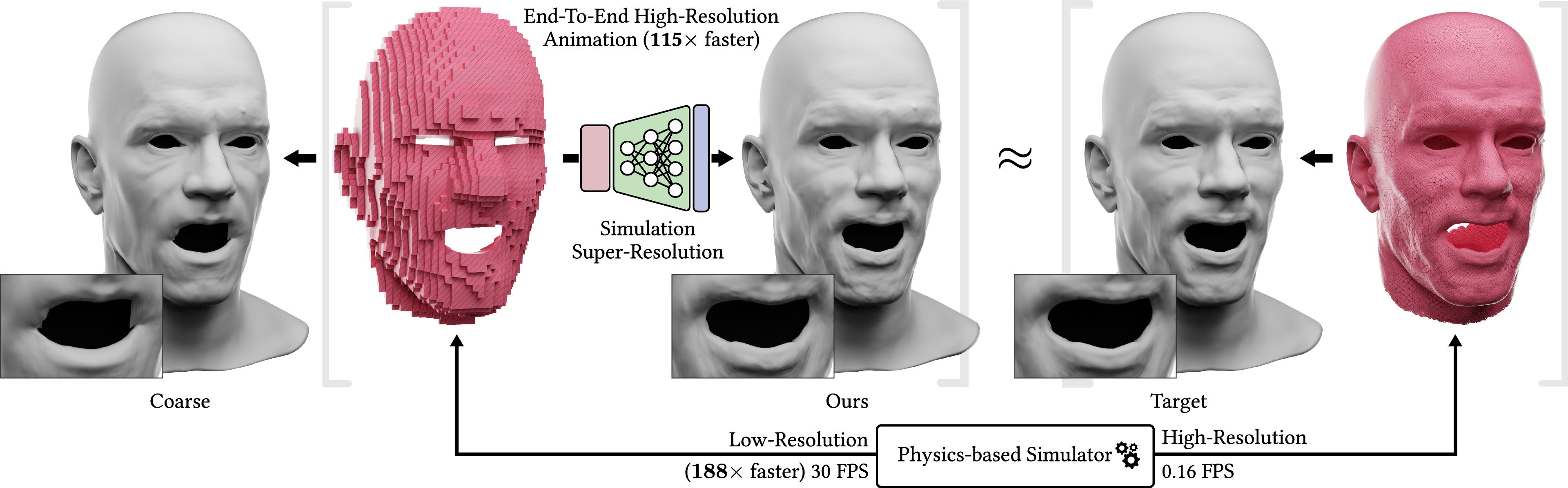
Figure 1. From left to right: Facial animation resulting from low-resolution simulation (Coarse), embedding low-resolution 3D mesh (red) simulating at 30.06 FPS, result of our simulation super-resolution framework (Ours), result from a corresponding off-line high-resolution simulation (Target), conforming high-resolution 3D mesh simulating at 0.16 FPS. Note the similarities between our result (Ours) and that from the high-resolution simulation (Target), which both differ from the result obtained by the low-resolution simulation (Coarse), especially around the mouth and chin area. Our simulation super-resolution achieves an effective 18.46 FPS, i.e. 115$\times$ faster than the high-resolution simulation. The low- and high-resolution meshes have 73 thousand and 1.9 million tetrahedra respectively, corresponding to a coarsening of $26\times$, and both simulations are accelerated with CUDA.

1. Introduction

Physics-based simulation is widely used to drive animations of both human bodies and faces. However, in order to obtain the highest levels of visual quality and realism, traditional simulation pipelines based on anatomic first principles resort to costly design choices. Detailed specifications of geometry and materials are essential, including the muscle and tendon shapes and attachment; bone geometry and motion; and constitutive properties of soft tissue and skin. Collision and frictional contact are ubiquitous in faces, and the resolution of such effects is dependent on mesh detail and the sophistication of detection and response algorithms. Finally, recreating intricate local shapes to match performance detail from real actors may impose further directability demands on the simulation pipeline. Such feature demands in conjunction with the sheer geometric mesh resolution necessary for detailed facial expressions often place reference-quality face simulation well beyond the cost that would allow for real-time performance.

This paper explores an alternative approach to achieving faithful and accurate facial animation at a much reduced execution cost, ideally as close as possible to real-time. Our method seeks to convincingly approximate a full, high-resolution 3D simulation with the combination of a simulator that uses lower resolution and model simplifications, paired with a deep neural network that boosts the resolution, detail, and accuracy of this coarse simulated deformation. Our simulation super-resolution module is trained on a dataset of coordinated performances crafted using the high- and low-resolution face simulators, and generalizes to novel performances by boosting the output of the low-resolution simulator to the quality anticipated from its high-resolution counterpart.

We aspire to create the best preconditions for the success of such a super-resolution module by focusing our attention on types of physics-based simulations where it may be possible to craft animations from the low- and high-resolution simulators that have strong semantic correspondence on a frame-by-frame basis. In other words, we look for types of simulation where it might be possible to infer – at some level of abstraction – what the fine-resolution simulation would want to do, by observing what the low-resolution simulator was able to do. Face simulation is a good exemplar of this concept; regardless of resolution, the same core drivers of deformation can be seen as being present in both cases: the action of muscles, and the kinematic state of skeletal bones and other collision objects. This allows us to create a training set by simply dialing in the same control parameters for these driving factors of simulations both in the low- and high-resolution models. Hence, we can hope that this semantic correspondence can be learned in a super-resolution neural network that generalizes this semantic correspondence between resolutions to unseen performances.

We highlight that even “semantically corresponding” simulated poses from the respective simulators described above can be quite different. In particular, the low-resolution result can deviate significantly from the mere downsampling of the high-resolution simulation, with discrepancies extending beyond high-frequency details. There are at least three core causes of such discrepancy: First, and most obvious, the reduced mesh resolution of the coarser simulation will be unable to resolve fine geometric features such as localized folds, wrinkles, and bulges that the fine-resolution mesh would capture. Second, the fact that governing physics and topology have to be represented using a coarser discretization may create bulk deviations from the expected behavior of the continuous medium. For example, the action of thin muscles might have to be dissipated over larger elements, reducing the crispness of their action. Fine topological features like the corners of the lips may be under-resolved, especially if at lower resolution we opt for an embedding simulation mesh that does not conform to the model boundary. Non-conforming embedded simulation offers well-conditioned elements and improved convergence that is attractive for real-time performance, but it also leads to a crude first-order approximation of the material volume for elements on the model boundary, leading to artificial stiffness and resistance to bending. The third and final contributor to bulk discrepancy between resolutions could be conscious design choices for the sake of interactive performance; for example, we may choose to perform elaborate contact/collision processing in our reference-quality simulation but forego collision processing altogether in the low-resolution simulator (as in our examples). Thus, our super-resolution module must account for much more than localized high-frequency deformation details and should compensate for all factors (mesh resolution, discretization non-convergence, physical simplifications) of bulk differences between the two simulation resolutions.

Our objective is to build a framework capable of producing high-accuracy animations without incurring the cost of simulations on high-resolution meshes. We achieve this by training a deep neural network to act as a super-resolution upsampler of simulations performed on a coarser 3D mesh. In practice, this allows for real-time simulations of facial animations that preserve many of the qualities associated with much slower high-resolution simulations.

We simulate a coarse low-resolution face mesh with significantly fewer mesh elements allowing for real-time simulations and reconstruct the high-resolution details learned from data. Our upsampling module accounts for both high-frequency details and bulk differences between resolutions, responses to dynamics and external forces, and can also approximate a degree of collision response even if collision handling is omitted from the low-resolution simulator. Our end-to-end animation attains near-realtime at 18.46 FPS from 30.06 FPS simulation and 47.82 FPS upsampling. We also emphasize that true real-time end-to-end animation (i.e., 24 or more FPS) is attainable by scaling down to coarser representations at a modest sacrifice of upsampling accuracy (discussed more in Sec. 5.4.1).

Previous efforts to accelerate physics-based simulations of deforming elastic bodies have focused on building faster numerical methods (Hauth and Etzmuss, 2001; Kharevych et al., 2006; Stern and Grinspun, 2009; Su et al., 2013), employing alternative constraint-based formulations such as Position Based Dynamics (Müller et al., 2007; Macklin et al., 2016; Bender et al., 2013) and its variants (Bouaziz et al., 2014; Liu et al., 2013; Stam, 2009), and other techniques such as adaptively computing higher resolutions only when needed (Bergou et al., 2007). However, given the real-time performance afforded by regular, embedded models for low-resolution simulations and the fast inferencing time of deep models, our framework can reconstruct high-resolution facial expressions faster and with reduced developmental effort.

We summarize our core contributions as follows:

$\bullet$ We extend the concept of super-resolution to the domain of physics-based simulation, contrasting with prior applications of this process to purely geometric 3D models, without regard to the fact the data originated from simulation.

$\bullet$ We demonstrate a neural network-based pipeline that can convincingly approximate a high-resolution facial simulation, using as input a real-time low-resolution approximate simulation and a fast inference step that performs the resolution boost. We show that this pipeline can robustly compensate for discrepancies between the two simulation resolutions extending beyond localized high-frequency deformation details.

$\bullet$ We identify the opportunity to create a training set for our super-resolution module with high degree of semantic correspondence between low- and high-resolution simulation frames, by giving the two simulators the same anatomical controls of muscle activations and bone kinematics.

$\bullet$ We demonstrate near-realtime performance of the end-to-end pipeline, and a robust ability to generalize to expressions not in the training set. We can even demonstrate this ability on deformations that extend beyond the parametric space used in the simulations that generated the training set (e.g. dynamics, external forces, collisions, or constraints not present in the training data).

2. Related Work

2.1. 3D super-resolution

Our framework shares the motivation (and also adopts the terminology) of super-resolution approaches that operate in the domain of images. Super-resolution (SR) was initially introduced for 2D images with the objective of restoring high-resolution images from their low-resolution observations (Nasrollahi and Moeslund, 2014). SR for 3D shapes shares similar characteristics with several relevant research areas.

Surface reconstruction

A closely related and widely studied area is a surface reconstruction from sampled points (Alexa et al., 2003). Prior research can be classified into two groups: global and local methods. Global methods are more robust than local methods against noise and sparsity of the observations but at the cost of reconstruction accuracy, and vice versa. Global methods include, namely, the RBF (Carr et al., 2001; Turk and O’brien, 2002; Ohtake et al., 2005b) and Poisson problem (Kazhdan et al., 2006; Kazhdan and Hoppe, 2013). On the other hand, local methods include MLS (Alexa et al., 2001, 2003; Fleishman et al., 2005), fitting of piecewise functions (Ohtake et al., 2005a; Nagai et al., 2009), and construction of signed distance functions (Curless and Levoy, 1996). A comprehensive review of this topic can be found in (Berger et al., 2017).

Point cloud upsampling

Another widely studied area that resembles several aspects of our work is point cloud upsampling, which has been actively explored by both traditional and learning-based methods for many applications such as robotics, autonomous cars and rendering (Zhang et al., 2022). A pioneering approach is PU-Net (Yu et al., 2018b) which operates on patches to learn per-point multi-level features and expands them through a multi-branch convolution network. Follow-up works include EC-Net (Yu et al., 2018a), 3PU (Yifan et al., 2019), PU-GAN (Li et al., 2019), PUGeo-Net (Qian et al., 2020), PU-GCN (Qian et al., 2021). While all the previous works supported only a fixed integer ratio of upsampling, Meta-PU (Ye et al., 2021) pioneered in adapting to arbitrary non-integer upsampling ratios.

Although we similarly adopt point cloud representations, we do not assume the input and output points are from the same geometry which motivates us to carefully design the upsampling method to adapt to the geometric discrepancy between the low- and high-resolution points and arbitrary non-integer upsampling ratios (Sec. 3.2 and more discussion in Sec. 5.4.2).

3D face super-resolution

Existing works focusing on 3D face SR can be categorized as either method- or learning-based methods. Method-based works include registration and filtering of the 3D acquisitions (Berretti et al., 2012, 2014; Bondi et al., 2016), whereas learning-based methods map from a low-resolution model to its high-resolution counterpart, namely, via intermediate cylindrical coordinate representations (Peng et al., 2005), progressive resolution chain (Pan et al., 2006), database retrieval (Liang et al., 2014), curve fitting (Zhang et al., 2020), and mapping from a set of rig parameters to the 2D deformation maps (Bailey et al., 2020). Recently, the problem was formulated as a point cloud upsampling to predict $z$-coordinates of the high-resolution face point cloud given its $(x,y)$ coordinates; however, the upsampling ratio is fixed by a factor of 2, and each $(x,y)$ coordinate can only correspond to a unique $z$ coordinate (Li et al., 2021).

In contrast to acquiring the low-resolution surface data from a 3D scanner, depth camera, or multi-view fusion, our work is rooted in a fast but fully volumetric physics-based simulator which allows us to provide as an input to our model a set of points that reach deep into the flesh volume and convey richer information about deformation and strain.

2.2. 3D Super-resolution in other domains

3D super-resolution has also been actively explored in different simulation domains, namely, garments and fluids. Notably, garment surface upsampling by learning of per-vertex deformations (Zurdo et al., 2012) and 2D normal map representations (Zhang et al., 2021) have been explored. For fluids, procedural (Kim et al., 2008) and GAN-based (Xie et al., 2018) methods have been explored to enhance the resolution of the simulated coarse turbulent flows.

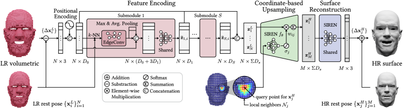
[r] Nvidia^©

Figure 2. The overview of our pipeline for 3D simulation super-resolution aiming at learning a mapping from a low-resolution (LR) volumetric mesh to a high-resolution (HR) surface mesh. Our pipeline is comprised of (1) Feature Encoding, (2) Coordinate-based Upsampling, and (3) Surface Reconstruction modules. The input and output are sets of 3D displacement vectors from the LR and HR rest pose shapes, respectively.

2.3. Coordinate-based MLPs

We employ coordinate-based multilayer perceptrons (MLPs) (Tancik et al., 2020) to model our upsampling (Sec. 3.2) and reconstruction modules (Sec. 3.3). Coordinate-based MLPs learn a continuous mapping from input coordinates to signals and have shown promising results for various visual tasks, such as image super-resolution (Chen et al., 2021), 3D shape representation (Mescheder et al., 2019; Park et al., 2019; Jiang et al., 2020; Saito et al., 2019), and novel view synthesis (Mildenhall et al., 2021; Ma et al., 2021; Chan et al., 2021). Recently, SIREN (Sitzmann et al., 2020) leverages periodic activation functions for implicit neural representations and has also demonstrated superior expressivity in modeling continuous and fine-detailed signals in various tasks (Chan et al., 2021; Ma et al., 2021; Yang et al., 2022).

3. Method

In this section, we present the specific design choices for our model architecture, aimed at learning to map from a low-resolution (LR) volumetric mesh to a high-resolution (HR) surface mesh depicting the same facial expression (Fig. 2). The input LR volumetric mesh contains 15,872 vertices and is derived from regular BCC (body-centered cubic) lattices for real-time simulation leveraging on its sparse and regular distribution of the vertices but with a compromise on accuracy and visual fidelity (Fig. 4c). On the other hand, the target HR mesh contains 35,637 vertices and is a triangular mesh conforming to a denser volumetric mesh capable of producing fine details of deformations but at a significantly slower simulation speed (Fig. 4b). More information about the data generation is outlined in Sec. 4.

We represent our input and output as point clouds, each structured as a set of 3D displacement vectors from a rest pose stacked in an arbitrary yet consistent order. We divide our pipeline into three modules for (1) feature encoding, (2) coordinate-based upsampling, and (3) surface reconstruction. The hyperparameters are specified in Appendix A.1.

3.1. Feature encoding network

The feature encoding network computes feature embedding for each input vector. We first concatenate each input displacement vector with a positional encoding $\in\mathbb{R}^{32}$ using sine and cosine functions as done in Transformers (Vaswani et al., 2017). Then, the concatenated input $\in\mathbb{R}^{D_{0}}$ (in our implementation, $D_{0}=35$) goes through the submodules of the feature encoding network.

While deformations in the human face are primarily attributed to the activation and motion of the underlying muscles and bones respectively, they can also be a result of deformations in other parts of the face (e.g., a wide smile can cause the skin around the eyes to fold); therefore, the localized per-vertex information of deformation needs to be shared with other vertices. For this reason, we model the submodules of the feature encoding network with edge convolutional layers, dubbed EdgeConv, introduced in DGCNN (Wang et al., 2019) which is capable of aggregating neighborhood information in feature space rather than coordinate space by dynamically constructing a $k$-NN graph in each layer.

We initialize the first $k$-NN graph of the network using geodesic distances based on the edge information of the LR mesh in the rest pose. The subsequent graphs are constructed on-the-fly in their learned feature spaces. The motivation is to encourage capturing local spatial correlations in the first submodule and potentially global feature correlations in the subsequent submodules (discussed more in Sec. 5.4.4).

We apply max and average pooling on the intermediate outputs from EdgeConv to extract global features. They are repeated and concatenated with the outputs from EdgeConv and the preceding input encoding feature, which are then passed through a shared fully connected network. We repeat the submodule $S=2$ times with the intermediate outputs from one module passed as input to the next. The output of the last submodule is concatenated with all of the previous $S$ intermediate features (including the position-encoded input) to construct the final encoded feature. Specifically, denoting the output of the $s^{th}$ submodule for the $i^{th}$ LR mesh vertex as $\mathbf{z}^{L}_{i}\in\mathbb{R}^{D_{s}}$, the final encoded output has the dimension of $\mathbf{z}^{L}_{i}\in\mathbb{R}^{\sum_{s=0}^{S}D_{s}}$. In our implementation, we used $S=2$ with $D_{1}=64$ and $D_{2}=128$.

3.2. Coordinate-based upsampling network

The upsampling network takes as the input a set of encoded per-vertex features from the LR mesh and outputs per-vertex features for the HR surface. To generalize over arbitrary and non-integer upsampling ratios, we propose to formulate the upsampling operation as a continuous local interpolation of the input features.

Formally, let the set of encoded features contributing to the upsampled $j^{th}$ feature be $\{\mathbf{z}^{L}_{i}\}_{i\in\mathcal{N}_{j}}$ where $\mathbf{z}^{L}_{i}$ denotes the encoded $i^{th}$ LR mesh feature, and $\mathcal{N}_{j}$ denotes a set of local interpolation neighbors for the $j^{th}$ feature. Then, the upsampling operation can be expressed as

(1) $$\mathbf{z}_{j}^{H}=\sum_{i\in\mathcal{N}_{j}}{w_{ij}\mathbf{z}^{L}_{i}}$$

, where $w_{ij}$ indicates the contribution of the $i^{th}$ LR mesh feature to the $j^{th}$ HR mesh feature. Different modeling options can be explored for defining the local neighbors set $\mathcal{N}_{j}$ (e.g., number and criteria of neighbors) and computing the interpolation weight $w_{ij}$ (e.g., inverse distance weighting (IDW), RBF, etc.), which we describe next.

Neighborhood locality

We define the local neighbors set $\mathcal{N}_{j}$ as the indices of the $k$ nearest LR mesh vertices from the $j^{th}$ HR mesh vertex in terms of geodesic distances (illustrated in the blue point cloud in center-bottom of Fig. 2). Since the LR and HR vertices do not live on the same surface, we first map the LR vertices $\{\mathbf{x}^{L}_{i}\}$ to the HR vertices (we temporarily denote the resulting mapped vertices as $\{\mathbf{x}^{\prime L}_{i}\}$) using the linear assignment algorithm (Crouse, 2016). This finds the optimal one-to-one mapping between the LR and HR vertices by minimizing the mapping distance (Euclidean). Then, we use Dijkstra’s algorithm to find the $k$ nearest mapped vertices $\{\mathbf{x}^{\prime L}_{i}\}$ (which directly corresponds to the original LR vertices $\{\mathbf{x}^{L}_{i}\}$) for every HR vertex using the edges of the HR surface mesh as paths (Fig. 3). The local neighbor information is pre-computed offline once. In this work, we use $k=20$ and additionally explore the effects of different values of $k$ in Sec. 5.4.

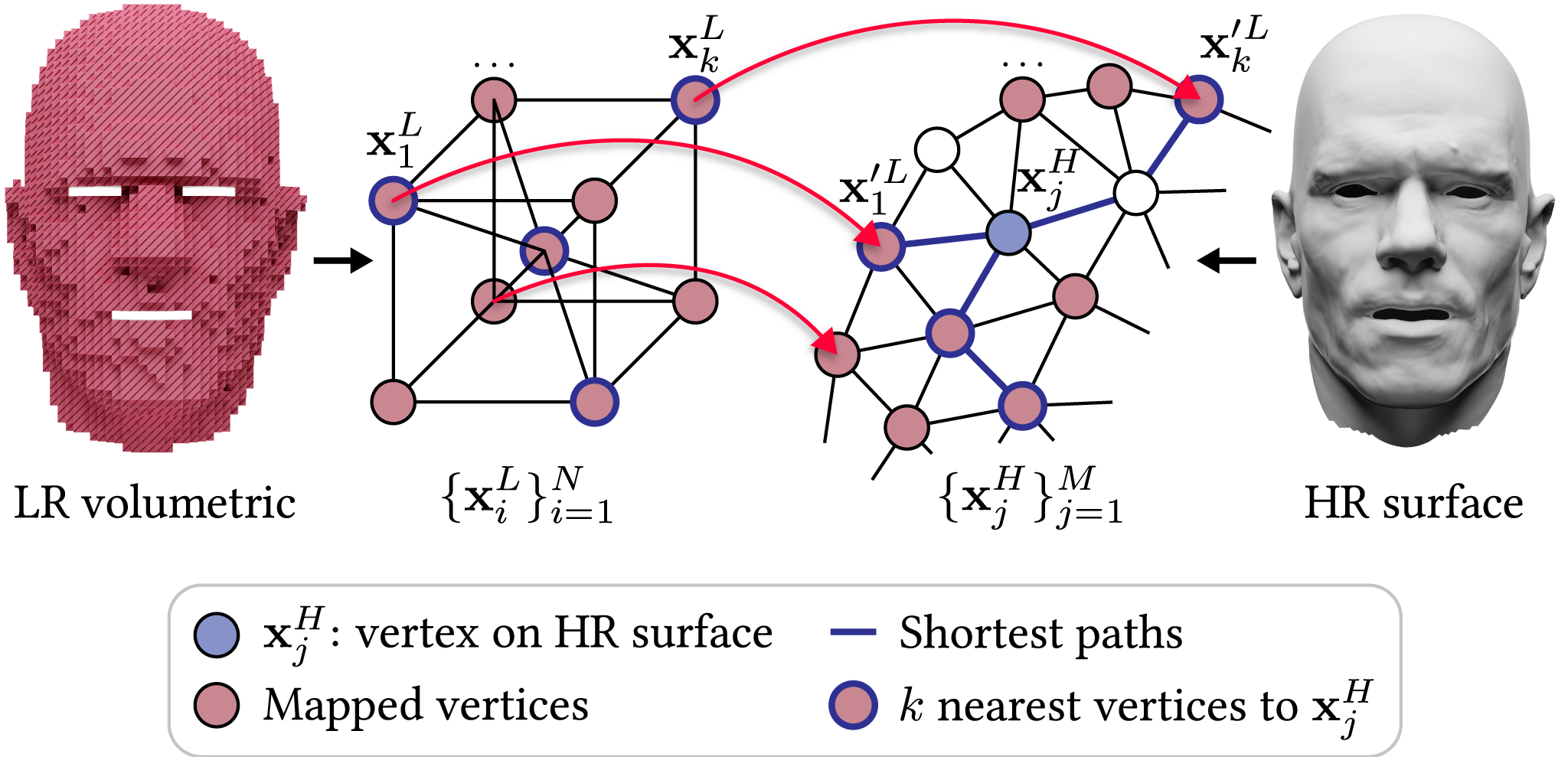
[r] Nvidia^©

Figure 3. Illustration of finding the $k$ nearest vertices $\{\mathbf{x}^{L}_{1},...,\mathbf{x}^{L}_{k}\}$ (where $i,...,k\in\mathcal{N}_{j}$) on the LR mesh to the vertex $\mathbf{x}^{H}_{j}$ on the HR mesh w.r.t. geodesic distances.

Weighting function

The weighting function $w^{\prime}_{ij}=f_{\theta}(\mathbf{u}_{ij})$ outputs the interpolation weight $w^{\prime}_{ij}\in\mathbb{R}$ for the $i^{th}$ LR mesh vertex neighboring the $j^{th}$ HR mesh vertex, given some input vector $\mathbf{u}_{ij}$.

Conceptually, the HR surface mesh can be thought of as a discretization of a continuous and smooth limit-surface, i.e. its vertices are approximations of the sampled points from the continuous surface. Thus, one could sample an infinite number of continuously varying features from any point on this surface. For this reason, we model $f_{\theta}$ as a trainable coordinate-based MLP where we employ SIREN (Sitzmann et al., 2020) for its superiority in modeling continuous (and differentiable) functions.

As the input to $f_{\theta}(\mathbf{u}_{ij})$, we provide the spatial information using a concatenated vector of coordinates of the HR and LR mesh vertices ($\mathbf{x}^{H}_{j},\mathbf{x}^{L}_{i}\in\mathbb{R}^{3}$, respectively) and their mutual Euclidean distance, written as

(2) $$\mathbf{u}_{ij}=[\mathbf{x}^{H}_{j},\mathbf{x}^{L}_{i},||\mathbf{x}^{L}_{i}-\mathbf{x}^{H}_{j}||_{2}].$$

Then, we normalize the output weight $w^{\prime}_{ij}$ across the local neighbors $\mathcal{N}_{j}$ using the softmax function $\sigma_{j}$ and obtain the final interpolation weight $w_{ij}$, expressed as

(3) $$w_{ij}=\sigma_{j}(w^{\prime}_{ij}|\{w^{\prime}_{kj}\}_{k\in\mathcal{N}_{j}})=\frac{e^{w^{\prime}_{ij}}}{\sum_{k\in\mathcal{N}_{j}}e^{w^{\prime}_{kj}}},$$

for $j=1,...,M$ and $i\in\mathcal{N}_{j}$.

3.3. Surface reconstruction network

The surface reconstruction network predicts the per-vertex displacements $\Delta\mathbf{x}_{j}^{H}$ from the upsampled features $\mathbf{z}_{j}^{H}$. Since $\mathbf{z}_{j}^{H}$ implicitly inherits coordinate information $\mathbf{x}_{j}^{H}$ from the upsampling network and to reconstruct fine deformation details on the HR surface, we also model the surface reconstruction network using SIREN (Sitzmann et al., 2020) to exploit its ability to model high-frequency signals utilizing coordinate information. As the last step, the predicted deformations are added to the HR mesh in its rest pose to reconstruct the final deformed HR surface.

We also note that we use a minimal modeling technique for the surface reconstruction network not only to reduce the computational overhead for processing a relatively large number of HR mesh vertices ($>~{}36k$), but also because we assume all the information needed for the fine-detailed surface reconstruction is to be encoded in the LR mesh features.

3.4. Loss function

We minimize the reconstruction loss $\mathcal{L}_{recon}$ between the predicted and ground-truth per-vertex deformations of the HR surface mesh denoted $\Delta\hat{\mathbf{x}}_{j}^{H}$ and $\Delta\mathbf{x}_{j}^{H}$, respectively:

(4) $$\mathcal{L}_{recon}=\sum_{j=1}^{M}||\Delta\hat{\mathbf{x}}_{j}^{H}-\Delta{\mathbf{x}}_{j}^{H}||_{1}.$$

Moreover, we introduce the loss term $\mathcal{L}_{fn}$ for local smoothness which encourages the face normal of triangles on the predicted and target HR surface meshes (denoted $\hat{\mathbf{n}}_{k}$ and $\mathbf{n}_{k}$, respectively) to be equivalent in terms of cosine similarity:

(5) $$\mathcal{L}_{fn}=\sum_{k=1}^{F}1-\frac{\hat{\mathbf{n}}_{k}\cdot\mathbf{n}_{k}}{||\hat{\mathbf{n}}_{k}||||\mathbf{n}_{k}||},$$

where $F$ is the number of triangles on the HR surface mesh.

We also include the regularization term $\mathcal{L}_{reg}$ to encourage the encoded intermediate features $\{\{\bar{\mathbf{z}}_{s,i}\}_{i=1}^{N}\}_{s=1}^{S}$ (Fig. 2) to center around 0, encouraging their prior to follow a multivariate normal distribution (Park et al., 2019; Chabra et al., 2020):

(6) $$\mathcal{L}_{reg}=\sum_{s=1}^{S}\sum_{i=1}^{N}||\bar{\mathbf{z}}_{s,i}||_{F}.$$

We find that the face normal loss improves the visual fidelity of the reconstructed face and the regularization term helps prevent overfitting.

The final loss function $\mathcal{L}$ is written as

(7) $$\mathcal{L}=\mathcal{L}_{recon}+\alpha\mathcal{L}_{fn}+\beta\mathcal{L}_{reg},$$

where $\alpha$ and $\beta$ are the scalar weight terms whose values are reported in Table 3 of the Appendix.

4. Dataset Generation

In this section, we outline the process for acquiring the mesh models and attachment of muscle fibers, as well as our simulation framework for synthesizing the dataset consisting of the low-resolution (LR) volumetric simulation mesh for flesh and the corresponding high-resolution (HR) surface mesh for the face as shown in Fig. 4.

4.1. Acquisition of simulation models

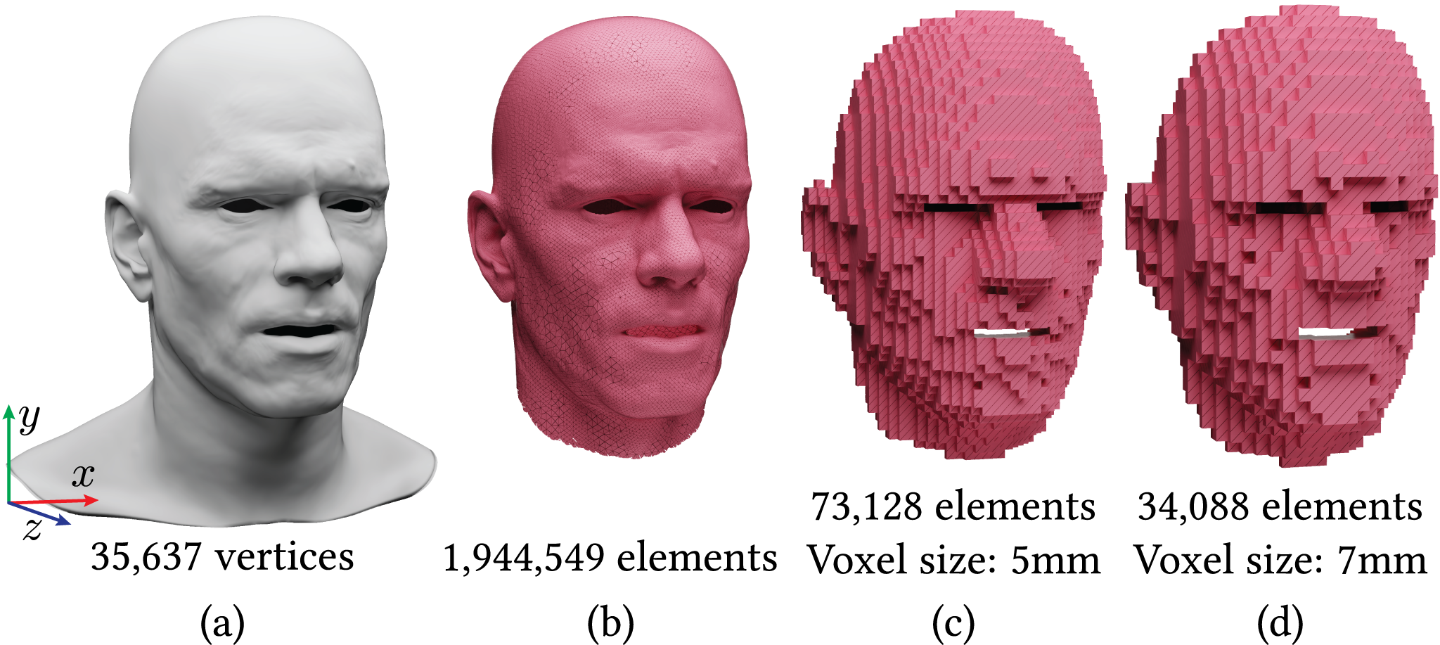
[r] Nvidia^©

Figure 4. (a) High-resolution surface model in dimensions of $289.0\times 342.7\times 291.1$ [mm] w.r.t. $x$, $y$, and $z$ axis, respectively, including the part of the shoulder, (b) high-resolution simulation model (0.16 FPS simulation), (c) low-resolution simulation model (30.06 FPS simulation) for the near-realtime end-to-end animation at 18.46 FPS, and (d) coarser low-resolution simulation model (67.79 FPS simulation) for the true real-time end-to-end animation at 28.04 FPS.

In this section, we explain the process for sculpturing our low-resolution (LR) and high-resolution (HR) simulation models ((b) and (c) in Fig. 4, respectively) which are then used for generating semantically corresponding facial animation dataset.

Anatomical model

Following prior common approaches (Sifakis et al., 2005; Cong et al., 2015), we construct an anatomically and biomechanically motivated simulation model of our subject’s face. Given a HR neutral face mesh, we model the underlying anatomy including the cranium, mandible, teeth, and a comprehensive set of facial muscles with the aid of anatomical references. For each facial muscle, we calculate volumetric fiber directions by first tetrahedralizing the muscle and then applying the approach of (Choi and Blemker, 2013). Alternatively, a morphing approach such as (Ali-Hamadi et al., 2013; Cong et al., 2015) can also be employed to estimate the underlying anatomy.

High-resolution volumetric mesh

For our highest resolution model, we create a tetrahedral simulation mesh consisting of 1.9 million tetrahedra (Molino et al., 2003) (Fig. 4b) that conforms to the HR neutral face mesh (Fig. 4a) as well as the underlying skull. We opted for a conforming tetrahedralized simulation mesh in order to maximize deformation accuracy and minimize artificial stiffness often associated with non-conforming tetrahedra. The tradeoff is the potential for less well-conditioned tetrahedra and longer simulation times. Before generating our HR dataset, we validated our high-resolution anatomical model against high-resolution facial performance capture data including a set of 33 artist-sculpted blendshapes for a variety of facial expressions. Then, we extended our simulation framework to also be differentiable following the approach outlined in (Bao et al., 2019) by constructing a blendshape muscle rig from these blendshapes and using the corresponding blendshape weights to parameterize our simulation.

Low-resolution volumetric mesh

For our LR model, we create a regular nonconforming tetrahedralized simulation mesh consisting of 73 thousand tetrahedra (Fig. 4c), to be used in an embedded simulation. We begin by voxelizing the HR conforming tetrahedron mesh at a coarse granularity and discarding tetrahedra outside the regions of the face most responsible for facial expression, including the neck and the back of the head. Then, we subdivide each voxel into eight regular tetrahedra. In constrast to our HR model, our nonconforming regular LR model consists of regular well-conditioned tetrahedra that enables us to target real-time simulation. In order to avoid merging the upper and lower lips with our coarse discretization, we separate the lips via linear blend skinning, pre-deforming the high-resolution conforming tetrahedralized simulation mesh by a small rotation of the jaw joint along its axis. This results in a rest configuration with the mouth slightly open; this necessary modeling discrepancy is among the factors that our super-resolution network must compensate for (and is largely successful in doing so).

Muscle fibers and attachments

For both the high- and low-resolution simulation meshes, we then follow in the steps of prior anatomic simulation work (Sifakis et al., 2005; Cong et al., 2016) and rasterize the volumetric muscle fiber directions while also computing kinematic muscle tracks. Then, we specify cranium and jaw attachments of the muscles on both simulation meshes via Dirichlet boundary conditions. Finally, the high-resolution neutral face mesh (containing 61,520 vertices) is embedded in both the high and low-resolution simulation mesh respectively via barycentric weights enabling us to deform the face mesh by interpolating vertex positions from the respective deformed simulation mesh.

Discrepencies between high- and low-resolution surfaces

Fig. 5 illustrates the discrepancies between the surface embedded in the simulated LR mesh and the surface simulated using the conforming HR mesh. Even though the two performances show semantic similarities, there have both macroscopic (lips) and microscopic (forehead and eyes) differences owing to simulation resolution.

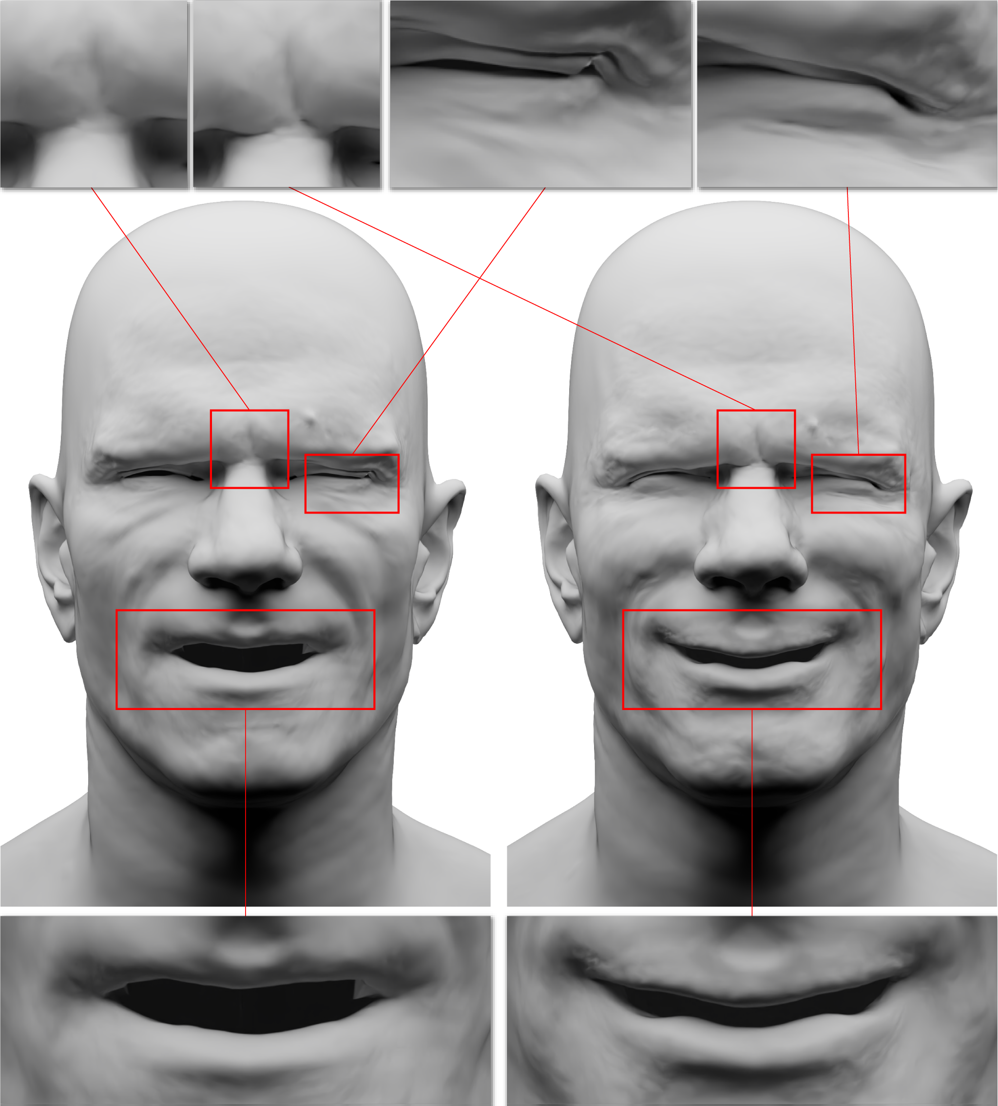
[r] Nvidia^©

Figure 5. The face surface embedded in the non-conforming low-resolution volumetric mesh with 73k tetrahedra (left) deviates significantly from the same surface simulated using a conforming high-resolution mesh with 1.9m tetrahedra (right), even though both deformations are parameterized using the same blendshape weights and jaw transformation. We zoom into different regions of the face to highlight macro and microscopic discrepancies.

4.2. Simulation framework

We employ a CUDA-accelerated implementation of (Cong et al., 2016) as our simulation framework for both resolutions. This framework endows the simulation mesh with the anisotropic constitutive model consisting of three components for modeling elasticity, incompressibility, and muscle contractions (Teran et al., 2003) as well as zero-length track springs for additional expressivity and directability. Both the finite element forces and the track spring stiffness are parameterized to be invariant to mesh refinement in order to maintain consistent bulk behavior across resolutions. Given a set of control parameters, we calculate the deformation of the tetrahedralized simulation mesh using the quasistatic framework of (Teran et al., 2005), factoring in object and self-collisions for the high-resolution simulation. In contrast, we forgo collision handling in our LR simulation for the sake of robustness and performance.

High-Resolution Dataset

Using the Gauss-Newton optimization framework proposed in (Sifakis et al., 2005), we targeted four sequences of high-fidelity facial performance capture data corresponding to four different semantic themes (amazement, anger, fear, and pain) totaling 880 frames using our HR simulation mesh. This results in a simulated HR simulation and surface mesh, as well as time-varying blendshape weights and jaw transforms for each performance.

Low-Resolution Dataset

Since our facial muscles are in correspondence between the HR and LR, we can use the same blendshape muscle rig to drive the LR simulation and synthesize a corresponding LR dataset. We use the blendshape weights and jaw transforms resulting from the HR optimization as input into our LR simulation and run the quasistatic solver to obtain the corresponding LR tetrahedral simulation mesh deformations across all four sequences. The discrepancies between the surfaces embedded in the simulated LR mesh and conforming HR mesh, respectively, are illustrated in Fig 5 of Sec. 4.1.

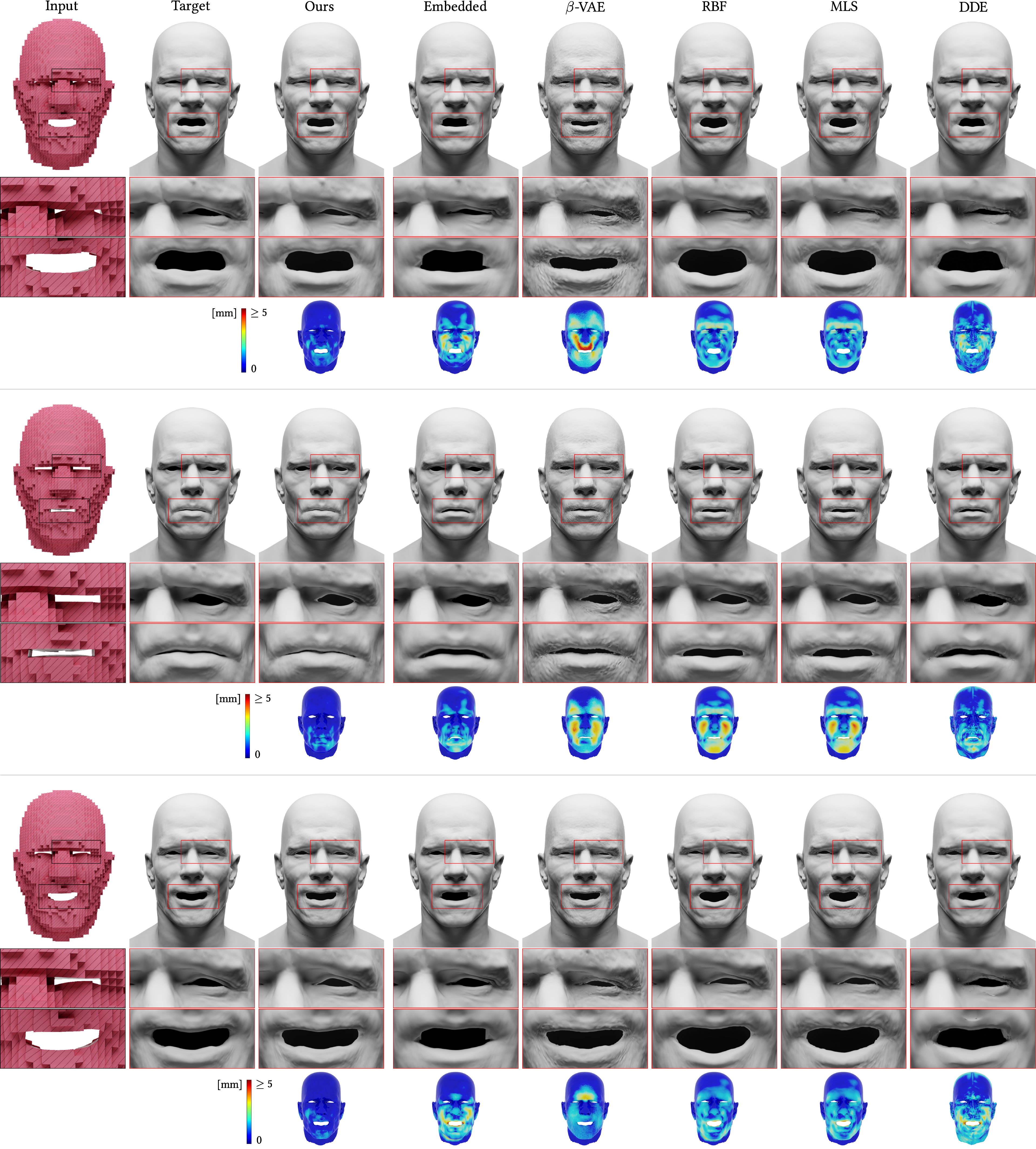
[r] Nvidia^©

Figure 6. Our method can generalize to unseen facial expressions and reconstruct the target face with high accuracy compared to the standard embedded surface and other tested models ($\beta$-VAE, RBF, MLS, and DDE). The second and third rows show the left eye and mouth zoomed-in, respectively. The heatmaps visualizing the reconstruction errors are shown in the respective last rows.

5. Experiments and Evaluation

We report performance metrics in terms of reconstruction speed (Sec. 5.1) and as well as quantitative and qualitative reconstruction errors (Sec. 5.2). We use the unseen performances in the test set to evaluate the generalization capacity of the trained model. We also evaluate our framework’s ability to generalize to unseen dynamics and forces (Sec. 5.3).

We also conduct ablation experiments. In Sec. 5.4.1, we explore the trade-offs in the reconstruction performance of our model when trained using the coarser low-resolution volumetric mesh capable of attaining the true real-time end-to-end animation at 28.04 FPS as compared to our recommended near real-time at 18.46 FPS. In Sec. 5.4.2, we explore how the submodules of our framework, namely Feature Encoding and Coordinate-based Upsampling modules, contribute to the reconstruction accuracy and, in Sec. 5.4.3, evaluate the effects of using different interpolation neighbors $\mathcal{N}_{j}$ for the Coordinate-based Upsampling network and different neighbors $k$ for the $k$-NN graph from the Feature Encoding network. Then in Sec. 5.4.4, we qualitatively evaluate the correlations among different parts of the face learned by the EdgeConv layers in the Feature Encoding submodules. Additionally in Sec. A.2.5, we explore our framework’s ability to approximate self-collisions between the upper and lower lips.

5.1. Near-realtime high-resolution facial animations

Simulations speed

The average time to simulate the high-resolution conforming simulation with 1,944,549 tetrahedral elements is 6.22s per frame or a frame rate of 0.16 FPS. Conversely, the average time to simulate the low-resolution embedding mesh with 73,128 tetrahedral elements is 0.033s, corresponding to 30.06 FPS, i.e. 188$\times$ faster than the high-resolution simulation. These simulation times are recorded on a workstation with a single GeForce RTX 4090 GPU.

Super-resolution inference speed

To approximate the high-resolution surface from the low-resolution simulation, we need to infer the high-resolution displacements from our model. The computational overhead of our model inference on a single GeForce RTX 4090 GPU is 0.0209s per frame, corresponding to 47.82 FPS for inference alone.

End-to-end speed and additional performance boosting

Consequently, our simulation super-resolution framework takes a total of 0.054 FPS per frame, or 18.46 FPS, which implies that we achieve a speedup of 115$\times$ relative to the high-resolution simulation that takes 6.22s per frame (0.16 FPS). We emphasize that there are multiple ways to bridge the gap from near-realtime, e.g. 18.46 FPS, to true real-time, i.e. $24$ or more FPS.

First and foremost, using a coarser low-resolution simulation mesh can easily attain the true real-time end-to-end animation given tolerance to a minute trade-off in the quality of reconstructions which our current low-resolution mesh enjoy (we explore the trade-off in Sec. 5.4.1). Similarly, we can also achieve faster inference time by choosing to use fewer interpolation neighbors in the Coordinate-based Upsampling module but with a trade-off in the overall reconstruction accuracy (see Sec. 5.4), as we identify the bottleneck of inference is the neighborhood information gathering step in the Coordinate-based Upsampling module.

On the other hand, while adhering to the strict bar for the permissible reconstruction quality, we could pipeline the low-resolution simulation and inference steps using a 2 GPU workstation. In such a set up, we could achieve an end-to-end speed of 30.06 FPS after tolerating a single frame latency. Conversely, we could also move away from the inference library (we use ONNX Runtime for PyTorch) and implement custom inference kernels on GPUs that speed up computation.

5.2. Generalization to unseen facial expressions

Using the simulation data, generated as described in Sec. 4, we select the amazement and pain sequences for training (435 frames) and test on anger and fear sequences (445 frames), ensuring that the test set contains unseen performances. We use the trained model to infer the high-resolution face surface from unseen low-resolution volumetric mesh performances in the test set.

Quantitative evaluation

As we have access to the high-resolution simulations of the test data, we can readily compute the reconstruction error in terms of per-point Euclidean distance between the reconstructed and the target (reference) mesh whose dimension is $179.8\times 257.3\times 164.5$ [mm] (Fig. 4). We also set up other commonly used reconstruction methods to serve as comparisons for our method. We train a $\beta$-VAE (Higgins et al., 2016), on the same data set to serve as a baseline generative neural framework comparison. We implement two of the commonly used surface reconstruction methods: the radial basis function (RBF) and moving least-square (MLS)-based methods as the representative global and local methods, respectively. Lastly, we compare with Deep Detail Enhancement (DDE) framework (Zhang et al., 2021) as the representative state-of-the-art super-resolution framework for 3D garment surfaces which uses normal maps to synthesize plausible wrinkle details on a coarse geometry. The formulations for RBF and MLS along with details on the $\beta$-VAE and DDE can be found in Sec. A.2.1, A.2.2, A.2.3, and A.2.4, respectively.

Our method outperformed the others and robustly achieved the lowest mean reconstruction errors per frame $<$0.59mm. We plot the frame-wise mean reconstruction errors of the comparisons to validate that our method has the least error for every test performance in Fig. 7. The evaluation result is summarized in Table 1.

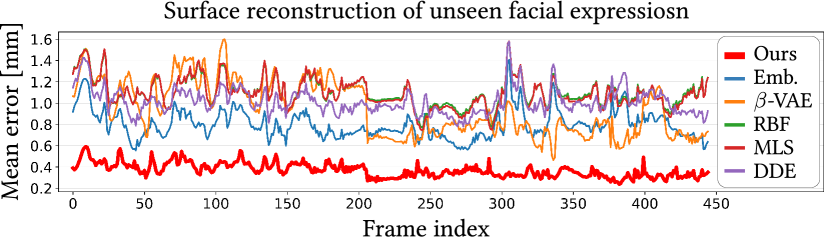
Figure 7. Frame-wise mean surface reconstruction error of unseen facial expressions for each tested model. Our method (in red line) achieved the lowest mean error across every test frame.

Table 1. Descriptive statistic measures (normalized mean, median, standard deviation, and min/max values for each method) of mean surface reconstruction errors (in millimeters) on unseen facial expressions for each tested model.

[mm]	Mean	Median	Std.	Max.	Min.
Ours	0.37	0.36	0.07	0.59	0.24
Embedded	0.80	0.77	0.13	1.40	0.55
$\beta$-VAE	0.94	0.87	0.25	1.60	0.46
RBF	1.10	1.08	0.13	1.57	0.77
MLS	1.09	1.07	0.14	1.58	0.74
DDE	1.01	0.99	0.12	1.58	0.78

Qualitative evaluation

In Fig. 6, we evaluate the visual fidelity of the inferred face mesh by visualizing the reconstructed high-resolution surfaces and heatmaps of corresponding reconstruction errors for all the methods. Our method can infer the target facial expression from the input low-resolution volumetric mesh more faithfully than other methods, allowing us to conserve both the expression and the subtle deformation details that otherwise would have been compromised by using the low-resolution simulation.

5.3. Generalization beyond parametric space

We test the ability of our framework to handle deformations that extend beyond the parametric space used in simulations. To evaluate, we simulate the low-resolution simulation mesh with unseen dynamics and external forces, respectively, and qualitatively evaluate the inference accuracy.

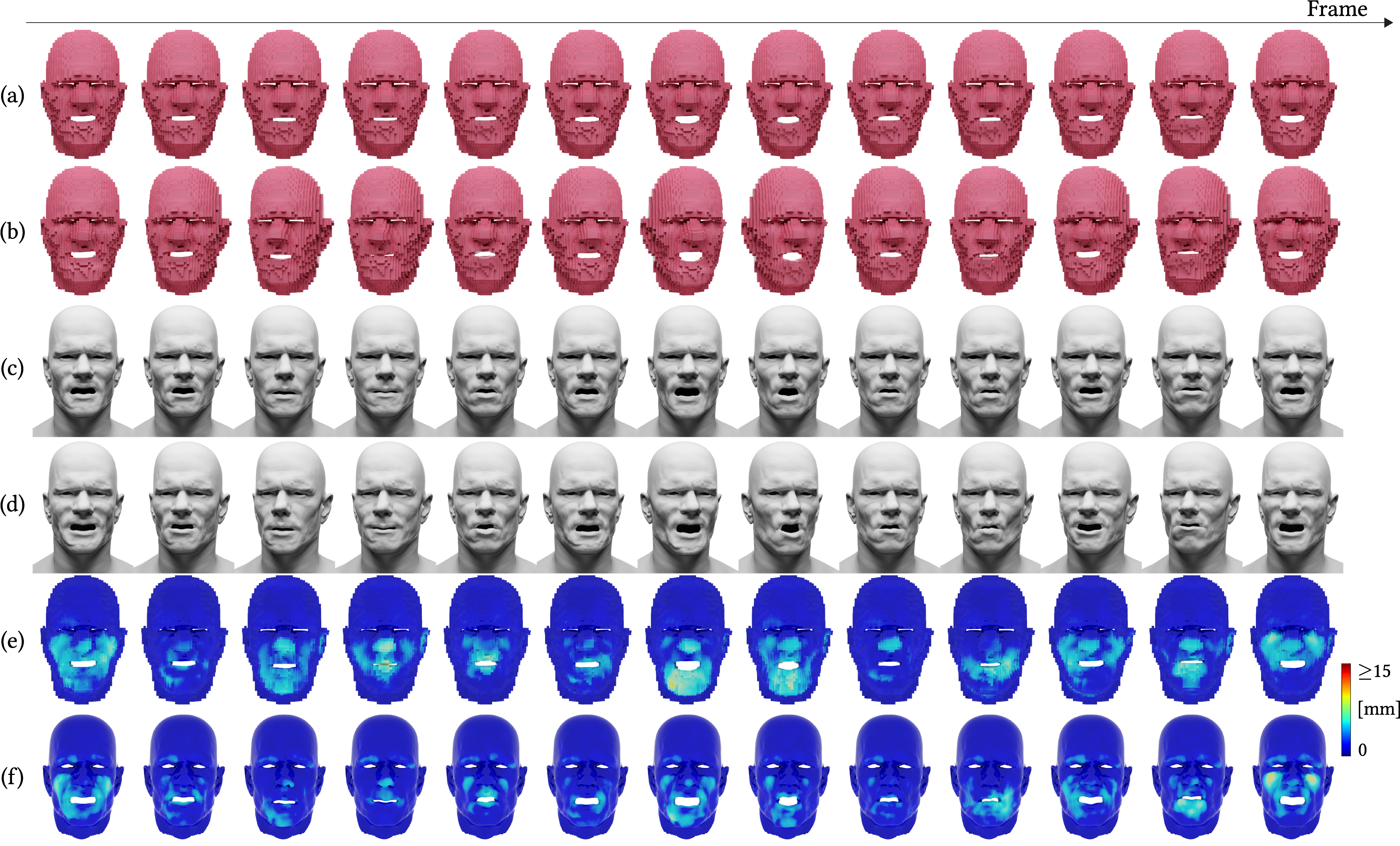
[r] Nvidia^©

Figure 8. Visualization of sequential frames. From top to bottom: The low-resolution input meshes simulated using (a) a quasi-static and (b) dynamic scheme with left-and-right head spin motions. (c) The high-resolution target faces conforming to the high-resolution quasi-static simulation mesh. (d) Reconstructed surfaces inferred from (b). (e)/(f) The heatmaps showing deformation differences between the meshes $\{$(a), (b)$\}$ and $\{$(c), (d)$\}$, respectively.

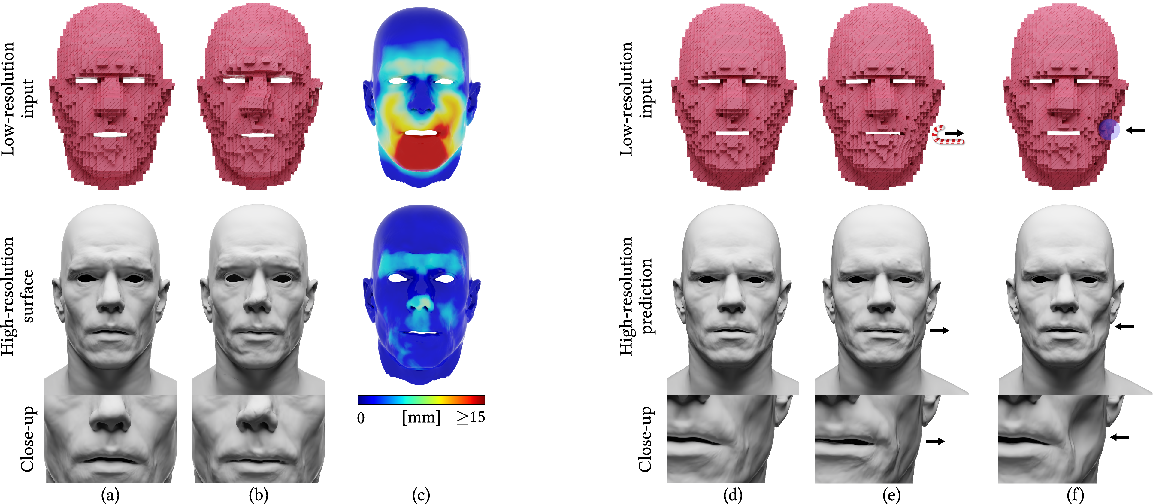
[r] Nvidia^©

Figure 9. We test the ability of our framework to handle deformations that extend beyond the parametric space used in the simulation by visualizing the inferred surfaces from unseen dynamics (left) and external forces (right) (Sec. 5.3).

5.3.1. Unseen dynamics

To evaluate our model’s capability in generalizing to non-quasi-static simulations, we simulate the dynamics of the low-resolution simulation mesh using a semi-implicit backward Euler scheme. This allows us to model ballistic effects that are not present in our training dataset which was simulated under the quasi-static assumption. We further exaggerate the ballistic effects in the simulation by shaking the head back and forth in conjunction with the muscle contractions and jaw motion.

We compare the reconstructed surface inferred from the input mesh with unseen dynamics (middle row of Fig. 9b) and the reference surface conforming to the quasi-static simulation mesh (middle row of Fig. 9a). Also, we visualize heatmaps showing average facial deformations across the training data (top row of Fig. 9c) and the deformation differences between the predicted and reference surfaces, respectively (middle row of Fig. 9c). We highlight that although the nose shows little or no deformations throughout the training data (thus, showing the nose as a dark blue region in the first heatmap), our model is capable of inferring them from the unseen input (showing as a lighter blue region in the second heatmap).

Similarly, we visualize the dynamic simulations and reconstructions in a time sequence in Fig. 8 along with the heatmaps (Fig. 9e-f) showing deformation differences between the quasi-static and dynamic simulation meshes (Fig. 9a-b) and also the reference conforming quasi-static surface (Fig. 9c) and the reconstructed surface inferred from the dynamic low-resolution simulation mesh (Fig. 9d), respectively. Regions with distinctive facial deformations of the inferred faces (Fig. 8e) are in line with the deformed regions of the input simulation meshes (Fig. 8f), implying generalizations beyond the quasi-static simulation data.

5.3.2. Unseen forces

We craft two quasi-static simulation examples with external forces applied. In the first example (left of Fig. 9e, apply a spring force pulling the side of the lips. This force can also be interpreted as a candy cane pulling on one side of the lips. In the second example (Fig. 9f), we collide the low-resolution embedding mesh with a sphere, pushing the cheek inward. The low-resolution performances, reconciled by the simulator, are given as input to our framework. The predictions (shown in Fig. 9) indicate that our framework is able to handle inputs that have deformations not seen in the training performances.

5.4. Ablation experiments

In this section, we compare the quality of reconstructed faces inferred by our model trained using the original low-resolution simulation mesh with 73k elements (Fig. 4c) and another one trained using a coarser low-resolution simulation mesh with 34k elements (Fig. 4d). The coarser mesh attains the true real-time end-to-end animation at 28.04 FPS (67.79 FPS simulation and 47.82 FPS inference) on the same hardware setup.

Furthermore, we evaluate the contributions of our Feature Encoding (Sec. 3.1) and Coordinate-based Upsampling (Sec. 3.2) modules. We explore the effects of the key parameters in each of the two modules, namely, the neighbors $k$ in the feature encoding module and the interpolations neighbors in the upsampling module, respectively. Additionally, we qualitatively validate the correlations among different parts of the face learned by our feature encoding network.

5.4.1. Comparison with coarser low-resolution simulation mesh

For training, we use the same hyperparameters as the training on the original low-resolution simulation mesh. Following the same procedure in Sec. 5.2, we evaluate the surface reconstruction errors on the unseen facial expressions in the test dataset.

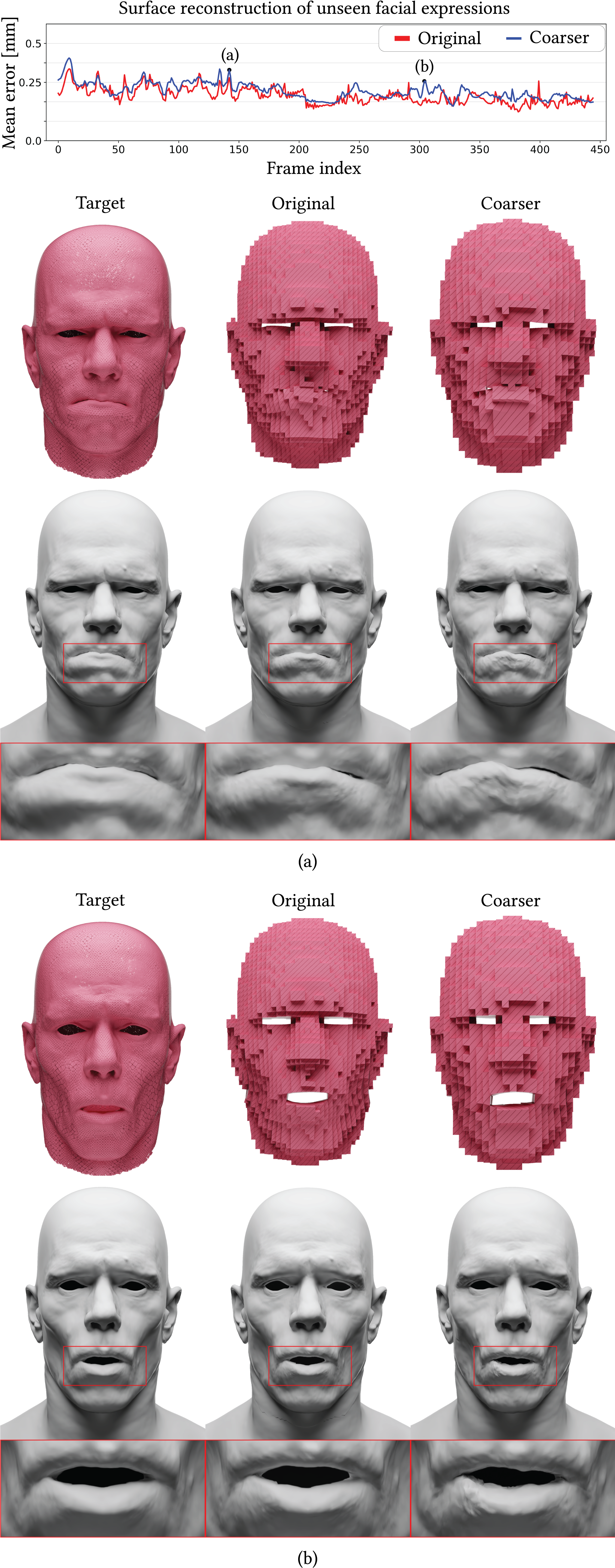
[r] Nvidia^©

Figure 10. Comparisons of the surface reconstruction qualities by our model trained using the original low-resolution simulation mesh (73k elements) and a coarser mesh with half the resolution (34k elements), respectively. We visualize the reconstructed surfaces in (a) and (b).

As shown in the error plot of Fig. 10, using the coarser low-resolution mesh expectedly attains slightly larger reconstruction errors across most of the frames compared to the original mesh. We observe increased artifacts in the inferred surfaces especially around the mouth regions in Fig. 10a-b. We highlight that, in practice, true real-time end-to-end animation is easily attainable had we tolerated a minute deterioration of the reconstruction quality which could become unnoticeable to human eyes with different rendering techniques such as using texture map as opposed to a plain diffuse rendering. However, we choose to adhere to the current resolution for the robustness of generalization capabilities beyond the parametric space used in the simulation (e.g., unseen dynamics and external forces), given that true real-time animation is also attainable, in practice, had we tolerated one frame latency.

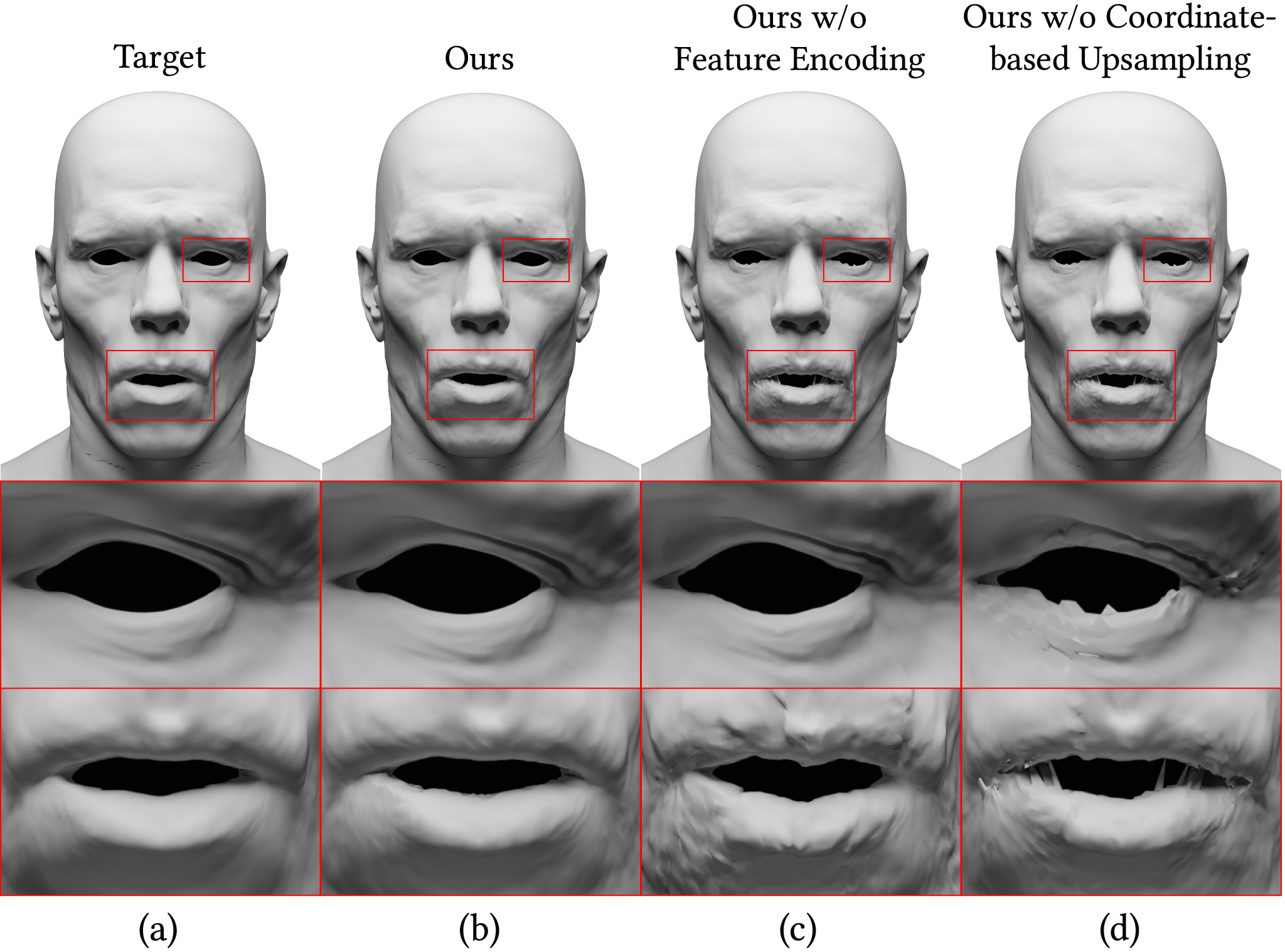
[r] Nvidia^©

Figure 11. We visualize predictions on a test performance from 3 models - our proposed framework (b), model with feature encoding module excluded (c) and model with the coordinate-based upsampling module replaced (d). The same test performance, simulated in high resolution is visualized in (a).

5.4.2. Contributions of Feature Encoding and Coordinate-based Upsampling modules

We evaluate the contributions of the Feature Encoding (FE) and Coordinate-based Upsampling (CU) modules by excluding them (one at a time). We compare the predictions on test performances.

Specifically, we train 3 different models using the same dataset and hyperparameters for the same number of epochs (1000). The first model we train includes both the FE and CU modules (our proposed framework). The second model excludes the FE module and directly feeds the output of position-encoding to the CU module. In the third model, we reintroduce the FE module and exclude the CU module. To replace the CU module, we opt for a different and standard upsampling method (with a fixed upsampling ratio) that uses the transposed convolution operation, widely adopted in upsampling images for super-resolution (Yang et al., 2019). To mimic the transposed convolution operator, we find 20 nearest LR mesh vertices from each HR mesh vertex in terms of Euclidean distance (same number as our neighbor interpolation in the CU module). We then compute weighted sums of the 20 LR mesh features for every HR mesh vertices. For a fair comparison, we learn these weights, similar to the weights learned in our CU module.

From the 3 trained models, we compare the reconstruction error on the test dataset. As summarized in Table 2, our model which includes both the Feature Encoding and Coordinate-based Upsampling modules outperforms the other two variants which have been trained in the absence of the Feature Encoding and Coordinate-based Upsampling modules, respectively.

Table 2. Descriptive statistic measures of surface reconstruction errors in the absence of our Feature Encoding (FE) and Coordinate-based Upsampling (CU) network.

[mm]	Ours	w/o FE	w/o CU
Mean	0.38	0.45	0.59
Std.	0.06	0.07	0.10
Median	0.38	0.45	0.58
Max.	0.64	0.75	1.11
Min.	0.27	0.33	0.41

We qualitatively validate the visual fidelity of the performances reconstructed by the three models in Fig. 11. We observe that in the absence of the FE module, the model fails to reconstruct the parts of the face with larger deformations accurately (like the mouth area in Fig. 11c), and replacing the CU module leads to reconstruction artifacts and discontinuities in the high-resolution surface (Fig. 11d).

5.4.3. Effects of different locality parameters

Interpolation neighbors in Coordinate-based Upsampling

We explore the effects of using a different number of interpolation neighbors for defining the local neighbors set $\mathcal{N}_{j}$ in Sec. 3.2. For this experiment, we train our model using the same training dataset and hyperparameters for 500 epochs but vary the number of interpolation neighbors as 1, 3, 5, 10, and 20. We fix $k=5$ for the $k$-NN graph in the Feature Encoding module for these experiments. We plot the mean surface reconstruction error on the test dataset to study the effect of varying the number of interpolation neighbors on reconstruction accuracy.

As shown in the plot in Fig. 12a, we observe that using a higher number of interpolation neighbors achieves lower mean reconstruction error on unseen performances (shown in red). However, the trade-off is a linearly increasing time consumption for each inference (shown in blue).

Number of neighbors $k$ in Feature Encoding

We conduct another experiment to study the effect of varying the neighbors $k$ used in constructing the $k$-NN graph in the EdgeConv layer of the Feature Encoding module. We train our model for 500 epochs while varying $k$ from 1 to 10 in each experiment, and evaluate the mean surface reconstruction error on the test dataset. We fix the number of interpolation neighbors in the Coordinate-based Upsampling module to 10 for these experiments. As shown in the plot in Fig. 12b, we find that using $k=4,5$ gives the minimum reconstruction error (shown in red) without a large trade-off in the inference time (shown in blue).

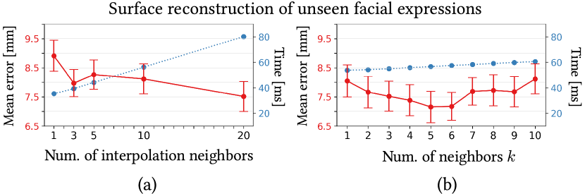
Figure 12. Surface reconstruction errors on unseen facial expressions (red plots) as a function of the number of interpolation neighbors (left) and the number of neighbors $k$ for the $k$-NN graphs in Feature Encoding submodules (right). The blue plots show the inference time per frame for each of the tested values.

5.4.4. Correlations learned in Feature Encoding module

We visualize the heatmaps of the feature similarities learned by the EdgeConv layer in the second Feature Encoding network submodule. This can reveal the correlations among different parts of the face learned from data. As outlined in Sec. 3.1, we encourage the first submodule to learn local spatial correlations by constructing the $k$-NN graph in based on geodesic distances, and the second submodule to learn (potentially global) feature correlations in its learned feature space.

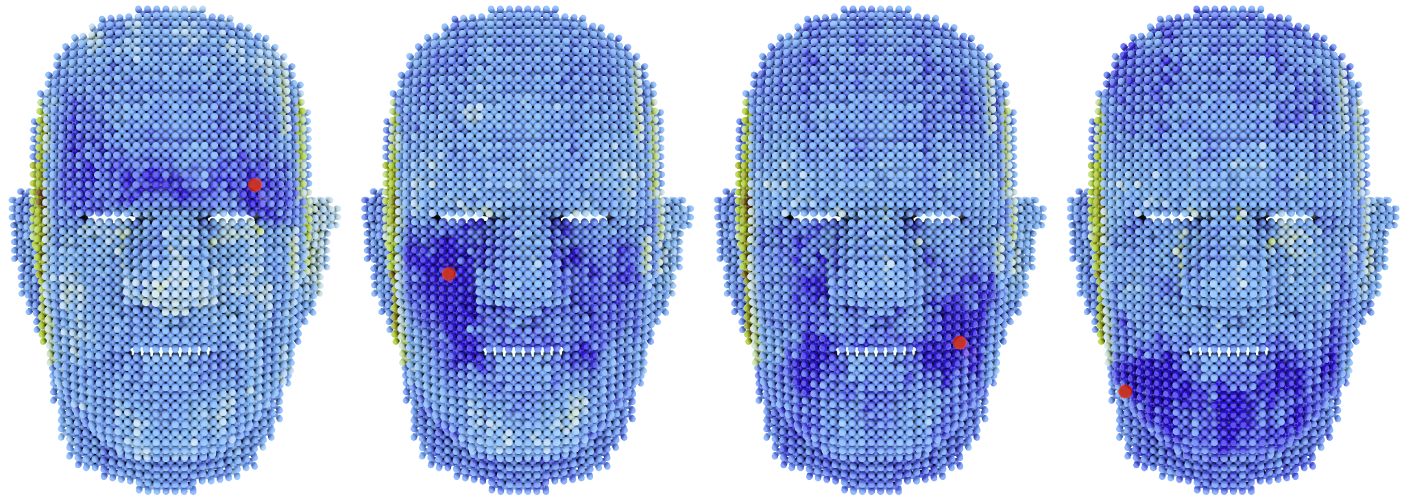
Figure 13. Correlations among different parts of the face learned in the second submodule of the Feature Encoding network. Similar colors and shades represent higher correlations with the queried (red) point.

Fig. 13 shows the learned similarities for four selected frames where the red point in each image denotes a queried point, and the similar colors and shades represent higher similarities. We observe that the Feature Encoding module has captured the correlations among different parts of the face, such as the right part of the chin being correlated with the left part of the mouth (third image from the left).

6. Conclusion

We have proposed a data-driven deep neural network framework which, using as input a low-resolution simulation of facial expression, enhances its detail and visual fidelity to levels commensurate with that of a much more expensive, high-resolution simulation. The combined performance of the low-resolution simulator and the upsampling module itself is efficient enough to yield 18.46 FPS end-to-end, with the potential of the true real-time 28.04 FPS end-to-end for a modest sacrifice of accuracy. We demonstrate that our super-resolution framework is able to convincingly bridge the visual quality gap between the real-time low-resolution and offline high-resolution simulations, even in instances where the two simulations have substantial differences due to discretization, modeling, and resolution disparities. Our super-resolution network successfully upsamples even deformations that go beyond the parametric poses exemplified in the training set (triggered by muscle action and bone motion), to include dynamics, external forces, and collision objects and constraints. Finally, we observe that our framework can approximate a degree of collision response purely via generalization from the training data. Our code is available on https://TBD

6.1. Limitations and Future Work

We have adopted a number of design choices that may consciously limit the scope of our work. We have chosen the output of our upsampling module to be the surface of the face model, rather than a description that includes the interior of the high-resolution target simulation mesh. The same output is also purely geometry, as opposed to physical quantities such as volumetric strain tensor fields or action potentials (e.g. in the style of (Srinivasan et al., 2021; Yang et al., 2022)) which might have been useful for an extra simulation pass at the high resolution to incorporate additional effects. Both such choices are made to reduce the dependency of our system on any internal traits of the simulation engine that was used to produce the high-resolution training data, requiring only surfaces at high resolution for training (those could even have originated from performance acquisition, as opposed to simulation), and stay as close to the real-time regime as possible.

Physical traits such as volume preservation, strain limits, or contact/collision behavior are only approximated to the degree that the network can learn them from data, while a full-fledged simulator could provide stronger guarantees. Specifically, if the low-resolution simulation does not employ collision handling and the high-resolution simulator used for training does, it would be very challenging to resolve behaviors where the exact result of contact resolution is history-dependent and admits multiple solutions.

As a future work, a less obvious but intriguing question is the following: if we are comfortable with the low-resolution simulation having certain modeling discrepancies from the reference high-resolution one, what might be the best constitutive model to endow the low-resolution simulation with, in order to achieve the best possible upsampling? This raises the possibility of nontrivial material coarsening approaches that more effectively condense the constitutive traits of the high-resolution model to the available scale of the low-resolution simulation – such approaches can equally well be data-driven in nature as well.

Appendix A Appendix

A.1. Additional information of our framework

A.1.1. Neural-network architecture

We report the specifications of parameters in the implemented model in Table 3, whose definitions and uses are as introduced in Sec. 3. Our model is comprised of 706,871 trainable parameters.

Table 3. Specifications of parameters in the implemented model.

Notation	Value
$N$ (num. of LR volumetric mesh vertices)	15,872
$M$ (num. HR surface mesh vertices)	35,637
S (num. of submodule layers in Feature Encoding network)	2
$D_{0}$	35
$D_{1}$	64
$D_{2}$	128
$\alpha$ in Eq. (7)	0.001
$\beta$ in Eq. (7)	gradually increased from 0.001 to 20
$k$ neighbors in the $k$-NN graphs from Feature Encoding networks	5
Interpolation neighbors for Coordinate-based Upsampling	20

A.1.2. Training Statistics

Each training epoch takes 45s on a workstation with 2 NVLink-connected NVIDIA RTX A6000 GPUs, for a batch size of 6. We trained the model for 2800 epochs (which took about 35 hours on the 2 GPU workstation). We used Adam (Kingma and Ba, 2014) to optimize the loss with a learning rate of 1e-4.

A.2. Additional information of compared models

A.2.1. Radial Basis Function (RBF)

Following the standard RBF techniques (Anjyo et al., 2014), we formulate our surface reconstruction based on RBF interpolation to predict the deformation vectors $\{\Delta\mathbf{x}^{H}_{j}\}_{j=1}^{M}$ for vertices on the HR surface mesh $\{\mathbf{x}^{H}_{j}\}_{j=1}^{M}$.

Each deformation vector of the LR mesh can be approximated as

(8) $$\Delta\mathbf{x}^{L}_{i}=\sum_{k=1}^{N}\mathbf{w}_{k}\phi(||\mathbf{x}^{L}_{i}-\mathbf{x}^{L}_{k}||),$$

where $\{\mathbf{w}_{k}\in\mathbb{R}^{3}\}$ is the set of weights we wish to find, and $\phi(||\mathbf{x}^{L}_{i}-\mathbf{x}^{L}_{k}||)\in\mathbb{R}$ is the radial function centered at $\mathbf{x}^{L}_{k}$ modeled as the Gaussian function

(9) $$\phi(R)=e^{-R^{2}/\sigma_{RBF}^{2}}.$$

We compute the distance measure $R$ geodesically following the method in Sec. 3.2. The weights $\{\mathbf{w}_{k}\}$ then can be obtained by solving the following linear system in each frame:

(10) $$\underbrace{\begin{bmatrix}\phi_{1,1}&\ldots&\phi_{1,N}\\ \vdots&\ddots&\vdots\\ \phi_{N,1}&\ldots&\phi_{N,N}\end{bmatrix}}_{=:\text{ $\Phi$}}\begin{bmatrix}\mathbf{w}^{T}_{1}\\ \vdots\\ \mathbf{w}^{T}_{N}\end{bmatrix}=\begin{bmatrix}\Delta\mathbf{x}^{L}_{1}\\ \vdots\\ \Delta\mathbf{x}^{L}_{N}\end{bmatrix},$$

where $\Phi$ is invertible for the given Gaussian radial function.

Finally, the deformation vectors $\{\Delta\mathbf{x}^{H}_{j}\}^{M}_{j=1}$ of the HR surface mesh is calculated as

(11) $$\begin{bmatrix}\Delta\mathbf{x}^{H}_{1}\\ \vdots\\ \Delta\mathbf{x}^{H}_{M}\end{bmatrix}=\begin{bmatrix}\phi(||\mathbf{x}^{H}_{1}-\mathbf{x}^{L}_{1}||)&\ldots&\phi(||\mathbf{x}^{H}_{1}-\mathbf{x}^{L}_{N}||)\\ \vdots&\ddots&\vdots\\ \phi(||\mathbf{x}^{H}_{M}-\mathbf{x}^{L}_{1}||)&\ldots&\phi(||\mathbf{x}^{H}_{M}-\mathbf{x}^{L}_{N}||)\\ \end{bmatrix}\begin{bmatrix}\mathbf{w}^{T}_{1}\\ \vdots\\ \mathbf{w}^{T}_{N}\end{bmatrix}.$$

A.2.2. Moving Least-Square (MLS)

Similarly, following the standard MLS technique for approximating scalar functions (Anjyo et al., 2014; Liu et al., 1995) we formulate our MLS-based surface reconstruction as approximating each component of displacement vectors $[\Delta x^{H}_{j},\Delta y^{H}_{j},\Delta z^{H}_{j}]\in\mathbb{R}^{3}$ for every vertex on the HR surface mesh $\{\mathbf{x}^{H}_{j}\}_{j=1}^{M}$.

The approximation is a linear combination of polynomials of degree $r$ (we use $r=2$) which, using the $y$ component (i.e., $\Delta y^{H}_{j}$) for an example, can be written as

(12) $$\Delta y^{H}_{j}=\mathbf{b}^{T}(y^{L}_{k})\mathbf{c}(\mathbf{x}^{H}_{j}),$$

where $\mathbf{b}(y)=:[1,y,y^{2},...,y^{r}]\in\mathbb{R}^{r+1}$ is the basis function, and $\mathbf{c}(\mathbf{x}^{H}_{j})=[c_{0},c_{1},...,c_{r}]\in\mathbb{R}^{r+1}$ is a vector of unknown coefficients dependent on $\mathbf{x}^{H}_{j}$, which we wish to find.

The coefficients can be obtained by solving the following weighted least-square problem:

(13) $$\mathbf{c}(\mathbf{x}^{H}_{j})=\arg\min_{\mathbf{c}\in\mathbb{R}^{r+1}}\sum_{k\in\mathcal{N}_{j}}w_{k}(||\mathbf{x}^{H}_{j}-\mathbf{x}^{L}_{k}||)\left(\mathbf{b}^{T}(y^{L}_{k})\mathbf{c}-\Delta y^{L}_{k}\right)^{2},$$

where $\mathcal{N}_{j}$ is a set of indices of LR mesh vertices neighboring $\mathbf{x}^{H}_{j}$ (we use the same 20 neighbors as defined in Sec. 3.2), and $w_{k}(D)$ is a weighting function modeled as

(14) $$w_{k}(D)=e^{-D^{2}/\sigma_{MLS}^{2}},$$

where we use the geodesic distance between $\mathbf{x}^{H}_{j}$ and $\mathbf{x}^{L}_{k}$ for the distance measure $D$ (as computed in Sec. 3.2).

Then, $\mathbf{c}(\mathbf{x}^{H}_{j})$ can be computed by differentiating Eq. (13) w.r.t. $\mathbf{c}$ and setting it to zero:

(15) $$\begin{split}&\frac{\partial}{\partial\mathbf{c}}\left(\sum_{k\in\mathcal{N}_{j}}w_{k}(||\mathbf{x}^{H}_{j}-\mathbf{x}^{L}_{k}||)\left(\mathbf{b}^{T}(y^{L}_{k})\mathbf{c}-\Delta y^{L}_{k}\right)^{2}\right)\Biggr{\rvert}_{\mathbf{c}(\mathbf{x}^{H}_{j})}=0\\ \Leftrightarrow&\underbrace{\left[\sum_{k\in\mathcal{N}_{j}}w_{k}(||\mathbf{x}^{H}_{j}-\mathbf{x}^{L}_{k}||)\mathbf{b}(y^{L}_{k})\mathbf{b}^{T}(y^{L}_{k})\right]}_{=:\text{ $M$}}\mathbf{c}(\mathbf{x}^{H}_{j})\\ &=\underbrace{\sum_{k\in\mathcal{N}_{j}}w_{k}(||\mathbf{x}^{H}_{j}-\mathbf{x}^{L}_{k}||)\Delta y^{L}_{k}\mathbf{b}(y^{L}_{k})}_{=:\text{ $\mathbf{d}$}},\end{split}$$

and solving $\mathbf{c}=M^{-1}\mathbf{d}$, where the matrix $M$ is invertible for a non-negative value of $w_{k}(D)$. For numerical stability, we re-center the polynomial basis around $\mathbf{x}^{H}_{j}$ (Liu et al., 1995), replacing $\mathbf{b}(y^{L}_{k})$ with $\mathbf{b}(y^{L}_{k}-y^{H}_{j})$ which reduces Eq. (12) to

(16) $$\Delta y^{H}_{j}=c_{0}.$$

This process is repeated for each of $x$, $y$, $z$ components (i.e., $\Delta x^{H}_{j},\Delta y^{H}_{j}$, and $\Delta z^{H}_{j}$) for every vertex on the HR mesh $\{\mathbf{x}^{H}_{j}\}^{M}_{j=1}$.

A.2.3. $\beta$-Variational Auto Encoder

We train a $\beta$-Variational Auto Encoder ($\beta$-VAE) (Higgins et al., 2016) to predict high-resolution displacements using low-resolution displacements as input to serve as a baseline generative neural network. The $\beta$-VAE has 2 fully connected layers in the encoder and 3 fully connected layers in the decoder. The encoder has 2 hidden layers with 1024 neurons in the first layer and 512 neurons in the second layer. The output of the encoder is composed of 256 neurons (128 neurons for the mean and 128 neurons for the variance). The decoder has 3 hidden layers with 256, 1024, and 4096 neurons. All the hidden layers use Leaky RELU activations. During every training epoch, the mean and variance output from the encoder are used to compute latent parameters by sampling from a normal distribution. To train the weights of this network, we compute the loss on the output displacements (L2-norm) and the KL-Divergence of the latent parameters. The former penalizes reconstruction error while the latter encourages disentanglement between latent parameters. The KL-Divergence term is also scaled by a hyperparameter $\beta$ which controls the degree of disentanglement between the latent parameters. We fixed $\beta$ to be 0.01 for this dataset and used Adam (Kingma and Ba, 2014) to train the network weights, with a learning rate of 1e-4. Since the input and output dimensions of our $\beta$-VAE are different, we do not design identical encoder and decoder architectures. We use the same partition for the train and test sets as our method.

A.2.4. Deep Detail Enhancement framework

We compare with Deep Detail Enhancement (DDE) framework (Zhang et al., 2021) as the representative state-of-the-art method for synthesizing plausible wrinkle details on a coarse garment geometry based on normal maps. For implementation, we first bake two UV normal maps of size 512$\times$512 for each of the surface mesh embedded in the low-resolution (LR) simulation mesh (e.g., left image of Fig. 5) and the surface conforming to the high-resolution (HR) simulation mesh (e.g., right image of Fig. 5) on a frame-by-frame basis. Then, we train the DDE network (with U-Net architecture) to predict the HR normal map from its LR counterpart, baked from the training dataset. We train on the full-size normal maps rather than randomly subsampled patches as in the original work and omit training of the garment material classifier since we have only one type of mesh, the face. Also, we added one layers of downsampling and upsampling, respectively, given our input dimension is larger compared to the original work (128$\times$128) and also follow the same energy-minimization method to recover 3D surfaces from the normal maps, initialized with the coarse embedded mesh.

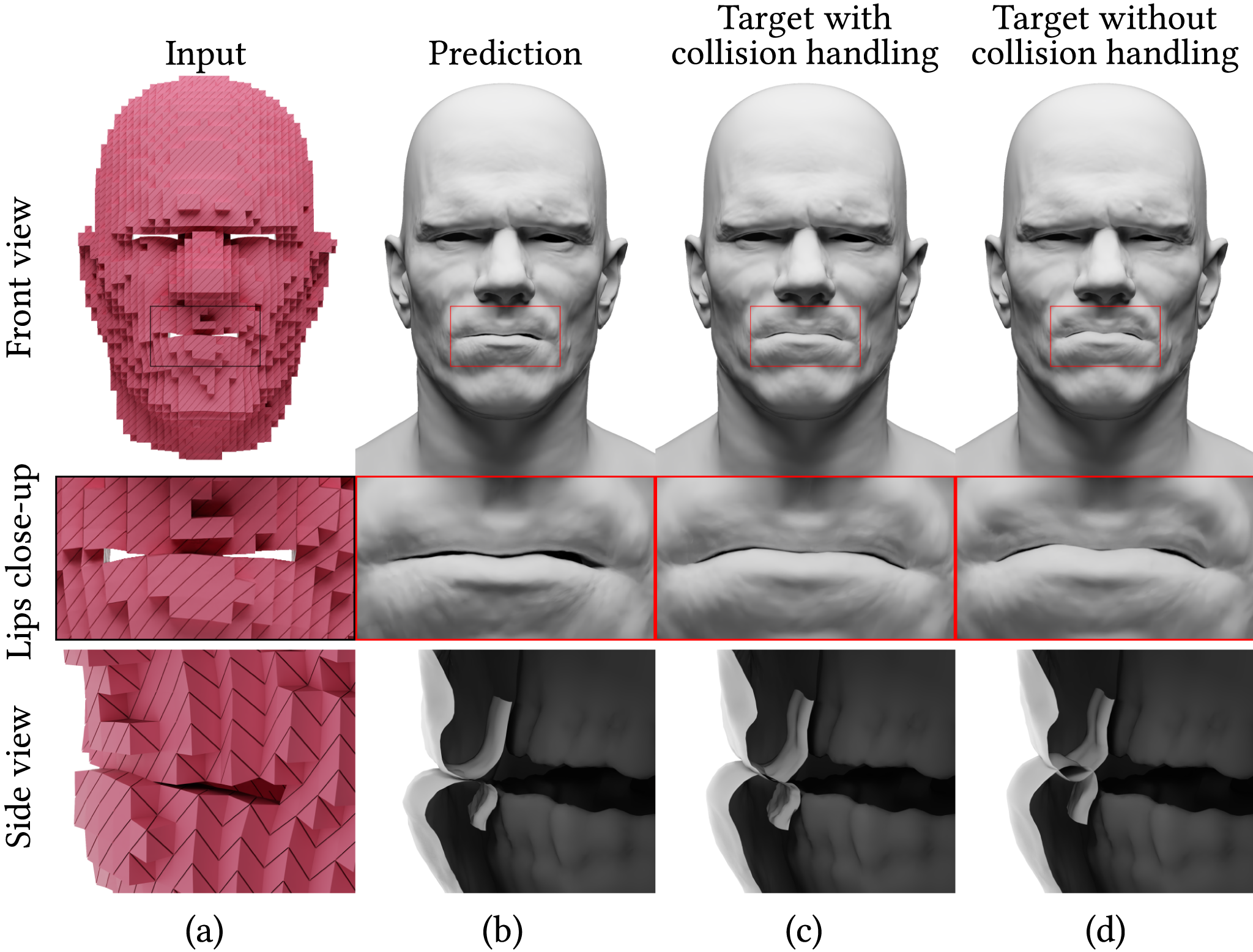
[r] Nvidia^©

Figure 14. An example of complete collision resolution: The prediction of our framework (b) on a test performance (a) has collisions resolved. The performance (when simulated in high resolution) with and without collision handling is shown in (c) and (d), respectively. Notice that when the penetration is low, collisions are resolved in the prediction.

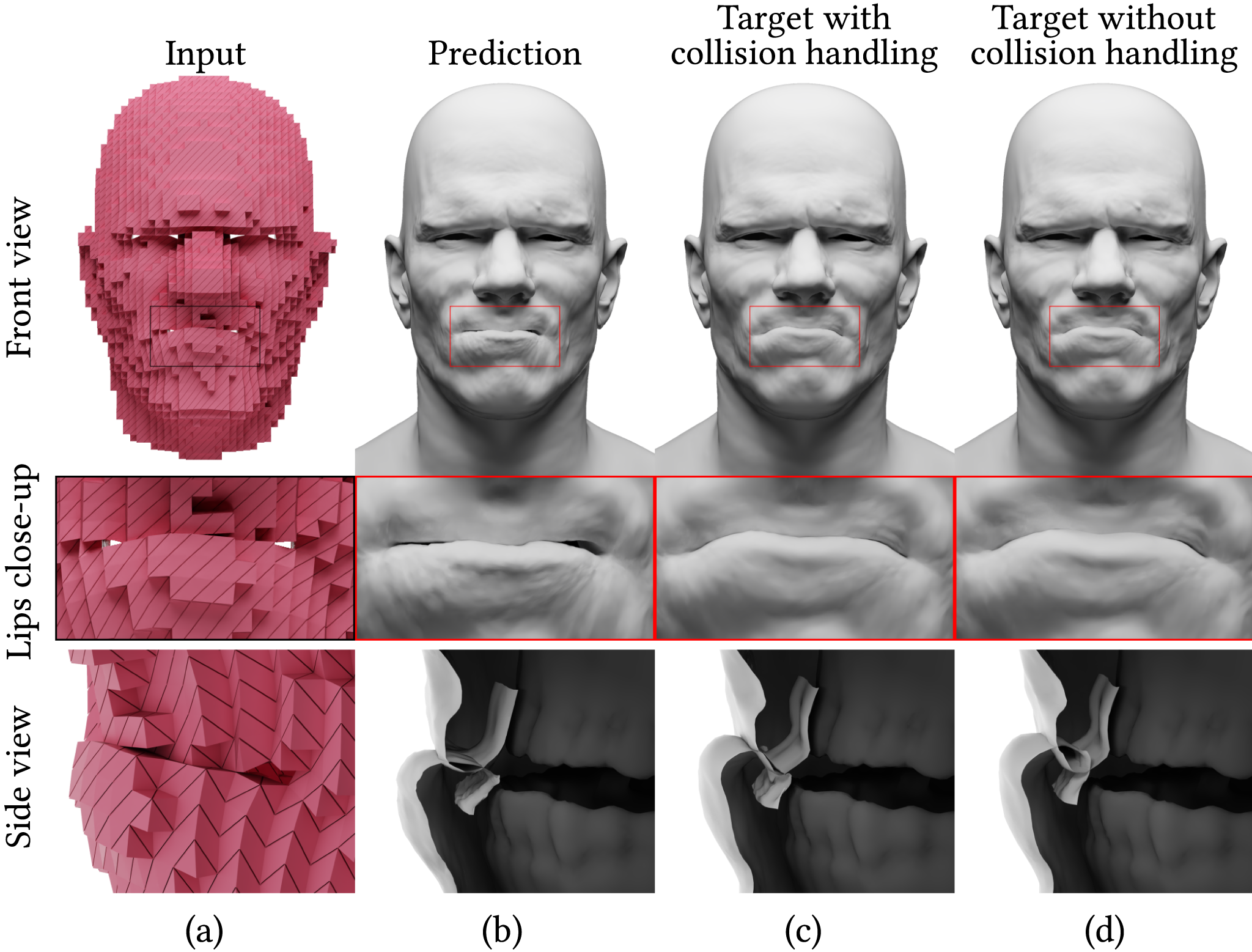
[r] Nvidia^©

Figure 15. An example of partial collision resolution: The prediction of our framework (b) on a test performance (a) has collisions partially resolved. The performance (when simulated in high resolution) with and without collision handling is shown in (c) and (d), respectively. Notice that when the penetration is higher, collisions are partially resolved in the prediction.

A.2.5. Approximate resolution of self-collision

We validate the qualitative performance of self-collisions by visualizing and comparing the predictions on the test set with two variants of the high-resolution surface, collision handling applied in the simulation (Figures 14c and 15c) and omitted in the simulation (Figures 14d and 15d). As mentioned in Sec. 4, we do not resolve self-collisions in the low-resolution simulations, but only in the high-resolution simulations. We notice that the model can partially resolve self-collisions depending on the degree of collision (or penetration). Fig. 14 illustrates one such test set performance where the prediction from our model (Fig. 14b) does not have lip self-collisions when the penetration is low (Fig. 14d). Conversely, when the penetration is high, as shown in Fig. 15d, the prediction has collisions partially resolved (Fig. 15b). We also highlight that we do not add any additional penalty for collisions during training and the model has learned this from the training data performances alone.

References

- (1)
- Alexa et al. (2001) Marc Alexa, Johannes Behr, Daniel Cohen-Or, Shachar Fleishman, David Levin, and Claudio T Silva. 2001. Point set surfaces. In Proceedings Visualization, 2001. VIS’01. IEEE, 21–29.
- Alexa et al. (2003) Marc Alexa, Johannes Behr, Daniel Cohen-Or, Shachar Fleishman, David Levin, and Claudio T. Silva. 2003. Computing and rendering point set surfaces. IEEE Transactions on visualization and computer graphics 9, 1 (2003), 3–15.
- Ali-Hamadi et al. (2013) Dicko Ali-Hamadi, Tiantian Liu, Benjamin Gilles, Ladislav Kavan, François Faure, Olivier Palombi, and Marie-Paule Cani. 2013. Anatomy Transfer. ACM Trans. Graph. 32, 6, Article 188 (nov 2013), 8 pages. https://doi.org/10.1145/2508363.2508415
- Anjyo et al. (2014) Ken Anjyo, John P Lewis, and Frédéric Pighin. 2014. Scattered data interpolation for computer graphics. In ACM SIGGRAPH 2014 Courses. 1–69.
- Bailey et al. (2020) Stephen W Bailey, Dalton Omens, Paul Dilorenzo, and James F O’Brien. 2020. Fast and deep facial deformations. ACM Transactions on Graphics (TOG) 39, 4 (2020), 94–1.
- Bao et al. (2019) Michael Bao, Matthew Cong, Stéphane Grabli, and Ronald Fedkiw. 2019. High-quality face capture using anatomical muscles. In Proceedings of the IEEE/CVF Conference on Computer Vision and Pattern Recognition. 10802–10811.
- Bender et al. (2013) Jan Bender, Matthias Müller, Miguel A Otaduy, and Matthias Teschner. 2013. Position-based Methods for the Simulation of Solid Objects in Computer Graphics.. In Eurographics (State of the Art Reports). 1–22.
- Berger et al. (2017) Matthew Berger, Andrea Tagliasacchi, Lee M Seversky, Pierre Alliez, Gael Guennebaud, Joshua A Levine, Andrei Sharf, and Claudio T Silva. 2017. A survey of surface reconstruction from point clouds. In Computer Graphics Forum, Vol. 36. Wiley Online Library, 301–329.
- Bergou et al. (2007) Miklós Bergou, Saurabh Mathur, Max Wardetzky, and Eitan Grinspun. 2007. Tracks: toward directable thin shells. ACM Transactions on Graphics (TOG) 26, 3 (2007), 50–es.
- Berretti et al. (2012) Stefano Berretti, Alberto Del Bimbo, and Pietro Pala. 2012. Superfaces: A super-resolution model for 3D faces. In European Conference on Computer Vision. Springer, 73–82.
- Berretti et al. (2014) Stefano Berretti, Pietro Pala, and Alberto Del Bimbo. 2014. Face recognition by super-resolved 3D models from consumer depth cameras. IEEE transactions on information forensics and security 9, 9 (2014), 1436–1449.
- Bondi et al. (2016) Enrico Bondi, Pietro Pala, Stefano Berretti, and Alberto Del Bimbo. 2016. Reconstructing high-resolution face models from kinect depth sequences. IEEE Transactions on Information Forensics and Security 11, 12 (2016), 2843–2853.
- Bouaziz et al. (2014) Sofien Bouaziz, Sebastian Martin, Tiantian Liu, Ladislav Kavan, and Mark Pauly. 2014. Projective dynamics: Fusing constraint projections for fast simulation. ACM transactions on graphics (TOG) 33, 4 (2014), 1–11.
- Carr et al. (2001) Jonathan C Carr, Richard K Beatson, Jon B Cherrie, Tim J Mitchell, W Richard Fright, Bruce C McCallum, and Tim R Evans. 2001. Reconstruction and representation of 3D objects with radial basis functions. In Proceedings of the 28th annual conference on Computer graphics and interactive techniques. 67–76.
- Chabra et al. (2020) Rohan Chabra, Jan E Lenssen, Eddy Ilg, Tanner Schmidt, Julian Straub, Steven Lovegrove, and Richard Newcombe. 2020. Deep local shapes: Learning local sdf priors for detailed 3d reconstruction. In European Conference on Computer Vision. Springer, 608–625.
- Chan et al. (2021) Eric R Chan, Marco Monteiro, Petr Kellnhofer, Jiajun Wu, and Gordon Wetzstein. 2021. pi-gan: Periodic implicit generative adversarial networks for 3d-aware image synthesis. In Proceedings of the IEEE/CVF conference on computer vision and pattern recognition. 5799–5809.
- Chen et al. (2021) Yinbo Chen, Sifei Liu, and Xiaolong Wang. 2021. Learning continuous image representation with local implicit image function. In Proceedings of the IEEE/CVF conference on computer vision and pattern recognition. 8628–8638.
- Choi and Blemker (2013) Hon Fai Choi and Silvia S. Blemker. 2013. Skeletal Muscle Fascicle Arrangements Can Be Reconstructed Using a Laplacian Vector Field Simulation. PLOS ONE 8, 10 (10 2013), 1–7. https://doi.org/10.1371/journal.pone.0077576
- Cong et al. (2015) Matthew Cong, Michael Bao, Jane L E, Kiran S Bhat, and Ronald Fedkiw. 2015. Fully automatic generation of anatomical face simulation models. In Proceedings of the 14th ACM SIGGRAPH/Eurographics Symposium on Computer Animation. 175–183.
- Cong et al. (2016) Matthew Cong, Kiran S. Bhat, and Ronald Fedkiw. 2016. Art-Directed Muscle Simulation for High-End Facial Animation. In Proceedings of the ACM SIGGRAPH/Eurographics Symposium on Computer Animation (Zurich, Switzerland) (SCA ’16). Eurographics Association, Goslar, DEU, 119–127.
- Crouse (2016) David F Crouse. 2016. On implementing 2D rectangular assignment algorithms. IEEE Trans. Aerospace Electron. Systems 52, 4 (2016), 1679–1696.
- Curless and Levoy (1996) Brian Curless and Marc Levoy. 1996. A volumetric method for building complex models from range images. In Proceedings of the 23rd annual conference on Computer graphics and interactive techniques. 303–312.
- Fleishman et al. (2005) Shachar Fleishman, Daniel Cohen-Or, and Cláudio T Silva. 2005. Robust moving least-squares fitting with sharp features. ACM transactions on graphics (TOG) 24, 3 (2005), 544–552.
- Hauth and Etzmuss (2001) Michael Hauth and Olaf Etzmuss. 2001. A high performance solver for the animation of deformable objects using advanced numerical methods. In Computer Graphics Forum, Vol. 20. Wiley Online Library, 319–328.
- Higgins et al. (2016) Irina Higgins, Loic Matthey, Arka Pal, Christopher Burgess, Xavier Glorot, Matthew Botvinick, Shakir Mohamed, and Alexander Lerchner. 2016. beta-vae: Learning basic visual concepts with a constrained variational framework. (2016).
- Jiang et al. (2020) Chiyu Jiang, Avneesh Sud, Ameesh Makadia, Jingwei Huang, Matthias Nießner, Thomas Funkhouser, et al. 2020. Local implicit grid representations for 3d scenes. In Proceedings of the IEEE/CVF Conference on Computer Vision and Pattern Recognition. 6001–6010.
- Kazhdan et al. (2006) Michael Kazhdan, Matthew Bolitho, and Hugues Hoppe. 2006. Poisson surface reconstruction. In Proceedings of the fourth Eurographics symposium on Geometry processing, Vol. 7.
- Kazhdan and Hoppe (2013) Michael Kazhdan and Hugues Hoppe. 2013. Screened poisson surface reconstruction. ACM Transactions on Graphics (ToG) 32, 3 (2013), 1–13.
- Kharevych et al. (2006) Liliya Kharevych, W Wei, Yiying Tong, Eva Kanso, Jerrold E Marsden, Peter Schröder, and Matthieu Desbrun. 2006. Geometric, variational integrators for computer animation. Eurographics Association.
- Kim et al. (2008) Theodore Kim, Nils Thürey, Doug James, and Markus Gross. 2008. Wavelet turbulence for fluid simulation. ACM Transactions on Graphics (TOG) 27, 3 (2008), 1–6.
- Kingma and Ba (2014) Diederik P. Kingma and Jimmy Ba. 2014. Adam: A Method for Stochastic Optimization. https://doi.org/10.48550/ARXIV.1412.6980
- Li et al. (2021) Jiaxin Li, Feiyu Zhu, Xiao Yang, and Qijun Zhao. 2021. 3D face point cloud super-resolution network. In 2021 IEEE International Joint Conference on Biometrics (IJCB). IEEE, 1–8.
- Li et al. (2019) Ruihui Li, Xianzhi Li, Chi-Wing Fu, Daniel Cohen-Or, and Pheng-Ann Heng. 2019. Pu-gan: a point cloud upsampling adversarial network. In Proceedings of the IEEE/CVF international conference on computer vision. 7203–7212.
- Liang et al. (2014) Shu Liang, Ira Kemelmacher-Shlizerman, and Linda G Shapiro. 2014. 3d face hallucination from a single depth frame. In 2014 2nd International Conference on 3D Vision, Vol. 1. IEEE, 31–38.
- Liu et al. (2013) Tiantian Liu, Adam W Bargteil, James F O’Brien, and Ladislav Kavan. 2013. Fast simulation of mass-spring systems. ACM Transactions on Graphics (TOG) 32, 6 (2013), 1–7.
- Liu et al. (1995) Wing Kam Liu, Sukky Jun, and Yi Fei Zhang. 1995. Reproducing kernel particle methods. International journal for numerical methods in fluids 20, 8-9 (1995), 1081–1106.
- Ma et al. (2021) Shugao Ma, Tomas Simon, Jason Saragih, Dawei Wang, Yuecheng Li, Fernando De La Torre, and Yaser Sheikh. 2021. Pixel codec avatars. In Proceedings of the IEEE/CVF Conference on Computer Vision and Pattern Recognition. 64–73.
- Macklin et al. (2016) Miles Macklin, Matthias Müller, and Nuttapong Chentanez. 2016. XPBD: position-based simulation of compliant constrained dynamics. In Proceedings of the 9th International Conference on Motion in Games. 49–54.
- Mescheder et al. (2019) Lars Mescheder, Michael Oechsle, Michael Niemeyer, Sebastian Nowozin, and Andreas Geiger. 2019. Occupancy networks: Learning 3d reconstruction in function space. In Proceedings of the IEEE/CVF conference on computer vision and pattern recognition. 4460–4470.
- Mildenhall et al. (2021) Ben Mildenhall, Pratul P Srinivasan, Matthew Tancik, Jonathan T Barron, Ravi Ramamoorthi, and Ren Ng. 2021. Nerf: Representing scenes as neural radiance fields for view synthesis. Commun. ACM 65, 1 (2021), 99–106.
- Molino et al. (2003) Neil Molino, Robert Bridson, Joseph Teran, and Ronald Fedkiw. 2003. A crystalline, red green strategy for meshing highly deformable objects with tetrahedra.. In IMR. Citeseer, 103–114.
- Müller et al. (2007) Matthias Müller, Bruno Heidelberger, Marcus Hennix, and John Ratcliff. 2007. Position based dynamics. Journal of Visual Communication and Image Representation 18, 2 (2007), 109–118.
- Nagai et al. (2009) Yukie Nagai, Yutaka Ohtake, and Hiromasa Suzuki. 2009. Smoothing of partition of unity implicit surfaces for noise robust surface reconstruction. In Computer Graphics Forum, Vol. 28. Wiley Online Library, 1339–1348.
- Nasrollahi and Moeslund (2014) Kamal Nasrollahi and Thomas B Moeslund. 2014. Super-resolution: a comprehensive survey. Machine vision and applications 25, 6 (2014), 1423–1468.
- Ohtake et al. (2005a) Yutaka Ohtake, Alexander Belyaev, and Marc Alexa. 2005a. Sparse low-degree implicit surfaces with applications to high quality rendering, feature extraction, and smoothing. In Proc. Symp. Geometry Processing. 149–158.
- Ohtake et al. (2005b) Yutaka Ohtake, Alexander Belyaev, and Hans-Peter Seidel. 2005b. 3D scattered data interpolation and approximation with multilevel compactly supported RBFs. Graphical Models 67, 3 (2005), 150–165.
- Pan et al. (2006) Gang Pan, Shi Han, Zhaohui Wu, and Yueming Wang. 2006. Super-resolution of 3d face. In European Conference on Computer Vision. Springer, 389–401.
- Park et al. (2019) Jeong Joon Park, Peter Florence, Julian Straub, Richard Newcombe, and Steven Lovegrove. 2019. Deepsdf: Learning continuous signed distance functions for shape representation. In Proceedings of the IEEE/CVF conference on computer vision and pattern recognition. 165–174.
- Peng et al. (2005) Shiqi Peng, Gang Pan, and Zhaohui Wu. 2005. Learning-based super-resolution of 3D face model. In IEEE International Conference on Image Processing 2005, Vol. 2. IEEE, II–382.
- Qian et al. (2021) Guocheng Qian, Abdulellah Abualshour, Guohao Li, Ali Thabet, and Bernard Ghanem. 2021. Pu-gcn: Point cloud upsampling using graph convolutional networks. In Proceedings of the IEEE/CVF Conference on Computer Vision and Pattern Recognition. 11683–11692.
- Qian et al. (2020) Yue Qian, Junhui Hou, Sam Kwong, and Ying He. 2020. PUGeo-Net: A geometry-centric network for 3D point cloud upsampling. In European conference on computer vision. Springer, 752–769.
- Saito et al. (2019) Shunsuke Saito, Zeng Huang, Ryota Natsume, Shigeo Morishima, Angjoo Kanazawa, and Hao Li. 2019. Pifu: Pixel-aligned implicit function for high-resolution clothed human digitization. In Proceedings of the IEEE/CVF International Conference on Computer Vision. 2304–2314.
- Sifakis et al. (2005) Eftychios Sifakis, Igor Neverov, and Ronald Fedkiw. 2005. Automatic determination of facial muscle activations from sparse motion capture marker data. In ACM SIGGRAPH 2005 Papers. 417–425.
- Sitzmann et al. (2020) Vincent Sitzmann, Julien Martel, Alexander Bergman, David Lindell, and Gordon Wetzstein. 2020. Implicit neural representations with periodic activation functions. Advances in Neural Information Processing Systems 33 (2020), 7462–7473.
- Srinivasan et al. (2021) Sangeetha Grama Srinivasan, Qisi Wang, Junior Rojas, Gergely Klár, Ladislav Kavan, and Eftychios Sifakis. 2021. Learning active quasistatic physics-based models from data. ACM Transactions on Graphics (TOG) 40, 4 (2021), 1–14.
- Stam (2009) Jos Stam. 2009. Nucleus: Towards a unified dynamics solver for computer graphics. In 2009 11th IEEE International Conference on Computer-Aided Design and Computer Graphics. IEEE, 1–11.
- Stern and Grinspun (2009) Ari Stern and Eitan Grinspun. 2009. Implicit-explicit variational integration of highly oscillatory problems. Multiscale Modeling & Simulation 7, 4 (2009), 1779–1794.
- Su et al. (2013) Jonathan Su, Rahul Sheth, and Ronald Fedkiw. 2013. Energy conservation for the simulation of deformable bodies. IEEE Trans. Vis. Comput. Graph. 19, 2 (2013), 189–200.
- Tancik et al. (2020) Matthew Tancik, Pratul Srinivasan, Ben Mildenhall, Sara Fridovich-Keil, Nithin Raghavan, Utkarsh Singhal, Ravi Ramamoorthi, Jonathan Barron, and Ren Ng. 2020. Fourier features let networks learn high frequency functions in low dimensional domains. Advances in Neural Information Processing Systems 33 (2020), 7537–7547.
- Teran et al. (2003) Joseph Teran, Sylvia Blemker, V Ng Thow Hing, and Ronald Fedkiw. 2003. Finite volume methods for the simulation of skeletal muscle. In Proceedings of the 2003 ACM SIGGRAPH/Eurographics symposium on Computer animation. 68–74.
- Teran et al. (2005) Joseph Teran, Eftychios Sifakis, Geoffrey Irving, and Ronald Fedkiw. 2005. Robust quasistatic finite elements and flesh simulation. In Proceedings of the 2005 ACM SIGGRAPH/Eurographics symposium on Computer animation. 181–190.
- Turk and O’brien (2002) Greg Turk and James F O’brien. 2002. Modelling with implicit surfaces that interpolate. ACM Transactions on Graphics (TOG) 21, 4 (2002), 855–873.
- Vaswani et al. (2017) Ashish Vaswani, Noam Shazeer, Niki Parmar, Jakob Uszkoreit, Llion Jones, Aidan N Gomez, Łukasz Kaiser, and Illia Polosukhin. 2017. Attention is all you need. Advances in neural information processing systems 30 (2017).
- Wang et al. (2019) Yue Wang, Yongbin Sun, Ziwei Liu, Sanjay E Sarma, Michael M Bronstein, and Justin M Solomon. 2019. Dynamic graph cnn for learning on point clouds. Acm Transactions On Graphics (tog) 38, 5 (2019), 1–12.
- Xie et al. (2018) You Xie, Erik Franz, Mengyu Chu, and Nils Thuerey. 2018. tempoGAN: A temporally coherent, volumetric GAN for super-resolution fluid flow. ACM Transactions on Graphics (TOG) 37, 4 (2018), 1–15.
- Yang et al. (2022) Lingchen Yang, Byungsoo Kim, Gaspard Zoss, Baran Gözcü, Markus Gross, and Barbara Solenthaler. 2022. Implicit neural representation for physics-driven actuated soft bodies. ACM Transactions on Graphics (TOG) 41, 4 (2022), 1–10.
- Yang et al. (2019) Wenming Yang, Xuechen Zhang, Yapeng Tian, Wei Wang, Jing-Hao Xue, and Qingmin Liao. 2019. Deep learning for single image super-resolution: A brief review. IEEE Transactions on Multimedia 21, 12 (2019), 3106–3121.
- Ye et al. (2021) Shuquan Ye, Dongdong Chen, Songfang Han, Ziyu Wan, and Jing Liao. 2021. Meta-PU: An arbitrary-scale upsampling network for point cloud. IEEE transactions on visualization and computer graphics (2021).
- Yifan et al. (2019) Wang Yifan, Shihao Wu, Hui Huang, Daniel Cohen-Or, and Olga Sorkine-Hornung. 2019. Patch-based progressive 3d point set upsampling. In Proceedings of the IEEE/CVF Conference on Computer Vision and Pattern Recognition. 5958–5967.
- Yu et al. (2018a) Lequan Yu, Xianzhi Li, Chi-Wing Fu, Daniel Cohen-Or, and Pheng-Ann Heng. 2018a. Ec-net: an edge-aware point set consolidation network. In Proceedings of the European conference on computer vision (ECCV). 386–402.
- Yu et al. (2018b) Lequan Yu, Xianzhi Li, Chi-Wing Fu, Daniel Cohen-Or, and Pheng-Ann Heng. 2018b. Pu-net: Point cloud upsampling network. In Proceedings of the IEEE conference on computer vision and pattern recognition. 2790–2799.
- Zhang et al. (2020) Fan Zhang, Junli Zhao, Liang Wang, and Fuqing Duan. 2020. 3d face model super-resolution based on radial curve estimation. Applied Sciences 10, 3 (2020), 1047.
- Zhang et al. (2021) Meng Zhang, Tuanfeng Wang, Duygu Ceylan, and Niloy J Mitra. 2021. Deep detail enhancement for any garment. In Computer Graphics Forum, Vol. 40. Wiley Online Library, 399–411.
- Zhang et al. (2022) Yan Zhang, Wenhan Zhao, Bo Sun, Ying Zhang, and Wen Wen. 2022. Point Cloud Upsampling Algorithm: A Systematic Review. Algorithms 15, 4 (2022), 124.
- Zurdo et al. (2012) Javier S Zurdo, Juan P Brito, and Miguel A Otaduy. 2012. Animating wrinkles by example on non-skinned cloth. IEEE Transactions on Visualization and Computer Graphics 19, 1 (2012), 149–158.