Debiased Inference for Dynamic Nonlinear Models with Two-way Fixed Effects

Abstract

Panel data models often use fixed effects to account for unobserved heterogeneities. These fixed effects are typically incidental parameters and their estimators converge slowly relative to the square root of the sample size. In the maximum likelihood context, this induces an asymptotic bias of the likelihood function. Test statistics derived from the asymptotically biased likelihood, therefore, no longer follow their standard limiting distributions. This causes severe distortions in test sizes. We consider a generic class of dynamic nonlinear models with two-way fixed effects and propose an analytical bias correction method for the likelihood function. We formally show that the likelihood ratio, the Lagrange-multiplier, and the Wald test statistics derived from the corrected likelihood follow their standard asymptotic distributions. A bias-corrected estimator of the structural parameters can also be derived from the corrected likelihood function. We evaluate the performance of our bias correction procedure through simulations and an empirical example.

Keywords: analytical bias correction, dynamic panel models, incidental parameter problem, two-way fixed effects
JEL Classification C23

1 Introduction

Panel data, also known as longitudinal data, is common in empirical studies where observations are collected from $N$ individuals over a span of $T$ time periods. These data sets often contain unobserved heterogeneities specific to individuals or time periods which can be correlated with the covariates in a regression context. To account for such unobserved heterogeneities, a standard technique is to use two-way fixed effects, where individual and time effects are included for every individual $i=1,\ldots,N$ and every time period $t=1,\ldots,T$.

Unlike linear models, however, the usual technique of within transformation is generally not applicable to nonlinear maximum likelihood models, and the estimation of the fixed effects is often inevitable. Such an estimation induces the incidental parameter problem (IPP) of Neyman and Scott (1948) in the sense that the estimators of the fixed effects contaminate the likelihood function. See Lancaster (2000) and Fernández-Val and Weidner (2018) for recent reviews. Under a large $N,T$ asymptotics, the estimators of individual and time effects converge at a rate of, respectively, $1/\sqrt{T}$ and $1/\sqrt{N}$. These slow rates of convergence cause the asymptotic distribution of the likelihood function, evaluated at the estimated effects, to have a non-zero center and exhibit bias. Consequently, many likelihood-based test statistics inherit such a bias and no longer follow their standard asymptotic distributions, leading to incorrect test sizes. In particular, the likelihood-ratio (LR), the Lagrangian-multiplier (LM), and the Wald test statistics are no longer $\chi^{2}$-distributed under the null (about the true value of the structural parameter, $\theta_{0}$). It is worth noting that such an asymptotic bias would become negligible under $N/T\rightarrow 0$ as $N,T\rightarrow\infty$, if the model included only the individual effects; or under $N/T\rightarrow\infty$ as $N,T\rightarrow\infty$, if the model only included the time effects. However, when the model includes both effects, there is no such relative rate $N/T$ under which the bias becomes negligible, and certain procedures have to be employed to correct the bias. In this paper, we consider a generic class of dynamic nonlinear models with two-way fixed effects and develop a bias-corrected likelihood free of the asymptotic bias under $N,T\rightarrow\infty$ where $N$ and $T$ grow proportionally. Our bias-corrected likelihood essentially approximates an IPP-free infeasible likelihood in the sense of profiled likelihoods (see, e.g., Pace and Salvan (2006)). We formally prove that the LR, the LM, and the Wald test statistics are all asymptotically $\chi^{2}$ under the null when they are derived from our corrected likelihood.

Figure 1 illustrates the consequences of the IPP in test statistics for logit models. The figure displays the simulated rejection rates of the LR test, with a significance level of 5%, under a range of null hypotheses about $\theta_{0}$. The rejection rates are calculated using different likelihood functions: i) an infeasible likelihood that is free of the IPP, ii) the original (contaminated) likelihood that is affected by the IPP, and iii) the bias-corrected likelihood that we develop. The precise definition of these likelihood functions will become clear as we proceed. The plotted curves show that the LR test using the original likelihood severely over-rejects the true null hypothesis at $\theta_{0}$, with rejection rates approaching ${20\%}$ for both the dynamic and static logit models. This is the IPP in the context of hypothesis testing, and it arises due to the inclusion of the estimated two-way effects in the original likelihood. The LM and Wald tests using the original likelihood also suffer from the IPP. On the other hand, the LR test using the infeasible likelihood delivers rejection rates very close to the nominal level of $5\%$ at $\theta_{0}$ for both the dynamic and static models. Our bias-corrected likelihood produces a rejection rate close to the nominal level of $5\%$ at $\theta_{0}$. The performance is comparable to the infeasible likelihood.

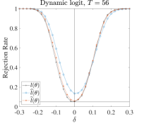
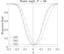
Figure 1: Size and power of LR tests for logit model with $\alpha_{i}U_{it}+\gamma_{t}V_{it}$

Notes: The plotted curves are the rejection rates of the LR tests based on an infeasible likelihood $l\left(\theta\right)$, the original likelihood $\widehat{l}\left(\theta\right)$, as well as our corrected likelihood function $\widetilde{l}\left(\theta\right)$. They are all profiled likelihood functions whose exact definitions will become clear as we proceed. The dynamic model is $Y_{it}=1(\rho_{0}Y_{it-1}+\beta_{0}X_{it}+\alpha_{i0}U_{it}+\gamma_{t0}V_{it}+\varepsilon_{it}>0)$ and the static model is $Y_{it}=1(\beta_{0}X_{it}+\alpha_{i0}U_{it}+\gamma_{t0}V_{it}+\varepsilon_{it})>0$, where ${1}\left(\cdot\right)$ is the indicator function, $X_{it}=X_{it-1}/2+\alpha_{i0}+\gamma_{t0}+\nu_{it}$ with $\nu_{it}\sim\mathcal{N}\left(0,1/2\right)$, and $\varepsilon_{it}$ is standard logistic. $U_{it}$ and $V_{it}$ are generated in the same way as $X_{it}$. Other details are given in Section 4. The true value of structural parameter $\theta_{0}=\left(\rho_{0},\beta_{0}\right)^{\prime}=\left(0.5,1\right)^{\prime}$ for the dynamic model and $\theta_{0}={\beta_{0}=1}$ for the static. The null is at $\theta_{0}+\delta$ where, as depicted on the horizontal axis, $\delta\in\left\{-0.3,0.28,\cdots,0.3\right\}$. The vertical line is at the true value and the horizontal at the significance level $5\%$.

Several papers in the literature on the IPP in the presence of two-way fixed effects are closely related to our method. For example, Fernández-Val and Weidner (2016) propose a bias correction method for the maximum likelihood estimator (MLE) of a generic class of nonlinear dynamic model with two-way additive effects. See also Chen et al. (2021) for a similar approach for interactive effects. Both approaches of Fernández-Val and Weidner (2016) and Chen et al. (2021) are “parameter-based” in the sense that they develop formulas for the asymptotic bias of the MLE. However, bias corrections of the MLE do not generally lead to bias corrections of the likelihood or its related objects. For instance, the LR test statistic generally does not follow a $\chi^{2}$-distribution under the null, even when evaluated at the bias-corrected MLE. This paper differs from Fernández-Val and Weidner (2016) and Chen et al. (2021) in that our approach is “likelihood-based” as the correction applies to the likelihood function itself. This benefits objects in the entire likelihood hierarchy. In this paper, the objects of interest are the LR, the LM, and the Wald test statistics.

In addition to this, we accommodate a wider class of models where the two-way effects enter the model in general, and potentially non-additive, ways. A particular class is the recent heterogeneous slope coefficient model. In such a model, the slope coefficients may depend on both $i$ and $t$, due to unobserved heterogeneities in both dimensions. For instance, the slope coefficient may be given by $\beta_{it}=\beta+\alpha_{i}+\gamma_{t}$ (see, e.g., Keane and Neal (2020)) or $\beta_{it}=\beta(\alpha_{i}+\gamma_{t})$ (see, e.g., Lu and Su (2023) and Hahn et al. (2023)). The heterogeneous slope coefficient model is useful in many empirical works as it allows for richer forms of heterogeneities compared to the traditional “heterogeneous intercept” model. However, such models are generally subject to the incidental parameter problem as well, and bias correction procedures are not yet well-discussed.

Our procedure is similar to Jochmans and Otsu (2019), who also develop a likelihood-based bias correction method. In fact, Jochmans and Otsu (2019) already show using simulations that the LR, the LM, and the Wald test all benefit from their corrected likelihood with reduced size distortions. However, Jochmans and Otsu (2019) only consider models with strictly exogenous regressors, whereas we allow for predetermined regressors as well. Beyond this point, we also provide formal proofs for the asymptotic properties of the corrected likelihood and of the derived LR, the LM, and the Wald statistics under relatively mild regularity conditions. Amongst other things, we formally establish that the profiled score inherits the bias correction of the likelihood. This seems to be missing in the current relevant literature but can be important for the general understanding of the behaviors of the bias-corrected likelihood and its derived objects.

Other works for models with two-way fixed effects include Hahn and Moon (2006), Bai (2009), Bai (2013), Moon and Weidner (2015), Charbonneau (2017), and Hong et al. (2022). For models with individual effects only, the literature is extensive. For instance, Rasch (1961), Andersen (1970), Chamberlain (1980), Arellano and Bond (1991), and Lancaster (2002) provide solutions that eliminate the IPP under fixed $T$ for rather narrow classes of models. Several bias correction methods are also available. They do not eliminate the IPP bias but provide asymptotically unbiased MLE under $N,T\rightarrow\infty$ jointly where $N/T\rightarrow\infty$. They include Hahn and Kuersteiner (2002), Hahn and Newey (2004), and Hahn and Kuersteiner (2011) which are parameter-based; and Dhaene and Jochmans (2015b), Arellano and Hahn (2016), Dhaene and Sun (2021), and Schumann (2022) which are likelihood-based. In addition, Sartori (2003), Arellano and Bonhomme (2009), and De Bin et al. (2015) achieve bias corrections through integrated likelihoods; Bellio et al. (2023) through parametric bootstrap; while Galvao and Kato (2016) focus on quantile regressions. See also Kosmidis (2014) for discussing bias corrections in a generic context.

The rest of this paper is organized as follows. Section 2 presents a detailed discussion on IPP under a generically specified nonlinear model with both individual and time effects. Section 3 gives the main results, the corrected likelihood function, and related asymptotic theory. Section 4 presents some simulation results on the performance of the bias correction and Section 5 presents an empirical example. Finally, Section 6 leaves some concluding remarks. All proofs are in the appendix. Items with a letter-prefixed reference are also in the appendix.

2 Bias in Two-way Fixed-effect Models

In this section, we present a detailed discussion of the IPP for two-way models. We briefly explain the class of two-way models we focus on; the IPP in our context; and the intuition of the bias correction procedure.

2.1 Fixed-effect Models

Throughout the paper, $\log f\left(Y_{it};\theta,\alpha_{i},\gamma_{t}\right)$ denotes the log-likelihood (“likelihood” hereafter) of $Y_{it}$ conditional on $X_{it}$ where $\left\{\theta,\alpha_{i},\gamma_{t}\right\}$ are, respectively, the structural parameter, the individual, and time effects. $\left\{\theta_{0},\alpha_{i0},\gamma_{t0}\right\}$ are their true values. The covariate $X_{it}$ may contain lagged values of $Y_{it}$. We omit the covariate for simplicity whenever possible. We use $\partial_{x}f\left(x_{0}\right)$ and $\triangledown_{x}f\left(x_{0}\right)$ to denote, respectively, the partial and total derivative of some $f\left(x\right)$ with respect to (w.r.t.) the variable $x$ and evaluated at some $x_{0}$. For instance, $\partial_{\alpha_{i}}\log f(Y_{it};\dot{\theta},\dot{\alpha}_{i},\dot{\gamma}_{t})$ is the partial derivative with respect to argument $\alpha_{i}$ and evaluated at some values $\{\dot{\theta},\dot{\alpha}_{i},\dot{\gamma}_{t}\}$. Higher-order derivatives are written in a similar manner. We consider $\theta_{0}$ with fixed and finite dimensions while $\alpha_{i0}$ and $\gamma_{t0}$ entering the density in an arbitrary but known form. Our procedure applies to nonseparable panel models where the two-way effects enter the model arbitrarily (see, e.g., Chernozhukov et al. (2013)). We use the following examples to motivate our settings.

Example 1 (nonlinear model with two-way effects)

We consider a probit model with observation-level likelihood function

$$\log f\left(Y_{it};\theta,\alpha_{i},\gamma_{t}\right)=Y_{it}\log\Phi\left(\pi_{it}\left(\theta,\alpha_{i},\gamma_{t}\right)\right)+\left(1-Y_{it}\right)\log\Phi\left(-\pi_{it}\left(\theta,\alpha_{i},\gamma_{t}\right)\right)$$

where $\Phi\left(\cdot\right)$ is the standard normal c.d.f. and $\pi_{it}\left(\theta,\alpha_{i},\gamma_{t}\right)$ is the linear index. $\pi_{it}\left(\theta,\alpha_{i},\gamma_{t}\right)$ can take various forms such as

$$\pi_{it}\left(\theta,\alpha_{i},\gamma_{t}\right) \equiv X_{it}^{\prime}\theta+\alpha_{i}+\gamma_{t},$$ (2.1)

$$\pi_{it}\left(\theta,\alpha_{i},\gamma_{t}\right) \equiv X_{it}^{\prime}\left(\theta+\alpha_{i}+\gamma_{t}\right),$$ (2.2)

$$\pi_{it}\left(\theta,\alpha_{i},\gamma_{t}\right) \equiv X_{it}^{\prime}\theta\left(\alpha_{i}+\gamma_{t}\right),$$ (2.3)

$$\pi_{it}\left(\theta,\alpha_{i},\gamma_{t}\right) \equiv X_{it}^{\prime}\theta+\alpha_{i}U_{it}+\gamma_{t}V_{it}$$ (2.4)

for some additional covariates $\left\{U_{it},V_{it}\right\}$. The specification in (2.1) represents the simplest additive-effect model. Identification can be achieved by adding the condition, e.g., $\sum_{i}\alpha_{i}=\sum_{t}\gamma_{t}$. Equations (2.2) to (2.4) are essentially heterogeneous slope models. (2.2) is used by, e.g., Keane and Neal (2020). The structural effect $\theta$ is accompanied by $\alpha_{i}+\gamma_{t}$ so that the overall effect is both time- and individual-heterogeneous. Identifications of the effects can be achieved by imposing, e.g., $\sum_{i}\alpha_{i}=\sum_{t}\gamma_{t}=0$. (2.3) is seen in, e.g., Lu and Su (2023) and Hahn et al. (2023). The fixed effects are allowed to interact with the common parameter. Identification can be achieved by imposing, e.g., $N^{-1}\sum_{i}\alpha_{i}=T^{-1}\sum_{t}\gamma_{t}=1/2$. Specification (2.4) is a general heterogeneous slope model. The parameters are identified as long as $\left\{U_{it},V_{it}\right\}$ vary across $\left\{i,t\right\}$ and do not overlap with $X_{it}$.

Fernández-Val and Weidner (2016) does not apply to (2.2) through (2.4) anymore, at least not without modifications. The approach of Jochmans and Otsu (2019) may not either unless $\left\{X_{it},U_{it},V_{it}\right\}$ are all strictly exogenous. Our procedure applies to all four cases.

Example 2 (nonlinear multiple-index model)

Consider

$$\begin{array}[c]{ll}Y_{it}=0&\text{with probability }p_{it}\\ Y_{it}\sim\operatorname*{Poisson}\left(\lambda_{it}\right)&\text{with probability }1-p_{it}\end{array}$$

with

$$\lambda_{it}\equiv\exp\pi_{it}\left(\rho_{0},\beta_{0},\alpha_{i0}\right),\qquad p_{it}\equiv\Phi\left(\omega_{it}\left(\delta_{0},\gamma_{t0}\right)\right)$$

$$\pi_{it}\left(\rho,\beta,\alpha_{i}\right)\equiv\rho Y_{it-1}+X_{it}\beta+\alpha_{i},\qquad\omega_{it}\left(\delta,\gamma_{t}\right)\equiv Z_{it}\delta+\gamma_{t}$$

where $\operatorname*{Poisson}\left(\lambda_{it}\right)$ is the Poisson distribution with mean $\lambda_{it}$, $\left\{\rho_{0},\beta_{0},\delta_{0}\right\}$ are the structural parameters, and $\left\{X_{it},Z_{it}\right\}$ are covariates. $\left\{\rho_{0},\beta_{0},\delta_{0}\right\}$ may be estimated by the zero-inflated Poisson model. The exact likelihood of $Y_{it}$ is omitted here because it is irrelevant for the discussion. However, it shall be clear that there are two linear indices $\pi_{it}\left(\rho_{0},\beta_{0},\alpha_{i0}\right)$ and $\omega_{it}\left(\delta_{0},\gamma_{t0}\right)$; and the effects $\alpha_{i0}$ and $\gamma_{t0}$ enter different ones. Our procedure applies to this class of models as well. In particular, we allow the fixed effects to be included in different linear indices. The approaches of Fernández-Val and Weidner (2016) and Jochmans and Otsu (2019) may not be employed (again, not without modifications) because the fixed effects are no longer additive and the model contains the predetermined regressor $Y_{it-1}$.

2.2 Incidental Parameter Problem

Next, we explain the bias in the asymptotic distribution of the likelihood and illustrate the consequence of such a bias to various test statistics. We consider $N/T\rightarrow\kappa$ as $N,T\rightarrow\infty$ for some $0<\kappa<\infty$. Let $l_{it}(\theta,\phi)\equiv\log f\left(Y_{it};\theta,\alpha_{i},\gamma_{t}\right)$ for $i=1,\ldots,N$ and $t=1,\ldots,T$, with $\phi\equiv\left(\alpha_{1},\cdots,\alpha_{N},\gamma_{1},\cdots,\gamma_{T}\right)^{\prime}$. For a given $\theta$, denote

$$\widehat{\phi}\left(\theta\right) \equiv\left(\widehat{\alpha}_{1}\left(\theta\right),\cdots,\widehat{\alpha}_{N}\left(\theta\right),\widehat{\gamma}_{1}\left(\theta\right),\cdots,\widehat{\gamma}_{T}\left(\theta\right)\right)^{\prime}\equiv\arg\max_{\phi}\frac{1}{NT}\sum_{i,t}l_{it}(\theta,\phi),$$ (2.5)

$$\phi\left(\theta\right) \equiv\left(\alpha_{1}\left(\theta\right),\cdots,\alpha_{N}\left(\theta\right),\gamma_{1}\left(\theta\right),\cdots,\gamma_{T}\left(\theta\right)\right)^{\prime}\equiv\arg\max_{\phi}\frac{1}{NT}\sum_{i,t}\mathbb{E}(l_{it}(\theta,\phi)),$$

where $\mathbb{E}(\cdot)$ represents the expectation given the true parameter values, strictly exogenous covariates, and the initial conditions of predetermined covariates. In addition, let

$$\widehat{l}\left(\theta\right)\equiv\frac{1}{NT}\sum_{i,t}l_{it}(\theta,\widehat{\phi}\left(\theta\right)),\qquad l\left(\theta\right)\equiv\frac{1}{NT}\sum_{i,t}l_{it}\left(\theta,\phi\left(\theta\right)\right).$$

Here $\widehat{l}\left(\theta\right)$ is the original (profiled) likelihood and $l\left(\theta\right)$ the infeasible (but IPP-free) likelihood. $\widehat{l}\left(\theta\right)$ can be Taylor-expanded as

$$\sqrt{NT}\left(\widehat{l}\left(\theta\right)-l\left(\theta\right)\right)$$

$$=\frac{1}{N}\sum_{i}\sqrt{NT}s_{i}^{\alpha}\left(\theta\right)\left(\widehat{\alpha}_{i}\left(\theta\right)-\alpha_{i}\left(\theta\right)\right)+\frac{1}{T}\sum_{t}\sqrt{NT}s_{t}^{\gamma}\left(\theta\right)\left(\widehat{\gamma}_{t}\left(\theta\right)-\gamma_{t}\left(\theta\right)\right)+\psi_{NT}$$

for some remainder term $\psi_{NT}$, where the incidental parameter scores

$$s_{i}^{\alpha}\left(\theta\right) \equiv 1/T\sum_{t}\partial_{\alpha_{i}}l_{it}\left(\theta,\phi\left(\theta\right)\right)=O_{p}\left(T^{-1/2}\right),$$

$$s_{t}^{\gamma}\left(\theta\right) \equiv 1/N\sum_{i}\partial_{\gamma_{t}}l_{it}\left(\theta,\phi\left(\theta\right)\right)=O_{p}\left(N^{-1/2}\right).$$

Since $s_{i}^{\alpha}\left(\theta\right)$ and $\widehat{\alpha}_{i}\left(\theta\right)$ are correlated, $\sqrt{NT}\mathbb{E}\left[s_{i}^{\alpha}\left(\theta\right)\left(\widehat{\alpha}_{i}\left(\theta\right)-\alpha_{i}\left(\theta\right)\right)\right]\not\rightarrow 0$ in general. Analogously, $\sqrt{NT}\mathbb{E}s_{t}^{\gamma}\left(\theta\right)\left(\widehat{\gamma}_{t}\left(\theta\right)-\gamma_{t}\left(\theta\right)\right)\not\rightarrow 0$. This causes $\sqrt{NT}(\mathbb{E}\widehat{l}\left(\theta\right)-\mathbb{E}l\left(\theta\right))\not\rightarrow 0$ indicating the asymptotic distribution of $\widehat{l}\left(\theta\right)$ has a nonzero center hence $\widehat{l}\left(\theta\right)$ is biased.

Intuitively, $\widehat{l}\left(\theta\right)$ is asymptotically biased because it depends on $\widehat{\phi}(\theta)$ and suffers from the contamination of the slow convergence rates of $\widehat{\phi}(\theta)$ (relative to $\sqrt{NT}$). The profiled score, in turn, inherits this bias so that $\sqrt{NT}(\mathbb{E\nabla}_{\mathbb{\theta}}\widehat{l}\left(\theta\right)-\mathbb{E\nabla}_{\mathbb{\theta}}l\left(\theta\right))\not\rightarrow 0$ either. Consequently, the asymptotic distribution of $\sqrt{NT}(\mathbb{\nabla}_{\mathbb{\theta}}\widehat{l}\left(\theta\right)-\mathbb{E\nabla}_{\mathbb{\theta}}l\left(\theta\right))$ is nonzero centered. This causes the standard maximum likelihood asymptotic theory to break down. In Example A.1, we use an example of a two-way panel autoregressive model to illustrate the bias.

Many derived test statistics no longer follow their theoretical asymptotic distribution under the null, as a consequence of $\sqrt{NT}(\mathbb{\nabla}_{\mathbb{\theta}}\widehat{l}\left(\theta\right)-\mathbb{E\nabla}_{\mathbb{\theta}}l\left(\theta\right))$ being nonzero-centered. Consider a generic null hypothesis $H_{0}:R\left(\theta_{0}\right)=0$ where $R\left(\cdot\right)$ is an $r\times 1$ vector-valued function with the Jacobian $J\left(\theta\right)\equiv\triangledown_{\theta^{\prime}}R\left(\theta\right)$ of a full row rank. Denote $\widehat{\theta}_{R}\equiv\arg\max_{\theta}\widehat{l}(\theta)$ subject to $R\left(\theta\right)=0$, and $\widehat{\theta}\equiv\arg\max_{\theta}\widehat{l}(\theta)$. Under $H_{0}$, the LR test statistic is

$$\widehat{\xi}_{LR} \equiv-2NT\left[\widehat{l}(\widehat{\theta}_{R})-\widehat{l}(\widehat{\theta})\right]$$

$$=-\sqrt{NT}\triangledown_{\theta^{\prime}}\widehat{l}(\theta_{0})\Xi\left(\theta_{0}\right)\sqrt{NT}\triangledown_{\theta}\widehat{l}(\theta_{0})+o_{p}\left(1\right)$$

where

$$\Xi\left(\theta_{0}\right)\equiv\left[H_{\theta\theta^{\prime}}(\theta_{0})\right]^{-1}J(\theta_{0})^{\prime}\left(J(\theta_{0})\left[H_{\theta\theta^{\prime}}(\theta_{0})\right]^{-1}J(\theta_{0})^{\prime}\right)^{-1}J(\theta_{0})\left[H_{\theta\theta^{\prime}}(\theta_{0})\right]^{-1}$$

with $H_{\theta\theta^{\prime}}\left(\theta\right)\equiv\mathbb{E}\triangledown_{\theta\theta^{\prime}}l(\theta)$. For $\widehat{\xi}_{LR}$ to be asymptotically $\chi^{2}\left(r\right)$, it is required that $\sqrt{NT}\triangledown_{\theta}\widehat{l}(\theta_{0})$ is asymptotically normal with mean zero. This is, however, not true due to the IPP in the likelihood. As a result, $\widehat{\xi}_{LR}$ is not asymptotically $\chi^{2}\left(r\right)$ and the standard LR test delivers an excessive Type-I error under $H_{0}$. Similarly, the LM test statistic

$$\widehat{\xi}_{LM}\equiv-\sqrt{NT}\triangledown_{\theta^{\prime}}\widehat{l}(\widehat{\theta}_{R})[\triangledown_{\theta\theta^{\prime}}\widehat{l}(\widehat{\theta}_{R})]^{-1}\sqrt{NT}\triangledown_{\theta}\widehat{l}(\widehat{\theta}_{R})$$

depends on $\sqrt{NT}\triangledown_{\theta}\widehat{l}(\widehat{\theta}_{R})$ as well and suffers from the same problem. The Wald test statistic

$$\widehat{\xi}_{Wald}\equiv-\sqrt{NT}R(\widehat{\theta})^{\prime}(J(\widehat{\theta})[\triangledown_{\theta\theta^{\prime}}\widehat{l}(\widehat{\theta})]^{-1}J(\widehat{\theta})^{\prime})^{-1}\sqrt{NT}R(\widehat{\theta})$$

is not asymptotically $\chi^{2}\left(r\right)$ either because $\sqrt{NT}(\widehat{\theta}-\theta_{0})$ is nonzero-centered due to the incorrect centering of $\sqrt{NT}(\mathbb{\nabla}_{\mathbb{\theta}}\widehat{l}\left(\theta\right)-\mathbb{E\nabla}_{\mathbb{\theta}}l\left(\theta\right))$.

2.3 Correcting the Likelihood

Our proposal is to bias-correct the likelihood itself as this benefits the three tests all together. Existing “parameter-based” bias corrections approaches, such as Fernández-Val and Weidner (2016) and Chen et al. (2021), aim at delivering a bias corrected MLE $\widehat{\theta}$ (hence $\widehat{\theta}_{R}$). These procedures are useful in salvaging the Wald test but not the LR and the LM test. This is simply because $\mathbb{\nabla}_{\mathbb{\theta}}\widehat{l}\left(\theta\right)$, even evaluated at a bias-corrected MLE, is still asymptotically biased. Approaches targeting the bias correction of $\mathbb{\nabla}_{\mathbb{\theta}}\widehat{l}\left(\theta\right)$, such as Li et al. (2003) and Dhaene and Jochmans (2015a), is insufficient for the LR test, because $\widehat{l}(\theta)$ does not deliver an asymptotically unbiased $\mathbb{\nabla}_{\mathbb{\theta}}\widehat{l}\left(\theta\right)$ upon differentiation.

In particular, we propose an analytical bias correction procedure that applies directly on $\widehat{l}(\theta)$ to eliminate the bias at the order $O(N^{-1/2}T^{-1/2})$. Under regularity conditions given in Section 3, we derive bias correction terms, $b(\theta)$ and $d\left(\theta\right)$, analytically and show that

$$\mathbb{E}l\left(\theta\right)=\mathbb{E}\widehat{l}\left(\theta\right)+\frac{\mathbb{E}b\left(\theta\right)}{T}+\frac{\mathbb{E}d\left(\theta\right)}{N}+o\left(N^{-1/2}T^{-1/2}\right)$$

where $b(\theta)$ and $d\left(\theta\right)$ depend on $\phi(\theta)$. These two terms correct the bias caused by the inclusion of the individual and the time effects, respectively. We construct $\widehat{b}(\theta)$ and $\widehat{d}(\theta)$ by replacing ${\phi\left(\theta\right)}$ with $\widehat{{\phi}}{\left(\theta\right)}$, and obtain the corrected likelihood

$$\widetilde{l}\left(\theta\right)\equiv\widehat{l}\left(\theta\right)+\frac{\widehat{b}\left(\theta\right)}{T}+\frac{\widehat{d}\left(\theta\right)}{N}.$$ (2.6)

The corrected likelihood $\widetilde{l}\left(\theta\right)$ is free of the IPP in that $\sqrt{NT}(\mathbb{E}\widetilde{l}\left(\theta\right)-\mathbb{E}l\left(\theta\right))=o(1)$. We show that, under our regularity conditions, $\triangledown_{\theta}\widetilde{l}\left(\theta\right)$ inherits the bias correction in that $\sqrt{NT}(\mathbb{E}\triangledown_{\theta}\widetilde{l}\left(\theta\right)-\mathbb{E}\triangledown_{\theta}l\left(\theta\right))=o(1)$. This implies an asymptotically unbiased $\sqrt{NT}\triangledown_{\theta}\widetilde{l}\left(\theta\right)$ so that test statistics derived from $\widetilde{l}\left(\theta\right)$ follow their standard asymptotic distribution under the null. Our procedure yields a bias-corrected estimator of $\theta_{0}$ as well, denoted by $\widetilde{\theta}\equiv\arg\max_{\theta}\widetilde{l}\left(\theta\right)$. We show that $\sqrt{NT}(\widetilde{\theta}-\theta_{0})$ is asymptotically normal with zero mean in Lemma D.2.

While parameter-based approaches are able to deliver a bias-corrected Wald test, it is worth noting that there is still benefit in considering, for instance, the LR. A crucial prerequisite for the Wald test statistic to be asymptotically $\chi^{2}\left(r\right)$ is the consistent and efficient estimation of the asymptotic variance. This is not always an easy task with, e.g., many panel time-series models where bandwidth selections are necessary for the estimation of the asymptotic variance; and models whose variance estimator is numerically unstable. In addition, the Wald test is highly sensitive to the formulation of $R\left(\theta\right)$ while the LR test is not. Our procedure can be invoked for a bias-corrected LR test when the bias-corrected Wald test is hard to obtain. In fact in calibrating our empirical results, we sometimes find the estimated variance numerically unstable while the LR test statistics behave as expected.

3 Asymptotic Theory

In this section, we present the corrected likelihood function for a general nonlinear model with two-way fixed effects and show that it converges in probability to the infeasible likelihood at a rate faster than $1/\sqrt{NT}$. Consequently, the LR, the LM, and the Wald test statistics constructed using this corrected likelihood follow the standard $\chi^{2}$-distribution under a null hypothesis concerning $\theta_{0}$. Let $\Theta\subset\mathbb{R}^{\dim\text{$\theta_{0}$}}$ be the compact parameter space of $\theta$ which includes $\theta_{0}$ in its interior and has a finite and fixed dimension. We assume the identification of the fixed effects. We use $\left\|A\right\|$ to denote the $\infty$-norm of a matrix $A\in\mathbb{R}^{m\times n}$, defined as $\left\|A\right\|\equiv\max_{1\leq i\leq m}\sum_{j=1}^{n}\left|a_{ij}\right|$ where $a_{ij}$ is the $\left(i,j\right)$th element of $A$. In addition, denote the $\max$-norm $\left\|A\right\|_{\max}\equiv\max_{1\leq i\leq m,1\leq j\leq n}\left|a_{ij}\right|$.

Our results are established in three steps. Below in Proposition 1, we give the formula and state the (uniform) rate of convergence for the corrected likelihood $\widetilde{l}\left(\theta\right)$. Subsequently in Proposition 2, we state that the profiled score inherits the same rate of convergence from the corrected likelihood, as we have claimed in Section 2. This is crucial for the test statistics to follow their standard asymptotic distribution. Finally in Theorem 1, we formally show that the three classical test statistics all follow $\chi^{2}$-distribution asymptotically when constructed from $\widetilde{l}\left(\theta\right)$. For the sake of focus, the asymptotic properties of the corrected estimator $\widetilde{\theta}$ is given in Lemma D.2.

The following conditions are imposed to establish the corrected likelihood.

Assumption 1

• (i) Asymptotic sequence: $N,T\rightarrow\infty$ with $N/T\rightarrow\kappa$ for some $0<\kappa<\infty$.

• (ii) Ergodicity and mixing: let ${Z}_{{it}}\equiv\left(Y_{it},X_{it}^{\prime}\right)^{\prime}$. $\left\{{Z_{it}}\right\}$ is ergodic for each $i$ and is independent across $i$. Denote $\mathcal{A}_{it}$ and $\mathcal{B}_{it}$ to be the $\sigma$-algebras generated by, respectively, $\left\{Z_{is}:1\leq s\leq t\right\}$ and $\left\{Z_{is}:t\leq s\leq T\right\}$. $Z_{it}$ is $\alpha$-mixing across $t$ with mixing coefficient

  $$a\left(m\right)=\sup_{i,t}\sup_{A\in\mathcal{A}_{it},B\in\mathcal{B}_{it+m}}\left|\Pr\left(A\cap B\right)-\Pr\left(A\right)\Pr\left(B\right)\right|=O\left(m^{-\mu}\right)$$

  as $m\rightarrow\infty$ with $\mu>\left(1-2/\eta\right)^{-1}$ for some $\eta>2$ given below in Assumption 1.

• (iii) Smoothness and boundedness: denote $\mathcal{B}\left(\theta\right)$ to be a compact $\left(N+T\right)$-dimensional neighborhood around $\phi\left(\theta\right)$ that contains $\widehat{\phi}\left(\theta\right)$ in its interior. The observation-level likelihood $l_{it}(\theta,\phi)$ is at least three-time differentiable almost surely (a.s.) w.r.t. $\phi$ for every $\phi\in\mathcal{B}\left(\theta\right)$. There exists a $\left\{\theta,\phi\right\}$-independent measurable function $g\left(Z_{it}\right)>0$ with $\mathbb{E}\left[\sup_{i,t}g\left(Z_{it}\right)\right]^{\eta}<\infty$ for some $\eta>2$ such that

  $$\sup_{\theta\in\Theta}\sup_{\phi\in\mathcal{B}\left(\theta\right)}\left|\partial_{\pi_{1}\cdots\pi_{s}}l_{it}\left(\theta,\phi\right)\right|<g\left(Z_{it}\right)$$

  a.s., where $\pi_{s}\in\left\{\alpha_{1},\cdots,\alpha_{N},\gamma_{1},\cdots,\gamma_{T}\right\}$ and $s\in\{0,1,2,3\}$ (with $s=0$ understood as not taking the derivative at all).

• (iv) Invertible Hessian: $H_{\phi\phi^{\prime}}\left(\theta\right)$, where $H_{\phi\phi^{\prime}}\left(\theta\right)\equiv\mathbb{E}\partial_{\phi\phi^{\prime}}l\left(\theta\right)$, is negative definite.

• (v) Diagonally dominant incidental parameter Hessian:

  $$\frac{1}{T}\sum_{t}\mathbb{E}\left|\partial_{\alpha_{i}\gamma_{t}}l_{it}(\theta,\phi(\theta))\right| \leq\frac{1}{T}\sum_{t}-\mathbb{E}\partial_{\alpha_{i}\alpha_{i}}l_{it}(\theta,\phi(\theta))\quad\text{for all $i,$}$$

  $$\frac{1}{N}\sum_{i}\mathbb{E}\left|\partial_{\alpha_{i}\gamma_{t}}l_{it}(\theta,\phi(\theta))\right| \leq\frac{1}{N}\sum_{i}-\mathbb{E}\partial_{\gamma_{t}\gamma_{t}}l_{it}(\theta,\phi(\theta))\quad\text{for all $t.$}$$

Assumption 1 states a large-$N,T$ asymptotic framework and is standard in the literature. Assumption 1 requires the data to be ergodic, independent across $i$, and $\alpha$-mixing across $t$. The mixing coefficient $a\left(m\right)$ is assumed to converge to $0$, as $m\rightarrow\infty$, at a certain rate. This is to ensure that certain autocovariances in our proof are summable. This is also a standard assumption and is seen in, e.g., Fernández-Val and Weidner (2016) and Hahn and Kuersteiner (2011). Note that stationarity is not needed and is violated in two-way models. Assumption 1 enforces that the likelihood function and its derivatives are uniformly bounded so that the differentiation and expectation operators can be interchanged and the uniform law of large numbers applies. While the expansion of the original likelihood only depends on up to the second derivatives, we require the third derivatives to be bounded so that the remainder term of the expansion is also uniformly bounded. This makes our result uniform over $\Theta$. Assumption 1 imposes that the incidental parameter Hessian is invertible and has negative diagonal elements so that our expansion is well-defined. Assumption 1 states that the incidental parameter Hessian is diagonally dominant and is used as a sufficient condition to show (in Lemma B.3)

$$\left\|H_{\phi\phi^{\prime}}^{-1}\left(\theta\right)-\overline{H}_{\phi\phi^{\prime}}^{-1}\left(\theta\right)\right\|_{\max}=O\left(1\right)$$ (3.1)

where $\overline{H}_{\phi\phi^{\prime}}^{-1}\left(\theta\right)$ is $H_{\phi\phi^{\prime}}^{-1}\left(\theta\right)$ but with off-diagonal elements set to $0$. This enables us to establish the corrected likelihood with two simple additive bias correction terms $\widehat{b}(\theta)$ and $\widehat{d}(\theta)$. When the fixed effects are themselves additive but the sum enters the likelihood in general ways, Assumption 1 further reduces to Assumption ^′ ‣ 3 below.

Assumption 1^′

There exist positive constants $d_{\min}$ and $d_{\max}$ such that for all $\theta\in\Theta$ and $\phi\in\mathcal{B}\left(\theta\right)$,

$$d_{\min} \leq\frac{1}{T}\sum_{t}-\mathbb{E}\partial_{\alpha_{i}\alpha_{i}}l_{it}(\theta,\phi(\theta))\leq d_{\max},$$

$$d_{\min} \leq\frac{1}{N}\sum_{i}-\mathbb{E}\partial_{\gamma_{t}\gamma_{t}}l_{it}(\theta,\phi(\theta))\leq d_{\max}.$$

The proof of (3.1) under Assumption ^′ ‣ 3 is given in the Appendix E. It is worth mentioning that Assumptions 1 and ^′ ‣ 3 are essentially sufficient conditions and, when they do not hold, (3.1) can be shown under an alternative but high-level condition. We present the relevant discussion about this in Appendix F.

Proposition 1 (corrected likelihood)

Under Assumption 1, we have, uniformly over $\Theta$:

1. The original likelihood $\widehat{l}\left(\theta\right)$ admits

   $$\mathbb{E}l\left(\theta\right)=\mathbb{E}\widehat{l}\left(\theta\right)+\frac{\mathbb{E}b\left(\theta\right)}{T}+\frac{\mathbb{E}d\left(\theta\right)}{N}+o\left(N^{-1/2}T^{-1/2}\right)$$ (3.2)

   where

   $$b\left(\theta\right) \equiv\frac{1}{2}\frac{1}{N}\sum_{i}\frac{1/T[S_{i}^{\alpha\prime}\left(\theta\right)1_{T}S_{i}^{\alpha}\left(\theta\right)]}{h_{i}^{\alpha}\left(\theta\right)},\qquad d\left(\theta\right)\equiv\frac{1}{2}\frac{1}{T}\sum_{t}\frac{1/N[S_{t}^{\gamma\prime}\left(\theta\right)S_{t}^{\gamma}\left(\theta\right)]}{h_{t}^{\gamma}\left(\theta\right)},$$

   $$S_{i}^{\alpha}\left(\theta\right) \equiv\left(\partial_{\alpha_{i}}l_{i1}\left(\theta,\phi\left(\theta\right)\right)-\mathbb{E}\partial_{\alpha_{i}}l_{i1}\left(\theta,\phi\left(\theta\right)\right),\cdots,\partial_{\alpha_{i}}l_{iT}\left(\theta,\phi\left(\theta\right)\right)-\mathbb{E}\partial_{\alpha_{i}}l_{iT}\left(\theta,\phi\left(\theta\right)\right)\right)^{\prime},$$

   $$S_{t}^{\gamma}\left(\theta\right) \equiv\left(\partial_{\gamma_{t}}l_{1t}\left(\theta,\phi\left(\theta\right)\right)-\mathbb{E}\partial_{\gamma_{t}}l_{1t}\left(\theta,\phi\left(\theta\right)\right),\cdots,\partial_{\gamma_{t}}l_{Nt}\left(\theta,\phi\left(\theta\right)\right)-\mathbb{E}\partial_{\gamma_{t}}l_{Nt}\left(\theta,\phi\left(\theta\right)\right)\right)^{\prime},$$

   $$h_{i}^{\alpha}\left(\theta\right) \equiv\frac{1}{T}\sum_{t}\mathbb{E}\partial_{\alpha_{i}\alpha_{i}}l_{it}\left(\theta,\phi\left(\theta\right)\right),\text{\qquad}h_{t}^{\gamma}\left(\theta\right)\equiv\frac{1}{N}\sum_{i}\mathbb{E}\partial_{\gamma_{t}\gamma_{t}}l_{it}\left(\theta,\phi\left(\theta\right)\right),$$

   and $1_{T}$ is a $T\times T$ matrix of ones.

2. The corrected likelihood is

   $$\widetilde{l}\left(\theta\right)\equiv\widehat{l}\left(\theta\right)+\frac{\widehat{b}\left(\theta\right)}{T}+\frac{\widehat{d}\left(\theta\right)}{N},$$

   and satisfies

   $$\mathbb{E}l\left(\theta\right)=\mathbb{E}\widetilde{l}\left(\theta\right)+o\left(N^{-1/2}T^{-1/2}\right),$$ (3.3)

   where

   $$\widehat{b}\left(\theta\right)\equiv\frac{1}{2}\frac{1}{N}\sum_{i}\frac{1/T\mathbb{[}\widehat{S}_{i}^{\alpha\prime}\left(\theta\right)W_{\tau}\widehat{S}_{i}^{\alpha}\left(\theta\right)]}{\widehat{h}_{i}^{\alpha}\left(\theta\right)},\qquad\widehat{d}\left(\theta\right)\equiv\frac{1}{2}\frac{1}{T}\sum_{t}\frac{1/N[\widehat{S}_{t}^{\gamma\prime}\left(\theta\right)\widehat{S}_{t}^{\gamma}\left(\theta\right)]}{\widehat{h}_{t}^{\gamma}\left(\theta\right)},$$

   in which $\widehat{S}_{i}^{\alpha\prime}\left(\theta\right)$, $\widehat{h}_{i}^{\alpha}\left(\theta\right)$, $\widehat{S}_{t}^{\gamma^{\prime}}\left(\theta\right)$, and $\widehat{h}_{t}^{\gamma}\left(\theta\right)$ are $S_{i}^{\alpha\prime}\left(\theta\right)$, $h_{i}^{\alpha}\left(\theta\right)$, $S_{t}^{\gamma^{\prime}}\left(\theta\right)$, and $h_{t}^{\gamma}\left(\theta\right)$ but with $\phi\left(\theta\right)$ replaced by $\widehat{\phi}\left(\theta\right)$; and $W_{\tau}$ is a $T\times T$ truncation matrix with the $\left(t,s\right)$th element being $1$ if $\left|t-s\right|\leq\tau$ and $0$ otherwise, for some $\tau\rightarrow\infty$ such that $\tau/T\rightarrow 0$.

Proposition 1 gives the analytical formula for the corrected likelihood $\widetilde{l}\left(\theta\right)$ and states that $\sqrt{NT}(\mathbb{E}\widetilde{l}\left(\theta\right)-\mathbb{E}l\left(\theta\right))=o\left(1\right)$; i.e., $\widetilde{l}\left(\theta\right)$ is not subject to the IPP. $\tau$ is a cuf-off value imposing that the lag time involved in the autocovariance of the score is no greater than $\tau$. This technique is commonly used for estimating autocovariances. To select an appropriate value for $\tau$, we suggest to conduct sensitivity tests across several fixed $\tau$, following Fernández-Val and Weidner (2016). In addition, for models with strictly exogenous regressors, $W_{\tau}$ can be replaced by an identity matrix; i.e., the $(t,s)$th element may be set to $0$ as soon as $\left|t-s\right|>0$.

The formulas of $b(\theta)$ and $d(\theta)$ depend on the expected values of the incidental parameter scores $\mathbb{E}\partial_{\alpha_{i}}l_{it}\left(\theta,\phi\left(\theta\right)\right)$ and $\mathbb{E}\partial_{\gamma_{t}}l_{it}\left(\theta,\phi\left(\theta\right)\right)$. These scores are zero at $\theta=\theta_{0}$. Therefore, $\mathbb{E}\partial_{\alpha_{i}}l_{it}(\theta,\widehat{\phi}\left(\theta\right))$ and $\mathbb{E}\partial_{\gamma_{t}}l_{it}(\theta,\widehat{\phi}\left(\theta\right))$ (respectively in $\widehat{b}\left(\theta\right)$ and $\widehat{d}\left(\theta\right)$) converge to zero and may be dropped when evaluated at $\theta=\theta_{0}$ or at any consistent estimator of $\theta_{0}$.

For the computation, $\widetilde{l}\left(\theta\right)$ may be constructed without profiling if $\triangledown_{\theta}\widetilde{l}\left(\theta\right)$ and $\triangledown_{\theta\theta^{\prime}}\widetilde{l}\left(\theta\right)$ are not of interests. For instance, to obtain $\widetilde{\theta}$ or the LR test statistic, $\max_{\left\{\theta,\phi\right\}}\widetilde{l}(\theta,{\phi)}$ can be considered instead, where $\widetilde{l}(\theta,{\phi)}$ is the same as $\widetilde{l}\left(\theta\right)$ but with $\widehat{\phi}\left(\theta\right)$ replaced by a general ${\phi}$. This is essentially replacing $\widehat{\phi}\left(\theta\right)$ with $\widetilde{{\phi}}\left(\theta\right)\equiv\arg\max_{\phi}\widetilde{l}(\theta,{\phi)}$ and it is valid because $\widetilde{{\phi}}\left(\theta\right)$ is equivalent to $\widehat{\phi}\left(\theta\right)$. Such a “short-cut” does not require nested optimizations and shall reduce the computational stress considerably.

In the proof of (3.2) of Proposition 1, we utilize two Taylor expansions, with respect to the fixed effects, of $\partial_{\phi}\widehat{l}\left(\theta\right)$ and of $\widehat{l}\left(\theta\right)$. The Taylor expansion of $\partial_{\phi}\widehat{l}\left(\theta\right)$ ($=0$) is employed to obtain a representation of $\widehat{\phi}\left(\theta\right)-\phi\left(\theta\right)$. This technique is commonly found in literature (see, e.g., Cox and Snell (1968)). We then use this representation to substitute $\widehat{\phi}\left(\theta\right)-\phi\left(\theta\right)$ in the Taylor expansion of $\widehat{l}\left(\theta\right)$. This delivers (3.2) after some additional simplification steps (which mainly depend on Assumption 1). To prove (3.3), we demonstrate that $\mathbb{E}\widehat{b}\left(\theta\right)\rightarrow\mathbb{E}b\left(\theta\right)$ and $\mathbb{E}\widehat{d}\left(\theta\right)\rightarrow\mathbb{E}d\left(\theta\right)$ uniformly over $\Theta$ as $N,T\rightarrow\infty$. Here the convergence relation for $\widehat{b}\left(\theta\right)$ involves replacing $1_{T}$ by the truncation matrix $W_{\tau}$. The validity of such a replacement is guaranteed by Assumption 1.

Next, we establish that $\mathbb{E}{\triangledown_{\theta}\widetilde{l}\left(\theta\right)}$ converges to ${\mathbb{E}\triangledown_{\theta}l\left(\theta\right)}$ at a rate faster than $1/\sqrt{{NT}}$, just like (3.3). Additional assumptions as below are imposed.

Assumption 2

• (i) Smoothness and boundedness: the log-density $l_{it}(\theta,\phi)$ is four-time differentiable with respect to every $\theta\in\Theta$ and $\phi\in{\mathcal{B}}\left(\theta\right)$ with partial derivatives

  $$\sup_{{\theta\in\Theta}}\sup_{\phi\in{\mathcal{B}}\left(\theta\right)}\left|\partial_{\pi_{1}\cdots\pi_{s}}l_{it}(\theta,\phi)\right|<g\left(Z_{it}\right)$$

  a.s. where $g\left(Z_{it}\right)$ given in Assumptions 1 and $\pi_{s}\in\left\{\theta_{1},\cdots,\theta_{\dim\theta_{0}},\alpha_{1},\cdots,\alpha_{N},\gamma_{1},\cdots,\gamma_{T}\right\}$ for $s\in\{1,\cdots,4\}$ and $\theta_{q}$ being the $q$th element of $\theta$.

• (ii) Invertible Hessian: $H_{\theta\theta^{\prime}}\left(\theta\right)\equiv\mathbb{E}\triangledown_{\theta\theta^{\prime}}l(\theta)$ is negative definite.

Assumption 2 requires the derivatives of the likelihood being uniformly bounded. Assumption 2 ensures that the Hessian of the profiled likelihood is invertible.

Proposition 2 (profiled score)

Under Assumptions 1 and 2, we have, as $N,T\rightarrow\infty$,

$${\sup_{\theta{\in\Theta}}}\left\|\mathbb{E}{\triangledown_{\theta}\widetilde{l}\left(\theta\right)-\mathbb{E}\triangledown_{\theta}l\left(\theta\right)}\right\|={o}\left({N^{-1/2}T^{-1/2}}\right).$$ (3.4)

Proposition 2 states that the profiled score ${\mathbb{E}\triangledown_{\theta}\widetilde{l}\left(\theta\right)}$ inherits the same rate of convergence from ${\mathbb{E}\widetilde{l}\left(\theta\right)}$. In particular, we show from (3.4) that $\sqrt{NT}{\triangledown_{\theta}\widetilde{l}\left(\theta_{0}\right)}$ enjoys a limiting normal distribution with mean zero (seeing $\mathbb{E}{\triangledown_{\theta}l\left(\theta_{0}\right)=0}$). In other words, $\sqrt{NT}\triangledown_{\theta}\widetilde{l}\left(\theta_{0}\right)$ and $\sqrt{NT}\triangledown_{\theta}l\left(\theta_{0}\right)$ are asymptotic equivalent. This is crucial to showing the asymptotic properties of the test statistics and estimators under the maximum likelihood context.

Proposition 2 is not trivial, as this result often appears as a high-level assumption in other works, e.g., Condition 3 of Arellano and Hahn (2016) and Assumption 4.5 of Schumann (2022). We, instead, establish this result using the Landau-Kolmogorov inequality.

Finally, the asymptotic distributions of the test statistics (constructed using $\widetilde{l}\left(\theta\right)$) can be established from Proposition 2. We consider a generic nonlinear null hypothesis $H_{0}:R(\theta_{0})=0$ where $R\left(\cdot\right)$ is an $r\times 1$ vector-valued function independent of the data for some $r\leq\dim\theta_{0}$. As in Section 2, we denote $J\left(\theta\right)\equiv\triangledown_{\theta^{\prime}}R(\theta)$ to be the Jacobian of $R(\theta)$. We impose the following assumption.

Assumption 3

• (i) Identification: for every $\theta\in\Theta$ with $\theta\not=\theta_{0}$, $\Pr\{l(\theta)\not=l(\theta_{0})\}>0$.

• (ii) Constraint: $R\left(\cdot\right)$ is continuously differentiable and $\operatorname*{rank}[J\left(\theta\right)]=r$.

Assumption 3 requires the identification of the true parameter $\theta_{0}$ and is standard in the maximum likelihood literature. Assumption 3 is imposed to guarantee that there are no redundant restrictions in $H_{0}$. Recall $\widetilde{\theta}\equiv\arg\max_{\theta}\widetilde{l}(\theta)$. Let $\widetilde{\theta}_{R}\equiv\arg\max_{\theta}\widetilde{l}(\theta)\ \text{subject to}\ R\left(\theta\right)=0$.

Theorem 1

With Assumptions 1 to 3, under $H_{0}:R\left(\theta_{0}\right)=0,$ we have that

$$\widetilde{\xi}_{LR}\rightarrow_{d}\chi^{2}\left(r\right),\qquad\widetilde{\xi}_{LM}\rightarrow_{d}\chi^{2}\left(r\right),\qquad\widetilde{\xi}_{Wald}\rightarrow_{d}\chi^{2}\left(r\right)$$

with

$$\widetilde{\xi}_{LR} \equiv-2NT[\widetilde{l}(\widetilde{\theta}_{R})-\widetilde{l}(\widetilde{\theta})],$$

$$\widetilde{\xi}_{LM} \equiv-NT\triangledown_{\theta^{\prime}}\widetilde{l}(\widetilde{\theta}_{R})[\triangledown_{\theta\theta^{\prime}}\widetilde{l}(\widetilde{\theta}_{R})]^{-1}\triangledown_{\theta}\widetilde{l}(\widetilde{\theta}_{R}),$$

$$\widetilde{\xi}_{Wald} \equiv-\sqrt{NT}R(\widetilde{\theta})^{\prime}(J(\widetilde{\theta})[\triangledown_{\theta\theta^{\prime}}\widetilde{l}(\widetilde{\theta})]^{-1}J(\widetilde{\theta})^{\prime})^{-1}\sqrt{NT}R(\widetilde{\theta}).$$

In contrast to their $\widehat{l}(\theta)$-based counterparts, the Wald, the LM, and the LR test statistics given in Theorem 1 are all asymptotically $\chi^{2}$ under $H_{0}$. Here $\triangledown_{\theta\theta^{\prime}}\widetilde{l}(\theta)$ involved in $\widetilde{\xi}_{LM}$ and $\widetilde{\xi}_{Wald}$ may be replaced by $\triangledown_{\theta\theta^{\prime}}\widehat{l}(\theta)$ for the ease of computations. The validity of this replacement is guaranteed by Slutsky’s theorem, seeing $\triangledown_{\theta\theta^{\prime}}\widehat{l}(\theta)\rightarrow_{p}H_{\theta\theta^{\prime}}(\theta)$. During the proof we first show the trinity that $\widetilde{\xi}_{LR}$, $\widetilde{\xi}_{LM}$, and $\widetilde{\xi}_{Wald}$ are asymptotically equivalent to $\widetilde{\xi}$ whose formula is given in the proof. $\widetilde{\xi}$ is subsequently shown to follow an asymptotic $\chi^{2}\left(r\right)$-distribution under $H_{0}$ using Proposition 2.

4 Simulations

In this section, we present some simulation studies. We consider a panel data set with $N=56$ and $T\in\left\{14,28,56\right\}$. The number of replications is set to $1000$. We simulate a logit model with the data generating process (DGP)

$$Y_{it} =1\left(\rho_{0}Y_{it-1}+\beta_{0}X_{it}+\alpha_{i0}U_{it}+\gamma_{t0}V_{it}+\varepsilon_{it}>0\right),$$ (4.1)

$$Y_{it} =1\left(\rho_{0}Y_{it-1}+\beta_{0}X_{it}+\left(\lambda_{0}+\alpha_{i0}+\gamma_{t0}\right)U_{it}+\varepsilon_{it}>0\right)$$ (4.2)

and those without $\rho_{0}Y_{it-1}$, where $1\left(\cdot\right)$ is the indicator function; $\varepsilon_{it}$ is standard logit; $\rho_{0}=1/2$; $\beta_{0}=\lambda_{0}=1$; $\varepsilon_{it}\sim\mathcal{N}\left(0,1\right)$; and

$$Y_{i0} =1\left(\beta_{0}X_{i0}+\alpha_{i0}U_{i0}+\gamma_{00}V_{i0}+\varepsilon_{i0}>0\right),$$

$$Y_{i0} =1\left(\beta_{0}X_{i0}+\left(\lambda_{0}+\alpha_{i0}+\gamma_{00}\right)U_{i0}+\varepsilon_{i0}>0\right)$$

for (4.1) and (4.2) respectively. We set $\tau=1$. For (4.1), we set $\left\{\alpha_{i0},\gamma_{t0}\right\}\sim\mathcal{N}\left(0,1/16\right)$, and $X_{it}=X_{it-1}/2+\alpha_{i0}+\gamma_{t0}+\nu_{it}$ with $\nu_{it}\sim\mathcal{N}\left(0,1/2\right)$ and $X_{i0}\sim\mathcal{N}\left(0,1\right)$. $\left\{U_{it},V_{it}\right\}$ are generated in the same way as $X_{it}$. This setting is similar to Fernández-Val and Weidner (2016). For (4.2), we consider a simpler setting with $\alpha_{i0}=\gamma_{t0}=0$ as $\left\{X_{it},U_{it}\right\}\sim\mathcal{N}\left(0,1/2\right)$ as we have experienced some numerical instability with the earlier setting. We present results for the LR test about $\theta_{0}=\left(\rho_{0},\beta_{0},\lambda_{0}\right)^{\prime}$ with the test statistics defined in Theorem 1 and null hypotheses at $\theta_{0}+\delta$ where $\delta\in\left\{-0.3,0.28,\cdots,0.3\right\}$ (i.e., $\delta$ ranges from $-0.3$ to $0.3$ with a step of $0.02$). During our experiments, we obtain test statistics using the infeasible likelihood $l\left(\theta\right)$, the original (uncorrected) likelihood $\widehat{l}\left(\theta\right)$, and our corrected likelihood functions $\widetilde{l}\left(\theta\right)$. We then calculate and plot the rejection rates at a nominal level of $5\%$ over the $1000$ replications. Note that for the particular hypotheses tested, the rejection rate at $\delta=0$ is the empirical size and those at $\delta\not=0$ are the empirical powers.

Here $\widetilde{l}\left(\theta\right)$ is the corrected likelihood defined in Proposition 1 but with $\mathbb{E}\partial_{\alpha_{i}}l_{it}(\theta,\widehat{\phi}(\theta))$ and $\mathbb{E}\partial_{\gamma_{t}}l_{it}(\theta,\widehat{\phi}(\theta))$ set to $0$. These expectations generally cannot be calculated in real applications. As mentioned next to Proposition 1, however, dropping these two expectations is valid when the corrected likelihood is evaluated at consistent estimators of $\theta_{0}$ (including $\theta_{0}$ itself). When evaluated at other values of $\theta$, these two terms should, in principle, be kept. However, for the purpose of our paper, dropping these terms only affects the statistical power of the tests; and most importantly, the effect quickly diminishes as the sample size grows, which we will see in the simulation results below.

Figure 2 presents the simulation results for the LR tests on (4.1). The horizontal line is at $5\%$ and the vertical at $\delta=0$. For dynamic models with $T=14$, the LR test using $\widehat{l}\left(\theta\right)$ severely over-rejects the true $H_{0}$ at $\delta=0$ with a size of roughly $40\%$ whereas that using $\widetilde{l}\left(\theta\right)$ is significantly improved, having a size of roughly $10\%$. It is expected that the size using $\widetilde{l}\left(\theta\right)$ is still away from $5\%$ for $T=14$. When $T$ is small, $\mathbb{E}\partial_{\alpha_{i}}l_{it}(\theta,\widehat{\phi}(\theta))$ and $\mathbb{E}\partial_{\gamma_{t}}l_{it}(\theta,\widehat{\phi}(\theta))$, which are dropped in $\widetilde{l}\left(\theta\right)$ are not yet close to $0$. However, as soon as $T=28$, $\widetilde{l}\left(\theta\right)$ already delivers a size reasonably close to $5\%$ whereas $\widehat{l}\left(\theta\right)$ still gives a size of roughly $20\%$. As $T$ increases to $56$, the size of the LR test using $\widetilde{l}\left(\theta\right)$ is effectively $5\%$ and the power is very close to that using $l\left(\theta\right)$ whereas the LR test based on $\widehat{l}\left(\theta\right)$ still over-rejects with a size at above $10\%$. Similar patterns are observed for static models or for (4.2) presented in Figure G.1.

We put more results in Appendix G for other models/specifications and for the LM and The Wald test. The patterns are generally similar except that the results for probit models are slightly worse than its logit counterpart for certain tests. The results on bias corrections of the estimator is also put in Appendix G.

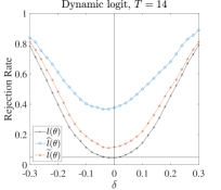
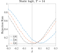
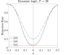
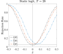
Figure 2: Size and power of LR tests for logit model with $\alpha_{i}U_{it}+\gamma_{t}V_{it}$

Notes: The plotted curves are the rejection rates of the LR tests based on $l\left(\theta\right)$ (+), $\widehat{l}\left(\theta\right)$ (o), and $\widetilde{l}\left(\theta\right)$ (*) calculated over $1000$ replications. The dynamic model is $Y_{it}=1\left(\rho_{0}Y_{it-1}+\beta_{0}X_{it}+\alpha_{i0}U_{it}+\gamma_{t0}V_{it}+\varepsilon_{it}>0\right)$ with $Y_{i0}=1\left(\beta_{0}X_{i0}+\alpha_{i0}U_{i0}+\gamma_{00}V_{i0}+\varepsilon_{i0}>0\right)$ and the static $Y_{it}=1\left(\beta_{0}X_{it}+\alpha_{i0}U_{it}+\gamma_{t0}V_{it}+\varepsilon_{it}>0\right)$, where the true value $\theta_{0}=\left(\rho_{0},\beta_{0}\right)^{\prime}=\left(0.5,1\right)^{\prime}$ for the dynamic model and $\theta_{0}=\beta_{0}=1$ for the static model respectively, $\varepsilon_{it}$ is standard-logistically distributed, $X_{it}=X_{it-1}/2+\alpha_{i0}+\gamma_{t0}+\nu_{it}$ with $\nu_{it}\sim\mathcal{N}\left(0,1/2\right)$, and $\left\{\alpha_{i0},\gamma_{t0}\right\}\sim\mathcal{N}\left(0,1/16\right)$. $U_{it}$ and $V_{it}$ are generated in the same way as $X_{it}$. $N=56$. The null is at $\theta_{0}+\delta$ where, as depicted on the horizontal axis, $\delta\in\left\{-0.3,0.28,\cdots,0.3\right\}$. The vertical line is at the true value and the horizontal at the significance level $5\%$.

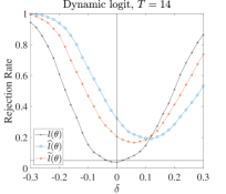
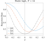
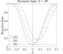
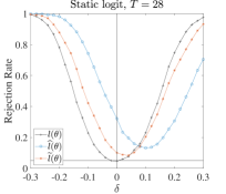
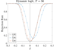
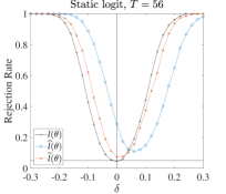
Figure 3: Size and power of LR tests for logit model with $(\lambda+\alpha_{i}+\gamma_{t})U_{it}$

Notes: The plotted curves are the rejection rates of the LR tests based on $l\left(\theta\right)$ (+), $\widehat{l}\left(\theta\right)$ (o), and $\widetilde{l}\left(\theta\right)$ (*) calculated over $1000$ replications. The dynamic model is $Y_{it}=1\left(\rho_{0}Y_{it-1}+\beta_{0}X_{it}+\left(\lambda_{0}+\alpha_{i0}+\gamma_{t0}\right)U_{it}+\varepsilon_{it}>0\right)$ with $Y_{i0}=1\left(\beta_{0}X_{i0}+\left(\lambda_{0}+\alpha_{i0}+\gamma_{00}\right)U_{i0}+\varepsilon_{i0}>0\right)$ and the static model $Y_{it}=1\left(\beta_{0}X_{it}+\left(\lambda_{0}+\alpha_{i0}+\gamma_{t0}\right)U_{it}+\varepsilon_{it}>0\right)$, where the true value $\theta_{0}=\left(\rho_{0},\beta_{0},\delta_{0}\right)^{\prime}=\left(0.5,1,1\right)^{\prime}$ for the dynamic model and $\theta_{0}=\left(\beta_{0},\delta_{0}\right)^{\prime}=\left(1,1\right)^{\prime}$ for the static model respectively, $\varepsilon_{it}$ is standard-logistically distributed, $U_{it}\sim\mathcal{N}\left(0,1/2\right)$, and $\left\{\alpha_{i0},\gamma_{t0}\right\}=0$. $N=56$. The null is at $\theta_{0}+\delta$ where, as depicted on the horizontal axis, $\delta\in\left\{-0.3,0.28,\cdots,0.3\right\}$. The vertical line is at the true value and the horizontal at the significance level $5\%$.

5 Empirical Illustration: Single Mother Labor Force Participation

In this section we apply our likelihood-based bias correction method to examining the determinants of the labor force participation (LFP) decision of single mothers. In particular, we look at the impact of the number of children on the decision of the mother to engage in paid employment.

An extensive literature in labor economics has studied the labor supply decisions of married women (Killingsworth and Heckman, 1986; Angrist and Evans, 1998; Blau and Kahn, 2007; Eckstein and Lifshitz, 2011). These studies have uncovered the impacts of a variety of economic variables, including female market wage and husband income (Mincer, 1962), education (Heath and Jayachandran, 2016), childcare costs (Connelly, 1992), the cost of home technology (Greenwood et al., 2016), and culture norms (Fernandez, 2013). Among these variables, the number of children consistently emerges as one of the most important determinants of female labor supply (Nakamura and Nakamura, 1992). This is unsurprising since women continue to bear a disproportionate share of child-rearing responsibilities (Aguero and Marks, 2008).

In contrast to the substantial body of research on the labor supply behavior of married women, the labor supply decisions of single mothers have received relatively limited attention, with only a few exceptions (Kimmel, 1998; Blundell et al., 2016). Single mothers, however, face distinctive challenges when it comes to balancing work and child-rearing responsibilities due to the absence of a second earner in the household. Moreover, their employment decisions may have a more pronounced impact on their children’s well-being compared to the decisions of married women and should thus be of great importance to economists and policymakers.

To study the labor supply decisions of single mothers, we compile a data set using waves $21-30$ of the Panel Study of Income Dynamics (PSID), which span the years of 1987 to 1996. The data set consists exclusively of single mothers, whom we define as unmarried female household heads with at least one child. Our dependent variable is labor force participation status, which we define as whether the individual has worked nonzero hours during the interview year. Our set of explanatory variables includes the number of children, which is our main treatment variable of interest, alongside age dummies. Following Dhaene and Jochmans (2015b), we restrict our sample to individuals between the age of 18 and 60 whose LFP status changed at least once during the sample period. The final sample consists of $N=98$ individuals whose labor supply status are continuously observed over a period of $T=9$ years from 1988 to 1996. See the Appendix H for more details. On average, 28 percent of these individuals switched in and out of the labor force in each year (Figure H.1$-$H.2). Table H.2 gives the summary statistics.

Let $Y_{it}\in\{0,1\}$ indicate the labor force participation status of individual $i$ in time $t$. Let $U_{it}$ denote her number of children, and let $X_{it}$ be the set of age dummies. We estimate the following two probit regressions:

$$Y_{it} =1\left\{\rho Y_{it-1}+\lambda U_{it}+\beta X_{it}+\alpha_{i}+\gamma_{t}+\varepsilon_{it}>0\right\}$$ (5.1)

$$Y_{it} =1\left\{\rho Y_{it-1}+\left(\lambda+\alpha_{i}+\gamma_{t}\right)U_{it}+\beta X_{it}+\varepsilon_{it}>0\right\},$$ (5.2)

where $1\{\cdot\}$ is an indicator function, $\varepsilon_{it}\sim\mathcal{N}\left(0,1\right)$ and $\sum_{i}\alpha_{i}=\sum_{t}\gamma_{t}=0$. In model (5.1), we focus on estimating the average treatment effect of the number of children on mother’s labor supply while controlling for unobserved heterogeneity through the inclusion of two-way fixed effects in the intercept. In model (5.2), we focus on estimating the heterogeneity in the elasticity of labor supply with respect to the number of children. This is accomplished by incorporating two-way fixed effects into the slope coefficient.

Given the “small N, small T” characteristics of our sample, direct estimation of (5.1) and (5.2) could lead to severe incidental parameter problems. Therefore, we apply our bias correction procedure to the estimation. Table 5 presents our results on Model (5.1). Let $\theta=(\rho,\lambda,\beta)$. The first two columns of the table shows the MLE ($\widehat{\theta}$) and the bias-corrected estimate ($\widetilde{\theta}$), along with standard errors computed from the Hessian matrix of their respective uncorrected and corrected profile likelihood. Looking at $\widetilde{\theta}$, we find a large and positive correlation between past and current labor force participation, indicating the existence of substantial costs for single mothers to transit in and out of the labor force. We also find that the number of children positively influences a mother’s labor supply. The presence of an additional child increases a mother’s LFP zscore by 0.239, which, on average, translates into a 9 percent higher likelihood of working. The coefficients associated with age groups are not statistically significant. Since we follow the same group of individuals over time, the effect of age is largely absorbed into $\gamma_{t}$. Comparing $\widetilde{\theta}$ with $\widehat{\theta}$, we see that the MLE under-estimates the importance of state dependence while slightly over-estimating the impact of the number of children. Bias correction leads to a 40 percent greater estimate of the former and a 6 percent lower estimate of the latter. Columns $3-8$ of Table 5 report the Wald, the LM and the LR test statistics for the null hypothesis of $\theta=0$, obtained using respectively the uncorrected and the corrected likelihood. The three tests unanimously reject $\rho=0$ and $\lambda=0$. For all parameters, bias correction results in larger statistics across all three tests. The magnitude of adjustment is particularly pronounced for lagged participation, where the test statistics more than double when computed using the corrected likelihood.

Table H.2 reports the estimation results on Model (5.2). Although not directly comparable with those of Model (5.1), these estimates reveal substantial variability in how the number of children affects a mother’s LFP. Let $\widehat{\lambda}_{it}=\widehat{\lambda}+\widehat{\alpha}_{i}+\widehat{\gamma}_{t}$ and let $\widetilde{\lambda}_{it}$ be its bias-corrected counterpart. In Figure 4a, we plot the distributions of $\widehat{\lambda}_{it}$ and $\widetilde{\lambda}_{it}$. Table H.2 reports their summary statistics. Notably, bias correction leads to a less skewed and less varied distribution, but significant heterogeneity remains after correction. In Figure 4b, we illustrate the evolution of the estimated effects over time. Looking at $\widetilde{\lambda}_{it}$, we see that in 1987, for more than half of the population, having more children is associated with a lower likelihood of labor force participation. Over time, however, there is a clear trend of increasingly positive labor supply response to having a larger number of children.

Why are single mothers on average more likely to work when they have more children? And why does this effect vary among different people over time? To delve deeper into this topic, we investigate the relationship between a mother’s labor force participation and the number of children within specific age groups. Following the approach of Dhaene and Jochmans (2015b), we categorize children into three groups: those aged 0 to 2, 3 to 5, and 6 to 17. This enables us to independently assess the impact of having more infants, preschool-age children, and school-age children on the labor supply of mothers. We proceed by re-estimating Model (5.1), with the number of children in each group as a key variable of interest.

Table 5 reports our estimation results. Looking at $\widetilde{\lambda}$, we find that the effects of having more infants or preschool children are statistically insignificant. The Wald, LM, and LR tests all fail to reject the null hypothesis of their coefficients being zero. On the other hand, the effect of having more school-age children is positive and highly statistically significant according to all three tests. This suggests that the overall positive impact of having more children on a mother’s labor supply that we observe in Model (5.1) may be primarily driven by the number of school-age children. This isn’t surprising, considering that single mothers, unlike their married counterparts who may share financial responsibilities with their spouses, often need to work to support their children’s education. These findings could also help explain the increasing trend that we observe in Model (5.2) in the heterogeneous effects of the number of children over time. Since we follow the same group of women, as their children grew up and entered school in the later years of our sample, more of them would have to enter the labor force to support their children.

Additionally, we conduct two further tests to explore specific hypotheses: (1) whether the number of infants and preschool children have the same impact on a mother’s LFP, and (2) whether the effect of the number of children on a mother’s LFP is the same regardless of children’s ages. The final two rows of Table 5 provide the test results. Both hypotheses are rejected by all three tests at the 5 percent level. This is a curious result for hypothesis (1) since neither $\lambda_{1}$ nor $\lambda_{2}$ is significant on their own. In both cases, all three test statistics become larger after bias-correction. All in all, the evidence suggests that the number of children at different stages of childhood will have different impact on their mother’s labor supply.

In summary, our analysis demonstrates the applicability of our likelihood-based bias correction method to analyze data with small $N$ and small $T$. We find that on average, an increase in the number of children corresponds to a higher likelihood of a single mother’s employment. However, these relationships exhibit heterogeneity across individuals and over time, with the impact primarily driven by the presence of school-age children, whom single mothers often need to support through education. Other findings including the importance of state dependence are consistent with literature.

[c]

Estimation results: Model (5.1)

	$\widehat{\theta}$	$\widetilde{\theta}$	$\text{Wald}_{\widehat{\theta}}$	$\text{Wald}_{\widetilde{\theta}}$	$\text{LM}_{\widehat{\theta}}$	$\text{LM}_{\widetilde{\theta}}$	$\text{LR}_{\widehat{\theta}}$	$\text{LR}_{\widetilde{\theta}}$
Lagged Participation	$0.491$	$0.690$	$18.107$	$42.440$	$18.198$	$43.326$	$17.950$	$42.409$
	$(0.115)$	$(0.106)$
# Children	$0.254$	$0.239$	$5.035$	$5.749$	$5.059$	$5.984$	$5.147$	$5.870$
	$(0.113)$	$(0.010)$
Age 30-44	$-0.267$	$-0.273$	$1.985$	$2.654$	$1.986$	$2.687$	$1.989$	$2.608$
	$(0.190)$	$(0.168)$
Age 45-60	$0.405$	$0.474$	$0.306$	$0.556$	$0.306$	$0.453$	$0.316$	$0.580$
	$(0.732)$	$(0.636)$

• Notes: Standard errors in parentheses. The Wald, the LM and the LR statistics have limiting chi-squared distributions under $H_{0}$, with critical values given by $\chi^{2}\left(1\right)_{.99}=6.635,\chi^{2}\left(1\right)_{.95}=3.841,\chi^{2}\left(1\right)_{.90}=2.706$.

[c]

Estimation results: Model (5.1) with the number of children by age groups

	$\widehat{\theta}$	$\widetilde{\theta}$	Wald${}_{\widehat{\theta}}$	Wald${}_{\widetilde{\theta}}$	LM${}_{\widehat{\theta}}$	LM${}_{\widetilde{\theta}}$	LR${}_{\widehat{\theta}}$	LR${}_{\widetilde{\theta}}$
Lagged participation ($\rho$)	$0.464$	$0.670$	$15.840$	$39.122$	$15.913$	$39.741$	$15.699$	$38.864$
	$(0.117)$	$(0.107)$
# Children 0-2 ($\lambda_{1}$)	$-0.208$	$-0.211$	$1.186$	$1.585$	$1.189$	$1.426$	$1.185$	$1.179$
	$(0.191)$	$(0.168)$
# Children 3-5 ($\lambda_{2}$)	$0.188$	$0.177$	$1.459$	$1.694$	$1.461$	$2.177$	$1.475$	$1.798$
	$(0.155)$	$(0.136)$
# Children 6-17 ($\lambda_{3}$)	$0.336$	$0.298$	$8.266$	$8.424$	$8.318$	$9.584$	$8.431$	$9.105$
	$(0.117)$	$(0.103)$
Age 30-44 ($\beta_{1}$)	$-0.289$	$-0.280$	$2.272$	$2.737$	$2.274$	$2.979$	$2.279$	$2.714$
	$(0.192)$	$(0.169)$
Age 45-60 ($\beta_{2}$)	$0.592$	$0.702$	$0.624$	$1.161$	$0.625$	$0.934$	$0.653$	$1.212$
	$(0.749)$	$(0.651)$
$\lambda_{1}=\lambda_{2}$			$4.4709$	$5.558$	$4.491$	$5.885$	$4.574$	$5.660$
$\lambda_{1}=\lambda_{2}=\lambda_{3}$			$8.911$	$10.072$	$8.999$	$10.378$	$9.190$	$10.148$

• Notes: Standard errors in parentheses. The Wald, the LM and the LR statistics have limiting chi-squared distributions under $H_{0}$, with critical values given by $\chi^{2}\left(1\right)_{.99}=6.635,\chi^{2}\left(1\right)_{.95}=3.841,\chi^{2}\left(1\right)_{.90}=2.706$ for the first 7 hypothesis tests and by $\chi^{2}\left(2\right)_{.99}=9.210,\chi^{2}\left(2\right)_{.95}=5.991,\chi^{2}\left(2\right)_{.90}=4.605$ for the last hypothesis test.

Figure 4: Distribution of elasticities of labor supply with respect to the number of children across individuals and over time based on Model (5.2) estimates.

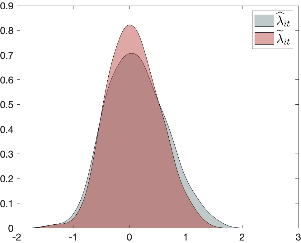
(a) Distributions of $\widehat{\lambda}_{it}$ and $\widetilde{\lambda}_{it}$

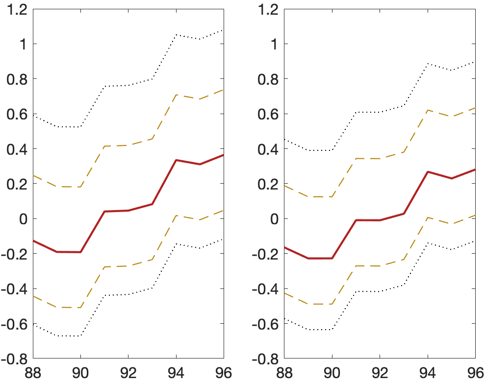
(b) Time evolution of the distributions of $\widehat{\lambda}_{it}$ (left) and $\widetilde{\lambda}_{it}$ (right). Red (solid), orange (dashed), and black (dotted) lines represent respectively the median, the (25th, 75th) percentiles, and the (10th, 90th) percentiles of the distributions in each time.

6 Conclusion

Nonlinear models with two-way fixed effects are subject to the incidental parameter problem, resulting in many test statistics failing to follow their standard asymptotic distribution under the null hypothesis. As a consequence, the sizes of these tests may depart severely from the nominal level. The purpose of this paper is to introduce an approach to bias-correct the likelihood function. The approach yields a corrected likelihood function that serves as an alternative to the original (uncorrected) likelihood for constructing hypothesis testing procedures. In particular, we prove that the three commonly used hypothesis testing procedures, the likelihood-ratio, the Lagrange-multiplier, and the Wald test, all have test statistics that follow the correct asymptotic distributions when derived from the corrected likelihood. This is not the case when they are derived from the original likelihood which is subject to the incidental parameter problem. Simulation studies and empirical analysis are further carried out to demonstrate the performance of our bias correction procedures.

The proposed approach is more general than many existing procedures. Specifically, our corrected likelihood applies to dynamic nonlinear models with two-way fixed effects and is able to revert the asymptotic distributions of test statistics from many testing procedures, whereas existing approaches mostly focus on static models or on bias-correcting the estimators, which do not benefit all testing procedures.

Appendix

AppendixAppendix

A Panel Autoregressive Model with Two-way Effects

Example A.1

Consider an autoregressive

$$Y_{it}=\rho_{0}Y_{it-1}+\alpha_{i0}+\gamma_{t0}+\varepsilon_{it}$$ (A.1)

where $0<\rho_{0}<1$ and $\varepsilon_{it}$ are i.i.d. $\mathcal{N}\left(0,1\right)$. The initial value is $Y_{i0}=0$. We assume the variance of $\varepsilon_{it}$ known so that the observation-level likelihood of $Y_{it}|Y_{it-1}$ is

$$l_{it}\left(\rho,\alpha_{i},\gamma_{t}\right)\equiv-\frac{1}{2}\log 2\pi-\frac{1}{2}\left(Y_{it}-\rho Y_{it-1}-\alpha_{i}-\gamma_{t}\right)^{2},$$

where $\left\{\alpha_{i},\gamma_{t}\right\}$ are parameters for the individual and fixed effect, respectively; and $\rho$ is the structural parameter. We impose $\sum_{i}\alpha_{i}=\sum_{t}\gamma_{t}=0$ for the identification and consider $\alpha_{i0}=\gamma_{t0}=0$ for simplicity. Let $\varepsilon_{it}\left(\rho\right)\equiv Y_{it}-\rho Y_{it-1}$. We have the MLEs

$$\widehat{\alpha}_{i}\left(\rho\right)=\frac{1}{T}\sum_{t}\varepsilon_{it}\left(\rho\right),\qquad\widehat{\gamma}_{t}\left(\rho\right)=\frac{1}{N}\sum_{i}\varepsilon_{it}\left(\rho\right);$$

and it can be shown that, seeing $\mathbb{E}\varepsilon_{it}\left(\rho\right)=\mathbb{E}Y_{it}-\rho\mathbb{E}Y_{it-1}=0$ (where the expectation is conditional on the initial value $Y_{i0}$),

$$\widehat{\alpha}_{i}\left(\rho\right)-\alpha_{i}\left(\rho\right) =O_{p}\left(T^{-1/2}\right),\qquad\alpha_{i}\left(\rho\right)=0,$$

$$\widehat{\gamma}_{t}\left(\rho\right)-\gamma_{t}\left(\rho\right) =O_{p}\left(N^{-1/2}\right),\qquad\gamma_{t}\left(\rho\right)=0.$$

Let the original and the infeasible likelihood be, respectively,

$$\widehat{l}\left(\rho\right)\equiv\frac{1}{NT}\sum_{i,t}l_{it}\left(\rho,\widehat{\alpha}_{i}\left(\rho\right),\widehat{\gamma}_{t}\left(\rho\right)\right),\qquad l\left(\rho\right)\equiv\frac{1}{NT}\sum_{i,t}l_{it}\left(\rho,\alpha_{i}\left(\rho\right),\gamma_{t}\left(\rho\right)\right).$$

$\widehat{l}\left(\rho\right)$ is subject to the IPP. In particular,

$$\sqrt{NT}\left(\mathbb{E}\widehat{l}\left(\rho\right)-\mathbb{E}l\left(\rho\right)\right)=\frac{1}{\sqrt{NT}}\sum_{i,t}\mathbb{E}\left[\varepsilon_{it}\left(\rho\right)\left(\widehat{\alpha}_{i}\left(\rho\right)+\widehat{\gamma}_{t}\left(\rho\right)\right)\right]-\frac{1}{2\sqrt{NT}}\sum_{i,t}\mathbb{E}\left(\widehat{\alpha}_{i}\left(\rho\right)+\widehat{\gamma}_{t}\left(\rho\right)\right)^{2}$$ (A.2)

and it converges to a nonzero constant as $N,T\rightarrow\infty$ with $N/T\rightarrow\kappa$. Given the cross-sectional independence, the first term on the right-hand side of (A.2),

$$\frac{1}{\sqrt{NT}}\sum_{i,t}\mathbb{E}\left[\varepsilon_{it}\left(\rho\right)\left(\widehat{\alpha}_{i}\left(\rho\right)+\widehat{\gamma}_{t}\left(\rho\right)\right)\right]$$

$$=\frac{1}{\sqrt{NT}}\frac{1}{T}\sum_{i}\sum_{t,s}\mathbb{E}\left[\varepsilon_{it}\left(\rho\right)\varepsilon_{is}\left(\rho\right)\right]+\frac{1}{\sqrt{NT}}\frac{1}{N}\sum_{i,t}\mathbb{E}\left(\varepsilon_{it}\left(\rho\right)\right)^{2},$$

converges to a nonzero constant, assuming the autocovariances of $\varepsilon_{it}\left(\rho\right)$ summable. The second term of (A.2) does so as well from the standard asymptotic theory for MLEs. Since $\sqrt{NT}(\mathbb{E}\widehat{l}\left(\rho\right)-\mathbb{E}l\left(\rho\right))$ converges to a nonzero constant, $\sqrt{NT}(\widehat{l}\left(\rho\right)-\mathbb{E}l\left(\rho\right))$ contains a bias in its asymptotic distribution.

The IPP of $\widehat{l}\left(\rho\right)$ affects its score. We have

$$\sqrt{NT}\left(\mathbb{E\triangledown}_{\rho}\widehat{l}\left(\rho\right)-\mathbb{E\triangledown}_{\rho}l\left(\rho\right)\right)$$

$$=-\frac{1}{\sqrt{NT}}\frac{1}{T}\sum_{i}\sum_{t,s}\mathbb{E}\left[Y_{it-1}\varepsilon_{is}\left(\rho\right)\right]-\frac{1}{\sqrt{NT}}\frac{1}{N}\sum_{i,t}\mathbb{E}\left[Y_{it-1}\varepsilon_{it}\left(\rho\right)\right]$$

$$+\frac{2}{\sqrt{NT}}\frac{1}{NT}\sum_{i}\sum_{t,s}\mathbb{E}\left[Y_{it-1}\varepsilon_{is}\left(\rho\right)\right].$$ (A.3)

The first two term of (A.3) converges to a nonzero constant using the same arguments above; whereas the last term converges to zero. Therefore, $\sqrt{NT}(\mathbb{E\triangledown}_{\rho}\widehat{l}\left(\rho\right)-\mathbb{E\triangledown}_{\rho}l\left(\rho\right))$ converges to a nonzero constant, inducing a bias in the asymptotic distribution of $\sqrt{NT}(\triangledown_{\rho}\widehat{l}\left(\rho\right)-\mathbb{E}\triangledown_{\rho}l\left(\rho\right))$.

B Proof of Proposition 1

B.1 Lemmas

We first introduce some Lemmas that are used during the proof. The lemma below is based on Proposition 2.5 of Fan and Yao (2003). It shows that the covariance of two measurable functions on alpha-mixing data is summable.

Lemma B.1 (summable covariances under alpha mixing)

Let Assumption 1 holds, and let $f^{\left(1\right)}\left(\theta,Z_{it}\right)$ and $f^{\left(2\right)}\left(\theta,Z_{it}\right)$ be two measurable functions bounded by $g\left(Z_{it}\right)$ uniformly in $\theta$ where $g\left(\cdot\right)$ is defined in Assumption 1. Then, as $m\rightarrow\infty$,

$$\sup_{\theta,i,t}\left|\mathbb{COV}\left(f^{\left(1\right)}\left(\theta,Z_{it}\right),f^{\left(2\right)}\left(\theta,Z_{it}\right)\right)\right| =O\left(m^{-\mu\left(1-2/\eta\right)}\right),$$ (B.1)

$${\sup_{\theta,i,t}\sum_{m=1}^{\infty}\left|\mathbb{COV}\left(f^{\left(1\right)}\left(\theta,Z_{it}\right),f^{\left(2\right)}\left(\theta,Z_{it+m}\right)\right)\right|} <\infty$$ (B.2)

where $\mu\left(1-2/\eta\right)>1$ with $\eta$ and $\mu$ defined in Assumption 1 and 1.

Proof. Applying Proposition 2.5 of Fan and Yao (2003) with $p=q=\eta$ and using the fact that $f\left(\theta,Z_{it}\right)$ is alpha mixing with the same mixing coefficient, we obtain

$$\sup_{\theta,i,t}\left|\mathbb{COV}\left(f^{\left(1\right)}\left(\theta,Z_{it}\right),f^{\left(2\right)}\left(\theta,Z_{it+m}\right)\right)\right|\leq 8\alpha(m)^{1-2/\eta}\{\mathbb{E}\sup_{i,t}g(Z_{it})^{\eta}\}^{2/\eta}.$$

Equation (B.1) follows directly from here by observing $\mathbb{E}\sup_{i,t}g(Z_{it})^{\eta}<\infty$ as in Assumption 1 and Equation (B.2) follows by observing that $m^{-\mu\left(1-2/\eta\right)}$ is a summable series in $m$.   

The next lemma states the rates of convergence of several likelihood derivatives.

Lemma B.2 (order of derivatives)

Under Assumption 1, we have that, uniformly over $\Theta$,

$$\left\|G_{\phi\phi^{\prime}}\left(\theta\right)\right\| =O\left(T^{-3/2}N^{-3/2}\right)\qquad\left\|H_{\phi\phi^{\prime}}\left(\theta\right)\right\|=O\left(T^{-1/2}N^{-1/2}\right),$$

$$\left\|\partial_{\phi}l\left(\theta\right)\right\| =O_{p}\left(T^{-3/4}N^{-3/4}\right)\qquad\left\|\partial_{\phi^{\prime}}l\left(\theta\right)\right\|=O_{p}\left(T^{-1/4}N^{-1/4}\right),$$

where $G_{\phi\phi^{\prime}}\left(\theta\right)\equiv\mathbb{E}\partial_{\phi}l\left(\theta\right)\partial_{\phi^{\prime}}l\left(\theta\right)$.

Proof. Under standard maximum likelihood asymptotic theory and Assumption 1, the last three can be shown trivially. The uniform property is a result of the assumption that the likelihood derivatives are uniformly bounded. Therefore, we focus on $\left\|G_{\phi\phi^{\prime}}\left(\theta\right)\right\|$ here. The key of showing this result is Lemma B.1. We start by observing that $G_{\phi\phi^{\prime}}\left(\theta\right)$ can be partitioned into

$$G_{\phi\phi^{\prime}}\left(\theta\right)=\begin{pmatrix}G_{\alpha\alpha^{\prime}}\left(\theta\right)&G_{\alpha\gamma^{\prime}}\left(\theta\right)\\ G_{\gamma\alpha^{\prime}}\left(\theta\right)&G_{\gamma\gamma^{\prime}}\left(\theta\right)\end{pmatrix}$$

where $G_{\gamma\alpha^{\prime}}\left(\theta\right)=\left(G_{\alpha\gamma^{\prime}}\left(\theta\right)\right)^{\prime}$ and all blocks are discussed below. All statements below are uniformly over $\theta$.

$G_{\alpha\alpha^{\prime}}\left(\theta\right)$: Under cross-sectional independence, $G_{\alpha\alpha^{\prime}}\left(\theta\right)$ is a diagonal matrix with elements

$$\mathbb{E}\left[\partial_{\alpha_{i}}l\left(\theta\right)\partial_{\alpha_{i}}l\left(\theta\right)\right] =\frac{1}{N^{2}T^{2}}\mathbb{E}\bigg{[}\sum_{t}\partial_{\alpha_{i}}l_{it}\left(\theta,\phi\left(\theta\right)\right)\bigg{]}^{2}$$

$$=\frac{1}{N^{2}T^{2}}\sum_{t}\mathbb{E}\left[\partial_{\alpha_{i}}l_{it}\left(\theta,\phi\left(\theta\right)\right)\right]^{2}$$

$$\quad+\frac{2}{N^{2}T^{2}}\sum_{t=1}^{T-1}\sum_{m=1}^{T-t}\mathbb{E}\left[\partial_{\alpha_{i}}l_{it}\left(\theta,\phi\left(\theta\right)\right)\partial_{\alpha_{i}}l_{it+m}\left(\theta,\phi\left(\theta\right)\right)\right].$$ (B.3)

By Assumption 1, the first term on the right-hand side of (B.3) is

$$\frac{1}{T}\sum_{t}\mathbb{E}[\partial_{\alpha_{i}}l_{it}\left(\theta,\phi\left(\theta\right)\right)]^{2}=O\left(1\right)$$

uniformly over $i.$ Observing $\sum_{t}\mathbb{E}\partial_{\alpha_{i}}l_{it}\left(\theta,\phi\left(\theta\right)\right)=0$, the second term on the right-hand side of (B.3) can be rewritten as

$$\sum_{t=1}^{T-1}\sum_{m=1}^{T-t}\mathbb{E}\big{[}\partial_{\alpha_{i}}l_{it}\left(\theta,\phi\left(\theta\right)\right)\partial_{\alpha_{i}}l_{it+m}\left(\theta,\phi\left(\theta\right)\right)\big{]}$$

$$= \sum_{t=1}^{T-1}\sum_{m=1}^{T-t}\mathbb{E}\big{[}\partial_{\alpha_{i}}l_{it}\left(\theta,\phi\left(\theta\right)\right)\partial_{\alpha_{i}}l_{it+m}\left(\theta,\phi\left(\theta\right)\right)\big{]}-\bigg{(}\sum_{t}\mathbb{E}\partial_{\alpha_{i}}l_{it}\left(\theta,\phi\left(\theta\right)\right)\bigg{)}\bigg{(}\sum_{t}\mathbb{E}\partial_{\alpha_{i}}l_{it}\left(\theta,\phi\left(\theta\right)\right)\bigg{)}$$

$$= \sum_{t=1}^{T-1}\sum_{m=1}^{T-t}\mathbb{E}\big{[}\partial_{\alpha_{i}}l_{it}\left(\theta,\phi\left(\theta\right)\right)\partial_{\alpha_{i}}l_{it+m}\left(\theta,\phi\left(\theta\right)\right)\big{]}-\mathbb{E}\partial_{\alpha_{i}}l_{it}\left(\theta,\phi\left(\theta\right)\right)\mathbb{E}\partial_{\alpha_{i}}l_{it+m}\left(\theta,\phi\left(\theta\right)\right)$$

$$= \sum_{t=1}^{T-1}\sum_{m=1}^{T-t}\mathbb{COV}\big{(}\partial_{\alpha_{i}}l_{it}\left(\theta,\phi\left(\theta\right)\right),\partial_{\alpha_{i}}l_{it+m}\left(\theta,\phi\left(\theta\right)\right)\big{)}$$

where, by invoking Lemma B.1, we have $\sum_{m=1}^{T-t}\mathbb{COV}\left(\partial_{\alpha_{i}}l_{it}\left(\theta,\phi\left(\theta\right)\right),\partial_{\alpha_{i}}l_{it+m}\left(\theta,\phi\left(\theta\right)\right)\right)=O\left(1\right)$ uniformly over $i$ so that

$$\frac{1}{T}\sum_{t}\sum_{m=1}^{T-t}\mathbb{E}\big{[}\partial_{\alpha_{i}}l_{it}\left(\theta,\phi\left(\theta\right)\right)\partial_{\alpha_{i}}l_{it+m}\left(\theta,\phi\left(\theta\right)\right)\big{]}=O\left(1\right).$$

The above leads to $\mathbb{E}\left[\partial_{\alpha_{i}}l\left(\theta\right)\partial_{\alpha_{i}}l\left(\theta\right)\right]=O\left(N^{-2}T^{-1}\right)$ for all $i$ so that

$$\left\|G_{\alpha\alpha^{\prime}}\left(\theta\right)\right\|=O\left(N^{-2}T^{-1}\right).$$

$G_{\gamma\gamma^{\prime}}\left(\theta\right)$: Since the data are serially correlated, $G_{\gamma\gamma^{\prime}}\left(\theta\right)$ is not a diagonal matrix. Instead, $G_{\gamma\gamma^{\prime}}\left(\theta\right)$ is a matrix with the $\left(t,t^{\prime}\right)$th element being $\mathbb{E}\partial_{\gamma_{t}}l\left(\theta\right)\partial_{\gamma_{t^{\prime}}}l\left(\theta\right)$ and the sum of absolute values of elements on the $t$th row being

$$\sum_{t^{\prime}=1}\left|\mathbb{E}\partial_{\gamma_{t}}l\left(\theta\right)\partial_{\gamma_{t^{\prime}}}l\left(\theta\right)\right| =\frac{1}{N^{2}T^{2}}\sum_{t^{\prime}}\bigg{|}\sum_{i,i^{\prime}}\mathbb{E}\partial_{\gamma_{t}}l_{it}\left(\theta,\phi\left(\theta\right)\right)\partial_{\gamma_{t^{\prime}}}l_{i^{\prime}t^{\prime}}\left(\theta,\phi\left(\theta\right)\right)\bigg{|}$$

$$\leq\frac{1}{N^{2}T^{2}}\sum_{t^{\prime}}\bigg{|}\sum_{i,i^{\prime}}\mathbb{COV}\left(\partial_{\gamma_{t}}l_{it}\left(\theta,\phi\left(\theta\right)\right),\partial_{\gamma_{t^{\prime}}}l_{i^{\prime}t^{\prime}}\left(\theta,\phi\left(\theta\right)\right)\right)\bigg{|}$$

$$+\frac{1}{N^{2}T^{2}}\sum_{t^{\prime}}\bigg{|}\sum_{i,i^{\prime}}\mathbb{E}\partial_{\gamma_{t}}l_{it}\left(\theta,\phi\left(\theta\right)\right)\mathbb{E}\partial_{\gamma_{t^{\prime}}}l_{i^{\prime}t^{\prime}}\left(\theta,\phi\left(\theta\right)\right)\bigg{|}.$$ (B.4)

The first term on the right-hand side of (B.4) rewrites,

$$\frac{1}{N^{2}T^{2}}\sum_{t^{\prime}}\bigg{|}\sum_{i,i^{\prime}}\mathbb{COV}\left(\partial_{\gamma_{t}}l_{it}\left(\theta,\phi\left(\theta\right)\right),\partial_{\gamma_{t^{\prime}}}l_{i^{\prime}t^{\prime}}\left(\theta,\phi\left(\theta\right)\right)\right)\bigg{|}$$

$$\leq \frac{1}{N^{2}T^{2}}\sum_{t^{\prime}}\bigg{|}\sum_{i\neq i^{\prime}}\mathbb{COV}\left(\partial_{\gamma_{t}}l_{it}\left(\theta,\phi\left(\theta\right)\right),\partial_{\gamma_{t^{\prime}}}l_{i^{\prime}t^{\prime}}\left(\theta,\phi\left(\theta\right)\right)\right)\bigg{|}$$

$$+\frac{1}{N^{2}T^{2}}\sum_{t^{\prime}}\bigg{|}\sum_{i}\mathbb{COV}\left(\partial_{\gamma_{t}}l_{it}\left(\theta,\phi\left(\theta\right)\right),\partial_{\gamma_{t^{\prime}}}l_{it^{\prime}}\left(\theta,\phi\left(\theta\right)\right)\right)\bigg{|}$$

where $\sum_{i\neq i^{\prime}}\mathbb{COV}\left(\partial_{\gamma_{t}}l_{it}\left(\theta,\phi\left(\theta\right)\right),\partial_{\gamma_{t^{\prime}}}l_{i^{\prime}t^{\prime}}\left(\theta,\phi\left(\theta\right)\right)\right)=0$ because of the cross-sectional independence and

$$\frac{1}{N^{2}T^{2}}\sum_{t^{\prime}}\bigg{|}\sum_{i}\mathbb{COV}\left(\partial_{\gamma_{t}}l_{it}\left(\theta,\phi\left(\theta\right)\right),\partial_{\gamma_{t^{\prime}}}l_{it^{\prime}}\left(\theta,\phi\left(\theta\right)\right)\right)\bigg{|}$$

$$\leq \frac{1}{N^{2}T^{2}}\sum_{i}\sum_{t^{\prime}}\left|\mathbb{COV}\left(\partial_{\gamma_{t}}l_{it}\left(\theta,\phi\left(\theta\right)\right),\partial_{\gamma_{t^{\prime}}}l_{it^{\prime}}\left(\theta,\phi\left(\theta\right)\right)\right)\right|$$

$$= O\left(N^{-1}T^{-2}\right),$$

because $\sum_{t^{\prime}}\left|\mathbb{COV}\left(\partial_{\gamma_{t}}l_{it}\left(\theta,\phi\left(\theta\right)\right),\partial_{\gamma_{t^{\prime}}}l_{it^{\prime}}\left(\theta,\phi\left(\theta\right)\right)\right)\right|=O\left(1\right)$ uniformly over $t$ by Lemma B.1. The second term on the right-hand side of (B.4) rewrites,

$$\frac{1}{N^{2}T^{2}}\sum_{t^{\prime}}\bigg{|}\sum_{i,i^{\prime}}\mathbb{E}\partial_{\gamma_{t}}l_{it}\left(\theta,\phi\left(\theta\right)\right)\mathbb{E}\partial_{\gamma_{t^{\prime}}}l_{i^{\prime}t^{\prime}}\left(\theta,\phi\left(\theta\right)\right)\bigg{|}$$

$$= \frac{1}{N^{2}T^{2}}\sum_{t^{\prime}}\bigg{|}\bigg{(}\sum_{i}\mathbb{E}\partial_{\gamma_{t}}l_{it}\left(\theta,\phi\left(\theta\right)\right)\bigg{)}\bigg{(}\sum_{i}\mathbb{E}\partial_{\gamma t^{\prime}}l_{it^{\prime}}\left(\theta,\phi\left(\theta\right)\right)\bigg{)}\bigg{|}$$

$$= 0$$

because $\sum_{i}\mathbb{E}\partial_{\gamma_{t}}l_{it}\left(\theta,\phi\left(\theta\right)\right)=\sum_{i}\mathbb{E}\partial_{\gamma_{t^{\prime}}}l_{it^{\prime}}\left(\theta,\phi\left(\theta\right)\right)=0$. These lead to $\sum_{t^{\prime}}\left|\mathbb{E}\partial_{\gamma_{t}}l\left(\theta\right)\partial_{\gamma_{t^{\prime}}}l\left(\theta\right)\right|=O\left(N^{-1}T^{-2}\right)$ for all $t$ so that

$$\left\|G_{\gamma\gamma^{\prime}}\left(\theta\right)\right\|=O\left(N^{-1}T^{-2}\right).$$

$G_{\alpha\gamma^{\prime}}\left(\theta\right)$: Next, $G_{\alpha\gamma^{\prime}}\left(\theta\right)$ is an $N\times T$ matrix with $\left(i,t\right)$th element being

$$\mathbb{E}[\partial_{\alpha_{i}}l\left(\theta\right)\partial_{\gamma_{t}}l\left(\theta\right)] =\frac{1}{N^{2}T^{2}}\sum_{i^{\prime},t^{\prime}}\mathbb{E}\big{[}\partial_{\alpha_{i}}l_{it^{\prime}}\left(\theta,\phi\left(\theta\right)\right)\partial_{\gamma_{t}}l_{i^{\prime}t}\left(\theta,\phi\left(\theta\right)\right)\big{]}$$

$$=\frac{1}{N^{2}T^{2}}\sum_{i^{\prime}\neq i,t^{\prime}}\mathbb{E}\big{[}\partial_{\alpha_{i}}l_{it^{\prime}}\left(\theta,\phi\left(\theta\right)\right)\partial_{\gamma_{t}}l_{i^{\prime}t}\left(\theta,\phi\left(\theta\right)\right)\big{]}$$

$$\quad+\frac{1}{N^{2}T^{2}}\sum_{t^{\prime}}\mathbb{E}\big{[}\partial_{\alpha_{i}}l_{it^{\prime}}\left(\theta,\phi\left(\theta\right)\right)\partial_{\gamma_{t}}l_{it}\left(\theta,\phi\left(\theta\right)\right)\big{]}.$$ (B.5)

Here, the first term on the right-hand side of (B.5) contains

$$\sum_{i^{\prime}\neq i,t^{\prime}}\mathbb{E}\big{[}\partial_{\alpha_{i}}l_{it^{\prime}}\left(\theta,\phi\left(\theta\right)\right)\partial_{\gamma_{t}}l_{i^{\prime}t}\left(\theta,\phi\left(\theta\right)\right)\big{]}$$

$$= \sum_{i^{\prime}\neq i,t^{\prime}}\mathbb{E}\partial_{\alpha_{i}}l_{it^{\prime}}\left(\theta,\phi\left(\theta\right)\right)\mathbb{E}\partial_{\gamma_{t}}l_{i^{\prime}t}\left(\theta,\phi\left(\theta\right)\right)$$

$$= \sum_{i^{\prime}\neq i}\sum_{t^{\prime}}\mathbb{E}\partial_{\alpha_{i}}l_{it^{\prime}}\left(\theta,\phi\left(\theta\right)\right)\mathbb{E}\partial_{\gamma_{t}}l_{i^{\prime}t}\left(\theta,\phi\left(\theta\right)\right)$$

$$= 0$$

by cross-sectional independence and by the definition of score. The second term on the right-hand side of (B.5) contains

$$\sum_{t^{\prime}}\mathbb{E}\big{[}\partial_{\alpha_{i}}l_{it^{\prime}}\left(\theta,\phi\left(\theta\right)\right)\partial_{\gamma_{t}}l_{it}\left(\theta,\phi\left(\theta\right)\right)\big{]} =\sum_{t^{\prime}}\mathbb{COV}\big{(}\partial_{\alpha_{i}}l_{it^{\prime}}\left(\theta,\phi\left(\theta\right)\right),\partial_{\gamma_{t}}l_{it}\left(\theta,\phi\left(\theta\right)\right)\big{)}$$

$$\quad+\sum_{t^{\prime}}\mathbb{E}\partial_{\alpha_{i}}l_{it^{\prime}}\left(\theta,\phi\left(\theta\right)\right)\mathbb{E}\partial_{\gamma_{t}}l_{it}\left(\theta,\phi\left(\theta\right)\right)$$

where, by Lemma B.1, $\sum_{t^{\prime}}\mathbb{COV}\left(\partial_{\alpha_{i}}l_{it^{\prime}}\left(\theta,\phi\left(\theta\right)\right),\partial_{\gamma_{t}}l_{it}\left(\theta,\phi\left(\theta\right)\right)\right)=O\left(1\right)$ and, by the definition of score, $\sum_{t^{\prime}}\mathbb{E}\partial_{\alpha_{i}}l_{it^{\prime}}\left(\theta,\phi\left(\theta\right)\right)\mathbb{E}\partial_{\gamma_{t}}l_{it}\left(\theta,\phi\left(\theta\right)\right)=0$. These lead to $\mathbb{E}\left[\partial_{\alpha_{i}}l\left(\theta\right)\partial_{\gamma_{t}}l\left(\theta\right)\right]=O\left(N^{-2}T^{-2}\right)$ for all $i,t$ so that

$$\left\|G_{\alpha\gamma^{\prime}}\left(\theta\right)\right\|=O\left(N^{-2}T^{-1}\right).$$

Since we have now identified the order of each block of $G_{\phi\phi^{\prime}}\left(\theta\right)$, it follows directly that

$$\left\|G_{\phi\phi^{\prime}}\left(\theta\right)\right\|=\max\left(\left\|\begin{pmatrix}G_{\alpha\alpha^{\prime}}\left(\theta\right)&G_{\alpha\gamma^{\prime}}\left(\theta\right)\end{pmatrix}\right\|,\left\|\begin{pmatrix}G_{\gamma\alpha^{\prime}}\left(\theta\right)&G_{\gamma\gamma^{\prime}}\left(\theta\right)\end{pmatrix}\right\|\right)$$

where

$$\left\|\begin{pmatrix}G_{\alpha\alpha^{\prime}}\left(\theta\right)&G_{\alpha\gamma^{\prime}}\left(\theta\right)\end{pmatrix}\right\|=O\left(N^{-2}T^{-1}\right),\quad\left\|\begin{pmatrix}G_{\gamma\alpha^{\prime}}\left(\theta\right)&G_{\gamma\gamma^{\prime}}\left(\theta\right)\end{pmatrix}\right\|=O\left(N^{-1}T^{-2}\right).$$

The conclusion follows from here by seeing $N/T\rightarrow\kappa$ with $0<\kappa<\infty$.   

The next lemma states that the matrix of the off-diagonal elements of $H_{\phi\phi^{\prime}}^{-1}\left(\theta\right)$ is of a smaller order than that of the diagonal elements, in terms of the $\max$-norm denoted by $\left\|\cdot\right\|_{\max}$ which is defined as $\left\|A\right\|_{\max}\equiv\max_{1\leq i\leq m,1\leq j\leq n}\left|A_{ij}\right|$ for a matrix $A$ having the $\left(i,j\right)$th element $A_{ij}$ with $i=1,\ldots,m$ and $j=1,\ldots,n$. Using this lemma, the off-diagonal elements can be dropped during the proof.

Lemma B.3 (order of inverse Hessian)

Under Assumption 1, we have

$$\left\|H_{\phi\phi^{\prime}}^{-1}\left(\theta\right)-\overline{H}_{\phi\phi^{\prime}}^{-1}\left(\theta\right)\right\|_{\max}=O\left(1\right)$$

where

$$\overline{H}_{\phi\phi^{\prime}}^{-1}\left(\theta\right)\equiv\begin{pmatrix}H_{\alpha\alpha^{\prime}}^{-1}(\theta)&0\\ 0&H_{\gamma\gamma^{\prime}}^{-1}(\theta)\end{pmatrix},$$

$$H_{\alpha\alpha^{\prime}}\left(\theta\right)\equiv\mathbb{E}\partial_{\alpha\alpha^{\prime}}l\left(\theta\right),\qquad H_{\gamma\gamma^{\prime}}\left(\theta\right)\equiv\mathbb{E}\partial_{\gamma\gamma^{\prime}}l\left(\theta\right).$$

Proof. For simplicity, we omit the argument $\theta$ during the proof. We begin by noticing

$$H_{\phi\phi^{\prime}}=\begin{pmatrix}H_{\alpha\alpha^{\prime}}&H_{\alpha\gamma^{\prime}}\\ H_{\gamma\alpha^{\prime}}&H_{\gamma\gamma^{\prime}}\end{pmatrix}$$

where $H_{\gamma\alpha^{\prime}}\equiv H_{\gamma\alpha^{\prime}}\left(\theta\right)\equiv\mathbb{E}\partial_{\gamma\alpha^{\prime}}l\left(\theta\right)$ and $H_{\alpha\gamma^{\prime}}\equiv H_{\alpha\gamma^{\prime}}\left(\theta\right)\equiv\mathbb{E}\partial_{\alpha\gamma^{\prime}}l\left(\theta\right)$. Here, $H_{\alpha\alpha^{\prime}}$ and $H_{\gamma\gamma^{\prime}}$ are diagonal matrices so that

$$\left\|H_{\alpha\alpha^{\prime}}^{-1}\right\|=O\left(N\right),\qquad\left\|H_{\gamma\gamma^{\prime}}^{-1}\right\|=O\left(T\right)$$

by the definition of $\left\|\cdot\right\|$. Similarly, $H_{\alpha\gamma^{\prime}}$ is an $N\times T$ matrix of elements with $O\left(N^{-1}T^{-1}\right)$ so that

$$\left\|H_{\alpha\gamma^{\prime}}\right\| =O\left(N^{-1}\right),\qquad\left\|H_{\gamma\alpha^{\prime}}\right\|=O\left(T^{-1}\right),$$

$$\left\|H_{\gamma\alpha^{\prime}}\right\|_{\max} =\left\|H_{\alpha\gamma^{\prime}}\right\|_{\max}=O\left(N^{-1}T^{-1}\right).$$

Denoting $H_{\phi\phi^{\prime}}^{-1}=\overline{H}_{\phi\phi^{\prime}}^{-1}+\dot{H}_{\phi\phi^{\prime}}^{-1}$, we have

$$\dot{H}_{\phi\phi^{\prime}}^{-1}\equiv\begin{pmatrix}H_{\alpha\alpha^{\prime}}^{-1}H_{\alpha\gamma^{\prime}}A^{-1}H_{\gamma\alpha^{\prime}}H_{\alpha\alpha^{\prime}}^{-1}&-H_{\alpha\alpha^{\prime}}^{-1}H_{\alpha\gamma^{\prime}}A^{-1}\\ -A^{-1}H_{\gamma\alpha^{\prime}}H_{\alpha\alpha\prime}^{-1}&H_{\gamma\gamma^{\prime}}^{-1}H_{\gamma\alpha^{\prime}}B^{-1}H_{\alpha\gamma^{\prime}}H_{\gamma\gamma^{\prime}}^{-1}\end{pmatrix}$$

by a block inversion of $H_{\phi\phi^{\prime}}$ where

$$A :=H_{\gamma\gamma^{\prime}}-H_{\gamma\alpha^{\prime}}H_{\alpha\alpha^{\prime}}^{-1}H_{\alpha\gamma^{\prime}},\quad B:=H_{\alpha\alpha^{\prime}}-H_{\alpha\gamma^{\prime}}H_{\gamma\gamma^{\prime}}^{-1}H_{\gamma\alpha^{\prime}}.$$

By Assumption 1,

$$\big{\|}H_{\alpha\alpha^{\prime}}^{-1}H_{\alpha\gamma^{\prime}}\big{\|}=\max_{i}\frac{\sum_{t}\mathbb{E}|\partial_{\alpha_{i}\gamma_{t}}l_{it}(\theta,\phi(\theta))|}{\sum_{t}-\mathbb{E}\partial_{\alpha_{i}\alpha_{i}}l_{it}(\theta,\phi(\theta))}<1,\quad\big{\|}H_{\gamma\gamma^{\prime}}^{-1}H_{\gamma\alpha^{\prime}}\big{\|}=\max_{t}\frac{\sum_{i}\mathbb{E}|\partial_{\alpha_{i}\gamma_{t}}l_{it}(\theta,\phi(\theta))|}{\sum_{i}-\mathbb{E}\partial_{\gamma_{t}\gamma_{t}}l_{it}(\theta,\phi(\theta))}<1.$$

Define

$$\tilde{A}^{-1}:= (I_{T}-{H}_{\gamma\gamma^{\prime}}^{-1}{H}_{\gamma\alpha^{\prime}}{H}_{\alpha\alpha^{\prime}}^{-1}{H}_{\alpha\gamma^{\prime}})^{-1}-I_{T}=\sum_{n=1}^{\infty}({H}_{\gamma\gamma^{\prime}}^{-1}{H}_{\gamma\alpha^{\prime}}{H}_{\alpha\alpha^{\prime}}^{-1}{H}_{\alpha\gamma^{\prime}})^{n}$$

$$\tilde{B}^{-1}:= (I_{N}-{H}_{\alpha\alpha^{\prime}}^{-1}{H}_{\alpha\gamma^{\prime}}{H}_{\gamma\gamma^{\prime}}^{-1}{H}_{\gamma\alpha^{\prime}})^{-1}-I_{N}=\sum_{n=1}^{\infty}({H}_{\alpha\alpha^{\prime}}^{-1}{H}_{\alpha\gamma^{\prime}}{H}_{\gamma\gamma^{\prime}}^{-1}{H}_{\gamma\alpha^{\prime}})^{n}$$

Then, $A^{-1}={H}_{\gamma\gamma^{\prime}}^{-1}+\tilde{A}^{-1}{H}_{\gamma\gamma^{\prime}}^{-1}$ and $B^{-1}={H}_{\alpha\alpha^{\prime}}^{-1}+\tilde{B}^{-1}{H}_{\alpha\alpha^{\prime}}^{-1}.$ Noting that $\|{H}_{\gamma\gamma^{\prime}}^{-1}{H}_{\gamma\alpha^{\prime}}{H}_{\alpha\alpha^{\prime}}^{-1}{H}_{\alpha\gamma^{\prime}}\|\leq\|{H}_{\gamma\gamma^{\prime}}^{-1}{H}_{\gamma\alpha^{\prime}}\|\|{H}_{\alpha\alpha^{\prime}}^{-1}{H}_{\alpha\gamma^{\prime}}\|<1$ by the above, we set $\|{H}_{\gamma\gamma^{\prime}}^{-1}{H}_{\gamma\alpha^{\prime}}{H}_{\alpha\alpha^{\prime}}^{-1}{H}_{\alpha\gamma^{\prime}}\|=1-d$ where $0<d<1,$ and obtain that

$$\|\tilde{A}^{-1}\|_{\max} \leq\sum_{n=0}^{\infty}(\|{H}_{\gamma\gamma^{\prime}}^{-1}{H}_{\gamma\alpha^{\prime}}{H}_{\alpha\alpha^{\prime}}^{-1}{H}_{\alpha\gamma^{\prime}}\|)^{n}\|{H}_{\gamma\gamma^{\prime}}^{-1}{H}_{\gamma\alpha^{\prime}}{H}_{\alpha\alpha^{\prime}}^{-1}{H}_{\alpha\gamma^{\prime}}\|_{\max}$$

$$\leq\sum_{n=0}^{\infty}(1-d)^{n}\cdot N\|{H}_{\gamma\gamma^{\prime}}^{-1}\|\|{H}_{\alpha\alpha^{\prime}}^{-1}\|\|{H}_{\alpha\gamma^{\prime}}\|_{\max}^{2}=O(T^{-1}).$$

Analogously, $\|\tilde{B}^{-1}\|_{\max}=O(N^{-1}).$ Thus,

$$\|A^{-1}\| =\|{H}_{\gamma\gamma^{\prime}}^{-1}\|+T\|\tilde{A}^{-1}\|_{\max}\|{H}_{\gamma\gamma^{\prime}}^{-1}\|=O(T),$$

$$\|B^{-1}\| =\|{H}_{\alpha\alpha^{\prime}}^{-1}\|+N\|\tilde{B}^{-1}\|_{\max}\|{H}_{\alpha\alpha^{\prime}}^{-1}\|=O(N).$$

Using the above and properties of $\left\|\cdot\right\|_{\max}$, it follows that

$$\left\|H_{\alpha\alpha^{\prime}}^{-1}H_{\alpha\gamma^{\prime}}A^{-1}H_{\gamma\alpha^{\prime}}H_{\alpha\alpha^{\prime}}^{-1}\right\|_{\max} \leq\left\|H_{\alpha\alpha^{\prime}}^{-1}H_{\alpha\gamma^{\prime}}A^{-1}\right\|\left\|H_{\gamma\alpha^{\prime}}H_{\alpha\alpha^{\prime}}^{-1}\right\|_{\max}$$

$$\leq\left\|H_{\alpha\alpha^{\prime}}^{-1}\right\|\left\|H_{\alpha\gamma^{\prime}}\right\|\left\|A^{-1}\right\|\left\|H_{\alpha\alpha^{\prime}}^{-1}\right\|\left\|H_{\gamma\alpha^{\prime}}\right\|_{\max}$$

$$=O\left(1\right),$$

$$\left\|H_{\alpha\alpha^{\prime}}^{-1}H_{\alpha\gamma^{\prime}}A^{-1}\right\|_{\max} =\left\|A^{-1}H_{\gamma\alpha^{\prime}}H_{\alpha\alpha\prime}^{-1}\right\|_{\max}$$

$$\leq\left\|H_{\alpha\alpha^{\prime}}^{-1}\right\|\left\|H_{\alpha\gamma^{\prime}}A^{-1}\right\|_{\max}$$

$$\leq\left\|H_{\alpha\alpha^{\prime}}^{-1}\right\|\left\|A^{-1}\right\|\left\|H_{\alpha\gamma^{\prime}}\right\|_{\max}$$

$$=O\left(1\right),$$

and

$$\left\|H_{\gamma\gamma^{\prime}}^{-1}H_{\gamma\alpha^{\prime}}B^{-1}H_{\alpha\gamma^{\prime}}H_{\gamma\gamma^{\prime}}^{-1}\right\|_{\max} \leq\|H_{\gamma\gamma^{\prime}}^{-1}\|\left\|H_{\gamma\alpha^{\prime}}\right\|\left\|B^{-1}\right\|\|H_{\gamma\gamma^{\prime}}^{-1}\|\left\|H_{\alpha\gamma^{\prime}}\right\|_{\max}$$

$$=O\left(1\right).$$

Thus, by the definition of $\left\|\cdot\right\|_{\max}$, we have $\big{\|}\dot{H}_{\phi\phi^{\prime}}^{-1}\big{\|}_{\max}=O\left(1\right)$, leading to the conclusion.   

B.2 Proof for expansion of likelihood (Equation 3.2)

The proof is based on the combination of asymptotic expansions of the likelihood and the score. In particular, since ${\partial_{\phi}}\widehat{l}\left(\theta\right)=0$, a Taylor expansion of ${\partial_{\phi}}\widehat{l}\left(\theta\right)$ around $\phi\left(\theta\right)$ would give

$$0=\partial_{\phi}l\left(\theta\right)+H_{\phi\phi^{\prime}}\left(\theta\right)\left(\widehat{\phi}\left(\theta\right)-\phi\left(\theta\right)\right)+O_{p}\left(T^{-1}\right)+O_{p}\left(N^{-1}\right),$$

leading to

$$\widehat{\phi}\left(\theta\right)-\phi\left(\theta\right)=-H_{\phi\phi^{\prime}}^{-1}\left(\theta\right)\partial_{\phi}l\left(\theta\right)+O_{p}\left(T^{-1}\right)+O_{p}\left(N^{-1}\right).$$ (B.6)

This expansion is similar to, e.g., Cox and Snell (1968) and is rather standard. Here the $O_{p}$ terms are uniform over $\theta$ because the third derivative of the likelihood is uniformly bounded and $\widehat{\phi}\left(\theta\right)$ has a finite asymptotic variance (under the standard maximum likelihood asymptotic theory). Next, Taylor-expanding $\widehat{l}\left(\theta\right)$ around $\phi\left(\theta\right)$ gives

$$\widehat{l}\left(\theta\right) =l\left(\theta\right)+\partial_{\phi^{\prime}}l\left(\theta\right)\left(\widehat{\phi}\left(\theta\right)-\phi\left(\theta\right)\right)+\frac{1}{2}\left(\widehat{\phi}\left(\theta\right)-\phi\left(\theta\right)\right)^{\prime}H_{\phi\phi^{\prime}}\left(\theta\right)\left(\widehat{\phi}\left(\theta\right)-\phi\left(\theta\right)\right)$$

$$\quad+o_{p}\big{(}N^{-1/2}T^{-1/2}\big{)},$$ (B.7)

where the remainder term is actually $o_{p}\left(N^{-1}\right)+o_{p}\left(T^{-1}\right)$ but we write $o_{p}\left(N^{-1/2}T^{-1/2}\right)$ to be consistent to what is presented in Proposition 1. In addition, by a similar argument as above, the remainder is also uniform here. Next, plugging (B.6) into (B.7),

$$l\left(\theta\right)=\widehat{l}\left(\theta\right)+\frac{1}{2}\partial_{\phi^{\prime}}l\left(\theta\right)H_{\phi\phi^{\prime}}^{-1}\left(\theta\right)\partial_{\phi}l\left(\theta\right)+o_{p}\big{(}N^{-1/2}T^{-1/2}\big{)},$$

where $\partial_{\phi^{\prime}}l\left(\theta\right)H_{\phi\phi^{\prime}}^{-1}\left(\theta\right)\partial_{\phi}l\left(\theta\right)=O_{p}\big{(}N^{-1/2}T^{-1/2}\big{)}$. Noting that the second term on the right-hand side is a quadratic form in $\partial_{\phi}l\left(\theta\right)$ and that $\mathbb{E}\partial_{\phi}l\left(\theta\right)=0$, we calculate expectations term by term to obtain

$$\mathbb{E}l\left(\theta\right) =\mathbb{E}\widehat{l}\left(\theta\right)+\frac{1}{2}\mathbb{E}\left(\partial_{\phi^{\prime}}l\left(\theta\right)H_{\phi\phi^{\prime}}^{-1}\left(\theta\right)\partial_{\phi}l\left(\theta\right)\right)+o\big{(}N^{-1/2}T^{-1/2}\big{)}$$

$$=\mathbb{E}\widehat{l}\left(\theta\right)+\frac{1}{2}\operatorname{tr}\left[H_{\phi\phi^{\prime}}^{-1}\left(\theta\right)G_{\phi\phi^{\prime}}\left(\theta\right)\right]+o\big{(}N^{-1/2}T^{-1/2}\big{)},$$

where $\operatorname{tr}\left(A\right)$ denotes the trace of a matrix $A$.

The above is an early version of Proposition 1 and it can be simplified. In particular, by Lemmas B.3 and B.2, we have

$$\left\|\left(H_{\phi\phi^{\prime}}^{-1}\left(\theta\right)-\overline{H}_{\phi\phi^{\prime}}^{-1}\left(\theta\right)\right)G_{\phi\phi^{\prime}}\left(\theta\right)\right\|_{\max} \leq\left\|H_{\phi\phi^{\prime}}^{-1}\left(\theta\right)-\overline{H}_{\phi\phi^{\prime}}^{-1}\left(\theta\right)\right\|_{\max}\left\|G_{\phi\phi^{\prime}}\left(\theta\right)\right\|$$

$$=O\big{(}T^{-3/2}N^{-3/2}\big{)}$$

and

$$\left\|\overline{H}_{\phi\phi^{\prime}}^{-1}\left(\theta\right)G_{\phi\phi^{\prime}}\left(\theta\right)\right\|_{\max}=O\left(T^{-1}N^{-1}\right),$$

so that

$$\operatorname{tr}\left[H_{\phi\phi^{\prime}}^{-1}\left(\theta\right)G_{\phi\phi^{\prime}}\left(\theta\right)\right]$$

$$= \operatorname{tr}\left[\overline{H}_{\phi\phi^{\prime}}^{-1}\left(\theta\right)G_{\phi\phi^{\prime}}\left(\theta\right)\right]+\operatorname{tr}\left[\left(H_{\phi\phi^{\prime}}^{-1}\left(\theta\right)-\overline{H}_{\phi\phi^{\prime}}^{-1}\left(\theta\right)\right)G_{\phi\phi^{\prime}}\left(\theta\right)\right]$$

$$= \operatorname{tr}\left[\overline{H}_{\phi\phi^{\prime}}^{-1}\left(\theta\right)G_{\phi\phi^{\prime}}\left(\theta\right)\right]+o\big{(}N^{-1/2}T^{-1/2}\big{)},$$

with $\operatorname{tr}\big{[}\overline{H}_{\phi\phi^{\prime}}^{-1}\left(\theta\right)G_{\phi\phi^{\prime}}\left(\theta\right)\big{]}=O\big{(}N^{-1/2}T^{-1/2}\big{)}$. Using this, we arrive at

$$\mathbb{E}l\left(\theta\right) =\mathbb{E}\widehat{l}\left(\theta\right)+\frac{1}{2}\operatorname{tr}\left[\overline{H}_{\phi\phi^{\prime}}^{-1}\left(\theta\right)G_{\phi\phi^{\prime}}\left(\theta\right)\right]+o\left(T^{-1}\right)+o\left(N^{-1}\right)$$

$$=\mathbb{E}\widehat{l}\left(\theta\right)+\frac{1}{2}\sum_{i}\frac{\mathbb{E}\partial_{\alpha_{i}}l\left(\theta\right)\partial_{\alpha_{i}}l\left(\theta\right)}{\mathbb{E}\partial_{\alpha_{i}\alpha_{i}}l\left(\theta\right)}+\frac{1}{2}\sum_{t}\frac{\mathbb{E}\partial_{\gamma_{t}}l\left(\theta\right)\partial_{\gamma_{t}}l\left(\theta\right)}{\mathbb{E}\partial_{\gamma_{t}\gamma_{t}}l\left(\theta\right)}+o\big{(}N^{-1/2}T^{-1/2}\big{)},$$ (B.8)

where the remainder is uniform over $\theta$. The numerators can be further simplified. In particular, seeing $\mathbb{E}\sum_{t}\partial_{\alpha_{i}}l_{it}\left(\theta,\phi\left(\theta\right)\right)=0$,

$$\mathbb{E}\partial_{\alpha_{i}}l\left(\theta\right)\partial_{\alpha_{i}}l\left(\theta\right) =\frac{1}{N^{2}T^{2}}\mathbb{E}\bigg{(}\sum_{t}\partial_{\alpha_{i}}l_{it}\left(\theta,\phi\left(\theta\right)\right)\bigg{)}^{2}$$

$$=\frac{1}{N^{2}T^{2}}\left[\mathbb{E}\bigg{(}\sum_{t}\partial_{\alpha_{i}}l_{it}\left(\theta,\phi\left(\theta\right)\right)\bigg{)}^{2}-\bigg{(}\sum_{t}\mathbb{E}\partial_{\alpha_{i}}l_{it}\left(\theta,\phi\left(\theta\right)\right)\bigg{)}^{2}\right]$$

$$=\frac{1}{N^{2}T^{2}}\sum_{t,t^{\prime}}\mathbb{E}\big{[}\partial_{\alpha_{i}}l_{it}\left(\theta,\phi\left(\theta\right)\right)\partial_{\alpha_{i}}l_{it^{\prime}}\left(\theta,\phi\left(\theta\right)\right)-\mathbb{E}\partial_{\alpha_{i}}l_{it}\left(\theta,\phi\left(\theta\right)\right)\mathbb{E}\partial_{\alpha_{i}}l_{it^{\prime}}\left(\theta,\phi\left(\theta\right)\right)\big{]}$$

$$=\frac{1}{N^{2}T^{2}}\sum_{t,t^{\prime}}\mathbb{E}\big{\{}\left[\partial_{\alpha_{i}}l_{it}\left(\theta,\phi\left(\theta\right)\right)-\mathbb{E}\partial_{\alpha_{i}}l_{it}\left(\theta,\phi\left(\theta\right)\right)\right]\left[\partial_{\alpha_{i}}l_{it^{\prime}}\left(\theta,\phi\left(\theta\right)\right)-\mathbb{E}\partial_{\alpha_{i}}l_{it^{\prime}}\left(\theta,\phi\left(\theta\right)\right)\right]\big{\}}$$

$$=\frac{1}{N^{2}T}\frac{1}{T}\mathbb{E}[S_{i}^{\alpha\prime}\left(\theta\right)1_{T}S_{i}^{\alpha}\left(\theta\right)].$$

Using this, the second term on the right-hand side of (B.8) becomes $\mathbb{E}b\left(\theta\right)/T$. Similarly seeing $\sum_{i}\mathbb{E}\partial_{\gamma_{t}}l_{it}\left(\theta,\phi\left(\theta\right)\right)=0$,

$$\mathbb{E}\partial_{\gamma_{t}}l\left(\theta\right)\partial_{\gamma_{t}}l\left(\theta\right) =\frac{1}{N^{2}T^{2}}\mathbb{E}\bigg{(}\sum_{i}\partial_{\gamma_{t}}l_{it}\left(\theta,\phi\left(\theta\right)\right)\bigg{)}^{2}$$

$$=\frac{1}{N^{2}T^{2}}\left[\mathbb{E}\bigg{(}\sum_{i}\partial_{\gamma_{t}}l_{it}\left(\theta,\phi\left(\theta\right)\right)\bigg{)}^{2}-\bigg{(}\mathbb{E}\sum_{i}\partial_{\gamma_{t}}l_{it}\left(\theta,\phi\left(\theta\right)\right)\bigg{)}^{2}\right]$$

$$=\frac{1}{N^{2}T^{2}}\sum_{i,i^{\prime}}\mathbb{E}\big{[}\partial_{\gamma_{t}}l_{it}\left(\theta,\phi\left(\theta\right)\right)\partial_{\gamma_{t}}l_{i^{\prime}t}\left(\theta,\phi\left(\theta\right)\right)-\mathbb{E}\partial_{\gamma_{t}}l_{it}\left(\theta,\phi\left(\theta\right)\right)\mathbb{E}\partial_{\gamma_{t}}l_{i^{\prime}t}\left(\theta,\phi\left(\theta\right)\right)\big{]}$$

$$=\frac{1}{N^{2}T^{2}}\sum_{i,i^{\prime}}\mathbb{E}\big{[}\partial_{\gamma_{t}}l_{it}\left(\theta,\phi\left(\theta\right)\right)-\mathbb{E}\partial_{\gamma_{t}}l_{it}\left(\theta,\phi\left(\theta\right)\right)\big{]}^{2}$$

$$\quad+\frac{1}{N^{2}T^{2}}\sum_{i\neq i^{\prime}}\mathbb{E}\big{[}\partial_{\gamma_{t}}l_{it}\left(\theta,\phi\left(\theta\right)\right)\partial_{\gamma_{t}}l_{i^{\prime}t}\left(\theta,\phi\left(\theta\right)\right)-\mathbb{E}\partial_{\gamma_{t}}l_{it}\left(\theta,\phi\left(\theta\right)\right)\mathbb{E}\partial_{\gamma_{t}}l_{i^{\prime}t}\left(\theta,\phi\left(\theta\right)\right)\big{]}$$

$$=\frac{1}{NT^{2}}\frac{1}{N}\mathbb{E}[S_{t}^{\gamma\prime}\left(\theta\right)S_{t}^{\gamma}\left(\theta\right)]$$

where the last equality is because of the cross-sectional independence (so that the second term on its left-hand side is ${0}$). Using this, the third term on the right hand-side of (B.8) becomes $\mathbb{E}d\left(\theta\right)/N$. Equation (3.2) follows from here.

B.3 Proof for corrected likelihood (Equation 3.3)

Given the construction of $\widetilde{l}\left(\theta\right)$, the proof of Equation 3.3 boils down to showing $\mathbb{E}\widehat{b}\left(\theta\right)-\mathbb{E}b\left(\theta\right)=o(1)$ and $\mathbb{E}\widehat{d}\left(\theta\right)-\mathbb{E}d\left(\theta\right)=o(1)$ under $N,T\rightarrow\infty$. First, uniformly over $i,$ the denominator of each ratio involves the incidental parameter Hessian evaluated at $\widehat{\phi}\left(\theta\right),$ which is consistent for its infeasible counterpart evaluated at $\phi\left(\theta\right).$ Then according to the continuous mapping theorem for convergence in probability, we only need to show that the numerators are also consistent uniformly over $i.$

For $\mathbb{E}\widehat{b}\left(\theta\right)-\mathbb{E}b\left(\theta\right)=o(1)$, we show

$$\frac{1}{T}\mathbb{E}\big{[}\widehat{S}_{i}^{\alpha\prime}\left(\theta\right)W_{\tau}\widehat{S}_{i}^{\alpha}\left(\theta\right)\big{]}-\frac{1}{T}\mathbb{E}[S_{i}^{\alpha\prime}\left(\theta\right)1_{T}S_{i}^{\alpha}\left(\theta\right)]=o(1)$$

uniformly over $i$. Recall $S_{i}^{\alpha}\left(\theta\right)\equiv\left(\partial_{\alpha_{i}}l_{i1}\left(\theta,\phi(\theta)\right)-\mathbb{E}\partial_{\alpha_{i}}l_{i1}\left(\theta,\phi(\theta)\right),\cdots,\partial_{\alpha_{i}}l_{iT}\left(\theta,\phi(\theta)\right)-\mathbb{E}\partial_{\alpha_{i}}l_{iT}\left(\theta,\phi(\theta)\right)\right)^{\prime}$. Omitting the arguments $\theta$ and $\phi(\theta)$ for simplicity,

$$\frac{1}{T}\mathbb{E}\widehat{S}_{i}^{\alpha\prime}W_{\tau}\widehat{S}_{i}^{\alpha}-\frac{1}{T}\mathbb{E}S_{i}^{\alpha\prime}1_{T}S_{i}^{\alpha}$$

$$= \frac{1}{T}\sum_{t}\mathbb{VAR}\big{(}\partial_{\alpha_{i}}\widehat{l}_{it}\big{)}-\frac{1}{T}\sum_{t}\mathbb{VAR}\left(\partial_{\alpha_{i}}l_{it}\right)$$

$$+\frac{2}{T}\sum_{m=1}^{\tau}\sum_{t=1}^{T-m}\mathbb{COV}\big{(}\partial_{\alpha_{i}}\widehat{l}_{it},\partial_{\alpha_{i}}\widehat{l}_{it+m}\big{)}-\frac{2}{T}\sum_{m=1}^{T-1}\sum_{t=1}^{T-m}\mathbb{COV}\left(\partial_{\alpha_{i}}l_{it},\partial_{\alpha_{i}}l_{it+m}\right)$$

$$= \frac{1}{T}\sum_{t}\mathbb{VAR}\big{(}\partial_{\alpha_{i}}\widehat{l}_{it}\big{)}-\frac{1}{T}\sum_{t}\mathbb{VAR}\left(\partial_{\alpha_{i}}l_{it}\right)$$

$$+\frac{2}{T}\sum_{m=1}^{\tau}\sum_{t=1}^{T-m}\mathbb{COV}\big{(}\partial_{\alpha_{i}}\widehat{l}_{it},\partial_{\alpha_{i}}\widehat{l}_{it+m}\big{)}-\frac{2}{T}\sum_{m=1}^{\tau}\sum_{t=1}^{T-m}\mathbb{COV}\left(\partial_{\alpha_{i}}l_{it},\partial_{\alpha_{i}}l_{it+m}\right)$$

$$-\frac{2}{T}\sum_{m=\tau+1}^{T-1}\sum_{t=1}^{T-m}\mathbb{COV}\left(\partial_{\alpha_{i}}l_{it},\partial_{\alpha_{i}}l_{it+m}\right).$$ (B.9)

It shall be easy to see that the first term on the right-hand side of (B.9) is $o\left(1\right)$. In addition, by invoking Lemma B.1, we also find that the second and third terms on the right-hand side of (B.9) are $o\left(1\right)$ as $\tau/T\rightarrow 0$; and, as $\tau,T\rightarrow\infty$, the last term on the right-hand side of (B.9),

$$\frac{2}{T}\sum_{m=\tau+1}^{T-1}\sum_{t=1}^{T-m}\mathbb{COV}\left(\partial_{\alpha_{i}}l_{it},\partial_{\alpha_{i}}l_{it+m}\right)$$

$$\leq 2\sum_{m=\tau+1}^{T-1}\frac{T-m}{T}\sup_{\theta,i,t}\big{|}\mathbb{COV}\left(\partial_{\alpha_{i}}l_{it},\partial_{\alpha_{i}}l_{it+m}\right)\big{|}$$

$$\leq \sum_{m=\tau+1}^{T-1}Cm^{-\mu\left(1-2/\eta\right)}=o\left(1\right)$$

for some positive constant $C<\infty$ and $\left(\mu,\eta\right)$ defined in Assumption 1 with $\mu\left(1-2/\eta\right)>1$. The above leads to $\mathbb{E}\widehat{b}\left(\theta\right)-\mathbb{E}b\left(\theta\right)=o(1)$.

For $\mathbb{E}\widehat{d}\left(\theta\right)-\mathbb{E}d\left(\theta\right)=o(1)$, an invocation of the dominated convergence theorem gives

$$\frac{1}{N}\mathbb{E}\big{[}\widehat{S}_{t}^{\gamma\prime}\left(\theta\right)\widehat{S}_{t}^{\gamma}\left(\theta\right)\big{]}-\frac{1}{N}\mathbb{E}[{S}_{t}^{\gamma\prime}\left(\theta\right){S}_{t}^{\gamma}\left(\theta\right)]=o(1),$$

which leads to $\mathbb{E}\widehat{d}\left(\theta\right)-\mathbb{E}d\left(\theta\right)=o(1)$ directly.

C Proof of Proposition 2

C.1 Lemmas

The following Lemma establishes the order of $\mathbb{E}\triangledown_{\theta\theta^{\prime}}\widehat{l}\left(\theta\right)-H_{\theta\theta^{\prime}}\left(\theta\right)$ and is needed for the proof of Proposition 2.

Lemma C.1 (order of $\theta$-Hessian)

Under Assumptions 1 to 2,

$$\sup_{\theta}\big{\|}\mathbb{E}\triangledown_{\theta\theta^{\prime}}\widehat{l}\left(\theta\right)-H_{\theta\theta^{\prime}}\left(\theta\right)\big{\|}=O\big{(}N^{-1/2}T^{-1/2}\big{)}.$$

Proof. The proof is similar to the proof of Proposition 1. First, since the dimension of $\theta$ is fixed, showing this lemma is equivalent to showing

$$\max_{q,r}\sup_{\theta\in\Theta}\big{|}\mathbb{E}\triangledown_{\theta_{q}\theta_{r}}\widehat{l}\left(\theta\right)-\mathbb{E}\triangledown_{\theta_{q}\theta_{r}}l\left(\theta\right)\big{|}=O\big{(}N^{-1/2}T^{-1/2}\big{)}$$ (C.1)

where $\theta_{q}$ and $\theta_{r}$ denotes, respectively the $q$th and $r$ th element of $\theta$. Let

$$\widehat{h} \equiv\triangledown_{\theta_{q^{\ast}}\theta_{r^{\ast}}}\widehat{l}\left(\theta^{\ast}\right),\qquad h\equiv\triangledown_{\theta_{q^{\ast}}\theta_{r^{\ast}}}l\left(\theta^{\ast}\right),$$

$$\left(q^{\ast},r^{\ast},\theta^{\ast}\right) \equiv\arg\max_{q,r,\theta}\big{|}\mathbb{E}\triangledown_{\theta_{q}\theta_{r}}\widehat{l}\left(\theta\right)-\mathbb{E}\triangledown_{\theta_{q}\theta_{r}}l\left(\theta\right)\big{|}.$$

Showing Equation (C.1) boils down to showing $\big{|}\mathbb{E}\widehat{h}-\mathbb{E}h\big{|}=O\left(N^{-1/2}T^{-1/2}\right)$.

To prove this, we consider the mean-value expansion

$$\widehat{h}=h+\partial_{\phi^{\prime}}h\left(\widehat{\phi}\left(\theta^{\ast}\right)-\phi\left(\theta^{\ast}\right)\right)+\frac{1}{2}\left(\widehat{\phi}\left(\theta^{\ast}\right)-\phi\left(\theta^{\ast}\right)\right)^{\prime}{\mathbb{E}\partial_{\phi\phi^{\prime}}\overline{h}}\left({\widehat{\phi}\left(\theta^{\ast}\right)-\phi\left(\theta^{\ast}\right)}\right)+{o_{p}\big{(}N}^{{-1/2}}{T}^{-1/2}{\big{)}}$$

where $\left\|\partial_{\phi^{\prime}}h\right\|=O_{p}\left(1\right)$, which is immediate; $\left\|\mathbb{E}\partial_{\phi\phi^{\prime}}\overline{h}\right\|=O\left(N^{-1/2}T^{-1/2}\right)$, which is the same as $\left\|H_{\phi\phi^{\prime}}\left(\theta\right)\right\|=O\left(T^{-1/2}N^{-1/2}\right)$ in Lemma B.2; and $\partial_{\phi\phi^{\prime}}\overline{h}\equiv N^{-1}T^{-1}\partial_{\phi\phi^{\prime}}\sum_{i,t}\triangledown_{\theta_{q^{\ast}}\theta_{r^{\ast}}}l_{it}\left(\theta^{\ast},\overline{\phi}\left(\theta^{\ast}\right)\right)$ with $\overline{\phi}\left(\theta^{\ast}\right)$ being a point on the segment connecting $\widehat{\phi}\left(\theta^{\ast}\right)$ and $\phi\left(\theta^{\ast}\right)$. Calculating the expectation,

$$\mathbb{E}\widehat{h}-\mathbb{E}h=\mathbb{E}\left[\partial_{\phi^{\prime}}h\left(\widehat{\phi}\left(\theta^{\ast}\right)-\phi\left(\theta^{\ast}\right)\right)\right]+\frac{1}{2}\mathbb{E}\left[\left(\widehat{\phi}\left(\theta^{\ast}\right)-\phi\left(\theta^{\ast}\right)\right)^{\prime}\mathbb{E}\partial_{\phi\phi^{\prime}}\overline{h}\left(\widehat{\phi}\left(\theta^{\ast}\right)-\phi\left(\theta^{\ast}\right)\right)\right]+o({N}^{{-1/2}}{T}^{-1/2}).$$

First, using (B.6) and noticing $\mathbb{E}\partial_{\phi}l\left(\theta^{\ast}\right)=0$, we have

$$\mathbb{E}\left[\partial_{\phi^{\prime}}h\left(\widehat{\phi}\left(\theta^{\ast}\right)-\phi\left(\theta^{\ast}\right)\right)\right] =-\mathbb{E}\left[\partial_{\phi^{\prime}}h\,H_{\phi\phi^{\prime}}^{-1}\left(\theta^{\ast}\right)\partial_{\phi}l\left(\theta^{\ast}\right)\right]+O(N^{-1/2}T^{-1/2})$$

$$=-\operatorname*{tr}\left[H_{\phi\phi^{\prime}}^{-1}\left(\theta^{\ast}\right)K_{\phi\phi^{\prime}}\left(\theta^{\ast}\right)\right]+O(N^{-1/2}T^{-1/2})$$

where $K_{\phi\phi^{\prime}}\left(\theta^{\ast}\right)=\mathbb{E}\left[\partial_{\phi}h\partial_{\phi^{\prime}}l\left(\theta^{\ast}\right)\right]$, which is the covariance matrix of $\partial_{\phi}h$ and $\partial_{\phi^{\prime}}l\left(\theta^{\ast}\right)$ since $\mathbb{E}\partial_{\phi}l\left(\theta^{\ast}\right)=0$. Now, it shall be clear that $K_{\phi\phi^{\prime}}\left(\theta^{\ast}\right)$ has a similar structure as $G_{\phi\phi^{\prime}}\left(\theta^{\ast}\right)$. Therefore, it can be verified, using the same technique as in Lemma B.2, that $\left\|K_{\phi\phi^{\prime}}\left(\theta^{\ast}\right)\right\|=O\left(T^{-3/2}N^{-3/2}\right)$. Using the same strategy in the proof of Proposition 1, we can immediately conclude that

$$\operatorname*{tr}\left[H_{\phi\phi^{\prime}}^{-1}\left(\theta^{\ast}\right)K_{\phi\phi^{\prime}}\left(\theta^{\ast}\right)\right]=O(N^{-1/2}T^{-1/2}),$$

leading to

$$\mathbb{E}\left[\partial_{\phi^{\prime}}h\left(\widehat{\phi}\left(\theta^{\ast}\right)-\phi\left(\theta^{\ast}\right)\right)\right]=O(N^{-1/2}T^{-1/2}).$$ (C.2)

Second,

$$\left|\mathbb{E}\bigg{[}\left(\widehat{\phi}\left(\theta^{\ast}\right)-\phi\left(\theta^{\ast}\right)\right)^{\prime}\mathbb{E}\partial_{\phi\phi^{\prime}}\overline{h}\left(\widehat{\phi}\left(\theta^{\ast}\right)-\phi\left(\theta^{\ast}\right)\right)\bigg{]}\right|$$

$$\leq \max\big{(}|\lambda_{\max}|,|\lambda_{\min}|\big{)}\mathbb{E}\left[\left(\widehat{\phi}\left(\theta^{\ast}\right)-\phi\left(\theta^{\ast}\right)\right)^{\prime}\left(\widehat{\phi}\left(\theta^{\ast}\right)-\phi\left(\theta^{\ast}\right)\right)\right]$$

$$\leq \left\|\mathbb{E}\partial_{\phi\phi^{\prime}}\overline{h}\right\|\mathbb{E}\left[\left(\widehat{\phi}\left(\theta^{\ast}\right)-\phi\left(\theta^{\ast}\right)\right)^{\prime}\left(\widehat{\phi}\left(\theta^{\ast}\right)-\phi\left(\theta^{\ast}\right)\right)\right]$$

where $\lambda_{\min}$ and $\lambda_{\max}$ denote the minimum and maximum eigenvalues of the symmetric matrix $\mathbb{E}\partial_{\phi\phi^{\prime}}\overline{h}$. Using $\mathbb{E}\left[\left(\widehat{\phi}\left(\theta^{\ast}\right)-\phi\left(\theta^{\ast}\right)\right)^{\prime}\left(\widehat{\phi}\left(\theta^{\ast}\right)-\phi\left(\theta^{\ast}\right)\right)\right]=O\left(1\right)$ and $\left\|\mathbb{E}\partial_{\phi\phi^{\prime}}\overline{h}\right\|=O\left(N^{-1/2}T^{-1/2}\right)$, we immediately have

$$\left|\mathbb{E}\bigg{[}\left(\widehat{\phi}\left(\theta^{\ast}\right)-\phi\left(\theta^{\ast}\right)\right)^{\prime}\mathbb{E}\partial_{\phi\phi^{\prime}}\overline{h}\left(\widehat{\phi}\left(\theta^{\ast}\right)-\phi\left(\theta^{\ast}\right)\right)\bigg{]}\right|=O\big{(}N^{-1/2}T^{-1/2}\big{)}.$$ (C.3)

Using (C.2) and (C.3), the proof is concluded.   

C.2 Proof of Proposition 2

Under our assumption of boundedness, the differentiation and expectation can be interchanged. Therefore, denoting $f\left(\theta\right)\equiv\mathbb{E}\widetilde{l}\left(\theta\right)-\mathbb{E}l\left(\theta\right)$,

$$\triangledown_{\theta}f\left(\theta\right)=\mathbb{E}\triangledown_{\theta}\widetilde{l}\left(\theta\right)-\mathbb{E}\triangledown_{\theta}l\left(\theta\right),\qquad\triangledown_{\theta\theta^{\prime}}f\left(\theta\right)=\mathbb{E}\triangledown_{\theta\theta^{\prime}}\widetilde{l}\left(\theta\right)-H_{\theta\theta^{\prime}}\left(\theta\right).$$

Next, invoking the Landau-Kolmogorov inequality, we have

$$\sup_{\theta}\left\|\triangledown_{\theta}f\left(\theta\right)\right\|\leq C\sup_{\theta}\left\|f\left(\theta\right)\right\|^{1/2}\sup_{\theta}\left\|\triangledown_{\theta\theta^{\prime}}f\left(\theta\right)\right\|^{1/2}$$

for some positive constant $C<\infty$. Here $\sup_{\theta}\left\|f\left(\theta\right)\right\|=o\left(N^{-1/2}T^{-1/2}\right)$ by (3.3) of Proposition 1; and

$$\sup_{\theta}\left\|\triangledown_{\theta\theta^{\prime}}f\left(\theta\right)\right\|$$

$$= \sup_{\theta}\bigg{\|}\mathbb{E}\triangledown_{\theta\theta^{\prime}}\widehat{l}\left(\theta\right)-H_{\theta\theta^{\prime}}\left(\theta\right)+\frac{\mathbb{E}\triangledown_{\theta\theta^{\prime}}\widehat{b}\left(\theta\right)}{T}+\frac{\mathbb{E}\triangledown_{\theta\theta^{\prime}}\widehat{d}\left(\theta\right)}{N}\bigg{\|}$$

$$\leq \sup_{\theta}\left\|\mathbb{E}\triangledown_{\theta\theta^{\prime}}\widehat{l}\left(\theta\right)-H_{\theta\theta^{\prime}}\left(\theta\right)\right\|+\frac{\sup_{\theta}\left\|\mathbb{E}\triangledown_{\theta\theta^{\prime}}\widehat{b}\left(\theta\right)\right\|}{T}+\frac{\sup_{\theta}\left\|\mathbb{E}\triangledown_{\theta\theta^{\prime}}\widehat{d}\left(\theta\right)\right\|}{N}$$

$$=O\big{(}N^{-1/2}T^{-1/2}\big{)}$$

where the final order is because of Lemma C.1 together with the fact that $\sup_{\theta}\big{\|}\mathbb{E}\triangledown_{\theta\theta^{\prime}}\widehat{b}\left(\theta\right)\big{\|}=O\left(1\right)$ and $\sup_{\theta}\big{\|}\mathbb{E}\triangledown_{\theta\theta^{\prime}}\widehat{d}\left(\theta\right)\big{\|}=O\left(1\right)$ which can be verified by a similar argument as the proof of (3.3) of Proposition 1. The conclusion follows naturally from here.

D Proof of Theorem 1

D.1 Lemmas

The following Lemma states that $\triangledown_{\theta}\widetilde{l}\left(\theta\right)-\triangledown_{\theta}l\left(\theta\right)=o_{p}(N^{-1/2}T^{-1/2})$ uniformly. This result is used during the proofs of Lemma D.2 and Theorem 1. Note, this lemma follows from Proposition 2 quite easily and does not depend on Assumption 3 at all.

Lemma D.1 (asymptotic equivalence of corrected score)

Under Assumptions 1 to 2, we have

$$\sup_{\theta\in\Theta}\left\|\triangledown_{\theta}\widetilde{l}\left(\theta\right)-\triangledown_{\theta}l\left(\theta\right)\right\|=o_{p}(N^{-1/2}T^{-1/2}).$$

Proof. Using Proposition 1, we have

$$\sqrt{NT}\left[\triangledown_{\theta}\widetilde{l}\left(\theta\right)-\mathbb{E}\triangledown_{\theta}\widetilde{l}\left(\theta\right)\right] =\frac{1}{\sqrt{NT}}\sum_{i,t}\left(\triangledown_{\theta}l_{it}(\theta,\widehat{\phi}\left(\theta\right))-\mathbb{E}\triangledown_{\theta}l_{it}(\theta,\widehat{\phi}\left(\theta\right))\right)$$

$$\quad+{\frac{\sqrt{NT}}{T}}\frac{1}{2N}\sum_{i}\left({\triangledown_{\theta}\widehat{b}}_{{i}}{\left(\theta\right)-\mathbb{E}\triangledown_{\theta}\widehat{b}}_{{i}}{\left(\theta\right)}\right)+{\frac{\sqrt{NT}}{N}}\frac{1}{2T}\sum_{t}\left({\triangledown_{\theta}\widehat{d}}_{{t}}{\left(\theta\right)-\mathbb{E}\triangledown_{\theta}\widehat{d}}_{{t}}{\left(\theta\right)}\right)$$

where ${\widehat{b}}_{{i}}{\left(\theta\right)\equiv}1/T\mathbb{[}\widehat{S}_{i}^{\alpha\prime}\left(\theta\right)W_{\tau}\widehat{S}_{i}^{\alpha}\left(\theta\right)]/\widehat{h}_{i}^{\alpha}\left(\theta\right)$ and ${\widehat{d}}_{{t}}{\left(\theta\right)\equiv}1/N[\widehat{S}_{t}^{\gamma\prime}\left(\theta\right)\widehat{S}_{t}^{\gamma}\left(\theta\right)]/\widehat{h}_{t}^{\gamma}\left(\theta\right)$. Here, by similar arguments as in the proof of (3.3) in Proposition 1, $\mathbb{E}\triangledown_{\theta}\widehat{b}_{i}\left(\theta\right)=O(1)\quad$and$\quad\mathbb{E}\triangledown_{\theta}\widehat{d}_{t}\left(\theta\right)=O(1)$ uniformly over $i$ and $t$ respectively. Therefore, by the law of large numbers,

$$\frac{1}{N}\sum_{i}\left({\triangledown_{\theta}\widehat{b}}_{{i}}{\left(\theta\right)-\mathbb{E}\triangledown_{\theta}\widehat{b}}_{{i}}{\left(\theta\right)}\right)=o_{p}\left(1\right),\qquad\frac{1}{T}\sum_{t}\left({\triangledown_{\theta}\widehat{d}}_{{t}}{\left(\theta\right)-\mathbb{E}\triangledown_{\theta}\widehat{d}}_{{t}}{\left(\theta\right)}\right)=o_{p}\left(1\right),$$

leading to

$$\sqrt{NT}\left(\triangledown_{\theta}\widetilde{l}\left(\theta\right)-\mathbb{E}\triangledown_{\theta}\widetilde{l}\left(\theta\right)\right) =\frac{1}{\sqrt{NT}}\sum_{i,t}\left(\triangledown_{\theta}l_{it}(\theta,\widehat{\phi}\left(\theta\right))-\mathbb{E}\triangledown_{\theta}l_{it}(\theta,\widehat{\phi}\left(\theta\right))\right)+o_{p}\left(1\right)$$

$$=\frac{1}{\sqrt{NT}}\sum_{i,t}\big{(}\triangledown_{\theta}l_{it}(\theta,\phi\left(\theta\right))-\mathbb{E}\triangledown_{\theta}l_{it}(\theta,\phi\left(\theta\right))\big{)}+o_{p}\left(1\right)$$

$$=\sqrt{NT}\big{(}\triangledown_{\theta}l\left(\theta\right)-\mathbb{E}\triangledown_{\theta}l\left(\theta\right)\big{)}+o_{p}\left(1\right)$$ (D.1)

where the last equality can be shown by a uniform linear approximation near $\phi\left(\theta\right)$. Now,

$$\sup_{\theta\in\Theta}\left\|\triangledown_{\theta}\widetilde{l}\left(\theta\right)-\triangledown_{\theta}l\left(\theta\right)\right\|$$

$$\leq \sup_{\theta\in\Theta}\left\|\left(\triangledown_{\theta}\widetilde{l}\left(\theta\right)-\mathbb{E}\triangledown_{\theta}\widetilde{l}\left(\theta\right)\right)-\left(\triangledown_{\theta}l\left(\theta\right)-\mathbb{E}\triangledown_{\theta}l\left(\theta\right)\right)\right\|$$

$$+\sup_{\theta\in\Theta}\left\|\mathbb{E}\triangledown_{\theta}\widetilde{l}\left(\theta\right)-\mathbb{E}\triangledown_{\theta}l\left(\theta\right)\right\|.$$

Using Proposition 2 and seeing that the remainder term of (D.1) is uniform in $\theta$, the proof concludes here.   

The following lemma establishes the consistency and asymptotic normality of $\widetilde{\theta}$.

Lemma D.2 (asymptotic properties of $\widetilde{\theta}$)

Under Assumptions 1 to 2 and Condition 3 of Assumption 3,

$$\big{\|}\widetilde{\theta}-\theta_{0}\big{\|}\rightarrow_{p}0,\qquad\sqrt{NT}\big{(}\widetilde{\theta}-\theta_{0}\big{)}\rightarrow_{d}\mathcal{N}\left(0,\Sigma\right)$$

where

$$\Sigma \equiv\lim_{N,T\rightarrow\infty}[H_{\theta\theta^{\prime}}(\theta_{0})]^{-1}\Omega(\theta_{0})[H_{\theta\theta^{\prime}}(\theta_{0})]^{-1},$$

$$\Omega(\theta_{0}) \equiv\lim_{N,T\rightarrow\infty}\frac{1}{NT}\sum_{i=1}^{N}\sum_{t=1}^{T}\sum_{s=1}^{T}\mathbb{E}\big{[}\triangledown_{\theta}l_{it}(\theta_{0},\phi\left(\theta_{0}\right))\triangledown_{\theta^{\prime}}l_{is}(\theta_{0},\phi\left(\theta_{0}\right))\big{]}.$$

Proof. We first show the consistency of $\widetilde{\theta}$. The key point here is that $\widetilde{l}\left(\theta\right)$ converges uniformly to $\mathbb{E}l\left(\theta\right)$ since $\widehat{l}\left(\theta\right)$ does and the correction terms $b\left(\theta\right)$ and $d\left(\theta\right)$ are uniformly bounded. In particular, $\widetilde{l}\left(\theta\right)-\mathbb{E}l\left(\theta\right)=o_{p}\left(1\right)$ uniformly in $\theta\in\Theta$, so that

$$\lim_{N,T\rightarrow\infty}\Pr\left[\big{|}\widetilde{l}(\widetilde{\theta})-\mathbb{E}l(\widetilde{\theta})\big{|}<\epsilon/3\right] =1,$$

$$\lim_{N,T\rightarrow\infty}\Pr\left[\big{|}\widetilde{l}(\theta_{0})-\mathbb{E}l(\theta_{0})\big{|}<\epsilon/3\right] =1$$

for every $\epsilon>0$. Also, since $\widetilde{\theta}$ is the unique maximizer of $\widetilde{l}(\theta)$, $\widetilde{l}(\widetilde{\theta})>\widetilde{l}(\theta_{0})-{\epsilon}/3$ for $\epsilon$ small. Combining these three,

$$\mathbb{E}l(\widetilde{\theta})-\mathbb{E}l(\theta_{0})$$

$$> \big{(}\mathbb{E}l(\widetilde{\theta})-\widetilde{l}(\widetilde{\theta})\big{)}+\big{(}\widetilde{l}(\widetilde{\theta})-\widetilde{l}(\theta_{0})\big{)}+\big{(}\widetilde{l}(\widetilde{\theta}_{0})-\mathbb{E}l(\theta_{0})\big{)}$$

$$> -\epsilon,$$ (D.2)

with probability approaching ${1}$. Notice that $\mathbb{E}l(\theta)$ is continuous in $\theta$ since $l(\theta)$ is so. Next, denote

$$\Theta_{\epsilon}\equiv\left\{\theta\in\Theta:\left\|\theta-\theta_{0}\right\|<\epsilon\right\}$$

for given $\epsilon>0$. Here, since $\Theta$ is compact and $\Theta_{\epsilon}$ is open, $\Theta_{\epsilon}^{c}\equiv\Theta\backslash\Theta_{\epsilon}$ is compact. This, together with the continuity of $\mathbb{E}l(\theta)$, indicates that there exists a $\theta^{\ast}\in\Theta_{\epsilon}^{c}$ such that $\mathbb{E}l(\theta^{\ast})={\max}_{\theta\in\Theta_{\epsilon}^{c}}\mathbb{E}l(\theta)$. On the other hand, $\theta_{0}$ is the global maximizer of $\mathbb{E}l(\theta)$ over $\Theta$ by assumption, we may conclude that

$$\mathbb{E}l(\theta_{0})>\mathbb{E}l(\theta^{\ast}),$$

For every small enough $\epsilon<\mathbb{E}l(\theta_{0})-\mathbb{E}l(\theta^{\ast})$, we have $\mathbb{E}l(\theta_{0})-\mathbb{E}l(\widetilde{\theta})<\epsilon<{\mathbb{E}l(\theta_{0})-\mathbb{E}l(\theta^{\ast})}$ with probability approaching ${1}$ by (D.2), so that

$$\mathbb{E}l(\widetilde{\theta})>\mathbb{E}l(\theta^{\ast})$$

with probability approaching $1$. Now, since $\theta^{\ast}$ is the maximizer of $\mathbb{E}l(\theta)$ over $\Theta$${}_{\epsilon}^{c}$, this implies $\widetilde{\theta}\notin\Theta$${}_{\epsilon}^{c}$, and thus

$$\big{\|}\widetilde{\theta}-\theta_{0}\big{\|}\rightarrow_{p}0$$

as $N,T\rightarrow\infty$.

For the asymptotic normality, standard technique applies. Consider a mean value expansion of $\sqrt{NT}\triangledown_{\theta}\widetilde{l}(\widetilde{\theta})=0$ around $\theta_{0}$, i.e.,

$$0=\sqrt{NT}\triangledown_{\theta}\widetilde{l}(\theta_{0})+\triangledown_{\theta\theta^{\prime}}\widetilde{l}(\overline{\theta})\sqrt{NT}(\widetilde{\theta}-\theta_{0})$$

where $\overline{\theta}$ is a point on the segment connecting $\widetilde{\theta}$ and $\theta_{0}$. By Lemma D.1, we can immediately see

$$\sqrt{NT}(\widetilde{\theta}-\theta_{0}) =-[\triangledown_{\theta\theta^{\prime}}\widetilde{l}(\overline{\theta})]^{-1}\sqrt{NT}\triangledown_{\theta}\widetilde{l}(\theta_{0})$$

$$=-[\triangledown_{\theta\theta^{\prime}}\widetilde{l}(\overline{\theta})]^{-1}\sqrt{NT}\triangledown_{\theta}{l}(\theta_{0})+o_{p}(1)$$

$$=-[H_{\theta\theta^{\prime}}(\theta_{0})]^{-1}\sqrt{NT}\triangledown_{\theta}{l}(\theta_{0})+o_{p}(1),$$ (D.3)

where the last equality is because of $\triangledown_{\theta\theta^{\prime}}\widetilde{l}(\overline{\theta})-H_{\theta\theta^{\prime}}(\theta_{0})=o_{p}(1)$ with invertible $H_{\theta\theta^{\prime}}(\theta_{0})$. From here, the conclusion follows that

$$\sqrt{NT}\big{(}\widetilde{\theta}-\theta_{0}\big{)}\rightarrow_{d}\mathcal{N}\left(0,\Sigma\right)$$

with the asymptotic covariance matrix

$$\Sigma=\lim_{N,T\rightarrow\infty}[H_{\theta\theta^{\prime}}(\theta_{0})]^{-1}\Omega(\theta_{0})[H_{\theta\theta^{\prime}}(\theta_{0})]^{-1}$$

where

$$\Omega(\theta_{0}) =\lim_{N,T\rightarrow\infty}\frac{1}{NT}\sum_{i=1}^{N}\sum_{j=1}^{N}\sum_{t=1}^{T}\sum_{s=1}^{T}\mathbb{E}\big{[}\triangledown_{\theta}l_{it}(\theta_{0},\phi\left(\theta_{0}\right))\triangledown_{\theta^{\prime}}l_{js}(\theta_{0},\phi\left(\theta_{0}\right))\big{]}$$

$$=\lim_{N,T\rightarrow\infty}\frac{1}{NT}\sum_{i=1}^{N}\sum_{t=1}^{T}\sum_{s=1}^{T}\mathbb{E}\big{[}\triangledown_{\theta}l_{it}(\theta_{0},\phi\left(\theta_{0}\right))\triangledown_{\theta^{\prime}}l_{is}(\theta_{0},\phi\left(\theta_{0}\right))\big{]}$$

provided that the cross-section is independent. The proof concludes here.   

The next lemma presents the limiting random variable of $\sqrt{NT}\big{(}\widetilde{\theta}_{R}-\widetilde{\theta}\big{)}$. This result is used to establish the asymptotic distributions of $\widetilde{\xi}_{LR}$ and $\widetilde{\xi}_{LM}$ which are written in terms of $\sqrt{NT}\big{(}\widetilde{\theta}_{R}-\widetilde{\theta}\big{)}$.

Lemma D.3 (Asymptotic representation about $\widetilde{\theta}_{R}$)

Under Assumptions 1 to 3 and $H_{0}:R\left(\theta_{0}\right)=0$,

$$\sqrt{NT}\left(\widetilde{\theta}_{R}-\widetilde{\theta}\right)=\Xi\left(\theta_{0}\right)\sqrt{NT}\triangledown_{\theta}l(\theta_{0})+o_{p}\left(1\right)$$

where, as in the main text,

$$\Xi\left(\theta_{0}\right)\equiv\left[H_{\theta\theta^{\prime}}(\theta_{0})\right]^{-1}\left[J(\theta_{0})\right]^{\prime}\left(J(\theta_{0})\left[H_{\theta\theta^{\prime}}(\theta_{0})\right]^{-1}\left[J(\theta_{0})\right]^{\prime}\right)^{-1}J(\theta_{0})\left[H_{\theta\theta^{\prime}}(\theta_{0})\right]^{-1}.$$

Proof. We consider the constrained maximization problem

$$\left\{\widetilde{\theta}_{R},\widetilde{b}\right\}\equiv\arg\max_{\theta,b}\widetilde{l}(\theta)+b^{\prime}R\left(\theta\right)$$

where $b$ is the Lagrangian multiplier. The constrained maximization problem has the first-order conditions

$$\sqrt{NT}\triangledown_{\theta}\widetilde{l}(\widetilde{\theta}_{R})+\left[J(\widetilde{\theta}_{R})\right]^{\prime}\sqrt{NT}\widetilde{b} =0,$$ (D.4)

$$\sqrt{NT}R(\widetilde{\theta}_{R}) =0.$$ (D.5)

Because $\widetilde{\theta}_{R}$ is an asymptotically normal estimator under the null hypothesis, $\sqrt{NT}\big{(}\widetilde{\theta}_{R}-\theta_{0}\big{)}=O_{p}\left(1\right)$ following from a similar proof as in Lemma D.2. Moreover, $\sqrt{NT}\widetilde{b}=O_{p}(1)$ as implied by (D.4) seeing $\sqrt{NT}\triangledown_{\theta}\widetilde{l}(\theta_{0})=O_{p}(1)$ and $J(\theta_{0})$ is of full row rank. Now, We mean-value expand $\sqrt{NT}\triangledown_{\theta}\widetilde{l}(\widetilde{\theta}_{R})$ around $\theta_{0}$ to obtain

$$\sqrt{NT}\triangledown_{\theta}\widetilde{l}(\widetilde{\theta}_{R}) =\sqrt{NT}\triangledown_{\theta}\widetilde{l}(\theta_{0})+\triangledown_{\theta\theta^{\prime}}\widetilde{l}(\overline{\theta})\sqrt{NT}\big{(}\widetilde{\theta}_{R}-\theta_{0}\big{)}$$

$$=\sqrt{NT}\triangledown_{\theta}\widetilde{l}(\theta_{0})+H_{\theta\theta^{\prime}}(\theta_{0})\sqrt{NT}\big{(}\widetilde{\theta}_{R}-\theta_{0}\big{)}+o_{p}(1).$$ (D.6)

where $\overline{\theta}$ is a point on the segment connecting $\widetilde{\theta}_{R}$ and $\theta_{0}$; and the last equality is because of $\triangledown_{\theta\theta^{\prime}}\widetilde{l}(\overline{\theta})\rightarrow_{p}H_{\theta\theta^{\prime}}(\theta_{0})$. Seeing $J(\widetilde{\theta}_{R})\rightarrow_{p}J(\theta_{0})$ and $\sqrt{NT}\widetilde{b}=O_{p}(1)$, A combination of (D.4) and (D.6) yields

$$H_{\theta\theta^{\prime}}(\theta_{0})\sqrt{NT}(\widetilde{\theta}_{R}-\theta_{0})+\left[J(\theta_{0})\right]^{\prime}\sqrt{NT}\widetilde{b}=-\sqrt{NT}\triangledown_{\theta}\widetilde{l}(\theta_{0})+o_{p}(1).$$ (D.7)

Similarly for Equation (D.5),

$$0 =\sqrt{NT}R(\widetilde{\theta}_{R})$$

$$=\sqrt{NT}R(\theta_{0})+J(\theta_{0})\sqrt{NT}\big{(}\widetilde{\theta}_{R}-\theta_{0}\big{)}+o_{p}(1)$$

$$=J(\theta_{0})\sqrt{NT}\big{(}\widetilde{\theta}_{R}-\theta_{0}\big{)}+o_{p}(1).$$ (D.8)

where the last equality is because of $\sqrt{NT}R(\theta_{0})=0$. Now, Equations (D.7) and (D.8) represent the system of linear equations

$$\begin{pmatrix}H_{\theta\theta^{\prime}}(\theta_{0})&\left[J(\theta_{0})\right]^{\prime}\\ J(\theta_{0})&0\end{pmatrix}\begin{pmatrix}\sqrt{NT}(\widetilde{\theta}_{R}-\theta_{0})\\ \sqrt{NT}\widetilde{b}\end{pmatrix}=\begin{pmatrix}-\sqrt{NT}\triangledown_{\theta}\widetilde{l}(\theta_{0})\\ 0\end{pmatrix}+o_{p}(1)$$ (D.9)

which has the solution

$$\sqrt{NT}\big{(}\widetilde{\theta}_{R}-\theta_{0}\big{)}=-\left(\left[H_{\theta\theta^{\prime}}(\theta_{0})\right]^{-1}-\Xi\left(\theta_{0}\right)\right)\sqrt{NT}\triangledown_{\theta}\widetilde{l}(\theta_{0})+o_{p}\left(1\right).$$

Invoking Lemma D.1,

$$\sqrt{NT}\big{(}\widetilde{\theta}_{R}-\theta_{0}\big{)}=-\left(\left[H_{\theta\theta^{\prime}}(\theta_{0})\right]^{-1}-\Xi\left(\theta_{0}\right)\right)\sqrt{NT}\triangledown_{\theta}l(\theta_{0})+o_{p}\left(1\right).$$ (D.10)

The conclusion follows by subtracting (D.3) in Lemma D.2 from (D.10).   

D.2 Proof of Theorem 1

Since $\widetilde{\xi}_{LR}$, $\widetilde{\xi}_{LM}$, and $\widetilde{\xi}_{Wald}$ are constructed in the context of maximum likelihood, we make use of the information matrix equality here; i.e., let $\Sigma$ in Lemma D.2 reduce to $\Sigma=-\lim_{N,T\rightarrow\infty}\left[H_{\theta\theta^{\prime}}(\theta_{0})\right]^{-1}$. Our proof strategy is to first show

$$\widetilde{\xi}_{LR}=\widetilde{\xi}+o_{p}(1),\qquad\widetilde{\xi}_{LM}=\widetilde{\xi}+o_{p}(1),\qquad\widetilde{\xi}_{Wald}=\widetilde{\xi}+o_{p}(1)$$

where

$$\widetilde{\xi}\equiv-\sqrt{NT}\triangledown_{\theta^{\prime}}l(\theta_{0})\left[H_{\theta\theta^{\prime}}(\theta_{0})\right]^{-1}\left[J(\theta_{0})\right]^{\prime}\left(J(\theta_{0})\left[H_{\theta\theta^{\prime}}(\theta_{0})\right]^{-1}\left[J(\theta_{0})\right]^{\prime}\right)^{-1}J(\theta_{0})\left[H_{\theta\theta^{\prime}}(\theta_{0})\right]^{-1}\sqrt{NT}\triangledown_{\theta}l(\theta_{0}).$$

Then we show $\widetilde{\xi}\rightarrow_{d}\chi^{2}\left(r\right)$. We take the consistency of $\widetilde{\theta}_{R}$ given, since the proof is analogous to that of $\widetilde{\theta}$ under $H_{0}$.

We start from showing $\widetilde{\xi}_{LR}=\widetilde{\xi}+o_{p}(1)$. In particular, a mean value expansion of $\widetilde{l}(\widetilde{\theta}_{R})$ around $\widetilde{\theta}$ gives

$$\widetilde{l}(\widetilde{\theta}_{R})=\widetilde{l}(\widetilde{\theta})+\triangledown_{\theta^{\prime}}\widetilde{l}(\widetilde{\theta})\left(\widetilde{\theta}_{R}-\widetilde{\theta}\right)+\frac{1}{2}\left(\widetilde{\theta}_{R}-\widetilde{\theta}\right)^{\prime}\triangledown_{\theta\theta^{\prime}}\widetilde{l}(\dot{\theta})\left(\widetilde{\theta}_{R}-\widetilde{\theta}\right)$$

where $\dot{\theta}$ is between $\widetilde{\theta}_{R}$ and $\widetilde{\theta}$. Since $\triangledown_{\theta^{\prime}}\widetilde{l}(\widetilde{\theta})=0$ and $\triangledown_{\theta\theta^{\prime}}\widetilde{l}(\dot{\theta})-H_{\theta\theta^{\prime}}(\theta_{0})=o_{p}(1)$, we immediately have

$$\widetilde{\xi}_{LR} =-NT\left(\widetilde{\theta}_{R}-\widetilde{\theta}\right)^{\prime}\triangledown_{\theta\theta^{\prime}}\widetilde{l}(\dot{\theta})\left(\widetilde{\theta}_{R}-\widetilde{\theta}\right)$$

$$=\widetilde{\xi}+o_{p}\left(1\right)$$

where the last equality is by invoking Lemma D.3 seeing that $\triangledown_{\theta\theta^{\prime}}\widetilde{l}(\dot{\theta})$ is consistent for $H_{\theta\theta^{\prime}}(\theta_{0})$. Similarly for $\widetilde{\xi}_{LM}$, we have

$$\sqrt{NT}\triangledown_{\theta}\widetilde{l}(\widetilde{\theta}_{R}) =\sqrt{NT}\triangledown_{\theta}\widetilde{l}(\widetilde{\theta})+\triangledown_{\theta\theta^{\prime}}\widetilde{l}(\dot{\theta})\sqrt{NT}\left(\widetilde{\theta}_{R}-\widetilde{\theta}\right)$$

$$=H_{\theta\theta^{\prime}}(\theta_{0})\sqrt{NT}\left(\widetilde{\theta}_{R}-\widetilde{\theta}\right)+o_{p}\left(1\right),$$

where $\dot{\theta}$ is between $\widetilde{\theta}_{R}$ and $\widetilde{\theta}$ (not necessarily the same as $\dot{\theta}$ for $\widetilde{\xi}_{LR}$). It follows from the same argument that

$$\widetilde{\xi}_{LM} =-\sqrt{NT}\left(\widetilde{\theta}_{R}-\widetilde{\theta}\right)^{\prime}H_{\theta\theta^{\prime}}(\theta_{0})\left[\triangledown_{\theta\theta^{\prime}}\widetilde{l}(\widetilde{\theta}_{R})\right]^{-1}H_{\theta\theta^{\prime}}(\theta_{0})\sqrt{NT}\left(\widetilde{\theta}_{R}-\widetilde{\theta}\right)+o_{p}\left(1\right)$$

$$=\widetilde{\xi}+o_{p}\left(1\right).$$

For $\widetilde{\xi}_{Wald}$, a mean-value expansion of $R(\widetilde{\theta})$ gives

$$\sqrt{NT}R(\widetilde{\theta})=\sqrt{NT}R(\widetilde{\theta}_{R})+J(\dot{\theta})\sqrt{NT}\left(\widetilde{\theta}-\widetilde{\theta}_{R}\right)$$

where $\dot{\theta}$ is between $\widetilde{\theta}_{R}$ and $\widetilde{\theta}$. By Lemma D.3, seeing that $\dot{\theta}$ is consistent for $\theta_{0}$ and that $R(\widetilde{\theta}_{R})=0$ by definition, we have

$$\widetilde{\xi}_{Wald} =-\sqrt{NT}\left(\widetilde{\theta}-\widetilde{\theta}_{R}\right)^{\prime}\left[J(\dddot{\theta})\right]^{\prime}\left[J(\widetilde{\theta})[\triangledown_{\theta\theta^{\prime}}\widetilde{l}(\widetilde{\theta})]^{-1}J(\widetilde{\theta})^{\prime}\right]^{-1}J(\dot{\theta})\sqrt{NT}\left(\widetilde{\theta}-\widetilde{\theta}_{R}\right)$$

$$=\widetilde{\xi}+o_{p}\left(1\right).$$

Next, for $\widetilde{\xi}\rightarrow_{d}\chi^{2}\left(r\right)$, we have $\sqrt{NT}\triangledown_{\theta}l(\theta_{0})\rightarrow_{d}\mathcal{N}\left(0,-\lim_{N,T\rightarrow\infty}H_{\theta\theta^{\prime}}(\theta_{0})\right)$ so that the delta method gives

$$J(\theta_{0})\left[H_{\theta\theta^{\prime}}(\theta_{0})\right]^{-1}\sqrt{NT}\triangledown_{\theta}l(\theta_{0})\rightarrow_{d}\mathcal{N}\left(0,-J(\theta_{0})\lim_{N,T\rightarrow\infty}\left[H_{\theta\theta^{\prime}}(\theta_{0})\right]^{-1}\left[J(\theta_{0})\right]^{\prime}\right).$$

We therefore conclude that $\widetilde{\xi}\rightarrow_{d}\chi^{2}\left(r\right)$. The degree of freedom is $r$ because the dimension of $J(\theta_{0})\left[H_{\theta\theta^{\prime}}(\theta_{0})\right]^{-1}\sqrt{NT}\triangledown_{\theta^{\prime}}l(\theta_{0})$ is in fact $r\times 1$.

E Proof for Lemma B.3 under Assumption ^′ ‣ 3

In this section, we provide the proof for Lemma B.3 under Assumption ^′ ‣ 3. We consider models with linear index $\pi_{it}\left(\theta,\varphi_{it}\right)$ where $\varphi_{it}\equiv\alpha_{i}+\gamma_{t}$. This specification covers many commonly used models such as

$$\begin{array}[c]{lll}\pi_{it}\left(\cdot\right)\equiv X_{it}^{\prime}\left(\theta+\varphi_{it}\right)&\text{with}&\sum_{i}\alpha_{i}=\sum_{t}\gamma_{t}=0;\\[3.0pt] \pi_{it}\left(\cdot\right)\equiv X_{it}^{\prime}\theta\varphi_{it}&\text{with}&N^{-1}\sum_{i}\alpha_{i}=T^{-1}\sum_{t}\gamma_{t}=1/2;\\[3.0pt] \pi_{it}\left(\cdot\right)\equiv X_{it}^{\prime}\theta+\varphi_{it}U_{it}&\text{with}&\sum_{i}\alpha_{i}=\sum_{t}\gamma_{t}=0.\end{array}$$

We equivalently consider the Lagrangian likelihood

$$\mathcal{L}(\theta,\phi):=(NT)^{-1}\bigg{\{}\sum_{i,t}l_{it}(\theta,\phi(\theta))-b\,\big{(}N^{-1}\sum_{i}\alpha_{i}-c\big{)}-d\,\big{(}\sum_{i}\alpha_{i}-\sum_{t}\gamma_{t}\big{)}^{2}/2\bigg{\}},$$

where $b>0,$ $d>0$ are Lagrange multipliers, and $c\in\mathbb{R}$ is some constant from the identification condition. Define $\mathcal{H}_{\phi\phi^{\prime}}=\mathbb{E}\partial_{\phi\phi^{\prime}}\mathcal{L}(\theta,\phi)$ and then $\mathcal{H}_{\phi\phi^{\prime}}=H_{\phi\phi^{\prime}}(\theta)+\frac{d}{NT}uu^{\prime}$ where $u=(1_{N}^{\prime},1_{T}^{\prime})^{\prime}.$

Lemma E.1

Under Assumptions 1 to 1 and ^′ ‣ 3, if $0<d\leq d_{\min}\big{(}1+(\kappa^{2}\vee\kappa^{-2})\frac{d_{\max}}{d_{\min}}\big{)}^{-1},$ we have

$$\big{\|}\mathcal{H}_{\alpha\alpha^{\prime}}^{-1}\mathcal{H}_{\alpha\gamma^{\prime}}\big{\|}\leq 1-\frac{d}{d_{\max}},\quad\text{and}\quad\big{\|}\mathcal{H}_{\gamma\gamma^{\prime}}^{-1}\mathcal{H}_{\gamma\alpha^{\prime}}\big{\|}\leq 1-\frac{d}{d_{\max}},$$

where $\mathcal{H}_{\alpha\alpha^{\prime}}$, $\mathcal{H}_{\alpha\gamma^{\prime}}$, $\mathcal{H}_{\gamma\alpha^{\prime}}$, and $\mathcal{H}_{\gamma\gamma^{\prime}}$ denote the $N\times N$, $N\times T$, $T\times N$, and $T\times T$ blocks of $\mathcal{H}_{\phi\phi^{\prime}}.$

Proof. By definition, $\mathcal{H}_{\alpha\alpha^{\prime}}=H_{\alpha\alpha^{\prime}}(\theta)+\frac{d}{NT}1_{N}1_{N}^{\prime}$ and $\mathcal{H}_{\alpha\gamma^{\prime}}=H_{\alpha\gamma^{\prime}}(\theta)-\frac{d}{NT}1_{N}1_{T}^{\prime}.$ It then follows from Woodbury identity that

$$\mathcal{H}_{\alpha\alpha^{\prime}}^{-1}=H_{\alpha\alpha^{\prime}}^{-1}(\theta)-H_{\alpha\alpha^{\prime}}^{-1}(\theta)1_{N}\big{(}NT/b+1_{N}^{\prime}H_{\alpha\alpha^{\prime}}^{-1}(\theta)1_{N}\big{)}^{-1}1_{N}^{\prime}H_{\alpha\alpha^{\prime}}^{-1}(\theta).$$

Define $h_{it}^{\alpha\alpha}=-\mathbb{E}\partial_{\alpha_{i}\alpha_{i}}l_{it}(\theta,\phi(\theta)),$ $h_{it}^{\alpha\gamma}=-\mathbb{E}\partial_{\alpha_{i}\gamma_{t}}l_{it}(\theta,\phi(\theta)),$ and

$$\tilde{h}_{it}=h_{it}^{\alpha\gamma}-d-\frac{1}{d^{-1}+\sum_{i}\big{(}\sum_{t}h_{it}^{\alpha\alpha}\big{)}^{-1}}\sum_{i}\frac{h_{it}^{\alpha\gamma}-d}{\sum_{t}h_{it}^{\alpha\alpha}}.$$

Then, $\mathcal{H}_{\alpha\alpha^{\prime}}^{-1}\mathcal{H}_{\alpha\gamma^{\prime}}=H_{\alpha\alpha^{\prime}}^{-1}(\theta)\tilde{H}/(NT),$ where $\tilde{H}$ is the $N\times T$ matrix with elements $\tilde{h}_{it}.$ Therefore,

$$\left\|\mathcal{H}_{\alpha\alpha^{\prime}}^{-1}\mathcal{H}_{\alpha\gamma^{\prime}}\right\|=\max_{i}\frac{\sum_{t}|\tilde{h}_{it}|}{\sum_{t}h_{it}^{\alpha\alpha}}.$$

Assumption ^′ ‣ 3 states that $d_{\min}<\sum_{t}h_{it}^{\alpha\alpha}/T<d_{\max}$ and $d_{\min}<\sum_{i}h_{it}^{\alpha\gamma}/N<d_{\max},$ which implies that

$$\tilde{h}_{it}>h_{it}^{\alpha\gamma}-d-\frac{1}{d^{-1}}\sum_{i}\frac{h_{it}^{\alpha\gamma}-d}{\sum_{t}h_{it}^{\alpha\alpha}}\geq d_{\min}-d\bigg{(}1+\frac{N}{T}\frac{d_{\max}}{d_{\min}}\bigg{)}\geq 0$$

for large enough $N$ and $T.$ Because $\sum_{t}h_{it}^{\alpha\gamma}=\sum_{t}h_{it}^{\alpha\alpha}$ from the symmetries present in the models under consideration, we conclude that

$$\left\|\mathcal{H}_{\alpha\alpha^{\prime}}^{-1}\mathcal{H}_{\alpha\gamma^{\prime}}\right\| =\max_{i}\frac{\sum_{t}\tilde{h}_{it}}{\sum_{t}h_{it}^{\alpha\alpha}}$$

$$\leq 1-\min_{i}\frac{1}{\sum_{t}h_{it}^{\alpha\alpha}}\sum_{t}\bigg{(}d+\frac{1}{d^{-1}+\sum_{i}\big{(}\sum_{t}h_{it}^{\alpha\alpha}\big{)}^{-1}}\sum_{i}\frac{h_{it}^{\alpha\gamma}-d}{\sum_{t}h_{it}^{\alpha\alpha}}\bigg{)}$$

$$\leq 1-\frac{d}{d_{\max}}.$$

Analogously, $\big{\|}\mathcal{H}_{\gamma\gamma^{\prime}}^{-1}\mathcal{H}_{\gamma\alpha^{\prime}}\big{\|}\leq 1-\frac{d}{d_{\max}}.$   

Lemma E.2

Under Assumptions 1 to 1 and ^′ ‣ 3,

$$\left\|\mathcal{H}_{\phi\phi^{\prime}}^{-1}-\overline{H}_{\phi\phi^{\prime}}^{-1}\left(\theta\right)\right\|_{\max}=O\left(1\right),$$ (E.1)

where $\mathcal{H}_{\phi\phi^{\prime}}^{-1}$ is the inverse of $\mathcal{H}_{\phi\phi^{\prime}}$ and

$$\overline{H}_{\phi\phi^{\prime}}^{-1}\left(\theta\right)\equiv\begin{pmatrix}H_{\alpha\alpha^{\prime}}^{-1}(\theta)&0\\ 0&H_{\gamma\gamma^{\prime}}^{-1}(\theta)\end{pmatrix}.$$

Proof. Following from Lemma S.1 in Fernández-Val and Weidner (2016), it suffices to show (E.1) for some $d>0.$ Then (E.1) holds for all $d>0.$ We choose $d=d_{\min}\big{(}1+(\kappa^{2}\vee\kappa^{-2})\frac{d_{\max}}{d_{\min}}\big{)}^{-1}$ so that Lemma E.1 applies for large enough $N$ and $T.$ Notice that

$$\mathcal{H}_{\phi\phi^{\prime}}=\begin{pmatrix}\mathcal{H}_{\alpha\alpha^{\prime}}&\mathcal{H}_{\alpha\gamma^{\prime}}\\ \mathcal{H}_{\gamma\alpha^{\prime}}&\mathcal{H}_{\gamma\gamma^{\prime}}\end{pmatrix},$$

and by the block matrix inversion

$$\mathcal{H}_{\phi\phi^{\prime}}^{-1}=\begin{pmatrix}\mathcal{H}_{\alpha\alpha^{\prime}}^{-1}+\mathcal{H}_{\alpha\alpha^{\prime}}^{-1}\mathcal{H}_{\alpha\gamma^{\prime}}A^{-1}\mathcal{H}_{\gamma\alpha^{\prime}}\mathcal{H}_{\alpha\alpha^{\prime}}^{-1}&-\mathcal{H}_{\alpha\alpha^{\prime}}^{-1}\mathcal{H}_{\alpha\gamma^{\prime}}A^{-1}\\ -A^{-1}\mathcal{H}_{\gamma\alpha^{\prime}}\mathcal{H}_{\alpha\alpha\prime}^{-1}&\mathcal{H}_{\gamma\gamma^{\prime}}^{-1}+\mathcal{H}_{\gamma\gamma^{\prime}}^{-1}\mathcal{H}_{\gamma\alpha^{\prime}}B^{-1}\mathcal{H}_{\alpha\gamma^{\prime}}\mathcal{H}_{\gamma\gamma^{\prime}}^{-1}\end{pmatrix},$$

with

$$A :=\mathcal{H}_{\gamma\gamma^{\prime}}-\mathcal{H}_{\gamma\alpha^{\prime}}\mathcal{H}_{\alpha\alpha^{\prime}}^{-1}\mathcal{H}_{\alpha\gamma^{\prime}},$$

$$B :=\mathcal{H}_{\alpha\alpha^{\prime}}-\mathcal{H}_{\alpha\gamma^{\prime}}\mathcal{H}_{\gamma\gamma^{\prime}}^{-1}\mathcal{H}_{\gamma\alpha^{\prime}}.$$

Furthermore, Let $C_{\alpha\alpha^{\prime}}:=H_{\alpha\alpha^{\prime}}^{-1}(\theta)1_{N}\big{(}NT/b+1_{N}^{\prime}H_{\alpha\alpha^{\prime}}^{-1}(\theta)1_{N}\big{)}^{-1}1_{N}^{\prime}H_{\alpha\alpha^{\prime}}^{-1}(\theta),$ $C_{\gamma\gamma^{\prime}}:=H_{\gamma\gamma^{\prime}}^{-1}(\theta)1_{T}\big{(}NT/b+1_{T}^{\prime}H_{\alpha\alpha^{\prime}}^{-1}(\theta)1_{T}\big{)}^{-1}1_{T}^{\prime}H_{\gamma\gamma^{\prime}}^{-1}(\theta).$ The Woodbury identity states that

$$\mathcal{H}_{\alpha\alpha^{\prime}}^{-1}=H_{\alpha\alpha^{\prime}}^{-1}(\theta)-C_{\alpha\alpha^{\prime}},\quad\mathcal{H}_{\gamma\gamma^{\prime}}^{-1}=H_{\gamma\gamma^{\prime}}^{-1}(\theta)-C_{\gamma\gamma^{\prime}},$$

and hence

$$\mathcal{H}_{\phi\phi^{\prime}}^{-1}-\overline{H}_{\phi\phi^{\prime}}^{-1}\left(\theta\right)=\begin{pmatrix}\mathcal{H}_{\alpha\alpha^{\prime}}^{-1}\mathcal{H}_{\alpha\gamma^{\prime}}A^{-1}\mathcal{H}_{\gamma\alpha^{\prime}}\mathcal{H}_{\alpha\alpha^{\prime}}^{-1}-C_{\alpha\alpha^{\prime}}&-\mathcal{H}_{\alpha\alpha^{\prime}}^{-1}\mathcal{H}_{\alpha\gamma^{\prime}}A^{-1}\\ -A^{-1}\mathcal{H}_{\gamma\alpha^{\prime}}\mathcal{H}_{\alpha\alpha\prime}^{-1}&\mathcal{H}_{\gamma\gamma^{\prime}}^{-1}\mathcal{H}_{\gamma\alpha^{\prime}}B^{-1}\mathcal{H}_{\alpha\gamma^{\prime}}\mathcal{H}_{\gamma\gamma^{\prime}}^{-1}-C_{\gamma\gamma^{\prime}}\end{pmatrix}.$$

By Assumption ^′ ‣ 3, $\|H_{\alpha\alpha^{\prime}}^{-1}(\theta)\|=O\left(N\right)$ and $\|H_{\gamma\gamma^{\prime}}^{-1}(\theta)\|=O\left(T\right).$ This shows that

$$\|C_{\alpha\alpha^{\prime}}\|_{\max} \leq\|H_{\alpha\alpha^{\prime}}^{-1}(\theta)\|^{2}\|1_{N}1_{N}^{\prime}\|_{\max}\big{(}NT/b+1_{N}^{\prime}H_{\alpha\alpha^{\prime}}^{-1}(\theta)1_{N}\big{)}^{-1}=O(1),$$

$$\|\mathcal{H}_{\alpha\alpha^{\prime}}^{-1}\| \leq\|H_{\alpha\alpha^{\prime}}^{-1}(\theta)\|+N\|C_{\alpha\alpha^{\prime}}\|_{\max}=O(N).$$

Analogously, $\|C_{\gamma\gamma^{\prime}}\|_{\max}=O(1)$ and $\|\mathcal{H}_{\gamma\gamma^{\prime}}^{-1}\|=O(T).$ Define

$$\tilde{A}^{-1}:= (I_{T}-\mathcal{H}_{\gamma\gamma^{\prime}}^{-1}\mathcal{H}_{\gamma\alpha^{\prime}}\mathcal{H}_{\alpha\alpha^{\prime}}^{-1}\mathcal{H}_{\alpha\gamma^{\prime}})^{-1}-I_{T}=\sum_{n=1}^{\infty}(\mathcal{H}_{\gamma\gamma^{\prime}}^{-1}\mathcal{H}_{\gamma\alpha^{\prime}}\mathcal{H}_{\alpha\alpha^{\prime}}^{-1}\mathcal{H}_{\alpha\gamma^{\prime}})^{n}$$

$$\tilde{B}^{-1}:= (I_{N}-\mathcal{H}_{\alpha\alpha^{\prime}}^{-1}\mathcal{H}_{\alpha\gamma^{\prime}}\mathcal{H}_{\gamma\gamma^{\prime}}^{-1}\mathcal{H}_{\gamma\alpha^{\prime}})^{-1}-I_{N}=\sum_{n=1}^{\infty}(\mathcal{H}_{\alpha\alpha^{\prime}}^{-1}\mathcal{H}_{\alpha\gamma^{\prime}}\mathcal{H}_{\gamma\gamma^{\prime}}^{-1}\mathcal{H}_{\gamma\alpha^{\prime}})^{n}$$

Then, $A^{-1}=\mathcal{H}_{\gamma\gamma^{\prime}}^{-1}+\tilde{A}^{-1}\mathcal{H}_{\gamma\gamma^{\prime}}^{-1}$ and $B^{-1}=\mathcal{H}_{\alpha\alpha^{\prime}}^{-1}+\tilde{B}^{-1}\mathcal{H}_{\alpha\alpha^{\prime}}^{-1}.$ Noting that $\|\mathcal{H}_{\gamma\gamma^{\prime}}^{-1}\mathcal{H}_{\gamma\alpha^{\prime}}\mathcal{H}_{\alpha\alpha^{\prime}}^{-1}\mathcal{H}_{\alpha\gamma^{\prime}}\|\leq\|\mathcal{H}_{\gamma\gamma^{\prime}}^{-1}\mathcal{H}_{\gamma\alpha^{\prime}}\|\|\mathcal{H}_{\alpha\alpha^{\prime}}^{-1}\mathcal{H}_{\alpha\gamma^{\prime}}\|\leq(1-\frac{d}{d_{\max}})^{2}<1$ by Lemma E.1, we obtain that

$$\|\tilde{A}^{-1}\|_{\max} \leq\sum_{n=0}^{\infty}(\|\mathcal{H}_{\gamma\gamma^{\prime}}^{-1}\mathcal{H}_{\gamma\alpha^{\prime}}\mathcal{H}_{\alpha\alpha^{\prime}}^{-1}\mathcal{H}_{\alpha\gamma^{\prime}}\|)^{n}\|\mathcal{H}_{\gamma\gamma^{\prime}}^{-1}\mathcal{H}_{\gamma\alpha^{\prime}}\mathcal{H}_{\alpha\alpha^{\prime}}^{-1}\mathcal{H}_{\alpha\gamma^{\prime}}\|_{\max}$$

$$\leq\sum_{n=0}^{\infty}\bigg{(}1-\frac{d}{d_{\max}}\bigg{)}^{2n}\cdot N\|\mathcal{H}_{\gamma\gamma^{\prime}}^{-1}\|\|\mathcal{H}_{\alpha\alpha^{\prime}}^{-1}\|\|\mathcal{H}_{\alpha\gamma^{\prime}}\|_{\max}^{2}=O(T^{-1})$$

where $\|\mathcal{H}_{\alpha\gamma^{\prime}}\|_{\max}=O(1/(NT)).$ Analogously, $\|\tilde{B}^{-1}\|_{\max}=O(N^{-1}).$ Thus,

$$\|A^{-1}\| =\|\mathcal{H}_{\gamma\gamma^{\prime}}^{-1}\|+T\|\tilde{A}^{-1}\|_{\max}\|\mathcal{H}_{\gamma\gamma^{\prime}}^{-1}\|=O(T),$$

$$\|B^{-1}\| =\|\mathcal{H}_{\alpha\alpha^{\prime}}^{-1}\|+N\|\tilde{B}^{-1}\|_{\max}\|\mathcal{H}_{\alpha\alpha^{\prime}}^{-1}\|=O(N).$$

It follows that

$$\left\|\mathcal{H}_{\alpha\alpha^{\prime}}^{-1}\mathcal{H}_{\alpha\gamma^{\prime}}A^{-1}\mathcal{H}_{\gamma\alpha^{\prime}}\mathcal{H}_{\alpha\alpha^{\prime}}^{-1}-C_{\alpha\alpha^{\prime}}\right\|_{\max} \leq\left\|\mathcal{H}_{\alpha\alpha^{\prime}}^{-1}\mathcal{H}_{\alpha\gamma^{\prime}}A^{-1}\mathcal{H}_{\gamma\alpha^{\prime}}\mathcal{H}_{\alpha\alpha^{\prime}}^{-1}\right\|_{\max}+\left\|C_{\alpha\alpha^{\prime}}\right\|_{\max}$$

$$\leq\left\|\mathcal{H}_{\alpha\alpha^{\prime}}^{-1}\right\|^{2}\left\|\mathcal{H}_{\alpha\gamma^{\prime}}\right\|\left\|A^{-1}\right\|\left\|H_{\gamma\alpha^{\prime}}\right\|_{\max}+\left\|C_{\alpha\alpha^{\prime}}\right\|_{\max}$$

$$\leq T\left\|\mathcal{H}_{\alpha\alpha^{\prime}}^{-1}\right\|^{2}\left\|A^{-1}\right\|\left\|H_{\gamma\alpha^{\prime}}\right\|_{\max}^{2}+\left\|C_{\alpha\alpha^{\prime}}\right\|_{\max}^{2}=O\left(1\right),$$

analogously, $\mathcal{H}_{\gamma\gamma^{\prime}}^{-1}\mathcal{H}_{\gamma\alpha^{\prime}}B^{-1}\mathcal{H}_{\alpha\gamma^{\prime}}\mathcal{H}_{\gamma\gamma^{\prime}}^{-1}-C_{\gamma\gamma^{\prime}}=O(1)$, and

$$\left\|-A^{-1}\mathcal{H}_{\gamma\alpha^{\prime}}\mathcal{H}_{\alpha\alpha\prime}^{-1}\right\|_{\max}\leq\left\|A^{-1}\right\|\left\|\mathcal{H}_{\gamma\alpha^{\prime}}\right\|_{\max}\left\|\mathcal{H}_{\alpha\alpha^{\prime}}^{-1}\right\|=O\left(1\right).$$

This shows the desired result.   

Proof of Lemma B.3 under Assumption ^′ ‣ 3. Given that $\mathcal{H}_{\phi\phi^{\prime}}=H_{\phi\phi^{\prime}}(\theta)+\frac{d}{NT}uu^{\prime},$ since $H_{\phi\phi^{\prime}}(\theta)u=0,$

$$\mathcal{H}_{\phi\phi^{\prime}}^{-1}=\left(H_{\phi\phi^{\prime}}(\theta)\right)^{-}+\left(\frac{d}{NT}uu^{\prime}\right)^{-}=H_{\phi\phi^{\prime}}^{-1}(\theta)+\frac{NT}{d(N+T)^{2}}uu^{\prime}$$

where $-$ refers to the Moore-Penrose pseudo-inverse. We then have $\big{\|}H_{\phi\phi^{\prime}}^{-1}\left(\theta\right)-\mathcal{H}_{\phi\phi^{\prime}}^{-1}\big{\|}_{\max}=O\left(1\right),$ and thus

$$\left\|H_{\phi\phi^{\prime}}^{-1}\left(\theta\right)-\overline{H}_{\phi\phi^{\prime}}^{-1}\left(\theta\right)\right\|_{\max}\leq\left\|H_{\phi\phi^{\prime}}^{-1}\left(\theta\right)-\mathcal{H}_{\phi\phi^{\prime}}^{-1}\right\|_{\max}+\left\|\mathcal{H}_{\phi\phi^{\prime}}^{-1}-\overline{H}_{\phi\phi^{\prime}}^{-1}\left(\theta\right)\right\|_{\max}=O\left(1\right).$$

 

F Further discussion on incidental parameter Hessian

The following is an alternative assumption to 1 and ^′ ‣ 3.

Assumption 1^′′

There exist positive constants $d_{\min}$ and $d_{\max}$ such that for all $\theta\in\Theta$ and $\phi\in\mathcal{B}\left(\theta\right)$,suppose

$$\sup_{\theta\in\Theta}\left\|\left(H_{\gamma\gamma^{\prime}}\left(\theta\right)-H_{\gamma\alpha^{\prime}}\left(\theta\right)H_{\alpha\alpha^{\prime}}^{-1}\left(\theta\right)H_{\alpha\gamma^{\prime}}\left(\theta\right)\right)^{-1}\right\| =O\left(T\right),$$

$$\sup_{\theta\in\Theta}\left\|(H_{\alpha\alpha^{\prime}}\left(\theta\right)-H_{\alpha\gamma^{\prime}}\left(\theta\right)H_{\gamma\gamma^{\prime}}^{-1}\left(\theta\right)H_{\gamma\alpha^{\prime}}\left(\theta\right))^{-1}\right\| =O\left(N\right).$$

Assumption ^′′ ‣ F can be used to show Lemma B.3. The proof itself is straightforward and, hence, omitted. In addition, we would like to emphasize that i) we numerically verify in Appendix F.1 that all models involved in the simulation satisfy Assumption ^′′ ‣ F at least for some $\theta$; and that ii) none of Assumptions 1, ^′ ‣ 3, and ^′′ ‣ F are crucial, in the sense that, without them, the corrected likelihood has a slightly more complicated expression which we give in Appendix F.2.

F.1 Numerical examination

In this appendix, we present a brief numerical examination of Assumption 1 for the models involved in our simulation. We suppress the dependency on $\theta$ whenever possible in this appendix for simplicity. The purpose is to investigate if $\mathbf{A}_{T}\equiv\left\|A^{-1}\right\|/T$ and $\mathbf{B}_{N}\equiv\left\|B^{-1}\right\|/N$ are, respectively, $T$- and $N$-invariant, where

$$A\equiv H_{\gamma\gamma^{\prime}}-H_{\gamma\alpha^{\prime}}H_{\alpha\alpha^{\prime}}^{-1}H_{\alpha\gamma^{\prime}},\qquad B\equiv H_{\alpha\alpha^{\prime}}-H_{\alpha\gamma^{\prime}}H_{\gamma\gamma^{\prime}}^{-1}H_{\gamma\alpha^{\prime}}.$$

We use exactly the same simulation designs as in Section 4 except the following. For each model, we consider two sequences of $N,T$: i), $N=100$ with $T\in\mathcal{T}\equiv\left\{10,20,\cdots,1000\right\}$ (with the increment being $10$); and ii), $N\in\mathcal{T}$ with $T=100$. (We have tried but have decided to abandon $N,T\in\mathcal{T}$ because we would run into an insufficient memory problem.) Under i), we generate a data set and calculate $\mathbf{A}_{T}$ for each $T$; and under ii), we do the same to obtain $\mathbf{B}_{N}$ for each $N$. Note that, for each $T$ (and $N$), $\mathbf{A}_{T}$ (and $\mathbf{B}_{N}$) is calculated on a single simulated data set. In addition, the expectations involved in $A$ and $B$ are calculated using analytical formulas. For instance, a probit model with the observation-level likelihood

$$l_{it}\left(\theta,\phi\right)=Y_{it}\ln\Phi\left(\pi_{it}\left(\theta,\alpha_{i},\gamma_{t}\right)\right)+\left(1-Y_{it}\right)\ln\Phi\left(-\pi_{it}\left(\theta,\alpha_{i},\gamma_{t}\right)\right)$$

has the expected likelihood

$$\mathbb{E}l_{it}\left(\theta,\phi\right)=P_{it}\ln\Phi\left(\pi_{it}\left(\theta,\alpha_{i},\gamma_{t}\right)\right)+\left(1-P_{it}\right)\ln\Phi\left(-\pi_{it}\left(\theta,\alpha_{i},\gamma_{t}\right)\right)$$

where $P_{it}\equiv\Pr\left(Y_{it}=1|X_{it}\right)$ and $\pi_{it}$ is the linear index as in Example 1. $P_{it}$ can easily be calculated analytically and the derivatives can be calculated from $\mathbb{E}l_{it}\left(\theta,\phi\right)$.

To investigate the $T$-invariance of $\mathbf{A}_{T}$, we then calculate the first difference $\Delta\mathbf{A}_{T}\equiv\log\mathbf{A}_{T}-\log\mathbf{A}_{T-1}$ and regress $\Delta\mathbf{A}_{T}$ on $\iota_{\left|\mathcal{T}\right|}$ (a vector of $1$ of length $\left|\mathcal{T}\right|$ where $\left|\mathcal{T}\right|$ is the cardinality of $\mathcal{T}$). Finally, we seek to verify if the coefficient for $\iota_{T}$ is statistically insignificant. The intuition is the following. If $\mathbf{A}_{T}$ or, equivalently, $\log\mathbf{A}_{T}$ is $T$-invariant, then first-differencing $\log\mathbf{A}_{T}$ will remove all the $T$-invariant components in it so that the mean would be $0$. We repeat this experiment for $\theta=\theta_{0}+\delta$ with $\delta\in\left\{-0.3,0,0.3\right\}$. The $N$-invariance of $\mathbf{B}_{N}$ is verified in the same way. Table F.1 presents the results of this experiments. In short, we find that in all designs, the means of $\Delta\mathbf{A}_{T}$ and $\Delta\mathbf{B}_{N}$ are all very close to zero and the $t$-tests with $H_{0}:\mathbb{E}\Delta\mathbf{A}_{T}=0$ or $H_{0}:\mathbb{E}\Delta\mathbf{B}_{N}=0$ all accept the null hypothesis. From this point, we conclude that Assumption 1 seems satisfied on the models involved in our simulation.

[c]

Estimated means and associated $p$-value of $\Delta\mathbf{A}_{T}$ and $\Delta\mathbf{B}_{N}$

			Probit						Logit
			Dynamic			Static			Dynamic			Static
	$\delta$		Est.	Sig.		Est.	Sig.		Est.	Sig.		Est.	Sig.
			$\varphi_{it}\equiv\left(\delta+\alpha_{i}+\gamma_{t}\right)U_{it}$
$\Delta\mathbf{A}_{T}$	$-0.3$		$0.007$	$0.967$		$0.002$	$0.989$		$-0.010$	$0.933$		$-0.011$	$0.945$
$\Delta\mathbf{A}_{T}$	$0$		$0.002$	$0.986$		$0.017$	$0.921$		$0.018$	$0.903$		$-0.008$	$0.955$
$\Delta\mathbf{A}_{T}$	$0.3$		$0.004$	$0.980$		$-0.012$	$0.948$		$-0.011$	$0.961$		$0.014$	$0.934$
$\Delta\mathbf{B}_{N}$	$-0.3$		$0.001$	$0.994$		$0.008$	$0.951$		$0.028$	$0.856$		$0.015$	$0.911$
$\Delta\mathbf{B}_{N}$	$0$		$-0.006$	$0.965$		$-0.031$	$0.872$		$-0.026$	$0.868$		$-0.002$	$0.991$
$\Delta\mathbf{B}_{N}$	$0.3$		$0.001$	$0.962$		$-0.018$	$0.883$		$-0.020$	$0.902$		$-0.007$	$0.973$
			$\varphi_{it}\equiv\alpha_{i}+\gamma_{t}$
$\Delta\mathbf{A}_{T}$	$-0.3$		$-0.169$	$0.460$		$-0.010$	$0.950$		$0.012$	$0.941$		$-0.010$	$0.953$
$\Delta\mathbf{A}_{T}$	$0$		$-0.033$	$0.813$		$-0.009$	$0.962$		$-0.026$	$0.884$		$-0.053$	$0.714$
$\Delta\mathbf{A}_{T}$	$0.3$		$-0.004$	$0.881$		$0.017$	$0.923$		$0.027$	$0.858$		$-0.018$	$0.901$
$\Delta\mathbf{B}_{N}$	$-0.3$		$-0.015$	$0.915$		$0.011$	$0.940$		$-0.012$	$0.944$		$-0.021$	$0.894$
$\Delta\mathbf{B}_{N}$	$0$		$-0.019$	$0.938$		$-0.009$	$0.975$		$-0.043$	$0.753$		$-0.025$	$0.852$
$\Delta\mathbf{B}_{N}$	$0.3$		$-0.010$	$0.940$		$-0.037$	$0.870$		$-0.011$	$0.937$		$-0.045$	$0.749$
			$\varphi_{it}\equiv\alpha_{i}U_{it}+\gamma_{t}$
$\Delta\mathbf{A}_{T}$	$-0.3$		$-0.002$	$0.960$		$0.002$	$0.941$		$0.002$	$0.896$		$0.001$	$0.942$
$\Delta\mathbf{A}_{T}$	$0$		$-0.003$	$0.921$		$-0.001$	$0.969$		$0.002$	$0.890$		$0.001$	$0.964$
$\Delta\mathbf{A}_{T}$	$0.3$		$-0.003$	$0.931$		$-0.001$	$0.968$		$0.002$	$0.886$		$0.000$	$0.990$
$\Delta\mathbf{B}_{N}$	$-0.3$		$0.028$	$0.757$		$0.008$	$0.911$		$0.002$	$0.922$		$0.008$	$0.709$
$\Delta\mathbf{B}_{N}$	$0$		$0.018$	$0.860$		$0.007$	$0.908$		$0.002$	$0.946$		$0.007$	$0.681$
$\Delta\mathbf{B}_{N}$	$0.3$		$0.015$	$0.875$		$0.008$	$0.899$		$0.001$	$0.952$		$0.007$	$0.675$
			$\varphi_{it}\equiv\alpha_{i}U_{it}+\gamma_{t}V_{it}$
$\Delta\mathbf{A}_{T}$	$-0.3$		$0.003$	$0.932$		$0.009$	$0.767$		$-0.000$	$0.995$		$-0.002$	$0.881$
$\Delta\mathbf{A}_{T}$	$0$		$0.006$	$0.849$		$0.008$	$0.753$		$0.000$	$0.982$		$-0.003$	$0.856$
$\Delta\mathbf{A}_{T}$	$0.3$		$0.008$	$0.791$		$0.007$	$0.763$		$0.001$	$0.947$		$-0.004$	$0.827$
$\Delta\mathbf{B}_{N}$	$-0.3$		$-0.002$	$0.988$		$-0.023$	$0.738$		$0.007$	$0.815$		$0.005$	$0.806$
$\Delta\mathbf{B}_{N}$	$0$		$-0.003$	$0.979$		$0.004$	$0.955$		$0.006$	$0.822$		$0.004$	$0.841$
$\Delta\mathbf{B}_{N}$	$0.3$		$-0.011$	$0.919$		$0.011$	$0.852$		$0.007$	$0.796$		$0.004$	$0.800$

• Notes: The estimated means for $\Delta\mathbf{A}_{T}=\log\mathbf{A}_{T}-\log\mathbf{A}_{T-1}$ with $\mathbf{A}_{T}\equiv\left\|A^{-1}\right\|/T$, $N=100$, $T\in\left\{10,20,\cdots,1000\right\}$, and $\theta=\theta_{0}+\delta$; and for $\Delta\mathbf{B}_{N}=\log\mathbf{B}_{N}-\log\mathbf{B}_{N-1}$ with $\mathbf{B}_{N}\equiv\left\|B^{-1}\right\|/N$, $N\in\left\{10,20,\cdots,1000\right\}$, $T=100$, and $\theta=\theta_{0}+\delta$. Est. is the estimated mean and Sig. is the $p$-value of a $t$-test of $H_{0}:\mathbb{E}\Delta\mathbf{A}_{T}=0$ or $H_{0}:\mathbb{E}\Delta\mathbf{B}_{N}=0$. The model is $Y_{it}=1\left(\rho_{0}Y_{it-1}+X_{it}\beta_{0}+\varphi_{it}+\varepsilon_{it}>0\right)$ with $Y_{i0}=1\left(\beta_{0}X_{i0}+\varphi_{i0}+\varepsilon_{i0}>0\right)$ for dynamic model and $Y_{it}=1\left(X_{it}\beta_{0}+\varphi_{it}+\varepsilon_{it}>0\right)$ for static model, where $\varphi_{it}$ is given in the table. The true value is $\theta_{0}=\left(\rho_{0},\beta_{0}\right)^{\prime}=\left(0.5,1\right)^{\prime}$ for the dynamic model and $\theta_{0}=\beta_{0}=1$ for the static model,$\varepsilon_{it}$ is standard-normally distributed for the probit model and standard-logistically distributed for the logit model. $\left\{\alpha_{i0},\gamma_{t0},\gamma_{00}\right\}\sim\mathcal{N}\left(0,1/16\right)$, and $X_{it}=X_{it-1}/2+\alpha_{i0}+\gamma_{t0}+\nu_{it}$ with $\nu_{it}\sim\mathcal{N}\left(0,1/2\right)$ and $X_{i0}\sim\mathcal{N}\left(0,1\right)$. $U_{it}$ and $V_{it}$ are generated in the same way as $X_{it}$.

F.2 Corrected likelihood without Assumptions 1, ^′ ‣ 3, and ^′′ ‣ F

Below we provide an alternative form of Proposition 1 without Assumption ^′′ ‣ F. As argued above, the corrected likelihood would have a slightly more complicated form where the bias correction term is expressed as a matrix trace instead of two additive terms $\widehat{b}\left(\theta\right)/T+\widehat{d}\left(\theta\right)/N$.

Proposition F.1 (alternative corrected likelihood)

Under Assumptions 1 to 1, for large enough $N,T$ and uniformly over $\Theta$:

1. The likelihood $\widehat{l}\left(\theta\right)$ admits

   $$\mathbb{E}l\left(\theta\right)=\mathbb{E}\widehat{l}\left(\theta\right)+\frac{1}{2}\operatorname{tr}\left[H_{\phi\phi^{\prime}}^{-1}\left(\theta\right)G_{\phi\phi^{\prime}}\left(\theta\right)\right]+o\left(N^{-1/2}T^{-1/2}\right)$$ (F.1)

   with, as in Lemma B.2,

   $$G_{\phi\phi^{\prime}}\left(\theta\right) =\begin{pmatrix}G_{\alpha\alpha^{\prime}}\left(\theta\right)&G_{\alpha\gamma^{\prime}}\left(\theta\right)\\ G_{\gamma\alpha^{\prime}}\left(\theta\right)&G_{\gamma\gamma^{\prime}}\left(\theta\right)\end{pmatrix},$$

   $$G_{\alpha\alpha^{\prime}}\left(\theta\right) =\operatorname*{diag}\mathbb{E}\left[\partial_{\alpha_{i}}l\left(\theta\right)\partial_{\alpha_{i}}l\left(\theta\right)\right],\qquad G_{\gamma\gamma^{\prime}}\left(\theta\right)=\left[\mathbb{E}\left[\partial_{\gamma_{t}}l\left(\theta\right)\partial_{\gamma_{t^{\prime}}}l\left(\theta\right)\right]\right]_{t,t^{\prime}}^{T,T}$$

   $$G_{\alpha\gamma^{\prime}}\left(\theta\right) =\left[\mathbb{E}[\partial_{\alpha_{i}}l\left(\theta\right)\partial_{\gamma_{t}}l\left(\theta\right)]\right]_{i,t}^{N,T},\qquad G_{\gamma\alpha^{\prime}}\left(\theta\right)=G_{\alpha\gamma^{\prime}}^{\prime}\left(\theta\right)$$

   where $\left[a_{m,n}\right]_{m,n}^{M,N}$ denotes a matrix with $\left(m,n\right)$th element being $a_{m,n}$ for $m=1,\ldots,M$ and $n=1,\ldots,N$.

2. The corrected likelihood $\widetilde{l}\left(\theta\right)$ satisfies

   $$\mathbb{E}l\left(\theta\right)=\mathbb{E}\widetilde{l}\left(\theta\right)+o\left(N^{-1/2}T^{-1/2}\right)$$ (F.2)

   where

   $$\widetilde{l}\left(\theta\right) \equiv\widehat{l}\left(\theta\right)+\frac{1}{2}\operatorname{tr}\left[\widehat{H}_{\phi\phi^{\prime}}^{-1}\left(\theta\right)\widehat{G}_{\phi\phi^{\prime}}\left(\theta\right)\right],$$

   $$\widehat{G}_{\phi\phi^{\prime}}\left(\theta\right) \equiv\begin{pmatrix}\widehat{G}_{\alpha\alpha^{\prime}}\left(\theta\right)&\widehat{G}_{\alpha\gamma^{\prime}}\left(\theta\right)\\ \widehat{G}_{\gamma\alpha^{\prime}}\left(\theta\right)&\widehat{G}_{\gamma\gamma^{\prime}}\left(\theta\right)\end{pmatrix},$$

   $$\widehat{G}_{\alpha\alpha^{\prime}}\left(\theta\right) \equiv\frac{1}{N^{2}T^{2}}\operatorname*{diag}\widehat{S}_{i}^{\alpha\prime}\left(\theta\right)W_{\tau}\widehat{S}_{i}^{\alpha}\left(\theta\right),\qquad\widehat{G}_{\gamma\gamma^{\prime}}\left(\theta\right)\equiv\left[\frac{1}{N^{2}T^{2}}\widehat{S}_{t}^{\gamma\prime}\left(\theta\right)\widehat{S}_{t^{\prime}}^{\gamma}\left(\theta\right)\right]_{t,t^{\prime}}^{T,T},$$

   $$\widehat{G}_{\alpha\gamma^{\prime}}\left(\theta\right) \equiv\left[\frac{1}{N^{2}T^{2}}\widehat{S}_{i}^{\alpha\prime}\left(\theta\right)\iota_{T}\widehat{s}_{it}^{\gamma}\left(\theta\right)\right]_{i,t}^{N,T},\qquad\widehat{G}_{\gamma\alpha^{\prime}}\left(\theta\right)\equiv\widehat{G}_{\alpha\gamma^{\prime}}^{\prime}\left(\theta\right)$$

   where $\widehat{s}_{it}^{\gamma}\left(\theta\right)$ is $s_{it}^{\gamma}\left(\theta\right)\equiv\partial_{\gamma_{t}}l_{it}\left(\theta,\phi\left(\theta\right)\right)-\mathbb{E}\partial_{\gamma_{t}}l_{it}\left(\theta,\phi\left(\theta\right)\right)$ but with $\phi\left(\theta\right)$ replaced with $\widehat{\phi}\left(\theta\right)$ and $\iota_{T}$ is a $T\times 1$ column vector of $1$.

Proof. It shall be clear from the proof of Proposition 1 that Equation (F.1) is an intermediate result of (3.2) in Proposition 1. Therefore, we omit the proof of (F.1) and focus on Equation (F.2) here.

In fact, the proof of Equation (F.2) is rather straightforward. Observing $\widehat{H}_{\phi\phi^{\prime}}^{-1}\left(\theta\right)\rightarrow_{p}H_{\phi\phi^{\prime}}^{-1}\left(\theta\right)$ under our setting, we only need to show $||\widehat{G}_{\phi\phi^{\prime}}\left(\theta\right)-G_{\phi\phi^{\prime}}\left(\theta\right)||=o_{p}\left(N^{-3/2}T^{-3/2}\right)$. For $\widehat{G}_{\alpha\alpha^{\prime}}\left(\theta\right)$ and $\widehat{G}_{\gamma\gamma^{\prime}}\left(\theta\right)$, by the same argument as in the proof of (3.2) in Proposition 1,

$$\mathbb{E}\left[\partial_{\alpha_{i}}l\left(\theta\right)\partial_{\alpha_{i}}l\left(\theta\right)\right] =\frac{1}{N^{2}T^{2}}\mathbb{E}S_{i}^{\alpha\prime}\left(\theta\right)1_{T}S_{i}^{\alpha}\left(\theta\right),$$

$$\mathbb{E}\left[\partial_{\gamma_{t}}l\left(\theta\right)\partial_{\gamma_{t^{\prime}}}l\left(\theta\right)\right] =\frac{1}{N^{2}T^{2}}\mathbb{E}S_{t}^{\gamma\prime}\left(\theta\right)S_{t^{\prime}}^{\gamma}\left(\theta\right).$$

From here, repeating the same technique in the proof of (3.3) in Proposition 1,

$$\left\|\widehat{G}_{\alpha\alpha^{\prime}}\left(\theta\right)-G_{\alpha\alpha^{\prime}}\left(\theta\right)\right\|=o_{p}\left(N^{-3/2}T^{-3/2}\right),\qquad\left\|\widehat{G}_{\gamma\gamma^{\prime}}\left(\theta\right)-G_{\gamma\gamma^{\prime}}\left(\theta\right)\right\|=o_{p}\left(N^{-3/2}T^{-3/2}\right).$$

For $G_{\alpha\gamma^{\prime}}\left(\theta\right)$, repeating the same argument as in the proof of Lemma B.2,

$$\mathbb{E}[\partial_{\alpha_{i}}l\left(\theta\right)\partial_{\gamma_{t}}l\left(\theta\right)]=\frac{1}{N^{2}T^{2}}\mathbb{E}S_{i}^{\alpha\prime}\left(\theta\right)\iota_{T}s_{it}^{\gamma}\left(\theta\right).$$

It is also immediate from here that $||\widehat{G}_{\alpha\gamma^{\prime}}\left(\theta\right)-G_{\alpha\gamma^{\prime}}\left(\theta\right)||=o_{p}\left(N^{-3/2}T^{-3/2}\right)$.   

G Extra simulation results

G.1 Extra results for the LR test

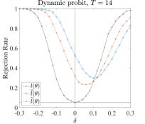
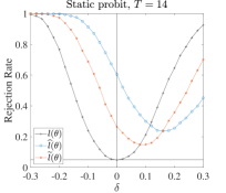
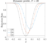
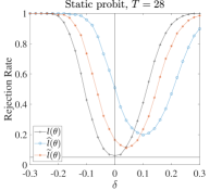
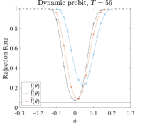
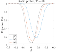
Figure G.1: Size and power of LR tests for probit model with $(\lambda+\alpha_{i}+\gamma_{t})U_{it}$

Notes: The plotted curves are the rejection rates of the LR tests based on $l\left(\theta\right)$ (+), $\widehat{l}\left(\theta\right)$ (o), and $\widetilde{l}\left(\theta\right)$ (*) calculated over $1000$ replications. The dynamic model is $Y_{it}=1\left(\rho_{0}Y_{it-1}+\beta_{0}X_{it}+\left(\delta_{0}+\alpha_{i0}+\gamma_{t0}\right)U_{it}+\varepsilon_{it}>0\right)$ with $Y_{i0}=1\left(\beta_{0}X_{i0}+\left(\lambda_{0}+\alpha_{i0}+\gamma_{00}\right)U_{i0}+\varepsilon_{i0}>0\right)$ and the static model $Y_{it}=1\left(\beta_{0}X_{it}+\left(\delta_{0}+\alpha_{i0}+\gamma_{t0}\right)U_{it}+\varepsilon_{it}>0\right)$, where the true value $\theta_{0}=\left(\rho_{0},\beta_{0},\delta_{0}\right)^{\prime}=\left(0.5,1,1\right)^{\prime}$ for the dynamic model and $\theta_{0}=\left(\beta_{0},\delta_{0}\right)^{\prime}=\left(1,1\right)^{\prime}$ for the static model respectively, $\varepsilon_{it}\sim\mathcal{N}\left(0,1\right)$, $\left\{X_{it},U_{it}\right\}\sim\mathcal{N}\left(0,1/2\right)$, and $\left\{\alpha_{i0},\gamma_{t0}\right\}=0$. $N=56$. The null is at $\theta_{0}+\delta$ where, as depicted on the horizontal axis, $\delta\in\left\{-0.3,0.28,\cdots,0.3\right\}$. The vertical line is at the true value and the horizontal at the significance level $5\%$.

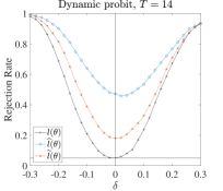
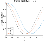
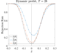
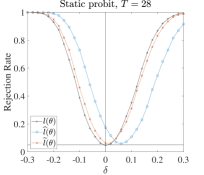
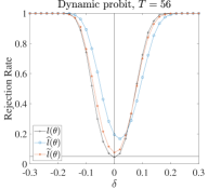
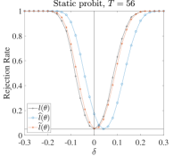
Figure G.2: Size and power of LR tests for probit model with $\alpha_{i}U_{it}+\gamma_{t}V_{it}$

Notes: The plotted curves are the rejection rates of the LR tests based on $l\left(\theta\right)$ (+), $\widehat{l}\left(\theta\right)$ (o), and $\widetilde{l}\left(\theta\right)$ (*) calculated over $1000$ replications. The dynamic model is $Y_{it}=1\left(\rho_{0}Y_{it-1}+\beta_{0}X_{it}+\alpha_{i0}U_{it}+\gamma_{t0}V_{it}+\varepsilon_{it}>0\right)$ with $Y_{i0}=1\left(\beta_{0}X_{i0}+\alpha_{i0}U_{i0}+\gamma_{00}V_{i0}+\varepsilon_{i0}>0\right)$ and the static model $Y_{it}=1\left(\beta_{0}X_{it}+\alpha_{i0}U_{it}+\gamma_{t0}V_{it}+\varepsilon_{it}>0\right)$, where the true value $\theta_{0}=\left(\rho_{0},\beta_{0}\right)^{\prime}=\left(0.5,1\right)^{\prime}$ for the dynamic model and $\theta_{0}=\beta_{0}=1$ for the static model respectively, $\varepsilon_{it}\sim\mathcal{N}\left(0,1\right)$, $X_{it}=X_{it-1}/2+\alpha_{i0}+\gamma_{t0}+\nu_{it}$ with $\nu_{it}\sim\mathcal{N}\left(0,1/2\right)$, and $\left\{\alpha_{i0},\gamma_{t0}\right\}\sim\mathcal{N}\left(0,1/16\right)$. $U_{it}$ and $V_{it}$ are generated in the same way as $X_{it}$. $N=56$. The null is at $\theta_{0}+\delta$ where, as depicted on the horizontal axis, $\delta\in\left\{-0.3,0.28,\cdots,0.3\right\}$. The vertical line is at the true value and the horizontal at the significance level $5\%$.

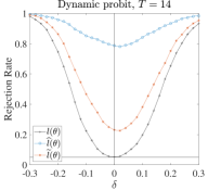
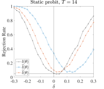
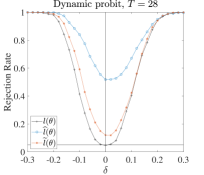
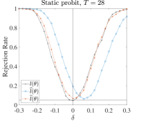
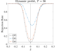
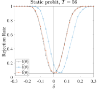
Figure G.3: Statistical power and size of LR tests for probit model with $\alpha_{i}+\gamma_{t}$

Notes: The plotted curves are the rejection rates of the LR tests based on $l\left(\theta\right)$ (+), $\widehat{l}\left(\theta\right)$ (o), and $\widetilde{l}\left(\theta\right)$ (*) calculated over $1000$ replications. $N=56$. The model is $Y_{it}=1\left(\rho_{0}Y_{it-1}+X_{it}\beta_{0}+\alpha_{i0}+\gamma_{t0}+\varepsilon_{it}>0\right)$ for the dynamic model with $Y_{i0}=1\left(\beta_{0}X_{i0}+\alpha_{i0}+\gamma_{00}+\varepsilon_{i0}>0\right)$ and $Y_{it}=1\left(X_{it}\beta_{0}+\alpha_{i0}+\gamma_{t0}+\varepsilon_{it}>0\right)$ for the static model where the true value $\theta_{0}=\left(\rho_{0},\beta_{0}\right)^{\prime}=\left(0.5,1\right)^{\prime}$ for the dynamic model and $\theta_{0}=\beta_{0}=1$ for the static model,$\ \varepsilon_{it}\sim\mathcal{N}\left(0,1\right)$, $\left\{\alpha_{i0},\gamma_{t0}\right\}\sim\mathcal{N}\left(0,1/16\right)$, and $X_{it}=X_{it-1}/2+\alpha_{i0}+\gamma_{t0}+\nu_{it}$ with $\nu_{it}\sim\mathcal{N}\left(0,1/2\right)$ and $X_{i0}\sim\mathcal{N}\left(0,1\right)$. The null is at $\theta_{0}+\delta$ where, as depicted on the horizontal axis, $\delta\in\left\{-0.3,0.28,\cdots,0.3\right\}$. The vertical line is at the true value and the horizontal at the significance level $5\%$.

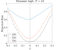
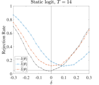
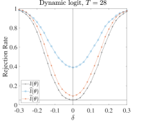
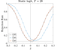
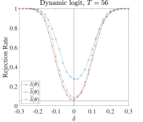
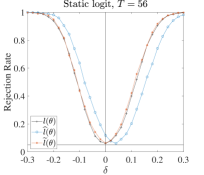
Figure G.4: Statistical power and size of LR tests for logit model with $\alpha_{i}+\gamma_{t}$

Notes: The plotted curves are the rejection rates of the LR tests based on $l\left(\theta\right)$ (+), $\widehat{l}\left(\theta\right)$ (o), and $\widetilde{l}\left(\theta\right)$ (*) calculated over $1000$ replications. $N=56$. The model is $Y_{it}=1\left(\rho_{0}Y_{it-1}+X_{it}\beta_{0}+\alpha_{i0}+\gamma_{t0}+\varepsilon_{it}>0\right)$ for the dynamic model with $Y_{i0}=1\left(\beta_{0}X_{i0}+\alpha_{i0}+\gamma_{00}+\varepsilon_{i0}>0\right)$ and $Y_{it}=1\left(X_{it}\beta_{0}+\alpha_{i0}+\gamma_{t0}+\varepsilon_{it}>0\right)$ for the static model where the true value $\theta_{0}=\left(\rho_{0},\beta_{0}\right)^{\prime}=\left(0.5,1\right)^{\prime}$ for the dynamic model and $\theta_{0}=\beta_{0}=1$ for the static model, $\varepsilon_{it}$ is standard-logistically distributed, $\left\{\alpha_{i0},\gamma_{t0}\right\}\sim\mathcal{N}\left(0,1/16\right)$, and $X_{it}=X_{it-1}/2+\alpha_{i0}+\gamma_{t0}+\nu_{it}$ with $\nu_{it}\sim\mathcal{N}\left(0,1/2\right)$ and $X_{i0}\sim\mathcal{N}\left(0,1\right)$. The null is at $\theta_{0}+\delta$ where, as depicted on the horizontal axis, $\delta\in\left\{-0.3,0.28,\cdots,0.3\right\}$. The vertical line is at the true value and the horizontal at the significance level $5\%$.

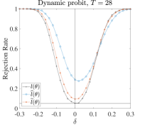
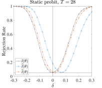
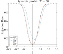
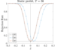
Figure G.5: Statistical power and size of LR tests for probit model with $\alpha_{i}U_{it}+\gamma_{t}$

Notes: The plotted curves are the rejection rates of the LR tests based on $l\left(\theta\right)$ (+), $\widehat{l}\left(\theta\right)$ (o), and $\widetilde{l}\left(\theta\right)$ (*) calculated over $1000$ replications. $N=56$. The model is $Y_{it}=1\left(\rho_{0}Y_{it-1}+X_{it}\beta_{0}+\alpha_{i0}W_{it}+\gamma_{t0}+\varepsilon_{it}>0\right)$ for the dynamic model with $Y_{i0}=1\left(\beta_{0}X_{i0}+\alpha_{i0}U_{i0}+\gamma_{00}+\varepsilon_{i0}>0\right)$ and $Y_{it}=1\left(X_{it}\beta_{0}+\alpha_{i0}U_{it}+\gamma_{t0}+\varepsilon_{it}>0\right)$ for the static model where the true value $\theta_{0}=\left(\rho_{0},\beta_{0}\right)^{\prime}=\left(0.5,1\right)^{\prime}$ for the dynamic model and $\theta_{0}=\beta_{0}=1$ for the static model, $\varepsilon_{it}\sim\mathcal{N}\left(0,1\right)$, $\left\{\alpha_{i0},\gamma_{t0}\right\}\sim\mathcal{N}\left(0,1/16\right)$, and $X_{it}=X_{it-1}/2+\alpha_{i0}+\gamma_{t0}+\nu_{it}$ with $\nu_{it}\sim\mathcal{N}\left(0,1/2\right)$ and $X_{i0}\sim\mathcal{N}\left(0,1\right)$. $U_{it}$ is generated in the same way as $X_{it}$. The null is at $\theta_{0}+\delta$ where, as depicted on the horizontal axis, $\delta\in\left\{-0.3,0.28,\cdots,0.3\right\}$. The vertical line is at the true value and the horizontal at the significance level $5\%$.

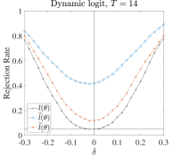
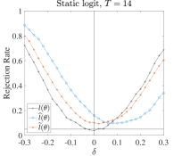
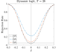
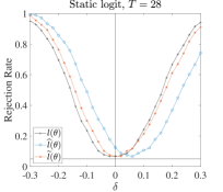
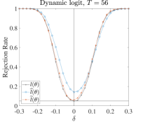
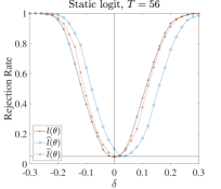
Figure G.6: Statistical power and size of LR tests for logit model with $\alpha_{i}U_{it}+\gamma_{t}$

Notes: The plotted curves are the rejection rates of the LR tests based on $l\left(\theta\right)$ (+), $\widehat{l}\left(\theta\right)$ (o), and $\widetilde{l}\left(\theta\right)$ (*) calculated over $1000$ replications. $N=56$. The model is $Y_{it}=1\left(\rho_{0}Y_{it-1}+X_{it}\beta_{0}+\alpha_{i0}U_{it}+\gamma_{t0}+\varepsilon_{it}>0\right)$ for the dynamic model with $Y_{i0}=1\left(\beta_{0}X_{i0}+\alpha_{i0}U_{i0}+\gamma_{00}+\varepsilon_{i0}>0\right)$ and $Y_{it}=1\left(X_{it}\beta_{0}+\alpha_{i0}U_{it}+\gamma_{t0}+\varepsilon_{it}>0\right)$ for the static model where the true value $\theta_{0}=\left(\rho_{0},\beta_{0}\right)^{\prime}=\left(0.5,1\right)^{\prime}$ for the dynamic model and $\theta_{0}=\beta_{0}=1$ for the static model, $\varepsilon_{it}$ is standard-logistically distributed, $\left\{\alpha_{i0},\gamma_{t0}\right\}\sim\mathcal{N}\left(0,1/16\right)$, and $X_{it}=X_{it-1}/2+\alpha_{i0}+\gamma_{t0}+\nu_{it}$ with $\nu_{it}\sim\mathcal{N}\left(0,1/2\right)$ and $X_{i0}\sim\mathcal{N}\left(0,1\right)$. $U_{it}$ is generated in the same way as $X_{it}$. The null is at $\theta_{0}+\delta$ where, as depicted on the horizontal axis, $\delta\in\left\{-0.3,0.28,\cdots,0.3\right\}$. The vertical line is at the true value and the horizontal at the significance level $5\%$.

G.2 Extra results for the LM test

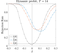
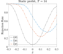
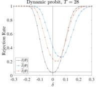
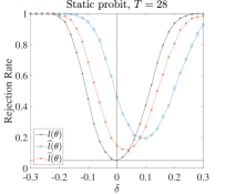
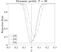
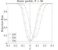
Figure G.7: Size and power of LM tests for probit model with $(\lambda_{0}+\alpha_{i}+\gamma_{t})U_{it}$

Notes: The plotted curves are the rejection rates of the LM tests based on $l\left(\theta\right)$ (+), $\widehat{l}\left(\theta\right)$ (o), and $\widetilde{l}\left(\theta\right)$ (*) calculated over $1000$ replications. The dynamic model is $Y_{it}=1\left(\rho_{0}Y_{it-1}+\beta_{0}X_{it}+\left(\lambda_{0}+\alpha_{i0}+\gamma_{t0}\right)U_{it}+\varepsilon_{it}>0\right)$ with $Y_{i0}=1\left(\beta_{0}X_{i0}+\left(\lambda_{0}+\alpha_{i0}+\gamma_{00}\right)U_{i0}+\varepsilon_{i0}>0\right)$ and the static model $Y_{it}=1\left(\beta_{0}X_{it}+\left(\lambda_{0}+\alpha_{i0}+\gamma_{t0}\right)U_{it}+\varepsilon_{it}>0\right)$, where the true value $\theta_{0}=\left(\rho_{0},\beta_{0},\delta_{0}\right)^{\prime}=\left(0.5,1,1\right)^{\prime}$ for the dynamic model and $\theta_{0}=\left(\beta_{0},\delta_{0}\right)^{\prime}=\left(1,1\right)^{\prime}$ for the static model respectively, $\varepsilon_{it}\sim\mathcal{N}\left(0,1\right)$, $\left\{X_{it},U_{it}\right\}\sim\mathcal{N}\left(0,1/2\right)$, and $\left\{\alpha_{i0},\gamma_{t0}\right\}=0$. $N=56$. The null is at $\theta_{0}+\delta$ where, as depicted on the horizontal axis, $\delta\in\left\{-0.3,0.28,\cdots,0.3\right\}$. The vertical line is at the true value and the horizontal at the significance level $5\%$.

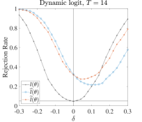
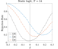
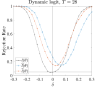
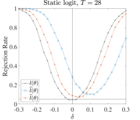
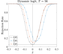
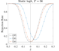
Figure G.8: Size and power of LM tests for logit model with $(\lambda+\alpha_{i}+\gamma_{t})U_{it}$

Notes: The plotted curves are the rejection rates of the LM tests based on $l\left(\theta\right)$ (+), $\widehat{l}\left(\theta\right)$ (o), and $\widetilde{l}\left(\theta\right)$ (*) calculated over $1000$ replications. The dynamic model is $Y_{it}=1\left(\rho_{0}Y_{it-1}+\beta_{0}X_{it}+\left(\lambda_{0}+\alpha_{i0}+\gamma_{t0}\right)U_{it}+\varepsilon_{it}>0\right)$ with $Y_{i0}=1\left(\beta_{0}X_{i0}+\left(\lambda_{0}+\alpha_{i0}+\gamma_{00}\right)U_{i0}+\varepsilon_{i0}>0\right)$ and the static model $Y_{it}=1\left(\beta_{0}X_{it}+\left(\lambda_{0}+\alpha_{i0}+\gamma_{t0}\right)U_{it}+\varepsilon_{it}>0\right)$, where the true value $\theta_{0}=\left(\rho_{0},\beta_{0},\delta_{0}\right)^{\prime}=\left(0.5,1,1\right)^{\prime}$ for the dynamic model and $\theta_{0}=\left(\beta_{0},\delta_{0}\right)^{\prime}=\left(1,1\right)^{\prime}$ for the static model respectively, $\varepsilon_{it}$ is standard-logistically distributed, $\left\{X_{it},U_{it}\right\}\sim\mathcal{N}\left(0,1/2\right)$, and $\left\{\alpha_{i0},\gamma_{t0}\right\}=0$. $N=56$. The null is at $\theta_{0}+\delta$ where, as depicted on the horizontal axis, $\delta\in\left\{-0.3,0.28,\cdots,0.3\right\}$. The vertical line is at the true value and the horizontal at the significance level $5\%$.

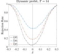
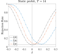
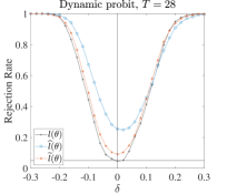
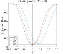
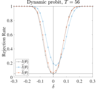
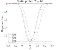
Figure G.9: Size and power of LM tests for probit model with $\alpha_{i}U_{it}+\gamma_{t}V_{it}$

Notes: The plotted curves are the rejection rates of the LM tests based on $l\left(\theta\right)$ (+), $\widehat{l}\left(\theta\right)$ (o), and $\widetilde{l}\left(\theta\right)$ (*) calculated over $1000$ replications. The dynamic model is $Y_{it}=1\left(\rho_{0}Y_{it-1}+\beta_{0}X_{it}+\alpha_{i0}U_{it}+\gamma_{t0}V_{it}+\varepsilon_{it}>0\right)$ with $Y_{i0}=1\left(\beta_{0}X_{i0}+\alpha_{i0}U_{i0}+\gamma_{00}V_{i0}+\varepsilon_{i0}>0\right)$ and the static $Y_{it}=1\left(\beta_{0}X_{it}+\alpha_{i0}U_{it}+\gamma_{t0}V_{it}+\varepsilon_{it}>0\right)$, where the true value $\theta_{0}=\left(\rho_{0},\beta_{0}\right)^{\prime}=\left(0.5,1\right)^{\prime}$ for the dynamic model and $\theta_{0}=\beta_{0}=1$ for the static model respectively, $\varepsilon_{it}\sim\mathcal{N}\left(0,1\right)$, $X_{it}=X_{it-1}/2+\alpha_{i0}+\gamma_{t0}+\nu_{it}$ with $\nu_{it}\sim\mathcal{N}\left(0,1/2\right)$, and $\left\{\alpha_{i0},\gamma_{t0}\right\}\sim\mathcal{N}\left(0,1/16\right)$. $U_{it}$ and $V_{it}$ are generated in the same way as $X_{it}$. $N=56$. The null is at $\theta_{0}+\delta$ where, as depicted on the horizontal axis, $\delta\in\left\{-0.3,0.28,\cdots,0.3\right\}$. The vertical line is at the true value and the horizontal at the significance level $5\%$.

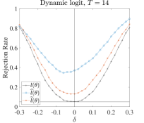
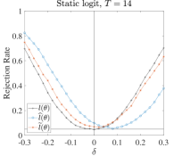
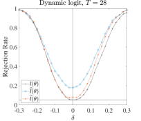
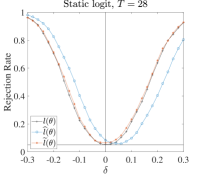
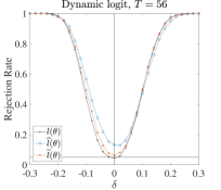
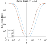
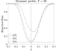
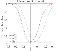
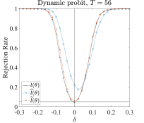
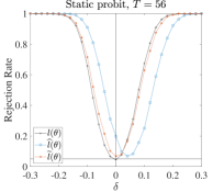
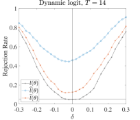
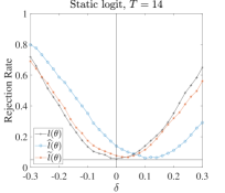
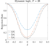
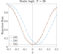
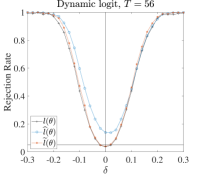
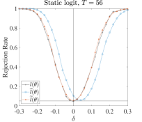
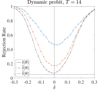
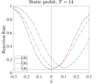
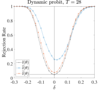
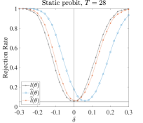
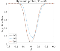
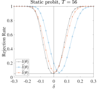
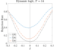
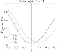
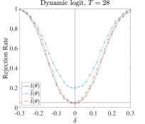
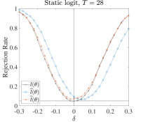
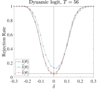
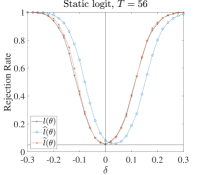
Figure G.10: Size and power of LM tests for logit model with $\alpha_{i}U_{it}+\gamma_{t}V_{it}$

Notes: The plotted curves are the rejection rates of the LM tests based on $l\left(\theta\right)$ (+), $\widehat{l}\left(\theta\right)$ (o), and $\widetilde{l}\left(\theta\right)$ (*) calculated over $1000$ replications. The dynamic model is $Y_{it}=1\left(\rho_{0}Y_{it-1}+\beta_{0}X_{it}+\alpha_{i0}U_{it}+\gamma_{t0}V_{it}+\varepsilon_{it}>0\right)$ with $Y_{i0}=1\left(\beta_{0}X_{i0}+\alpha_{i0}U_{i0}+\gamma_{00}V_{i0}+\varepsilon_{i0}>0\right)$ and the static $Y_{it}=1\left(\beta_{0}X_{it}+\alpha_{i0}U_{it}+\gamma_{t0}V_{it}+\varepsilon_{it}>0\right)$, where the true value $\theta_{0}=\left(\rho_{0},\beta_{0}\right)^{\prime}=\left(0.5,1\right)^{\prime}$ for the dynamic model and $\theta_{0}=\beta_{0}=1$ for the static model respectively, $\varepsilon_{it}$ is standard-logistically distributed, $X_{it}=X_{it-1}/2+\alpha_{i0}+\gamma_{t0}+\nu_{it}$ with $\nu_{it}\sim\mathcal{N}\left(0,1/2\right)$, and $\left\{\alpha_{i0},\gamma_{t0}\right\}\sim\mathcal{N}\left(0,1/16\right)$. $U_{it}$ and $V_{it}$ are generated in the same way as $X_{it}$. $N=56$. The null is at $\theta_{0}+\delta$ where, as depicted on the horizontal axis, $\delta\in\left\{-0.3,0.28,\cdots,0.3\right\}$. The vertical line is at the true value and the horizontal at the significance level $5\%$.

Figure G.11: Statistical power and size of LM tests for probit model with $\alpha_{i}+\gamma_{t}$

Notes: The plotted curves are the rejection rates of the LM tests based on $l\left(\theta\right)$ (+), $\widehat{l}\left(\theta\right)$ (o), and $\widetilde{l}\left(\theta\right)$ (*) calculated over $1000$ replications. $N=56$. The model is $Y_{it}=1\left(\rho_{0}Y_{it-1}+X_{it}\beta_{0}+\alpha_{i0}+\gamma_{t0}+\varepsilon_{it}>0\right)$ for the dynamic model with $Y_{i0}=1\left(\beta_{0}X_{i0}+\alpha_{i0}+\gamma_{00}+\varepsilon_{i0}>0\right)$ and $Y_{it}=1\left(X_{it}\beta_{0}+\alpha_{i0}+\gamma_{t0}+\varepsilon_{it}>0\right)$ for the static model where the true value $\theta_{0}=\left(\rho_{0},\beta_{0}\right)^{\prime}=\left(0.5,1\right)^{\prime}$ for the dynamic model and $\theta_{0}=\beta_{0}=1$ for the static model, $\varepsilon_{it}\sim\mathcal{N}\left(0,1\right)$, $\left\{\alpha_{i0},\gamma_{t0}\right\}\sim\mathcal{N}\left(0,1/16\right)$, and $X_{it}=X_{it-1}/2+\alpha_{i0}+\gamma_{t0}+\nu_{it}$ with $\nu_{it}\sim\mathcal{N}\left(0,1/2\right)$ and $X_{i0}\sim\mathcal{N}\left(0,1\right)$. The null is at $\theta_{0}+\delta$ where, as depicted on the horizontal axis, $\delta\in\left\{-0.3,0.28,\cdots,0.3\right\}$. The vertical line is at the true value and the horizontal at the significance level $5\%$.

Figure G.12: Statistical power and size of LM tests for logit model with $\alpha_{i}+\gamma_{t}$

Notes: The plotted curves are the rejection rates of the LM tests based on $l\left(\theta\right)$ (+), $\widehat{l}\left(\theta\right)$ (o), and $\widetilde{l}\left(\theta\right)$ (*) calculated over $1000$ replications. $N=56$. The model is $Y_{it}=1\left(\rho_{0}Y_{it-1}+X_{it}\beta_{0}+\alpha_{i0}+\gamma_{t0}+\varepsilon_{it}>0\right)$ for the dynamic model with $Y_{i0}=1\left(\beta_{0}X_{i0}+\alpha_{i0}+\gamma_{00}+\varepsilon_{i0}>0\right)$ and $Y_{it}=1\left(X_{it}\beta_{0}+\alpha_{i0}+\gamma_{t0}+\varepsilon_{it}>0\right)$ for the static model where the true value $\theta_{0}=\left(\rho_{0},\beta_{0}\right)^{\prime}=\left(0.5,1\right)^{\prime}$ for the dynamic model and $\theta_{0}=\beta_{0}=1$ for the static model, $\varepsilon_{it}$ is standard-logistically distributed, $\left\{\alpha_{i0},\gamma_{t0}\right\}\sim\mathcal{N}\left(0,1/16\right)$, and $X_{it}=X_{it-1}/2+\alpha_{i0}+\gamma_{t0}+\nu_{it}$ with $\nu_{it}\sim\mathcal{N}\left(0,1/2\right)$ and $X_{i0}\sim\mathcal{N}\left(0,1\right)$. The null is at $\theta_{0}+\delta$ where, as depicted on the horizontal axis, $\delta\in\left\{-0.3,0.28,\cdots,0.3\right\}$. The vertical line is at the true value and the horizontal at the significance level $5\%$.

Figure G.13: Statistical power and size of LM tests for probit model with $\alpha_{i}U_{it}+\gamma_{t}$

Notes: The plotted curves are the rejection rates of the LM tests based on $l\left(\theta\right)$ (+), $\widehat{l}\left(\theta\right)$ (o), and $\widetilde{l}\left(\theta\right)$ (*) calculated over $1000$ replications. $N=56$. The model is $Y_{it}=1\left(\rho_{0}Y_{it-1}+X_{it}\beta_{0}+\alpha_{i0}U_{it}+\gamma_{t0}+\varepsilon_{it}>0\right)$ for the dynamic model with $Y_{i0}=1\left(\beta_{0}X_{i0}+\alpha_{i0}U_{i0}+\gamma_{00}+\varepsilon_{i0}>0\right)$ and $Y_{it}=1\left(X_{it}\beta_{0}+\alpha_{i0}U_{it}+\gamma_{t0}+\varepsilon_{it}>0\right)$ for the static model where the true value $\theta_{0}=\left(\rho_{0},\beta_{0}\right)^{\prime}=\left(0.5,1\right)^{\prime}$ for the dynamic model and $\theta_{0}=\beta_{0}=1$ for the static model, $\varepsilon_{it}\sim\mathcal{N}\left(0,1\right)$, $\left\{\alpha_{i0},\gamma_{t0}\right\}\sim\mathcal{N}\left(0,1/16\right)$, and $X_{it}=X_{it-1}/2+\alpha_{i0}+\gamma_{t0}+\nu_{it}$ with $\nu_{it}\sim\mathcal{N}\left(0,1/2\right)$ and $X_{i0}\sim\mathcal{N}\left(0,1\right)$. $U_{it}$ is generated in the same way as $X_{it}$. The null is at $\theta_{0}+\delta$ where, as depicted on the horizontal axis, $\delta\in\left\{-0.3,0.28,\cdots,0.3\right\}$. The vertical line is at the true value and the horizontal at the significance level $5\%$.

Figure G.14: Statistical power and size of LM tests for logit model with $\alpha_{i}U_{it}+\gamma_{t}$

Notes: The plotted curves are the rejection rates of the LM tests based on $l\left(\theta\right)$ (+), $\widehat{l}\left(\theta\right)$ (o), and $\widetilde{l}\left(\theta\right)$ (*) calculated over $1000$ replications. $N=56$. The model is $Y_{it}=1\left(\rho_{0}Y_{it-1}+X_{it}\beta_{0}+\alpha_{i0}U_{it}+\gamma_{t0}+\varepsilon_{it}>0\right)$ for the dynamic model with $Y_{i0}=1\left(\beta_{0}X_{i0}+\alpha_{i0}U_{i0}+\gamma_{00}+\varepsilon_{i0}>0\right)$ and $Y_{it}=1\left(X_{it}\beta_{0}+\alpha_{i0}U_{it}+\gamma_{t0}+\varepsilon_{it}>0\right)$ for the static model where the true value $\theta_{0}=\left(\rho_{0},\beta_{0}\right)^{\prime}=\left(0.5,1\right)^{\prime}$ for the dynamic model and $\theta_{0}=\beta_{0}=1$ for the static model, $\varepsilon_{it}$ is standard-logistically distributed, $\left\{\alpha_{i0},\gamma_{t0}\right\}\sim\mathcal{N}\left(0,1/16\right)$, and $X_{it}=X_{it-1}/2+\alpha_{i0}+\gamma_{t0}+\nu_{it}$ with $\nu_{it}\sim\mathcal{N}\left(0,1/2\right)$ and $X_{i0}\sim\mathcal{N}\left(0,1\right)$. $U_{it}$ is generated in the same way as $X_{it}$. The null is at $\theta_{0}+\delta$ where, as depicted on the horizontal axis, $\delta\in\left\{-0.3,0.28,\cdots,0.3\right\}$. The vertical line is at the true value and the horizontal at the significance level $5\%$.

G.3 Extra results for the Wald test

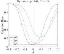
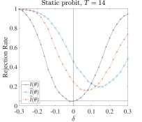
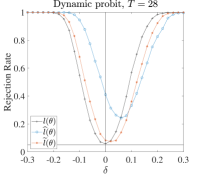
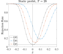
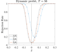
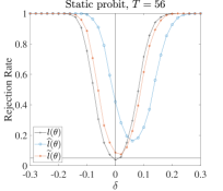
Figure G.15: Size and power of Wald tests for probit model with $(\lambda+\alpha_{i}+\gamma_{t})U_{it}$

Notes: The plotted curves are the rejection rates of the Wald tests based on $l\left(\theta\right)$ (+), $\widehat{l}\left(\theta\right)$ (o), and $\widetilde{l}\left(\theta\right)$ (*) calculated over $1000$ replications. The dynamic model is $Y_{it}=1\left(\rho_{0}Y_{it-1}+\beta_{0}X_{it}+\left(\lambda_{0}+\alpha_{i0}+\gamma_{t0}\right)U_{it}+\varepsilon_{it}>0\right)$ with $Y_{i0}=1\left(\beta_{0}X_{i0}+\left(\lambda_{0}+\alpha_{i0}+\gamma_{00}\right)U_{i0}+\varepsilon_{i0}>0\right)$ and the static model $Y_{it}=1\left(\beta_{0}X_{it}+\left(\lambda_{0}+\alpha_{i0}+\gamma_{t0}\right)U_{it}+\varepsilon_{it}>0\right)$, where the true value $\theta_{0}=\left(\rho_{0},\beta_{0},\delta_{0}\right)^{\prime}=\left(0.5,1,1\right)^{\prime}$ for the dynamic model and $\theta_{0}=\left(\beta_{0},\delta_{0}\right)^{\prime}=\left(1,1\right)^{\prime}$ for the static model respectively, $\varepsilon_{it}\sim\mathcal{N}\left(0,1\right)$, $\left\{X_{it},U_{it}\right\}\sim\mathcal{N}\left(0,1/2\right)$, and $\left\{\alpha_{i0},\gamma_{t0}\right\}=0$. $N=56$. The null is at $\theta_{0}+\delta$ where, as depicted on the horizontal axis, $\delta\in\left\{-0.3,0.28,\cdots,0.3\right\}$. The vertical line is at the true value and the horizontal at the significance level $5\%$.

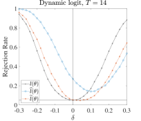
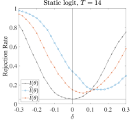
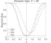
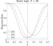
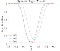
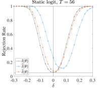
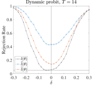
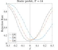
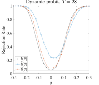
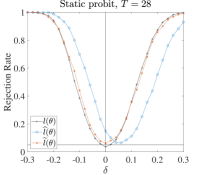
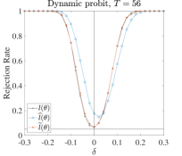
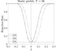
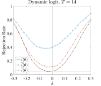
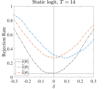
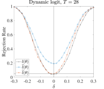
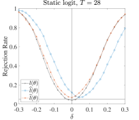
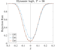
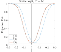
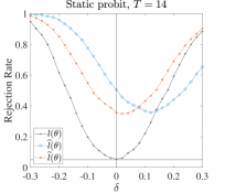
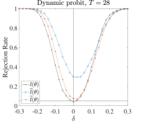
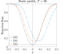
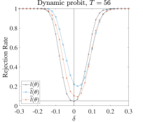
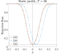
Figure G.16: Size and power of Wald tests for logit model with $(\lambda+\alpha_{i}+\gamma_{t})U_{it}$

Notes: The plotted curves are the rejection rates of the Wald tests based on $l\left(\theta\right)$ (+), $\widehat{l}\left(\theta\right)$ (o), and $\widetilde{l}\left(\theta\right)$ (*) calculated over $1000$ replications. The dynamic model is $Y_{it}=1\left(\rho_{0}Y_{it-1}+\beta_{0}X_{it}+\left(\lambda_{0}+\alpha_{i0}+\gamma_{t0}\right)U_{it}+\varepsilon_{it}>0\right)$ with $Y_{i0}=1\left(\beta_{0}X_{i0}+\left(\lambda_{0}+\alpha_{i0}+\gamma_{00}\right)U_{i0}+\varepsilon_{i0}>0\right)$ and the static model $Y_{it}=1\left(\beta_{0}X_{it}+\left(\lambda_{0}+\alpha_{i0}+\gamma_{t0}\right)U_{it}+\varepsilon_{it}>0\right)$, where the true value $\theta_{0}=\left(\rho_{0},\beta_{0},\delta_{0}\right)^{\prime}=\left(0.5,1,1\right)^{\prime}$ for the dynamic model and $\theta_{0}=\left(\beta_{0},\delta_{0}\right)^{\prime}=\left(1,1\right)^{\prime}$ for the static model respectively, $\varepsilon_{it}$ is standard-logistically distributed, $\left\{X_{it},U_{it}\right\}\sim\mathcal{N}\left(0,1/2\right)$, and $\left\{\alpha_{i0},\gamma_{t0}\right\}=0$. $N=56$. The null is at $\theta_{0}+\delta$ where, as depicted on the horizontal axis, $\delta\in\left\{-0.3,0.28,\cdots,0.3\right\}$. The vertical line is at the true value and the horizontal at the significance level $5\%$.

Figure G.17: Size and power of Wald tests for probit model with $\alpha_{i}U_{it}+\gamma_{t}V_{it}$

Notes: The plotted curves are the rejection rates of the Wald tests based on $l\left(\theta\right)$ (+), $\widehat{l}\left(\theta\right)$ (o), and $\widetilde{l}\left(\theta\right)$ (*) calculated over $1000$ replications. The dynamic model is $Y_{it}=1\left(\rho_{0}Y_{it-1}+\beta_{0}X_{it}+\alpha_{i0}U_{it}+\gamma_{t0}V_{it}+\varepsilon_{it}>0\right)$ with $Y_{i0}=1\left(\beta_{0}X_{i0}+\alpha_{i0}U_{i0}+\gamma_{00}V_{i0}+\varepsilon_{i0}>0\right)$ and the static $Y_{it}=1\left(\beta_{0}X_{it}+\alpha_{i0}U_{it}+\gamma_{t0}V_{it}+\varepsilon_{it}>0\right)$, where the true value $\theta_{0}=\left(\rho_{0},\beta_{0}\right)^{\prime}=\left(0.5,1\right)^{\prime}$ for the dynamic model and $\theta_{0}=\beta_{0}=1$ for the static model respectively, $\varepsilon_{it}\sim\mathcal{N}\left(0,1\right)$, $X_{it}=X_{it-1}/2+\alpha_{i0}+\gamma_{t0}+\nu_{it}$ with $\nu_{it}\sim\mathcal{N}\left(0,1/2\right)$, and $\left\{\alpha_{i0},\gamma_{t0}\right\}\sim\mathcal{N}\left(0,1/16\right)$. $U_{it}$ and $V_{it}$ are generated in the same way as $X_{it}$. $N=56$. The null is at $\theta_{0}+\delta$ where, as depicted on the horizontal axis, $\delta\in\left\{-0.3,0.28,\cdots,0.3\right\}$. The vertical line is at the true value and the horizontal at the significance level $5\%$.

Figure G.18: Size and power of Wald tests for logit model with $\alpha_{i}U_{it}+\gamma_{t}V_{it}$

Notes: The plotted curves are the rejection rates of the Wald tests based on $l\left(\theta\right)$ (+), $\widehat{l}\left(\theta\right)$ (o), and $\widetilde{l}\left(\theta\right)$ (*) calculated over $1000$ replications. The dynamic model is $Y_{it}=1\left(\rho_{0}Y_{it-1}+\beta_{0}X_{it}+\alpha_{i0}U_{it}+\gamma_{t0}V_{it}+\varepsilon_{it}>0\right)$ with $Y_{i0}=1\left(\beta_{0}X_{i0}+\alpha_{i0}U_{i0}+\gamma_{00}V_{i0}+\varepsilon_{i0}>0\right)$ and the static $Y_{it}=1\left(\beta_{0}X_{it}+\alpha_{i0}U_{it}+\gamma_{t0}V_{it}+\varepsilon_{it}>0\right)$, where the true value $\theta_{0}=\left(\rho_{0},\beta_{0}\right)^{\prime}=\left(0.5,1\right)^{\prime}$ for the dynamic model and $\theta_{0}=\beta_{0}=1$ for the static model respectively, $\varepsilon_{it}$ is standard-logistically distributed, $X_{it}=X_{it-1}/2+\alpha_{i0}+\gamma_{t0}+\nu_{it}$ with $\nu_{it}\sim\mathcal{N}\left(0,1/2\right)$, and $\left\{\alpha_{i0},\gamma_{t0}\right\}\sim\mathcal{N}\left(0,1/16\right)$. $U_{it}$ and $V_{it}$ are generated in the same way as $X_{it}$. $N=56$. The null is at $\theta_{0}+\delta$ where, as depicted on the horizontal axis, $\delta\in\left\{-0.3,0.28,\cdots,0.3\right\}$. The vertical line is at the true value and the horizontal at the significance level $5\%$.

Figure G.19: Statistical power and size of Wald tests for probit model with $\alpha_{i}+\gamma_{t}$

Notes: The plotted curves are the rejection rates of the Wald tests based on $l\left(\theta\right)$ (+), $\widehat{l}\left(\theta\right)$ (o), and $\widetilde{l}\left(\theta\right)$ (*) calculated over $1000$ replications. $N=56$. The model is $Y_{it}=1\left(\rho_{0}Y_{it-1}+X_{it}\beta_{0}+\alpha_{i0}+\gamma_{t0}+\varepsilon_{it}>0\right)$ for the dynamic model with $Y_{i0}=1\left(\beta_{0}X_{i0}+\alpha_{i0}+\gamma_{00}+\varepsilon_{i0}>0\right)$ and $Y_{it}=1\left(X_{it}\beta_{0}+\alpha_{i0}+\gamma_{t0}+\varepsilon_{it}>0\right)$ for the static model where the true value $\theta_{0}=\left(\rho_{0},\beta_{0}\right)^{\prime}=\left(0.5,1\right)^{\prime}$ for the dynamic model and $\theta_{0}=\beta_{0}=1$ for the static model,$\ \varepsilon_{it}\sim\mathcal{N}\left(0,1\right)$, $\left\{\alpha_{i0},\gamma_{t0}\right\}\sim\mathcal{N}\left(0,1/16\right)$, and $X_{it}=X_{it-1}/2+\alpha_{i0}+\gamma_{t0}+\nu_{it}$ with $\nu_{it}\sim\mathcal{N}\left(0,1/2\right)$ and $X_{i0}\sim\mathcal{N}\left(0,1\right)$. The null is at $\theta_{0}+\delta$ where, as depicted on the horizontal axis, $\delta\in\left\{-0.3,0.28,\cdots,0.3\right\}$. The vertical line is at the true value and the horizontal at the significance level $5\%$.

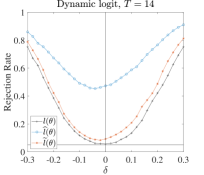
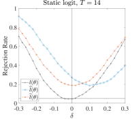
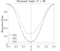
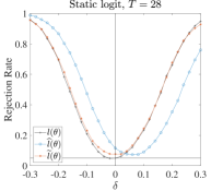
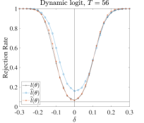
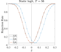
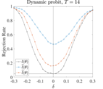
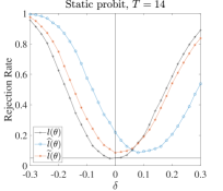
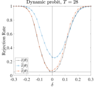
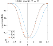
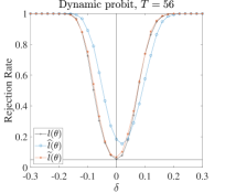
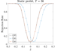
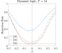
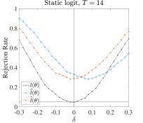
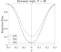
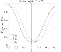
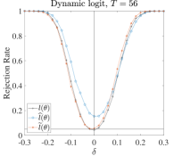
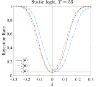
Figure G.20: Statistical power and size of Wald tests for logit model with $\alpha_{i}+\gamma_{t}$

Notes: The plotted curves are the rejection rates of the Wald tests based on $l\left(\theta\right)$ (+), $\widehat{l}\left(\theta\right)$ (o), and $\widetilde{l}\left(\theta\right)$ (*) calculated over $1000$ replications. $N=56$. The model is $Y_{it}=1\left(\rho_{0}Y_{it-1}+X_{it}\beta_{0}+\alpha_{i0}+\gamma_{t0}+\varepsilon_{it}>0\right)$ for the dynamic model with $Y_{i0}=1\left(\beta_{0}X_{i0}+\alpha_{i0}+\gamma_{00}+\varepsilon_{i0}>0\right)$ and $Y_{it}=1\left(X_{it}\beta_{0}+\alpha_{i0}+\gamma_{t0}+\varepsilon_{it}>0\right)$ for the static model where the true value $\theta_{0}=\left(\rho_{0},\beta_{0}\right)^{\prime}=\left(0.5,1\right)^{\prime}$ for the dynamic model and $\theta_{0}=\beta_{0}=1$ for the static model, $\varepsilon_{it}$ is standard-logistically distributed, $\left\{\alpha_{i0},\gamma_{t0}\right\}\sim\mathcal{N}\left(0,1/16\right)$, and $X_{it}=X_{it-1}/2+\alpha_{i0}+\gamma_{t0}+\nu_{it}$ with $\nu_{it}\sim\mathcal{N}\left(0,1/2\right)$ and $X_{i0}\sim\mathcal{N}\left(0,1\right)$. The null is at $\theta_{0}+\delta$ where, as depicted on the horizontal axis, $\delta\in\left\{-0.3,0.28,\cdots,0.3\right\}$. The vertical line is at the true value and the horizontal at the significance level $5\%$.

Figure G.21: Statistical power and size of Wald tests for probit model with $\alpha_{i}U_{it}+\gamma_{t}$

Notes: The plotted curves are the rejection rates of the Wald tests based on $l\left(\theta\right)$ (+), $\widehat{l}\left(\theta\right)$ (o), and $\widetilde{l}\left(\theta\right)$ (*) calculated over $1000$ replications. $N=56$. The model is $Y_{it}=1\left(\rho_{0}Y_{it-1}+X_{it}\beta_{0}+\alpha_{i0}U_{it}+\gamma_{t0}+\varepsilon_{it}>0\right)$ for the dynamic model with $Y_{i0}=1\left(\beta_{0}X_{i0}+\alpha_{i0}U_{i0}+\gamma_{00}+\varepsilon_{i0}>0\right)$ and $Y_{it}=1\left(X_{it}\beta_{0}+\alpha_{i0}U_{it}+\gamma_{t0}+\varepsilon_{it}>0\right)$ for the static model where the true value $\theta_{0}=\left(\rho_{0},\beta_{0}\right)^{\prime}=\left(0.5,1\right)^{\prime}$ for the dynamic model and $\theta_{0}=\beta_{0}=1$ for the static model,$\ \varepsilon_{it}\sim\mathcal{N}\left(0,1\right)$, $\left\{\alpha_{i0},\gamma_{t0}\right\}\sim\mathcal{N}\left(0,1/16\right)$, and $X_{it}=X_{it-1}/2+\alpha_{i0}+\gamma_{t0}+\nu_{it}$ with $\nu_{it}\sim\mathcal{N}\left(0,1/2\right)$ and $X_{i0}\sim\mathcal{N}\left(0,1\right)$. $U_{it}$ is generated in the same way as $X_{it}$. The null is at $\theta_{0}+\delta$ where, as depicted on the horizontal axis, $\delta\in\left\{-0.3,0.28,\cdots,0.3\right\}$. The vertical line is at the true value and the horizontal at the significance level $5\%$.

Figure G.22: Statistical power and size of Wald tests for logit model with $\alpha_{i}U_{it}+\gamma_{t}$

Notes: The plotted curves are the rejection rates of the Wald tests based on $l\left(\theta\right)$ (+), $\widehat{l}\left(\theta\right)$ (o), and $\widetilde{l}\left(\theta\right)$ (*) calculated over $1000$ replications. $N=56$. The model is $Y_{it}=1\left(\rho_{0}Y_{it-1}+X_{it}\beta_{0}+\alpha_{i0}U_{it}+\gamma_{t0}+\varepsilon_{it}>0\right)$ for the dynamic model with $Y_{i0}=1\left(\beta_{0}X_{i0}+\alpha_{i0}U_{i0}+\gamma_{00}+\varepsilon_{i0}>0\right)$ and $Y_{it}=1\left(X_{it}\beta_{0}+\alpha_{i0}U_{it}+\gamma_{t0}+\varepsilon_{it}>0\right)$ for the static model where the true value $\theta_{0}=\left(\rho_{0},\beta_{0}\right)^{\prime}=\left(0.5,1\right)^{\prime}$ for the dynamic model and $\theta_{0}=\beta_{0}=1$ for the static model, $\varepsilon_{it}$ is standard-logistically distributed, $\left\{\alpha_{i0},\gamma_{t0}\right\}\sim\mathcal{N}\left(0,1/16\right)$, and $X_{it}=X_{it-1}/2+\alpha_{i0}+\gamma_{t0}+\nu_{it}$ with $\nu_{it}\sim\mathcal{N}\left(0,1/2\right)$ and $X_{i0}\sim\mathcal{N}\left(0,1\right)$. $U_{it}$ is generated in the same way as $X_{it}$. The null is at $\theta_{0}+\delta$ where, as depicted on the horizontal axis, $\delta\in\left\{-0.3,0.28,\cdots,0.3\right\}$. The vertical line is at the true value and the horizontal at the significance level $5\%$.

G.4 Bias correction on estimators

[c]

Bias-corrected probit estimates with $\alpha_{i}+\gamma_{t}$, $N=56$

		$T=14$				$T=28$				$T=56$
		Mean	Bias	RMSE		Mean	Bias	RMSE		Mean	Bias	RMSE
		Dynamic model
$\widehat{\rho}$		$0.265$	$-46.98\%$	$0.277$		$0.399$	$-20.22\%$	$0.140$		$0.454$	$-9.24\%$	$0.078$
$\widetilde{\rho}_{1}$		$0.456$	$-8.78\%$	$0.131$		$0.486$	$-2.74\%$	$0.091$		$0.494$	$-1.22\%$	$0.061$
$\widetilde{\rho}_{2}$		$0.482$	$-3.51\%$	$0.128$		$0.500$	$0.06\%$	$0.092$		$0.501$	$0.23\%$	$0.061$
$\widehat{\beta}$		$1.182$	$18.19\%$	$0.220$		$1.098$	$9.76\%$	$0.123$		$1.058$	$5.76\%$	$0.077$
$\widetilde{\beta}_{1}$		$1.006$	$0.57\%$	$0.097$		$1.006$	$0.63\%$	$0.067$		$1.005$	$0.46\%$	$0.049$
$\widetilde{\beta}_{2}$		$0.998$	$-0.17\%$	$0.095$		$1.003$	$0.33\%$	$0.067$		$1.003$	$0.34\%$	$0.048$
		Static model
$\widehat{\beta}$		$1.132$	$13.23\%$	$0.169$		$1.074$	$7.36\%$	$0.101$		$1.046$	$4.59\%$	$0.065$
$\widetilde{\beta}$		$1.008$	$0.76\%$	$0.088$		$1.004$	$0.44\%$	$0.062$		$1.002$	$0.19\%$	$0.044$

• Notes: The number of replications is $1000$. Mean is the monte-carlo mean of the estimates. Bias is the percentage bias of the estimates relatively to the true value. RMSE is the root mean squared error. $\widehat{\rho}$ and $\widehat{\beta}$ are the uncorrected estimators of $\rho_{0}$ and $\beta_{0}$ respectively; $\widetilde{\rho}_{\tau}$ and $\widetilde{\beta}_{\tau}$ are the bias-corrected estimators using $\widetilde{l}\left(\theta\right)$ (without $\mathbb{E}\partial_{\alpha_{i}}l_{it}(\theta,\widehat{\phi}(\theta))$ and $\mathbb{E}\partial_{\gamma_{t}}l_{it}(\theta,\widehat{\phi}(\theta))$) and setting the truncation parameter at $\tau$ (for dynamic model only). $N=56$. The model is $Y_{it}=1\left(\rho_{0}Y_{it-1}+X_{it}\beta_{0}+\alpha_{i0}+\gamma_{t0}+\varepsilon_{it}>0\right)$ for dynamic model with $Y_{i0}=1\left(\beta_{0}X_{i0}+\alpha_{i0}+\gamma_{00}+\varepsilon_{i0}>0\right)$ and $Y_{it}=1\left(X_{it}\beta_{0}+\alpha_{i0}+\gamma_{t0}+\varepsilon_{it}>0\right)$ for static model where the true value $\theta_{0}=\left(\rho_{0},\beta_{0}\right)^{\prime}=\left(0.5,1\right)^{\prime}$ for the dynamic model and $\theta_{0}=\beta_{0}=1$ for the static model,$\varepsilon_{it}$ is standard-normally distributed, $\left\{\alpha_{i0},\gamma_{t0},\gamma_{00}\right\}\sim\mathcal{N}\left(0,1/16\right)$, and $X_{it}=X_{it-1}/2+\alpha_{i0}+\gamma_{t0}+\nu_{it}$ with $\nu_{it}\sim\mathcal{N}\left(0,1/2\right)$ and $X_{i0}\sim\mathcal{N}\left(0,1\right)$.

[c]

Bias-corrected logit estimates with $\alpha_{i}+\gamma_{t}$, $N=56$

		$T=14$				$T=28$				$T=56$
		Mean	Bias	RMSE		Mean	Bias	RMSE		Mean	Bias	RMSE
		Dynamic model
$\widehat{\rho}$		$0.138$	$-72.32\%$	$0.410$		$0.335$	$-33.08\%$	$0.213$		$0.424$	$-15.20\%$	$0.122$
$\widetilde{\rho}_{1}$		$0.457$	$-8.55\%$	$0.172$		$0.484$	$-3.25\%$	$0.125$		$0.491$	$-1.71\%$	$0.092$
$\widetilde{\rho}_{2}$		$0.481$	$-3.85\%$	$0.175$		$0.498$	$-0.42\%$	$0.128$		$0.499$	$-0.15\%$	$0.093$
$\widehat{\beta}$		$1.154$	$15.36\%$	$0.214$		$1.092$	$9.15\%$	$0.131$		$1.053$	$5.29\%$	$0.084$
$\widetilde{\beta}_{1}$		$0.989$	$-1.14\%$	$0.127$		$1.002$	$0.25\%$	$0.087$		$0.998$	$-0.17\%$	$0.063$
$\widetilde{\beta}_{2}$		$0.987$	$-1.34\%$	$0.127$		$1.001$	$0.10\%$	$0.087$		$0.997$	$-0.25\%$	$0.063$
		Static model
$\widehat{\beta}$		$1.114$	$11.40\%$	$0.183$		$1.065$	$6.46\%$	$0.112$		$1.042$	$4.21\%$	$0.076$
$\widetilde{\beta}$		$0.990$	$-0.99\%$	$0.128$		$0.994$	$-0.61\%$	$0.086$		$0.996$	$-0.44\%$	$0.061$

• Notes: The number of replications is $1000$. Mean is the monte-carlo mean of the estimates. Bias is the percentage bias of the estimates relatively to the true value. RMSE is the root mean squared error. $\widehat{\rho}$ and $\widehat{\beta}$ are the uncorrected estimators of $\rho_{0}$ and $\beta_{0}$ respectively; $\widetilde{\rho}_{\tau}$ and $\widetilde{\beta}_{\tau}$ are the bias-corrected estimators using $\widetilde{l}\left(\theta\right)$ (without $\mathbb{E}\partial_{\alpha_{i}}l_{it}(\theta,\widehat{\phi}(\theta))$ and $\mathbb{E}\partial_{\gamma_{t}}l_{it}(\theta,\widehat{\phi}(\theta))$) and setting the truncation parameter at $\tau$ (for dynamic model only). $N=56$. The model is $Y_{it}=1\left(\rho_{0}Y_{it-1}+X_{it}\beta_{0}+\alpha_{i0}+\gamma_{t0}+\varepsilon_{it}>0\right)$ for dynamic model with $Y_{i0}=1\left(\beta_{0}X_{i0}+\alpha_{i0}+\gamma_{00}+\varepsilon_{i0}>0\right)$ and $Y_{it}=1\left(X_{it}\beta_{0}+\alpha_{i0}+\gamma_{t0}+\varepsilon_{it}>0\right)$ for static model where the true value $\theta_{0}=\left(\rho_{0},\beta_{0}\right)^{\prime}=\left(0.5,1\right)^{\prime}$ for the dynamic model and $\theta_{0}=\beta_{0}=1$ for the static model,$\varepsilon_{it}$ is standard-logistically distributed, $\left\{\alpha_{i0},\gamma_{t0},\gamma_{00}\right\}\sim\mathcal{N}\left(0,1/16\right)$, and $X_{it}=X_{it-1}/2+\alpha_{i0}+\gamma_{t0}+\nu_{it}$ with $\nu_{it}\sim\mathcal{N}\left(0,1/2\right)$ and $X_{i0}\sim\mathcal{N}\left(0,1\right)$.

[c]

Bias-corrected probit estimates with $\alpha_{i}U_{it}+\gamma_{t}$, $N=56$

		$T=14$				$T=28$				$T=56$
		Mean	Bias	RMSE		Mean	Bias	RMSE		Mean	Bias	RMSE
		Dynamic model
$\widehat{\rho}$		$0.279$	$-44.16\%$	$0.266$		$0.402$	$-19.59\%$	$0.139$		$0.463$	$-7.50\%$	$0.076$
$\widetilde{\rho}_{1}$		$0.461$	$-7.85\%$	$0.133$		$0.477$	$-4.65\%$	$0.094$		$0.489$	$-2.16\%$	$0.064$
$\widetilde{\rho}_{2}$		$0.484$	$-3.17\%$	$0.132$		$0.489$	$-2.23\%$	$0.093$		$0.495$	$-0.90\%$	$0.064$
$\widehat{\beta}$		$1.162$	$16.18\%$	$0.205$		$1.091$	$9.12\%$	$0.119$		$1.056$	$5.56\%$	$0.074$
$\widetilde{\beta}_{1}$		$0.997$	$-0.29\%$	$0.098$		$1.002$	$0.24\%$	$0.067$		$1.000$	$0.01\%$	$0.045$
$\widetilde{\beta}_{2}$		$0.991$	$-0.94\%$	$0.098$		$1.000$	$-0.05\%$	$0.067$		$0.999$	$-0.11\%$	$0.045$
		Static model
$\widehat{\beta}$		$1.118$	$11.78\%$	$0.158$		$1.067$	$6.75\%$	$0.096$		$1.042$	$4.19\%$	$0.063$
$\widetilde{\beta}$		$1.002$	$0.18\%$	$0.088$		$1.001$	$0.07\%$	$0.062$		$0.997$	$-0.26\%$	$0.044$

• Notes: The number of replications is $1000$. Mean is the monte-carlo mean of the estimates. Bias is the percentage bias of the estimates relatively to the true value. RMSE is the root mean squared error. $\widehat{\rho}$ and $\widehat{\beta}$ are the uncorrected estimators of $\rho_{0}$ and $\beta_{0}$ respectively; $\widetilde{\rho}_{\tau}$ and $\widetilde{\beta}_{\tau}$ are the bias-corrected estimators using $\widetilde{l}\left(\theta\right)$ (without $\mathbb{E}\partial_{\alpha_{i}}l_{it}(\theta,\widehat{\phi}(\theta))$ and $\mathbb{E}\partial_{\gamma_{t}}l_{it}(\theta,\widehat{\phi}(\theta))$) and setting the truncation parameter at $\tau$ (for dynamic model only). $N=56$. The model is $Y_{it}=1\left(\rho_{0}Y_{it-1}+X_{it}\beta_{0}+\alpha_{i0}U_{it}+\gamma_{t0}+\varepsilon_{it}>0\right)$ for dynamic model with $Y_{i0}=1\left(\beta_{0}X_{i0}+\alpha_{i0}U_{i0}+\gamma_{00}+\varepsilon_{i0}>0\right)$ and $Y_{it}=1\left(X_{it}\beta_{0}+\alpha_{i0}U_{it}+\gamma_{t0}+\varepsilon_{it}>0\right)$ for static model where the true value $\theta_{0}=\left(\rho_{0},\beta_{0}\right)^{\prime}=\left(0.5,1\right)^{\prime}$ for the dynamic model and $\theta_{0}=\beta_{0}=1$ for the static model,$\varepsilon_{it}$ is standard-normally distributed, $\left\{\alpha_{i0},\gamma_{t0},\gamma_{00}\right\}\sim\mathcal{N}\left(0,1/16\right)$, and $X_{it}=X_{it-1}/2+\alpha_{i0}+\gamma_{t0}+\nu_{it}$ with $\nu_{it}\sim\mathcal{N}\left(0,1/2\right)$ and $X_{i0}\sim\mathcal{N}\left(0,1\right)$. $U_{it}$ is generated in the same way as $X_{it}$.

[c]

Bias-corrected logit estimates with $\alpha_{i}U_{it}+\gamma_{t}$, $N=56$

		$T=14$				$T=28$				$T=56$
		Mean	Bias	RMSE		Mean	Bias	RMSE		Mean	Bias	RMSE
		Dynamic model
$\widehat{\rho}$		$0.157$	$-68.58\%$	$0.397$		$0.355$	$-28.93\%$	$0.197$		$0.430$	$-14.04\%$	$0.118$
$\widetilde{\rho}_{1}$		$0.451$	$-9.75\%$	$0.180$		$0.484$	$-3.22\%$	$0.126$		$0.484$	$-3.16\%$	$0.092$
$\widetilde{\rho}_{2}$		$0.474$	$-5.15\%$	$0.182$		$0.497$	$-0.65\%$	$0.128$		$0.491$	$-1.86\%$	$0.093$
$\widehat{\beta}$		$1.140$	$14.03\%$	$0.205$		$1.071$	$7.10\%$	$0.118$		$1.047$	$4.71\%$	$0.078$
$\widetilde{\beta}_{1}$		$0.992$	$-0.85\%$	$0.128$		$0.989$	$-1.10\%$	$0.087$		$0.994$	$-0.55\%$	$0.060$
$\widetilde{\beta}_{2}$		$0.988$	$-1.17\%$	$0.128$		$0.988$	$-1.24\%$	$0.087$		$0.994$	$-0.62\%$	$0.060$
		Static model
$\widehat{\beta}$		$1.099$	$9.90\%$	$0.168$		$1.060$	$5.97\%$	$0.110$		$1.037$	$3.71\%$	$0.071$
$\widetilde{\beta}$		$0.990$	$-0.97\%$	$0.120$		$0.996$	$-0.42\%$	$0.086$		$0.994$	$-0.63\%$	$0.058$

• Notes: The number of replications is $1000$. Mean is the monte-carlo mean of the estimates. Bias is the percentage bias of the estimates relatively to the true value. RMSE is the root mean squared error. $\widehat{\rho}$ and $\widehat{\beta}$ are the uncorrected estimators of $\rho_{0}$ and $\beta_{0}$ respectively; $\widetilde{\rho}_{\tau}$ and $\widetilde{\beta}_{\tau}$ are the bias-corrected estimators using $\widetilde{l}\left(\theta\right)$ (without $\mathbb{E}\partial_{\alpha_{i}}l_{it}(\theta,\widehat{\phi}(\theta))$ and $\mathbb{E}\partial_{\gamma_{t}}l_{it}(\theta,\widehat{\phi}(\theta))$) and setting the truncation parameter at $\tau$ (for dynamic model only). $N=56$. The model is $Y_{it}=1\left(\rho_{0}Y_{it-1}+X_{it}\beta_{0}+\alpha_{i0}U_{it}+\gamma_{t0}+\varepsilon_{it}>0\right)$ for dynamic model with $Y_{i0}=1\left(\beta_{0}X_{i0}+\alpha_{i0}U_{i0}+\gamma_{00}+\varepsilon_{i0}>0\right)$ and $Y_{it}=1\left(X_{it}\beta_{0}+\alpha_{i0}U_{it}+\gamma_{t0}+\varepsilon_{it}>0\right)$ for static model where the true value $\theta_{0}=\left(\rho_{0},\beta_{0}\right)^{\prime}=\left(0.5,1\right)^{\prime}$ for the dynamic model and $\theta_{0}=\beta_{0}=1$ for the static model,$\varepsilon_{it}$ is standard-logistically distributed, $\left\{\alpha_{i0},\gamma_{t0},\gamma_{00}\right\}\sim\mathcal{N}\left(0,1/16\right)$, and $X_{it}=X_{it-1}/2+\alpha_{i0}+\gamma_{t0}+\nu_{it}$ with $\nu_{it}\sim\mathcal{N}\left(0,1/2\right)$ and $X_{i0}\sim\mathcal{N}\left(0,1\right)$. $U_{it}$ is generated in the same way as $X_{it}$.

[c]

Bias-corrected probit estimates with $\alpha_{i}U_{it}+\gamma_{t}V_{it}$, $N=56$

		$T=14$				$T=28$				$T=56$
		Mean	Bias	RMSE		Mean	Bias	RMSE		Mean	Bias	RMSE
		Dynamic model
$\widehat{\rho}$		$0.299$	$-40.20\%$	$0.245$		$0.416$	$-16.83\%$	$0.124$		$0.465$	$-6.98\%$	$0.073$
$\widetilde{\rho}_{1}$		$0.463$	$-7.38\%$	$0.123$		$0.484$	$-3.19\%$	$0.084$		$0.490$	$-1.97\%$	$0.062$
$\widetilde{\rho}_{2}$		$0.483$	$-3.30\%$	$0.121$		$0.495$	$-1.08\%$	$0.084$		$0.496$	$-0.89\%$	$0.062$
$\widehat{\beta}$		$1.164$	$16.39\%$	$0.204$		$1.086$	$8.62\%$	$0.113$		$1.054$	$5.43\%$	$0.073$
$\widetilde{\beta}_{1}$		$1.003$	$0.27\%$	$0.094$		$1.000$	$0.02\%$	$0.064$		$1.001$	$0.10\%$	$0.045$
$\widetilde{\beta}_{2}$		$0.997$	$-0.35\%$	$0.093$		$0.998$	$-0.24\%$	$0.063$		$1.000$	$0.00\%$	$0.045$
		Static model
$\widehat{\beta}$		$1.124$	$12.40\%$	$0.170$		$1.067$	$6.67\%$	$0.094$		$1.043$	$4.34\%$	$0.063$
$\widetilde{\beta}$		$1.007$	$0.73\%$	$0.095$		$1.001$	$0.14\%$	$0.060$		$1.000$	$0.03\%$	$0.043$

• Notes: The number of replications is $1000$. Mean is the monte-carlo mean of the estimates. Bias is the percentage bias of the estimates relatively to the true value. RMSE is the root mean squared error. $\widehat{\rho}$ and $\widehat{\beta}$ are the uncorrected estimators of $\rho_{0}$ and $\beta_{0}$ respectively; $\widetilde{\rho}_{\tau}$ and $\widetilde{\beta}_{\tau}$ are the bias-corrected estimators using $\widetilde{l}\left(\theta\right)$ (without $\mathbb{E}\partial_{\alpha_{i}}l_{it}(\theta,\widehat{\phi}(\theta))$ and $\mathbb{E}\partial_{\gamma_{t}}l_{it}(\theta,\widehat{\phi}(\theta))$) and setting the truncation parameter at $\tau$ (for dynamic model only). $N=56$. The model is $Y_{it}=1\left(\rho_{0}Y_{it-1}+X_{it}\beta_{0}+\alpha_{i0}U_{it}+\gamma_{t0}V_{it}+\varepsilon_{it}>0\right)$ for dynamic model with $Y_{i0}=1\left(\beta_{0}X_{i0}+\alpha_{i0}U_{i0}+\gamma_{00}V_{i0}+\varepsilon_{i0}>0\right)$ and $Y_{it}=1\left(X_{it}\beta_{0}+\alpha_{i0}U_{it}+\gamma_{t0}V_{it}+\varepsilon_{it}>0\right)$ for static model where the true value $\theta_{0}=\left(\rho_{0},\beta_{0}\right)^{\prime}=\left(0.5,1\right)^{\prime}$ for the dynamic model and $\theta_{0}=\beta_{0}=1$ for the static model,$\varepsilon_{it}$ is standard-normally distributed, $\left\{\alpha_{i0},\gamma_{t0},\gamma_{00}\right\}\sim\mathcal{N}\left(0,1/16\right)$, and $X_{it}=X_{it-1}/2+\alpha_{i0}+\gamma_{t0}+\nu_{it}$ with $\nu_{it}\sim\mathcal{N}\left(0,1/2\right)$ and $X_{i0}\sim\mathcal{N}\left(0,1\right)$. $U_{it}$ and $V_{it}$ are generated in the same way as $X_{it}$.

[c]

Bias-corrected logit estimates with $\alpha_{i}U_{it}+\gamma_{t}V_{it}$, $N=56$

		$T=14$				$T=28$				$T=56$
		Mean	Bias	RMSE		Mean	Bias	RMSE		Mean	Bias	RMSE
		Dynamic model
$\widehat{\rho}$		$0.191$	$-61.74\%$	$0.366$		$0.363$	$-27.35\%$	$0.188$		$0.440$	$-12.05\%$	$0.108$
$\widetilde{\rho}_{1}$		$0.461$	$-7.88\%$	$0.176$		$0.482$	$-3.51\%$	$0.122$		$0.491$	$-1.87\%$	$0.086$
$\widetilde{\rho}_{2}$		$0.481$	$-3.72\%$	$0.178$		$0.494$	$-1.27\%$	$0.123$		$0.497$	$-0.70\%$	$0.086$
$\widehat{\beta}$		$1.138$	$13.80\%$	$0.204$		$1.072$	$7.17\%$	$0.116$		$1.047$	$4.69\%$	$0.081$
$\widetilde{\beta}_{1}$		$0.997$	$-0.34\%$	$0.128$		$0.993$	$-0.66\%$	$0.085$		$0.997$	$-0.28\%$	$0.062$
$\widetilde{\beta}_{2}$		$0.994$	$-0.60\%$	$0.128$		$0.992$	$-0.80\%$	$0.085$		$0.996$	$-0.35\%$	$0.062$
		Static model
$\widehat{\beta}$		$1.102$	$10.15\%$	$0.175$		$1.052$	$5.15\%$	$0.104$		$1.035$	$3.52\%$	$0.070$
$\widetilde{\beta}$		$0.995$	$-0.50\%$	$0.126$		$0.991$	$-0.93\%$	$0.085$		$0.994$	$-0.59\%$	$0.058$

• Notes: The number of replications is $1000$. Mean is the monte-carlo mean of the estimates. Bias is the percentage bias of the estimates relatively to the true value. RMSE is the root mean squared error. $\widehat{\rho}$ and $\widehat{\beta}$ are the uncorrected estimators of $\rho_{0}$ and $\beta_{0}$ respectively; $\widetilde{\rho}_{\tau}$ and $\widetilde{\beta}_{\tau}$ are the bias-corrected estimators using $\widetilde{l}\left(\theta\right)$ (without $\mathbb{E}\partial_{\alpha_{i}}l_{it}(\theta,\widehat{\phi}(\theta))$ and $\mathbb{E}\partial_{\gamma_{t}}l_{it}(\theta,\widehat{\phi}(\theta))$) and setting the truncation parameter at $\tau$ (for dynamic model only). $N=56$. The model is $Y_{it}=1\left(\rho_{0}Y_{it-1}+X_{it}\beta_{0}+\alpha_{i0}U_{it}+\gamma_{t0}V_{it}+\varepsilon_{it}>0\right)$ for dynamic model with $Y_{i0}=1\left(\beta_{0}X_{i0}+\alpha_{i0}U_{i0}+\gamma_{00}V_{i0}+\varepsilon_{i0}>0\right)$ and $Y_{it}=1\left(X_{it}\beta_{0}+\alpha_{i0}U_{it}+\gamma_{t0}V_{it}+\varepsilon_{it}>0\right)$ for static model where the true value $\theta_{0}=\left(\rho_{0},\beta_{0}\right)^{\prime}=\left(0.5,1\right)^{\prime}$ for the dynamic model and $\theta_{0}=\beta_{0}=1$ for the static model,$\varepsilon_{it}$ is standard-logistically distributed, $\left\{\alpha_{i0},\gamma_{t0},\gamma_{00}\right\}\sim\mathcal{N}\left(0,1/16\right)$, and $X_{it}=X_{it-1}/2+\alpha_{i0}+\gamma_{t0}+\nu_{it}$ with $\nu_{it}\sim\mathcal{N}\left(0,1/2\right)$ and $X_{i0}\sim\mathcal{N}\left(0,1\right)$. $U_{it}$ and $V_{it}$ are generated in the same way as $X_{it}$.

[c]

Bias-corrected probit estimates with $(\lambda+\alpha_{i}+\gamma_{t})U_{it}$, $N=56$

		$T=14$				$T=28$				$T=56$
		Mean	Bias	RMSE		Mean	Bias	RMSE		Mean	Bias	RMSE
		Dynamic model
$\widehat{\rho}$		$0.554$	$10.74\%$	$0.100$		$0.533$	$6.50\%$	$0.063$		$0.519$	$3.84\%$	$0.043$
$\widetilde{\rho}_{1}$		$0.528$	$5.61\%$	$0.086$		$0.513$	$2.52\%$	$0.053$		$0.504$	$0.85\%$	$0.038$
$\widetilde{\rho}_{2}$		$0.531$	$6.16\%$	$0.087$		$0.514$	$2.73\%$	$0.054$		$0.505$	$0.91\%$	$0.038$
$\widehat{\beta}$		$1.120$	$11.99\%$	$0.161$		$1.066$	$6.60\%$	$0.095$		$1.042$	$4.19\%$	$0.063$
$\widetilde{\beta}_{1}$		$1.065$	$6.53\%$	$0.121$		$1.025$	$2.49\%$	$0.070$		$1.011$	$1.13\%$	$0.047$
$\widetilde{\beta}_{2}$		$1.070$	$7.04\%$	$0.125$		$1.027$	$2.67\%$	$0.071$		$1.012$	$1.18\%$	$0.047$
$\widehat{\lambda}_{1}$		$1.581$	$58.14\%$	$1.399$		$1.160$	$16.03\%$	$0.182$		$1.098$	$9.83\%$	$0.111$
$\widetilde{\lambda}_{1}$		$1.223$	$22.34\%$	$0.266$		$1.069$	$6.92\%$	$0.103$		$1.030$	$3.03\%$	$0.056$
$\widetilde{\lambda}_{2}$		$1.241$	$24.07\%$	$0.282$		$1.076$	$7.61\%$	$0.108$		$1.033$	$3.29\%$	$0.058$
		Static model
$\widehat{\beta}$		$1.105$	$10.54\%$	$0.150$		$1.061$	$6.11\%$	$0.089$		$1.037$	$3.71\%$	$0.061$
$\widetilde{\beta}_{2}$		$1.047$	$4.65\%$	$0.111$		$1.019$	$1.93\%$	$0.064$		$1.007$	$0.67\%$	$0.047$
$\widehat{\lambda}_{1}$		$1.684$	$68.40\%$	$2.207$		$1.165$	$16.51\%$	$0.185$		$1.099$	$9.90\%$	$0.112$
$\widetilde{\lambda}_{2}$		$1.197$	$19.67\%$	$0.244$		$1.063$	$6.27\%$	$0.097$		$1.027$	$2.67\%$	$0.055$

• Notes: The number of replications is $1000$. Mean is the monte-carlo mean of the estimates. Bias is the percentage bias of the estimates relatively to the true value. RMSE is the root mean squared error. $\widehat{\rho}$, $\widehat{\beta}$, and $\widehat{\lambda}$ are the uncorrected estimators of $\rho_{0}$, $\beta_{0}$, and $\lambda_{0}$ respectively; $\widetilde{\rho}_{\tau}$, $\widetilde{\beta}_{\tau}$, and $\widetilde{\lambda}_{\tau}$ are the bias-corrected estimators using $\widetilde{l}\left(\theta\right)$ (without $\mathbb{E}\partial_{\alpha_{i}}l_{it}(\theta,\widehat{\phi}(\theta))$ and $\mathbb{E}\partial_{\gamma_{t}}l_{it}(\theta,\widehat{\phi}(\theta))$) and setting the truncation parameter at $\tau$ (for dynamic model only). $N=56$. The dynamic model is $Y_{it}=1\left(\rho_{0}Y_{it-1}+\beta_{0}X_{it}+\left(\lambda_{0}+\alpha_{i0}+\gamma_{t0}\right)U_{it}+\varepsilon_{it}>0\right)$ with $Y_{i0}=1\left(\beta_{0}X_{i0}+\left(\lambda_{0}+\alpha_{i0}+\gamma_{00}\right)U_{i0}+\varepsilon_{i0}>0\right)$ and the static model $Y_{it}=1\left(\beta_{0}X_{it}+\left(\lambda_{0}+\alpha_{i0}+\gamma_{t0}\right)U_{it}+\varepsilon_{it}>0\right)$, where the true value $\theta_{0}=\left(\rho_{0},\beta_{0},\delta_{0}\right)^{\prime}=\left(0.5,1,1\right)^{\prime}$ for the dynamic model and $\theta_{0}=\left(\beta_{0},\delta_{0}\right)^{\prime}=\left(1,1\right)^{\prime}$ for the static model respectively, $\varepsilon_{it}\sim N\left(0,1\right)$, $\left\{X_{it},U_{it}\right\}\sim\mathcal{N}\left(0,1/2\right)$, and $\left\{\alpha_{i0},\gamma_{t0}\right\}=0$.

[c]

Bias-corrected logit estimates with $(\lambda+\alpha_{i}+\gamma_{t})U_{it}$, $N=56$

		$T=14$				$T=28$				$T=56$
		Mean	Bias	RMSE		Mean	Bias	RMSE		Mean	Bias	RMSE
		Dynamic model
$\widehat{\rho}$		$0.545$	$8.93\%$	$0.131$		$0.531$	$6.14\%$	$0.090$		$0.518$	$3.68\%$	$0.062$
$\widetilde{\rho}_{1}$		$0.517$	$3.46\%$	$0.119$		$0.510$	$2.01\%$	$0.082$		$0.503$	$0.62\%$	$0.057$
$\widetilde{\rho}_{2}$		$0.520$	$4.08\%$	$0.121$		$0.511$	$2.20\%$	$0.082$		$0.503$	$0.67\%$	$0.057$
$\widehat{\beta}$		$1.104$	$10.43\%$	$0.177$		$1.061$	$6.07\%$	$0.114$		$1.038$	$3.76\%$	$0.075$
$\widetilde{\beta}_{1}$		$1.047$	$4.67\%$	$0.144$		$1.018$	$1.79\%$	$0.094$		$1.007$	$0.66\%$	$0.063$
$\widetilde{\beta}_{2}$		$1.053$	$5.31\%$	$0.146$		$1.020$	$1.99\%$	$0.095$		$1.007$	$0.71\%$	$0.063$
$\widehat{\lambda}$		$1.496$	$49.61\%$	$1.153$		$1.161$	$16.13\%$	$0.199$		$1.096$	$9.64\%$	$0.119$
$\widetilde{\lambda}_{1}$		$1.185$	$18.54\%$	$0.265$		$1.056$	$5.62\%$	$0.119$		$1.020$	$1.95\%$	$0.068$
$\widetilde{\lambda}_{2}$		$1.209$	$20.85\%$	$0.284$		$1.065$	$6.50\%$	$0.124$		$1.021$	$2.27\%$	$0.069$
		Static model
$\widehat{\beta}$		$1.110$	$11.01\%$	$0.179$		$1.060$	$5.98\%$	$0.115$		$1.036$	$3.60\%$	$0.074$
$\widetilde{\beta}$		$1.045$	$4.51\%$	$0.140$		$1.016$	$1.61\%$	$0.095$		$1.005$	$0.47\%$	$0.063$
$\widehat{\lambda}$		$1.503$	$50.29\%$	$1.354$		$1.171$	$17.07\%$	$0.248$		$1.103$	$10.29\%$	$0.126$
$\widetilde{\lambda}$		$1.155$	$15.51\%$	$0.236$		$1.050$	$5.01\%$	$0.110$		$1.021$	$2.11\%$	$0.070$

• Notes: The number of replications is $1000$. Mean is the monte-carlo mean of the estimates. Bias is the percentage bias of the estimates relatively to the true value. RMSE is the root mean squared error. $\widehat{\rho}$, $\widehat{\beta}$, and $\widehat{\lambda}$ are the uncorrected estimators of $\rho_{0}$, $\beta_{0}$, and $\lambda_{0}$ respectively; $\widetilde{\rho}_{\tau}$, $\widetilde{\beta}_{\tau}$, and $\widetilde{\lambda}_{\tau}$ are the bias-corrected estimators using $\widetilde{l}\left(\theta\right)$ (without $\mathbb{E}\partial_{\alpha_{i}}l_{it}(\theta,\widehat{\phi}(\theta))$ and $\mathbb{E}\partial_{\gamma_{t}}l_{it}(\theta,\widehat{\phi}(\theta))$) and setting the truncation parameter at $\tau$ (for dynamic model only). $N=56$. The dynamic model is $Y_{it}=1\left(\rho_{0}Y_{it-1}+\beta_{0}X_{it}+\left(\lambda_{0}+\alpha_{i0}+\gamma_{t0}\right)U_{it}+\varepsilon_{it}>0\right)$ with $Y_{i0}=1\left(\beta_{0}X_{i0}+\left(\lambda_{0}+\alpha_{i0}+\gamma_{00}\right)U_{i0}+\varepsilon_{i0}>0\right)$ and the static model $Y_{it}=1\left(\beta_{0}X_{it}+\left(\lambda_{0}+\alpha_{i0}+\gamma_{t0}\right)U_{it}+\varepsilon_{it}>0\right)$, where the true value $\theta_{0}=\left(\rho_{0},\beta_{0},\delta_{0}\right)^{\prime}=\left(0.5,1,1\right)^{\prime}$ for the dynamic model and $\theta_{0}=\left(\beta_{0},\delta_{0}\right)^{\prime}=\left(1,1\right)^{\prime}$ for the static model respectively, $\varepsilon_{it}$ is standard-logistically distributed, $\left\{X_{it},U_{it}\right\}\sim\mathcal{N}\left(0,1/2\right)$, and $\left\{\alpha_{i0},\gamma_{t0}\right\}=0$.

H Extra empirical results

H.1 Sample

The data set is constructed from waves $21-30$ of PSID, which spans the years of 1987 to 1996. We select this time span because 1997 is the last year that PSID conducted annual surveys. Starting 1999, surveys were conducted every two years. In the surveys, questions were asked regarding the employment status of the previous year, e.g., “About how many weeks did (he/she) work on that job last year?”, “During the weeks that (he/she) worked, about how many hours did (he/she) usually work per week?”. We use answers to these questions to construct individual labor force participation status for the interview year. Hence, the 1997 sample is used to construct the labor force participation status for individuals in 1996. In our final sample, labor force participation status is observed from 1988 to 1996, while lagged participation status is observed from 1986 to 1995.

We also restrict our sample to individuals whose LFP status changed at least once during the sample period. Individuals whose labor supply status never changed during the sample period are not informative for our analysis, because their depdendent variable (current LFP) would always be the same as one of the control variables (lagged LFP).

The final sample consists of a panel of $N=98$ individuals over $T=9$ years. Table H.2 presents the summary statistics. Figure H.1 shows the average percentage of individuals with given current and past LFP status. Figure H.2 plots the LFP transition rates by year.

H.2 Extra empirical results

[c]

Descriptive statistics

Variable	Mean	Std. Dev.	Min	Max
Labor Force Participation	$0.497$	$0.500$	$0.000$	$1.000$
Lagged Participation	$0.474$	$0.499$	$0.000$	$1.000$
# Children	$2.192$	$1.060$	$1.000$	$6.000$
# Children 0-2	$0.162$	$0.404$	$0.000$	$2.000$
# Children 3-5	$0.303$	$0.522$	$0.000$	$2.000$
# Children 6-17	$1.727$	$0.968$	$0.000$	$5.000$
Age 18-29	$0.282$	$0.450$	$0.000$	$1.000$
Age 30-44	$0.669$	$0.471$	$0.000$	$1.000$
Age 45-60	$0.049$	$0.215$	$0.000$	$1.000$

• Notes: Summary statistics are computed based on a sample of 98 individuals observed from 1988 to 1996. All variables have 882 observations. Data source: PSID 1987 - 1996.

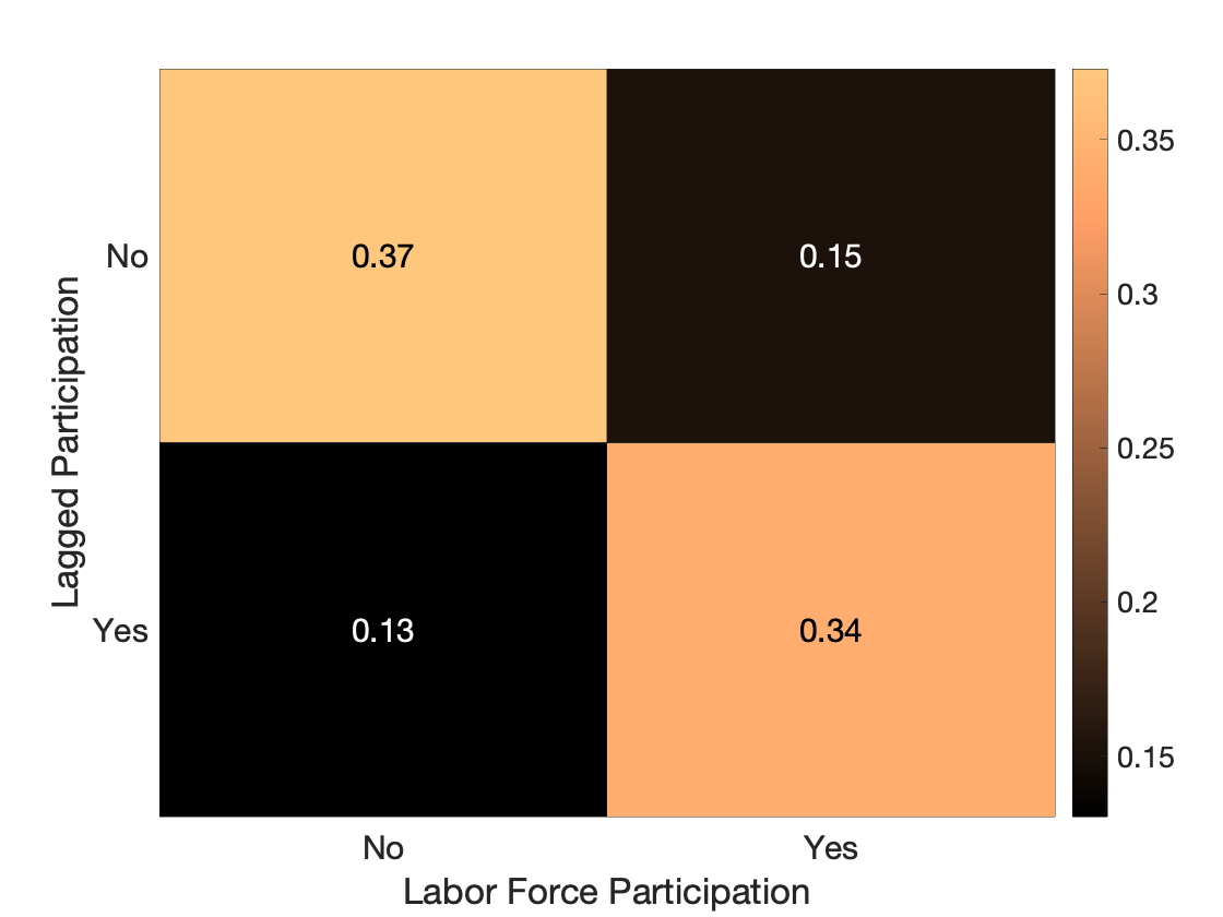
Figure H.1: Labor force participation contingency table. Each cell contains the percentage of individuals with given current and past LFP status.

[c]

Estimation results: Model (5.2)

	$\widehat{\theta}$	$\widetilde{\theta}$	$\text{Wald}_{\widehat{\theta}}$	$\text{Wald}_{\widetilde{\theta}}$	$\text{LM}_{\widehat{\theta}}$	$\text{LM}_{\widetilde{\theta}}$	$\text{LR}_{\widehat{\theta}}$	$\text{LR}_{\widetilde{\theta}}$
$\rho$	0.406	0.583	12.738	30.888	12.782	32.466	12.655	31.626
	(0.114)	(0.105)
$\lambda$	0.124	0.074	2.285	1.072	2.286	0.855	2.298	0.839
	(0.082)	(0.072)
$\beta_{1}$	-0.506	-0.503	8.031	10.075	8.053	9.704	8.153	9.746
	(0.178)	(0.159)
$\beta_{2}$	-0.364	-0.354	0.531	0.624	0.533	0.619	0.524	0.555
	(0.499)	(0.448)

• Notes: Standard errors in parentheses. The Wald, the LM and the LR statistics have limiting chi-squared distributions under $H_{0}$, with critical values given by $\chi^{2}\left(1\right)_{.99}=6.635,\chi^{2}\left(1\right)_{.95}=3.841,\chi^{2}\left(1\right)_{.90}=2.706$.

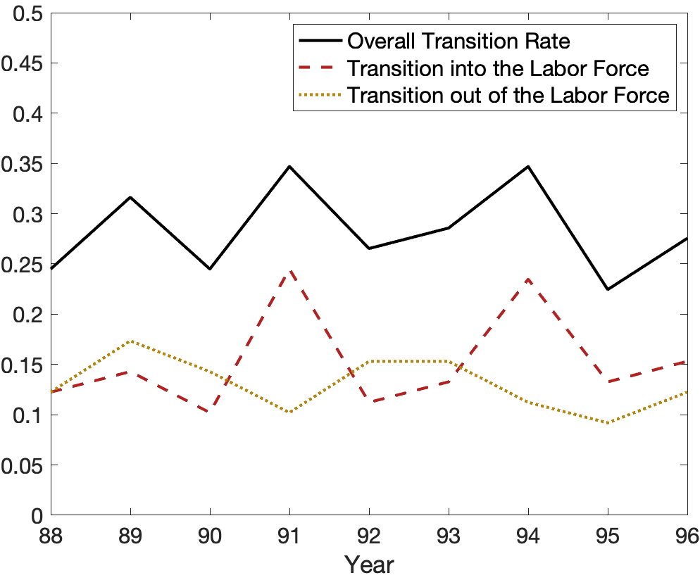
Figure H.2: Labor force participation status transition rates by year

[c]

Summary statistics: Heterogeneous labor supply elasticities with respect to the number of children based on model (5.2) estimates

				10th	25th	75th	90th
	Mean	Median	Std. Dev.	Percentile	Percentile	Percentile	Percentile
$\widehat{\lambda}_{it}$	0.124	0.099	0.524	-0.523	-0.262	0.483	0.808
$\widetilde{\lambda}_{it}$	0.074	0.054	0.457	-0.489	-0.254	0.383	0.670

• Notes: Standard errors in parentheses. The Wald, the LM and the LR statistics have limiting chi-squared distributions under $H_{0}$, with critical values given by $\chi^{2}\left(1\right)_{.99}=6.635,\chi^{2}\left(1\right)_{.95}=3.841,\chi^{2}\left(1\right)_{.90}=2.706$.

References

- Aguero and Marks (2008) Aguero, J. M. and M. S. Marks (2008, May). Motherhood and Female Labor Force Participation: Evidence from Infertility Shocks. American Economic Review 98(2), 500–504.
- Andersen (1970) Andersen, E. B. (1970). Asymptotic properties of conditional maximum-likelihood estimators. Journal of the Royal Statistical Society. Series B (Methodological) 32(2), 283–301.
- Angrist and Evans (1998) Angrist, J. D. and W. N. Evans (1998). Children and Their Parents’ Labor Supply: Evidence from Exogenous Variation in Family Size. The American Economic Review 88(3), 450–477. Publisher: American Economic Association.
- Arellano and Bond (1991) Arellano, M. and S. Bond (1991). Some tests of specification for panel data: Monte carlo evidence and an application to employment equations. The review of economic studies 58(2), 277–297.
- Arellano and Bonhomme (2009) Arellano, M. and S. Bonhomme (2009). Robust priors in nonlinear panel data models. Econometrica 77(2), 489–536.
- Arellano and Hahn (2016) Arellano, M. and J. Hahn (2016). A likelihood-based approximate solution to the incidental parameter problem in dynamic nonlinear models with multiple effects. Global Economic Review 45(3), 251–274.
- Bai (2009) Bai, J. (2009). Panel data models with interactive fixed effects. Econometrica 77(4), 1229–1279.
- Bai (2013) Bai, J. (2013). Fixed-effects dynamic panel models, a factor analytical method. Econometrica 81(1), 285–314.
- Bellio et al. (2023) Bellio, R., I. Kosmidis, A. Salvan, and N. Sartori (2023). Parametric bootstrap inference for stratified models with high-dimensional nuisance specifications. Statistica Sinica 33(2), 1–23.
- Blau and Kahn (2007) Blau, F. D. and L. M. Kahn (2007, July). Changes in the Labor Supply Behavior of Married Women: 1980-2000. Journal of Labor Economics 25(3), 393–438. Publisher: The University of Chicago Press.
- Blundell et al. (2016) Blundell, R., M. Costa Dias, C. Meghir, and J. Shaw (2016). Female Labor Supply, Human Capital, and Welfare Reform. Econometrica 84(5), 1705–1753.
- Chamberlain (1980) Chamberlain, G. (1980). Analysis of covariance with qualitative data. The Review of Economic Studies 47(1), 225–238.
- Charbonneau (2017) Charbonneau, K. B. (2017). Multiple fixed effects in binary response panel data models. The Econometrics Journal 20(3), S1–S13.
- Chen et al. (2021) Chen, M., I. Fernández-Val, and M. Weidner (2021). Nonlinear factor models for network and panel data. Journal of Econometrics 220(2), 296–324.
- Chernozhukov et al. (2013) Chernozhukov, V., I. Fernández-Val, J. Hahn, and W. Newey (2013). Average and quantile effects in nonseparable panel models. Econometrica 81(2), 535–580.
- Connelly (1992) Connelly, R. (1992). The Effect of Child Care Costs on Married Women’s Labor Force Participation. The Review of Economics and Statistics 74(1), 83–90. Publisher: The MIT Press.
- Cox and Snell (1968) Cox, D. R. and E. J. Snell (1968). A general definition of residuals. Journal of the Royal Statistical Society. Series B (Methodological) 30(2), 248–275.
- De Bin et al. (2015) De Bin, R., N. Sartori, T. A. Severini, et al. (2015). Integrated likelihoods in models with stratum nuisance parameters. Electronic Journal of Statistics 9(1), 1474–1491.
- Dhaene and Jochmans (2015a) Dhaene, G. and K. Jochmans (2015a). Profile-score adjustments for incidental-parameter problems.
- Dhaene and Jochmans (2015b) Dhaene, G. and K. Jochmans (2015b). Split-panel jackknife estimation of fixed-effect models. The Review of Economic Studies 82(3), 991–1030.
- Dhaene and Sun (2021) Dhaene, G. and Y. Sun (2021). Second-order corrected likelihood for nonlinear panel models with fixed effects. Journal of Econometrics 220(2), 227–252. Annals Issue: Celebrating 40 Years of Panel Data Analysis: Past, Present and Future.
- Eckstein and Lifshitz (2011) Eckstein, Z. and O. Lifshitz (2011). Dynamic Female Labor Supply. Econometrica 79(6), 1675–1726.
- Fan and Yao (2003) Fan, J. and Q. Yao (2003). Nonlinear time series: nonparametric and parametric methods. Springer Science & Business Media.
- Fernandez (2013) Fernandez, R. (2013). Cultural change as learning: The evolution of female labor force participation over a century. American Economic Review 103(1), 472–500.