Programming-by-Demonstration for Long-Horizon Robot Tasks (Extended Version)
Abstract.
Abstract. The goal of programmatic Learning from Demonstration (LfD) is to learn a policy in a programming language that can be used to control a robot’s behavior from a set of user demonstrations. This paper presents a new programmatic LfD algorithm that targets long-horizon robot tasks which require synthesizing programs with complex control flow structures, including nested loops with multiple conditionals. Our proposed method first learns a program sketch that captures the target program’s control flow and then completes this sketch using an LLM-guided search procedure that incorporates a novel technique for proving unrealizability of programming-by-demonstration problems. We have implemented our approach in a new tool called prolex and present the results of a comprehensive experimental evaluation on 120 benchmarks involving complex tasks and environments. We show that, given a 120 second time limit, prolex can find a program consistent with the demonstrations in 80% of the cases. Furthermore, for 81% of the tasks for which a solution is returned, prolex is able to find the ground truth program with just one demonstration. In comparison, CVC5, a syntax-guided synthesis tool, is only able to solve 25% of the cases even when given the ground truth program sketch, and an LLM-based approach, GPT-Synth, is unable to solve any of the tasks due to the environment complexity.
1. Introduction
Learning From Demonstration (LfD) is an attractive paradigm for teaching robots how to perform novel tasks in end-user environments (Argall et al., 2009). While most classical approaches to LfD are based on black-box behavior cloning (Ly and Akhloufi, 2021; Ho and Ermon, 2016), recent work has argued for treating LfD as a program synthesis problem (Holtz et al., 2020a; Xin et al., 2023; Porfirio et al., 2023). In particular, programmatic LfD represents the space of robot policies in a domain-specific language (DSL) and learns a program that is consistent with the user’s demonstrations.
Although this programmatic approach has been shown to offer several advantages over black-box behavior cloning in terms of data efficiency, generalizability, and interpretability (Holtz et al., 2021; Lipton, 2018), existing work in this space suffers from three key shortcomings: First, most prior techniques focus on simple Markovian policies that select the next action based only on the current state. As a result, the target programs have a simple decision-list structure, and the main difficulty lies in inferring suitable predicates for each branch. Second, most existing techniques have only been applied to restricted domains with limited object and interaction types, such as robot soccer playing where the entities of interest are known a priori and comprise a small set.
Our goal in this work is to develop a programmatic LfD approach for long-horizon tasks that commonly arise in service mobile robot settings — e.g., putting away groceries in a domestic setting, or proactively providing tools and parts to a mechanic in assistive manufacturing. Long-horizon robotics tasks are inherently more challenging, as the robot needs to reason about the interactions between a long sequence of actions (e.g., that the dishes must be cleared from a table before it can be wiped down) and the effect of specific environmental states on sequences of actions (e.g., a robot tasked with dusting a shelf must first remove all items from the shelf if it is not empty vs. directly dusting it if there are no items on it). This is in stark contrast to control tasks, such as motion control, where the policy just needs to select the next action for a single time step.
Recognizing the importance of long horizon tasks, recent work (Porfirio et al., 2023) has proposed a multi-modal user interface (combining natural language with hand-drawn navigation paths) to facilitate programmatic LfD in this setting. This paper makes another stride towards that goal, but in an orthogonal direction, by learning more complex programs from demonstration traces. In particular, the approach that we propose in this paper aims to (a) handle tasks that require complex control flow (such as nested loops with multiple conditionals) and (b) scale to demonstrations performed in complex environments with hundreds of objects and a large number of relationships to consider between those objects.
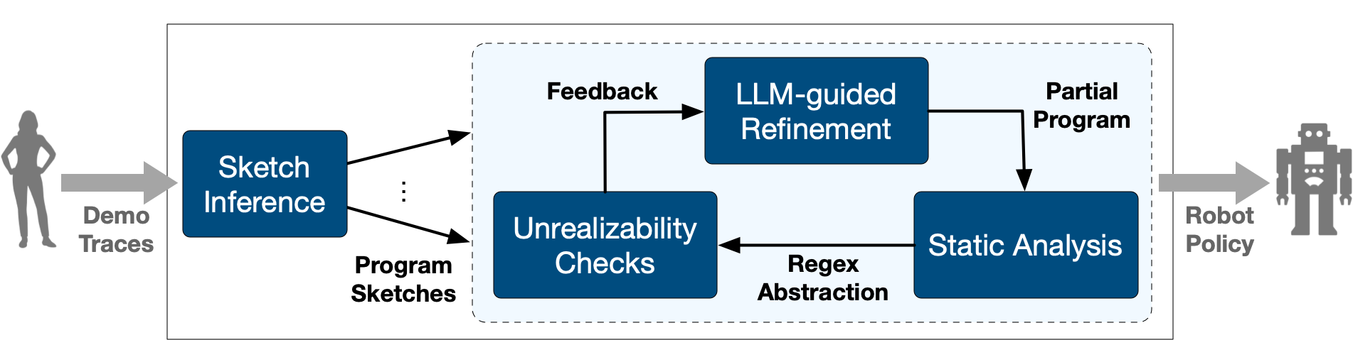
Our proposed approach tackles these two challenges using a novel program synthesis algorithm that is illustrated schematically in Figure 1. First, given a set of demonstration traces, our approach infers a control flow sketch of the target program. To do so, our method abstracts each demo trace as a string over a finite alphabet and then learns a set of simple regular expressions that “unify” all of the demonstrations. As there is an obvious correspondence between regex operators and control flow structures (e.g., loops as Kleene star; conditionals as disjunction), our method can quickly infer the control flow structure of the target program from a small number of demonstrations. Furthermore, because the sketch learner prefers small regular expressions over complex ones, this application of the Occam’s razor principle introduces inductive bias towards control structures that are more likely to generalize to unseen traces.
Given a program sketch capturing the underlying control flow structure, the second sketch completion phase of our algorithm tries to find a complete program that is consistent with the given traces. This algorithm is based on top-down enumerative search, meaning that it starts by considering all DSL programs as part of the search space and gradually refines it until it contains a single program. However, because the size of the search space is exponential with respect to the number of entities in the environment, such a search strategy does not scale to complex environments. Our approach deals with this challenge using two key ideas, namely (1) guiding the search procedure using a large language model (LLM), and (2) proving unrealizability of synthesis sub-problems.
LLM-guided refinement. As shown in Figure 1 (and as standard in the literature), our sketch completion procedure represents the search space as a partial program (i.e., a program containing holes), so the refinement step involves filling one of the holes in this partial program with a concrete expression. In our setting, these holes need to be instantiated with objects (or object types) in the environment, as well as properties of –and relationships between– those objects. However, because the demonstration may be performed in complex environments with many such objects and properties, each hole typically has a very large number of possible completions. To address this problem, our method consults an LLM to perform refinement; intuitively, this serves two purposes: First, when the target program contains object types that do not explicitly occur in the demonstrations (a very common scenario), LLM guidance allows the synthesizer to propose new entities by reasoning about commonalities between objects that do occur in the demonstrations. Second, by conditioning the current prediction on previous ones, the synthesizer can avoid generating programs that do not “make sense” from a semantic perspective.
Proving unrealizability. However, even with LLM guidance, the search procedure may end up constructing partial programs that have no valid completion with respect to the demonstrations. Our approach tries to avoid such dead-ends in the search space through a novel procedure for proving unrealizability. In particular, given a partial program , our approach performs static analysis to construct a suitable abstraction, in the form of a regex, that represents all possible traces of all completions of for the demonstration environment. Given such a regex , proving unrealizability of a synthesis problem boils down to proving that the demonstration trace cannot possibly belong to the language of .
We have implemented the proposed LfD technique in a tool called prolex111Programming RObots with Language models and regular EXpressions and evaluate it on a benchmark set containing 120 long-horizon robotics tasks involving household activities. Given a 2 minute time limit, our approach can complete 80% of the synthesis tasks and can handle tasks that require multiple loops with several conditionals as well as environments with up to thousands of objects and dozens of object types. Furthermore, for 81% learning tasks that prolex is able to complete within the 2 minute time limit, prolex learns a program that matches the ground truth from just a single demonstration. To put these results in context, we compare our approach against two relevant baselines, including CVC5, a state-of-the-art SyGuS solver and GPT-Synth, a neural program synthesizer, and experimentally demonstrate the advantages of our approach over other alternatives. CVC5 is only able to solve 25% of the tasks even when given the ground-truth sketch. GPT-Synth, on the other hand, is unable to solve any of the tasks due to environment complexity, even when the environment is simplified to include only a small fraction of the objects in addition to the required ground truth entities. Furthermore, we report the results of a series of ablation studies and show that our proposed ideas contribute to successful synthesis.
In summary, this paper makes the following contributions:
-
•
We propose a novel programming-by-demonstration (PBD) technique targeting long-horizon robot tasks. Our approach can learn programs with complex control flow structures, including nested loops with conditionals, from a small number of traces and in complex environments with thousands of objects.
-
•
We propose a new (reusable) method for proving unrealizability of synthesis problems in the PBD setting.
-
•
We implement these ideas in a tool called prolex and evaluate its efficacy in the context of 120 benchmarks involving 40 unique household chores in three environments. prolex can complete the synthesis task within 2 minutes for 80% of the benchmarks, and, for 81% of the completed tasks, prolex is able to learn the ground truth program from just a single demonstration.
2. Motivating Example
In this section, we present a motivating example to illustrate our programmatic LfD approach. Imagine a hotel worker who wants to instruct a robot to collect dirty sheets from guest rooms and place them in a laundry bin in the room. The goal of LfD is to teach this task through demonstrations rather than explicitly programming the robot. We formalize user demonstrations in a form that is amenable to be captured using smart hand-held devices, similar to existing end-user robots like the iRobot Roomba (iRobot, 2023) and Amazon Astro (Lee et al., 2023).
| Loc | State | |
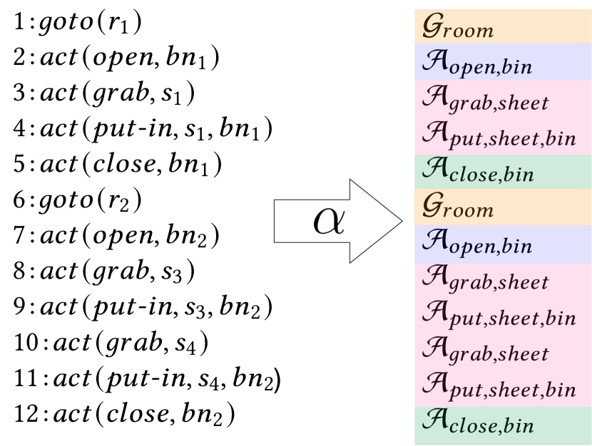
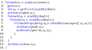
User Demonstration. For the above task, suppose that the hotel worker performs a demonstration consisting of the 12 actions shown in the left side of Figure 2(a). The demonstration takes place in two rooms, and ; Figure 3 shows the state of these two rooms before the demonstration takes place. Each room contains a large number of objects, including a bed, a laundry bin, and a few sheets on the bed. In particular, there is a clean sheet () and a dirty sheet () on the bed in , and there are two dirty sheets ( and ) on the bed in . Note that the complete representation of the rooms includes many more object types and properties, which are omitted from the figure due to space constraints. The first five steps of the demonstration sequence shown in Figure 2(a) (left) correspond to the actions performed in , and the remaining seven steps indicate the actions performed in . Specifically, indicates going to the location , and indicates performing a specific action on objects . Hence, in our example demonstration, the user first visits room , where they open bin , grab and place sheet in that bin, and finally close the bin. Next, they go to the second room, , and repeat a similar sequence of actions with the bin , and sheets and .
Desired Output. Since our goal is to perform programmatic LfD, we wish to learn a programmatic robot execution policy from the provided demonstration. Figure 2(d) shows the desired policy that generalizes from the user’s only demonstration. Intuitively, this policy encodes that the robot should go to each room (line 2), identify a bin and all beds present in that room, collect all dirty sheets from the top of each bed (lines 7-8), and place them in the bin (line 9). The program also contains perception primitives that enable the robot to become aware of its environment (lines 1, 3, 5, and 6). In particular, the function allows the robot to identify all objects of type that are visible from its current location and reason about their properties and relations. Function is similar but returns all locations of type . Synthesis of appropriate perception primitives is crucial for effective LfD, since the robot must be able to observe and reason about the state of objects in new and unseen environments.
Synthesis Challenges. In this context, generating the desired policy from the user’s demonstration is challenging for several reasons: (1) the desired program has complex control flow, with three nested loops and an if statement with multiple predicates, (2) the desired program requires performing appropriate perception actions that have no correspondence in the given demonstrations, and (3) the desired program requires reasoning about high-level concepts that are also not indicated in the demonstrations, such as being dirty or being on top of some other object. Additionally, observe that the synthesized program needs to refer to object types (e.g., bed) that are not involved in the demonstration. Hence, the synthesizer cannot only consider those objects in the demonstration, as the desired program could refer to any of the entities in the environment. This means that the difficulty of the synthesis task is inherently sensitive to the complexity of the environment.
Our Approach. Our algorithm first generates a set of sketches of the target program based on the demonstration. These sketches capture the control flow structure of the target program but contain many missing expressions (“holes”). The goal of the subsequent sketch completion step is to fill these holes in a way that scales to complex environments.
Sketch generation. To generate a sketch, our method first abstracts the user’s demonstrations as a set of strings: Figure 2(a) (right) shows the string abstracted from the user’s sole demonstration using an abstraction function , where and denote and in the demonstration, and the subscripts indicate the type of their arguments. For example, even though the demonstration specifies that the user grabbed specific sheets (namely, , , and ), the string abstraction omits such details and represents all three instances of this action using . Each character in the abstract string is highlighted using a different color to visually aid the reader. The idea of converting the demonstration to a more abstract form is a crucial first step towards generalization.
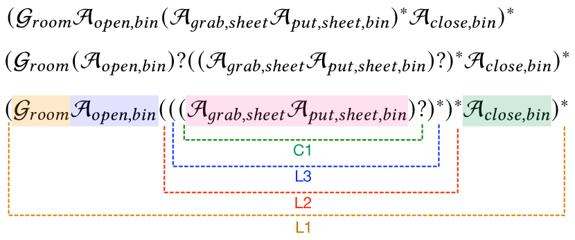
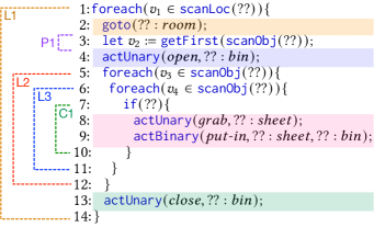
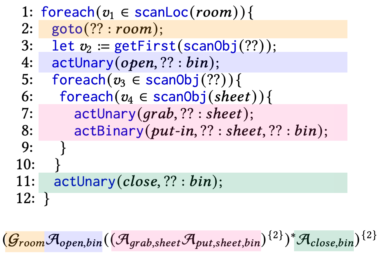
Next, our approach utilizes existing techniques to synthesize a regex that matches the string encoding of the demonstrations: Figure 2(b) presents three regular expressions that all match the string abstraction of the given demonstration. Note that there is an obvious parallel between regex operators and the program’s control flow: Since Kleene star denotes repetition, it naturally corresponds to a looping construct. Similarly, since the optional operator (i.e., ) denotes choice, it is naturally translated into an statement. Thus, given a candidate regex for the demonstrations, our approach translates it into a sketch in a syntax-directed way. For instance, the third regular expression from Figure 2(b) is translated to the sketch shown in Figure 2(c), where the three nested loops and the conditional block are marked using the same colored dashed lines both in the regex and in the sketch. Additionally, because the program should not manipulate any objects before it perceives them, our sketch generation procedure also inserts any necessary perception primitives to the sketch. For instance, the sketch in Figure 2(c) contains an inferred let binding (labelled ), since the object of type at line 4 cannot be acted upon before it is first perceived by the robot.
Sketch completion. For each sketch generated in the first step, our method tries to find a completion that matches the user’s demonstration. In practice, several of these sketches are unrealizable, meaning that there is no completion that will match the user’s demonstrations. For example, consider the first regex presented above in Figure 2(b) that matches the string abstraction of the demonstration. This regex does not include the optional operator used in the correct regex. Intuitively, sketches generated from this regex will be infeasible because, without an if statement in the sketch, the resulting programs would end up grabbing both sheets in room , rather than only the single dirty sheet. Hence, the second phase of our technique considers multiple sketches and tries to find a completion of any sketch that is consistent with the given demonstrations.
Our sketch completion algorithm is based on top-down enumerative search but (a) utilizes a novel unrealizability checking procedure to quickly detect dead-ends and (b) leverages an LLM to guide exploration. In particular, starting from a sketch, the synthesis algorithm maintains a worklist of partial programs containing holes to be filled. When dequeuing a partial program from the worklist, we consider its probability according to the LLM, so more promising partial programs are prioritized over less likely ones. Going back to our example, consider a partial program where we test the color of a bedsheet before putting it in the bin. Because the concepts “laundry bin” and “cleanliness” are much more related compared to “color” and “laundry bin”, our technique prioritizes a program that includes the conditional over one that is based on color.
Our sketch completion method also leverages the demonstration to prove unrealizability of a given synthesis problem. As an example, consider the partial program shown in Figure 4. We can prove that there is no completion of this partial program that will be consistent with the user’s demonstrations: Because none of the actions in the partial program modify object locations and because there are two sheets in each room, any completion of this partial program would end up performing the action at least four times but there are only three actions in the trace. Hence, this partial program is a dead end, and our approach can detect unrealizability of such a synthesis sub-problem. To do so, it statically analyzes the partial program to infer upper and lower bounds on the number of loop executions. It then uses this information to construct a regex, shown at the bottom of Figure 4, that summarizes all possible traces that this partial program can generate. Since the demo trace from Figure 2(a) is not accepted by the regular expression in Figure 4, our algorithm can prove the unrealizability of this synthesis problem.
3. Robot Execution Policies
In this section, we introduce a domain-specific language (DSL) for programming robots and provide a formal definition of the robot learning from demonstrations (LfD) problem.
3.1. Syntax
The syntax of the our DSL is presented in Figure 5. A robot program () contains functions to perform various operations on a single object () or a pair of objects (). The robot can move between locations using the function. The robot becomes aware of its location by scanning the environment using , and it becomes aware of objects in its current location using the function. The result of running a scan operation is an ordered list of location or object instances (denoted by ) of the specified type . For example, yields all plates at the current location of the robots. Specific elements in the scan result can be bound to variables using a restricted let binding of the form . This expression introduces a new variable and assigns the ’th element of list to . As standard, the DSL also contains typical conditional and looping control structures. Conditional expressions check properties of objects (), relationships between them (), as well as their Boolean compositions. The abstractions for robot actions and perception in our DSL is similar to widely used accepted symbolic abstractions for classical planning (Aeronautiques et al., 1998; Fox and Long, 2003), and more recently, symbolic robot policies (Liang et al., 2022).
Note that the DSL presented in Figure 5 is parametrized over a set of domain-specific terminals, indicated by an asterisk. For example, location types are not fixed and can vary based on the target application domain. For example, for robot execution policies targeting household chores, locations might be kitchen, living room, basement etc. Similarly, object types, properties, relations, and actions are also domain-specific and can be customized for a given family of tasks.
3.2. Operational Semantics
In this section, we present the operational semantics of our robot DSL using the small-step reduction relation shown in Figure 6. This relation formalizes how the robot interacts with its environment while executing the program. Specifically, the relation is defined between tuples of the form , where is a program, is the robot’s execution environment, is a valuation (mapping variables to their values), and is a program trace. In more detail, the environment is a quadruple where is a set of typed location identifiers; is a mapping from (typed) object identifiers to their corresponding location; is the current location of the robot; and is an interpretation for all the relation symbols. That is, for a relation , yields the set of tuples of objects for which evaluates to true. Given object type and a location , we write to denote the list of all objects that are at location and that have type . Similarly, given a location type , the list of locations of this type is denoted by . Finally, a trace is a sequence of actions performed by the robot. Robot actions are denoted using and , where is an action that was performed on objects , and is a location that the robot visited. Note that robot execution policies are effectful programs: for example, the location of the robot or some properties of an object can change after executing .
(sequence)
(skip)
(if-t)
(if-f)
(act-unary)
(act-binary)
(goto)
(let-obj)
(foreach-obj)
(let-loc)
(foreach-loc)
With the above notations in place, we now explain the operational semantics from Figure 6 in more detail. The first rule, labeled (sequence), defines how the robot takes a step by executing the first statement in the program. The next rule (skip) defines the semantics of executing a statement, which has no effect on the execution state. The rules (if-t) and (if-f) describe the flow of the program when a conditional statement is executed. First, the Boolean expression is evaluated to or , depending on the result, the program either skips or executes . Boolean expressions are evaluated using the relation defined in Figure 7. This relation is parameterized by the execution environment and valuation .
(check_prop_t)
(check_prop_f)
(check_rel_t)
(check_rel_f)
(negation)
(conjunction)
(disjunction)
The (act-unary) and (act-binary) rules specify the outcomes of executing a unary and a binary action, respectively, using the auxiliary relation . Given an environment , an action and affected object instance(s), the relation formalizes how the environment is modified based on the semantics of action . Since our DSL is parameterized over the set of actions, we do not discuss the relation in detail in the main body of the paper and refer the interested reader to Appendix A.1 for a representative subset of actions used in our evaluation.
The goto rule defines the effect of executing a statement, where the environment is updated to reflect the robot’s new location, and a new trace element is generated and appended to the existing trace, where is the location stored in variable . Next, the rules let-obj and let-loc, define the semantics of the statement, which assigns to variable the element of list obtained via either or . Specifically, yields all objects of type that are present at the robot’s current location, and yields all locations of type . The rules (foreach-obj) and (foreach-loc) describe the semantics of loops of the form , where is the result of a scan operation. As expected, these rules iteratively bind to each of the elements in and execute the loop body under this new valuation.
Finally, we use the relation to define the semantics of executing a policy on environment . Given and robot execution policy , we write iff where denotes an empty list/mapping.
3.3. Problem Statement
In this section, we formally define the LfD problem that we address in this paper. Informally, given a set of demonstrations , the LfD problem is to find a robot execution policy (in the DSL of Figure 5) such that is consistent with . To make the notion of consistency more precise, we represent a demonstration as a pair where is the initial environment and is a trace of the user’s demonstration in this environment.
Definition 3.1.
(Consistency with demonstration) We say that a robot execution policy is consistent with a demonstration , denoted , iff .
We also extend this notion of consistency to a set of demonstrations , and we write iff for every demonstration in . We can now formalize our problem statement as follows:
Definition 3.2.
(Programmatic LfD) Given a set of demonstrations , the programmatic LfD problem is to find a robot execution policy such that .
4. Synthesis Algorithm
In this section, we present our synthesis technique for solving the programmatic LfD problem defined in the previous section. We start by giving an overview of the top-level algorithm and then describe each of its key components in more detail.
4.1. Top-Level Algorithm
Our top-level learning procedure is presented in Algorithm 1. This algorithm takes as input a set of demonstrations and returns a policy such that for all , we have . If there is no programmatic policy that is consistent with all demonstrations, the algorithm returns .
The synthesis procedure starts by constructing an abstraction of each demonstration as a string over the alphabet where indicate location and object types (e.g., , ) and denotes a specific type of action (e.g., ). This abstraction is performed at line 2 of Algorithm 1 using the function , defined as follows:
where denote the type of location and object respectively. In other words, when abstracting a trace as a string, the algorithm replaces specific object instances with their corresponding types. Intuitively, this abstraction captures the commonality between different actions in the trace, allowing generalization from a specific sequence of actions to a more general program structure.
Next, given the string abstraction of the demonstrations , the loop in lines 3–12 alternates between the following key steps:
-
•
Regex synthesis: The GetNextRegex procedure at line 4 finds a regular expression matching all strings in . Intuitively, this regex captures the main control flow structure of the target program and can be used to generate a set of program sketches.
-
•
Sketch generation: The inner loop in lines 6–10 translates a given regex to a set of program sketches. As shown in Figure 8, a sketch has almost the same syntax as programs in our DSL except that the arguments of most constructs are unknown, as indicated by question marks. In particular, note that (1) the types of objects and locations being scanned are unknown, (2) predicates of statements are yet to be determined, and (3) the specific objects and locations being acted on are also unknown (although their types are known).
-
•
Sketch completion: Given a candidate program sketch , line 9 of the algorithm invokes CompleteSketch to find a completion of that is consistent with the demonstrations. If CompleteSketch does not return failure (), the synthesized policy is guaranteed to satisfy all demonstrations; hence, Synthesize returns as a solution at line 10.
In the remainder of this section, we describe sketch generation and sketch completion in more detail. Because learning regexes from a set of positive string examples is a well-understood problem, we do not describe it in this paper, and our implementation uses an off-the-shelf tool customized to our needs via some post-processing (see Section 5).
4.2. Sketch Inference
Given a regex over the alphabet , the goal of sketch inference is to (lazily) generate a set of program sketches. The inputs to the sketch inference procedure are regular expression of the following form:
Given such a regex, sketch inference consists of two steps:
-
(1)
Syntax-directed translation: In the first step, sketch inference converts the given regex to control flow operations using syntax-directed translation. Intuitively, string concatenation is translated into to sequential composition; Kleene star corresponds to loops; and, optional regexes translate into conditionals.
-
(2)
Perception inference: While the sketches generated in step (1) are syntactically valid, they may lack essential perception operations (i.e., and ). Hence, in the second step, our sketch inference procedure inserts these perception operations such that the resulting sketch is perception-complete, meaning that it contains at least the minimum number of required scan operation. However, since the target program may require additional operations, the second step of sketch inference yields a set of sketches that only differ with respect to the placement of these perception operations.
Figure 9 presents our syntax-directed translation rules for converting regular expressions to a syntactically valid sketch using judgments of the form , meaning that regex is translated to sketch . As expected, characters are translated to , , and constructs respectively. The Kleene star operator is translated into a looping construct, but may iterate either over locations or objects. Finally, regex concatanation is translated into sequential composition, and is translated into a conditional with an unknown predicate.
Recall that our DSL also allows bindings that assign a new variable to the result of a perception operation. Since program traces (and, hence, the inferred regexes) do not contain these perception operations, the last two rules in Figure 9 allow inserting bindings at arbitrary positions in the sketch. In particular, if can be translated into a sketch , then the last two rules of Figure 9 state that can also be translated into a sketch of the form where is a new binding which assigns a fresh variable to an entity that is obtained by scanning objects or locations.
In general, observe that a regex can give rise to a large number of program sketches, as we do not a priori know where to insert bindings. To tackle this problem, our lazy sketch inference procedure first translates a regex into a sketch without using the last two rules in Figure 9 for inserting bindings. In a second step, it infers where perception operations are needed and inserts let bindings according to the results of this analysis.
This second step of our sketch inference procedure is formalized using the notion of perception completeness. Intuitively, a sketch is perception complete if the program perceives (using operations) all objects that it manipulates, before it manipulates them. If a sketch is not perception complete, it can never be realized into a valid program; hence, it is wasteful to consider such sketches. We formalize the notion of perception completeness using the following definition:
Definition 4.1.
(Perception Completeness) Let denote a standard partial order between program points.222We refer the interested reader to the chapter 6 of ”Programming Language Pragmatics” by Michael L. Scott (2000) for a detailed discussion on program orders and their usage in control flow analysis. A sketch is said to be perception complete if the following conditions are satisfied:
-
(1)
for all in , there exists a such that .
-
(2)
for all in , there exist and , such that and .
-
(3)
for all in , there exists a statement in such that .
Our sketch inference algorithm leverages this notion of perception completeness to lazily enumerate program sketches as follows: First, it translates a given regex into a set of sketches using the inference rules shown in Figure 9 but without using the last two rules. It then infers a minimal set of applications of the last two rules needed to make the sketch perception complete and then augments the resulting sketches with the inferred bindings. Finally, because additional bindings may be needed, it lazily inserts more bindings (up to a bound) if the current sketch does not produce a valid completion.
4.3. Sketch Completion
We now turn our attention to the sketch completion procedure, shown in Algorithm 2, for finding a sketch instantiation that satisfies the given demonstrations. Given a sketch and demonstrations , CompleteSketch either returns to indicate failure in finding a policy that is consistent with all demonstrations. Note that the sketch completion procedure is parameterized over a statistical model for assigning probabilities to possible sketch completions.
CompleteSketch is a standard top-down search procedure that iteratively expands partial programs until a solution is found.333Partial programs belong to the grammar from Figure 5 augmented with productions for each non-terminal . However, our sketch completion procedure has two novel aspects: First, it assigns probabilities to partial programs using a large language model, and second, it uses a novel compatibility checking procedure for proving unrealizability of synthesis problems.
In more detail, the sketch completion procedure initializes the worklist to a singleton containing the input sketch , with corresponding probability (line 2). It then enters a loop (lines 3–14) where each iteration processes the highest probability partial program in the worklist. If the dequeued partial program is complete, meaning that it has no holes (line 5), the algorithm checks whether all demonstrations are satisfied (line 6). If so, is returned as a solution; otherwise, it is discarded. If is incomplete, the algorithm performs a compatibility check at line 8 to avoid solving an unrealizable synthesis problem. Next, if is a compatible with the demonstrations, the algorithm considers one of the holes in and all well-typed grammar productions that can be used to fill that hole. In particular, given a hole , the procedure Fill yields a set of expressions such that (1) is a production in the grammar, and (2) replacing with can result in a well-typed program. Hence, for each such expression , we obtain a new partial program at line 11 by replacing hole in with expressions .444When doing the replacement , all non-terminals occurring in are replaced with a hole . However, since some completions are much more likely than others, our algorithm assigns probabilities to completions using the statistical model . Hence, when dequeuing partial programs from the worklist, the algorithm prioritizes programs that are assigned a higher probability.
4.3.1. Proving Unrealizability
A key component of our sketch completion procedure is a novel technique for proving unrealizability of a programming-by-demonstration (PbD) problem. While there has been significant prior work on proving unrealizability in the context of programming-by-example (PbE) (Hu et al., 2019; Kim et al., 2023; Feng et al., 2018a), such techniques only consider the input-output behavior rather than the entire execution trace. In contrast, our goal is to prove unrealizability of synthesis problems where the specification is a set of demonstrations (i.e., traces).
Given a partial program (representing a hypothesis space), our key idea is to generate a regex such that the language of includes all possible traces of all programs in the hypothesis space. Hence, if there exists some trace where is not accepted by , this constitutes a proof that the synthesis problem is unrealizable.
Our algorithm for checking compatibility between partial programs and traces is presented in Algorithm 3. At a high level, this algorithm iterates over all demonstrations (lines 2–5) and returns false if it can prove that is incompatible with some demonstration in . To check compatibility with , the algorithm first partially evaluates on the initial environment to obtain a simplified program , as done in existing work (Feng et al., 2017). The novel part of our technique lies in constructing a regex abstraction of the partial program under a given environment . Specifically, our compatibility checking procedure constructs a regex that over-approximates the possible behaviors of under initial environment . In particular, the regex is constructed at line 4 in such a way that if is not accepted by , then no completion of can be compatible with (see, Theorem 4.2).
Hence, the crux of the compatibility checking algorithm is the ProgToRegex procedure (formalized as inference rules shown in Figures 10 and 11) for generating a regex that over-approximates the behavior of under environment . These rules utilize the notion of an abstract environment which is a triple where (1) CurLoc is a set containing all possible locations that the robot could currently be at; (2) Locs is a mapping from location types to the set of locations of that type; (3) Objs is a mapping from each location to the set of objects of each type at that location (or if unknown). Because statements in our DSL can modify the environment, this notion of abstract environment is used to conservatively capture (the possibly unknown) side effects of partial programs on the environment. The inference rules shown in Figures 10 and 11 formalize the ProgToRegex procedure using two types of judgments:
-
(1)
Scan rules (shown in Figure 10) are of the form , indicating that the cardinality of the set returned by must be some element of . For example, if , this means that the number of objects/locations returned by scan is either or . On the other hand, if includes the special element, then the number of elements is unknown.
-
(2)
Partial program rules (shown in Figure 11) are of the form , meaning that, under initial abstract environment , (a) the behavior of is over-approximated by regex , and (b) is a new environment that captures all possible environment states after executing on .
Before we explain these rules in detail, we first describe the high level idea, which is to encode (a) atomic actions using characters drawn from the alphabet , (b) statements using optional regexes, and (c) loops using regexes of the form where denotes the number of times the loop will execute (or as if the number of loop iterations is completely unknown). As mentioned in earlier sections (and, as we demonstrate empirically in Section 6), static reasoning about the number of loop iterations improves the effectiveness of our unrealizability checking procedure. With this intuition in mind, we now explain the rules shown in Figures 10 and 11.
Scan rules.
There are two sets of rules for scan operations, (loc-known) and (loc-unknown) for scanning locations, and (obj-known) and (obj-unknown) for scanning objects. For a operation, if its argument is a known location type , we simply look up the number of locations of that type from the given abstract environment. If it is unknown, we take the union over all possible location types. The rules for are similar: The (Obj-Known) rule handles the case where the argument is a known object type . In this case, we consider all the locations that the robot could be currently at and take the union of the number of objects of type for all of those locations. In the Obj-Unknown rule, we additionally take the union over all possible object types, since the argument of the operation is unknown.
Atomic actions.
The rule labeled (atomic) in Figure 11 deals with , and statements and serves two roles. First, it abstracts the performed action as a letter in our regex alphabet using the abstraction function . Second, it produces a new abstract environment by considering all possible effects of the action on the input environment via the UpdateAbsEnv function. Since the UpdateAbsEnv function is domain-specific and depends on the types of actions of interest, we do not describe in detail but provide a set of representative examples in Appendix A.4.
Sequence.
Sequential composition is abstracted using regex concatanation, and its final effect on the environment is captured by threading the environment through the two premises of the rule.
Conditionals.
As expected, if statements are abstracted using the optional operator (). Furthermore, since we do not know whether the predicate evaluates to true or not555Recall that we apply partial evaluation before performing this step. Hence, if the predicate of a conditional can be fully evaluated, it will be simplified away and rewritten as conditional-free code., we take the join of the two abstract environments. Intuitively, the join of abstract environments and , denoted by , is the smallest environment that over-approximates both and . An abstract environment is said to over-approximate an abstract environment , denoted by , if and only if:
Then, we can define a join operator on abstract environments as follows:
Intuitively, is the result of joining and if it is the smallest abstract environment that over-approximates both.
(loc-known)
(loc-unknown)
(obj-known)
(obj-unknown)
(atomic)
(seq)
(if)
(let)
(loop)
Loops.
The last rule in Figure 11 summarizes the analysis of loops. First, since the environment may be modified in the loop body, this rule first computes an inductive abstract environment, , for the loop (see Section 5 for further details). In particular, the premise ensures that over-approximates the initial environment, thereby establishing our base case. Second, the premise ensures that is preserved in all iterations of the loop body. Furthermore, because is an over-approximation of the environment that the loop body operates in, the regular expression also over-approximares the behavior of . Finally, to over-approximate the behavior of the entire loop, we determine the possible number of loop executions using the rules from Figure 10 under the initial environment . If can yield different objects, then the behavior of the loop is captured as . However, since we may not be able to compute the exact number of objects returned by a scan operation, we consider all possible cardinalities of the resulting set. Hence, the behavior of the loop is captured by the disjunction of the regexes .
The following theorem states that none of the completions of an unrealizable partial program is consistent with all demonstrations (see Appendix A.5 for the proof). An immediate corollary is the bounded completeness of our search algorithm, i.e., that Algorithm 1 always finds a program consistent with the demonstrations if it exists within the bounds of the search space.
Theorem 4.2.
Let be a partial program and let be a set of demonstrations. Then, for any complete program that is a completion of , we have:
4.3.2. Using LLM for Sketch Completion
We conclude this section with a discussion of how prolex infers a probability distribution over partial programs by prompting a large language model. Our prompting approach is inspired by the success of LLMs in addressing the “Fill in the Middle (FIM)” challenges in NLP literature (Liu et al., 2023). We reduce the sketch completion task to a FIM problem, as described below.
Given a partial program with a hole to fill, our approach encodes the context of in as a natural language prompt with unknown masks (Devlin et al., 2019). The prompt includes the set of valid completions for each mask, chosen by the procedure in Algorithm 2, to ensure the resulting program is well-typed. The LLM is then instructed to infer a probability distribution over the set of completions (represented by in Algorithm 2). This procedure is repeated whenever a partial program is expanded into a set of partial programs, to prioritize the enumerative search towards the intended program.
To illustrate how prolex prompts the LLM, Figure 12(a) (top) shows a partial program containing six unfilled holes, denoted as . Figure 12(b) (top) shows the prompt used for completing hole , which essentially corresponds to a natural description of the program.666Note that the demonstration is implicitly encoded as part of the partial program using type information for each hole. To generate such a prompt, our approach translates control-flow constructs to natural language in a syntax-directed way and replaces some of the holes ( and in this example) with masks. Because the remaining holes will be replaced with synthetic variable names like , they are not meaningful to the LLM; so our approach simply uses the types of these holes rather than masks when translating the partial program to natural language. As we can see from the LLM output in Figure 12(b), the highest likelihood completion of is deemed to be bed by the model, so the sketch completion algorithm prioritizes this completion over other alternatives such as chair or mug.
LLM Output for : {Bed: 0.8, Chair: 0.1, Mug: 0.05, …}
LLM Output for : {Dirty: 0.75, Folded: 0.2, White: 0.02, …}
LLM Output for : {On-top-of: 0.9, Under: 0.05, …}
As another example, consider the process of filling hole , and suppose that the algorithm has already refined to the conjunct as shown in the bottom part of Figure 12(a). When generating the prompt for , both holes and are filled with masks, and the LLM outputs dirty as the most likely completion for . When querying the remaining hole (), has already been filled with dirty, so the prompt only contains a single mask, and the LLM outputs on-top-of as the most likely completion. As illustrated by these examples, the LLM-guided search strategy allows the sketch completion engine to quickly home in on the right concepts (such as bed, dirty, and on-top-of in this example) and therefore allows the search procedure to focus on the most promising sketch completions.
5. Implementation
We implemented the proposed approach in a tool called prolex written in Python. In this section, we discuss salient aspects of prolex that are not covered in the technical sections.
Regex Learner. Our implementation leverages an open-source library to learn regular expressions from positive samples (Nordmann, 2014). However, since our sketch generation procedure does not allow arbitrary regex operators, our implementation post-processes the synthesized regexes by applying a set of rewrite rules. For instance, because our sketch generation procedure does not allow arbitrary disjunction, one of the rewrite rules () replaces disjunction with an optional operator. The full list of our rewrite rules can be found in Appendix A.3.
Large Language Model. Our sketch completion module utilizes the BERT large language model (Devlin et al., 2019), with pre-trained weights obtained from the HuggingFace library (Wolf et al., 2020). Since our algorithm generates masked language modeling (MLM) queries, we chose to use the bert-base-uncased model. This model is primarily fine-tuned for tasks that make use of the whole sentence, potentially with masked words, to make decisions. It is a lightweight model, and in our experiments, it consistently returns responses in less than on average.
Parallel Sketch Completion. The inherent independence of program sketches naturally lends itself to parallelization of the search process. To take advantage of this, prolex spawns a new process to execute sketch completion (Algorithm 2) for each generated sketch.
Computing Loop Invariants. Recall that our procedure for proving unrealizability relies on an inductive abstract environment for translating loops to regular expressions. Our implementation conservatively models the effect of any statement with holes by assuming that the hole could be filled with any value, and it performs standard least fixed point computation under these conservative semantics.
6. Evaluation
In this section, we present experiments designed to answer the following research questions:
-
(RQ1)
How effective is prolex at learning policies from human demonstrations?
-
(RQ2)
What is the relative significance of each of the key components in our synthesis algorithm?
-
(RQ3)
How does prolex compare against relevant baselines in terms of learning policies that match the user’s intention?
| Env | # Obj. | # Obj. | # Props. |
| Types | Instances | ||
| Easy | 40 | 140 | 609 |
| Medium | 60 | 295 | 2455 |
| Hard | 80 | 1109 | 13944 |
6.1. Benchmarks and Experimental Set-up
Tasks. We evaluate prolex on a set of 40 programmatic LfD problems involving long-horizon service tasks in typical household environments. We gathered these tasks from two sources, which we describe below.
First, we use 25 tasks from the Behavior Project (Srivastava et al., 2022). This project is an interactive platform designed for a virtual embodied AI agent operating within simulated household environments. The Behavior Project offers simulation videos of the agent carrying out a range of long-horizon tasks. These demonstrations are produced by human users who use a joystick to control the agent’s movements and actions in the simulation environment. Out of 100 tasks provided in the Behavior project, we observed that 75 required precise low-level motion control of the robot’s arms, like detailed cleaning of a car’s surfaces. As our DSL can trivially execute these tasks without any conditionals or loops, we excluded them from our evaluation. The demonstration videos for the remaining 25 tasks were transcribed using our action alphabet by an expert annotator —one of the authors— who is knowledgeable about the skill abstractions used by the robot.777Note that, in principle, this step could be performed by an off-the-shelf vision-to-action detection (V2A) algorithm (Ashutosh et al., 2023; Nazarczuk and Mikolajczyk, 2020). However, since this perception inference is orthogonal to our main problem, we opt to directly use the expert annotations.
Next, to broaden the scope of our evaluation and include more realistic tasks, we surveyed students at our institution and collected 15 additional tasks to evaluate prolex on. We did not impose any requirements regarding the users’ technical expertise, as our aim was to gather a list of household tasks that a typical end-user would consider beneficial to have automated
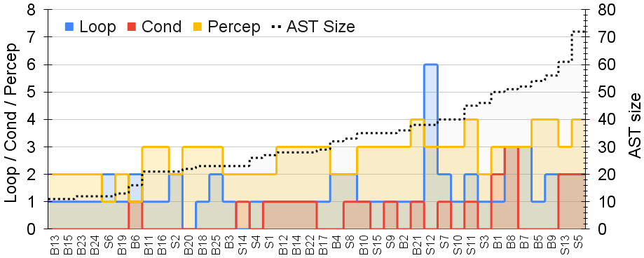
A full list of the above 40 tasks and their ground-truth programs is provided in Appendix A.6. Figure 13(a) presents an overview of the ground-truth programs for these tasks, ordered by program size. In more detail, the right y-axis represents program size (measured in terms of the number of nodes in the abstract syntax tree) and the left y-axis represents the number of loops, conditionals and perception primitives in the program. Tasks from the Behavior project are labeled as , and surveyed tasks are labeled as .
Environments. All of our benchmarks are defined in three household environments, summarized in Figure 13(b). Because the difficulty of the synthesis task depends crucially on the number of object types and objects in the environment, we classify the three environments as Easy, Medium, and Hard based on these numbers. As we can see from Figure 13(b), these environments contain up to thousands of objects and over ten thousand properties.
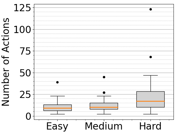
Full benchmark set. Overall, we evaluate prolex on a total of 120 benchmarks, with 40 unique tasks and 3 different environments. For each of the 40 tasks, we manually write the ground truth program in our DSL and obtain a demonstration by running the ground truth program. Figure 14 presents statistics regarding the length of these demonstrations. On average, demonstrations in the easy, medium, and hard environments consist of 11, 13, and 24 actions, respectively. Some demonstrations in the hard environment exceed 100 actions due to the large number of object instances that need to be handled.
Experimental set-up. Our experiments were conducted on a server with 64 available Intel Xeon Gold 5218 CPUs @2.30GHz, 264GB of available memory, and running Ubuntu 22.04.2. We use a time limit of 120 seconds per task in all of our experiments.
6.2. Main Results for Prolex
Our main results are presented in Figure 15, with Figure 15(a) showing the percentage of completed tasks against synthesis time. We consider a task to be completed if prolex is able to synthesize a policy within the time limit, and solved if the learned program also matches the user’s intent. We determine if a task is solved by comparing it against the ground truth program (written manually) and checking if the learned program is semantically equivalent. Since the manually written policy is intended to work in all environments, tasks classified as “solved” generalize to unseen environments.
Running time. In Figure 15(a), the three lines indicate the percentage of benchmarks (y-axis) completed with a given time limit (x-axis) for each of the three environments (Easy, Medium, Hard). Across all environments, prolex is able to complete 36% of the tasks within the first 5 seconds, 28% of the tasks within 6-30 seconds, and 16% of the tasks within 31-120 seconds. Overall, prolex is able to complete 80% of the tasks within the 2 minute time limit.
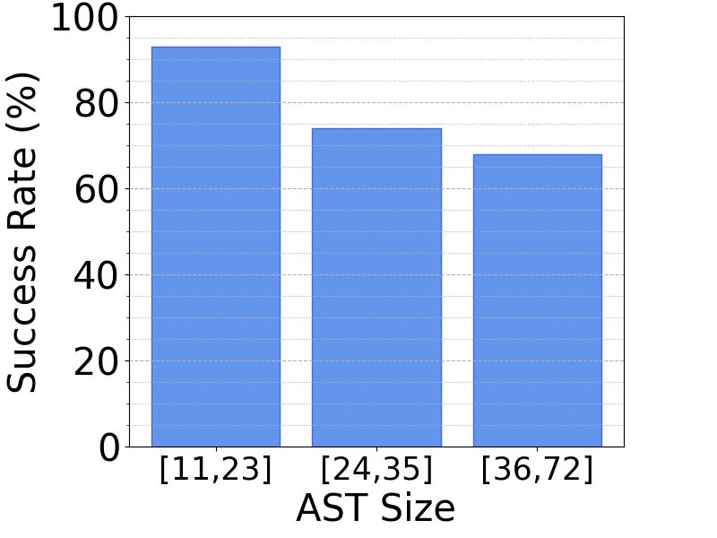
Figure 15 also provides a more detailed look at these statistics by showing the percentage of completed tasks with respect to task complexity. In particular, Figure 15(b) shows the rate of completion according to the size of the ground truth program. As expected, the learning problem becomes harder as the complexity of target policy increases. However, even for the most complex programs, prolex is still able to complete the learning task for 68% of the benchmarks.


Generalizability. As mentioned earlier, completing a task is not the same as “solving” it, since the synthesized policy may not match user intent despite being consistent with the demonstrations. We manually inspected all programs synthesized by prolex and found that it is equivalent to the ground truth program in 81% of the completed cases. Interestingly, as shown in Figure 15(c), we found that prolex’s generalization power improves as environment complexity increases. Intuitively, the more complex the environment, the more objects there are with different properties, so it becomes harder to find multiple programs that “touch” exactly the same objects as the demonstration.
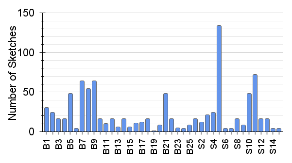
Search Statistics. As explained in Section 4, sketches in prolex are enumerated based on increasing order of complexity. In each iteration, a finite number of completions are considered for the current sketch. If none of these completions aligns with the demonstrations, the algorithm advances to the next sketch. This process continues until either a successful match is found or the time limit is reached. Figure 16 presents the average number of sketches encountered before finding the solution or timing out for each task in all three environments. For almost all tasks, prolex considers fewer than 50 sketches before termination. One task () is exceptionally challenging and requires 143 sketches before a solution is found.
Failure analysis. As discussed above, there are two reasons why prolex may fail to solve a task: (1) it fails to find a policy consistent with the demonstrations within the time limit, or (2) the synthesized policy does not adequately capture the user intent. We have manually inspected both classes of failure cases and report on our findings.
The main cause of prolex’s timeouts is due to perception operations. Many of our environments contain a large number of object types, all of which can be arguments of operations. Our approach tries to overcome this issue by using an LLM to guide search, but in some cases, the LLM proposes the wrong object type to scan for. This causes the synthesizer to go down a rabbit hole, particularly in cases when the proposed object type has many properties associated with it. We believe more advanced LLMs that can reason about finer-grained properties between the environment and the context of the task can potentially mitigate this issue.
We also inspected the cases where prolex finds a robot execution policy consistent with the demonstrations, but the synthesized policy does not generalize to different environments (i.e., it completes the task but fails to solve it). There are two main reasons for this, both due to the inadequacy of the demonstrations with respect to the desired task. Specifically, if there is only one instance of a particular object type in the environment, the synthesizer may not return a program with a loop over that object type, even though the ground truth program contains such a loop. Likewise, prolex is capable of inferring conditional blocks only if the demonstrations are branch complete. This means that, in the demonstration environment, some instances of a manipulated object type must satisfy the intended property, while others must not. If all (or none) of the object instances of that type are acted upon, the synthesizer cannot learn the conditional block for such manipulations. As noted earlier, this generalizability issue becomes less of a problem in more complex environments with many instances of an object type.
RQ1 Summary. Given a 2 minute time limit, prolex is able to find a policy consistent with the demonstations for 80% of the benchmarks. Furthermore 81% of the synthesized programs correspond to the ground truth, meaning that they can generalize to any unseen environment.
6.3. Ablation Studies
As mentioned throughout the paper, there are three key components underlying our approach, namely (1) learning control flow structures (i.e., sketches), (2) use of LLMs to guide sketch completion, and (3) new technique for proving unrealizability. To better understand the relative importance of each component, we present the results of an ablation study where we disable each component or combinations of components. Specifically, for our ablation study, we consider the following variants of prolex:
-
•
prolex-NoSketch: This is a variant of prolex that does not generate program sketches using regex learning.
-
•
prolex-NoLLM: This is a variant of prolex that does not utilize LLMs for sketch completion.
-
•
prolex-NoPrune: This is a variant of prolex that does not utilize the unrealizability checking procedure (Algorithm 2) for pruning the search space during sketch completion.
-
•
prolex-SketchOnly: This is a variant of prolex that infers control flow sketches (through regex learning) but neither utilizes LLM nor unrealizability checking during sketch completion.
-
•
prolex-NoLoopBound: This is a variant of prolex summarizes loops using the Kleene star operator during the unrealizability checking procedure. That is, it does not reason about the number of loop iterations; however, it is the same as the full prolex tool otherwise.
Figure 17(a) shows the results of our ablation study in the form of a Cumulative Distribution Function (CDF). The x-axis represents the cumulative running time, while the y-axis shows the percentage of benchmarks solved in all environments. The results indicate a significant gap between the number of the tasks solved by prolex and its variants defined above. In particular, prolex is able to solve 8% more tasks than NoLLM, 19% more tasks than NoPrune, 24% more tasks than SketchOnly, and 8% more tasks than NoLoopBound variants. However, the results for the NoSketch variant are particularly poor, with none of the tasks solved.
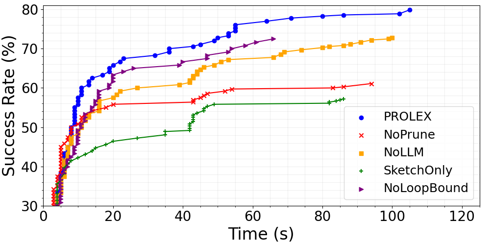
RQ2 Summary. All of the key components of our proposed synthesis algorithm contribute to the practicality of our learning approach. The most important component is regex-based sketch generation, without which none of the tasks can be solved. The unrealizability checking procedure helps solve an additional 18% of the tasks, and LLM guidance increases success rate by another 8%.
6.4. Comparison with Alternative Approaches
In this section, we report on our experience comparing prolex against alternative approaches. While there is no existing off-the-shelf LfD approach that targets our problem domain (see Section 6.1), we compare prolex against the following two baselines:
-
•
CVC5: We formulate our learning problem as an instance of syntax-guided synthesis and use a leading SyGuS solver, CVC5 (Barbosa et al., 2022), as a programmatic policy synthesizer.
-
•
GPT-Synth: We use an LLM as a neural program synthesizer in our domain. To this end, we consider a baseline called “GPT-Synth” that synthesizes programs in our DSL from demonstrations.
Case Study with CVC5.
Our programmatic LfD task can be reduced to an instance of the syntax-guided synthesis (SyGuS) problem (Alur et al., 2015a), which is the standard formulation for synthesis problems. To compare prolex against state-of-the-art SyGuS solvers, we encoded our tasks as instances of SyGuS and leveraged an off-the-shelf solver, namely, CVC5 (Barbosa et al., 2022), which is the winner of the most recent SyGuS competition.
To perform this comparison, we defined our DSL using the syntactic constraints in SyGuS, and we incorporated semantic constraints based on the initial and final environment states in the demonstrations. Note that SyGuS solvers are unable to perform synthesis from demonstrations, as demonstrations correspond to intermediate program states, which are not expressible in the SyGuS formulation. Hence, when comparing against CVC5, we only use the initial and final environments and consider a task to be completed if the solver returns a policy that produces the desired environment. Furthermore, we only compare the performance of prolex and CVC5 on the “easy” environment as encoding the environments in SyGuS requires significant manual labor.
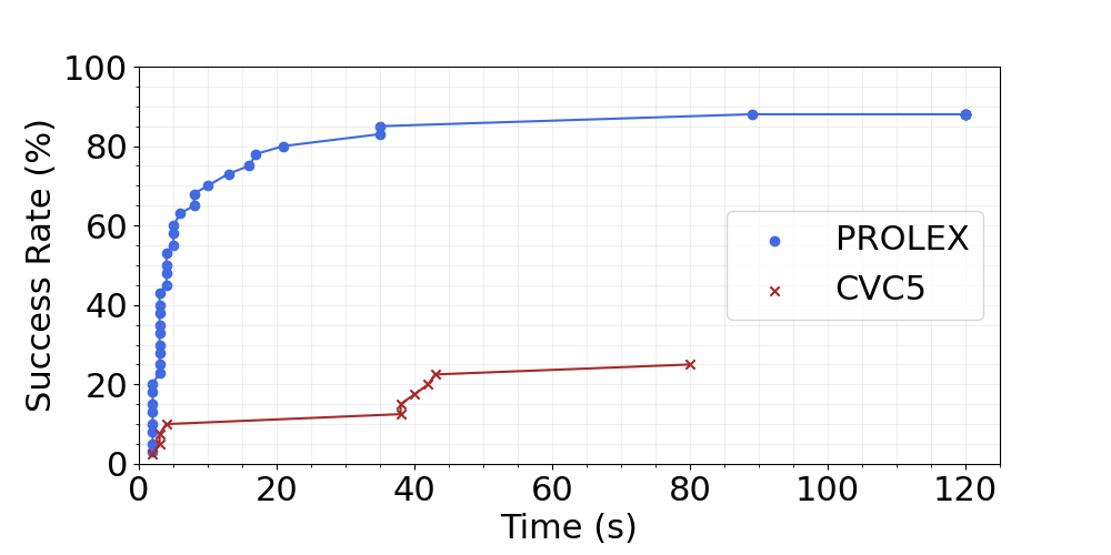
When we tried to use CVC5 to perform synthesis from scratch (i.e., without a sketch), it was not able to complete any task within a reasonable time limit. Hence, for this evaluation, we manually provided CVC5 with the ground truth sketch for the specific task. The results of this comparison are presented in Figure 17(b). As in Figure 17(a), this figure plots the cumulative distribution of the percentage of synthesized programs against solver time. Overall, CVC5 only solves of the tasks, compared to solved by prolex.
Case Study with GPT-Synth.
For this experiment, we use the GPT 3.5 LLM888We specifically use the text-davinci-003 model, which is the most capable publicly available LLM from OpenAI finetuned for completion, including natural language and code. to generate programmatic policies from demonstrations. This study aims to evaluate the effectiveness of LLMs as an end-to-end program synthesizer, henceforth referred to as GPT-Synth.
The prompts used in this study were developed using the ”template” pattern as described by White et al. (2023). This pattern has been shown to be highly effective in situations where the generated output must conform to a specific format that may not be part of the LLM’s training data. In particular, for each benchmark task, we created a prompt that includes a description of our DSL, and a set of example demonstrations and the environment states, along with the correct programs for the desired task. For a novel task, we provide the language model with the prompt, the demonstrations and environment states for the novel task, and ask it to generate a corresponding program.
To use GPT 3.5 as an end-to-end synthesizer, we adopt the following methodology, as done in prior work (Chen et al., 2021b). If the first program returned by the LLM is consistent with the demonstration, GPT-Synth returns that program as the solution. Otherwise, it asks the model to produce another program, for up to 10 iterations. Unfortunately, we found that GPT-Synth is unable to solve any of the benchmarks when we provide both the demonstrations and the environment. This behavior seems to be caused by the large number of entities and relations in the environment – prior work has reported similar results in other domains (e.g., planning (Mahowald et al., 2023)) where LLMs were used to perform tasks in non-trivial environments.
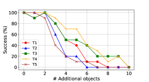
To gain more intuition about how the language model scales with the environment size, we report on our experience with using GPT-Synth on five representative tasks involving toy environments. We construct these toy environments by incorporating only the objects (and their properties) required for that task plus some additional objects and properties. Figure 18(a) shows how the success rate of GPT-Synth scales with respect to environment size. Here, the x-axis shows the number of additional objects (and their properties) in the environment and the y-axis shows the success rate. As we can see from Figure 18(a) , GPT-Synth works well if it is given only the relevant objects (which is not a realistic usage scenario), but, as environment size increases, its success rate drops dramatically. In fact, when the environment contains only 10 additional objects — a tiny fraction of our “Easy” environment — the success rate of GPT-Synth already drops to zero.
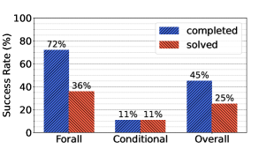
The reader may wonder if the environment is actually necessary for GPT-Synth to learn the correct program. To answer this question, we perform an additional experiment where we provide GPT-Synth with only the demonstration, but not the environment. The results of this evaluation are presented in Figure 18(b), where we classify tasks into two categories as “Forall” and “Conditional”. The former class of tasks does not involve branching, whereas the latter does. Here, “Completed” shows the percentage of tasks for which GPT-Synth finds a program consistent with the demonstration, and “Solved” shows the percentage of tasks for which GPT-Synth returns a program that also matches the ground truth. As we can see, GPT-Synth returns a program consistent with the demonstration for 45% of all tasks, but it is only able to identify the ground truth program in 25% of the cases. Furthermore, as one might expect, GPT-Synth is much more effective at the much simpler “Forall” category of tasks that involve acting on all instances of a particular type. In contrast, the “Conditional” category is much more challenging without having access to the environment, and the success rate of GPT-Synth is only 11% for this category. Intuitively, without knowing which objects have what properties, GPT-Synth has little chance of knowing that there should be a conditional and what its corresponding predicate should be. We came across a few cases where GPT-Synth is able to “hallucinate” the right predicates after several rounds of interaction; but, in general, guessing the user’s intent without knowing the environment, is at best a matter of sheer luck.
RQ3 Summary. prolex performs significantly better than the CVC5 and GPT-Synth baselines. Even when given the ground truth sketches, CVC5 is only able to return a program consistent with the final environment in 25% of the cases. On the other hand, the GPT-based synthesizer cannot solve any tasks when provided with both the demonstration and the full environment, but it is able to solve 25% of the tasks when it is given only the demonstration.
7. Related Work
Robot Learning from Demonstrations. Our approach builds upon a substantial body of literature on the use of Learning from Demonstration (LfD) techniques to learn robot execution policies (Argall et al., 2009; Sosa-Ceron et al., 2022; Argall et al., 2008). This literature can be broadly categorized into two approaches: (1) learning neural models to represent robot behaviors (Ly and Akhloufi, 2021; Sünderhauf et al., 2018; Ziebart et al., 2008; Kober et al., 2013; Ho and Ermon, 2016; Xiao et al., 2021; Taylor and Stone, 2009; Rusu et al., 2017), and (2) synthesizing programmatic representations of execution policies (Holtz et al., 2020a, 2021; Niekum et al., 2015; French et al., 2019). The most well-established techniques for learning neural models from demonstrations include behavior cloning within the framework of imitation learning (Ly and Akhloufi, 2021; Ho and Ermon, 2016) and (deep) reinforcement learning (RL) methods (Sünderhauf et al., 2018; Ziebart et al., 2008; Kober et al., 2013). Empirical studies have demonstrated the efficacy of these neural policies in perception tasks and their ability to perform well in unknown or ill-defined environments. However, such neural models lack robust interpretability and generalization capabilities — as a testament to this, there exist no neural LfD algorithms to date capable of leveraging the user demonstrations in the Behavior benchmarks (Srivastava et al., 2022). The field of transfer learning (Pan and Yang, 2010; Taylor and Stone, 2009; Rusu et al., 2017) aims to resolve generalization problems to some degree and also enhance data efficiency. A related setting to our work is applying reinforcement learning (RL) by specifying the task via formal specification of the goal conditions; in fact, the Behavior benchmark set (Srivastava et al., 2022) reports the results of such an approach. However, even in the simplest 12 activities, the RL algorithms are unable to complete the tasks even when initiated close to the goal states. Further, even when the actions are abstracted into symbols in Behavior-1K (Li et al., 2023), RL approaches demonstrate very poor performance. These results mainly highlight the complexity of the tasks that we tackle in this paper.
Recently, there has also been growing interest in developing techniques to enhance the transparency and reliability of RL systems through formal explanations (Topin and Veloso, 2019; Glanois et al., 2021; Krajna et al., 2022; Li et al., 2019). These techniques aim to explain different aspects of the learned models, such as inputs and transitions, by finding interpretable representations of neural policies, such as Abstracted Policy Graphs (Topin and Veloso, 2019) or structures in a high-level DSL (Verma et al., 2018). More recently, there has also been interest in utilizing program synthesis methods (Xin et al., 2023; Holtz et al., 2020b) to learn robot execution policies from demonstrations as an alternative to neural model learning (Holtz et al., 2020a, 2021). These approaches provide improved interpretability, generalizability (Holtz et al., 2018), and data efficiency. prolex falls into the same class of techniques as these approaches but broadens their applicability in several ways: First, it can learn policies to handle long-horizon tasks; second, it can synthesize programs with complex control flow, such as loops with nested conditionals and loops; and, third, it can handle environments with a large number of objects and properties.
Lastly, recent work proposes a methodology for automated learning of robotic programs for long-horizon human-robot interaction policies from multi-modal inputs, including demonstrations and natural language (Porfirio et al., 2019, 2023). The contributions of this work are largely complementary to ours: their main focus is an interface for allowing end-users to draw the navigation path of a robot on a 2D map of the environment and inferring symbolic traces from this raw path representation. Similar to our regex-learning-based sketch inference algorithm, the synthesizer in this work utilizes an automata learning approach to generalize user-provided traces into Mealy automata, based on the approach in (Neider, 2014). However, the control structures in their learned programs only admit restricted loops with no nesting. Additionally, this synthesizer does not produce loops over objects and locations in the environment and does not address challenges related to perception, i.e. inference of objects not present in the demonstrations.
Program Synthesis from Demonstrations. This paper is related to a long line of research on program synthesis, which aims to find a program that meets a specified requirement (Gulwani et al., 2017; Alur et al., 2015b; Solar-Lezama, 2008; Kalyan et al., 2018; Alur et al., 2015a; Bornholt et al., 2016; Gulwani, 2011; Jha et al., 2010a; Feng et al., 2018a; Chen et al., 2021a; Wang et al., 2018b, 2020). Different synthesizers adopt different types of specifications, such as input-output examples (Feser et al., 2015), demonstrations (Chasins et al., 2018), logical constraints (Miltner et al., 2022), refinement types (Polikarpova et al., 2016), or a reference implementation (Wang et al., 2019a).
Among these, our method is mostly related to the synthesizers that enable programming by demonstration (PbD) (Lau et al., 2003; Chasins et al., 2018). Existing PbD techniques generalize programs either from sequences of user actions (Dong et al., 2022; Chasins et al., 2018) or sequences of program states (Lau et al., 2003). Our approach is similar to the former, specifically similar to WebRobot (Dong et al., 2022), which can synthesize challenging programs with multiple nested loops from sequences of user actions. However, WebRobot cannot synthesize programs with conditional blocks, which are essential for successfully performing our tasks. Moreover, WebRobot is targeted at web process automation tasks and does not address robotics-related challenges, such as perception and environment complexity, that play a big role in this work.
Synthesis of Control Structures. A main focus of this paper is on the problem of inferring control structures from demonstration traces (Bar-David and Taubenfeld, 2003; Barthe et al., 2013; Biermann et al., 1975). This is a recognized and challenging problem that is studied in various synthesis methodologies, including approaches for code synthesis from black-box reference implementations (Heule et al., 2015; Jha et al., 2010b; Ji et al., 2023) and human-in-the-loop approaches for program learning (Pu et al., 2022; Newcomb and Bodík, 2019; Ferdowsifard et al., 2021). For instance, LooPy (Ferdowsifard et al., 2021) is a recent human-in-the-loop method that relies on the programmer to act as an oracle and identify properties of consecutive iterations within the body of the target loop. Unlike these approaches, prolex only requires a small number of demonstrations with no additional hints from the end-user.
There are relatively few synthesis algorithms that can infer nested loops with branching, and they typically rely on domain-specific simplifying assumptions to address these challenges. For instance, Rousillon (Chasins et al., 2018) is a recent synthesizer that deals with loops and is specifically designed for extracting tabular data from web pages. While Rousillon supports nested loops, it can only generate side-effect-free programs intended for information retrieval purposes. FrAngel (Shi et al., 2019) is a component-based synthesizer that also handles nested control structures but necessitates users to provide numerous examples, including base and corner cases. Lastly, there is a line of work focusing on loop unrolling and rerolling for low-level hardware and software optimization (Sisco et al., 2023; Ge et al., 2022; Rocha et al., 2022), using techniques such as term-rewriting (Nandi et al., 2020). We believe that our proposed sketch generation and unrealizability proving technique could be generally useful in any setting that (a) requires synthesizing complex control flow structures and (b) where the algorithm has access to execution traces.
Reactive Program Synthesis. This paper is also related to a long line of work on reactive synthesis, where the typical goal is to synthesize finite state machines (FSM) from temporal specifications (He et al., 2017; Baumeister et al., 2020; Krogmeier et al., 2020; Choi, 2021; Finkbeiner et al., 2019). Traditionally, reactive synthesis has been viewed as a game between two players – the controlled system and its environment – and solving the reactive synthesis problem boils down to finding a winning strategy for the controlled system. The reactive synthesis problem is computationally intractable for general classes of specifications, such as monadic second order logic or full linear temporal logic (Pnueli and Rosner, 1989), but work by Bloem et al. (2012) has shown that this problem can be made tractable by restricting the logic to a subclass known as GR(1) specifications. Another successful approach to enhance reactive synthesizers is bounded synthesis, where the number of states of the synthesized implementation is bounded by a constant (Finkbeiner and Klein, 2018; Finkbeiner and Schewe, 2013). Generally speaking, existing reactive synthesis method differ from our work in three major ways: First, they take as input temporal logic specifications rather than demonstrations, and, second, they are based on deductive rather than inductive synthesis. Third, the focus of reactive synthesis is on synthesizing reactive systems represented as finite state machines that take some input from the environment and respond with an output (e.g., action) for a single time step. Thus, while reactive synthesis is well-suited to low-level motor controllers (e.g., robot social navigation), they are a poor fit for long-horizon tasks, where programs need to reason about actions that may take many time-steps to complete and where the program must relate properties of the initial state to the chosen sequence of long action sequences (e.g., when a shelf has limited access, deciding to put away the groceries that go at the back of the shelf first, before those in the front).
Recent work has expanded the scope of reactive synthesis in several ways. For example, recent work by Choi (2021) proposes to combine reactive synthesis with SyGuS (syntax-guided synthesis) to synthesize a broader class of programs that both interact with the environment (i.e., are reactive) and that can also perform data processing. This technique, however, takes as input temporal stream logic (TSL) specifications modulo some background first-order theory. Furthermore, the algorithmic focus of that work is very different in that they show how to combine classical reactive synthesis with SyGuS, whereas our focus is on inductive synthesis for learning generalizable long horizon policies from a small number of demonstrations.
Another recent related work is (Das et al., 2023), which introduces a functional reactive synthesis algorithm for learning programs that match a sequence of observed grid frames and corresponding user actions. This work is similar to ours in that it also learns programs from observed traces rather than temporal specifications. They perform synthesis by combining standard functional synthesis techniques with an automata synthesis approach to discover time-varying latent state in the program. However, the focus of that work is to discover causal mechanisms in Atari-style, time-varying grid worlds. As such, their Autumn DSL is used for specifying how the next state should be computed upon the occurrence of relevant events, whereas our DSL is used to express a sequence of robot actions over a time horizon. As a result, the underlying synthesis techniques are also different: For example, they use automata learning to discover latent state, whereas we employ automata learning for the entirely different purpose of learning complex control structures.
Finally, reactive functional programs have also been integrated with probabilistic programming features to design simulators for human-robot interaction, enabling the sampling of test scenarios (Chung and Cakmak, 2022). These simulators generate complex event streams of human actions based on distributions learned from demonstrations. The synthesis strategy employed in this work involves providing a sketch of the target program as input and using probabilistic inference techniques, such as MCMC, to complete the unknown parameters.
Enhancing Synthesis using ML Models. Machine learning has proven to be highly effective for improving time and accuracy of synthesis (Pailoor et al., 2021; Cambronero et al., 2023; Verbruggen et al., 2021; Ye et al., 2020; Kalyan et al., 2018; Rahmani et al., 2021). For example, neural generators trained on partial programs (i.e., sketches) have been shown to accurately predict the full body of a method from just a few API calls or data types (Murali et al., 2017; Nye et al., 2019; Chen et al., 2020). In addition, LLMs have been utilized to guide program search (Jain et al., 2022). For example, the GPT-3 language model has been applied to mine program components and their distributions for multi-modal program synthesis tasks (Rahmani et al., 2021). Our work is similar in approach and leverages an LLM to improve program synthesis. However, to the best of knowledge, prolex is the first approach to leverage the LLM’s prior knowledge of the semantic relations between real-world entities and actions to guide the search towards reasonable completions.
A related field of research, neurosymbolic programming, seeks to combine advances in end-to-end machine learning techniques with program synthesis by leveraging compositional programming abstractions as a means of reusing learned modules across various tasks (Inala et al., 2020; Zhan et al., 2021; Chaudhuri et al., 2021; Chen et al., 2021a; Sun et al., 2022; Verma et al., 2019; Mao et al., 2019; Huang et al., 2020; Witt et al., 2023; Bowers et al., 2023). Because our current approach is based on a symbolic environment representation, it does not require a neurosymbolic DSL.
Program Sketching. Program sketches have been introduced as a syntactic framework to guide the generation of candidate programs during a search process. This approach was initially presented in (Solar-Lezama, 2008) and has since been widely used (Solar-Lezama, 2008; Solar-Lezama et al., 2006; Solar-Lezama, 2009; Bornholt et al., 2016; Dong et al., 2022; Wang et al., 2019b; Yaghmazadeh et al., 2017). While some approaches utilize program sketches that are crafted by the user, others automatically generate a sketch based on natural language (Chen et al., 2020; Yaghmazadeh et al., 2017) or reference implementation (Wang et al., 2019b). Our method also decomposes the synthesis task into two separate sketch generation and sketch completion step but utilizes regex learning to find a sketch that is likely to be a consistent generalization of the user demonstrations.
Unrealizability of Program Synthesis. Many prior techniques enhance program synthesis by establishing that a synthesis sub-problem is unrealizable (Wang et al., 2018a; Feng et al., 2018b; Lee et al., 2016; Vechev et al., 2010; Tiwari et al., 2015; Hu et al., 2019; Mechtaev et al., 2018). Existing methods typically rely on domain-specific static analysis and logical reasoning to establish unrealizability for the task of Programming by Example (PbE). For instance, various approaches have reduced this problem to a SMT instance and leveraged external solvers to find a proof of unrealizability (Hu et al., 2019; Kim et al., 2021; Feng et al., 2018b, 2017; Polikarpova et al., 2016; Farzan et al., 2022). While the general problem of unrealizability is undecidable (Madhusudan et al., 2018), some recent approaches have used abstract interpretation techniques to establish unrealizability more effectively (Wang et al., 2018a; Lee et al., 2016; Chen et al., 2020). Recently, Kim et al. (2023) proposed a Hoare-style reasoning system to formally define, establish, and explain the unrealizability of a problem, aiming to unify existing methods in this domain. Our synthesis technique also utilizes program abstractions to establish the unrealizability of a search path and prune partial programs. However, to the best of our knowledge, our approach is the first to check compatibility between user demonstrations and partial programs in order to establish unrealizability in the PbD setting. A different notion of trace compatibility has been proposed for synthesis-based transpilation (Mariano et al., 2022); however, that work differs from ours in several ways. First, they define compatibility between traces of two different programs, while ours is defined between a program and user demonstration. Second, their technique for checking compatibility between traces is very different from ours and relies on a collecting semantics (Cousot and Cousot, 1977) of the programming language.
8. Conclusions and Future Work
We proposed a new programmatic LfD approach, based on program synthesis, for learning robot execution policies for long-horizon tasks in complex environments. Our approach first generates a program sketch capturing control flow structure by generating a string abstraction of the given demonstrations and inferring a regular expression that matches those strings. In the second sketch completion phase, our algorithm performs LLM-guided top down search and utilizes a novel procedure for proving unrealizability of partial programs. The latter algorithm for proving unrealizability can be easily adapted to other PBD settings: the key idea is to generate, via static analysis, a regular expression that captures all traces of a partial program and then check whether the string representation of the demonstrations belongs to this language.
We have evaluated our implementation, prolex, on 120 benchmarks and show that prolex is able to synthesize complex policies with several (nested) loops and conditionals and that it scales to large environments containing thousands of objects and dozens of distinct objects types. Overall, given a 120 second time limit, prolex is able to find a program consistent with the demonstrations for 80% of the benchmarks. Furthermore, for 81% of the completed tasks, prolex can learn the ground truth program from a single demonstration. To put these numbers in context, we also compare prolex against two baselines, including a state-of-the-art SyGuS solver and a neural LLM-based synthesizer, and show that prolex significantly outperforms both of them.
In future work, we are interested in deploying this technique on real robots in physical environments. To this end, we plan to integrate a semantic-aware perception frontend like Kimera (Rosinol et al., 2021) to extract the symbolic state of the world as a semantic scene graph, as such a representation would be directly compatible with the prolex DSL. We are interested in building a web-based graphical interface to our robots to gather user demonstrations for deployments, building on existing robot deployment management systems like RoboFleet (Sikand et al., 2021).
Acknowledgements
We would like to thank our anonymous reviewers for their helpful and insightful feedback. This work was supported in part by NSF Awards #1762299, #1918889, #1901376, #2046955, and #2319471, as well as Google, Facebook, Amazon, Intel, and RelationalAI fellowships.
References
- (1)
- Aeronautiques et al. (1998) Constructions Aeronautiques, Adele Howe, Craig Knoblock, ISI Drew McDermott, Ashwin Ram, Manuela Veloso, Daniel Weld, David Wilkins SRI, Anthony Barrett, Dave Christianson, et al. 1998. Pddl— the planning domain definition language. Technical Report, Tech. Rep. (1998).
- Alur et al. (2015a) Rajeev Alur, Rastislav Bodík, Eric Dallal, Dana Fisman, Pranav Garg, Garvit Juniwal, Hadas Kress-Gazit, P. Madhusudan, Milo M. K. Martin, Mukund Raghothaman, Shambwaditya Saha, Sanjit A. Seshia, Rishabh Singh, Armando Solar-Lezama, Emina Torlak, and Abhishek Udupa. 2015a. Syntax-Guided Synthesis. In Dependable Software Systems Engineering. 1–25.
- Alur et al. (2015b) Rajeev Alur, Pavol Černý, and Arjun Radhakrishna. 2015b. Synthesis Through Unification. In Computer Aided Verification, Daniel Kroening and Corina S. Păsăreanu (Eds.). Springer International Publishing, Cham, 163–179.
- Argall et al. (2008) Brenna D. Argall, Brett Browning, and Manuela Veloso. 2008. Learning robot motion control with demonstration and advice-operators. In 2008 IEEE/RSJ International Conference on Intelligent Robots and Systems. 399–404. https://doi.org/10.1109/IROS.2008.4651020
- Argall et al. (2009) Brenna D. Argall, Sonia Chernova, Manuela Veloso, and Brett Browning. 2009. A survey of robot learning from demonstration. Robotics and Autonomous Systems 57, 5 (2009), 469–483. https://doi.org/10.1016/j.robot.2008.10.024
- Ashutosh et al. (2023) Kumar Ashutosh, Rohit Girdhar, Lorenzo Torresani, and Kristen Grauman. 2023. HierVL: Learning Hierarchical Video-Language Embeddings. In Proceedings of the IEEE/CVF Conference on Computer Vision and Pattern Recognition. 23066–23078.
- Bar-David and Taubenfeld (2003) Yoah Bar-David and Gadi Taubenfeld. 2003. Automatic Discovery of Mutual Exclusion Algorithms. In Proceedings of the Twenty-Second Annual Symposium on Principles of Distributed Computing (PODC ’03). Association for Computing Machinery, New York, NY, USA, 305. https://doi.org/10.1145/872035.872080
- Barbosa et al. (2022) Haniel Barbosa, Clark W. Barrett, Martin Brain, Gereon Kremer, Hanna Lachnitt, Makai Mann, Abdalrhman Mohamed, Mudathir Mohamed, Aina Niemetz, Andres Nötzli, Alex Ozdemir, Mathias Preiner, Andrew Reynolds, Ying Sheng, Cesare Tinelli, and Yoni Zohar. 2022. cvc5: A Versatile and Industrial-Strength SMT Solver. In Tools and Algorithms for the Construction and Analysis of Systems - 28th International Conference, TACAS 2022, Held as Part of the European Joint Conferences on Theory and Practice of Software, ETAPS 2022, Munich, Germany, April 2-7, 2022, Proceedings, Part I (Lecture Notes in Computer Science), Dana Fisman and Grigore Rosu (Eds.), Vol. 13243. Springer, 415–442. https://doi.org/10.1007/978-3-030-99524-9_24
- Barthe et al. (2013) Gilles Barthe, Juan Manuel Crespo, Sumit Gulwani, Cesar Kunz, and Mark Marron. 2013. From Relational Verification to SIMD Loop Synthesis. In Proceedings of the 18th ACM SIGPLAN Symposium on Principles and Practice of Parallel Programming (PPoPP ’13). Association for Computing Machinery, New York, NY, USA, 123–134. https://doi.org/10.1145/2442516.2442529
- Baumeister et al. (2020) Tom Baumeister, Bernd Finkbeiner, and Hazem Torfah. 2020. Explainable Reactive Synthesis. In Automated Technology for Verification and Analysis, Dang Van Hung and Oleg Sokolsky (Eds.). Springer International Publishing, Cham, 413–428.
- Biermann et al. (1975) A.W. Biermann, R.I. Baum, and F.E. Petry. 1975. Speeding up the Synthesis of Programs from Traces. IEEE Trans. Comput. C-24, 2 (1975), 122–136. https://doi.org/10.1109/T-C.1975.224180
- Bloem et al. (2012) Roderick Bloem, Barbara Jobstmann, Nir Piterman, Amir Pnueli, and Yaniv Saar. 2012. Synthesis of Reactive(1) designs. J. Comput. System Sci. 78, 3 (2012), 911–938. https://doi.org/10.1016/j.jcss.2011.08.007 In Commemoration of Amir Pnueli.
- Bornholt et al. (2016) James Bornholt, Emina Torlak, Dan Grossman, and Luis Ceze. 2016. Optimizing synthesis with metasketches. In ACM SIGPLAN Notices, Vol. 51. ACM, 775–788.
- Bowers et al. (2023) Matthew Bowers, Theo X. Olausson, Lionel Wong, Gabriel Grand, Joshua B. Tenenbaum, Kevin Ellis, and Armando Solar-Lezama. 2023. Top-Down Synthesis for Library Learning. Proc. ACM Program. Lang. 7, POPL, Article 41 (jan 2023), 32 pages. https://doi.org/10.1145/3571234
- Cambronero et al. (2023) José Cambronero, Sumit Gulwani, Vu Le, Daniel Perelman, Arjun Radhakrishna, Clint Simon, and Ashish Tiwari. 2023. FlashFill++: Scaling Programming by Example by Cutting to the Chase. Proc. ACM Program. Lang. 7, POPL, Article 33 (jan 2023), 30 pages. https://doi.org/10.1145/3571226
- Chasins et al. (2018) Sarah E. Chasins, Maria Mueller, and Rastislav Bodik. 2018. Rousillon: Scraping Distributed Hierarchical Web Data. In Proceedings of the 31st Annual ACM Symposium on User Interface Software and Technology (UIST ’18). Association for Computing Machinery, New York, NY, USA, 963–975. https://doi.org/10.1145/3242587.3242661
- Chaudhuri et al. (2021) Swarat Chaudhuri, Kevin Ellis, Oleksandr Polozov, Rishabh Singh, Armando Solar-Lezama, and Yisong Yue. 2021. Neurosymbolic Programming. Found. Trends Program. Lang. 7 (2021), 158–243.
- Chen et al. (2021b) Mark Chen, Jerry Tworek, Heewoo Jun, Qiming Yuan, Henrique Ponde de Oliveira Pinto, Jared Kaplan, Harri Edwards, Yuri Burda, Nicholas Joseph, Greg Brockman, Alex Ray, Raul Puri, Gretchen Krueger, Michael Petrov, Heidy Khlaaf, Girish Sastry, Pamela Mishkin, Brooke Chan, Scott Gray, Nick Ryder, Mikhail Pavlov, Alethea Power, Lukasz Kaiser, Mohammad Bavarian, Clemens Winter, Philippe Tillet, Felipe Petroski Such, Dave Cummings, Matthias Plappert, Fotios Chantzis, Elizabeth Barnes, Ariel Herbert-Voss, William Hebgen Guss, Alex Nichol, Alex Paino, Nikolas Tezak, Jie Tang, Igor Babuschkin, Suchir Balaji, Shantanu Jain, William Saunders, Christopher Hesse, Andrew N. Carr, Jan Leike, Josh Achiam, Vedant Misra, Evan Morikawa, Alec Radford, Matthew Knight, Miles Brundage, Mira Murati, Katie Mayer, Peter Welinder, Bob McGrew, Dario Amodei, Sam McCandlish, Ilya Sutskever, and Wojciech Zaremba. 2021b. Evaluating Large Language Models Trained on Code. arXiv:cs.LG/2107.03374
- Chen et al. (2021a) Qiaochu Chen, Aaron Lamoreaux, Xinyu Wang, Greg Durrett, Osbert Bastani, and Isil Dillig. 2021a. Web Question Answering with Neurosymbolic Program Synthesis. In Proceedings of the 42nd ACM SIGPLAN International Conference on Programming Language Design and Implementation (PLDI 2021). Association for Computing Machinery, New York, NY, USA, 328–343. https://doi.org/10.1145/3453483.3454047
- Chen et al. (2020) Qiaochu Chen, Xinyu Wang, Xi Ye, Greg Durrett, and Isil Dillig. 2020. Multi-modal synthesis of regular expressions. In Proceedings of the 41st ACM SIGPLAN conference on programming language design and implementation. 487–502.
- Choi (2021) Wonhyuk Choi. 2021. Can Reactive Synthesis and Syntax-Guided Synthesis Be Friends?. In Companion Proceedings of the 2021 ACM SIGPLAN International Conference on Systems, Programming, Languages, and Applications: Software for Humanity (SPLASH Companion 2021). Association for Computing Machinery, New York, NY, USA, 3–5. https://doi.org/10.1145/3484271.3484972
- Chung and Cakmak (2022) Michael Jae-Yoon Chung and Maya Cakmak. 2022. Authoring Human Simulators via Probabilistic Functional Reactive Program Synthesis. In 2022 17th ACM/IEEE International Conference on Human-Robot Interaction (HRI). 727–730. https://doi.org/10.1109/HRI53351.2022.9889630
- Cousot and Cousot (1977) Patrick Cousot and Radhia Cousot. 1977. Abstract Interpretation: A Unified Lattice Model for Static Analysis of Programs by Construction or Approximation of Fixpoints. 238–252.
- Das et al. (2023) Ria Das, Joshua B. Tenenbaum, Armando Solar-Lezama, and Zenna Tavares. 2023. Combining Functional and Automata Synthesis to Discover Causal Reactive Programs. Proc. ACM Program. Lang. 7, POPL, Article 56 (jan 2023), 31 pages. https://doi.org/10.1145/3571249
- Devlin et al. (2019) Jacob Devlin, Ming-Wei Chang, Kenton Lee, and Kristina Toutanova. 2019. BERT: Pre-training of Deep Bidirectional Transformers for Language Understanding. In Proceedings of the 2019 Conference of the North American Chapter of the Association for Computational Linguistics: Human Language Technologies, NAACL-HLT 2019, Minneapolis, MN, USA, June 2-7, 2019, Volume 1 (Long and Short Papers), Jill Burstein, Christy Doran, and Thamar Solorio (Eds.). Association for Computational Linguistics, 4171–4186. https://doi.org/10.18653/v1/n19-1423
- Dong et al. (2022) Rui Dong, Zhicheng Huang, Ian Iong Lam, Yan Chen, and Xinyu Wang. 2022. WebRobot: Web Robotic Process Automation Using Interactive Programming-by-Demonstration. In Proceedings of the 43rd ACM SIGPLAN International Conference on Programming Language Design and Implementation (PLDI 2022). Association for Computing Machinery, New York, NY, USA, 152–167. https://doi.org/10.1145/3519939.3523711
- Farzan et al. (2022) Azadeh Farzan, Danya Lette, and Victor Nicolet. 2022. Recursion Synthesis with Unrealizability Witnesses. In Proceedings of the 43rd ACM SIGPLAN International Conference on Programming Language Design and Implementation (PLDI 2022). Association for Computing Machinery, New York, NY, USA, 244–259. https://doi.org/10.1145/3519939.3523726
- Feng et al. (2018a) Yu Feng, Ruben Martins, Osbert Bastani, and Isil Dillig. 2018a. Program Synthesis Using Conflict-Driven Learning. In Proceedings of the 39th ACM SIGPLAN Conference on Programming Language Design and Implementation (PLDI 2018). Association for Computing Machinery, New York, NY, USA, 420–435. https://doi.org/10.1145/3192366.3192382
- Feng et al. (2018b) Yu Feng, Ruben Martins, Osbert Bastani, and Isil Dillig. 2018b. Program synthesis using conflict-driven learning. In ACM SIGPLAN Notices, Vol. 53. ACM, 420–435.
- Feng et al. (2017) Yu Feng, Ruben Martins, Jacob Van Geffen, Isil Dillig, and Swarat Chaudhuri. 2017. Component-based synthesis of table consolidation and transformation tasks from examples. In Proc. of PLDI. 422–436.
- Ferdowsifard et al. (2021) Kasra Ferdowsifard, Shraddha Barke, Hila Peleg, Sorin Lerner, and Nadia Polikarpova. 2021. LooPy: Interactive Program Synthesis with Control Structures. Proc. ACM Program. Lang. 5, OOPSLA, Article 153 (oct 2021), 29 pages. https://doi.org/10.1145/3485530
- Feser et al. (2015) John K Feser, Swarat Chaudhuri, and Isil Dillig. 2015. Synthesizing data structure transformations from input-output examples. ACM SIGPLAN Notices 50, 6 (2015), 229–239.
- Finkbeiner and Klein (2018) Bernd Finkbeiner and Felix Klein. 2018. Reactive Synthesis: Towards Output-Sensitive Algorithms. arXiv:cs.LO/1803.10104
- Finkbeiner et al. (2019) Bernd Finkbeiner, Felix Klein, Ruzica Piskac, and Mark Santolucito. 2019. Synthesizing Functional Reactive Programs. In Proceedings of the 12th ACM SIGPLAN International Symposium on Haskell (Haskell 2019). Association for Computing Machinery, New York, NY, USA, 162–175. https://doi.org/10.1145/3331545.3342601
- Finkbeiner and Schewe (2013) Bernd Finkbeiner and Sven Schewe. 2013. Bounded synthesis. International Journal on Software Tools for Technology Transfer 15, 5-6 (2013), 519–539.
- Fox and Long (2003) Maria Fox and Derek Long. 2003. PDDL2. 1: An extension to PDDL for expressing temporal planning domains. Journal of artificial intelligence research 20 (2003), 61–124.
- French et al. (2019) Kevin French, Shiyu Wu, Tianyang Pan, Zheming Zhou, and Odest Chadwicke Jenkins. 2019. Learning Behavior Trees From Demonstration. In 2019 International Conference on Robotics and Automation (ICRA). 7791–7797. https://doi.org/10.1109/ICRA.2019.8794104
- Ge et al. (2022) Tianao Ge, Zewei Mo, Kan Wu, Xianwei Zhang, and Yutong Lu. 2022. RollBin: Reducing Code-Size via Loop Rerolling at Binary Level. In Proceedings of the 23rd ACM SIGPLAN/SIGBED International Conference on Languages, Compilers, and Tools for Embedded Systems (LCTES 2022). Association for Computing Machinery, New York, NY, USA, 99–110. https://doi.org/10.1145/3519941.3535072
- Glanois et al. (2021) Claire Glanois, Paul Weng, Matthieu Zimmer, Dong Li, Tianpei Yang, Jianye Hao, and Wulong Liu. 2021. A Survey on Interpretable Reinforcement Learning. https://doi.org/10.48550/ARXIV.2112.13112
- Gulwani (2011) Sumit Gulwani. 2011. Automating string processing in spreadsheets using input-output examples. In Proc. of POPL. 317–330.
- Gulwani et al. (2017) Sumit Gulwani, Oleksandr Polozov, and Rishabh Singh. 2017. Program Synthesis. Foundations and Trends in Programming Languages 4, 1-2, 1–119.
- He et al. (2017) Keliang He, Morteza Lahijanian, Lydia E. Kavraki, and Moshe Y. Vardi. 2017. Reactive synthesis for finite tasks under resource constraints. In 2017 IEEE/RSJ International Conference on Intelligent Robots and Systems (IROS). 5326–5332. https://doi.org/10.1109/IROS.2017.8206426
- Heule et al. (2015) Stefan Heule, Manu Sridharan, and Satish Chandra. 2015. Mimic: Computing Models for Opaque Code. In Proceedings of the 2015 10th Joint Meeting on Foundations of Software Engineering (ESEC/FSE 2015). Association for Computing Machinery, New York, NY, USA, 710–720. https://doi.org/10.1145/2786805.2786875
- Ho and Ermon (2016) Jonathan Ho and Stefano Ermon. 2016. Generative Adversarial Imitation Learning. In Advances in Neural Information Processing Systems, D. Lee, M. Sugiyama, U. Luxburg, I. Guyon, and R. Garnett (Eds.), Vol. 29. Curran Associates, Inc. https://proceedings.neurips.cc/paper/2016/file/cc7e2b878868cbae992d1fb743995d8f-Paper.pdf
- Holtz et al. (2021) Jarrett Holtz, Simon Andrews, Arjun Guha, and Joydeep Biswas. 2021. Iterative Program Synthesis for Adaptable Social Navigation. In Intelligent Robots and Systems (IROS), IEEE/RSJ International Conference on. 6256–6261. https://doi.org/10.1109/IROS51168.2021.9636540
- Holtz et al. (2018) Jarrett Holtz, Arjun Guha, and Joydeep Biswas. 2018. Interactive Robot Transition Repair With SMT. In International Joint Conference on Artificial Intelligence (IJCAI). 4905–4911. https://doi.org/10.24963/ijcai.2018/681
- Holtz et al. (2020a) Jarrett Holtz, Arjun Guha, and Joydeep Biswas. 2020a. Robot Action Selection Learning via Layered Dimension Informed Program Synthesis. In Conference on Robot Learning. 1471–1480. https://joydeepb.com/Publications/corl2020_ldips.pdf
- Holtz et al. (2020b) Jarrett Holtz, Arjun Guha, and Joydeep Biswas. 2020b. Robot Action Selection Learning via Layered Dimension Informed Program Synthesis. In Conference on Robot Learning.
- Hu et al. (2019) Qinheping Hu, Jason Breck, John Cyphert, Loris D’Antoni, and Thomas Reps. 2019. Proving Unrealizability for Syntax-Guided Synthesis. In Computer Aided Verification, Isil Dillig and Serdar Tasiran (Eds.). Springer International Publishing, Cham, 335–352.
- Huang et al. (2020) Jiani Huang, Calvin Smith, Osbert Bastani, Rishabh Singh, Aws Albarghouthi, and Mayur Naik. 2020. Generating Programmatic Referring Expressions via Program Synthesis. In Proceedings of the 37th International Conference on Machine Learning (Proceedings of Machine Learning Research), Hal Daumé III and Aarti Singh (Eds.), Vol. 119. PMLR, 4495–4506. https://proceedings.mlr.press/v119/huang20h.html
- Inala et al. (2020) Jeevana Priya Inala, Yichen Yang, James Paulos, Yewen Pu, Osbert Bastani, Vijay Kumar, Martin Rinard, and Armando Solar-Lezama. 2020. Neurosymbolic Transformers for Multi-Agent Communication. In Proceedings of the 34th International Conference on Neural Information Processing Systems (NIPS’20). Curran Associates Inc., Red Hook, NY, USA, Article 1141, 12 pages.
- iRobot (2023) iRobot. 2023. iRobot Home App. https://www.irobot.com/en_US/irobot-home-app.html Accessed on March 30, 2023.
- Jain et al. (2022) Naman Jain, Skanda Vaidyanath, Arun Iyer, Nagarajan Natarajan, Suresh Parthasarathy, Sriram Rajamani, and Rahul Sharma. 2022. Jigsaw: Large Language Models Meet Program Synthesis. In Proceedings of the 44th International Conference on Software Engineering (ICSE ’22). Association for Computing Machinery, New York, NY, USA, 1219–1231. https://doi.org/10.1145/3510003.3510203
- Jha et al. (2010a) Susmit Jha, Sumit Gulwani, Sanjit A Seshia, and Ashish Tiwari. 2010a. Oracle-guided component-based program synthesis. In 2010 ACM/IEEE 32nd International Conference on Software Engineering, Vol. 1. IEEE, 215–224.
- Jha et al. (2010b) Susmit Jha, Sumit Gulwani, Sanjit A. Seshia, and Ashish Tiwari. 2010b. Oracle-Guided Component-Based Program Synthesis. In Proceedings of the 32nd ACM/IEEE International Conference on Software Engineering - Volume 1 (ICSE ’10). Association for Computing Machinery, New York, NY, USA, 215–224. https://doi.org/10.1145/1806799.1806833
- Ji et al. (2023) Ruyi Ji, Chaozhe Kong, Yingfei Xiong, and Zhenjiang Hu. 2023. Improving Oracle-Guided Inductive Synthesis by Efficient Question Selection. Proc. ACM Program. Lang. 7, OOPSLA1, Article 103 (apr 2023), 29 pages. https://doi.org/10.1145/3586055
- Kalyan et al. (2018) Ashwin Kalyan, Abhishek Mohta, Oleksandr Polozov, Dhruv Batra, Prateek Jain, and Sumit Gulwani. 2018. Neural-Guided Deductive Search for Real-Time Program Synthesis from Examples. https://doi.org/10.48550/ARXIV.1804.01186
- Kim et al. (2023) Jinwoo Kim, Loris D’Antoni, and Thomas Reps. 2023. Unrealizability Logic. Proc. ACM Program. Lang. 7, POPL, Article 23 (jan 2023), 30 pages. https://doi.org/10.1145/3571216
- Kim et al. (2021) Jinwoo Kim, Qinheping Hu, Loris D’Antoni, and Thomas Reps. 2021. Semantics-Guided Synthesis. Proc. ACM Program. Lang. 5, POPL, Article 30 (jan 2021), 32 pages. https://doi.org/10.1145/3434311
- Kober et al. (2013) Jens Kober, J. Andrew Bagnell, and Jan Peters. 2013. Reinforcement learning in robotics: A survey. The International Journal of Robotics Research 32, 11 (2013), 1238–1274. https://doi.org/10.1177/0278364913495721 arXiv:https://doi.org/10.1177/0278364913495721
- Krajna et al. (2022) Agneza Krajna, Mario Brcic, Tomislav Lipic, and Juraj Doncevic. 2022. Explainability in reinforcement learning: perspective and position. https://doi.org/10.48550/ARXIV.2203.11547
- Krogmeier et al. (2020) Paul Krogmeier, Umang Mathur, Adithya Murali, P. Madhusudan, and Mahesh Viswanathan. 2020. Decidable Synthesis of Programs with Uninterpreted Functions. In Computer Aided Verification, Shuvendu K. Lahiri and Chao Wang (Eds.). Springer International Publishing, Cham, 634–657.
- Lau et al. (2003) Tessa A. Lau, Steven A. Wolfman, Pedro M. Domingos, and Daniel S. Weld. 2003. Programming by Demonstration Using Version Space Algebra. Machine Learning 53 (2003), 111–156.
- Lee et al. (2023) Jin Joo Lee, Amin Atrash, Dylan Glas, and Hanxiao Fu. 2023. Developing autonomous behaviors for a consumer robot to hang out near people in the home. In AAAI 2023 Spring Symposium Series. https://www.amazon.science/publications/developing-autonomous-behaviors-for-a-consumer-robot-to-hang-out-near-people-in-the-home
- Lee et al. (2016) Mina Lee, Sunbeom So, and Hakjoo Oh. 2016. Synthesizing Regular Expressions from Examples for Introductory Automata Assignments. In Proceedings of the 2016 ACM SIGPLAN International Conference on Generative Programming: Concepts and Experiences (GPCE 2016). Association for Computing Machinery, New York, NY, USA, 70–80. https://doi.org/10.1145/2993236.2993244
- Li et al. (2023) Chengshu Li, Ruohan Zhang, Josiah Wong, Cem Gokmen, Sanjana Srivastava, Roberto Martín-Martín, Chen Wang, Gabrael Levine, Michael Lingelbach, Jiankai Sun, Mona Anvari, Minjune Hwang, Manasi Sharma, Arman Aydin, Dhruva Bansal, Samuel Hunter, Kyu-Young Kim, Alan Lou, Caleb R Matthews, Ivan Villa-Renteria, Jerry Huayang Tang, Claire Tang, Fei Xia, Silvio Savarese, Hyowon Gweon, Karen Liu, Jiajun Wu, and Li Fei-Fei. 2023. BEHAVIOR-1K: A Benchmark for Embodied AI with 1,000 Everyday Activities and Realistic Simulation. In Proceedings of The 6th Conference on Robot Learning (Proceedings of Machine Learning Research), Karen Liu, Dana Kulic, and Jeff Ichnowski (Eds.), Vol. 205. PMLR, 80–93. https://proceedings.mlr.press/v205/li23a.html
- Li et al. (2019) Xiao Li, Zachary Serlin, Guang Yang, and Calin Belta. 2019. A formal methods approach to interpretable reinforcement learning for robotic planning. Science Robotics 4, 37 (2019), eaay6276. https://doi.org/10.1126/scirobotics.aay6276 arXiv:https://www.science.org/doi/pdf/10.1126/scirobotics.aay6276
- Liang et al. (2022) Jacky Liang, Wenlong Huang, Fei Xia, Peng Xu, Karol Hausman, Brian Ichter, Pete Florence, and Andy Zeng. 2022. Code as policies: Language model programs for embodied control. arXiv preprint arXiv:2209.07753 (2022).
- Lipton (2018) Zachary C. Lipton. 2018. The Mythos of Model Interpretability: In Machine Learning, the Concept of Interpretability is Both Important and Slippery. Queue 16, 3 (jun 2018), 31–57. https://doi.org/10.1145/3236386.3241340
- Liu et al. (2023) Pengfei Liu, Weizhe Yuan, Jinlan Fu, Zhengbao Jiang, Hiroaki Hayashi, and Graham Neubig. 2023. Pre-Train, Prompt, and Predict: A Systematic Survey of Prompting Methods in Natural Language Processing. ACM Comput. Surv. 55, 9, Article 195 (jan 2023), 35 pages. https://doi.org/10.1145/3560815
- Ly and Akhloufi (2021) Abdoulaye O. Ly and Moulay Akhloufi. 2021. Learning to Drive by Imitation: An Overview of Deep Behavior Cloning Methods. IEEE Transactions on Intelligent Vehicles 6, 2 (2021), 195–209. https://doi.org/10.1109/TIV.2020.3002505
- Madhusudan et al. (2018) P. Madhusudan, Umang Mathur, Shambwaditya Saha, and Mahesh Viswanathan. 2018. A Decidable Fragment of Second Order Logic With Applications to Synthesis. In 27th EACSL Annual Conference on Computer Science Logic (CSL 2018) (Leibniz International Proceedings in Informatics (LIPIcs)), Dan Ghica and Achim Jung (Eds.), Vol. 119. Schloss Dagstuhl–Leibniz-Zentrum fuer Informatik, Dagstuhl, Germany, 31:1–31:19. https://doi.org/10.4230/LIPIcs.CSL.2018.31
- Mahowald et al. (2023) Kyle Mahowald, Anna A Ivanova, Idan A Blank, Nancy Kanwisher, Joshua B Tenenbaum, and Evelina Fedorenko. 2023. Dissociating language and thought in large language models: a cognitive perspective. arXiv preprint arXiv:2301.06627 (2023).
- Mao et al. (2019) Jiayuan Mao, Chuang Gan, Pushmeet Kohli, Joshua B. Tenenbaum, and Jiajun Wu. 2019. The Neuro-Symbolic Concept Learner: Interpreting Scenes, Words, and Sentences From Natural Supervision. In International Conference on Learning Representations. https://openreview.net/forum?id=rJgMlhRctm
- Mariano et al. (2022) Benjamin Mariano, Yanju Chen, Yu Feng, Greg Durrett, and Işil Dillig. 2022. Automated Transpilation of Imperative to Functional Code Using Neural-Guided Program Synthesis. Proc. ACM Program. Lang. 6, OOPSLA1, Article 71 (apr 2022), 27 pages. https://doi.org/10.1145/3527315
- Mechtaev et al. (2018) Sergey Mechtaev, Alberto Griggio, Alessandro Cimatti, and Abhik Roychoudhury. 2018. Symbolic Execution with Existential Second-Order Constraints. In Proceedings of the 2018 26th ACM Joint Meeting on European Software Engineering Conference and Symposium on the Foundations of Software Engineering (ESEC/FSE 2018). Association for Computing Machinery, New York, NY, USA, 389–399. https://doi.org/10.1145/3236024.3236049
- Michael L. Scott (2000) Michael Lee Michael L. Scott. 2000. Programming language pragmatics. Morgan Kaufmann.
- Miltner et al. (2022) Anders Miltner, Adrian Trejo Nuñez, Ana Brendel, Swarat Chaudhuri, and Isil Dillig. 2022. Bottom-up Synthesis of Recursive Functional Programs Using Angelic Execution. Proc. ACM Program. Lang. 6, POPL, Article 21 (jan 2022), 29 pages. https://doi.org/10.1145/3498682
- Murali et al. (2017) Vijayaraghavan Murali, Letao Qi, Swarat Chaudhuri, and Chris Jermaine. 2017. Neural Sketch Learning for Conditional Program Generation. https://doi.org/10.48550/ARXIV.1703.05698
- Nandi et al. (2020) Chandrakana Nandi, Max Willsey, Adam Anderson, James R. Wilcox, Eva Darulova, Dan Grossman, and Zachary Tatlock. 2020. Synthesizing Structured CAD Models with Equality Saturation and Inverse Transformations. In Proceedings of the 41st ACM SIGPLAN Conference on Programming Language Design and Implementation (PLDI 2020). Association for Computing Machinery, New York, NY, USA, 31–44. https://doi.org/10.1145/3385412.3386012
- Nazarczuk and Mikolajczyk (2020) Michal Nazarczuk and Krystian Mikolajczyk. 2020. V2A-Vision to Action: Learning robotic arm actions based on vision and language. In Proceedings of the Asian Conference on Computer Vision.
- Neider (2014) Daniel Neider. 2014. Applications of automata learning in verification and synthesis.
- Newcomb and Bodík (2019) Julie L. Newcomb and Rastislav Bodík. 2019. Using human-in-the-loop synthesis to author functional reactive programs. ArXiv abs/1909.11206 (2019). https://d-nb.info/1059276062/34
- Niekum et al. (2015) Scott Niekum, Sarah Osentoski, George Konidaris, Sachin Chitta, Bhaskara Marthi, and Andrew G. Barto. 2015. Learning grounded finite-state representations from unstructured demonstrations. The International Journal of Robotics Research 34, 2 (2015), 131–157. https://doi.org/10.1177/0278364914554471 arXiv:https://doi.org/10.1177/0278364914554471
- Nordmann (2014) Kore Nordmann. 2014. XML-Schema-learner. https://github.com/kore/XML-Schema-learner.
- Nye et al. (2019) Maxwell Nye, Luke Hewitt, Joshua Tenenbaum, and Armando Solar-Lezama. 2019. Learning to Infer Program Sketches. https://doi.org/10.48550/ARXIV.1902.06349
- Pailoor et al. (2021) Shankara Pailoor, Yuepeng Wang, Xinyu Wang, and Isil Dillig. 2021. Synthesizing Data Structure Refinements from Integrity Constraints. In Proceedings of the 42nd ACM SIGPLAN International Conference on Programming Language Design and Implementation (PLDI 2021). Association for Computing Machinery, New York, NY, USA, 574–587. https://doi.org/10.1145/3453483.3454063
- Pan and Yang (2010) Sinno Jialin Pan and Qiang Yang. 2010. A Survey on Transfer Learning. IEEE Transactions on Knowledge and Data Engineering 22 (2010), 1345–1359.
- Pnueli and Rosner (1989) A. Pnueli and R. Rosner. 1989. On the Synthesis of a Reactive Module. In Proceedings of the 16th ACM SIGPLAN-SIGACT Symposium on Principles of Programming Languages (POPL ’89). Association for Computing Machinery, New York, NY, USA, 179–190. https://doi.org/10.1145/75277.75293
- Polikarpova et al. (2016) Nadia Polikarpova, Ivan Kuraj, and Armando Solar-Lezama. 2016. Program synthesis from polymorphic refinement types. In Proc. of PLDI. 522–538.
- Porfirio et al. (2019) David Porfirio, Evan Fisher, Allison Sauppé, Aws Albarghouthi, and Bilge Mutlu. 2019. Bodystorming Human-Robot Interactions. In Proceedings of the 32nd Annual ACM Symposium on User Interface Software and Technology (UIST ’19). Association for Computing Machinery, New York, NY, USA, 479–491. https://doi.org/10.1145/3332165.3347957
- Porfirio et al. (2023) David Porfirio, Laura Stegner, Maya Cakmak, Allison Sauppé, Aws Albarghouthi, and Bilge Mutlu. 2023. Sketching Robot Programs On the Fly. In Proceedings of the 2023 ACM/IEEE International Conference on Human-Robot Interaction (HRI ’23). Association for Computing Machinery, New York, NY, USA, 584–593. https://doi.org/10.1145/3568162.3576991
- Pu et al. (2022) Kevin Pu, Rainey Fu, Rui Dong, Xinyu Wang, Yan Chen, and Tovi Grossman. 2022. SemanticOn: Specifying Content-Based Semantic Conditions for Web Automation Programs. In Proceedings of the 35th Annual ACM Symposium on User Interface Software and Technology (UIST ’22). Association for Computing Machinery, New York, NY, USA, Article 63, 16 pages. https://doi.org/10.1145/3526113.3545691
- Rahmani et al. (2021) Kia Rahmani, Mohammad Raza, Sumit Gulwani, Vu Le, Daniel Morris, Arjun Radhakrishna, Gustavo Soares, and Ashish Tiwari. 2021. Multi-Modal Program Inference: A Marriage of Pre-Trained Language Models and Component-Based Synthesis. Proc. ACM Program. Lang. 5, OOPSLA, Article 158 (oct 2021), 29 pages. https://doi.org/10.1145/3485535
- Rocha et al. (2022) Rodrigo C. O. Rocha, Pavlos Petoumenos, Björn Franke, Pramod Bhatotia, and Michael O’Boyle. 2022. Loop Rolling for Code Size Reduction. In Proceedings of the 20th IEEE/ACM International Symposium on Code Generation and Optimization (CGO ’22). IEEE Press, 217–229. https://doi.org/10.1109/CGO53902.2022.9741256
- Rosinol et al. (2021) Antoni Rosinol, Andrew Violette, Marcus Abate, Nathan Hughes, Yun Chang, Jingnan Shi, Arjun Gupta, and Luca Carlone. 2021. Kimera: From SLAM to spatial perception with 3D dynamic scene graphs. The International Journal of Robotics Research 40, 12-14 (2021), 1510–1546.
- Rusu et al. (2017) Andrei A. Rusu, Matej Vecerík, Thomas Rothörl, Nicolas Heess, Razvan Pascanu, and Raia Hadsell. 2017. Sim-to-Real Robot Learning from Pixels with Progressive Nets. In 1st Annual Conference on Robot Learning, CoRL 2017, Mountain View, California, USA, November 13-15, 2017, Proceedings (Proceedings of Machine Learning Research), Vol. 78. PMLR, 262–270. http://proceedings.mlr.press/v78/rusu17a.html
- Shi et al. (2019) Kensen Shi, Jacob Steinhardt, and Percy Liang. 2019. FrAngel: Component-Based Synthesis with Control Structures. Proc. ACM Program. Lang. 3, POPL, Article 73 (jan 2019), 29 pages. https://doi.org/10.1145/3290386
- Sikand et al. (2021) Kavan Singh Sikand, Logan Zartman, Sadegh Rabiee, and Joydeep Biswas. 2021. Robofleet: Open source communication and management for fleets of autonomous robots. In 2021 IEEE/RSJ International Conference on Intelligent Robots and Systems (IROS). IEEE, 406–412.
- Sisco et al. (2023) Zachary D. Sisco, Jonathan Balkind, Timothy Sherwood, and Ben Hardekopf. 2023. Loop Rerolling for Hardware Decompilation. Proc. ACM Program. Lang. 7, PLDI, Article 123 (jun 2023), 23 pages. https://doi.org/10.1145/3591237
- Solar-Lezama (2008) Armando Solar-Lezama. 2008. Program synthesis by sketching. Citeseer.
- Solar-Lezama (2009) Armando Solar-Lezama. 2009. The Sketching Approach to Program Synthesis. In Proc. of APLAS. 4–13.
- Solar-Lezama et al. (2006) Armando Solar-Lezama, Liviu Tancau, Rastislav Bodík, Sanjit A. Seshia, and Vijay A. Saraswat. 2006. Combinatorial sketching for finite programs. In Proc. of ASPLOS. 404–415.
- Sosa-Ceron et al. (2022) Arturo Daniel Sosa-Ceron, Hugo Gustavo Gonzalez-Hernandez, and Jorge Antonio Reyes-Avendaño. 2022. Learning from Demonstrations in Human and Robot Collaborative Scenarios: A Survey. Robotics 11, 6 (2022). https://doi.org/10.3390/robotics11060126
- Srivastava et al. (2022) Sanjana Srivastava, Chengshu Li, Michael Lingelbach, Roberto Martín-Martín, Fei Xia, Kent Elliott Vainio, Zheng Lian, Cem Gokmen, Shyamal Buch, Karen Liu, Silvio Savarese, Hyowon Gweon, Jiajun Wu, and Li Fei-Fei. 2022. BEHAVIOR: Benchmark for Everyday Household Activities in Virtual, Interactive, and Ecological Environments. In Proceedings of the 5th Conference on Robot Learning (Proceedings of Machine Learning Research), Aleksandra Faust, David Hsu, and Gerhard Neumann (Eds.), Vol. 164. PMLR, 477–490. https://proceedings.mlr.press/v164/srivastava22a.html
- Sun et al. (2022) Jennifer J. Sun, Megan Tjandrasuwita, Atharva Sehgal, Armando Solar-Lezama, Swarat Chaudhuri, Yisong Yue, and Omar Costilla-Reyes. 2022. Neurosymbolic Programming for Science. https://doi.org/10.48550/ARXIV.2210.05050
- Sünderhauf et al. (2018) Niko Sünderhauf, Oliver Brock, Walter Scheirer, Raia Hadsell, Dieter Fox, Jürgen Leitner, Ben Upcroft, Pieter Abbeel, Wolfram Burgard, Michael Milford, and Peter Corke. 2018. The limits and potentials of deep learning for robotics. The International Journal of Robotics Research 37, 4-5 (2018), 405–420. https://doi.org/10.1177/0278364918770733 arXiv:https://doi.org/10.1177/0278364918770733
- Taylor and Stone (2009) Matthew E. Taylor and Peter Stone. 2009. Transfer Learning for Reinforcement Learning Domains: A Survey. J. Mach. Learn. Res. 10 (dec 2009), 1633–1685.
- Tiwari et al. (2015) Ashish Tiwari, Adrià Gascón, and Bruno Dutertre. 2015. Program Synthesis Using Dual Interpretation. In Automated Deduction - CADE-25, Amy P. Felty and Aart Middeldorp (Eds.). Springer International Publishing, Cham, 482–497.
- Topin and Veloso (2019) Nicholay Topin and Manuela Veloso. 2019. Generation of Policy-Level Explanations for Reinforcement Learning. In Proceedings of the Thirty-Third AAAI Conference on Artificial Intelligence and Thirty-First Innovative Applications of Artificial Intelligence Conference and Ninth AAAI Symposium on Educational Advances in Artificial Intelligence (AAAI’19/IAAI’19/EAAI’19). AAAI Press, Article 310, 8 pages. https://doi.org/10.1609/aaai.v33i01.33012514
- Vechev et al. (2010) Martin Vechev, Eran Yahav, and Greta Yorsh. 2010. Abstraction-Guided Synthesis of Synchronization. SIGPLAN Not. 45, 1 (jan 2010), 327–338. https://doi.org/10.1145/1707801.1706338
- Verbruggen et al. (2021) Gust Verbruggen, Vu Le, and Sumit Gulwani. 2021. Semantic Programming by Example with Pre-Trained Models. Proc. ACM Program. Lang. 5, OOPSLA, Article 100 (oct 2021), 25 pages. https://doi.org/10.1145/3485477
- Verma et al. (2019) Abhinav Verma, Hoang M. Le, Yisong Yue, and Swarat Chaudhuri. 2019. Imitation-Projected Programmatic Reinforcement Learning. Curran Associates Inc., Red Hook, NY, USA.
- Verma et al. (2018) Abhinav Verma, Vijayaraghavan Murali, Rishabh Singh, Pushmeet Kohli, and Swarat Chaudhuri. 2018. Programmatically Interpretable Reinforcement Learning. (2018). https://doi.org/10.48550/ARXIV.1804.02477
- Wang et al. (2018a) Xinyu Wang, Isil Dillig, and Rishabh Singh. 2018a. Program synthesis using abstraction refinement. PACMPL 2, POPL (2018), 63:1–63:30.
- Wang et al. (2019a) Yuepeng Wang, James Dong, Rushi Shah, and Isil Dillig. 2019a. Synthesizing Database Programs for Schema Refactoring. In Proceedings of the 40th ACM SIGPLAN Conference on Programming Language Design and Implementation (PLDI 2019). ACM, New York, NY, USA, 286–300. https://doi.org/10.1145/3314221.3314588
- Wang et al. (2019b) Yuepeng Wang, James Dong, Rushi Shah, and Isil Dillig. 2019b. Synthesizing database programs for schema refactoring. In Proceedings of the 39th ACM SIGPLAN Conference on Programming Language Design and Implementation, PLDI.
- Wang et al. (2020) Yuepeng Wang, Rushi Shah, Abby Criswell, Rong Pan, and Isil Dillig. 2020. Data migration using datalog program synthesis. VLDB (2020).
- Wang et al. (2018b) Yuepeng Wang, Xinyu Wang, and Isil Dillig. 2018b. Relational Program Synthesis. PACMPL 2, OOPSLA (2018), 155:1–155:27.
- White et al. (2023) Jules White, Quchen Fu, Sam Hays, Michael Sandborn, Carlos Olea, Henry Gilbert, Ashraf Elnashar, Jesse Spencer-Smith, and Douglas C. Schmidt. 2023. A Prompt Pattern Catalog to Enhance Prompt Engineering with ChatGPT. arXiv:cs.SE/2302.11382
- Witt et al. (2023) Jonas Witt, Stef Rasing, Sebastijan Dumančić, Tias Guns, and Claus-Christian Carbon. 2023. A Divide-Align-Conquer Strategy for Program Synthesis. https://doi.org/10.48550/ARXIV.2301.03094
- Wolf et al. (2020) Thomas Wolf, Lysandre Debut, Victor Sanh, Julien Chaumond, Clement Delangue, Anthony Moi, Pierric Cistac, Tim Rault, Remi Louf, Morgan Funtowicz, Joe Davison, Sam Shleifer, Patrick von Platen, Clara Ma, Yacine Jernite, Julien Plu, Canwen Xu, Teven Le Scao, Sylvain Gugger, Mariama Drame, Quentin Lhoest, and Alexander Rush. 2020. Transformers: State-of-the-Art Natural Language Processing. In Proceedings of the 2020 Conference on Empirical Methods in Natural Language Processing: System Demonstrations. Association for Computational Linguistics, Online, 38–45. https://doi.org/10.18653/v1/2020.emnlp-demos.6
- Xiao et al. (2021) Xuesu Xiao, Joydeep Biswas, and Peter Stone. 2021. Learning Inverse Kinodynamics for Accurate High-Speed Off-Road Navigation on Unstructured Terrain. https://doi.org/10.48550/ARXIV.2102.12667
- Xin et al. (2023) Jimmy Xin, Linus Zheng, Jiayi Wei, Kia Rahmani, Jarrett Holtz, Isil Dillig, and Joydeep Biswas. 2023. PLUNDER: Probabilistic Program Synthesis for Learning from Unlabeled and Noisy Demonstrations. https://doi.org/10.48550/ARXIV.2303.01440
- Yaghmazadeh et al. (2017) Navid Yaghmazadeh, Yuepeng Wang, Isil Dillig, and Thomas Dillig. 2017. SQLizer: query synthesis from natural language. PACMPL 1, OOPSLA (2017), 63:1–63:26.
- Ye et al. (2020) Xi Ye, Qiaochu Chen, Isil Dillig, and Greg Durrett. 2020. Optimal Neural Program Synthesis from Multimodal Specifications. arXiv preprint arXiv:2010.01678 (2020).
- Zhan et al. (2021) Eric Zhan, Jennifer J. Sun, Ann Kennedy, Yisong Yue, and Swarat Chaudhuri. 2021. Unsupervised Learning of Neurosymbolic Encoders. https://doi.org/10.48550/ARXIV.2107.13132
- Ziebart et al. (2008) Brian D. Ziebart, Andrew Maas, J. Andrew Bagnell, and Anind K. Dey. 2008. Maximum Entropy Inverse Reinforcement Learning. In Proceedings of the 23rd National Conference on Artificial Intelligence - Volume 3 (AAAI’08). AAAI Press, 1433–1438.
Appendix A Supplementary Material
This section contains the supplementary definitions referenced throughout the paper.
A.1. Auxiliary Relation
The auxiliary relation that defines the effect of actions on an environment is given in Figure 19.
(open)
(put-in)
(grab)
A.2. Partial Evaluation
Rules for partial evaluation of programs on an environment is given in Figure 20. is a partial store mapping a subset of variables to concrete values. denotes partial evaluation result under in environment . Function (referenced in algorithm 3) returns if and only if . Boolean expression reduction relation used in partial programs is similar to the relation used in Figure 7, however, the partial variable store () replaces the variable complete store ().
A.3. Rewrite Rules for the Inferred Regular Expressions
Following is the set of rewrite rules used in prolex’s implementation. and are meta-variables for any regex:
-
•
-
•
-
•
-
•
A.4. Definition of
In Figure 21 we provide domain-specific rules of how atomic action may effect an abstract environment. We assume is defined similarly to the auxiliary relation in Figure 19, i.e., abstract environments too contain an interpretation of relations and properties. Any atomic action will update the abstract environment similar to a concrete environment, however, since variables may refer to a set of potential objects or locations, the calculates an over-approximation reflecting the effects of action taken on all potential objects. In the rules, we assume represents all possible locations or object instances that were assigned to a variable as a result of abstract interpretation of a operation.
A.5. Proof of Theorem 4.2
Here we provide the proof of the Theorem 4.2 from Section 4. We begin by restating the theorem. Let be an arbitrary partial program and let be the given set of demonstrations. We must prove that for any complete program that is a completion of , the following holds:
| (1) |
Based on the definition of the function given in algorithm 3, we reduce statement (1) above, by factoring out the universal quantifier on demonstrations, to the following:
| (2) |
where the compatibility of to a single demo is defined as follows:
| (3) |
where , i.e., the abstraction of the environment as defined below. As mentioned in section 4 the abstract environments admit a set of possible current locations for the robot, and drop the interpretation of relations since they are not needed for establishing unrealizability:
Hence, we can reduce the theorem 4.2 to the following:
| (4) |
We now construct a proof of (4) by first proving two lemmas. The first lemma states a similar proposition to (4), however, without considering the effects of partial evaluation. The second lemma clarifies the relationship between completions of a partial program and completions of for a particular environment . The two lemmas straightforwardly result in a proof of (4).
Lemma A.1.
For an arbitrary environment , partial program and a completion of it, , the abstract trace produced by running on is in the language of the over-approximating regular expression of . Formally,
Proof.
We prove this lemma by induction on the derivation tree of , using rules presented in Figure 11.
ATOMIC Rule.
In this case is assumed to be an atomic action (i.e., , , or ), hence, is already a complete program with no holes and the only completion of is itself, i.e., . Furthermore, based on the rule atomic, the derived regex in this case is :
-
•
If then and
-
•
If then and
-
•
If then and
In all the above three cases, , hence the sub-proof is complete.
SEQ Rule.
In this case, we assume and complete the sub-proof assuming the validity of the hypothesis on and . Note that, for any completions and of and , their sequential composition, , is a completion of . Now assume and Hence, the inductive proof burden is to show that if
| (5) |
and
| (6) |
then,
| (7) |
Based on the rule in Figure 6, any demonstration trace accepted by program can be decomposed to sub-traces such that and and is the environment after the execution of . Hence we can rewrite (7) as follows:
| (8) |
The left hand side of (8) can be rewritten as based on (5) and (6). From rule (seq) in Figure 11 we can infer . Hence, (8) is rewritten as follows
| (9) |
(9) is true by the definition of regular expressions, hence, the sub-proof is completed.
IF Rule.
Similar to the previous case, note that if is a completion , then is a completion of . Hence, we assume
| (10) |
where , and we show that
| (11) |
Depending on the predicate in the conditional, is either equivalent to or . In either case is in the language based on (10) and the definition of regular expressions. The sub-proof is completed.
LET Rule.
This case is trivial: the statement only produces an empty string in the trace which is obviously accepted by the regular expression.
LOOP Rule.
We first assume (the body of the loop ) is over-approximated by , i.e., for any completion of we have
| (12) |
The goal is to show that if the number of loop iterations can be abstracted by a set of natural numbers , then is over-approximated by . This is also true if for any , , in which case, the over-approximating regex is , which accepts any number of iterations of the loop body. We prove this by a second induction (on ) as follows.
Base Case
In this case, we assume that the body of the loop is executed exactly times, hence can be rewritten to where each is over-approximate by . The rule loop in Figure 11 necessitates that for each , , i.e. the regular expression is an inductive abstraction of the loop body. Hence, now we can use the already proved SEQ rule to argue that is over-approximated by which is equivalent to , and the base case of induction is completed.
Inductive Case
We assume the hypothesis holds for and show it also holds for . This can be shown trivially, via an argument similar to the base case and using the definition of the disjunction operator in regular expressions. ∎
We now introduce and prove another lemma. On a high level, this lemma states that partially evaluating a partial program on environment does not eliminate any of the behaviors of completions of on environment .
Lemma A.2.
For an arbitrary environment , partial program and a completion of it, , there exists a program that is a completion of , and produces the same abstract trace as when executed on . Formally,
Proof.
By induction on the abstract syntax tree of .
Seq Case . Induction assumptions are:
| (13) |
and
| (14) |
Now we need to derive the following using (13) and (14):
| (15) |
We first Skolemize the existential quantifier in (13) and (14) and introduce a function which returns the corresponding program , and similarly, we introduce function for . Now we can compose and sequentially and apply it as a Skolem function and prove (15).
Let Case . Based on the syntax of partial programs, we have
For each of the above four possibilities for , any completion of , or similarly, any completion of only produce the empty string as their abstract trace. Hence, the induction case is proved trivially.
Atomic Cases. Based on the syntax of partial progtams, we have
where can be either a variable () or a typed hole (). In all possible cases, based on the rules in Figure 20 does not change, i.e., and induction case is trivially proved.
If Cases (). We prove this sub-case by noting that the Boolean reduction relation for partial evaluation is consistent with the Boolean reduction relation used in the operational semantics of prolex programs , given in Figure 7. Also note that partial evaluation does not affect if the predicate is unknown. As a result, we consider two scenarios where and . In the former case, the partial evaluation rules rewrite with and in the former case with . This is consistent with rules if-t and if-f, hence it is straightforward to show that traces generated by completions of and using an inductive argument on the length of the demonstration trace. In the later case, the only trace generated by any completion of and is and the inductive case is proved.
Loop Cases (). Similar to the previous cases, we consider two scenarios where is affected by partial evaluation and when it is not. In the former case is the lemma is trivially true, using a similar argument as above. In the later case, is evaluated to , a list of concrete object or location instances during partial evaluation. The last rule in Figure 20 states that in this case the loop is unrolled and is rewritten as sequential composition of each iteration per each object or location. Hence, . We can now apply the already proved sequential case above to derive the validity of the lemma for based on validity of it for each of .
∎
We now complete the proof of (4) using Lemma A.1 and Lemma A.2. Let’s first Skolemize the existential quantifier in Lemma A.2 and introduce a function that returns , i.e. the corresponding program to in the space of completion of . Hence, Lemma A.2 can be rewritten as follows:
| (16) |
We now rewrite (4) using the above universal equality:
| (17) |
Now, since we know that , we can derive (17) directly from Lemma A.1, by plugging as and as . Hence, the proof of Theorem 4.2 is completed.
A.6. Description of Benchmark Tasks
A short description of each benchmark task is presented in Table 1.
| Task | Short Description | Source |
| B1 | Sort books by colour into corresponding drawers | Behavior |
| B2 | Grab fruit from the fridge and place them on the counter | Behavior |
| B3 | Box all books up for storage | Behavior |
| B4 | Bring wood into the kitchen and place it near the fridge | Behavior |
| B5 | Brush lint off of all the clothing and place them in the drawer | Behavior |
| B6 | Close all the open doors in the house | Behavior |
| B7 | Grab all bottles and matchboxes and put them in the living room garbage | Behavior |
| B8 | Clean the plates and cups on the table and push in all the chairs | Behavior |
| B9 | Store the recently bought groceries in their proper locations | Behavior |
| B10 | Grab the lamps near the door and place them near the bed | Behavior |
| B11 | go to the kitchen, grab the brush, clean the stove | Behavior |
| B12 | go to the kitchen put the dirty Plates in the dishwasher | Behavior |
| B13 | go to the kitchen and clean all Plates | Behavior |
| B14 | go to the kitchen, put all empty mugs into the sink | Behavior |
| B15 | go to the kitchen, clean all fruits | Behavior |
| B16 | go to the kitchen, grab a cleaning tool, clean all windows | Behavior |
| B17 | go to the bedroom, put all clothes into the drawer | Behavior |
| B18 | go to the kitchen, grab all plates and put them inside the sink | Behavior |
| B19 | go to the livingroom, pickup all trash, take it to the kitchen | Behavior |
| B20 | Go to the kitchen, clean the floor | Behavior |
| B21 | go to the kitchen, open the fridge grab spoiled fruits, put them in the sink | Behavior |
| B22 | go to the bedroom, grab all lights that are off, put them on bed | Behavior |
| B23 | go to all rooms, close all doors | Behavior |
| B24 | go to all rooms, close all windows | Behavior |
| B25 | go to each room, grab all bottles, go to the kitchen, empty all bottles | Behavior |
| S1 | Grab all the dry clothes from the laundry room and put them in a basket | Survey |
| S2 | Grab the towel in the kitchen and clean all the chairs in all the rooms | Survey |
| S3 | Grab all the clothes in the living room, put them in the basket and bring the basket to the bedroom | Survey |
| S4 | Grab all the matchboxes in the living room and put them in the drawer | Survey |
| S5 | Grab all plates and mugs from the dishwasher. Put the plates in the sink, put the mugs in the drawer | Survey |
| S6 | Turn off all lamps in all rooms | Survey |
| S7 | Pickup the basket in the living room and grab all the pillows on all beds | Survey |
| S8 | Grab all red books and put them on the living room table | Survey |
| S9 | Grab all the boxes near the living room door and put them on the table | Survey |
| S10 | Grab the basket in the living room and put it next to the bed in the bedroom. Then grab all the clothes in the bedroom and put them in the basket | Survey |
| S11 | Grab all vegetables and fruits from inside the fridge and place them in the garbage bin | Survey |
| S12 | Open all windows in all rooms, then sweep all the floors, then close all the windows | Survey |
| S13 | Grab an empty box from the living room, go to all the bedroom and grab all the books on the bed and put them in the box. Then take the box back to the living room | Survey |
| S14 | Open the kitchen window if the stove is on | Survey |
| S15 | Go to each bedroom and grab a pillow from the cupboard and put it on the bed | Survey |
A.7. Main Synthesis Results
The details of the ground truth programs and the synthesis results per each task and environment is presented in Table 2.
| ID | #L | #C | #V | Size | Easy Environment | Medium Environment | Hard Environment | ||||||
| Comp | Solve | Time (s) | Comp | Solve | Time (s) | Comp | Solve | Time (s) | |||||
| B1 | 1 | 2 | 3 | 50 | Yes | Yes | 11 | Yes | Yes | 36 | No | No | T/O |
| B2 | 1 | 0 | 3 | 36 | Yes | Yes | 4 | Yes | Yes | 6 | Yes | Yes | 22 |
| B3 | 1 | 0 | 2 | 23 | Yes | Yes | 3 | Yes | Yes | 4 | Yes | Yes | 11 |
| B4 | 2 | 0 | 2 | 32 | Yes | Yes | 4 | Yes | Yes | 8 | Yes | Yes | 55 |
| B5 | 1 | 0 | 4 | 54 | Yes | Yes | 8 | Yes | Yes | 10 | Yes | Yes | 32 |
| B6 | 2 | 1 | 1 | 16 | Yes | Yes | 2 | Yes | Yes | 5 | Yes | Yes | 19 |
| B7 | 3 | 0 | 3 | 52 | Yes | Yes | 9 | Yes | Yes | 36 | No | No | T/O |
| B8 | 3 | 3 | 3 | 51 | No | No | T/O | No | No | T/O | No | No | T/O |
| B9 | 2 | 0 | 4 | 56 | Yes | No | 6 | Yes | Yes | 13 | Yes | Yes | 80 |
| B10 | 1 | 1 | 3 | 35 | Yes | No | 8 | Yes | No | 53 | Yes | No | 105 |
| B11 | 1 | 0 | 3 | 21 | Yes | Yes | 2 | Yes | Yes | 3 | Yes | Yes | 6 |
| B12 | 1 | 1 | 3 | 28 | Yes | No | 3 | Yes | No | 4 | No | No | T/O |
| B13 | 1 | 0 | 2 | 11 | Yes | Yes | 2 | Yes | Yes | 2 | Yes | Yes | 5 |
| B14 | 1 | 1 | 3 | 28 | Yes | No | 3 | Yes | No | 43 | No | No | T/O |
| B15 | 1 | 0 | 2 | 11 | Yes | Yes | 2 | Yes | Yes | 2 | Yes | Yes | 5 |
| B16 | 1 | 0 | 3 | 21 | Yes | No | 2 | Yes | Yes | 3 | Yes | Yes | 6 |
| B17 | 1 | 0 | 3 | 29 | Yes | Yes | 3 | Yes | Yes | 4 | Yes | Yes | 9 |
| B18 | 1 | 0 | 3 | 23 | Yes | Yes | 3 | Yes | Yes | 5 | Yes | Yes | 19 |
| B19 | 1 | 0 | 2 | 13 | No | No | T/O | No | No | T/O | No | No | T/O |
| B20 | 0 | 0 | 3 | 22 | Yes | Yes | 2 | Yes | Yes | 3 | Yes | Yes | 4 |
| B21 | 1 | 1 | 4 | 38 | Yes | Yes | 9 | Yes | Yes | 13 | Yes | Yes | 50 |
| B22 | 1 | 1 | 3 | 28 | Yes | Yes | 8 | Yes | Yes | 53 | Yes | No | 102 |
| B23 | 1 | 0 | 2 | 12 | Yes | Yes | 2 | Yes | Yes | 3 | Yes | Yes | 9 |
| B24 | 1 | 0 | 2 | 12 | Yes | No | 2 | Yes | Yes | 3 | Yes | Yes | 9 |
| B25 | 2 | 0 | 3 | 23 | Yes | Yes | 3 | Yes | Yes | 8 | Yes | Yes | 71 |
| S1 | 1 | 1 | 2 | 27 | Yes | Yes | 6 | Yes | Yes | 10 | Yes | Yes | 55 |
| S2 | 2 | 0 | 2 | 21 | Yes | Yes | 3 | Yes | Yes | 4 | Yes | Yes | 14 |
| S3 | 1 | 0 | 2 | 46 | Yes | No | 4 | Yes | Yes | 6 | Yes | Yes | 23 |
| S4 | 1 | 0 | 2 | 26 | Yes | Yes | 3 | Yes | Yes | 4 | Yes | Yes | 11 |
| S5 | 2 | 2 | 4 | 72 | No | No | T/O | No | No | T/O | No | No | T/O |
| S6 | 2 | 0 | 1 | 12 | Yes | Yes | 2 | Yes | Yes | 3 | Yes | Yes | 10 |
| S7 | 2 | 1 | 3 | 40 | No | No | T/O | No | No | T/O | No | No | T/O |
| S8 | 2 | 1 | 2 | 33 | Yes | Yes | 7 | Yes | Yes | 55 | No | No | T/O |
| S9 | 1 | 1 | 3 | 35 | Yes | No | 2 | Yes | No | 3 | Yes | No | 5 |
| S10 | 1 | 0 | 3 | 40 | Yes | Yes | 7 | Yes | Yes | 9 | Yes | Yes | 17 |
| S11 | 2 | 1 | 4 | 45 | Yes | Yes | 49 | Yes | Yes | 64 | No | No | T/O |
| S12 | 6 | 0 | 3 | 38 | Yes | Yes | 4 | Yes | Yes | 8 | Yes | Yes | 20 |
| S13 | 2 | 2 | 3 | 61 | Yes | No | 5 | Yes | No | 45 | Yes | No | 86 |
| S14 | 0 | 1 | 2 | 23 | Yes | No | 2 | Yes | No | 2 | Yes | No | 3 |
| S15 | 1 | 0 | 3 | 35 | No | No | T/O | No | No | T/O | No | No | T/O |