Games Under Network Uncertainty

Abstract

We consider an incomplete information network game in which agents’ information is restricted only to the identity of their immediate neighbors. Agents form beliefs about the adjacency pattern of others and play a linear-quadratic effort game to maximize interim payoffs. We establish the existence and uniqueness of Bayesian-Nash equilibria in pure strategies. In this equilibrium agents use local information, i.e., knowledge of their direct connections to make inferences about the complementarity strength of their actions with those of other agents which is given by their updated beliefs regarding the number of walks they have in the network. Our model clearly demonstrates how asymmetric information based on network position and the identity of agents affect strategic behavior in such network games. We also characterize agent behavior in equilibria under different forms of ex-ante prior beliefs such as uniform priors over the set of all networks, Erdos-Renyi network generation, and homophilic linkage.

JEL Classifications: C72, D81, D85

Keywords: Incomplete Information, Network Games, Network Uncertainty, Centrality, Local Complementarities

1 Introduction

Much of the work on network games assumes that agents have complete knowledge of the network structure in which they are embedded. This assumption is especially critical for games with local complementarities as in the seminal Ballester, Calvo and Zenou (2006) paper since equilibrium behavior depends on computations made on the entire network architecture. In reality however, agents typically do not know the entire network. For instance, in social media networks individuals know at most a few degrees of connection away. Moreover, as demonstrated by Breza, Chandrasekhar, and Tahbaz-Salehi (2018), agents are mostly aware only of the identity of their immediate neighbors. In this paper, we rely on these stylized facts to study the popular linear-quadratic network game of Ballester et al. (2006) played by agents who only have local information about the network. The key feature of our approach is that we carry over from complete information games the fact that network location and the identity of agents should play an important role in determining equilibrium behavior under incomplete information.

Our game proceeds as follows. Nature moves first and chooses an unweighted and undirected network on $n$ vertices from an ex-ante distribution that is common knowledge. Agent $i$’s type corresponds to the $i$-th row of the adjacency representation of the network drawn by Nature. Agents are thus classified by their direct links and are hence able to identify the agents from whom they will directly extract network complementarities. However, they are unaware of the types of their adjacent agents, that is with whom their neighbors are connected to in the network. Given their realized type, and using Bayes rule, agents update their beliefs regarding the types of their neighbors and, therefore, their beliefs about the true topology of the network. Then they proceed to simultaneously exert actions to maximize their interim linear quadratic payoffs.

Observe that in our model, ex-ante beliefs of agents are prescribed by a probability mass function over the set of graphs on $n$ vertices. This is in contrast to the most popular approach to modeling rational agent behavior under network uncertainty, which has been to assume that ex-ante beliefs are defined over degree distributions. That is, existing models endow agents with beliefs about the number of connections that each individual may have in the network, but not the individuals with whom these connections are present. Consequently, by abstracting away from the identity of agents (which, in turn, contains crucial information regarding the architecture of the network itself), such an approach cannot fully explore strategic considerations in agent behavior. However, by changing the object over which agents have ex-ante beliefs to networks themselves, we are able to demonstrate the strategic interplay between local information and network structure.

We first establish the existence and uniqueness of pure strategy Bayesian Nash equilibria (BNE) for arbitrary ex-ante distributions over graphs. Interestingly, these properties hold for a bound on the modularity parameter of bilateral network interaction that is identical to the complete information variant of the model.

Turning to the characterization of the BNE, we show agents will use the information regarding their direct connections to make inferences about the complementarity strength of their actions with those of other agents. The strength of this complementarity is computed by their interim expectation regarding the number of walks they have in the network. In this sense, the BNE calculation is similar to the one performed by agents in the complete information problem, where the Nash equilibrium is proportional to the actual number of walks that agents have in the network (Ballester et al. (2006)) i.e., their Katz-Bonacich (KB) centrality.

We illustrate our model by working through a core-periphery network example (see figure 1). In particular, we endow agents with the ex-ante belief that the actual network drawn by nature assumes a core-periphery topology, and that any such network is equally likely to be selected by Nature. Under these beliefs, upon realizing their types, agents in the periphery are able to infer the architecture of the entire network. Core agents, on the other hand, do not. We show that while peripheral agents have complete information about the network they fully internalize the fact that core players’ information is still incomplete. As a consequence, their actions do not conform to the optimal action choice under complete information. This example clearly illustrates the interplay between strategic behavior and information in the presence of incomplete network information.

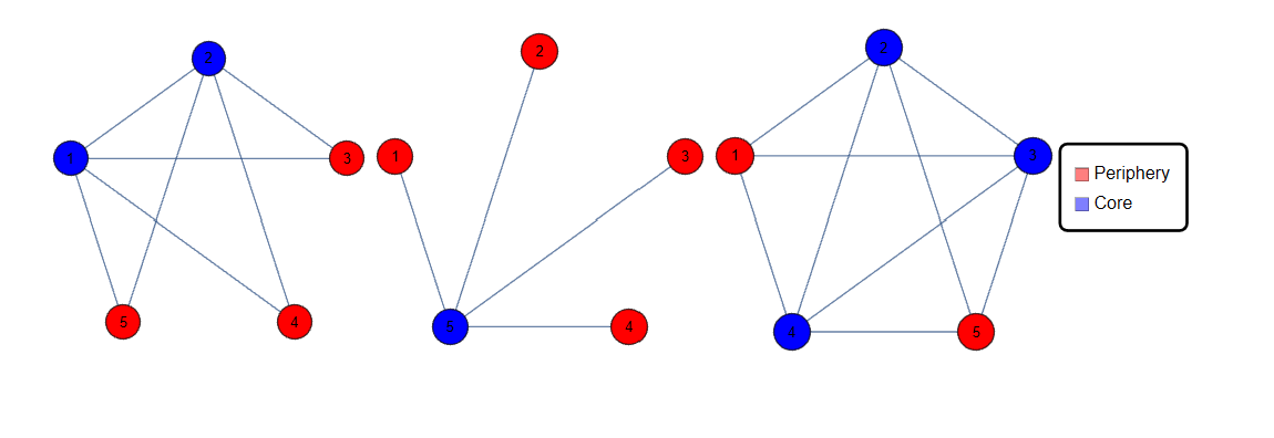
Figure 1: Examples of core-periphery networks on 5 vertices.

An important implication of our model is that whenever network participants lack information about the true architecture of the network, their behavior is not consistent with complete information behavior, nor with expectations over complete information equilibrium outcomes. This follows because equilibrium actions are determined by the interim expected sum of walks, which is different from the agent’s ex-ante expected walks (i.e., ex-ante expected Katz-Bonacich centrality). This finding speaks to a body of applied work that structurally estimates network effects in environments in which the architecture of the network is not known. A typical approach to incorporating such unknown network effects has been to do so via expectations over complete information network effects. Our result, however, suggests that the issue with such applied approaches is that they fail to internalize the fact that the subjects themselves may not know the network. Whenever this is the case, estimators of complete information network effects may not be informative as to the true behavior of the network system of interest.

Next, we show that the BNE of our game is not always monotonic in agents’ degrees. In other words, first order connectivity alone is insufficient to characterize global patterns of equilibrium behavior. The absence of monotonicity as a general equilibrium property is in sharp contrast with existing results in network games with incomplete information. For instance, the Bayesian Nash equilibria of Galleotti et al. (2010) as well as Jackson (2019) are both monotonic in agents’ degrees. Even though effort monotonicity in degrees does not always hold in our game, it emerges if we assume the ex-ante distribution to be uniform over all networks. Besides monotonicity, the equilibrium under uniformity exhibits two more properties that are typically imposed as assumptions in other models. The first is anonymity, which states that while agents are aware of the number of agents they are connected to, they are unaware of the identity of these adjacent agents. The second is independence, which states that the degree of any agent who is connected to another is independent of the latter’s degree.

Lastly, we consider a variation of our main model as a robustness check. Rather than assuming agents have beliefs over the network structure, we suppose they have beliefs over the links. This means that types are generated via a random network generation process instead of assuming that ex-ante beliefs are prescribed by a probability measure over the set of all graphs. Since the type space is maintained, the Harsanyi transformation of the linear quadratic game is preserved and thus, the system of best responses characterizing the BNE is also preserved. Therefore, even though the stochastic process generating types is of a different kind, the walk characterization of the equilibrium does not change.

Next, imposing independence in the generation links, we provide closed form characterizations of Bayesian-Nash equilibria when the formation process follows two well-known models. First, under Erdos-Renyi formation where all links are formed with equal probability, equilibrium effort levels are identical to those where beliefs are uniform over all networks. Therefore, the Erdos-Renyi generation process also gives rise to anonymity in equilibrium. Second, we consider homophilic linkage through a stochastic block generation process. Unlike the Erdos-Renyi process, homophilic linkage gives rise to a group identity property where agents weigh the complementarity strengths of their actions according to both intra and inter-group considerations.

To the best of our knowledge there have only been two other papers that introduce incomplete information into the model. De Marti and Zenou (2015) study a linear quadratic game of incomplete information in which agents lack information regarding model parameters other than the network itself. These include the link complementarity strength, and the return to own action. Unlike their work, we focus on incomplete information on the network. Closer to our model is the work of Breza, Chandrasekhar, and Tahbaz-Salehi (2018) who also employ a linear quadratic game in which agents lack complete information regarding the network itself. One of their crucial assumptions, however, is that the information set of any agent (i.e. the identity of their neighbors) doesn’t provide any information about their indirect connections. In other words, their expectations regarding the existence of links between their neighbors and other agents is independent of the information they are endowed with. As a result, their equilibrium gets mapped to agents’ ex-ante beliefs about the network. In contrast, we find that as long as agents are endowed with beliefs about network topology itself, local connectivity provides information regarding indirect connectivity and agents will make use of it towards equilibrium play. This local information being different for each player in turn, implies that the equilibrium is no longer mapped to their ex-ante beliefs about the network.

Other than the equilibrium characterization, our model provides an approach for studying incomplete information within the framework of the canonical linear quadratic network game. The model thus paves the way for the formal study of incomplete information variants of the plethora of applications of this game including aspects like intervention (Galeotti et al. (2020)) and endogenous network formation (Konig et al. (2014)) among others.

The rest of the paper is structured as follows. Section 2 contains tools from network theory that will be used throughout the paper and sets up the game. In section 3, we characterize its BNE and illustrate its computation. Section 4 discusses the relationship between degree monotonicity and equilibrium effort. Section 5 deals with random network generation. Section 6 concludes. All proofs as well as additional discussion on certain aspects of our model are relegated to the appendix.

2 Model

2.1 Preliminaries

Let $N=\{1,2,...,n\}$ denote the set of players. Letting $i\sim j$ denote a link between players $i$ and $j$, a network (or graph) $\mathbf{g}$ is the collection of all pairwise links that exist between the players. The links are undirected such that $i\sim j\in\mathbf{g}$ implies $j\sim i\in\mathbf{g}$. The network can be represented by its adjacency matrix which, with some abuse of notation, is also denoted as $\mathbf{g}=\left[g_{ij}\right]$, where $g_{ij}=1$ if a link exists between players $i$ and $j$, and $g_{ij}=0$ otherwise. There are no self-loops and thus $g_{ii}=0$ for all $i\in N$. We denote by $\mathit{\mathcal{G}_{n}}$ the set of all unweighted and undirected networks on $n$ vertices whose cardinality is $2^{\frac{n(n-1)}{2}}$.

Given the adjacency representation of a network $\mathbf{g}\in\mathit{\mathcal{G}_{n}}$ we let $\mathbf{g}_{i}$ denote its $i^{th}$ row. That is, $\mathbf{g}_{i}=(g_{i1},g_{i2},....,g_{in})\in\{0,1\}^{n}$, where it is understood that $g_{ii}=0$. In the following section, it will be convenient to represent any network $\mathbf{g}$ by the rows of its adjacency matrix:

$$\mathbf{g}^{T}=\left(\mathbf{g}_{1},\mathbf{g}_{2},..,\mathbf{g}_{n}\right)$$ (1)

Note that the fact that links are undirected implies $\mathbf{g}=\mathbf{g}^{T}$. The neighborhood of player $i$ is the set of players with whom $i$ is linked and is denoted by: $\mathbf{N}(\mathbf{g}_{i})=\{j:\text{ }g_{ij}=1\}$. The size of this set is $i$’s degree which counts the agent’s direct connections: $d(\mathbf{g}_{i})\equiv|\mathbf{N}(\mathbf{g}_{i})|$.

A walk of length $s$ from a node $i$ to a node $j_{s}$ is a sequence of links in the network $i\sim j_{1}$, $j_{1}\sim j_{2}$,…, $j_{s-1}\sim j_{s}$. It is denoted by $ij_{1}j_{2}...,j_{s}$. Given two nodes $i$ and $j_{s}$ there may exist more than one such walk. Using the adjacency representation, the number of walks of length $s$ from node $i$ to node $j_{s}$ can be computed by the $ij_{s}$ element of the matrix $\mathbf{g}^{s}$.

Finally, let $\mathbf{g}^{0}=\mathbf{I}$, then for a sufficiently small $\lambda>0$, the following influence matrix $\mathbf{M}(\mathbf{g}\mathbf{,}\lambda\mathbf{)=}\left[m_{ij}\left(\mathbf{g}\right)\right]$ is well-defined and non-negative:

$$\mathbf{M}(\mathbf{g},\lambda\mathbf{)\equiv}\left[\mathbf{I-}\lambda\mathbf{g}\right]^{-1}=\sum_{s=0}^{\infty}\lambda^{s}\mathbf{g}^{s}$$

Each element $m_{ij}\left(\mathbf{g}\right)$ measures the total number of walks of all lengths from agent $i$ to agent $j$. Given $\mathbf{M}(\mathbf{g}\mathbf{,}\lambda)$, the Katz-Bonacich (KB) centrality of player $i$, $b_{i}(\mathbf{g},\,\lambda)$, is the $i^{\text{th}}$-component of the vector $\boldsymbol{b}\left(\mathbf{g},\,\lambda\right)=\mathbf{M}(\mathbf{g},\lambda\mathbf{)1}_{n}$ where $\boldsymbol{1}_{n}$ is the n-dimensional column vector of ones. It measures the total number of discounted walks of all lengths originating from player $i$ to all other players in $\mathbf{g}$ where longer paths are discounted more.

2.2 The Game

We study a variant of the simultaneous move local complementarities game of Ballester et al. (2006), in which agents have incomplete information about the full architecture of the network.

We follow Harsanyi’s (1967) approach to games of incomplete information by introducing Nature as a non-strategic player who chooses a network out of a set containing all possible graphs on the number of vertices equal to the number of agents. The network is chosen from an ex-ante distribution that is common knowledge among all agents. Following Nature’s draw, players realize their direct connections (they can see the agents with whom they are linked), but do not know the network’s architecture beyond that. In other words, they do not observe the links of their neighbors. Using the information on their direct connections, agents proceed to update their beliefs about the network chosen by Nature according to Bayes’ rule. Given these updated beliefs, agents simultaneously exert actions to maximize their interim payoffs.

Agents and Types

$N$ is the set of players (nodes), with $\lvert N\rvert=n$. For each $i\in N$, we let $G_{i}$ denote the player’s type set. To incorporate information regarding direct connections, agents’ types are representative of their corresponding row in the adjacency representation of the network over which the game will be played. That is, each player’s type set assumes the following form:

$$G_{i}=\{(g_{i1},g_{i2},....,g_{in})_{i}\in\{0,1\}^{n}:g_{ii}=0\}$$

where $g_{ij}=1$ if player $i$ is connected to $j$ and 0 otherwise. Note that the outer subscript in $(g_{i1},g_{i2},....,g_{in})_{i}$ is imposed to differentiate between agents whose types consist of the same sequence of 0’s and 1’s. For instance, if $n=3$ it differentiates between the type $(0,1,0)_{1}$ for agent 1 and $(0,1,0)_{3}$ for agent 3. The first refers to agent 1’s links and the second to agent 3’s links. The cardinality of each agent’s type set is:

$$|G_{i}|\equiv\gamma=2^{n-1}$$

and we denote its elements by $\mathbf{g}_{i}^{t_{i}}\in G_{i}$. Whenever the context is clear and we need not enumerate the elements of each type set we suppress the superscript $t_{i}$. Given each player’s type set, we can write down the type space of the game:

$$G=\vartimes_{i\in N}G_{i}$$

Observe that if we invoke network representation (1), any element of $G$ may, or may not, correspond to the adjacency matrix of an undirected and unweighted network. That is, not all elements of $G$ have valid network representations. As an example, consider the case with 3 players, $N=\{1,2,3\}$. The type sets of the players are given by:

$$G_{1} =\{(0,0,0)_{1},(0,1,0)_{1},(0,0,1)_{1},(0,1,1)_{1}\}$$

$$G_{2} =\{(0,0,0)_{2},(1,0,0)_{2},(0,0,1)_{2},(1,0,1)_{2}\}$$

$$G_{3} =\{(0,0,0)_{3},(1,0,0)_{3},(0,1,0)_{3},(1,1,0)_{3}\}$$

with corresponding type space $G=G_{1}\times G_{2}\times G_{3}$. One element of $G$ is $((0,1,0)_{1}$, $(0,0,1)_{2}$, $(0,1,0)_{3})$. Observe that these entries do not correspond to rows of the adjacency matrix of an undirected and un-weighted network. According to this element, agent 1 is connected to agent 2 while agent 2 is not connected to agent 1. The corresponding adjacency matrix, therefore, would not symmetric. In this paper, we restrict attention to elements of $G$ that have valid representations so that Nature’s choice is reflective of an undirected and unweighted network. In what follows, we do so through the information structure.

Ex-Ante Beliefs

We denote by $p\in\Delta(G)$ the probability distribution over the type space, with $\Delta(G)$ denoting the set of all probability distributions over $G$. In our game, Nature moves first and chooses an element of the type space $\mathbf{g}\in G$. As noted above, we want to restrict Nature’s choice to those elements in $G$ that have valid network representations. Towards this, we define the following set of admissible distributions, and impose the assumption that Nature draws a network from a distribution in this set.

Definition 1.

We say that the probability distribution $p\in\Delta(G)$ is admissible if it satisfies:

$$p(\mathbf{g})=0,\text{ }\forall\text{ }\mathbf{g}\in G\text{ s.t. }\mathbf{g}\neq\mathbf{g}^{T},$$

and denote the set of all admissible distributions by $\Delta_{A}(G)$.

Assumption 1: $p\in\Delta_{A}(G)$ and this is common knowledge.

Observe that the imposition of assumption 1 implies that $p(\mathbf{g})\geq 0$ if and only if $\mathbf{g}\in\mathit{\mathcal{G}_{n}}$. Consequently, Nature will choose an unweighted and undirected network, and the fact that the agents are part of one such network is common knowledge.

As an example consider the uniform admissible distribution which is defined as follows:

Definition 2.

The probability distribution $p\in\Delta_{A}(G)$ is uniform if it satisfies:

$$p(\mathbf{g})=\begin{cases}\frac{1}{2^{\frac{n(n-1)}{2}}}&\text{if }\mathbf{g}\in\mathit{\mathcal{G}_{n}}\\ 0&\text{otherwise }\end{cases}$$

In the 3-player case, for instance, we have that $|\mathcal{G}_{3}|=8$ and Nature chooses any unweighted and undirected network with probability $p(\mathbf{g})=\frac{1}{8}$.

Belief Updating

Given assumption 1, agents know that Nature draws a network and proceed to update their beliefs regarding its true topology according to Bayes’ Rule. These updated updated beliefs can be written as:

$$p(\mathbf{g}_{j}|\mathbf{g}_{i})=\frac{p(\mathbf{g}_{i},\mathbf{g}_{j})}{p(\mathbf{g}_{i})}=\frac{\sum_{\mathbf{g}\in G}p(\mathbf{g})\mathbb{I}\{\mathbf{g}_{i}=\left.\mathbf{g}\right|_{i}\wedge\mathbf{g}_{j}=\left.\mathbf{g}\right|_{j}\}}{\sum_{\mathbf{g}\in G}p(\mathbf{g})\mathbb{I}\{\mathbf{g}_{i}=\left.\mathbf{g}\right|_{i}\}}\text{ }\forall i,j\in N,$$ (2)

where $\mathbb{I}$ is the indicator function. Specifically, for $\mathbf{g}\in G$, $\mathbb{I}\{\mathbf{g}_{i}=\left.\mathbf{g}\right|_{i}\}=1$ if $\mathbf{g}_{i}$ is the projection of $\mathbf{g}$ (i.e., $\left.\mathbf{g}\right|_{i}$ ) on its $i^{th}$ component and 0 otherwise. Intuitively, equation (2) states that agent $i$ who is of type $\mathbf{g}_{i}\in G_{i}$ will assign a probability to agent $j$ being of type $\mathbf{g}_{j}\in G_{j}$ according to (i) the number of states in the state space that contain both of these types, and (ii) the ex-ante probability that the agent’s own type is realized. Given assumption 1, since agent types correspond to rows of an adjacency matrix, the probability the agent $i$ (whose row is $\mathbf{g}_{i}$) will assign to an agent having a row $\mathbf{g}_{j}$ will depend on the number of networks that contain these rows, and the probability that nature selects them.

As an example, consider the 3-player case and suppose that after Nature’s draw, agent 2 is of type $(1,0,0)_{2}$. In other words, agent 2 learns that it is connected to agent 1 but is not connected to agent 3. Since players can only observe their neighbors, agent 2 does not know if agents 1 and 3 are themselves connected, and will thus have to form beliefs about the existence of a link between them. This is demonstrated in figure 2. However, the state space only contains 2 elements in which agent 2’s type is admissible with a valid network representation: $((0,1,0)_{1},\,(1,0,0)_{2},\,(0,0,0)_{3})$ and $((0,1,1)_{1},\,(1,0,0)_{2},\,(1,0,0)_{3})$. In other words, there are only two graphs on 3 vertices that contain the link $1\sim 2$ and do not contain the link $2\sim 3$. If we took the ex-ante distribution to be uniform, then agent 2 would assign a probability of $\frac{1}{2}$ that nature chose either of these.

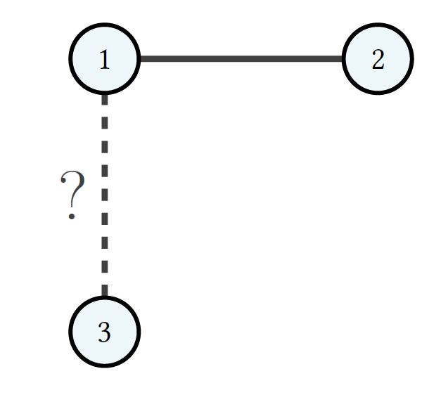
Figure 2: Representation of uncertainty for agent 2 whose type is $(1,0,0)_{2}$.

Note that assumption 1 implies that beliefs are consistent, in the sense that agents will assign zero probability to others being of types that do not match the adjacency pattern induced by their own type. This is expressed formally in the remark below.

Remark 1.

For all $g_{i}\in G_{i},\text{ }p(\mathbf{g}_{j}|\mathbf{g}_{i})=0\text{ }\forall\mathbf{g}_{j}\in G_{j}\text{ }\text{for which}\text{ }g_{ij}\neq g_{ji},\text{ }\forall i,j\in N.$

Lastly, we impose the following regularity assumption for conditioning on zero probability events.

Assumption 2: For any $\mathbf{g}_{j}\in G_{j}$, we set $p(\mathbf{g}_{j}|\mathbf{g}_{i})=0$, for all $\mathbf{g}_{i}\in G_{i}$ for which $p(\mathbf{g}_{i})=0$, $\forall i,j\in N$

In words, assumption 2 states that agents will assign zero probability to any type whenever its conditioned on another whose marginal probability is zero under the prior. This assumption is solely imposed for ease of notation and allows us to place zero probability mass that Nature selects specific sets of networks in examples that follow. In particular, whenever ex-ante beliefs place zero probability on specific elements of the type space being realized, Bayes rule for certain updates becomes ill defined. To avoid this issue while still disallowing for certain networks to be drawn by Nature, agents’ type sets and corresponding type spaces must be redefined on a full support. Nature would place a strictly positive probability on all networks of interest, while networks that would be assigned a zero probability measure under the current prior are excluded from the type space. We demonstrate this construction formally in appendix C, where we also show that this approach produces the same equilibrium as the one generated without altering the type space while imposing assumption 2.

State Game and Equilibrium

Given the above, conditional on a state $\mathbf{g}\in G$ being realized, agents play the state game:

$$s_{\mathbf{g}}=(N,A,(u_{i}(\mathbf{a}_{i},\text{ }\mathbf{a}_{-i}))_{i\in N})$$

where every agent has the same action set $A\equiv\mathbb{R}_{+}$. Let $\mathbf{a}_{j}=(a_{j}(\mathbf{g}_{j}^{1}),...,a_{j}(\mathbf{g}_{j}^{\gamma}))$ , $\mathbf{a}_{-i}=(\mathbf{a}_{1},...,\mathbf{a}_{i-1},\mathbf{a}_{i+1},...,\mathbf{a}_{n})$ and $\mathbf{a}_{i}(\mathbf{g}_{i}^{-t_{i}})=(a_{i}(\mathbf{g}_{i}^{1}),...,a_{i}(\mathbf{g}_{i}^{t_{i}-1}),a_{i}(\mathbf{g}_{i}^{t_{i}+1}),...,a_{i}(\mathbf{g}_{i}^{\gamma}))$. Interim utilities assume a linear-quadratic form:

$$u_{i}(a_{i}(\mathbf{g}_{i}^{t_{i}});\text{ }\mathbf{a}_{i}(\mathbf{g}_{i}^{-t_{i}}),\text{ }\mathbf{a}_{-i})=a_{i}(\mathbf{g}_{i}^{t_{i}})-\frac{1}{2}a_{i}(\mathbf{g}_{i}^{t_{i}})^{2}+\lambda a_{i}(\mathbf{g}_{i}^{t_{i}})\sum_{j=1}^{n}g_{ij}^{t_{i}}\sum_{\mathbf{g}_{j}\in G_{j}}p(\mathbf{g}_{j}|\mathbf{g}_{i}^{t_{i}})a_{j}(\mathbf{g}_{j})$$ (3)

As in Ballester et al. (2006) the first two terms in the utility specification capture the direct benefit and cost to agent $i$ from exerting its own action. The third term captures local complementarities with those agents that the player is connected to, with $\lambda$ measuring the strength of this complementarity. Note, however, that unlike the complete information set up of Ballester et al. (2006), agents need to form beliefs about the actions of their neighbors.

Agents simultaneously exert actions to maximize (3). For each agent $i$, a pure strategy $\sigma_{i}$ maps each possible type to an action. That is,

$$\sigma_{i}=(a_{i}(\mathbf{g}_{i}^{1}),...,a_{i}(\mathbf{g}_{i}^{\gamma}))$$

This is a simultaneous move game of incomplete information so we invoke Bayes-Nash as the equilibrium notion.

Definition 3.

The pure strategy profile $\sigma^{*}=(\sigma_{i}^{*},\text{ }\sigma_{-i}^{*})$ where $\sigma_{i}=(a_{i}^{*}(\mathbf{g}_{i}^{1}),...,a_{i}^{*}(\mathbf{g}_{i}^{\gamma}))$ is a Bayesian-Nash equilibrium (BNE) if:

$$a_{i}^{*}(\mathbf{g}_{i}^{t_{i}})=arg\text{ }\underset{a_{i}(\mathbf{g}_{i}^{t_{i}})}{max}\text{ }u_{i}(a_{i}(\mathbf{g}_{i}^{t_{i}}),\text{ }\mathbf{a}_{i}^{*}(\mathbf{g}_{i}^{-t_{i}}),\text{ }\mathbf{\sigma}_{-i}^{*})\text{ }\forall\text{ }i\in N,\text{ }\forall\text{ }\mathbf{g}_{i}^{t_{i}}\in G_{i}$$

The above game can be summarized according to the tuple:

$$\boldsymbol{\Gamma}=\left<N,(G_{i})_{i\in N},p,(s_{\mathbf{g}})_{\mathbf{g}\in G}\right>$$ (4)

3 Bayesian Nash Equilibrium

We now characterize the BNE of $\mathbf{\boldsymbol{\Gamma}}$ starting with best responses.

3.1 Best Responses

Given the payoff structure, the best response of the $i^{th}$ player who is of type $\mathbf{g}_{i}^{t_{i}}$ is given by:

$$a_{i}(\mathbf{g}_{i}^{t_{i}})=1+\lambda\sum_{j=1}^{n}g_{ij}^{t_{i}}\sum_{\mathbf{g}_{j}\in G_{j}}p(\mathbf{g}_{j}|\mathbf{g}_{i}^{t_{i}})a_{j}(\mathbf{g}_{j})$$

The system characterizing the best responses for all players can be written in vector notation as follows:

$$\mathbf{a}=\mathbf{1}_{n\gamma}+\lambda\mathbb{B}\mathbf{a}$$ (5)

where $\mathbf{1}_{n\gamma}$ is the $n\gamma$-dimesnional column vector of 1’s, $\mathbf{a}=\left[\mathbf{a}_{i}\right]_{i=1}^{n}$ , $\mathbf{a}_{i}=\left[a_{i}(\mathbf{g}_{i}^{t_{i}})\right]_{t_{i}=1}^{\gamma}$, $\gamma=2^{n-1}$ is the total number of types of each player, and $\mathbb{B}$ is a block matrix that assumes the following form:

$$\mathbb{B}=\begin{pmatrix}\mathbf{0}&G_{1\sim 2}&\ldots&G_{1\sim n}\\ G_{2\sim 1}&\mathbf{0}&\ldots&G_{2\sim n}\\ \ldots&\ldots&\ldots&\ldots\\ G_{n\sim 1}&G_{n\sim 2}&\ldots&\mathbf{0}\end{pmatrix}_{n\gamma\times n\gamma}$$

with

$$\left[G_{i\sim j}\right]_{t_{i}t_{j}}=g_{ij}^{t_{i}}p(\mathbf{g}_{j}^{t_{j}}|\mathbf{g}_{i}^{t_{i}})\quad\forall\text{ }t_{j},t_{i}=1,..,\gamma\quad\text{and}\quad\forall\text{ }\mathbf{g}_{j}^{t_{j}}\in G_{j},\mathbf{g}_{i}^{t_{i}}\in G_{i}$$

It can be verified that if the ex-ante distribution satisfies $p(\mathbf{g})=1$ for a specific $\mathbf{g}\in\mathcal{G}_{n}$ and $p(\mathbf{g}^{\prime})=0$ for all $\mathbf{g}^{\prime}\neq\mathbf{g}$, then $a_{i}(\mathbf{g}_{i})=0$ for all $i\in N$ for which $\mathbf{g}_{i}\notin\mathbf{g}$. For this case, the system of best responses would reduce to the one that characterizes the complete information Nash equilibrium (Ballester et al. (2006)):

$$\mathbf{a}^{c}=\mathbf{1}_{n}+\lambda\mathbf{g}\mathbf{a}^{c}$$ (6)

where $\mathbf{a}^{c}=(a_{1}(\mathbf{g}_{1}),..,a_{n}(\mathbf{g}_{n}))$ and $\mathbf{g}=(\mathbf{g}_{1},..,\mathbf{g}_{n})$. In other words, in the complete information case, the matrix $\mathbf{\mathbb{B}}$ would reduce to the actual network over which the game is played, and agents would best respond to the actions of their adjacent agents. In the incomplete information case, however, agents do not know the types of their neighbors and best respond to updated beliefs regarding their actions. This is captured by the elements within the blocks of $\mathbf{\mathbb{B}}$. For instance, consider agent $i$ and the block $\left[G_{i\sim j}\right]_{t_{i}t_{j}}$. Its elements are of the form $g_{ij}^{t_{i}}p(\mathbf{g}_{j}^{t_{j}}|\mathbf{g}_{i}^{t_{i}})$, which states that if agent $i$ whose type $\mathbf{g}_{i}^{t_{i}}$ is such that it is connected to agent $j$, to this agent it will assign the probability being of type $\mathbf{g}_{j}^{t_{j}}$ equal to $p(\mathbf{g}_{j}^{t_{j}}|\mathbf{g}_{i}^{t_{i}})$. Observe, that such beliefs are not needed in the complete information case. Moreover, this updating affects equilibrium outcomes if and only if agent $i$ is connected to agent $j$, which may be interpreted as saying that agents form beliefs about others if and only if a link exists between them. In this sense, the matrix $\mathbb{B}$ may be interpreted in a similar fashion to the complete information case, but instead of adjacency over agents, it provides the adjacency pattern over all network admissible types. In turn, this gives rise to a network between the types themselves.

To illustrate, suppose that $n=3$ and let the underlying distribution be uniform on $\mathit{\mathcal{G}_{3}}$. In this case, updated beliefs are given by $p(\mathbf{g}_{j}|\mathbf{g}_{i})=\frac{1}{2},\forall\mathbf{g}_{j}\in G_{j}$ so that the vector of actions and the matrix $\mathbb{B}$ assume the following form:

$$\mathbf{a}=\begin{bmatrix}a_{1}((0,0,0)_{1})\\ a_{1}((0,1,0)_{1})\\ a_{1}((0,0,1)_{1})\\ a_{1}((0,1,1)_{1})\\ -\\ a_{2}((0,0,0)_{2})\\ a_{2}((1,0,0)_{2})\\ a_{2}((0,0,1)_{2})\\ a_{2}((1,0,1)_{2})\\ -\\ a_{3}((0,0,0)_{3})\\ a_{3}((1,0,0)_{3})\\ a_{3}((0,1,0)_{3})\\ a_{3}((1,1,0)_{3})\end{bmatrix}\quad\mathbb{B}=\frac{1}{2}\left(\begin{array}[]{cccccccccccccc}0&0&0&0&|&0&0&0&0&|&0&0&0&0\\ 0&0&0&0&|&0&1&0&1&|&0&0&0&0\\ 0&0&0&0&|&0&0&0&0&|&0&1&0&1\\ 0&0&0&0&|&0&1&0&1&|&0&1&0&1\\ -&-&-&-&-&-&-&-&-&-&-&-&-&-\\ 0&0&0&0&|&0&0&0&0&|&0&0&0&0\\ 0&1&0&1&|&0&0&0&0&|&0&0&0&0\\ 0&0&0&0&|&0&0&0&0&|&0&0&1&1\\ 0&1&0&1&|&0&0&0&0&|&0&0&1&1\\ -&-&-&-&-&-&-&-&-&-&-&-&-&-\\ 0&0&0&0&|&0&0&0&0&|&0&0&0&0\\ 0&0&1&1&|&0&0&0&0&|&0&0&0&0\\ 0&0&0&0&|&0&0&1&1&|&0&0&0&0\\ 0&0&1&1&|&0&0&1&1&|&0&0&0&0\end{array}\right)$$

Consider player 2 and suppose it has realized the type $(1,0,0)_{2}$ (as visualized in figure 2). The player knows that it is connected to player 1, as $g_{21}=1$, and that it is not connected to 3, as $g_{23}=0$. Therefore, agent 2 will form beliefs over agent 1’s types. Since the only types of agent 1 that are network admissible with the type $(1,0,0)_{2}$ are $(0,1,1)_{1}$ and $(0,1,0)_{1}$, then there exists a link between the types $(1,0,0)_{2}$ and $(0,1,1)_{1}$ as well as between $(1,0,0)_{2}$ and $(0,1,0)_{1}$. A similar argument holds for all other agents and all of their possible types. Therefore, we may think of $\mathbb{B}$ as an adjacency matrix whose entries are representative of links between network admissible types. For this three player example, the network is shown in figure 3.

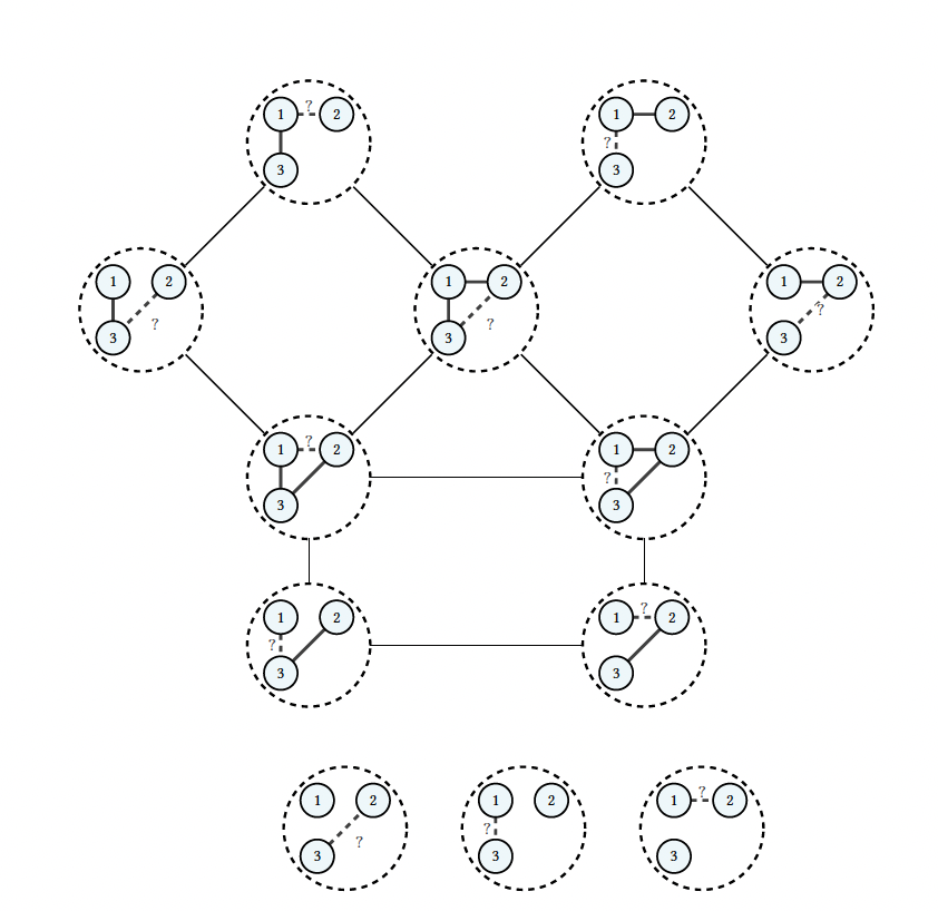
Figure 3: Network between types of each players

Before we proceed, we note that closest to our best response characterization is the interaction structure considered in Golub and Morris (2020). Although the signal realizations of each agent in their model can be thought of as arising from a more general information structure (which could potentially allow for network signals themselves), the network architecture itself is nonetheless common knowledge. In their general theory of networks and information, agent behavior is driven by an endowed interaction structure similar to our matrix $\mathbb{B}$. In our model, however, this is generated endogenously as a result of optimizing behavior.

3.2 Existence-Uniqueness

According to definition 3, the BNE is characterized by the fixed point of the system of equations in (5). We have the following classification:

Theorem 1.

There exists a unique pure strategy BNE for $\lambda\in\left[0,\frac{1}{n-1}\right)$.

Observe that the bound on the local complementarity parameter $\lambda$ which guarantees the existence and uniqueness of an equilibrium is identical to the complete information bound. Algebraically, this holds because the elements in each row of $\mathbb{B}$ sum to at most $n-1$. This can be seen from the fact that the non-zero rows of its blocks $\left[G_{i\sim j}\right]_{kl}$ sum to 1, as they correspond to conditional probability distributions over network admissible types.

The linear quadratic game played on networks is about direct and indirect complementarities. Intuitively, $n-1$ represents the maximal number of agents that each individual can extract direct complementarities from. Since the complementarity strength arising from a single link is $\lambda$, the maximal direct complementarity that may be extracted by a single agent is $\lambda(n-1)$. Moreover, agents are embedded in a network, so they can also extract complementarities from their indirect connections. In the complete information case, the maximal complementarity that can be extracted by a single agent due to their $s^{th}$ order indirect connections is $\lambda^{s}(n-1)^{s}$. Therefore, summing over all $s\in\mathbb{N}_{+}$ gives the maximal complementarity that any agent can extract from any network. This, in turn, provides a bound on the strength of $\lambda$ for actions to be bounded.

Now in the incomplete information case, a similar argument holds, but the bound on the maximal complementarity that may be extracted from the network is attained by decomposing it across states rather than links. For example, consider an agent $i$ who is of type $\mathbf{g}_{i}$, and who is connected to agent $j$. Given updated beliefs, agent $i$ assigns a probability $p(\mathbf{g}_{j}|\mathbf{g}_{i})$ to agent $j$ being of type $\mathbf{g}_{j}$. This in turn induces a complementarity strength of $\lambda p(\mathbf{g}_{j}|\mathbf{g}_{i})$ between the action of agent $i$ and that of an agent $j$ who is of the particular type $\mathbf{g}_{j}$. Since $\sum_{g_{j}\in G_{j}}p(\mathbf{g}_{j}|\mathbf{g}_{i})=1$, then the maximal complementarity that can be extracted from a single neighbor is $\lambda$. A similar argument holds for indirect connections. In other words, the complementarity an agent $i$ extracts from another $j$, is spread out across all of $j^{\prime}s$ types that are admissible with the realized type of agent $i$. In this sense, the model generates network externalities on the agent-state specific level rather than the agent specific level. This has important consequences for the nature of the BNE. We turn to its characterization next.

3.3 Walk Characterization

Recall that $a_{i}^{*}(\mathbf{g}_{i}^{t_{i}})$ denotes the equilibrium action of agent $i$ whose realized type is $\mathbf{g}_{i}^{t_{i}}\in G_{i}$. The following theorem characterizes the BNE for any ex-ante distribution and any realized network.

Theorem 2.

For any $s\in\mathbb{N}_{+}$ let $j_{1},j_{2},..,j_{s}$ denote an arbitrary collection of $s$ indices. For any admissible probability distribution, and for any realized network $\mathbf{g}\in G$, the equilibrium actions of agents are given by:

$$a_{i}^{*}(\mathbf{g}_{i}^{t_{i}})=\sum_{s=0}^{\infty}\lambda^{s}\beta_{i,t_{i}}^{(s)}\quad\forall\text{ }i\in N,\text{ }\forall\text{ }\mathbf{g}_{i}^{t_{i}}\in G_{i}$$

where $\mathbf{g}_{i}^{t_{i}}=(g_{ij}^{t_{i}})_{j\in N}$ is the realized type of agent $i$, and where:

$$\beta_{i,t_{i}}^{(s)}=\sum_{j_{1},j_{2},..,j_{s}=1}^{n}\text{ }\sum_{t_{j_{1}},t_{j_{2}},..,t_{j_{s-1}}=1}^{\gamma}g_{ij_{1}}^{t_{i}}g_{j_{1}j_{2}}^{t_{j_{1}}}...g_{j_{s-1}j_{s}}^{t_{j_{s-1}}}p(\mathbf{g}_{j_{s-1}}^{t_{j_{s-1}}}|\mathbf{g}_{j_{s-2}}^{t_{j_{s-2}}})p(\mathbf{g}_{j_{s-2}}^{t_{j_{s-2}}}|\mathbf{g}_{j_{s-3}}^{t_{j_{s-3}}})...p(\mathbf{g}_{j_{1}}^{t_{j_{1}}}|\mathbf{g}_{i}^{t_{i}})$$

Theorem 2 is best understood when compared to the complete information Nash equilibrium over the same network:

$$a_{i}^{c}(\mathbf{g}_{i}^{t_{i}})=\sum_{s=0}^{\infty}\lambda^{s}\left[\sum_{j_{1},j_{2},..,j_{s}=1}^{n}g_{ij_{1}}^{t_{i}}g_{j_{1}j_{2}}^{t_{j_{1}}}...g_{j_{s-1}j_{s}}^{t_{j_{s-1}}}\right]\equiv\sum_{s=0}^{\infty}\lambda^{s}d_{i}^{(s)}=b_{i}\left(\mathbf{g},\,\lambda\right)$$

For each $s\in\mathbb{N}_{+}$, $d_{i}^{(s)}$ measures the total number of length $s$ walks originating from player $i$ to all others (including $i$ itself). In the complete information scenario, each agent has knowledge of the full architecture of the network and can thus compute these walks for all lengths $s$. Intuitively, each of these walks $ij_{1}j_{2},..,j_{s}$, captures the complementarity of agent $i^{\prime}s$ action with that of agent $j_{s}$ due to the existence of a particular sequence of intermediate links $i\sim j_{1}$, $j_{1}\sim j_{2}$,.., $j_{s-1}\sim j_{s}$ connecting them. Thus, each agent will take into account all of these complementarities and exert an action equal to their total strength. In turn, this produces Nash equilibrium effort levels equal to the agents’ KB centralities.

In the incomplete information case, knowledge of these walks is limited to those that are of first order, as agents can only identify their neighbors. Even though information is limited, agents are nonetheless aware of the fact that they participate in a network, and hence, internalize the fact that walks of arbitrary orders may exist between them and all other agents. Since these walks capture complementarity strengths, that in turn dictate the magnitude of actions, agents will need to form expectations as to what their actual strength is. In the statement of theorem 2, each term $\lambda^{s}\beta_{i,t_{i}}^{(s)}$ captures this expected measure for all walks of the particular order $s$.

To describe this expected measure in more detail, consider the case $s=3$. With a slight rearrangement of terms we can write

$$\beta_{i,t_{i}}^{(3)} =\sum_{j,k,l=1}^{n}\sum_{t_{j},t_{k}=1}^{\gamma}g_{ij}^{t_{i}}g_{jk}^{t_{j}}g_{kl}^{t_{k}}p(\mathbf{g}_{k}^{t_{k}}|\mathbf{g}_{j}^{t_{j}})p(\mathbf{g}_{j}^{t_{j}}|\mathbf{g}_{i}^{t_{i}})$$

$$=\sum_{j,k=1}^{n}\sum_{l=1}^{n}g_{ij}^{t_{i}}\sum_{t_{j}=1}^{\gamma}g_{jk}^{t_{j}}p(\mathbf{g}_{j}^{t_{j}}|\mathbf{g}_{i}^{t_{i}})\sum_{t_{k}=1}^{\gamma}g_{kl}^{t_{k}}p(\mathbf{g}_{k}^{t_{k}}|\mathbf{g}_{j}^{t_{j}})$$

As per the timing of events in the game, agent $i$ gets to know its type $\mathbf{g}_{i}^{t_{i}}$, and hence has full knowledge of the links $g_{ij}^{t_{i}}$. The player is, therefore, aware of the agents through which it can form a walk of length three. To fix ideas, suppose that player $i$ wants to form a belief about the complementarity strength of its action with that of agent $l$ due to the particular walk $ijkl$. Recall that agent $i$ has complete information about $g_{ij}^{t_{i}}$, i.e. the link between it and agent $j$. However, it does not have complete information about $j^{\prime}s$ type, nor about $j^{\prime}s$ neighbors’ neighbors’ type which in turn may or may not include a link with agent $k$ through which the walk of interest $ijkl$ reaches agent $l$.

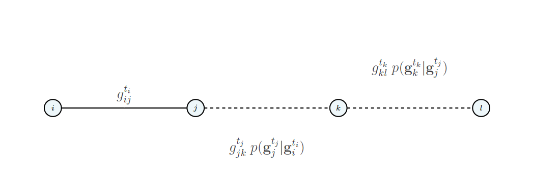
Figure 4: Expected walk of length 3

The expectation regarding the strength of this complementarity is formed in three steps. First, the agent will condition on the fact that it has a link with agent $j$. This occurs with probability $p(\mathbf{g}_{i}^{t_{i}}|\mathbf{g}_{i}^{t_{i}})=1$ (since we are assuming that $g_{ij}^{t_{i}}=1$) and thus, we may think of $g_{ij}^{t_{i}}$ as the expected number of ways that agent $i$ can reach agent $j$. Second, the agent internalizes its own type through $p(\mathbf{g}_{j}^{t_{j}}|\mathbf{g}_{i}^{t_{i}})$, to compute expectations over the links between its neighbor $j$ and its neighbors’ neighbor $k$. Using this, the agent counts the expected number of ways it can reach $k$ through $j$, conditional on the existence of the link $g_{ij}^{t_{i}}$. This is given by $\sum_{t_{j}=1}^{\gamma}g_{jk}^{t_{j}}p(\mathbf{g}_{j}^{t_{j}}|\mathbf{g}_{i}^{t_{i}})$. Third, the agent internalizes the information about the possible types of its neighbor $j$ through $p(\mathbf{g}_{k}^{t_{k}}|\mathbf{g}_{j}^{t_{j}})$, to compute the expectations over the links between its neighbors’ neighbor $k$ and agent $l$, (who is its neighbors’ neighbors’ neighbor). Using this, the agent counts the expected number of possible ways it can reach $l$ through $k$, conditional on the existence of the link $g_{jk}^{t_{j}}$. This is given by $\sum_{t_{k}=1}^{\gamma}g_{kl}^{t_{k}}p(\mathbf{g}_{k}^{t_{k}}|\mathbf{g}_{j}^{t_{j}})$.

Given the above, the expected total number of ways player $i$ can reach player $l$ via a walk of length three is given by the product of (i) the actual link between it and $j$, (ii) the number of ways it can reach $k$ from $j$ given the previous link $g_{ij}^{t_{i}}$ exists and (iii) the number of ways it can reach $l$ from $k$ given $g_{jk}^{t_{j}}$ exists. Repeating this process for all possible walks of length three which start from agent $i$, summing over all possible values of $j,k$ and $l$, and multiplying by $\lambda^{3}$, gives the expected complementarity strength of agent $i^{\prime}s$ action with all other agents due to walks of length three, $\lambda^{3}\beta_{i,t_{i}}^{(3)}$.

There are a couple of remarks that we make with regard to the nature of the preceding expected complementarity calculation.

Remark 2.

$\beta_{i,t_{i}}^{(s)}\neq\mathbb{E}\left(d_{i}^{(s)}\right)$

This remark states that the expected complementarity arising from walks of length $s$ does not equal its ex-ante expected value. This is not surprising, since the equilibrium is an interim notion which allows for belief-updating. An important consequence of this, nonetheless, is that the BNE equilibrium of this game does not equal the ex-ante expectation of KB centrality.

Motivated by complete information equilibrium notions, applied work has proposed estimators of network effects in environments in which researchers cannot observe the network. These approaches implicitly presume that although the researcher does not have information about the network, the agents themselves do. In other words, the data generating process is presumed to arise from network interactions under complete information. The proposed estimators are reflective of this, as they correspond to ex-ante expectations of complete information outcomes. As demonstrated by Breza et al. (2018), however, the assumption that a researcher is unaware of the network while the subjects are aware of it, may in some cases be inconsistent. If so, and as Proposition 2 suggests, agent behavior under such information settings would not correspond to ex-ante expectations over complete information outcomes.

Remark 3.

$\beta_{i,t_{i}}^{(s)}\neq\mathbb{E}\left(d_{i}^{(s)}|\;\mathbf{g}_{i}^{t_{i}}\right)$

To shed more light on this, consider the case of $s=3$.

$$\mathbb{E}\left(d_{i}^{(3)}|\;\mathbf{g}_{i}^{t_{i}}\right) =\mathbb{E}\left(\sum_{j,k=1}^{n}\sum_{l=1}^{n}g_{ij}g_{jk}g_{kl}\;|\;\mathbf{g}_{i}^{t_{i}}\right)$$

$$=\sum_{j,k=1}^{n}\sum_{l=1}^{n}\mathbb{E}\left(g_{ij}g_{jk}g_{kl}\;|\;\mathbf{g}_{i}^{t_{i}}\right)$$

$$=\sum_{j,k=1}^{n}\sum_{l=1}^{n}\sum_{t_{j}=1}^{\gamma}\sum_{t_{k}=1}^{\gamma}g_{ij}^{t_{i}}g_{jk}^{t_{j}}g_{kl}^{t_{k}}p\left(g_{jk}^{t_{j}}g_{kl}^{t_{k}}\;|\;\mathbf{g}_{i}^{t_{i}}\right)$$

This hypothetical interim expectation calculation fails to capture the process through which the agent $i$ internalizes the possible types of its neighbors, its neighbors’ neighbors and so on. In other words, only conditioning on its own type $\mathbf{g}_{i}^{t_{i}}$ makes it a more restricted measure. On the other hand, $\beta_{i,t_{i}}^{(s)}$ gives us the process by which agent $i$ internalizes the possible types of all agents on arbitrary walks starting from the agent.

3.4 A Core-Periphery Example

To illustrate the disparity between the complete information Nash equilibrium and incomplete information BNEs, we consider a special class of networks that are quite popular in the networks literature and allow for closed form characterizations.

Definition 4.

Let $n_{co}\in\{0,...,\,n-2\}\cup\{n\}$ and $n_{p}=n-n_{co}$. The adjacency matrix of a core-periphery network assumes the following form:

$$\mathbf{g}^{cp}=\begin{pmatrix}\mathbf{g}_{n_{co}}^{c}&\boldsymbol{1}_{n_{co}\times n_{p}}\\ \boldsymbol{1}_{n_{p}\times n_{co}}&\boldsymbol{0}_{n_{p}\times n_{p}}\end{pmatrix}$$

where $\mathbf{g}_{n_{q}}^{c}$ denotes the adjacency matrix of the complete network on $n_{q}$ vertices, and $\boldsymbol{1}_{n_{k}\times n_{s}}$ and $\boldsymbol{0}_{n_{k}\times n_{s}}$ respectively denote the $n_{k}\times n_{s}$ matrices of ones and zeros.

In words, a network has a core-periphery architecture if it consists of $n_{co}$ vertices that are connected to all others called the core, and $n_{p}=n-n_{co}$ vertices that are only connected to the core called the periphery. The star ($n_{co}=1$), the empty $(n_{co}=0)$, and the complete network ($n_{co}=n$) are special cases of core-periphery networks.

Under complete information, symmetry in network position induces symmetric best responses implying that all core agents incur an identical effort level and all peripheral agents also incur an identical effort level. Letting $a_{co}^{c}$ and $a_{p}^{c}$ denote these complete information Nash equilibrium actions of a core and a peripheral player respectively, it can be shown that:

$$a_{co}^{c} =\frac{1+\lambda n_{p}}{1-\lambda(n_{co}-1)-\lambda^{2}n_{p}n_{co}}$$

$$a_{p}^{c} =1+\lambda n_{co}a_{co}^{c}$$

To compare this complete information Nash equilibrium with an incomplete information BNE in which this particular type of network structure has a critical function, we endow individuals with the ex-ante belief that the actual network over which the game is played has a core-periphery architecture. Moreover, we assume that any such network is equally likely to be selected by Nature. Formally, let $\mathcal{G}_{n}^{CP}\subset\mathcal{G}_{n}$ be the collection of all possible core-periphery networks on $n$ vertices whose cardinality is $|\mathcal{G}_{n}^{CP}|=2^{n}-(n-1)$. Then, these ex-ante beliefs can be written as follows:

$$p_{cp}(\mathbf{g})=\begin{cases}\frac{1}{|\mathcal{G}_{n}^{CP}|}&\text{if}\,\mathbf{g}\in\mathcal{G}_{n}^{CP}\\ 0&\text{otherwise}\end{cases}$$

Observe that if Nature selects a graph according to this distribution, the type of an arbitrary player $\mathbf{g}_{i}^{t_{i}}$ can fall in one of two categories. Either $\sum_{i}g_{ij}^{t_{i}}=n-1$ in which case the agent knows it is the core, or $\sum_{i}g_{ij}^{t_{i}}=n_{co}<n-1$ where it realizes it is in the periphery. Since players observe the identity of their neighbors, and they know that Nature draws some core-periphery network with certainty, an individual who realizes it is in the periphery is able to infer the architecture of the entire network. On the other hand, when an individual realizes it is in the core it does not know whether its neighbors are core or peripheral players. This information structure, together with the fact that all core-periphery networks are equally likely to be chosen by Nature, leads to the following characterization.

Proposition 1.

Suppose $p=p_{cp}$ over $n>3$ vertices and that nature has chosen a core-periphery network with $n_{co}$ core nodes and $n_{p}$ peripheral nodes. Let $a_{co_{i}}^{*}$ denote the equilibrium action of agent $i$ who has realized that it is in the core, and $a_{p}^{*}$ the equilibrium action of a peripheral agent. Then, the BNE is given by

$$a_{co_{i}}^{*} =\frac{1+\lambda\mathbb{E}_{i}\left[n_{p}\right]}{1-\lambda\mathbb{E}_{i}\left[n_{co}-1\right]-\lambda^{2}\mathbb{E}_{i}\left[n_{p}n_{co}\right]}$$

$$a_{p}^{*} =1+\lambda n_{co}a_{co}^{*}$$

where

$$\mathbb{E}_{i}\left[n_{p}\right]=(n-1)\frac{\sum_{k=1}^{n-2}\binom{n-2}{k-1}}{2^{n-1}-(n-1)},\quad\mathbb{E}_{i}\left[n_{p}n_{co}\right]=(n-1)\frac{\sum_{k=1}^{n-2}k\binom{n-2}{k-1}}{2^{n-1}-(n-1)},$$

$$\mathbb{E}_{i}\left[n_{co}-1\right]=(n-1)\frac{\sum_{k=2}^{n}\binom{n-2}{k-2}-\binom{n-2}{n-3}}{2^{n-1}-(n-1)}$$

Observe that the functional form of the BNE is identical to the complete information Nash equilibrium. This is a consequence of the fact that when all the probability mass is distributed over core-periphery networks, an agent who realizes it is in the core is able to infer that the types of walks that it has in the network are identical to those it would have under complete information. Examples of these walks include walks from the core to the core via the core, walks from the core to the periphery via the core, etc. While walk types of a core agent are the same as the complete information case, the agent cannot infer the actual number of walks that it has. Nonetheless, the uniform assumption implies that any two walks of a particular type provide the same complementarity strength. This in turn leads to the characterization in Proposition 1.

With regard to peripheral agents, even though they know the architecture of the entire network (and hence the actual number of walks they have in the network), they do no exert $a_{p}^{c}$ in equilibrium. This is because they internalize that core agents cannot infer the topology of the entire network themselves. Consequently, a peripheral agent conditions upon the fact that core agents will exert $a_{co_{i}}^{*}$ in equilibrium, and exerts an action which is equal to the actual complementarity it is able to extract from the network i.e., $1+\lambda n_{co}a_{co_{i}}^{*}$.

Finally, unlike the complete information case where equilibrium actions of core and peripheral agents are strictly increasing with the size of the core, incomplete information actions do not change with the network realization. The following Lemma shows that whenever the size of the core is below half the population size, agents over-exert actions relative to the complete information Nash equilibrium.

Lemma 1.

For any core-periphery network on $n\geq 7$ vertices, if the size of the core satisfies $n_{co}\leq n/2$, then $a_{co}^{c}<a_{co_{i}}^{*}$.

As a corollary, it also follows that when the core size is below half the population size, incomplete information action levels are closer to the first best. Under complete information, efficient actions solve the welfare maximization problem. As shown by Belhaj, Bervoets and Deroian (2016), with linear quadratic utility over any network $\mathbf{g}$ and link complementarity strength $\lambda$, the efficient action level of player $i$ is given by $a_{i}^{e}=\boldsymbol{b}\left(\mathbf{g},\,2\lambda\right)$ which is strictly greater than the Nash equilibrium level $a_{i}^{c}=\boldsymbol{b}\left(\mathbf{g},\,\lambda\right)$.

Corollary 1.

For any core-periphery network on $n\geq 7$ vertices, if the size of the core satisfies $n_{co}\leq n/2$, then $a_{co}^{c}<a_{co_{i}}^{*}<a_{co}^{e}$ . If $n_{co}>\frac{n}{2}$, then $a_{co_{i}}^{*}<a_{co}^{c}<a_{co}^{e}$. Similarly for peripheral agents.

Apart from closed-form comparisons between complete and incomplete information equilibria, this core-periphery example highlights the interplay between private information and strategic behavior in network games with local complementarity. In particular, our results in this section allude to two conflicting intuitions that concord under the basis of strategic behavior. To illustrate further, we first note that the core-periphery networks belong to a larger class of networks known as nested split graphs (NSGs). These networks are representative of connection hierarchies (Konig et al. (2014)), consisting of agents whose neighborhood sets are nested. That is, agents are only linked to others who are in turn at least as connected as them. Core periphery networks are a special case of NSGs consisting of only two groups in the hierarchy.

Within such a hierarchical structure, one might expect that individuals at the top of the hierarchy will have access to more information compared to those at the bottom. On the contrary, for the hierarchical structure defined by a core-periphery network, peripheral agents have complete information about network architecture while core agents do not. This anti-hierarchical access to information arises from the ex-ante belief that the realized network admits a core-periphery architecture. The most interesting aspect of this network is that it clearly demonstrates how asymmetric information affects strategic behavior. Note that while the peripheral agents know that they are in the periphery they fully internalize the fact that the core players are unaware of the complete network structure. Hence their actions do not conform to the optimal action choice under complete information. This information asymmetry also has another interesting consequence: even though peripheral agents have more information than core agents, equilibrium behavior is still primarily driven by the actions of core players.

4 Non-monotonicity, Uniformity and Identity

As in most local complementarity network games, equilibrium actions in our game are primarily driven by connectivity metrics. Agents who are highly connected, and expect the complementarity strength of their action with other agents to be high, will exert high effort levels in equilibrium. However, as in the complete information Nash equilibrium of this game, first order connectivity alone is not sufficient to characterize general patterns of equilibrium behavior. In other words, equilibrium actions are not monotonically increasing in agents degrees.

To demonstrate, consider the following counter-example. Let $N=\{1,2,\ldots,10\}$, and consider networks $\mathbf{g}^{1},\,\mathbf{g}^{2}\in\mathcal{G}_{10}$ as shown in figure 5.

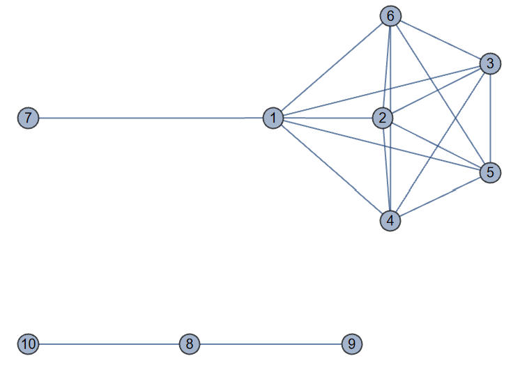
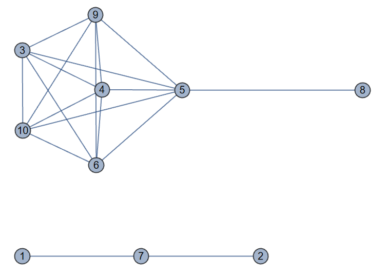
Figure 5: $\mathbf{g}^{1}$ (left) and $\mathbf{g}^{2}$ (right)

Suppose that the ex-ante distribution $p$ satisfies:

$$p(\mathbf{g})=\left\{\begin{array}[]{lr}\pi&\text{if }\mathbf{g}=\mathbf{g}^{1}\\ 1-\pi&\text{if }\mathbf{g}=\mathbf{g}^{2}\\ 0&\text{otherwise}\end{array}\right.$$

Let $N_{i}(\mathbf{g}^{k})$ denote the neighborhood set of the $i^{th}$ agent in the network $\mathbf{g}^{k}$, and observe that $N_{i}(\mathbf{g}^{1})\neq N_{i}(\mathbf{g}^{2})$, $\forall i\in N$. Consequently, belief consistency (Remark 1) implies that when either network $\mathbf{g}^{1}$ or $\mathbf{g}^{2}$ is realized, on learning their types agents will be able to determine the architecture of the entire network drawn. Moreover, since $p\in\Delta_{A}(G)$ is common knowledge, they also learn that all other players know the entire network architecture. As a result, equilibrium actions in this game of incomplete information will be identical to equilibrium actions under complete information. Setting $\lambda=0.11$, and concentrating on the equilibrium actions of agent 7 in each of the two networks, we find that $a_{7}^{*}(\mathbf{g}_{7}^{1})=1.26156$ and $a_{7}^{*}(\mathbf{g}_{7}^{2})=1.25026$. Therefore, even though $|N_{7}(\mathbf{g}^{2})|>|N_{7}(\mathbf{g}^{1})|$ and $N_{7}(\mathbf{g}^{2})\supset N_{7}(\mathbf{g}^{1})$, we have that $a_{7}^{*}(\mathbf{g}_{7}^{2})<a_{7}^{*}(\mathbf{g}_{7}^{1})$.

While action monotonicity in degrees is not a general property of this game, it may, nonetheless, arise in equilibrium when the ex-ante distribution is uniform over the set of all networks. Below we have the following characterization.

Proposition 2.

Let the underlying probability distribution be uniform over all networks. Then, equilibrium actions of agents over any realized network are given by:

$$a^{*}=1+\frac{\lambda d}{1-\frac{n\lambda}{2}},\quad\forall d\in\{0,1,2,\ldots,(n-1)\}$$

where $d$ is the degree of an agent in the realized network.

This proposition is similar to Proposition 2 in Galleotti et al. (2010), as well as Lemma 3 in Jackson (2019). Similar to our environment, they both study games under network uncertainty where agent information is restricted to first order connectivity. They provide Bayesian Nash equilibria where the actions of agents are monotonically increasing in their degree. Unlike our setup, however, ex-ante beliefs in their models are over degree distributions with types being represented by degrees themselves. Since degree distributions carry no vertex specific information other than degree, the key assumption driving their characterizations is anonymity. This property states that even though agents are aware of the number of agents they are connected to, they are unaware of the identity of these adjacent agents.

While our result provides the same quantitative insight as their findings, establishing a condition for monotonicity to arise in equilibrium, we do not require the anonymity assumption. As seen from Theorem 2, the BNE of this game is the result of an expected walk calculation. These walks are computed for all possible sequences of nodes originating from the agent who computes them and require agent identity to be accounted for. Clearly, these expected walks will be different for different ex-ante distributions that will place higher probability mass on specific sets of networks containing specific sets of walks. While anonymity is not imposed in our model, Proposition 2 provides a condition under which it appears to arise in equilibrium. This is due to the fact that equilibrium actions are completely characterized by agent degrees, which in turn only require first order connectivity information. However, this is a consequence of the uniform distribution assumption and the corresponding expected walks it induces. As the following lemma shows, the uniform case exhibits the special property that the expectation an agent has about every other agent’s degree (who is either connected or not connected to the former) is index invariant.

Lemma 2.

For any player $i$ denote by $\mathbb{E}_{i}(d_{j_{1}}),\mathbb{E}_{i}(d_{j_{2}}),..$ the agent’s interim expectations of any of its neighbor’s degree, any of its possible neighbor’s neighbor’s degree and so on. When the underlying probability distribution is uniform, we have:

$$\mathbb{E}_{i}\left[d_{j_{1}}\right]=\mathbb{E}_{i}\left[d_{j_{2}}\right]=\ldots\ldots=\frac{n}{2}$$

Consequently,

$$\beta_{i,t_{i}}^{(s)}=\left(\frac{n}{2}\right)^{s}$$

Uniformity in ex-ante beliefs provides the least amount of information with respect to identifying which walks are present in the network, inducing the trivial belief that all other agents have a degree equal to $\frac{n}{2}$. Consequently, each agent expects the complementarity strength of its action with any other agent due to a walk of length $s$ to be equal to $\lambda^{s}\left(\frac{n}{2}\right)^{s}$. This in turn generates equilibrium actions as in Proposition 1 and in-equilibrium anonymity.

Lastly, we note that Lemma 2 also speaks to a second assumption that drives Proposition 2 in Galleotti et al. (2010), namely degree independence. In their setup, independence of degrees implies that the belief of a player who has degree $d$, and that of another who has degree $d+1$, regarding the degrees of each of their neighbors are the same. In our case, the same property holds, but it arises endogenously as a result of ex-ante uniformity.

To sum up, through the uniform distribution this section provides us a precise way to see the connection between Galeotti et al. (2010) type degree models and walk based models. Regardless of the distribution, the degree model only counts the number of links an agent has; connectivity in the rest of the network does not matter and therefore it automatically invokes anonymity. Walk based models on the other hand rely on local information, i.e., agents know the identities of their direct connections. Nature draws a graph using different probability distributions and connectivity in the rest of the network matters. It turns out, however, that under the uniform distribution, agents expectations over every other agent’s degree are identical. Consequently, degrees determine everything and identity no longer matters. Anonymity, therefore, arises in-equilibrium under the uniform distribution. This may however not be the case for other admissible probability distributions.

5 Random Generation

In the previous sections, we have assumed that the ex-ante priors are prescribed by a probability measure over the set of all possible graphs. These ex-ante beliefs, however, are not unique in their ability to describe uncertainty over network topology. An alternative description, and one that has been widely employed in both theoretical (e.g. Dasaratha (2020)) and applied work (e.g. Zheng, Salganik, and Gelman (2006)), is random network generation. Formally, a random network model is a random matrix $\mathbf{g}$ whose entries $g_{ij}$ are distributed according to admissible densities $f_{i\sim j}$ such that the realizations of $\mathbf{g}$ are within some network class of interest. Intuitively, instead of having beliefs over specific network topologies $\mathbf{g}$, agents may have beliefs over the process itself that generates $\mathbf{g}$. In this section we argue that our approach to network games with incomplete information is robust to such ex-ante beliefs, and compute the corresponding Bayesian-Nash equilibria associated with a general class of generation models.

Generation Process

Our focus is on unweighted and undirected networks, and so we define the generation process via a collection of Bernoulli random variables. Consider the random variable $g_{i\sim j}$ which takes the value $1$ if there exists a link between $i$ and $j$, i.e., $i\sim j$, and $0$ otherwise. Since we do not consider self-loops, we set $g_{i\sim i}=0,\text{ for all }i\in N$. Its distribution is given by:

$$f_{i\sim j}(g_{ij})=\mathbb{P}\left(g_{i\sim j}=g_{ij}\right)=\begin{cases}\pi_{ij}&\text{ if }g_{ij}=1\\ 1-\pi_{ij}&\text{ if }g_{ij}=0\end{cases}$$

Recall that an undirected graph $\mathbf{g}$ is the collection of pairwise links between the players, or $\mathbf{g}:=\left\{i\sim j\right\}$ such that $i\sim j\in\mathbf{g}$ iff $j\sim i\in\mathbf{g}$. Thus, the probability of a graph $\mathbf{g}$ being realized is the joint probability of the existence of all the links in $\mathbf{g}$ and the non-existence of all the links that are not in $\mathbf{g}$. This is given by the joint distribution of $\left\{g_{i\sim j}:i<j\right\}$ which we represent by $f(.):\mathcal{G}_{n}\longrightarrow\left[0,1\right]$ where:

$$f(\mathbf{g})=\mathbb{P}\left(\left\{g_{i\sim j}=g_{ij}\in\left\{0,1\right\}:i<j\right\}\right)$$

Observe that if agents’ type sets $G_{i}$ and corresponding type space $G$ are the same as in section 2, then the Harsanyi transformation of the linear quadratic game remains the same as in this section as long as agents have common knowledge of $f(\mathbf{g})$. Moreover, the preceding network generation process guarantees that Nature will produce some unweighted and undirected network with certainty, implying that consistency in beliefs (Remark 1) is also preserved. Hence, agent beliefs over generation processes themselves induce similar type contingent beliefs as those over network topologies, preserving the functional form of the system of best responses that characterize the BNE. Consequently, Theorem 2 still holds with the expected complementarity strength arising from walks of different lengths being determined by agents’ updated beliefs over $f(\mathbf{g})$.

Erdos-Renyi and Homophilic Linkage

In order to gain some insight into how beliefs over network generation processes translate to equilibrium play, we impose the assumption that links are formed independently. In this case, ex-ante priors assume the following form:

$$f(\mathbf{g})=\prod_{i<j}f_{i\sim j}(g_{ij})=\prod_{i<j}\pi_{ij}^{g_{ij}}(1-\pi_{ij})^{1-g_{ij}}$$

Given link independence, it follows that a player $i$ who is of type $\mathbf{g}_{i}\in G_{i}$ will assign a probability to its neighbor being of type $\mathbf{g}_{j}\in G_{j}$ according to:

$$p(\mathbf{g}_{j}|\mathbf{g}_{i})=\prod_{k\neq i}\pi_{jk}^{g_{jk}}(1-\pi_{jk})^{1-g_{jk}}$$ (7)

Plugging equation (7) into the walk characterization of Theorem 2 gives the BNE of the game when agents have beliefs over a network generation process whose links are formed independently. In what follows we use these independent generation beliefs to characterize the Bayesian-Nash equilibria under a general class of generation models known as stochastic block models.

Definition 5.

Consider a partition of the agent set into $m\geq 1$ groups $A_{1},\,A_{2},..,\,A_{m}\subset N$ each consisting of $n_{i}$ agents respectively such that $\sum_{k}n_{k}=n$, $A_{i}\cap A_{j}=\emptyset,\,\forall i\neq j$ and $\cup_{k}A_{k}=N$. The network generation process follows a stochastic block model if

$$\pi_{ij}=\begin{cases}p_{k}&\text{if}\,i,j\in A_{k}\\ \epsilon&\text{otherwise}\end{cases}$$ (8)

where $p_{k},\epsilon\in[0,1]$ and $p_{k}\geq\epsilon$ for all $k\in\left\{1,2,\ldots,m\right\}$.

Observe that in the trivial case $m=1$, the stochastic block model reduces to the Erdos-Renyi random network model where all links are formed with equal probability $p$. When $m>1$ stochastic block generation allows for community structure and homophily to appear in the network.. The following proposition characterizes the BNE of the game for an arbitrary number of groups.

Proposition 3.

Suppose that the underlying network generation process follows a stochastic block model. Then, equilibrium actions of agents are given by:

$$a_{k}(\boldsymbol{d})=1+\lambda\sum_{l=1}^{m}\gamma_{kl}d_{l}$$

where $a_{k}(\boldsymbol{d})$ is the action of an agent who belongs in group $A_{k}$, and $\boldsymbol{d}\equiv\left(d_{1},d_{2},\ldots,d_{m}\right)$ is a vector of degrees in which $d_{l}$ denotes the agent’s degree with those agents group $l$, i.e. $d_{l}=\sum_{j\in A_{l}}g_{ij}$ where $i\in A_{k}$. The values of $\gamma_{kl}$ are given by the fixed point of the following system:

$$\gamma_{kl} =1+\lambda\gamma_{lk}[(n_{k}-1)\epsilon+1]+\lambda\gamma_{ll}\left(n_{l}-1\right)p_{l}+\lambda\sum_{\begin{subarray}{c}s=1\\ s\neq k,l\end{subarray}}^{m}\gamma_{ls}n_{s}\,\,\,\forall k\in\{1,..,\,m\},\,\forall\,l\neq k$$

$$\gamma_{kk} =1+\lambda\gamma_{kk}[(n_{k}-2)p_{k}+1]+\lambda\sum_{\begin{subarray}{c}s=1\\ s\neq k\end{subarray}}^{m}\gamma_{ks}n_{s}\epsilon\,\,\,\,\forall k\in\{1,..,\,m\}$$

First, let us consider the single group case where underlying network generation process follows an Erdos-Renyi model with linking probability $p$. In this case, equilibrium actions of agents reduce to:

$$a^{*}=1+\frac{\lambda d}{1-\lambda[(n-2)p+1]}\quad\forall d\in\left\{0,1,2,\ldots,(n-1)\right\}$$

where $d$ is the degree of an agent in the realized network. This closed form characterization resembles the one in Proposition 2 where ex-ante beliefs are uniform over the set of all networks. If the linking probability satisfies $p=\frac{1}{2}$, then the two characterizations are identical. Similar to the intuition behind Proposition 2, when all links are formed with equal probability $p$ every agent has the trivial belief that all others have a degree of $(n-2)p+1$. Therefore, each agent expects the complementarity strength of its action with any other agent due to a walk of length $s$ to be equal to $\lambda^{s}\left((n-2)p+1\right)^{s}$. As in the uniform case, these Erdos-Renyi beliefs produce in-equilibrium anonymity.

Next consider $m>1$. In this case, unlike Proposition 2 and Erdos-Renyi generation, the equilibrium exhibits a group identity property. In particular, while the degree of an agent is important in determining the total complementarity it expects to extract from the network, agents extract different complementarity strengths depending on the identity of the group in which their neighbors belong to. Specifically, an agent in group $A_{k}$ extracts complementarities from its intra ($d_{k}$) and inter-group ($d_{l}$) neighbors according to the maginitutes of parameters $\gamma_{kk}$ and $\gamma_{kl}$. Each of these parameters represents the extent to which walks that are formed via group-specific neighbors are complementary.

The intuition behind this complementarity decomposition is best understood when $m=2$. In this case, the linear system in Proposition 3 reduces to:

$$\gamma_{11} =1+\lambda\gamma_{11}[(n_{1}-2)p_{1}+1]+\lambda\gamma_{12}n_{2}\epsilon$$

$$\gamma_{12} =1+\lambda\gamma_{21}[(n_{1}-1)\epsilon+1]+\lambda\gamma_{22}(n_{2}-1)p_{2}$$

$$\gamma_{21} =1+\lambda\gamma_{11}(n_{1}-1)p_{1}+\lambda\gamma_{12}[(n_{2}-1)\epsilon+1]$$

$$\gamma_{22} =1+\lambda\gamma_{21}n_{1}\epsilon+\lambda\gamma_{22}[(n_{2}-2)p_{2}+1]$$

When the population consists of two groups, stochastic block generation gives rise to the interim belief that an agent in any given group can form four different types of walks. Fixing an agent $i\in A_{1}$, these walks assume the following forms: (i) $i\sim j\sim..\sim k$ s.t $j,k\in A_{1}$, (ii) $i\sim j\sim..\sim k$ s.t $j\in A_{1}$, $k\in A_{2}$, (iii) $i\sim j\sim..\sim k$ s.t $j\in A_{2}$, $k\in A_{1}$, and (iv) $i\sim j\sim..\sim k$ s.t $j,k\in A_{2}$. Since links are formed independently, and since all links of a particular type are formed with the same probability, this implies that any two walks of the same type provide the same complementarity strength.

To see how these strengths are determined, consider an agent $i\in A_{1}$. The agent knows that within its group, all links have a probability $p_{1}$ being realized. Since links are independent, this implies that the agent expects that all others within its own group have a degree of $(n_{1}-2)p+1$. Hence, if $\gamma_{11}$ represents the spillover strength extracted from each walk of type (i), then their total strength is $\lambda\gamma_{11}[(n_{1}-2)p_{1}+1]$. Next, the agent also knows that its neighbors within the group are connected to others across the group with probability $\epsilon$. Therefore, it also expects to have walks via its intra group neighbors to those agents in $A_{2}$. Since the agent expects that its intra group neighbors have $n_{2}\epsilon$ inter group neighbors, if $\gamma_{12}$ represents the spillover strength extracted from each walk of type (ii), then their total strength is $\lambda\gamma_{12}n_{2}\epsilon$. Summing the two terms, and multiplying by the agents intra group degree $d_{1}$ gives the total complementarity the agent expects to extract from walks that start within its own group to all other agents (i.e. type (i) and type (ii) walks).

Next, consider inter group spillovers. By link independence, an agent $i\in A_{1}$ expects any of its inter group neighbors have $(n_{1}-1)\epsilon+1$ inter groups neighbors and $(n_{2}-1)p_{2}$ intra group neighbors of their own. Therefore, a similar argument as above establishes that $\lambda\gamma_{21}[(n_{1}-1)\epsilon+1]$ and $\lambda\gamma_{22}(n_{2}-1)p_{2}$ are the total complementarity strength extracted from type (iii) and type (iv) walks respectively. Summing the two terms, and multiplying by the agents inter group degree $d_{2}$ gives the total complementarity the agent expects to extract from walks that start across its group to all other agents (i.e., type (iii) and type (iv) walks).

In the special case where the intra-group linking probabilities are the same, the magnitudes of these complementarity strengths are completely characterized by group size.

Lemma 3.

Suppose that $m=2$, $p_{1}=p_{2}$ and $n_{1},\,n_{2}\geq 3$. If $n_{1}\geq n_{2}+2$, then $\gamma_{11}>\gamma_{12}$ and vice-versa. However, if $n_{1}=n_{2}$ then $\gamma_{12}>\gamma_{11}$.

6 Conclusion

We study a linear quadratic network game of incomplete information in which agents’ information is restricted only to the identity of their neighbors. We characterize Bayesian-Nash equilibria, demonstrating that agents make use of local information to form beliefs about the number of walks they have in the network, and consequently the complementarity strength of their action with all other agents. Unlike other models in the literature, we show that local information captured by identity and network position play a crucial role in allowing agents to determine this complementarity. Even though equilibria for certain ex-ante prior beliefs exhibit in-equilibrium anonymity, this anonymity is a consequence of trivial information structures such as uniform priors or an Erdos-Renyi network generation process.

The proposed model is flexible enough that allows for the formal study of strategic behavior in networks under any form of ex-ante beliefs, regardless if these are over network topology or network generation. For any given prior, as long as agent information is restricted to their local neighborhood, the BNE of this game can be computed via the walk characterization developed above and can be directly compared to its complete information Nash equilibrium counterpart. In turn, this allows for the study of how rational agent behavior will deviate from complete information behavior within the multiplicity of network systems that have been modeled via the canonical linear quadratic game.

Appendix A: Proofs of Main Results

Proof of Theorem 1

Define a mapping $P:\mathbb{R}^{n\gamma}\longrightarrow\mathbb{R}^{n\gamma}$, such that

$$P(\mathbf{a})=\mathbf{1}+\lambda\mathbb{B}\mathbf{a}$$

with $\mathbb{B}$ as defined in section 3.1. Let $(\mathbb{R}^{n\gamma},\left\|.\right\|_{\infty})$ be a metric space with $\left\|.\right\|_{\infty}$ being the sup-norm on $\mathbb{R}^{n\gamma}$. Hence, we can write:

$$\left\|P(\mathbf{x})-P(\mathbf{y})\right\|_{\infty} =\left|\lambda\right|\left\|\mathbb{B}(x-y)\right\|_{\infty}$$

$$\leq\lambda(n-1)\left\|x-y\right\|_{\infty}$$

$$=r\left\|x-y\right\|_{\infty}$$

where the first inequality results from the fact that $\left\|\mathbb{B}\mathbf{a}\right\|_{\infty}\leq(n-1)\left\|\mathbf{a}\right\|_{\infty}$ since the rows of $\mathbb{B}$ sum to $n-1$. Thus, we get

$$\left\|P(\mathbf{x})-P(\mathbf{y})\right\|_{\infty}\leq r\left\|x-y\right\|_{\infty}$$

so that $P$ is a contraction mapping on $\mathbb{R}^{n\gamma}$ as long as $r\in[0,1)$. This holds if:

$$0\leq\lambda(n-1)\leq 1\Rightarrow 0\leq\lambda<\frac{1}{n-1}$$

Hence, for $0\leq\lambda<\frac{1}{n-1}$, $P$ is a contraction mapping on $\mathbb{R}^{n\gamma}$ and $(\mathbb{R}^{n\gamma},\left\|.\right\|_{\infty})$ is a complete metric space. Therefore, by the Banach fixed point theorem, there exists an unique $\mathbf{a}^{*}\in\mathbb{R}^{n\gamma}$, such that

$$P(\mathbf{a}^{*})=\mathbf{a}^{*}\Rightarrow\mathbf{a}^{*}=\mathbf{1}+\lambda\mathbb{B}\mathbf{a}^{*}$$

Consequently, there exists an unique pure strategy BNE for the game $\mathbf{\boldsymbol{\Gamma}}$ whenever $\lambda\in\left[0,\frac{1}{n-1}\right)$.

$\blacksquare$

Proof of Theorem 2

The best responses for all players can be written in vector notation as

$$\mathbf{a}=\mathbf{1}+\lambda\mathbb{B}\mathbf{a}$$

Then the equilibrium actions for $\lambda\in\left[0,\frac{1}{n-1}\right)$ can be written in the form

$$\mathbf{a}^{*} =\left(\mathbf{I}-\lambda\mathbb{B}\right)^{-1}\cdot\mathbf{1}$$

$$=\mathbf{1}+\lambda\mathbb{B}\cdot\mathbf{1}+\lambda^{2}\mathbb{B}^{2}\cdot\mathbf{1}+\ldots\ldots$$

For an agent $i\in N$ of type $\mathbf{g}_{i}^{t_{i}}$ the equilibrium action is given by

$$a_{i}^{*}\left(\mathbf{g}_{i}^{t_{i}}\right)=1+\lambda\left[\mathbb{B}\cdot\mathbf{1}\right]_{i,t_{i}}+\lambda^{2}\left[\mathbb{B}^{2}\cdot\mathbf{1}\right]_{i,t_{i}}+\ldots\ldots$$

Then

$$\beta_{i,t_{i}}^{(1)} =\left[\mathbb{B}\cdot\mathbf{1}\right]_{i,t_{i}} \beta_{i,t_{i}}^{(2)} =\left[\mathbb{B}^{2}\cdot\mathbf{1}\right]_{i,t_{i}}$$

$$=\sum_{j=1}^{n}\sum_{t_{j}=1}^{\gamma}\left[G_{i\sim j}\right]_{t_{i},t_{j}} =\left[\mathbb{B}\cdot\left(\mathbb{B}\cdot\mathbf{1}\right)\right]_{i,t_{i}}$$

$$=\sum_{j=1}^{n}\sum_{t_{j}=1}^{\gamma}g_{ij}^{t_{i}}p(\mathbf{g}_{j}^{t_{j}}|\mathbf{g}_{i}^{t_{i}}) =\sum_{j=1}^{n}\sum_{t_{j}=1}^{\gamma}\left[G_{i\sim j}\right]_{t_{i},t_{j}}\beta_{j,t_{j}}^{(1)}$$

$$=\sum_{j=1}^{n}g_{ij}^{t_{i}}\sum_{t_{j}=1}^{\gamma}p(\mathbf{g}_{j}^{t_{j}}|\mathbf{g}_{i}^{t_{i}}) =\sum_{j=1}^{n}\sum_{t_{j}=1}^{\gamma}g_{ij}^{t_{i}}p(\mathbf{g}_{j}^{t_{j}}|\mathbf{g}_{i}^{t_{i}})\sum_{k=1}^{n}g_{jk}^{t_{j}}$$

$$=\sum_{j=1}^{n}g_{ij}^{t_{i}} =\sum_{j=1}^{n}\sum_{k=1}^{n}\sum_{t_{j}=1}^{\gamma}g_{ij}^{t_{i}}g_{jk}^{t_{j}}p(\mathbf{g}_{j}^{t_{j}}|\mathbf{g}_{i}^{t_{i}})$$

This calculation generalizes for $\beta_{i,t_{i}}^{(s)}$.

$\blacksquare$

Proof of Proposition 1

Since the agents are endowed with the belief that the actual network over which the game is being played assumes a core-periphery architechture, any agent after realizing the identity of their neighbors can infer if they are in the core or in the periphery. Thus the type space for this case can be mapped to $\left\{P_{k}:k=0,1,2,....,n-2\right\}\cup\left\{C\right\}$, where $P_{k}$ is the type of an agent in the periphery with degree $k$, i.e. the size of the core for that realized network is $k$ and $C$ is the type of an agent who is in the core. Let $t_{i}$ denote the type of any agent $i$. If an agent $i$ realizes that they are in the periphery, i.e. $t_{i}=P_{k}$, they realize that their direct connections are only the players in the core and hence the best response for them is given by

$$a(P_{k})=1+\lambda ka(C)$$ (9)

where $a(C)$ is the action taken by a player in the core. The best response for a Core agent $i$ who is connected to everyone is given by

$$\begin{aligned} a(C)=&1+\lambda\end{aligned}\sum_{j=1}^{n}g_{ij}\left(\sum_{k=1}^{n-2}p\left(t_{j}=P_{k}\mid t_{i}=C\right)a\left(P_{k}\right)+p\left(t_{j}=C\mid t_{i}=C\right)a(C)\right)$$ (10)

Again using Baye’s rule we can compute

$$p\left(t_{j}=P_{k}\mid t_{i}=C\right)=\frac{p\left(t_{j}=P_{k},t_{i}=C\right)}{p\left(t_{i}=C\right)} =\frac{\binom{n-2}{k-1}}{\sum_{k=1}^{n}\binom{n-1}{k-1}-\binom{n-1}{n-2}}$$

$$p\left(t_{j}=C\mid t_{i}=C\right)=\frac{p\left(t_{j}=C,t_{i}=C\right)}{p\left(t_{i}=C\right)} =\frac{\sum_{k=2}^{n}\binom{n-2}{k-2}-\binom{n-2}{n-3}}{\sum_{k=1}^{n}\binom{n-1}{k-1}-\binom{n-1}{n-2}}$$

where $p\left(t_{j}=P_{k},t_{i}=C\right)=\frac{\binom{n-2}{k-1}}{|\mathcal{G}_{n}^{CP}|}$ and $p\left(t_{i}=C\right)=\frac{\sum_{k=1}^{n}\binom{n-1}{k-1}-\binom{n-1}{n-2}}{|\mathcal{G}_{n}^{CP}|}$, as the underlying distribution is uniform defined over all core-periphery networks on $n$-nodes. Similar calculations follow for $p\left(t_{j}=C,t_{i}=C\right)$.

Then putting the values in (10) the best responses of a Core agent can be written as:

$$a(C)=1+\frac{(n-1)\lambda}{\Delta}\left[\sum_{k=1}^{n-2}\binom{n-2}{k-1}a(P_{k})+\left\{\sum_{k=2}^{n}\binom{n-2}{k-2}-\binom{n-2}{n-3}\right\}a(C)\right]$$ (11)

where $\Delta=\sum_{k=1}^{n}\binom{n-1}{k-1}-\binom{n-1}{n-2}$.

Using (9) the best response of a core player can be re-written as:

$$a(C)=1+\frac{(n-1)\lambda}{\Delta}\left[\sum_{k=1}^{n-2}\binom{n-2}{k-1}+\lambda a(C)\sum_{k=1}^{n-2}k\binom{n-2}{k-1}+\left\{\sum_{k=2}^{n}\binom{n-2}{k-2}-\binom{n-2}{n-3}\right\}a(C)\right]$$

The action exerted by a Core player is then given by

$$a(C)=\frac{1+\lambda X}{1-\lambda Z-\lambda^{2}Y}$$ (12)

where

$$X=(n-1)\frac{\sum_{k=1}^{n-2}\binom{n-2}{k-1}}{\Delta},\quad Y=(n-1)\frac{\sum_{k=1}^{n-2}k\binom{n-2}{k-1}}{\Delta},\quad Z=(n-1)\frac{\sum_{k=2}^{n}\binom{n-2}{k-2}-\binom{n-2}{n-3}}{\Delta}$$

Looking into the terms $X,Y,Z$ we see that:

• Consider the following random variable $X_{j}$ for an agent $i$ who is in the Core (i.e. $i\in C$), where

  $$X_{j}=\begin{cases}1\quad&\text{if }j\in C\text{ for }g_{ij}=1\\ 0\quad&\text{if }j\notin C\text{ for }g_{ij}=1\end{cases}$$

  and

  $$P(X_{j}=1)=\frac{\sum_{k=2}^{n}\binom{n-2}{k-2}-\binom{n-2}{n-3}}{\Delta}$$

  Then for the agent $i$ the expected size of the core conditional on the fact that they are in the core, is given by

  $$\mathbb{E}\left[n_{co}|i\in C\right]=\mathbb{E}_{i}\left[n_{co}\right]=\sum_{j=1}^{n}g_{ij}P(X_{j}=1)+1=Z+1$$

  Hence, $\mathbb{E}_{i}\left[n_{co}-1\right]=Z$.

• Consider the following random variable $Y_{j}$ for an agent $i$ who is in the Core (i.e. $i\in C$), where

  $$Y_{j}=\begin{cases}1\quad&\text{if }j\in P\text{ for }g_{ij}=1\\ 0\quad&\text{if }j\notin P\text{ for }g_{ij}=1\end{cases}$$

  and

  $$P(Y_{j}=1)=\frac{\sum_{k=1}^{n-1}\binom{n-2}{k-1}-\binom{n-2}{n-2}}{\Delta}$$

  Then for the agent $i$ the expected number of agents in the periphery conditional on the fact that they are in the core, is given by

  $$\mathbb{E}\left[n_{p}|i\in C\right]=\mathbb{E}_{i}\left[n_{p}\right]=\sum_{j=1}^{n}g_{ij}P(Y_{j}=1)=X$$

  Hence, $\mathbb{E}_{i}\left[n_{p}\right]=X$.

• For any agent $i\in C$ let $d_{p}$ be the random variable denoting the degree of their neighbor $j$ if they are in the periphery. Then the expected degree of agent $i$’s neighbor if they are in the periphery, conditional on the fact that $i\in C$ is given by:

  $$\mathbb{E}\left[d_{p}|i\in C\right]=\frac{\sum_{k=1}^{n-2}k\binom{n-2}{k-1}}{\Delta}$$

  Thus for the agent $i$, the complementary strength that they can extract from the peripheral nodes through the walks of length 2 is

  $$\mathbb{E}\left[n_{p}n_{co}|i\in C\right]=\mathbb{E}_{i}\left[n_{p}n_{co}\right]=(n-1)\mathbb{E}\left[d_{p}|i\in C\right]=Y$$

Thus the equilibrium action taken by an agent in the core under incomplete information of the graph structure can be written as:

$$a_{co_{i}}^{*}=a\left(C\right)=\frac{1+\lambda\mathbb{E}_{i}\left[n_{p}\right]}{1-\lambda\mathbb{E}_{i}\left[n_{co}-1\right]-\lambda^{2}\mathbb{E}_{i}\left[n_{p}n_{co}\right]}$$

$\blacksquare$

Proof of Proposition 2

Consider an agent $i$ of type $\mathbf{g}_{i}^{t_{i}}$ such that $\sum_{j\in N}g_{ij}^{t_{i}}=d_{i}$. For any $j\in\text{N}\left(\mathbf{g}_{i}^{t_{i}}\right)$, the updated belief of $i$ about $j$’s type is given by

$$p\left(\mathbf{g}_{j}^{t_{j}}\mid\mathbf{g}_{i}^{t_{i}}\right)=\frac{p\left(\mathbf{g}_{j}^{t_{j}},\mathbf{g}_{i}^{t_{i}}\right)}{p\left(\mathbf{g}_{i}^{t_{i}}\right)}=\frac{2^{(n-3)(n-2)/2}}{2^{(n-1)(n-2)/2}}=\frac{1}{2^{n-2}}$$

where $p\left(\mathbf{g}_{j}^{t_{j}},\mathbf{g}_{i}^{t_{i}}\right)=\frac{2^{(n-3)(n-2)/2}}{|\mathcal{G}_{n}|}$ and $p\left(\mathbf{g}_{i}^{t_{i}}\right)=\frac{2^{(n-1)(n-2)/2}}{|\mathcal{G}_{n}|}$, as the underlying probability distribution is uniform. We see that the updated beliefs are independent of the identity of the agent as well as their neighbor. This is also independent of the types of each player. Thus, uniformity in ex-ante belifes implies that the best response of any agent $i$ whose type is such that it is connected to $d$ agents, is identical to that of another agent $j$ who is also connected to $d$ agents. We may, therefore, characterise best responses with respect to degrees and hence for any agent $i$ of degree $d$ the best response reduces to

$$a(d)=1+\lambda d\sum_{d=1}^{n-1}\frac{{n-2\choose d-1}}{2^{n-2}}a(d)$$ (13)

Multiplying both sides of (13) by ${n-2\choose d-1}$, we get

$$\therefore{n-2\choose d-1}a(d) ={n-2\choose d-1}+\left[\frac{\lambda}{2^{n-2}}\sum_{d=1}^{n-1}{n-2\choose d-1}a(d)\right]{n-2\choose d-1}d$$

$$\Rightarrow\sum_{d=1}^{n-1}{n-2\choose d-1}a(d) =\sum_{d=1}^{n-1}{n-2\choose d-1}+\left[\frac{\lambda}{2^{n-2}}\sum_{d=1}^{n-1}{n-2\choose d-1}a(d)\right]\sum_{d=1}^{n-1}{n-2\choose d-1}d$$

$$\Rightarrow\sum_{d=1}^{n-1}{n-2\choose d-1}a(d) =2^{n-2}+\left[\frac{\lambda}{2^{n-2}}\sum_{d=1}^{n-1}{n-2\choose d-1}a(d)\right]\sum_{d=1}^{n-1}{n-2\choose d-1}d$$

Again, we know that

$$\sum_{d=1}^{n-1}{n-2\choose d-1}d =\sum_{d=1}^{n-1}(d-1){n-2\choose d-1}+\sum_{d=1}^{n-1}{n-2\choose d-1}$$

$$=\sum_{d=1}^{n-1}\frac{(n-2)!}{(d-2)!(n-2-\overline{d-1})!}+2^{n-2}$$

$$=(n-2)\sum_{d=2}^{n-1}{n-3\choose d-2}+2^{n-2}$$

$$=(n-2)2^{n-3}+2^{n-2}$$

Putting the value of $\sum_{d=1}^{n-1}{n-2\choose d-1}d$ we get

$$\sum_{d=1}^{n-1}{n-2\choose d-1}a(d) =2^{n-2}+\left[\frac{\lambda}{2^{n-2}}\sum_{d=1}^{n-1}{n-2\choose d-1}a(d)\right]\left((n-2)2^{n-3}+2^{n-2}\right)$$

$$=\frac{2^{n-2}}{1-\frac{n\lambda}{2}}$$

Thus putting this value back in the best response equation (13) we get the equilibrium actions

$$a(d)=1+\frac{\lambda d}{1-\frac{n\lambda}{2}},\quad\forall d\in\{0,1,2,\ldots,(n-1)\}$$ (14)

$\blacksquare$

Proof of Proposition 3

Consider an agent $i$ of type $\mathbf{g}_{i}$ in group $A_{k}$, with a degree vector $\boldsymbol{d}_{i}\equiv\left(d_{1}^{i},d_{2}^{i},\ldots,d_{m}^{i}\right)$, where $d_{l}^{i}$ corresponds to the agent $i$’s degree in group $l$, i.e. $d_{l}^{i}=\sum_{j\in A_{l}}g_{ij}$. If their neighbor $j$ of type $\mathbf{g}_{j}$ in group $A_{l}$, has a degree vector $\boldsymbol{d}\equiv\left(d_{1},d_{2},\ldots,d_{m}\right)$ then from (7) the updated belief of agent $i$ takes the form,

$$p(\mathbf{g}_{j}|\mathbf{g}_{i})=\begin{cases}p_{l}^{d_{l}}(1-p_{l})^{n_{l}-d_{l}-1}\epsilon^{d_{k}-1}(1-\epsilon)^{n_{k}-d_{k}}\prod_{\begin{subarray}{c}q=1\\ q\neq k,l\end{subarray}}^{m}\epsilon^{d_{q}}(1-\epsilon)^{n_{q}-d_{q}}&\text{if }k\neq l\\ p_{k}^{d_{k}-1}(1-p_{k})^{n_{k}-d_{k}-1}\prod_{\begin{subarray}{c}q=1\\ q\neq k\end{subarray}}^{m}\epsilon^{d_{k}}(1-\epsilon)^{n_{k}-d_{k}}&\text{if }k=l\end{cases}$$

Thus for the agent $i$ the updated belief about his neighbor’s type is independent of the identity of their neighbors and is dependent only on their degrees. As a result, the type space for this special case can be mapped to the degree space. We can write the best response of the agent $i\in A_{k}$ of degree vector $\boldsymbol{d}_{i}\equiv\left(d_{1}^{i},d_{2}^{i},\ldots,d_{m}^{i}\right)$ with respect to their degrees,

$$a_{k}(\boldsymbol{d}_{i})=1+\lambda\sum_{l=1}^{m}\gamma_{kl}d_{l}^{i}$$ (15)

where, for $k\neq l$:

$$\gamma_{kl}=\sum_{d_{l}=0}^{n_{l}-1}\binom{n_{l}-1}{d_{l}}p_{l}^{d_{l}}(1-p_{l})^{n_{l}-d_{l}-1}\sum_{d_{k}=1}^{n_{k}}\binom{n_{k}-1}{d_{k}-1}\epsilon^{d_{k}-1}(1-\epsilon)^{n_{k}-d_{k}}\prod_{\begin{subarray}{c}q=1\\ q\neq k,l\end{subarray}}^{m}\sum_{d_{q}=0}^{n_{q}}\binom{n_{q}}{d_{q}}\epsilon^{d_{q}}(1-\epsilon)^{n_{q}-d_{q}}a_{l}\left(\boldsymbol{d}\right)$$

and if $k=l$

$$\gamma_{kk}=\sum_{d_{k}=1}^{n_{k}-1}\binom{n_{k}-2}{d_{k}-1}p_{k}^{d_{k}-1}(1-p_{k})^{n_{k}-d_{k}-1}\prod_{\begin{subarray}{c}q=1\\ q\neq k\end{subarray}}^{m}\sum_{d_{q}=0}^{n_{q}}\binom{n_{q}-1}{d_{q}-1}\epsilon^{d_{q}}(1-\epsilon)^{n_{q}-d_{q}}a_{k}(\boldsymbol{d})$$

Then from equation (15) we can write, when $k\neq l$

$$\gamma_{kl} =\sum_{d_{l}=0}^{n_{l}-1}\binom{n_{l}-1}{d_{l}}p_{l}^{d_{l}}(1-p_{l})^{n_{l}-d_{l}-1}\sum_{d_{k}=1}^{n_{k}}\binom{n_{k}-1}{d_{k}-1}\epsilon^{d_{k}-1}(1-\epsilon)^{n_{k}-d_{k}}\prod_{\begin{subarray}{c}q=1\\ q\neq k,l\end{subarray}}^{m}\sum_{d_{q}=0}^{n_{q}}\binom{n_{q}}{d_{q}}\epsilon^{d_{q}}(1-\epsilon)^{n_{q}-d_{q}}$$

$$+ \lambda\sum_{s=1}^{m}\gamma_{ls}d_{s}\sum_{d_{l}=0}^{n_{l}-1}\binom{n_{l}-1}{d_{l}}p_{l}^{d_{l}}(1-p_{l})^{n_{l}-d_{l}-1}\sum_{d_{k}=1}^{n_{k}}\binom{n_{k}-1}{d_{k}-1}\epsilon^{d_{k}-1}(1-\epsilon)^{n_{k}-d_{k}}\prod_{\begin{subarray}{c}q=1\\ q\neq k,l\end{subarray}}^{m}\sum_{d_{q}=0}^{n_{q}}\binom{n_{q}}{d_{q}}\epsilon^{d_{q}}(1-\epsilon)^{n_{q}-d_{q}}$$

$$=1+ \lambda\sum_{\begin{subarray}{c}s=1\\ s\neq l,k\end{subarray}}^{m}\gamma_{ls}\sum_{d_{l}=0}^{n_{l}-1}\binom{n_{l}-1}{d_{l}}p_{l}^{d_{l}}(1-p_{l})^{n_{l}-d_{l}-1}\sum_{d_{k}=1}^{n_{k}}\binom{n_{k}-1}{d_{k}-1}\epsilon^{d_{k}-1}(1-\epsilon)^{n_{k}-d_{k}}\prod_{\begin{subarray}{c}q=1\\ q\neq k,l\end{subarray}}^{m}\sum_{d_{q}=0}^{n_{q}}d_{s}\binom{n_{q}}{d_{q}}\epsilon^{d_{q}}(1-\epsilon)^{n_{q}-d_{q}}$$

$$+ \lambda\gamma_{lk}\sum_{d_{l}=0}^{n_{l}-1}\binom{n_{l}-1}{d_{l}}p_{l}^{d_{l}}(1-p_{l})^{n_{l}-d_{l}-1}\sum_{d_{k}=1}^{n_{k}}d_{k}\binom{n_{k}-1}{d_{k}-1}\epsilon^{d_{k}-1}(1-\epsilon)^{n_{k}-d_{k}}\prod_{\begin{subarray}{c}q=1\\ q\neq k,l\end{subarray}}^{m}\sum_{d_{q}=0}^{n_{q}}\binom{n_{q}}{d_{q}}\epsilon^{d_{q}}(1-\epsilon)^{n_{q}-d_{q}}$$

$$+ \gamma_{ll}\sum_{d_{l}=0}^{n_{l}-1}d_{l}\binom{n_{l}-1}{d_{l}}p_{l}^{d_{l}}(1-p_{l})^{n_{l}-d_{l}-1}\sum_{d_{k}=1}^{n_{k}}\binom{n_{k}-1}{d_{k}-1}\epsilon^{d_{k}-1}(1-\epsilon)^{n_{k}-d_{k}}\prod_{\begin{subarray}{c}q=1\\ q\neq k,l\end{subarray}}^{m}\sum_{d_{q}=0}^{n_{q}}\binom{n_{q}}{d_{q}}\epsilon^{d_{q}}(1-\epsilon)^{n_{q}-d_{q}}$$

Thus evaluating them we get that:

$$\prod_{\begin{subarray}{c}q=1\\ q\neq k,l\end{subarray}}^{m}\sum_{d_{q}=0}^{n_{q}}d_{s}\binom{n_{q}}{d_{q}}\epsilon^{d_{q}}(1-\epsilon)^{n_{q}-d_{q}} =\sum_{d_{s}=0}^{n_{s}}d_{s}\binom{n_{s}}{d_{s}}\epsilon^{d_{s}}(1-\epsilon)^{n_{s}-d_{s}}\prod_{\begin{subarray}{c}q=1\\ q\neq k,l,s\end{subarray}}^{m}\sum_{d_{q}=0}^{n_{q}}d_{s}\binom{n_{q}}{d_{q}}\epsilon^{d_{q}}(1-\epsilon)^{n_{q}-d_{q}}$$

$$=n_{s}\epsilon\sum_{d_{s}=1}^{n_{s}}\binom{n_{s}-1}{d_{s}-1}\epsilon^{d_{s}-1}(1-\epsilon)^{n-d_{s}}$$

$$=n_{s}\epsilon$$

where, the first equality is due to the fact that $\sum_{d_{q}=0}^{n_{q}}d_{s}\binom{n_{q}}{d_{q}}\epsilon^{d_{q}}(1-\epsilon)^{n_{q}-d_{q}}=1$, and the second equality is due to the fact that $\sum_{d_{s}=1}^{n_{s}}\binom{n_{s}-1}{d_{s}-1}\epsilon^{d_{s}-1}(1-\epsilon)^{n-d_{s}}=1$.

$$\sum_{d_{k}=1}^{n_{k}}d_{k}\binom{n_{k}-1}{d_{k}-1}\epsilon^{d_{k}-1}(1-\epsilon)^{n_{k}-d_{k}}$$

$$= (n_{k}-1)\epsilon\sum_{d_{k}=2}^{n_{k}}\binom{n_{k}-2}{d_{k}-2}\epsilon^{d_{k}-2}(1-\epsilon)^{n_{k}-d_{k}}+\sum_{d_{k}=1}^{n_{k}}\binom{n_{k}-1}{d_{k}-1}\epsilon^{d_{k}-1}(1-\epsilon)^{n_{k}-d_{k}}$$

$$= (n_{k}-1)\epsilon+1$$

And,

$$\sum_{d_{l}=0}^{n_{l}-1}d_{l}\binom{n_{l}-1}{d_{l}}p_{l}^{d_{l}}(1-p_{l})^{n_{l}-d_{l}-1} =(n_{l}-1)p_{l}\sum_{d_{l}=1}^{n_{l}-1}\binom{n_{l}-2}{d_{l}-1}p_{l}^{d_{l}-1}(1-p_{l})^{n_{l}-d_{l}-1}$$

$$=(n_{l}-1)p_{l}$$

Thus, we can write $\gamma_{kl}$ to be

$$\gamma_{kl}=1+\lambda\sum_{s\neq l,k}\gamma_{ls}n_{s}\epsilon+\lambda\gamma_{lk}\left[(n_{k}-1)\epsilon+1\right]+\lambda\gamma_{kk}\left(n_{l}-1\right)p_{l}$$ (16)

Next consider the case when $l=k$, we can write

$$\gamma_{kk} =\sum_{d_{k}=1}^{n_{k}-1}\binom{n_{k}-2}{d_{k}-1}p_{k}^{d_{k}-1}(1-p_{k})^{n_{k}-d_{k}-1}\prod_{\begin{subarray}{c}q=1\\ q\neq k\end{subarray}}^{m}\sum_{d_{q}=0}^{n_{q}}\binom{n_{q}-1}{d_{q}-1}\epsilon^{d_{q}}(1-\epsilon)^{n_{q}-d_{q}}$$

$$+\lambda\sum_{s=1}^{m}\gamma_{ks}d_{s}\sum_{d_{k}=1}^{n_{k}-1}\binom{n_{k}-2}{d_{k}-1}p_{k}^{d_{k}-1}(1-p_{k})^{n_{k}-d_{k}-1}\prod_{\begin{subarray}{c}q=1\\ q\neq k\end{subarray}}^{m}\sum_{d_{q}=0}^{n_{q}}\binom{n_{q}-1}{d_{q}-1}\epsilon^{d_{q}}(1-\epsilon)^{n_{q}-d_{q}}$$

$$=1+\lambda\sum_{\begin{subarray}{c}s=1\\ s\neq k\end{subarray}}^{m}\gamma_{ks}\sum_{d_{k}=1}^{n_{k}-1}\binom{n_{k}-2}{d_{k}-1}p_{k}^{d_{k}-1}(1-p_{k})^{n_{k}-d_{k}-1}\prod_{\begin{subarray}{c}q=1\\ q\neq k\end{subarray}}^{m}\sum_{d_{q}=0}^{n_{q}}d_{s}\binom{n_{q}-1}{d_{q}-1}\epsilon^{d_{q}}(1-\epsilon)^{n_{q}-d_{q}}$$

$$+\lambda\gamma_{kk}\sum_{d_{k}=1}^{n_{k}-1}d_{k}\binom{n_{k}-2}{d_{k}-1}p_{k}^{d_{k}-1}(1-p_{k})^{n_{k}-d_{k}-1}\prod_{\begin{subarray}{c}q=1\\ q\neq k\end{subarray}}^{m}\sum_{d_{q}=0}^{n_{q}}\binom{n_{q}-1}{d_{q}-1}\epsilon^{d_{q}}(1-\epsilon)^{n_{q}-d_{q}}$$

For the similar reasons as mentioned above, we have that

$$\prod_{\begin{subarray}{c}q=1\\ q\neq k\end{subarray}}^{m}\sum_{d_{q}=0}^{n_{q}}d_{s}\binom{n_{q}-1}{d_{q}-1}\epsilon^{d_{q}}(1-\epsilon)^{n_{q}-d_{q}}=n_{s}\epsilon$$

And evaluating the other part of the sum, we get

$$\sum_{d_{k}=1}^{n_{k}-1}d_{k}\binom{n_{k}-2}{d_{k}-1}p_{k}^{d_{k}-1}(1-p_{k})^{n_{k}-d_{k}-1}$$

$$= \left(n_{k}-2\right)p_{k}\sum_{d_{k}=2}^{n_{k}-1}\binom{n_{k}-3}{d_{k}-2}p_{k}^{d_{k}-2}(1-p_{k})^{n_{k}-d_{k}-1}+\sum_{d_{k}=1}^{n_{k}-1}\binom{n_{k}-2}{d_{k}-1}p_{k}^{d_{k}-1}(1-p_{k})^{n_{k}-d_{k}-1}$$

$$= (n_{k}-2)p_{k}+1$$

Hence, we have

$$\gamma_{kk}=1+\lambda\sum_{\begin{subarray}{c}s=1\\ s\neq k\end{subarray}}^{m}\gamma_{ks}n_{s}\epsilon+\lambda\gamma_{kk}\left[(n_{k}-2)p_{k}+1\right]$$ (17)

Therefore, from (16) and (17) we get that, for all $k,l\in\left\{1,2,\ldots,m\right\}$

$$\gamma_{kl} =1+\lambda\gamma_{lk}[(n_{k}-1)\epsilon+1]+\lambda\gamma_{ll}\left(n_{l}-1\right)p_{l}+\lambda\sum_{\begin{subarray}{c}s=1\\ s\neq k,l\end{subarray}}^{m}\gamma_{ls}n_{s}\epsilon$$

$$\gamma_{kk} =1+\lambda\gamma_{kk}[(n_{k}-2)p_{k}+1]+\lambda\sum_{\begin{subarray}{c}s=1\\ s\neq k\end{subarray}}^{m}\gamma_{ks}n_{s}\epsilon$$

$\blacksquare$

Appendix B: Proofs of Lemmas

Proof of Lemma 1

Let $n\geq 7$.

Case I: $n_{c}<n/2$

Define $X,Y\text{ and }Z$ as in the proof of Proposition 1. Then we prove the lemma through the following claims:

Claim 1: $X+Z=n_{p}+(n_{c}-1)$

We know from the proof of Proposition 1 that,

$$X+Z =(n-1)\frac{\sum_{k=1}^{n-2}\binom{n-2}{k-1}}{\sum_{k=1}^{n}\binom{n-1}{k-1}-\binom{n-1}{n-2}}+(n-1)\frac{\sum_{k=2}^{n}\binom{n-2}{k-2}-\binom{n-2}{n-3}}{\sum_{k=1}^{n}\binom{n-1}{k-1}-\binom{n-1}{n-2}}$$

$$=\frac{(n-1)}{2^{n-1}-(n-1)}\left[2^{n-2}-1+2^{n-2}-(n-2)\right]$$

$$=\frac{(n-1)}{2^{n-1}-(n-1)}\cdot\left[2^{n-1}-(n-1)\right]$$

$$=(n-1)$$

$$=n_{p}+(n_{c}-1)$$

Claim 2: $Yn_{p}-Xn_{p}n_{c}>0$

We know that $n_{p}\geq 0$. Hence, we have to show that $Y-Xn_{c}>0$. Putting the values of $Y$ and $X$, we can write

$$Y-Xn_{c} =(n-1)\frac{\sum_{k=1}^{n-2}k\binom{n-2}{k-1}}{\sum_{k=1}^{n}\binom{n-1}{k-1}-\binom{n-1}{n-2}}-(n-1)\frac{\sum_{k=1}^{n-2}\binom{n-2}{k-1}}{\sum_{k=1}^{n}\binom{n-1}{k-1}-\binom{n-1}{n-2}}n_{c}$$

$$=\frac{(n-1)}{2^{n-1}-(n-1)}\left[\sum_{k=1}^{n-2}k\binom{n-2}{k-1}-n_{c}\sum_{k=1}^{n-2}\binom{n-2}{k-1}\right]$$

Finding the value of $\sum_{k=1}^{n-2}k\binom{n-2}{k-1}$, we get

$$\sum_{k=1}^{n-2}k\binom{n-2}{k-1} =\sum_{k=1}^{n-2}(k-1)\binom{n-2}{k-1}+\sum_{k=1}^{n-2}\binom{n-2}{k-1}$$

$$=(n-2)\sum_{k=2}^{n-2}\binom{n-3}{k-2}+2^{n-2}-1$$

$$=(n-2)\left(2^{n-3}-1\right)+2^{n-2}-1$$

$$=n\cdot 2^{n-3}-n+1$$

Hence, substituting this value in the equation of $Y-Xn_{c}$

$$Y-Xn_{c} =\frac{(n-1)}{2^{n-1}-(n-1)}\left[n\cdot 2^{n-3}-n+1-(2^{n-2}-1)n_{c}\right]$$

We see that $Y-Xn_{c}$ is monotonically decreasing in the values of $n_{c}$. Since $n_{c}<n/2$, if we can show that $Y-Xn_{c}>0$ for $n_{c}=\frac{n}{2}-1$ when $n$ is even and for $n_{c}=\frac{n-1}{2}$ when $n$ is odd, we’re done. Consider the case when $n$ is even. Then for $n_{c}=\frac{n}{2}-1$ we have that

$$Y-Xn_{c} =\frac{(n-1)}{2^{n-1}-(n-1)}\left[n\cdot 2^{n-3}-n+1-(2^{n-2}-1)(\frac{n}{2}-1)\right]$$

$$=\frac{(n-1)}{2^{n-1}-(n-1)}\left[n\cdot 2^{n-3}-n+1-n\cdot 2^{n-3}+2^{n-2}+\frac{n}{2}-1\right]$$

$$=\frac{(n-1)}{2^{n-1}-(n-1)}\left[2^{n-2}-\frac{n}{2}\right]$$

And as a result, $Y-X(\frac{n}{2}-1)>0$ as $2^{n-2}-\frac{n}{2}>0$ for all $n\geq 5$. Similarly for the case when $n$ is odd. This proves our claim that $Y-Xn_{c}>0$.

Claim 3: $n_{p}n_{c}-Zn_{p}<Y-X(n_{c}-1)$

Putting the value $n_{p}=n-n_{c}$, we get that

$$Y-X(n_{c}-1)-n_{p}n_{c}+Zn_{p} =Y-Xn_{c}+X-(n-n_{c})n_{c}+Z(n-n_{c})$$

$$=Y+Zn+X-(n-n_{c})n_{c}-(Z+X)n_{c}$$

$$=Y+Zn+X-(n-n_{c}+n-1)n_{c}$$

$$=Y+Zn+X-(2n-n_{c}-1)n_{c}$$

Where the penultimate equality is due to Claim 1. Since $n_{c}<n/2$, we can see that $(2n-n_{c}-1)n_{c}$ increases in $n_{c}$. As a result, $Y-X(n_{c}-1)-n_{p}n_{c}+Zn_{p}$ decreases in the values of $n_{c}$. If we can show that $Y-X(n_{c}-1)-n_{p}n_{c}+Zn_{p}>0$ for $n_{c}=\frac{n}{2}-1$ when $n$ is even and for $n_{c}=\frac{n-1}{2}$ when $n$ is odd, we’re done. Consider the case when $n$ is even. Then for $n_{c}=\frac{n}{2}-1$ we have that

$$Y-X(n_{c}-1)-n_{p}n_{c}+Zn_{p} =Y+Zn+X-(2n-n_{c}-1)n_{c}$$

$$=Y+X+Zn-\left[2n-\left(\frac{n}{2}-1\right)-1\right]\left(\frac{n}{2}-1\right)$$

$$=Y+X+Zn-\frac{3n}{2}\left(\frac{n}{2}-1\right)$$

On the other hand putting the values of $X,Y\text{ and }Z$ we get,

$$X+Y+Zn =\frac{(n-1)}{2^{n-1}-(n-1)}\left[2^{n-2}-1+n\cdot 2^{n-3}-(n-1)+n\left(2^{n-2}-n+2\right)\right]$$

$$=\frac{(n-1)}{2^{n-1}-(n-1)}\left[\left(n+1\right)2^{n-2}+n\left(2^{n-3}-1\right)-n\left(n-2\right)\right]$$

Then we can write $Y-X(n_{c}-1)-n_{p}n_{c}+Zn_{p}$ at $n_{c}=\frac{n}{2}-1$ in terms of $n$,

$$Y-X(n_{c}-1)-n_{p}n_{c}+Zn_{p}$$

$$= \frac{1}{2^{n-1}-(n-1)}\left[\left(n^{2}-1\right)2^{n}+\left(n^{2}-n\right)\left(2^{n-1}-4\right)-\left(n^{2}-2n\right)\left(n-1+3\cdot 2^{n-1}\right)\right]$$

which is greater than $0$, for all values of $n\geq 7$. As a result $Y-X(n_{c}-1)-n_{p}n_{c}+Zn_{p}>0$ when $n$ is even. Similarly we can show the same for $n$ being odd. Hence, $n_{p}n_{c}-Zn_{p}<Y-X(n_{c}-1)$.

Thus from the above three claims, we can say that for any $0<\lambda<1/n-1$

$$1+\lambda\left(X+Z\right)+\lambda^{2}\left(Y-X(n_{c}-1)\right)+\lambda^{3}Yn_{p}>1+\lambda\left(n_{p}+n_{c}-1\right)+\lambda^{2}\left(n_{p}n_{c}-Zn_{p}\right)+\lambda^{3}Xn_{p}n_{c}$$

$$\Rightarrow 1+\lambda X-\lambda\left(n_{c}-1\right)-\lambda^{2}X\left(n_{c}-1\right)-\lambda^{2}n_{p}n_{c}-\lambda^{3}Xn_{p}n_{c}>1+\lambda n_{p}-\lambda Z-\lambda^{2}Zn_{p}-\lambda^{2}Y-\lambda^{3}Yn_{p}$$

$$\Rightarrow 1+\lambda X-\lambda\left(n_{c}-1\right)-\lambda^{2}X\left(n_{c}-1\right)-\lambda^{2}n_{p}n_{c}-\lambda^{3}Xn_{p}n_{c}>1+\lambda n_{p}-\lambda Z-\lambda^{2}Zn_{p}-\lambda^{2}Y-\lambda^{3}Yn_{p}$$

Which results in

$$\frac{1+\lambda X}{1-\lambda Z-\lambda^{2}Y}>\frac{1+\lambda n_{p}}{1-\lambda\left(n_{c}-1\right)-\lambda^{2}n_{p}n_{c}}$$

Case II: $n_{c}=n/2$

Claim 4: $Y+\frac{n}{2}Z-X\left(\frac{n}{2}-1\right)-\frac{n^{2}}{4}+\lambda\frac{n}{2}\left(Y-\frac{n}{2}X\right)>0$

Putting the values of $X,Y\text{ and }Z$, we get that

$$g\left(n,\lambda\right) =Y+\frac{n}{2}Z-X\left(\frac{n}{2}-1\right)-\frac{n^{2}}{4}+\lambda\frac{n}{2}\left(Y-\frac{n}{2}X\right)$$

$$g\left(n,\lambda\right) =\frac{\left(n-2\right)\left(2^{n}-2n\left(1+\lambda\right)\left(n-1\right)\right)}{4\left(2+2^{n}-2n\right)}$$

Differentiating with respect to $\lambda$, we get

$$\frac{\partial g\left(n,\lambda\right)}{\partial\lambda}=-\frac{n\left(n-1\right)\left(n-2\right)}{2\left(2+2^{n}-2n\right)}<0$$

Hence, $g\left(n,\lambda\right)$ is decreasing in $\lambda$. As a result, if we can show that $g\left(n,\lambda\right)>0$ for $\lambda=1/(n-1)$, then we’re done. At $\lambda=1/\left(n-1\right)$ we get

$$g\left(n,1/\left(n-1\right)\right)=\frac{\left(n-2\right)\left(2^{n}-2n^{2}\right)}{4\left(2+2^{n}-2n\right)}>0\quad\forall\>n\geq 7$$

Thus, $g\left(n,\lambda\right)>0$ for all $n\geq 7\text{ and }\lambda<1/\left(n-1\right)$. This proves our claim.

Then from the claim we can write that for any $n\geq 7\text{ and }\lambda<1/\left(n-1\right)$

$$\lambda\left(X+Z\right)+\lambda^{2}\left(Y+\frac{n}{2}Z-X\left(\frac{n}{2}-1\right)-\frac{n^{2}}{4}\right)+\lambda^{3}\frac{n}{2}\left(Y-\frac{n}{2}X\right)>\lambda\frac{n}{2}+\lambda\left(\frac{n}{2}-1\right)$$

$$\Rightarrow 1-\lambda\left(\frac{n}{2}-1\right)-\lambda^{2}\frac{n^{2}}{4}+\lambda X-\lambda^{2}X\left(\frac{n}{2}-1\right)-\lambda^{3}\frac{n^{2}}{4}X>1-\lambda Z-\lambda^{2}Y+\lambda\frac{n}{2}-\lambda^{2}\frac{n}{2}Z-\lambda^{3}\frac{n}{2}Y$$

$$\Rightarrow\left(1+\lambda X\right)\left(1-\lambda\left(\frac{n}{2}-1\right)-\lambda^{2}\frac{n^{2}}{4}\right)>\left(1+\lambda\frac{n}{2}\right)\left(1-\lambda Z-\lambda^{2}Y\right)$$

$$\Rightarrow\frac{1+\lambda X}{1-\lambda Z-\lambda^{2}Y}>\frac{1+\lambda\frac{n}{2}}{1-\lambda\left(\frac{n}{2}-1\right)-\lambda^{2}\frac{n^{2}}{4}}$$

Hence, for $n_{c}=n/2$, incomplete information dominates the complete information equilibrium action.

$\blacksquare$

Proof of Lemma 2

Fix an agent $i\in N$ of type $\mathbf{g}_{i}^{t_{i}}\in G_{i}$. Then the updated probability that any of agent $i$’s neighbor $j$ has degree $d$ is given by

$$p(d_{j}=d)=\frac{\sum_{\mathbf{g}\in G}p\left(\mathbf{g}\right)\mathbb{I}\{\mathbf{g}_{i}^{t_{i}}=\left.\mathbf{g}\right|_{i}\wedge\mathbf{g}_{j}^{t_{j}}=\left.\mathbf{g}\right|_{j}\wedge g_{ij}^{t_{i}}=g_{ji}^{t_{j}}=1\wedge\sum_{k=1}^{n}g_{jk}^{t_{j}}=d\}}{\sum_{\mathbf{g}\in G}p\left(\mathbf{g}\right)\mathbb{I}\{\mathbf{g}_{i}^{t_{i}}=\left.\mathbf{g}\right|_{i}\}}$$

Since the underlying admissible probability distribution is uniform we have that $p\left(\mathbf{g}\right)=1/2^{n\left(n-1\right)/2}$ for any $\mathbf{g}\in G$ with $\mathbf{g}^{T}=\mathbf{g}$. Also, the number of states in the state space that has the type $\mathbf{g}_{i}^{t_{i}}$ is given by

$$\left|\{\mathbf{g}\in G:\mathbf{g}_{i}^{t_{i}}=\left.\mathbf{g}\right|_{i}\}\right|=2^{\frac{\left(n-1\right)\left(n-2\right)}{2}}$$

Thus, due to unifrom probability distribution we get

$$\sum_{\mathbf{g}\in G}p\left(\mathbf{g}\right)\mathbb{I}\{\mathbf{g}_{i}^{t_{i}}=\left.\mathbf{g}\right|_{i}\}=\frac{2^{\frac{\left(n-1\right)\left(n-2\right)}{2}}}{2^{\frac{n\left(n-1\right)}{2}}}$$

Again, for the number of states in the state space that has both the types $\mathbf{g}_{i}^{t_{i}},\mathbf{g}_{j}^{t_{j}}$ such that $g_{ij}^{t_{i}}=g_{ji}^{t_{j}}=1$ and $\sum_{k=1}^{n}g_{jk}^{t_{j}}=d$ is given by

$$\left|\left\{\mathbf{g}\in G:\mathbf{g}_{i}^{t_{i}}=\left.\mathbf{g}\right|_{i}\wedge\mathbf{g}_{j}^{t_{j}}=\left.\mathbf{g}\right|_{j}\wedge g_{ij}^{t_{i}}=g_{ji}^{t_{j}}=1\wedge\sum_{k=1}^{n}g_{jk}^{t_{j}}=d\right\}\right|={n-2\choose d-1}2^{\frac{(n-1)(n-2)}{2}-(n-2)}$$

and we get that

$$\sum_{\mathbf{g}\in G}p\left(\mathbf{g}\right)\mathbb{I}\{\mathbf{g}_{i}^{t_{i}}=\left.\mathbf{g}\right|_{i}\wedge\mathbf{g}_{j}^{t_{j}}=\left.\mathbf{g}\right|_{j}\wedge g_{ij}^{t_{i}}=g_{ji}^{t_{j}}=1\wedge\sum_{k=1}^{n}g_{jk}^{t_{j}}=d\}=\frac{{n-2\choose d-1}2^{\frac{(n-1)(n-2)}{2}-(n-2)}}{2^{\frac{n\left(n-1\right)}{2}}}$$

This results in the updated probability as

$$p\left(d_{j}=d\right)=\frac{{n-2\choose d-1}2^{\frac{(n-1)(n-2)}{2}-(n-2)}}{2^{\frac{\left(n-1\right)\left(n-2\right)}{2}}}=\frac{{n-2\choose d-1}}{2^{n-2}}$$

We see that the updated probability is independent of the identity of the neighbor, i.e. $j$ as well as the type of agent $i$, i.e. $\mathbf{g}_{i}^{t_{i}}$. Thus we denote this updated probability that any of agent $i$’s neighbor has degree $d$ as

$$p(d_{j_{1}}=d)=\frac{{n-2\choose d-1}}{2^{n-2}}$$

Similarly, for the updated probability that any of agent $i$’s neighbor’s neighbor $m$ has degree $d$ is given by

$$p(d_{m}=d)=\frac{\sum_{\mathbf{g}\in G}p\left(\mathbf{g}\right)\mathbb{I}\{\mathbf{g}_{i}^{t_{i}}=\left.\mathbf{g}\right|_{i}\wedge\mathbf{g}_{j}^{t_{j}}=\left.\mathbf{g}\right|_{j}\wedge\mathbf{g}_{m}^{t_{m}}=\left.\mathbf{g}\right|_{m}\wedge g_{ij}^{t_{i}}=g_{ji}^{t_{j}}=g_{jm}^{t_{j}}=g_{mj}^{t_{m}}=1\wedge\sum_{l=1}^{n}g_{ml}^{t_{m}}=d\}}{\sum_{\mathbf{g}\in G}p\left(\mathbf{g}\right)\mathbb{I}\{\mathbf{g}_{i}^{t_{i}}=\left.\mathbf{g}\right|_{i}\}}$$

Then by a similar calculation as before we will get that

$$\left|\left\{\mathbf{g}\in G:\mathbf{g}_{i}^{t_{i}}=\left.\mathbf{g}\right|_{i}\wedge\mathbf{g}_{j}^{t_{j}}=\left.\mathbf{g}\right|_{j}\wedge\mathbf{g}_{m}^{t_{m}}=\left.\mathbf{g}\right|_{m}\wedge g_{ij}^{t_{i}}=g_{ji}^{t_{j}}=g_{jm}^{t_{j}}=g_{mj}^{t_{m}}=1\wedge\sum_{l=1}^{n}g_{ml}^{t_{m}}=d\right\}\right| =$$

$${n-2\choose d-1}2^{\frac{(n-1)(n-2)}{2}-(n-2)}$$

and hence the updated probability is as before

$$p(d_{m}=d)=\frac{{n-2\choose d-1}2^{\frac{(n-1)(n-2)}{2}-(n-2)}}{2^{\frac{\left(n-1\right)\left(n-2\right)}{2}}}=\frac{{n-2\choose d-1}}{2^{n-2}}$$

As before this updated probability is independent of the identity of the neighbor’s neighbor, i.e. $m$ as well as the type of agent $i$, i.e. $\mathbf{g}_{i}^{t_{i}}$. Thus we denote this updated probability that any of agent $i$’s neighbor’s neighbor has degree $d$ as

$$p(d_{j_{2}}=d)=\frac{{n-2\choose d-1}}{2^{n-2}}$$

Similarly, the same calculations follow for $d_{j_{w}}$, $w>2$. Therefore the expectation for any of agent $i$’s neighbor’s degree is given by

$$\mathbb{E}_{i}\left[d_{j_{1}}\right] =\sum_{d=1}^{n-1}p(d_{j_{1}}=d)\;d$$

$$=\sum_{d=1}^{n-1}\frac{{n-2\choose d-1}}{2^{n-2}}d$$

$$=\frac{n}{2}$$

Since $p(d_{j_{w}}=d)=\frac{{n-2\choose d-1}}{2^{n-2}}$ for any $w\in\mathbb{N}$, similar calculations follow and it can be shown that $\mathbb{E}_{i}\left[d_{j_{w}}\right]=\frac{n}{2}$.

$\blacksquare$

Proof of Lemma 3

For $m=2$ and $p_{1}=p_{2}=p$, the system of linear equations of Proposition 4 reduces to:

$$\gamma_{11} =1+\lambda\gamma_{11}[(n_{1}-2)p+1]+\lambda\gamma_{12}n_{2}\epsilon$$

$$\gamma_{12} =1+\lambda\gamma_{21}[(n_{1}-1)\epsilon+1]+\lambda\gamma_{22}(n_{2}-1)p$$

$$\gamma_{21} =1+\lambda\gamma_{11}(n_{1}-1)p+\lambda\gamma_{12}[(n_{2}-1)\epsilon+1]$$

$$\gamma_{22} =1+\lambda\gamma_{21}n_{1}\epsilon+\lambda\gamma_{22}[(n_{2}-2)p+1]$$

Consider the case when $n_{1}=n_{2}$. Then from the above system of linear equations, we have that $\gamma_{11}=\gamma_{22}$ and $\gamma_{21}=\gamma_{12}$. Moreover, it can be shown that

$$\frac{\gamma_{22}}{\gamma_{21}}=\frac{\gamma_{11}}{\gamma_{12}}=\frac{1-\lambda(1-\epsilon)}{1-\lambda(1-p)}$$

Since $p>\epsilon$, we then have that $\frac{\gamma_{22}}{\gamma_{21}}=\frac{\gamma_{11}}{\gamma_{12}}<1$. Therefore,

$$\frac{\gamma_{11}}{\gamma_{12}}<1\text{ and $\frac{\gamma_{22}}{\gamma_{21}}$<1}\text{ whenever }n_{1}=n_{2}$$ (18)

Now, consider the case of $n_{1},n_{2}\geq 3$. Solving the system of equations, and differentianting $\gamma_{11}/\gamma_{12}$ with respect to $n_{1}$ we have

$$\frac{\partial(\gamma_{11}/\gamma_{12})}{\partial n_{1}}$$

$$=\frac{\lambda(1-\lambda)(p-\epsilon)\left[(\lambda(2p-1)+1)(\lambda(1-\epsilon)+1)-\lambda n_{2}(p(\lambda-2\lambda\epsilon+1)+\lambda\epsilon-\epsilon)\right]}{(1-\lambda(1-p))\left[\lambda n_{1}(\epsilon-p-\lambda\epsilon(1-p))-\lambda^{2}n_{2}p(1-\epsilon)-(2\lambda p-\lambda+1)(\lambda\epsilon-\lambda-1)\right]^{2}}>0$$

where the inequality follows form the fact that $p>\epsilon$ and $\lambda<1/(n_{1}+n_{2}-1)$. Hence, $\gamma_{11}/\gamma_{12}$ is strictly increasing in $n_{1}$. Let for $n_{1}=\tilde{n}_{1}$ we have that $\gamma_{11}/\gamma_{12}=1$. Then for $n_{1},n_{2}\geq 3$ it holds that

$$n_{2}+2>\tilde{n}_{1}=\frac{n_{2}(1-\lambda)+(2\lambda^{2}p-\lambda^{2}n_{2}p-\lambda^{2})(1-\epsilon)+\lambda(2p-\epsilon)+1}{(1-\lambda(1-p))(1-\lambda\epsilon)}>n_{2}$$

Since, $\gamma_{11}/\gamma_{12}$ is strictly increasing in $n_{1}$and $\gamma_{11}/\gamma_{12}=1$ for $n_{1}=\tilde{n}_{1}\in\left(n_{2},n_{2}+2\right)$, we can conclude that

$$\frac{\gamma_{11}}{\gamma_{12}}>1\text{ whenever }n_{1}\geq n_{2}+2$$ (19)

Since $n_{2}\geq 3$ was chosen arbitrarily, this holds for any $n_{2}\geq 3$.

Now to prove the other part, choose and fix $n_{1}\geq 3$ arbitrarily. Differentiating $\gamma_{11}/\gamma_{12}$ with respect to $n_{2}$, and using the fact that $p>\epsilon$ and $\lambda<1/(n_{1}+n_{2}-1)$, we have

$$\frac{\partial(\gamma_{11}/\gamma_{12})}{\partial n_{2}}$$

$$=\frac{\lambda(1-\lambda)(p-\epsilon)\left[\lambda n_{1}(p(\lambda-2\lambda\epsilon+1)+\lambda\epsilon-\epsilon)-(\lambda(2p-1)+1)(\lambda(1-\epsilon)+1)\right]}{(1-\lambda(1-p))\left[\lambda n_{1}(\epsilon-p-\lambda\epsilon(1-p))-\lambda^{2}n_{2}p(1-\epsilon)-(2\lambda p-\lambda+1)(\lambda\epsilon-\lambda-1)\right]^{2}}<0$$

Hence, $\gamma_{11}/\gamma_{12}$ is strictly decreasing in $n_{2}$. Let for $n_{2}=\tilde{n}_{2}$ we have that $\gamma_{11}/\gamma_{12}=1$. Then

$$n_{1}-2 <\tilde{n}_{2}$$

$$=\frac{n_{1}(1-\lambda)+\lambda^{2}n_{1}\epsilon(1-p)+\lambda n_{1}(p-\epsilon)+\lambda^{2}(1-\epsilon)(1-2p)-\lambda(2p-\epsilon)-1}{1-\lambda-\lambda^{2}p(1-\epsilon)}$$

$$<n_{1}$$

Since, $\gamma_{11}/\gamma_{12}$ is strictly decreasing in $n_{2}$and $\gamma_{11}/\gamma_{12}=1$ for $n_{2}=\tilde{n}_{2}\in\left(n_{1}-2,n_{1}\right)$, we can conclude that

$$\frac{\gamma_{11}}{\gamma_{12}}<1\text{ whenever }n_{2}\geq n_{1}$$ (20)

As $n_{1}\geq 3$ was chosen arbitrarily, this holds for any $n_{1}\geq 3$.

Similarly, we can do the same for $\gamma_{22}/\gamma_{21}$ and get the following:

$$\frac{\gamma_{22}}{\gamma_{21}}>1\text{ whenever }n_{2}\geq n_{1}+2$$ (21)

$$\frac{\gamma_{22}}{\gamma_{21}}<1\text{ whenever }n_{1}\geq n_{2}$$ (22)

Combining equations (18), (19), (20), (21) and (22) we get that

$$\begin{array}[]{ccccc}\frac{\gamma_{11}}{\gamma_{12}}<1&\text{and}&\frac{\gamma_{22}}{\gamma_{21}}>1&\text{whenever}&n_{2}\geq n_{1}+2\\ \frac{\gamma_{11}}{\gamma_{12}}>1&\text{and}&\frac{\gamma_{22}}{\gamma_{21}}<1&\text{whenever}&n_{1}\geq n_{2}+2\\ \frac{\gamma_{11}}{\gamma_{12}}<1&\text{and}&\frac{\gamma_{22}}{\gamma_{21}}<1&\text{whenever}&n_{1}=n_{2}\end{array}$$

$\blacksquare$

Appendix C: Relaxing Assumption 2

In this appendix we demonstrate how assumption 2 can be relaxed so that updating on zero probability events does not arise. We also show that this approach produces the same BNE actions as in Theorem 2. First, we recall assumption 2:

Assumption 2: For any $\mathbf{g}_{j}^{t_{j}}\in G_{j}$, the updated belief $p(\mathbf{g}_{j}^{t_{j}}|\mathbf{g}_{i}^{t_{i}})=0$, for all $\mathbf{g}_{i}^{t_{i}}\in G_{i}$ such that $p(\mathbf{g}_{i}^{t_{i}})=0$, $\forall i,j\in N$.

Another way of dealing with this is by reducing the type set of every individual and hence the type space. Formally, type sets are reduced to $G_{i}^{\prime}\subseteq G_{i}$ for all $\forall i\in N$ such that

$$p(\mathbf{g}_{i}^{t_{i}})>0 \quad\forall\mathbf{g}_{i}^{t_{i}}\in G_{i}^{\prime}$$

$$\text{and, }p(\mathbf{g}_{i}^{t_{i}})=0 \quad\forall\mathbf{g}_{i}^{t_{i}}\in G_{i}\setminus G_{i}^{\prime}$$

The corresponding reduced type space is $G^{\prime}=\vartimes_{i\in N}G_{i}^{\prime}\subseteq G$. Then the incomplete information game played on this reduced type space is defined as the tupple:

$$\boldsymbol{\Gamma}^{\prime}=\left<N,(G_{i}^{\prime})_{i\in N},p,(s_{\mathbf{g}})_{\mathbf{g}\in G^{\prime}}\right>$$

By similar arguments as in Theorem 2, the BNE for this game $\boldsymbol{\Gamma}^{\prime}$ is characterized by:

$$a_{i}^{*}(\mathbf{g}_{i}^{t_{i}})=\sum_{s=0}^{\infty}\lambda^{s}\tilde{\beta}_{i,t_{i}}^{(s)}\quad\forall\text{ }i\in N,\text{ }\forall\text{ }\mathbf{g}_{i}^{t_{i}}\in G_{i}$$

where $\mathbf{g}_{i}^{t_{i}}=(g_{ij}^{t_{i}})_{j\in N}$ is the realized type of agent $i$, and where:

$$\tilde{\beta}_{i,t_{i}}^{(s)}=\sum_{j_{1},j_{2},..,j_{s}=1}^{n}\text{ }\sum_{\mathbf{g}_{j_{s-1}}^{t_{j_{s-1}}}\in G_{j_{s-1}}^{\prime}}...\sum_{\mathbf{g}_{j_{1}}^{t_{j_{1}}}\in G_{j_{1}}^{\prime}}g_{ij_{1}}^{t_{i}}g_{j_{1}j_{2}}^{t_{j_{1}}}...g_{j_{s-1}j_{s}}^{t_{j_{s-1}}}p(\mathbf{g}_{j_{s-1}}^{t_{j_{s-1}}}|\mathbf{g}_{j_{s-2}}^{t_{j_{s-2}}})p(\mathbf{g}_{j_{s-2}}^{t_{j_{s-2}}}|\mathbf{g}_{j_{s-3}}^{t_{j_{s-3}}})...p(\mathbf{g}_{j_{1}}^{t_{j_{1}}}|\mathbf{g}_{i}^{t_{i}})$$

On the other hand, under Assumption 2 the BNE of the original game $\mathbf{\boldsymbol{\Gamma}}$ can be characterized by:

$$a_{i}^{*}(\mathbf{g}_{i}^{t_{i}})=\sum_{s=0}^{\infty}\lambda^{s}\beta_{i,t_{i}}^{(s)}\quad\forall\text{ }i\in N,\text{ }\forall\text{ }\mathbf{g}_{i}^{t_{i}}\in G_{i}$$

where $\mathbf{g}_{i}^{t_{i}}=(g_{ij}^{t_{i}})_{j\in N}$ is the realized type of agent $i$, and where:

$$\beta_{i,t_{i}}^{(s)}=\sum_{j_{1},j_{2},..,j_{s}=1}^{n}\text{ }\sum_{\mathbf{g}_{j_{s-1}}^{t_{j_{s-1}}}\in G_{j_{s-1}}}...\sum_{\mathbf{g}_{j_{1}}^{t_{j_{1}}}\in G_{j_{1}}}g_{ij_{1}}^{t_{i}}g_{j_{1}j_{2}}^{t_{j_{1}}}...g_{j_{s-1}j_{s}}^{t_{j_{s-1}}}p(\mathbf{g}_{j_{s-1}}^{t_{j_{s-1}}}|\mathbf{g}_{j_{s-2}}^{t_{j_{s-2}}})p(\mathbf{g}_{j_{s-2}}^{t_{j_{s-2}}}|\mathbf{g}_{j_{s-3}}^{t_{j_{s-3}}})...p(\mathbf{g}_{j_{1}}^{t_{j_{1}}}|\mathbf{g}_{i}^{t_{i}})$$

Again, from Assumption 2 we can say that $p(\mathbf{g}_{j}^{t_{j}}|\mathbf{g}_{i}^{t_{i}})=0$ for all $\mathbf{g}_{i}^{t_{i}}\in G_{i}\setminus G_{i}^{\prime}$ and $p(\mathbf{g}_{j}^{t_{j}}|\mathbf{g}_{i}^{t_{i}})>0$ for all $\mathbf{g}_{i}^{t_{i}}\in G_{i}^{\prime}$. Then

$$\beta_{i,t_{i}}^{(1)} =\sum_{j=1}^{n}g_{ij}^{t_{i}}=\tilde{\beta}_{i,t_{i}}^{(1)}$$

$$\beta_{i,t_{i}}^{(2)} =\sum_{j=1}^{n}\sum_{k=1}^{n}\sum_{\mathbf{g}_{j}^{t_{j}}\in G_{j}}g_{ij}^{t_{i}}g_{jk}^{t_{j}}p(\mathbf{g}_{j}^{t_{j}}|\mathbf{g}_{i}^{t_{i}})$$

$$=\sum_{j=1}^{n}\sum_{k=1}^{n}\sum_{\mathbf{g}_{j}^{t_{j}}\in G_{j}\setminus G_{j}^{\prime}}g_{ij}^{t_{i}}g_{jk}^{t_{j}}p(\mathbf{g}_{j}^{t_{j}}|\mathbf{g}_{i}^{t_{i}})+\sum_{j=1}^{n}\sum_{k=1}^{n}\sum_{\mathbf{g}_{j}^{t_{j}}\in G_{j}^{\prime}}g_{ij}^{t_{i}}g_{jk}^{t_{j}}p(\mathbf{g}_{j}^{t_{j}}|\mathbf{g}_{i}^{t_{i}})$$

$$=\sum_{j=1}^{n}\sum_{k=1}^{n}\sum_{\mathbf{g}_{j}^{t_{j}}\in G_{j}^{\prime}}g_{ij}^{t_{i}}g_{jk}^{t_{j}}p(\mathbf{g}_{j}^{t_{j}}|\mathbf{g}_{i}^{t_{i}})$$

$$=\tilde{\beta}_{i,t_{i}}^{(2)}$$

where the last equality results from the fact that, for all $\mathbf{g}_{j}^{t_{j}}\in G_{j}\setminus G_{j}^{\prime}$ we have $p(\mathbf{g}_{j}^{t_{j}})=0$ and hence $p(\mathbf{g}_{j}^{t_{j}}|\mathbf{g}_{i}^{t_{i}})=0$ as $p(\mathbf{g}_{j}^{t_{j}},\mathbf{g}_{i}^{t_{i}})=0$. Furthermore,

$$\beta_{i,t_{i}}^{(3)} =\sum_{j=1}^{n}\sum_{k=1}^{n}\sum_{l=1}^{n}\sum_{\mathbf{g}_{k}^{t_{k}}\in G_{k}}\sum_{\mathbf{g}_{j}^{t_{j}}\in G_{j}}g_{ij}^{t_{i}}g_{jk}^{t_{j}}g_{kl}^{t_{k}}p(\mathbf{g}_{k}^{t_{k}}|\mathbf{g}_{j}^{t_{j}})p(\mathbf{g}_{j}^{t_{j}}|\mathbf{g}_{i}^{t_{i}})$$

$$=\sum_{j=1}^{n}\sum_{k=1}^{n}\sum_{l=1}^{n}\sum_{\mathbf{g}_{j}^{t_{j}}\in G_{j}}g_{ij}^{t_{i}}g_{jk}^{t_{j}}\left[\sum_{\mathbf{g}_{k}^{t_{k}}\in G_{k}\setminus G_{k}^{\prime}}g_{kl}^{t_{k}}p(\mathbf{g}_{k}^{t_{k}}|\mathbf{g}_{j}^{t_{j}})+\sum_{\mathbf{g}_{k}^{t_{k}}\in G_{k}^{\prime}}g_{kl}^{t_{k}}p(\mathbf{g}_{k}^{t_{k}}|\mathbf{g}_{j}^{t_{j}})\right]p(\mathbf{g}_{j}^{t_{j}}|\mathbf{g}_{i}^{t_{i}})$$

$$=\sum_{j=1}^{n}\sum_{k=1}^{n}\sum_{l=1}^{n}\sum_{\mathbf{g}_{j}^{t_{j}}\in G_{j}}g_{ij}^{t_{i}}g_{jk}^{t_{j}}\sum_{\mathbf{g}_{k}^{t_{k}}\in G_{k}^{\prime}}g_{kl}^{t_{k}}p(\mathbf{g}_{k}^{t_{k}}|\mathbf{g}_{j}^{t_{j}})p(\mathbf{g}_{j}^{t_{j}}|\mathbf{g}_{i}^{t_{i}})$$

$$=\sum_{j=1}^{n}\sum_{k=1}^{n}\sum_{l=1}^{n}\sum_{\mathbf{g}_{k}^{t_{k}}\in G_{k}^{\prime}}g_{ij}^{t_{i}}g_{kl}^{t_{k}}\left[\sum_{\mathbf{g}_{j}^{t_{j}}\in G_{j}\setminus G_{j}^{\prime}}g_{jk}^{t_{j}}p(\mathbf{g}_{k}^{t_{k}}|\mathbf{g}_{j}^{t_{j}})p(\mathbf{g}_{j}^{t_{j}}|\mathbf{g}_{i}^{t_{i}})+\sum_{\mathbf{g}_{j}^{t_{j}}\in G_{j}^{\prime}}g_{jk}^{t_{j}}p(\mathbf{g}_{k}^{t_{k}}|\mathbf{g}_{j}^{t_{j}})p(\mathbf{g}_{j}^{t_{j}}|\mathbf{g}_{i}^{t_{i}})\right]$$

$$=\sum_{j=1}^{n}\sum_{k=1}^{n}\sum_{l=1}^{n}\sum_{\mathbf{g}_{k}^{t_{k}}\in G_{k}^{\prime}}\sum_{\mathbf{g}_{j}^{t_{j}}\in G_{j}^{\prime}}g_{ij}^{t_{i}}g_{kl}^{t_{k}}g_{jk}^{t_{j}}p(\mathbf{g}_{k}^{t_{k}}|\mathbf{g}_{j}^{t_{j}})p(\mathbf{g}_{j}^{t_{j}}|\mathbf{g}_{i}^{t_{i}})$$

$$=\tilde{\beta}_{i,t_{i}}^{(3)}$$

where the third equality follows from Assumption 2, and the last equality is due to the fact that $p(\mathbf{g}_{j}^{t_{j}}|\mathbf{g}_{i}^{t_{i}})=0$ for all $\mathbf{g}_{j}^{t_{j}}\in G_{j}\setminus G_{j}^{\prime}$. This calculation generalizes for $\beta_{i,t_{i}}^{(s)},$implying $\beta_{i,t_{i}}^{(s)}=\tilde{\beta}_{i,t_{i}}^{(s)}$. Hence the BNE of the game $\boldsymbol{\Gamma}^{\prime}$ and that of the original game $\boldsymbol{\Gamma}$ under Assumption 2 coincides.

Appendix D: Welfare under Core-Peiphery

As stated in Corollary 1 of section 3.4, when the core size is below the half of the population size, efficient action levels dominate those under incomplete information which in turn dominate complete information actions. A similar pattern holds true for the welfare. Let $W^{*}(\mathbf{g})$, $W^{c}(\mathbf{g}),$ and $W^{e}(\boldsymbol{g})$ respectively denote ex-post, complete information, and efficient welfare, given that nature has chosen some $\mathbf{g}\in\mathcal{G}_{n}$. These are given by:

$$W^{*}(\mathbf{g}) =\sum_{i\in N}\left[a_{i}^{*}(\mathbf{g}_{i})-\frac{1}{2}a_{i}^{*}(\mathbf{g}_{i})^{2}+\lambda a_{i}^{*}(\mathbf{g}_{i})\sum_{j}g_{ij}a_{j}^{*}(\mathbf{g}_{j})\right]$$

$$W^{c}(\mathbf{g}) =\sum_{i\in N}\left[a_{i}^{c}(\mathbf{g}_{i})-\frac{1}{2}a_{i}^{c}(\mathbf{g}_{i})^{2}+\lambda a_{i}^{c}(\mathbf{g}_{i})\sum_{j}g_{ij}a_{j}^{c}(\mathbf{g}_{j})\right]$$

$$W^{e}(\mathbf{g}) =\sum_{i\in N}\left[a^{e}(\mathbf{g}_{i})-\frac{1}{2}a_{i}^{e}(\mathbf{g}_{i})^{2}+\lambda a_{i}^{e}(\mathbf{g}_{i})\sum_{j}g_{ij}a_{j}^{e}(\mathbf{g}_{j})\right]$$

where $a_{i}^{*}(\mathbf{g}_{i})$ is the BNE action of agent $i$ who is of type $\mathbf{g}_{i}$, $a_{i}^{c}(\mathbf{g}_{i})$ is complete information Nash equilibrium action of agent $i$ whose row is also $\mathbf{g}_{i}$, and $a_{i}^{e}(\mathbf{g}_{i})$ the complete information efficient action level of agent $i$ whose row is also $\mathbf{g}_{i}$.

For any $n>7$, $n_{co}\leq\frac{n}{2}$ and $\lambda\leq\frac{1}{2(n-1)}$, compared to complete infomration, welfare under incomplete information is closer to the efficient one. While this claim in non-trivial to show analytically, it can be numerically verified that it holds over a large set of parameter values via the following algorithm.

Figure 6: n=50, $\lambda=0.005$

Figure 7: n=50, $\lambda=0.0101$

Figures 6 and 7 plot complete, incomplete and efficient welfare levels against different core sizes when $n=50$. We see that all three welfare levels are monotonically increasing with the core size. For small, as well as large $\lambda$ efficient welfare dominates both the incomplete and complete information welfare. Moreover, when the core size is less than half the population size, incomplete information welfare is larger than complete information. Under smaller values of the complementarity parameter $\lambda$, network externalities are smaller which in turn results in smaller differences between the three welfare levels. On the other hand, when $\lambda$ and hence network externalities are high, we see a significant difference between the three welfare levels.

References

- [1] Coralio Ballester, Antoni Calvo-Armengol, and Yves Zenou. Who’s who in networks. wanted: The key player. Econometrica, 74(5):1403–1417, 2006.
- [2] Marco Battaglini, Eleonora Patacchini, and Edoardo Rainone. Endogenous social interactions with unobserved networks. The Review of Economic Studies, 89(4):1694–1747, 2022.
- [3] Mohamed Belhaj, Sebastian Bervoets, and Frederic Deroian. Efficient networks in games with local complementarities. Theoretical Economics, 11(1):357–380, 2016.
- [4] Lawrence E Blume, William A Brock, Steven N Durlauf, and Rajshri Jayaraman. Linear social interactions models. Journal of Political Economy, 123(2):444–496, 2015.
- [5] Phillip Bonacich. Power and centrality: A family of measures. American journal of sociology, 92(5):1170–1182, 1987.
- [6] Emily Breza, Arun G Chandrasekhar, and Alireza Tahbaz-Salehi. Seeing the forest for the trees? an investigation of network knowledge. Technical report, National Bureau of Economic Research, 2018.
- [7] Krishna Dasaratha. Distributions of centrality on networks. Games and Economic Behavior, 122:1–27, 2020.
- [8] Joan De Marti and Yves Zenou. Network games with incomplete information. Journal of Mathematical Economics, 61:221–240, 2015.
- [9] Aureo De Paula, Imran Rasul, and Pedro Souza. Recovering social networks from panel data: identification, simulations and an application. 2018.
- [10] P Erdos and A Renyi. Publ. math. debrecen. On random graphs I, 6:290–297, 1959.
- [11] Andrea Galeotti, Benjamin Golub, and Sanjeev Goyal. Targeting interventions in networks. Econometrica, 88(6):2445–2471, 2020.
- [12] Andrea Galeotti, Sanjeev Goyal, Matthew O Jackson, Fernando Vega-Redondo, and Leeat Yariv. Network games. The review of economic studies, 77(1):218–244, 2010.
- [13] Benjamin Golub and Matthew O Jackson. How homophily affects the speed of learning and best-response dynamics. The Quarterly Journal of Economics, 127(3):1287–1338, 2012.
- [14] Benjamin Golub and Stephen Morris. Expectations, networks, and conventions. arXiv preprint arXiv:2009.13802, 2020.
- [15] Sanjeev Goyal and Sumit Joshi. Networks of collaboration in oligopoly. Games and Economic Behavior, 43(1):57–85, 2003.
- [16] John C. Harsanyi. Games with incomplete information played by "bayesian" players, i–iii part i. the basic model. Management Science, 14(3):159–182, 1967.
- [17] Matthew O. Jackson. The friendship paradox and systematic biases in perceptions and social norms. Journal of Political Economy, 127(2):777–818, 2019.
- [18] Willemien Kets. Beliefs in network games. 2008.
- [19] Michael D. Konig, Claudio J. Tessone, and Yves Zenou. Nestedness in networks: A theoretical model and some applications. Theoretical Economics, 9(3):695–752, 2014.
- [20] Vito Latora and Massimo Marchiori. A measure of centrality based on network efficiency. New Journal of Physics, 9(6):188–188, 2007.
- [21] Arthur Lewbel, Xi Qu, and Xun Tang. Social networks with unobserved links. Journal of Political Economy, 131(4):000–000, 2023.
- [22] Wei Li and Tian Xu. Locally bayesian learning in networks. Theoretical Economics, 15(1):239–278, 2020.
- [23] Elena Manresa. Estimating the structure of social interactions using panel data. Unpublished Manuscript, 2013.
- [24] Yangbo Song and Mihaela van der Schaar. Dynamic network formation with incomplete information. Economic Theory, 59(2):301–331, 2015.
- [25] Tian Zheng, Matthew J. Salganik, and Andrew Gelman. How many people do you know in prison? Journal of the American Statistical Association, 101(474):409–423, 2006.