Tip of the Red Giant Branch Bounds on the Axion-Electron Coupling Revisited

Abstract

We present a novel method to constrain the axion-electron coupling constant using the observed calibration of the tip of the red giant branch (TRGB) I band magnitude $M_{I}$ that fully accounts for uncertainties and degeneracies with stellar input physics. We simulate a grid of 116,250 models varying initial mass, helium abundance, and metallicity and train a machine learning emulator to predict $M_{I}$ as a function of these parameters. Our emulator enables the use of Markov Chain Monte Carlo simulations where the axion-electron coupling $\alpha_{26}$ is varied simultaneously with the stellar parameters. We find that, once stellar uncertainties and degeneracies are accounted for, the region $\alpha_{26}<2$ is not excluded by empirical TRGB calibrations. Our work opens up a large region of parameter space currently believed to be excluded. $\alpha_{26}=2$ is the upper limit of the parameter space considered by this study, and it is likely that larger values of $\alpha_{26}$ are also unconstrained. We discuss potential applications of our work to reevaluate other astrophysical probes of new physics.

I Introduction

The extreme environments inside stellar objects are impossible to replicate on Earth, making stars unique laboratories for testing theories of physics beyond the standard model [1], particularly those with weak couplings and light masses ($<\!10$keV). Indeed, stars have been used to search for dark matter (DM) candidates such as hidden photons [2, 3], WIMPS [4], axions [5, 6], and new interactions that arise in theories beyond the standard model of particle physics such as those where the neutrino has a large magnetic dipole moment [7, 8, 9]. Previous works have not been able to fully account for the uncertainties and degeneracies due to stellar input physics. Accounting for these requires statistical methods such as Markov Chain Monte Carlo (MCMC) analyses that vary stellar and new physics parameters simultaneously. MCMC algorithms sample the parameter space to find the region of maximum likelihood, and converge to it in a reasonable timescale provided that the evaluation time per sample is of order a second or shorter. Unfortunately, the long run times of stellar modelling software (of order hours) have prohibited its use. In this work, we overcome this challenge by utilizing machine learning (ML) as an emulator to reduce the run time of stellar modelling software to milliseconds, enabling the use of MCMC. We focus on light axions ($m_{a}<10$keV) as an application of this method to reevaluate the current constraints on the axion-electron coupling coming from tip of the red giant branch (TRGB) stars. We chose this as a case study because TRGB stars currently provide the strongest constraints (at light masses).

In the high pressure and density environment of stellar cores, light axions can be produced in large quantities through semi-Compton scattering and bremsstrahlung processes [10]. These subsequently free-steam out of the star, providing a novel source of energy loss analogous to neutrinos, and therefore act as an additional cooling mechanism for the stellar core. This increases the requisite mass required for the core to reach the $10^{8}$K which triggers the helium flash, resulting in an increase in the brightness of $M_{I}$ in the TRGB [11, 5]. The TRGB $M_{I}$ (Johnson-Cousins) has been calibrated in many systems, partly because it is a standard candle [12, 13, 14]. The axion-electron coupling can be constrained by directly comparing the calibrations from observations with theoretical predictions from stellar structure codes. The theoretical $M_{I}$ is subject to uncertainties from stellar input physics [15, 16] and empirical bolometric corrections needed to convert the outputs of stellar structure codes to $M_{I}$.

Our method for incorporating these errors into MCMC is as follows. First, we run a grid of stellar models with varying stellar input parameters and axion-electron coupling $\alpha_{26}=10^{26}g_{ae}^{2}/4\pi$ (see Appendix A for the definition of this).  We then train a ML emulator on this grid to predict the (color-corrected) TRGB $M_{I}$ and the error due to the bolometric corrections as a function of the parameters. This is used to generate theoretical predictions in an MCMC code that compares them with three calibrations that were used by [5] to obtain the strongest current bound, $\alpha_{26}<0.134$ (95% C.L.). We find that, once the stellar parameters are varied simultaneously with the axion-electron coupling, no meaningful constraints can be placed in the region $\alpha_{26}\leq 2$ implying this entire range of parameter space is viable. Our grid does not extend beyond $\alpha_{26}=2$, but it is likely that larger values of $\alpha_{26}$ are similarly viable.

A reproduction package accompanies this work and can be found at the following URL: https://zenodo.org/record/7896061. This includes our entire grid of models, MESA inlists needed to reproduce them, our ML emulators, and our MCMC scripts used to produce the results presented here.

Target	Reference	$M_{I}$	Colour Correction
LMC	[17]	$-3.958\pm 0.046$	$0.091[(V-I)-1.5]^{2}-0.007[(V-I)-1.5]$
NGC 4258	[17]	$-3.958\pm 0.046$	$0.091[(V-I)-1.5]^{2}-0.007[(V-I)-1.5]$
$\omega$-Centauri	[18]	$-4.027\pm 0.005$	$-0.046(V-I)+0.08(V-I)^{2}$

Table 1: The empirical $M_{I}$ calibrations, their errors, and their colour corrections. Note that the calibration for NGC 4258 and the LMC are identical but have different zero points.

This paper is organized as follows. In section II we describe the grid of models used to train the ML emulator. In section III we describe the ML methods we use to train our emulator. In section IV we use MCMC to constrain the axion-electron couplings using empirical TRGB $M_{I}$ calibrations in the Large Magellanic Cloud (LMC), NGC 4258, and $\omega$-Centauri. We discuss the implications of our results and conclude in section V. In Appendix A we briefly describe axions coupled to electrons for the unfamiliar reader and present our implementation of their energy loss rate into our stellar structure code.

II Grid of Models

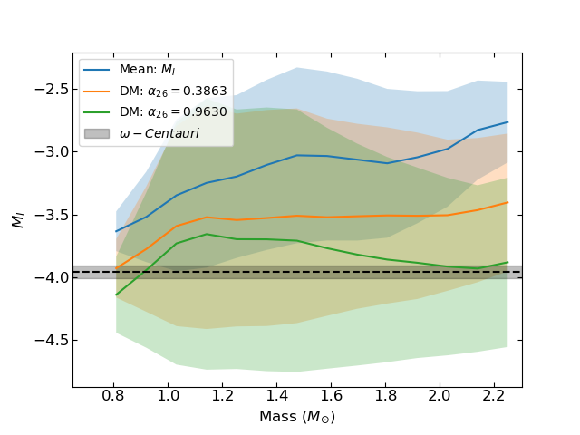
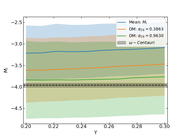
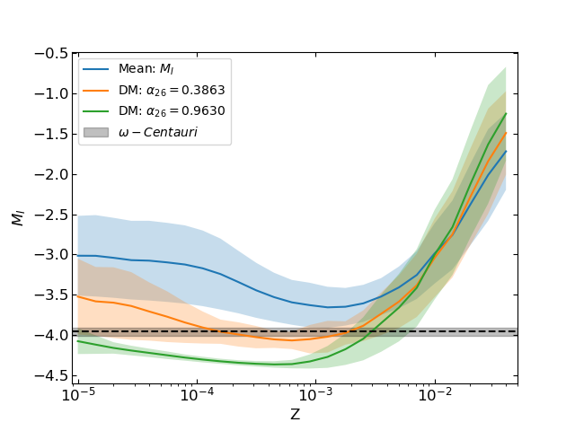
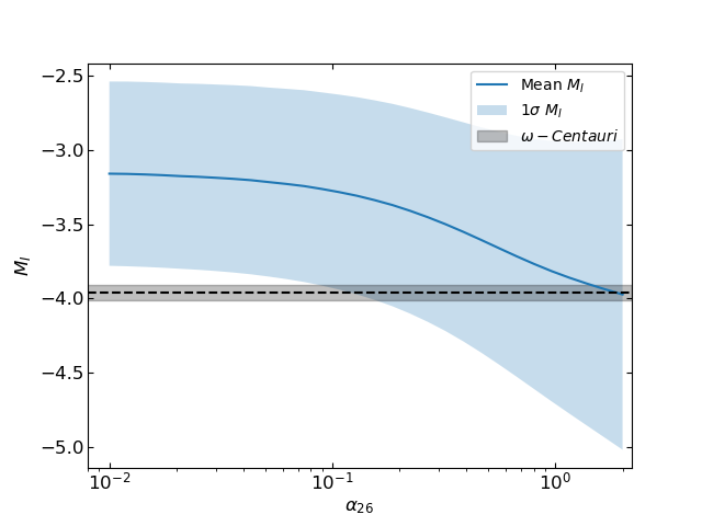
Figure 1: Variation in the TRGB $M_{I}$ using the $\omega$-Centauri color-correction with varying parameters indicated in the subfigures. The mean $M_{I}$ in each bin was found by averaging over the other parameters. The shaded error bands show the 1$\sigma$ deviation from the mean in each bin. The dark band represents the calibration of $M_{I}$ reported by [19].

We ran a grid of 116,250 models with varying initial mass $M$, helium abundance $Y$, metallicity $Z$, and $\alpha_{26}$. The models were evolved from the pre-main-sequence to the onset of the Helium flash (defined as the point where the power from helium burning exceeds $10^{6}$ ergs/s). We modified a version of the stellar structure code – Modules for Experiments in Stellar Astrophysics (MESA) version 12778 [20, 21, 22, 23, 24, 25] to account for axion losses by modifying the neutrino loss rate i.e., we treated axions as another form of neutrino loss. The parameters were varied over the ranges $0.7{\rm M}_{\odot}\leq M\leq 2.25{\rm M}_{\odot}$, $0.2\leq Y\leq 0.3$, $10^{-5}\leq Z\leq 0.04$, and $10^{-2}\leq\alpha_{26}\leq 2$. This grid was combined with 3,750 models from the SM grid simulated by [26] (which has identical input physics parameters) to extend the range of $\alpha_{26}$ to zero. The parameter ranges reflect the parameter space that will undergo a He flash (in $M$, $Y$, and $Z$) [27, 28], and the range where $\alpha_{26}$ has no effect on $M_{I}$ to the edge of where it would begin to affect stars on the main sequence. We used a linear grid spacing. We fix the stellar modelling parameters that correspond to input physics to fiducial values. In particular, we set the mixing length $\alpha_{MLT}=1.8$, use the MESA default nuclear reaction rates (a combination of NACRE and REACLIB [29, 30]), the mass loss on the red giant branch (RGB) to follow the Reimers prescription [31] with an efficiency parameter $\eta=0.1$, and we used the initial elemental abundances reported by [32] (GS98). Inlists containing all of our parameter choices can be found in our reproduction package [33]. We did not vary these other parameters because we had limited computing time for this preliminary study, and because we wanted to test the accuracy of the machine learning emulator before adding more parameters, which may have degraded its accuracy. Ultimately, our emulator was highly-accurate, and it is therefore likely that more parameters can be varied. We chose to focus on parameters that vary stochastically between stars due to mass and environment rather than parameters that are universal across all objects. The former class contribute to the variability of $M_{I}$ whereas the latter are a systematic offset.

The TRGB $M_{I}$ and its empirical error $\Delta M_{I}$ were calculated using the Worthey & Lee (WL) [36] bolometric correction code along with the $(V-I)$ colour and its associated empirical error $\Delta(V-I)$. The latter two quantities are needed because $M_{I}$ is dependent upon $(V-I)$, galaxy-dependent colour corrections must be applied to $M_{I}$. Each colour correction has a zero-point with respect to some $(V-I)$; therefore, the predicted $M_{I}$ value given by the ML must be converted to a prediction at the zero-point using the $(V-I)$ colour. The formulae for these (galaxy-dependent) corrections are given in Table 1. Our reproduction package includes a ML emulator (not used in this work) that predicts the luminosity $L$, the effective temperature $T_{\rm eff}$, the surface gravity $\log(g)$, and the iron abundance $[{\rm Fe}/{\rm H}]$. These can be used to calculate $M_{I}$ (and where appropriate $\Delta M_{I}$) using other bolometric corrections e.g., MARCS [37] or PHOENIX [38].

Some models in our grid did not reach the TRGB. These are models that either burn helium stably in the core before executing a helium shell flash (i.e., they do not exhibit a helium core flash and therefore do not contribute to the TRGB), or will not reach the TRGB in the current age of the universe. A small number of models failed to converge. These were not numerous enough to affect the ML and were therefore discarded. The results of our model grid that reach the TRGB in the current age of the universe and execute a core helium flash are compiled together in figure 1. The subfigures show the average value of $M_{I}$ and its standard deviation for a given bin of varying $M$, $Y$, $Z$, and $\alpha_{26}$. A band showing the calibration of $M_{I}$ in $\omega$-Centauri reported by [39] — from which [5] derived their strongest bound on $\alpha_{26}$ — is included for reference. The figure exemplifies the effects of degeneracies across parameter space. There is a weak correlation between $M_{I}$ with $Y$, however variation of the other parameters gives rise to more interesting features. Larger initial masses result in a dimmer $M_{I}$. This is because the extra mass is located in the envelope with the core mass being approximately constant. This extra mass results in a larger opacity, which causes the dimming. Turning to the metallicity, we find a maximum brightness at $Z\approx 10^{-3}$. The lack of metals at low metallicities reduces the opacity but also the rate of the CNO cycle compared with the pp-chains. The latter effect is dominant and hence the TRGB brightness is reduced. At high metallicities, the increase in the number of electrons increases the opacity by reducing the mean free path of photons in the stellar envelope, reducing the brightness. Looking at $\alpha_{26}$, the trend follows the explanation from above: as $\alpha_{26}$ increases, the Helium core mass at the point of Helium ignition increases leading to an overall increase in the brightness. Importantly, increasing $\alpha_{26}$ results in an increase in the number of models that are consistent with the empirical $M_{I}$ calibration. If one fixes $M$, $Y$, and $Z$ (or confines them to a narrow range) then increasing $\alpha_{26}$ will eventually lead to a TRGB $M_{I}$ that is not consistent with the empirical calibration. This highlights the important of exploring degeneracies over a wide range of parameter space. Narrow regions of $M$, $Y$, and $Z$ may not fit the data at fixed $\alpha_{26}$ but there may be other parameters for which consistency is achieved.

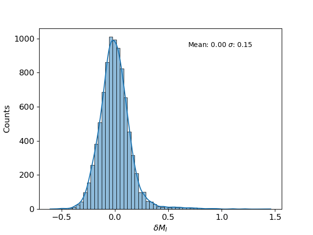
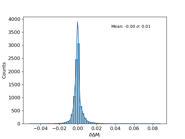
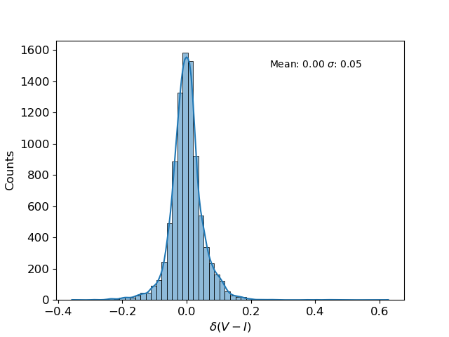
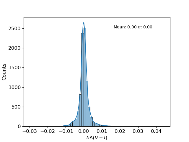
Figure 2: Error distributions for $M_{I}$, $\Delta M_{I}$, $(V-I)$, and $\Delta(V-I)$ from the ML regression. These distributions were calculated by subtracting the value of the ML prediction for each quantity from the value found by applying the WL code directly to the MESA outputs for each point in our grid. Note that helium flashing models and models that would not reach the helium flash in the age of the universe are excluded.

III Machine Learning Emulator

We trained a two component deep neural network (DNN) emulator on our grid of models described in the previous section using tensorflow [40] and keras [41]. All emulator algorithm components require the grid parameters $\{M,Y,Z,\alpha_{26}\}$ as their inputs. The first component was a classifier which accepted models which successfully reached the TRGB, and flagged those that either exhibited a helium shell flash or did not reach the TRGB in the current age of the universe. The other was a regression algorithm that predicts $M_{I}$ and $\Delta M_{I}$. Another regressor included in our reproduction package was trained that predicts luminosity $L$, effective temperature $T_{\rm eff}$, surface gravity $\log(g)$, and iron abundance $[{\rm Fe}/{\rm H}]$. This algorithm was less accurate than the other regressor. We include it for those interested in using different bolometric corrections.

We built our DNNs with an ADAM [42] optimizer and hand tuned our hyperparameters to optimize the network training. Both algorithms were trained using an 80%/10%/10% split between training, validation, and testing data. However, the classifier training set was resamppled using the Synthetic Minority Oversampling Technique (SMOTE) [44] to rebalance the training data which results in a more accurate emulator [45]. An unbalanced dataset can bias the network to labelling more objects as the more populous class while achieving similar levels of accuracy. The classification algorithm has an accuracy of 99.2% and a cross-entropy loss of 0.023. The regression algorithm predicts $M_{I}$, $\Delta M_{I}$, $(V-I)$, and $\Delta(V-I)$ with a mean squared error loss of $8.849\times 10^{-5}$ for input and output data that has been normalized between 0 and 1. Histograms of the residuals from the testing data for $M_{I}$, $\Delta M_{I}$, $V-I$, and $\Delta(V-I)$ are given in figure 2. The residual plots show that our errors are highly subdominant to the errors from the bolometric corrections, which have an average error of $\sim 0.1$ mag.

IV Constraining The Axion-Electron Coupling

In this section, we attempt to constrain $\alpha_{26}$ by using an MCMC sampler to compare the theoretical value of $M_{I}$ predicted by our ML emulator trained in section III with the calibrated values in the LMC, NGC 4258, and $\omega$-Centauri listed in table 1.

We performed the MCMC analysis using the emcee package [46] assuming uniform priors on $M$, $Y$, $Z$, and $\alpha_{26}$ with ranges $0.7{\rm M}_{\odot}\leq M\leq 2.25{\rm M}_{\odot}$, $0.2\leq Y\leq 0.3$, $10^{-5}\leq Z\leq 10^{-2}$, and $0<\alpha_{26}\leq 2$. The MCMC used the ML classification algorithm to assign a zero likelihood to models which do not successfully core helium flash within the age of the universe. The log-likelihood function was taken to be Gaussian i.e.,

$$\ln{\mathcal{L}}=-\frac{1}{2}\left[\left(\frac{M_{I,\textrm{obs}}-f(\textrm{ML}(\theta)_{I},\textrm{ML}(\theta)_{(V-I)})^{2}}{\sigma_{\textrm{tot}}}\right)^{2}\right.\\ +\left.~{}\ln(2\pi\sigma_{\textrm{tot}}^{2})\vphantom{\sum^{N}_{i=1}}\right],$$ (1)

where $M_{I,\textrm{obs}}$ is the observed I Band calibration, ML$(\theta)_{I}$ and ML$(\theta)_{(V-I)}$ are the ML predictions for $M_{I}$ and $(V-I)$ for a given set of parameters $\theta$, and $f(M_{I},(V-I))$ is the empirical calibration given in Table 1 for each galaxy. $\sigma_{\textrm{tot}}$ is given by

$$\sigma_{\textrm{tot}}^{2}=\sigma_{\textrm{obs}}^{2}+\sigma_{f}^{2},$$ (2)

where $\sigma_{\textrm{obs}}$ is the error on the empirical I band calibration and the error $\sigma_{f}$ in the calibration $f$ is given by

$$\sigma_{f}\approx\left|\frac{\partial f}{\partial M_{I}}\right|^{2}\Delta{M_{I}}^{2}+\left|\frac{\partial f}{\partial(V-I)}\right|^{2}\Delta{(V-I)}^{2}+\\ 2\left|\frac{\partial f}{\partial M_{I}}\right|\left|\frac{\partial f}{\partial(V-I)}\right|\Delta{M_{I}}\Delta{(V-I)}\rho_{M_{I}(V-I)},$$ (3)

where $M_{I}$ and $(V-I)$ are the ML predictions for the I band magnitude; $\Delta M_{I}$ and $\Delta{(V-I)}$ are their associated empirical errors from the bolometric corrections; and $\rho_{M_{I}(V-I)}$ is the correlation between $M_{I}$ and $(V-I)$ which was taken to be the covariance of the two variables from the full simulation dataset.

We accounted for the error in the ML by randomly drawing from the distributions in Figure 2 and adding them to the predictions from the ML emulator for each $\theta$, similar to the procedure in [47]. These errors are highly subdominant to the errors on the calibration and the bolometric correction but we included them for completeness. We performed MCMC analyses using the calibrations in the LMC [17]; NGC 4258 [18]; and $\omega$ Centauri [39], targets which have recent empirical calibrations that were adjusted by [5]. The system calibrations are summarized in Table 1. The results of the MCMC for $\omega$-Centauri are summarized in Figure 3. The corner plots for the other systems we studied are visually similar and are included in figures 5, 6 for the LMC and NGC 4258 in Appendix B. We determined that the chains had converged when the integrated autocorrelation time $\tau$ was less than 0.1% the length of the chain and that it had changed by less than 1% over the previous 10,000 points [48, 49]. We found that the MCMC converged within 120,000 steps but we allowed it to continue to 500,000 to ensure that the walker was no longer influenced by its starting location. We discarded half of the samples as burn-in.

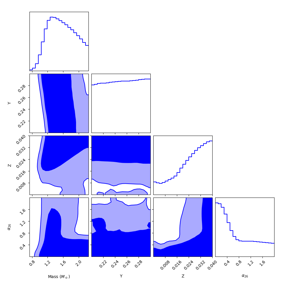
Figure 3: Posterior distributions of each parameter for the $\omega$-Centauri calibration of $M_{I}$. Both the 2D and marginalized posteriors are shown. The contours represent the 68% and 95% confidence intervals.

The mass, the helium abundance, and the metallicity are unconstrained within parameter space. The explanation for this result is explained in figure 1. The majority of parameter space for all three quantities intersect the empirical calibration within 1 standard deviation for the values of $\alpha_{26}$ shown. The posterior for $\alpha_{26}$ is dominated by its priors — the parameter is completely unconstrained. This too can be understood by examining figure 1. There are large regions of $M$, $Z$, and $Y$ that are consistent with the empirical $M_{I}$ calibration for all values of $\alpha_{26}<2$. Examining the 2D contours in figure 3 (and the bottom left panel of figure 1), one can see that the region of maximum likelihood at high $\alpha_{26}\gtrsim 0.8$ corresponds to super-solar metallicity with $Z\gtrsim 0.03$, implying that if one considers $\alpha_{26}\gtrsim 0.8$ viable then the metallicity in $\omega$-Centauri is super-solar. It is possible that other observations of $\omega$-Centauri could be used to provide a constraint on the metallicity that could then be used as a prior in our analysis and constrain $\alpha_{26}$. In a forthcoming publication [50], we will show that the preference for high-$Z$ is driven by our fiducial choice of the mixing length, and that higher values $\alpha_{\rm MLT}\sim 2$ give a maximum likelihood metallicity that is solar/sub-solar. Our conclusions are therefore robust to such caveats, but we comment that extending our analysis to vary the mixing length would be interesting in light of this. Our analyses of NGC 4258 and the LMC yielded similar results.

For $\alpha_{26}=0$ there is only a narrow range of parameter space that is consistent with the empirical calibration. At higher $\alpha_{26}$ this range is no longer consistent with the calibration so if one were to confine oneself to this region one would eventually find a constraint. But, if instead one lets $M$, $Y$, and $Z$ vary simultaneously, then there is in fact a larger region of parameter space that is consistent with the data, and therefore no meaningful bound can be placed. The novelty of our work lies in using the ML emulator to enable MCMC, and hence such a simultaneous variation, for the first time.

Previous works e.g., [8, 5, 51] found strong bounds on $\alpha_{26}$, the strongest being $\alpha_{26}<0.134$ (95% C.L.) coming from the $\omega$-Centauri $M_{I}$ calibration [5]. The adopted theoretical uncertainty on $M_{I}$ were those of [8], who modeled the TRGB in the globular cluster M5. The uncertainty reported by [8] is significantly smaller than the variation in $M_{I}$ we find when varying our parameters. This is because, despite varying more parameters than us, [8] only varied them over a narrow range (see their table 4). Their reasoning was that other independent bounds can place tight constraints on some input parameters e.g., age estimators can bound the mass of the stars at the TRGB [52] and spectroscopic measurements of red giant branch stars can measure the metallicity [53]. Applying these bounds is tantamount to imposing a very strong prior on the stellar modeling parameters in our framework.

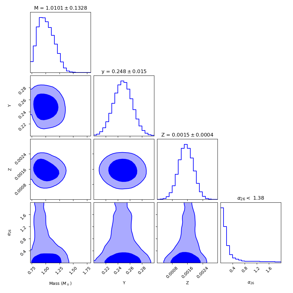
Figure 4: Same as 3, but using the Gaussian priors $M=0.820\pm 0.025{\rm M}_{\odot}$, $Y=0.245\pm 0.015$, and $Z=00136\pm 0.00035$, from [7] and [8]. The titles on the marginalized posteriors represent the means and standard deviations for $M$, $Y$, and $Z$. For $\alpha_{26}$, the title represents the 68% confidence limit. The posteriors indicate a return of the priors in all but $\alpha_{26}$. State what the contours are here

The measurements used to derive these priors are highly uncertain. The mass prior corresponds to the range of masses that reach the TRGB in 13.8 Gyr (the age of the universe) but different age estimates give values in the range $10.6\pm 0.8$ to $13.5\pm 1.0$ Gyr for M5 [54, 55, 56, 57] and a $2-4$ Gyr spread in stellar ages for $\omega$-Centauri [58]. Furthermore, the masses of stars that sit at the TRGB depend strongly on the metallicity. This was chosen based on measurements of [Fe/H] and [$\alpha$/Fe] that are then used as inputs to isochrone fitting formulas to estimate the metallicity. Different groups report a large spread in [Fe/H] ($-1.12$ to $-1.45$ for M5 [59, 60, 61, 54, 62, 56, 53, 63] and $-0.5$ to $-2.5$ for $\omega$-Centauri [64, 65]), and isochrone fitting alone is subject to large uncertainties that may not be accounted for [66, 67, 68] e.g., wind loss, opacity etc. Indeed, [67] note that these uncertainties can be accounted for using Bayesian methods such as ours, and advocate for such an approach. A large axion-electron coupling can alter the isochrones, providing an extra source of uncertainty. Additionally, there is no guarantee that the stars at the TRGB have metallicity equal to these measurements. Indeed, as an example, studies of the LMC have found that some objects have significantly different metallicites to the measured galactic metallicity [69, 70]. Finally, we note that priors should be imposed on a system-by-system basis since the targets of this (and previous) works will differ in age and composition from M5, especially in the LMC where the metallicity is typically reported as $Z\sim 0.008$ [71]. In light of these large uncertainties, we advocate for our data-driven approach where the uncertainties are constrained simultaneously with any new physics.

To investigate this further, we ran additional MCMCs using the three empirical calibrations listed in table 1 taking Gaussian priors on $M$, $Y$, and $Z$ with means and standard deviations equal to the central value and variation given in table 4 of [7], which were the same used to constrain $\alpha_{26}$ in [8]. An example is shown in figure 4. The MCMC recovered the priors we imposed, suggesting that these narrow priors are too restrictive, and that the empirical calibrations are not adding any constraining power for the stellar parameters. We obtain a bound $\alpha_{26}<1.38$ at the 95% confidence level, an order of magnitude larger than [5], who obtain $\alpha_{26}<0.134$. Thus we see that accounting for degeneracies by simultaneously varying stellar and new physics parameters with MCMC sampling weakens the constraints, even when tight priors are imposed, although we note that our fixed stellar parameters (e.g., mixing length) differ from those used by [5], as does our stellar structure code, so the systematic offset due to this may account for part of the discrepancy. Since the tight priors do not allow the stellar parameters to vary significantly, increasing $\alpha_{26}$ results in an $M_{I}$ that is brighter than the empirical calibration, leading to a bound on $\alpha_{26}$. This bound hinges crucially upon arbitrary choices for which competing measurements to take as priors, and errors on independent estimates of the stellar input physics being both accurately assessed and independent of the presence of axions.

V Discussion and Conclusions

In this section we discuss the implications of our results, potential applications of our methodology to other stellar tests of new physics, discuss caveats and the limitations of our method, and conclude.

V.1 Opening of the Axion-Electron Parameter Space

Our results have opened the parameter space $\alpha_{26}\leq 2$ which was previously believed to be constrained. Our grids do not extend to $\alpha_{26}>2$, so we are unable to make any definitive statements about this region of parameter space. We do make two comments. First, our result that $\alpha_{26}\leq 2$ is unconstrained does not imply that the region $\alpha_{26}>2$ is constrained. One would need to extend our grid to larger $\alpha_{26}$ and use this to extend the range of validity of the ML emulator to find the region excluded by TRGB empirical $M_{I}$ calibrations. This would be an interesting topic for future work. Second, it is highly likely that large regions of the parameter space $\alpha_{26}>2$ are viable. The marginalized posterior is flat for $\alpha_{26}\approx 2$, and, as can be seen in figure 1 (panel (c) specifically), there are many high-$Z$ models that are dimmer than the empirical calibration, even when $\alpha_{26}$ is large. One would need to increase $\alpha_{26}$ to the point where there are all brighter than the empirical calibration before $\alpha_{26}$ can be constrained.

The opening of the axion-electron parameter space has important implications for both stellar and terrestrial searches for axions. First, with the viable region of parameter space enlarged, it is possible that axions could be detected using other astrophysical probes (subject to the caveat that degeneracies and uncertainties with stellar physics should be accounted for in a similar manner to this work, see below). The region of parameter space we have opened is accessible to terrestrial dark matter direct detection chambers e.g., XENONnT [72], raising the tantalizing possibility that these experiments could detect axions.

V.2 Application to Other Stellar Tests of New Physics

There are no astrophysical systems that are free from degeneracies and uncertainties. Our work has highlighted the paramount importance of fully accounting for these when using astrophysical systems as probes of physics beyond the standard model. Our results indicate that a large range of values of the axion-electron coupling ostensibly believed to be excluded are in fact not. It is therefore highly likely that other astrophysical tests of new physics will be significantly weakened once stellar degeneracies and uncertainties are accounted for by varying them simultaneously with the new physics parameters in MCMC analyses. As discussed above, an accurate assessment of the stellar bounds is critical for complementary experimental searches.

The methods we have developed here could be applied to reevaluate the bounds obtained using other stellar tests of axions e.g., horizontal branch stars [73, 74] the white dwarf luminosity function [75, 76], pulsating white dwarfs [77], black hole population statistics [78, 79, 80, 81, 82, 83, 84], and Cepheid stars [85]. Another application would be to reevaluate the stellar bounds on other new physics models such as hidden photons, and theories where the neutrino has a large magnetic dipole moment. We expect all these bounds to be significantly weakened once stellar degeneracies and uncertainties are accounted for.

V.3 Limitations of Our Study

Our work is a preliminary study and, as such, is subject to some caveats and limitations. First, we only varied the mass, initial helium abundance, and initial metallicity of the stars we simulated; we held the stellar input physics such as nuclear reaction rates, mixing length, and neutrino energy loss rate fixed. These are known to be equally large sources of uncertainty [11, 86]. We made this choice for two reasons. The first is computational resources. Our grid took 1.23 million CPU hours to complete. Varying the four extra parameters (there are two important nuclear reaction rates) controlling the physics mentioned above (eight parameters in total) would take approximately 2.6 billion CPU hours. More efficient algorithms for sampling parameter space e.g., Latin hypercube sampling or active learning [87] would aid in decreasing the number of models needed per parameter. Second, it is likely that the accuracy of the ML emulator will be degraded by adding additional parameters. It is important that the errors in our constraint (or lack thereof) is due to experimental errors and not the ML error. For this reason, we chose to focus on the minimal number of parameters needed to produce physically reasonable variations to ensure an accurate emulator. We remark that varying additional stellar physics parameters can only act to increase the uncertainties on $\alpha_{26}$, so the conclusions of this work would only be strengthened if we were to include them. We note that including them is important if one wishes to place a new TRGB bound on $\alpha_{26}$ rather than open up the parameter space as we have done here.

The second caveat is that we have assumed that the TRGB I band magnitude is due solely to the brightest star. In practice, $M_{I}$ is calibrated using edge detection techniques (e.g., [88]) applied to the color-magnitude diagram. We made this choice to enable a comparison with previous works, which make the same assumption [10, 5]. We note that our emulator could be used to make theoretical predictions found using the same method as the empirical calibration. In particular, one could use our emulator to simulate a mock color-magnitude diagram by drawing $M$, $Y$, and $Z$ from some reasonable distribution for the specific system under study then apply the same edge-detection techniques to extract $M_{I}$ as a function of $(V-I)$ i.e., the zero-point and color-correction can be theoretically-predicted. One could even MCMC over these mock diagrams.

The final caveat is that our analysis includes statistical errors but not systematic. We have made specific choices for the input physics, including discrete choices such as elemental abundances, choice of bolometric corrections, and choice of stellar structure code. Furthermore, MESA may be missing physics such as three-dimensional processes. All of these act as a source of systematic uncertainty. It is unlikely that a different choice of code, input physics, or bolometric corrections will change our conclusions. Changing code is simply a systematic offset while different input physics and bolometric corrections have errors comparable to those we adopted in this work. It would be interesting to investigate the effects of varying these choices.

V.4 Conclusions

In this work we have presented a novel method for constraining physics beyond the standard model using stars that fully accounts for uncertainties and degeneracies due to stellar physics. Focusing on tip of the red giant branch bounds on the axion-electron coupling, we simulated a grid of 116,250 stellar models varying initial mass, helium abundance, and metallicity that we used to train a machine learning emulator to predict the I band magnitude (and errors due to bolometric corrections) as a function of these parameters. This was then used in a Markov Chain Monte Carlo analysis to compare with empirical calibrations. The novelty of our method lies in substituting the stellar structure code with our emulator in the MCMC. The long run-times of stellar structure codes (hours) is a major barrier to using MCMC to compare their predictions with data. Our emulator evaluates in milliseconds.

We found that once stellar uncertainties are accounted for, the data does not place any meaningful constraints on the axion-electron coupling when $\alpha_{26}\leq 2$. Our grid does not extend to $\alpha_{26}>2$ so we are unable to make any definitive statements about this region but, given the flat posterior we found, it is highly likely that larger values of $\alpha_{26}$ are viable. Our results have opened up a large region of parameter space that was previously believed to be excluded. This region is accessible to current and planned terrestrial dark matter direct detection chambers. It is highly likely that the bounds on new physics deriving from other stellar probes will be similarly weakened once degeneracies are fully accounted for. The methodology we have presented can be applied to these tests in a straightforward manner. Doing so is of paramount importance for determining the viable parameter space of theories beyond the Standard Model.

Software

MESA version 12778, MESASDK version 20200325, Worthey and Lee Bolometric Correction Code [36], NumPy version 1.22.3 [89] Pandas version 1.4.3 [90, 91], Matplotlib version 3.5.1 [92], Tensorflow version 2.4.1 [40, 41], corner version 2.2.1 [93], emcee version 3.1.2 [46].

Appendix A Axions and Implementation into MESA

The Lagrangian for the axion $a$ coupled to electrons is

$$\mathcal{L}=-ig_{ae}a\bar{\psi}_{e}\gamma_{5}\psi_{e}-\frac{1}{2}m_{a}^{2}a^{2},$$ (4)

where $g_{ae}$ is the (dimensionless) axion-electron coupling. It is common to work with the $\mathcal{O}(1)$ quantity $\alpha_{26}=10^{26}g^{2}_{ae}/4\pi$, which we adopt in this work. Other axion couplings to standard model fields are allowed but are not relevant for this study.

The rate of energy loss per unit time per unit mass due to the interaction in equation (4) is [10]

$$Q_{ae}=Q_{sC}+(Q_{b,ND}^{-1}+Q_{b,D}^{-1})^{-1},$$ (5)

where $Q_{sC}$ is the loss from semi-Compton scattering, $Q_{b,ND}$ is the non-degenerate bremmstrahlung loss, and $Q_{b,D}$ is the degenerate bremmstrahlung loss. Equation (5) is implemented into MESA as an additional source of energy loss due to neutrinos.

The semi-Compton scattering loss rate is given as

$$Q_{sC}\simeq 33\alpha_{26}Y_{e}T_{8}^{6}F_{\textrm{deg}}\frac{\textrm{erg}}{\textrm{g}\textrm{ s}},$$ (6)

where $Y_{e}=(Z/A)$ is the number of electrons per baryon, $T_{8}=T/10^{8}$K. $F_{\textrm{deg}}$ encodes Pauli-blocking due to electron degeneracy and can be approximated as

$$F_{\textrm{deg}}=\frac{1}{2}[1-\tanh f(\rho,T)]$$ (7)

with

$$f(\rho,T)=a\log_{10}\left[\frac{\rho}{\textrm{g}\textrm{ cm}^{-3}}\right]-b\log_{10}\left[\frac{T}{\textrm{K}}\right]+c$$ (8)

where $a=0.976$, $b=0.1596$, and $c=8.095$ per [78, 79]. The bremsstrahlung loss rate is broken into degenerate (D) and non-degenerate (ND) losses [10]

$$Q_{b,ND}\simeq 582\alpha_{26}\frac{\textrm{erg}}{\textrm{g}\textrm{ s}}\rho_{6}T^{5/2}F_{b,ND}$$ (9)

and

$$Q_{b,D}\simeq 10.8\sum_{i=\textrm{ions}}\frac{X_{i}Z_{i}}{A_{i}}\alpha_{26}\frac{\textrm{erg}}{\textrm{g}\textrm{ s}}T_{8}^{4}F_{b,D},$$ (10)

where $\rho_{6}=\rho/(10^{6}$ g/cm${}^{3})$, $X_{i}$ is the mass fraction per ion, $Z_{i}$ is the number of electrons per ion, and $A_{i}$ is the number of proton and neutrons per ion,

$$F_{b,D}=\frac{2}{3}\log(1+2\kappa^{-2})+\\ [(\kappa^{2}+2/5)\log(1+2\kappa^{-2})-2]\beta^{2}_{F}/3,$$ (11)

$$F_{b,ND}=\sum_{i=\textrm{ions}}\frac{X_{i}Z_{i}^{2}}{A_{i}}\sum_{i=\textrm{ions}}\frac{X_{i}Z_{i}}{A_{i}}\\ +\frac{1}{\sqrt{2}}\left(\sum_{i=\textrm{ions}}\frac{X_{i}Z_{i}}{A_{i}}\right)^{2},$$ (12)

and

$$\kappa^{2}=\frac{k_{s}^{2}}{2p_{f}^{2}}=\frac{4\pi\alpha_{EM}}{T}\sum_{i=\textrm{ions}}n_{i}Z_{i}^{2}+n_{i}Z_{i},$$ (13)

with $\beta_{F}=p_{F}/E_{F}$ where $p_{F}$ is the Fermi momentum and $E_{F}$ is the Fermi energy. In (13) above

$$n_{\textrm{ion}}=\rho_{ion}\frac{X_{ion}}{A_{ion}}\mathcal{N}_{A},$$ (14)

is the ion density of a particular ion.

Appendix B MCMC Results for Other Calibrations

In this Appendix we show the results of our MCMC analysis for NGC 4258 (figure 5) and the LMC (figure 6).

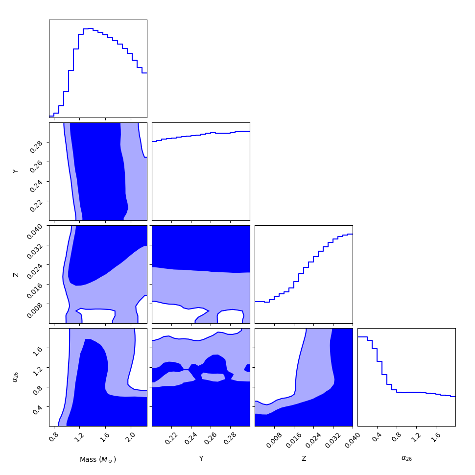
Figure 5: Same as 3 but for the LMC

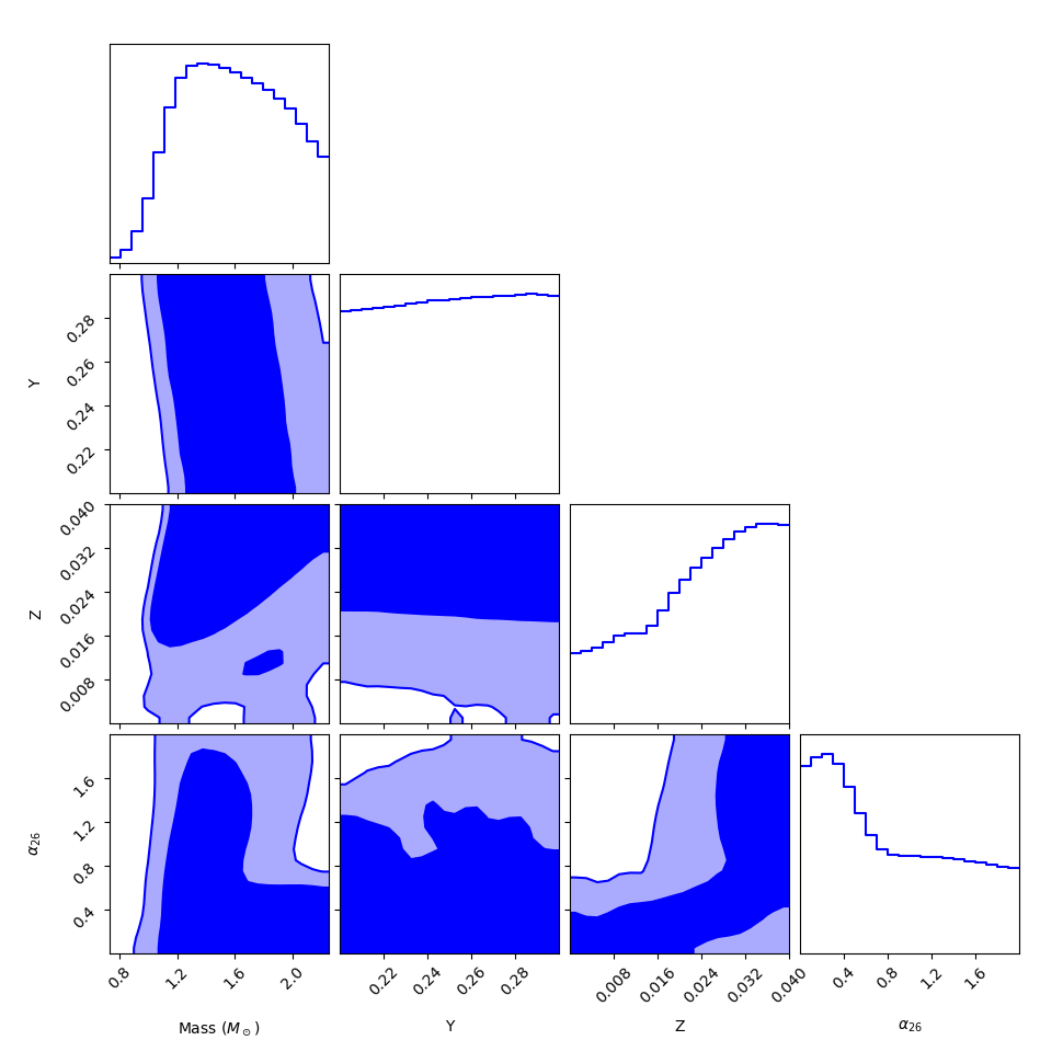
Figure 6: Same as 3 but for NGC 4258.

References

- Raffelt [1996] G. G. Raffelt, Stars as laboratories for fundamental physics : the astrophysics of neutrinos, axions, and other weakly interacting particles (1996).
- Ayala et al. [2015] A. Ayala, O. Straniero, M. Giannotti, A. Mirizzi, and I. Dominguez, Effects of Hidden Photons during the Red Giant Branch (RGB) Phase, in 11th Patras Workshop on Axions, WIMPs and WISPs (2015) pp. 189–192.
- Alonso-Álvarez et al. [2020] G. Alonso-Álvarez, F. Ertas, J. Jaeckel, F. Kahlhoefer, and L. J. Thormaehlen, Hidden photon dark matter in the light of XENON1T and stellar cooling, JCAP 2020, 029 (2020), arXiv:2006.11243 [hep-ph] .
- Lopes and Lopes [2021] J. Lopes and I. Lopes, Dark matter capture and annihilation in stars: Impact on the red giant branch tip, A&A 651, A101 (2021), arXiv:2107.13885 [astro-ph.SR] .
- Capozzi and Raffelt [2020] F. Capozzi and G. Raffelt, Axion and neutrino bounds improved with new calibrations of the tip of the red-giant branch using geometric distance determinations, PhRvD 102, 083007 (2020), arXiv:2007.03694 [astro-ph.SR] .
- Straniero et al. [2020] O. Straniero, C. Pallanca, E. Dalessandro, I. Domínguez, F. R. Ferraro, M. Giannotti, A. Mirizzi, and L. Piersanti, The RGB tip of galactic globular clusters and the revision of the axion-electron coupling bound, A&A 644, A166 (2020), arXiv:2010.03833 [astro-ph.SR] .
- Viaux et al. [2013a] N. Viaux, M. Catelan, P. B. Stetson, G. G. Raffelt, J. Redondo, A. A. R. Valcarce, and A. Weiss, Particle-physics constraints from the globular cluster M5: neutrino dipole moments, A&A 558, A12 (2013a), arXiv:1308.4627 [astro-ph.SR] .
- Viaux et al. [2013b] N. Viaux, M. Catelan, P. B. Stetson, G. G. Raffelt, J. Redondo, A. A. R. Valcarce, and A. Weiss, Neutrino and Axion Bounds from the Globular Cluster M5 (NGC 5904), PhRvL 111, 231301 (2013b), arXiv:1311.1669 [astro-ph.SR] .
- Arceo-Díaz et al. [2015] S. Arceo-Díaz, K. P. Schröder, K. Zuber, and D. Jack, Constraint on the magnetic dipole moment of neutrinos by the tip-RGB luminosity in -Centauri, Astroparticle Physics 70, 1 (2015).
- Raffelt and Weiss [1995] G. Raffelt and A. Weiss, Red giant bound on the axion-electron coupling reexamined, PhRvD 51, 1495 (1995), arXiv:hep-ph/9410205 [hep-ph] .
- Serenelli et al. [2017] A. Serenelli, A. Weiss, S. Cassisi, M. Salaris, and A. Pietrinferni, The brightness of the red giant branch tip. Theoretical framework, a set of reference models, and predicted observables, A&A 606, A33 (2017), arXiv:1706.09910 [astro-ph.SR] .
- Sakai [1999] S. Sakai, The Tip of the Red Giant Branch as a Population II Distance Indicator, in Cosmological Parameters and the Evolution of the Universe, Vol. 183, edited by K. Sato (1999) p. 48.
- Freedman et al. [2019] W. L. Freedman, B. F. Madore, D. Hatt, T. J. Hoyt, I. S. Jang, R. L. Beaton, C. R. Burns, M. G. Lee, A. J. Monson, J. R. Neeley, M. M. Phillips, J. A. Rich, and M. Seibert, The Carnegie-Chicago Hubble Program. VIII. An Independent Determination of the Hubble Constant Based on the Tip of the Red Giant Branch, ApJ 882, 34 (2019), arXiv:1907.05922 [astro-ph.CO] .
- Riess et al. [2021] A. G. Riess, S. Casertano, W. Yuan, J. B. Bowers, L. Macri, J. C. Zinn, and D. Scolnic, Cosmic Distances Calibrated to 1% Precision with Gaia EDR3 Parallaxes and Hubble Space Telescope Photometry of 75 Milky Way Cepheids Confirm Tension with CDM, ApJL 908, L6 (2021), arXiv:2012.08534 [astro-ph.CO] .
- Serenelli and Basu [2010] A. M. Serenelli and S. Basu, Determining the Initial Helium Abundance of the Sun, ApJ 719, 865 (2010), arXiv:1006.0244 [astro-ph.SR] .
- Saltas and Tognelli [2022a] I. D. Saltas and E. Tognelli, New calibrated models for the TRGB luminosity and a thorough analysis of theoretical uncertainties, MNRAS 10.1093/mnras/stac1546 (2022a), arXiv:2203.02499 [astro-ph.SR] .
- Yuan et al. [2019] W. Yuan, A. G. Riess, L. M. Macri, S. Casertano, and D. M. Scolnic, Consistent Calibration of the Tip of the Red Giant Branch in the Large Magellanic Cloud on the Hubble Space Telescope Photometric System and a Redetermination of the Hubble Constant, ApJ 886, 61 (2019), arXiv:1908.00993 [astro-ph.GA] .
- Jang and Lee [2017] I. S. Jang and M. G. Lee, The Tip of the Red Giant Branch Distances to Type Ia Supernova Host Galaxies. IV. Color Dependence and Zero-point Calibration, ApJ 835, 28 (2017), arXiv:1611.05040 [astro-ph.GA] .
- Freedman et al. [2020] W. L. Freedman, B. F. Madore, T. Hoyt, I. S. Jang, R. Beaton, M. G. Lee, A. Monson, J. Neeley, and J. Rich, Calibration of the Tip of the Red Giant Branch, ApJ 891, 57 (2020), arXiv:2002.01550 [astro-ph.GA] .
- Paxton et al. [2011] B. Paxton, L. Bildsten, A. Dotter, F. Herwig, P. Lesaffre, and F. Timmes, Modules for Experiments in Stellar Astrophysics (MESA), ApJS 192, 3 (2011), arXiv:1009.1622 [astro-ph.SR] .
- Paxton et al. [2013] B. Paxton, M. Cantiello, P. Arras, L. Bildsten, E. F. Brown, A. Dotter, C. Mankovich, M. H. Montgomery, D. Stello, F. X. Timmes, and R. Townsend, Modules for Experiments in Stellar Astrophysics (MESA): Planets, Oscillations, Rotation, and Massive Stars, ApJS 208, 4 (2013), arXiv:1301.0319 [astro-ph.SR] .
- Paxton et al. [2015] B. Paxton, P. Marchant, J. Schwab, E. B. Bauer, L. Bildsten, M. Cantiello, L. Dessart, R. Farmer, H. Hu, N. Langer, R. H. D. Townsend, D. M. Townsley, and F. X. Timmes, Modules for Experiments in Stellar Astrophysics (MESA): Binaries, Pulsations, and Explosions, ApJS 220, 15 (2015), arXiv:1506.03146 [astro-ph.SR] .
- Paxton et al. [2018] B. Paxton, J. Schwab, E. B. Bauer, L. Bildsten, S. Blinnikov, P. Duffell, R. Farmer, J. A. Goldberg, P. Marchant, E. Sorokina, A. Thoul, R. H. D. Townsend, and F. X. Timmes, Modules for Experiments in Stellar Astrophysics (MESA): Convective Boundaries, Element Diffusion, and Massive Star Explosions, ApJS 234, 34 (2018), arXiv:1710.08424 [astro-ph.SR] .
- Paxton et al. [2019] B. Paxton, R. Smolec, J. Schwab, A. Gautschy, L. Bildsten, M. Cantiello, A. Dotter, R. Farmer, J. A. Goldberg, A. S. Jermyn, S. M. Kanbur, P. Marchant, A. Thoul, R. H. D. Townsend, W. M. Wolf, M. Zhang, and F. X. Timmes, Modules for Experiments in Stellar Astrophysics (MESA): Pulsating Variable Stars, Rotation, Convective Boundaries, and Energy Conservation, ApJS 243, 10 (2019), arXiv:1903.01426 [astro-ph.SR] .
- Jermyn et al. [2022] A. S. Jermyn, E. B. Bauer, J. Schwab, R. Farmer, W. H. Ball, E. P. Bellinger, A. Dotter, M. Joyce, P. Marchant, J. S. G. Mombarg, W. M. Wolf, T. L. S. Wong, G. C. Cinquegrana, E. Farrell, R. Smolec, A. Thoul, M. Cantiello, F. Herwig, O. Toloza, L. Bildsten, R. H. D. Townsend, and F. X. Timmes, Modules for Experiments in Stellar Astrophysics (MESA): Time-Dependent Convection, Energy Conservation, Automatic Differentiation, and Infrastructure, arXiv e-prints , arXiv:2208.03651 (2022), arXiv:2208.03651 [astro-ph.SR] .
- Dennis and Sakstein [2023] M. Dennis and J. Sakstein, Machine Learning the Tip of the Red Giant Branch, arXiv e-prints , arXiv:2303.12069 (2023), arXiv:2303.12069 [astro-ph.GA] .
- Hansen et al. [2004] C. J. Hansen, S. D. Kawaler, and V. Trimble, Stellar interiors : physical principles, structure, and evolution (2004).
- Kippenhahn et al. [2013] R. Kippenhahn, A. Weigert, and A. Weiss, Stellar Structure and Evolution (2013).
- Angulo et al. [1999] C. Angulo et al., A compilation of charged-particle induced thermonuclear reaction rates, Nucl. Phys. A 656, 3 (1999).
- Cyburt et al. [2010] R. H. Cyburt, A. M. Amthor, R. Ferguson, Z. Meisel, K. Smith, S. Warren, A. e. Heger, R. D. Hoffman, T. Rauscher, A. e. Sakharuk, H. Schatz, F. K. Thielemann, and M. Wiescher, The JINA REACLIB Database: Its Recent Updates and Impact on Type-I X-ray Bursts, ApJS 189, 240 (2010).
- Reimers [1975] D. Reimers, Circumstellar absorption lines and mass loss from red giants., Memoires of the Societe Royale des Sciences de Liege 8, 369 (1975).
- Grevesse and Sauval [1998] N. Grevesse and A. J. Sauval, Standard Solar Composition, SSRv 85, 161 (1998).
- Dennis and Sakstein [2023] M. T. Dennis and J. Sakstein, Tip of the Red Giant Branch Bounds on the Axion- Electron Coupling Revisited, 10.5281/zenodo.7896061 (2023).
- Jimenez et al. [1996] R. Jimenez, P. Thejll, U. Jorgensen, J. MacDonald, and B. Pagel, Ages of globular clusters: a new approach, Mon. Not. Roy. Astron. Soc. 282, 926 (1996), arXiv:astro-ph/9602132 .
- Kipper and Jorgensen [1994] T. Kipper and U. G. Jorgensen, Chemical composition of the metal-poor carbon star HD 187216., A&A 290, 148 (1994).
- Worthey and Lee [2011] G. Worthey and H.-c. Lee, An Empirical UBV RI JHK Color-Temperature Calibration for Stars, ApJS 193, 1 (2011), arXiv:astro-ph/0604590 [astro-ph] .
- Gustafsson et al. [2008] B. Gustafsson, B. Edvardsson, K. Eriksson, U. G. Jørgensen, Å. Nordlund, and B. Plez, A grid of MARCS model atmospheres for late-type stars. I. Methods and general properties, A&A 486, 951 (2008), arXiv:0805.0554 [astro-ph] .
- Dotter et al. [2008] A. Dotter, B. Chaboyer, D. Jevremović, V. Kostov, E. Baron, and J. W. Ferguson, The Dartmouth Stellar Evolution Database, ApJS 178, 89 (2008), arXiv:0804.4473 [astro-ph] .
- Bellazzini et al. [2001] M. Bellazzini, F. R. Ferraro, and E. Pancino, A Step toward the Calibration of the Red Giant Branch Tip as a Standard Candle, ApJ 556, 635 (2001), arXiv:astro-ph/0104114 [astro-ph] .
- Abadi et al. [2015] M. Abadi, A. Agarwal, P. Barham, E. Brevdo, Z. Chen, C. Citro, G. S. Corrado, A. Davis, J. Dean, M. Devin, S. Ghemawat, I. Goodfellow, A. Harp, G. Irving, M. Isard, Y. Jia, R. Jozefowicz, L. Kaiser, M. Kudlur, J. Levenberg, D. Mané, R. Monga, S. Moore, D. Murray, C. Olah, M. Schuster, J. Shlens, B. Steiner, I. Sutskever, K. Talwar, P. Tucker, V. Vanhoucke, V. Vasudevan, F. Viégas, O. Vinyals, P. Warden, M. Wattenberg, M. Wicke, Y. Yu, and X. Zheng, TensorFlow: Large-scale machine learning on heterogeneous systems (2015), software available from tensorflow.org.
- Chollet et al. [2015] F. Chollet et al., Keras, https://keras.io (2015).
- Kingma and Ba [2014] D. P. Kingma and J. Ba, Adam: A Method for Stochastic Optimization, arXiv e-prints , arXiv:1412.6980 (2014), arXiv:1412.6980 [cs.LG] .
- Liashchynskyi and Liashchynskyi [2019] P. Liashchynskyi and P. Liashchynskyi, Grid Search, Random Search, Genetic Algorithm: A Big Comparison for NAS, arXiv e-prints , arXiv:1912.06059 (2019), arXiv:1912.06059 [cs.LG] .
- Chawla et al. [2011] N. V. Chawla, K. W. Bowyer, L. O. Hall, and W. P. Kegelmeyer, SMOTE: Synthetic Minority Over-sampling Technique, Journal of Artificial Intelligence Research , arXiv:1106.1813 (2011), arXiv:1106.1813 [cs.AI] .
- Sui et al. [2019] Y. Sui, X. Zhang, J. Huan, and H. Hong, Exploring data sampling techniques for imbalanced classification problems, in Fourth International Workshop on Pattern Recognition, Society of Photo-Optical Instrumentation Engineers (SPIE) Conference Series, Vol. 11198, edited by X. Jiang, Z. Chen, and G. Chen (2019) p. 1119813.
- Foreman-Mackey et al. [2013] D. Foreman-Mackey, D. W. Hogg, D. Lang, and J. Goodman, emcee: The MCMC Hammer, PASP 125, 306 (2013), arXiv:1202.3665 [astro-ph.IM] .
- McClintock et al. [2019] T. McClintock, T. N. Varga, D. Gruen, E. Rozo, E. S. Rykoff, T. Shin, P. Melchior, J. DeRose, S. Seitz, J. P. Dietrich, E. Sheldon, Y. Zhang, A. von der Linden, T. Jeltema, A. B. Mantz, A. K. Romer, S. Allen, M. R. Becker, A. Bermeo, S. Bhargava, M. Costanzi, S. Everett, A. Farahi, N. Hamaus, W. G. Hartley, D. L. Hollowood, B. Hoyle, H. Israel, P. Li, N. MacCrann, G. Morris, A. Palmese, A. A. Plazas, G. Pollina, M. M. Rau, M. Simet, M. Soares-Santos, M. A. Troxel, C. Vergara Cervantes, R. H. Wechsler, J. Zuntz, T. M. C. Abbott, F. B. Abdalla, S. Allam, J. Annis, S. Avila, S. L. Bridle, D. Brooks, D. L. Burke, A. Carnero Rosell, M. Carrasco Kind, J. Carretero, F. J. Castander, M. Crocce, C. E. Cunha, C. B. D’Andrea, L. N. da Costa, C. Davis, J. De Vicente, H. T. Diehl, P. Doel, A. Drlica-Wagner, A. E. Evrard, B. Flaugher, P. Fosalba, J. Frieman, J. García-Bellido, E. Gaztanaga, D. W. Gerdes, T. Giannantonio, R. A. Gruendl, G. Gutierrez, K. Honscheid, D. J. James, D. Kirk, E. Krause, K. Kuehn, O. Lahav, T. S. Li, M. Lima, M. March, J. L. Marshall, F. Menanteau, R. Miquel, J. J. Mohr, B. Nord, R. L. C. Ogando, A. Roodman, E. Sanchez, V. Scarpine, R. Schindler, I. Sevilla-Noarbe, M. Smith, R. C. Smith, F. Sobreira, E. Suchyta, M. E. C. Swanson, G. Tarle, D. L. Tucker, V. Vikram, A. R. Walker, J. Weller, and DES Collaboration, Dark Energy Survey Year 1 results: weak lensing mass calibration of redMaPPer galaxy clusters, MNRAS 482, 1352 (2019), arXiv:1805.00039 [astro-ph.CO] .
- Goodman and Weare [2010] J. Goodman and J. Weare, Ensemble samplers with affine invariance, Communications in Applied Mathematics and Computational Science 5, 65 (2010).
- Sokal [1997] A. Sokal, Monte Carlo Methods in Statisitical Mechanics: Foundations and New Algorithms, in Functional Integration: Basics and Applications, NATO ASI Series, edited by C. DeWitt-Morette, P. Cartier, and A. Folacci (Springer, Boston, MA, USA, 1997) pp. 131–192.
- [50] N. Franz, M. Dennis, and J. Sakstein, Tip of the Red Giant Branch Bounds on the Neutrino Magnetic Dipole Moment Revisited, in preparation .
- Di Luzio et al. [2020] L. Di Luzio, M. Fedele, M. Giannotti, F. Mescia, and E. Nardi, Solar Axions Cannot Explain the XENON1T Excess, PhRvL 125, 131804 (2020), arXiv:2006.12487 [hep-ph] .
- Dotter et al. [2010] A. Dotter, A. Sarajedini, J. Anderson, A. Aparicio, L. R. Bedin, B. Chaboyer, S. Majewski, A. Marín-Franch, A. Milone, N. Paust, G. Piotto, I. N. Reid, A. Rosenberg, and M. Siegel, The ACS Survey of Galactic Globular Clusters. IX. Horizontal Branch Morphology and the Second Parameter Phenomenon, ApJ 708, 698 (2010), arXiv:0911.2469 [astro-ph.SR] .
- Carretta et al. [2009] E. Carretta, A. Bragaglia, R. Gratton, V. D’Orazi, and S. Lucatello, Intrinsic iron spread and a new metallicity scale for globular clusters, A&A 508, 695 (2009), arXiv:0910.0675 [astro-ph.GA] .
- Sandquist et al. [1996] E. L. Sandquist, M. Bolte, P. B. Stetson, and J. E. Hesser, CCD Photometry of the Globular Cluster M5. I. The Color-Magnitude Diagram and Luminosity Functions, ApJ 470, 910 (1996), arXiv:astro-ph/9605101 [astro-ph] .
- Jimenez and Padoan [1998] R. Jimenez and P. Padoan, The Ages and Distances of Globular Clusters with the Luminosity Function Method: The Case of M5 and M55, ApJ 498, 704 (1998), arXiv:astro-ph/9701141 [astro-ph] .
- Marín-Franch et al. [2009] A. Marín-Franch, A. Aparicio, G. Piotto, A. Rosenberg, B. Chaboyer, A. Sarajedini, M. Siegel, J. Anderson, L. R. Bedin, A. Dotter, M. Hempel, I. King, S. Majewski, A. P. Milone, N. Paust, and I. N. Reid, The ACS Survey of Galactic Globular Clusters. VII. Relative Ages, ApJ 694, 1498 (2009), arXiv:0812.4541 [astro-ph] .
- Gontcharov et al. [2019] G. A. Gontcharov, A. V. Mosenkov, and M. Y. Khovritchev, Isochrone fitting of Galactic globular clusters - I. NGC 5904, MNRAS 483, 4949 (2019), arXiv:1812.06433 [astro-ph.GA] .
- Hughes and Wallerstein [2000] J. Hughes and G. Wallerstein, Age and Metallicity Effects in Centauri: StrÖmgren Photometry at the Main-Sequence Turnoff, AJ 119, 1225 (2000).
- Zinn and West [1984] R. Zinn and M. J. West, The globular cluster system of the Galaxy. III. Measurements of radial velocity and metallicity for 60 clusters and a compilation of metallicities for 121 clusters., ApJS 55, 45 (1984).
- Gratton et al. [1986] R. G. Gratton, M. L. Quarta, and S. Ortolani, The metal abundance of metal-rich globular clusters. II., A&A 169, 208 (1986).
- Sneden et al. [1992] C. Sneden, R. P. Kraft, C. F. Prosser, and G. E. Langer, Oxygen Abundances in Halo Giants. III. Giants in the Mildly Metal-Poor Globular Cluster M5, AJ 104, 2121 (1992).
- Kraft and Ivans [2003] R. P. Kraft and I. I. Ivans, A Globular Cluster Metallicity Scale Based on the Abundance of Fe II, PASP 115, 143 (2003), arXiv:astro-ph/0210590 [astro-ph] .
- D’Orazi et al. [2015] V. D’Orazi, R. G. Gratton, G. C. Angelou, A. Bragaglia, E. Carretta, J. C. Lattanzio, S. Lucatello, Y. Momany, A. Sollima, and G. Beccari, Lithium abundances in globular cluster giants: NGC 1904, NGC 2808, and NGC 362, MNRAS 449, 4038 (2015), arXiv:1503.05925 [astro-ph.SR] .
- Frinchaboy et al. [2002] P. M. Frinchaboy, J. Rhee, J. C. Ostheimer, S. R. Majewski, R. J. Patterson, W. Y. Johnson, D. I. Dinescu, C. Palma, and K. B. Westfall, The Metallicity Distribution Function of Centauri, in Omega Centauri, A Unique Window into Astrophysics, Astronomical Society of the Pacific Conference Series, Vol. 265, edited by F. van Leeuwen, J. D. Hughes, and G. Piotto (2002) p. 143, arXiv:astro-ph/0112169 [astro-ph] .
- Johnson et al. [2020] C. I. Johnson, A. K. Dupree, M. Mateo, I. Bailey, John I., E. W. Olszewski, and M. G. Walker, The Most Metal-poor Stars in Omega Centauri (NGC 5139), AJ 159, 254 (2020), arXiv:2004.09023 [astro-ph.SR] .
- Lachaume et al. [1999] R. Lachaume, C. Dominik, T. Lanz, and H. J. Habing, Age determinations of main-sequence stars: combining different methods, A&A 348, 897 (1999).
- Jørgensen and Lindegren [2005] B. R. Jørgensen and L. Lindegren, Determination of stellar ages from isochrones: Bayesian estimation versus isochrone fitting, A&A 436, 127 (2005).
- Huang et al. [2022] Y. Huang, T. C. Beers, C. Wolf, Y. S. Lee, C. A. Onken, H. Yuan, D. Shank, H. Zhang, C. Wang, J. Shi, and Z. Fan, Beyond Spectroscopy. I. Metallicities, Distances, and Age Estimates for Over 20 Million Stars from SMSS DR2 and Gaia EDR3, ApJ 925, 164 (2022), arXiv:2104.14154 [astro-ph.SR] .
- Marconi et al. [2013] M. Marconi, R. Molinaro, G. Bono, G. Pietrzyński, W. Gieren, B. Pilecki, R. F. Stellingwerf, D. Graczyk, R. Smolec, P. Konorski, K. Suchomska, M. Górski, and P. Karczmarek, The Eclipsing Binary Cepheid OGLE-LMC-CEP-0227 in the Large Magellanic Cloud: Pulsation Modeling of Light and Radial Velocity Curves, ApJL 768, L6 (2013), arXiv:1304.0860 [astro-ph.SR] .
- Desmond et al. [2021] H. Desmond, J. Sakstein, and B. Jain, Five percent measurement of the gravitational constant in the Large Magellanic Cloud, Phys. Rev. D 103, 024028 (2021), arXiv:2012.05028 [astro-ph.CO] .
- Glatt et al. [2010] K. Glatt, E. K. Grebel, and A. Koch, Ages and luminosities of young SMC/LMC star clusters and the recent star formation history of the Clouds, A&A 517, A50 (2010), arXiv:1004.1247 [astro-ph.GA] .
- Aprile et al. [2020] E. Aprile, J. Aalbers, F. Agostini, M. Alfonsi, L. Althueser, F. D. Amaro, V. C. Antochi, E. Angelino, J. R. Angevaare, F. Arneodo, D. Barge, L. Baudis, B. Bauermeister, L. Bellagamba, M. L. Benabderrahmane, T. Berger, A. Brown, E. Brown, S. Bruenner, G. Bruno, R. Budnik, C. Capelli, J. M. R. Cardoso, D. Cichon, B. Cimmino, M. Clark, D. Coderre, A. P. Colijn, J. Conrad, J. P. Cussonneau, M. P. Decowski, A. Depoian, P. di Gangi, A. di Giovanni, R. di Stefano, S. Diglio, A. Elykov, G. Eurin, A. D. Ferella, W. Fulgione, P. Gaemers, R. Gaior, M. Galloway, F. Gao, L. Grandi, C. Hasterok, C. Hils, K. Hiraide, L. Hoetzsch, J. Howlett, M. Iacovacci, Y. Itow, F. Joerg, N. Kato, S. Kazama, M. Kobayashi, G. Koltman, A. Kopec, H. Landsman, R. F. Lang, L. Levinson, Q. Lin, S. Lindemann, M. Lindner, F. Lombardi, J. Long, J. A. M. Lopes, E. López Fune, C. Macolino, J. Mahlstedt, A. Mancuso, L. Manenti, A. Manfredini, F. Marignetti, T. Marrodán Undagoitia, K. Martens, J. Masbou, D. Masson, S. Mastroianni, M. Messina, K. Miuchi, K. Mizukoshi, A. Molinario, K. Morâ, S. Moriyama, Y. Mosbacher, M. Murra, J. Naganoma, K. Ni, U. Oberlack, K. Odgers, J. Palacio, B. Pelssers, R. Peres, J. Pienaar, V. Pizzella, G. Plante, J. Qin, H. Qiu, D. Ramírez García, S. Reichard, A. Rocchetti, N. Rupp, J. M. F. Dos Santos, G. Sartorelli, N. Šarčević, M. Scheibelhut, J. Schreiner, D. Schulte, M. Schumann, L. Scotto Lavina, M. Selvi, F. Semeria, P. Shagin, E. Shockley, M. Silva, H. Simgen, A. Takeda, C. Therreau, D. Thers, F. Toschi, G. Trinchero, C. Tunnell, M. Vargas, G. Volta, H. Wang, Y. Wei, C. Weinheimer, M. Weiss, D. Wenz, C. Wittweg, Z. Xu, M. Yamashita, J. Ye, G. Zavattini, Y. Zhang, T. Zhu, J. P. Zopounidis, and X. Xenon Collaboration, Mougeot, Excess electronic recoil events in XENON1T, PhRvD 102, 072004 (2020), arXiv:2006.09721 [hep-ex] .
- Ayala et al. [2014] A. Ayala, I. Domínguez, M. Giannotti, A. Mirizzi, and O. Straniero, Revisiting the bound on axion-photon coupling from Globular Clusters, Phys. Rev. Lett. 113, 191302 (2014), arXiv:1406.6053 [astro-ph.SR] .
- Carenza et al. [2020] P. Carenza, O. Straniero, B. Döbrich, M. Giannotti, G. Lucente, and A. Mirizzi, Constraints on the coupling with photons of heavy axion-like-particles from Globular Clusters, Phys. Lett. B 809, 135709 (2020), arXiv:2004.08399 [hep-ph] .
- Miller Bertolami et al. [2014] M. M. Miller Bertolami, B. E. Melendez, L. G. Althaus, and J. Isern, Revisiting the axion bounds from the Galactic white dwarf luminosity function, JCAP 10, 069, arXiv:1406.7712 [hep-ph] .
- Dolan et al. [2021] M. J. Dolan, F. J. Hiskens, and R. R. Volkas, Constraining axion-like particles using the white dwarf initial-final mass relation, JCAP 09, 010, arXiv:2102.00379 [hep-ph] .
- Córsico et al. [2019] A. H. Córsico, L. G. Althaus, M. M. Miller Bertolami, and S. O. Kepler, Pulsating white dwarfs: new insights, Astron. Astrophys. Rev. 27, 7 (2019), arXiv:1907.00115 [astro-ph.SR] .
- Croon et al. [2021] D. Croon, S. D. McDermott, and J. Sakstein, Missing in axion: Where are XENON1T’s big black holes?, Physics of the Dark Universe 32, 100801 (2021), arXiv:2007.00650 [hep-ph] .
- Croon et al. [2020] D. Croon, S. D. McDermott, and J. Sakstein, Missing in Action: New Physics and the Black Hole Mass Gap, PhRvD , arXiv:2007.07889 (2020), arXiv:2007.07889 [gr-qc] .
- Sakstein et al. [2020] J. Sakstein, D. Croon, S. D. McDermott, M. C. Straight, and E. J. Baxter, Beyond the Standard Model Explanations of GW190521, Phys. Rev. Lett. 125, 261105 (2020), arXiv:2009.01213 [gr-qc] .
- Straight et al. [2020] M. C. Straight, J. Sakstein, and E. J. Baxter, Modified Gravity and the Black Hole Mass Gap, Phys. Rev. D 102, 124018 (2020), arXiv:2009.10716 [gr-qc] .
- Baxter et al. [2021] E. J. Baxter, D. Croon, S. D. McDermott, and J. Sakstein, Find the Gap: Black Hole Population Analysis with an Astrophysically Motivated Mass Function, Astrophys. J. Lett. 916, L16 (2021), arXiv:2104.02685 [astro-ph.CO] .
- Sakstein et al. [2022] J. Sakstein, D. Croon, and S. D. McDermott, Axion instability supernovae, Phys. Rev. D 105, 095038 (2022), arXiv:2203.06160 [hep-ph] .
- Croon and Sakstein [2022] D. Croon and J. Sakstein, Light Axion Emission and the Formation of Merging Binary Black Holes, arXiv e-prints , arXiv:2208.01110 (2022), arXiv:2208.01110 [astro-ph.HE] .
- Friedland et al. [2013] A. Friedland, M. Giannotti, and M. Wise, Constraining the Axion-Photon Coupling with Massive Stars, Phys. Rev. Lett. 110, 061101 (2013), arXiv:1210.1271 [hep-ph] .
- Saltas and Tognelli [2022b] I. D. Saltas and E. Tognelli, New calibrated models for the tip of the red giant branch luminosity and a thorough analysis of theoretical uncertainties, MNRAS 514, 3058 (2022b), arXiv:2203.02499 [astro-ph.SR] .
- Akira Rocha et al. [2022] K. Akira Rocha, J. J. Andrews, C. P. L. Berry, Z. Doctor, P. Marchant, V. Kalogera, S. Coughlin, S. S. Bavera, A. Dotter, T. Fragos, K. Kovlakas, D. Misra, Z. Xing, and E. Zapartas, Active Learning for Computationally Efficient Distribution of Binary Evolution Simulations, arXiv e-prints , arXiv:2203.16683 (2022), arXiv:2203.16683 [astro-ph.SR] .
- Müller et al. [2018] O. Müller, M. Rejkuba, and H. Jerjen, Distances from the tip of the red giant branch to the dwarf galaxies dw1335-29 and dw1340-30 in the Centaurus group, A&A 615, A96 (2018), arXiv:1803.02406 [astro-ph.GA] .
- Harris et al. [2020] C. R. Harris, K. J. Millman, S. J. van der Walt, R. Gommers, P. Virtanen, D. Cournapeau, E. Wieser, J. Taylor, S. Berg, N. J. Smith, R. Kern, M. Picus, S. Hoyer, M. H. van Kerkwijk, M. Brett, A. Haldane, J. F. del Río, M. Wiebe, P. Peterson, P. Gérard-Marchant, K. Sheppard, T. Reddy, W. Weckesser, H. Abbasi, C. Gohlke, and T. E. Oliphant, Array programming with NumPy, Nature 585, 357 (2020), arXiv:2006.10256 [cs.MS] .
- Wes McKinney [2010] Wes McKinney, Data Structures for Statistical Computing in Python, in Proceedings of the 9th Python in Science Conference, edited by Stéfan van der Walt and Jarrod Millman (2010) pp. 56 – 61.
- pandas development team [2020] T. pandas development team, pandas-dev/pandas: Pandas (2020).
- Hunter [2007] J. D. Hunter, Matplotlib: A 2D Graphics Environment, Computing in Science and Engineering 9, 90 (2007).
- Foreman-Mackey [2016] D. Foreman-Mackey, corner.py: Scatterplot matrices in python, The Journal of Open Source Software 1, 24 (2016).