Hunting muonic forces at emulsion detectors

Abstract

Only two types of Standard Model particles are able to propagate the $480\,$meters separating the ATLAS interaction point and FASER: neutrinos and muons. Furthermore, muons are copiously produced in proton collisions. We propose to use FASER$\nu$ as a muon fixed target experiment in order to search for new bosonic degrees of freedom coupled predominantly to muons. These muon force carriers are particularly interesting in light of the recent measurement of the muon anomalous magnetic moment. Using a novel analysis technique, we show that even in the current LHC run, FASER$\nu$ could potentially probe previously unexplored parts of the parameter space. In the high-luminosity phase of the LHC, we find that the improved sensitivity of FASER$\nu$2 will probe unexplored parameter space and may be competitive with dedicated search proposals.

1 Introduction

The Standard Model of particle physics (SM) successfully describes Nature in a wide range of energy scales. However, there is experimental evidence and strong theoretical arguments for the existence of new physics (NP) beyond the SM (BSM), see e.g. EuropeanStrategyforParticlePhysicsPreparatoryGroup:2019qin . New feebly interacting particles (FIPs) at the MeV–to–GeV mass range are well-motivated in many BSM scenarios and have recently received a lot of attention, both on the theoretical and experimental side Agrawal:2021dbo ; Lanfranchi:2020crw . One particular subset of FIPs are bosons with non-universal couplings to the SM fermions, which appear in various extensions of the SM Batell:2016ove ; Chen:2017awl ; Batell:2017kty ; Marsicano:2018vin .

Bosons which couple predominantly to muons, often referred to as muonic force carriers (MFCs), are motivated by the recent measurement of the muon anomalous magnetic moment, $(g-2)_{\mu}$ Bennett_2006 ; PhysRevLett.126.141801 . Comparing the experimental data to the data-driven SM prediction points to an anomaly, which can be explained by a weakly-coupled sub GeV MFC e.g. Pospelov:2008zw ; Jegerlehner:2009ry . However, recent lattice results Borsanyi:2020mff ; Alexandrou:2022amy ; Ce:2022kxy seem to suggest the data is in fact consistent with the SM. Moreover, a recent measurement of the $e^{+}e^{-}\to\pi\pi$ cross section even appears to alleviate the tension between the data-driven SM prediction and the experimental result CMD-3:2023alj .

On the other hand, it is possible that NP contributions to $(g-2)_{\mu}$ are suppressed due to cancellation at the quantum level. This was demonstrated in Balkin:2021rvh , where an approximate cancellation at the 1-loop level arises due to a global symmetry. This type of scenario provides a clear motivation for more direct, tree-level searches, such as the one proposed in this work.

Beyond the precision measurement of $(g-2)_{\mu}$, MFCs were targeted by direct searches in flavor factories such as BaBar BaBar:2016sci , Belle II Belle-II:2019qfb and NA62 Krnjaic:2019rsv ; NA62:2021bji , while vector MFCs were also probed by neutrino beam experiments CHARM-II:1990dvf ; CCFR:1991lpl ; Altmannshofer_2014 . In addition, there is a bound from supernova SN1987 Croon:2020lrf . Proposed experiments such as NA64_μ Chen:2017awl ; Chen:2018vkr ; Gninenko:2019qiv , M³ Kahn:2018cqs and proton beam dump Forbes:2022bvo can potentially probe unexplored regions of the MFC parameter space. An alternative approach is to maximize the NP reach of running experiments. For example, it was shown that the ALTAS experiment can probe the MFC parameter space via missing momentum measurements Galon:2019owl .

In this work, we present a novel method to search for MFCs using emulsion detectors as muon fixed targets. In particular, we estimate the sensitivity of FASER$\nu$ FASER:2019dxq ; FASER:2020gpr ; FASER:2021mtu , the front part of the running Forward Search Experiment (FASER) Feng_2018 ; FASER:2018ceo ; FASER:2018bac ; FASER:2018eoc , to the MFC parameter space. Neutrinos and muons are the only SM particles able to propagate the $480$ meters separating the ATLAS interaction point and FASER. The muons are produced in proton collisions, mostly as decay products or in secondary interactions between the collision products and the surrounding matter. Although most muons are deflected, an estimate of $N_{\mu}\sim 10^{9}$ muons with energy above $100\,\mathrm{GeV}$ are expected to reach FASER$\nu$ with $150\,\mathrm{fb}^{-1}$ integrated luminosity FASER:2018eoc . Using missing energy signatures, we estimate that MFC couplings as small as $10^{-3}-10^{-4}$ may be within reach in FASER$\nu$ and even smaller with FASER$\nu$2, which is expected to be installed at the LHC high luminosity (HL-LHC) stage. The sensitivity crucially depends on the background rejection efficiency, which must be carefully estimated in a dedicated detector study left for future work.

2 Simplified model

We consider a simplified model in which the muon is coupled to a light mediator $\chi=\{S,V\}$, with the following interaction Lagrangians,

$$\mathcal{L}_{S}=g_{S}\,S\,\bar{\mu}\mu\,\qquad\text{and}\qquad\mathcal{L}_{V}=g_{V}V_{\alpha}\,\bar{\mu}\gamma^{\alpha}\mu\,,$$ (1)

for a scalar and vector MFC, respectively, with the masses denoted by $m_{\chi}$. Pseudo scalar and axial vector interactions are expected to give similar results. The effective theory described by Eq. (1) can emerge as a low energy limit of a UV complete theory; for example scalar interactions can arise as a result of integrating out heavy leptons Krnjaic:2019rsv , while the vector interactions naturally arise in a spontaneously broken gauged $U(1)_{L_{\mu}-L_{\tau}}$ theory  He:1990pn ; Foot:1990mn ; PhysRevD.44.2118 .

Assuming $\chi$ is negligibly coupled to other SM constituents (e.g. the irreducible one-loop level coupling of $S$ to photons), we consider the case where it is either long-lived at the detector scale or decays invisibly. This scenario can arise naturally in the muonphillic case when $m_{\chi}<2m_{\mu}$, while above the di-muon threshold some more assumptions are required e.g. sizable decay rate to a dark sector. Either way, once scattered against a fixed-target $N$, some muons lose a fraction of their energy due to the 2-to-3 process,

$$N+\mu\to N+\mu+\chi\,,$$ (2)

while $\chi$ or its dark sector decay products escape the system without depositing any energy in the detector. Thus, $\chi$ can be searched for using missing-momentum signatures in FASER$\nu$, utilizing it as a muon-fixed-target experiment.

3 Method

FASER$\nu$ is an emulsion detector mounted in front of the FASER main detector. It is composed of 730 emulsion layers interleaved with 1.1 mm thick tungsten plates of area $S_{\text{FASER$\nu$}}=25\,\mathrm{cm}\times 30\,\mathrm{cm}$ FASER:2023zcr . As muons pass through FASER$\nu$, their track are measured by the emulsion layers. Throughout this work, we assume each layer provides only the position of the muon as it passes. In principle, due to the finite thickness of the emulsion layer and its structure, additional angular information can be deduced, which can potentially be harnessed to improve the analysis. We characterize each muon passing through FASER$\nu$ by two simple properties: (i) the ratio between the final and the initial muon energies, $\mathcal{R}_{fi}\equiv(E_{\mu})_{f}/(E_{\mu})_{i}$, and (ii) the largest scattering angle of the track, $\theta_{\mu}$, which characterizes the largest kink in the track. Large kinks are strongly correlated with large energy losses.

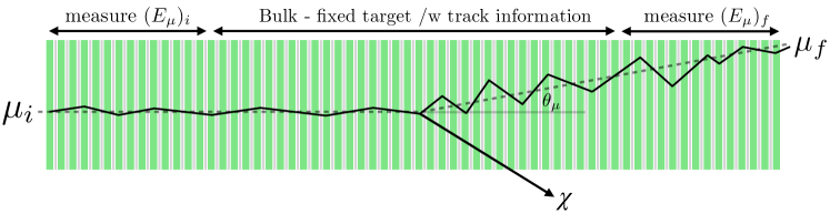
Figure 1: A sketch of a muon track at FASER$\nu$. The initial and final energies can be estimated using the MCS method (see Sec. 3.1), where we emphasize using the solid black lines that the MCS angles would generically increase after the muon losses energy. In practice, the MCS angles are $\mathcal{O}(1\,\text{mrad})$ and the muon tracks appear as straight lines (dashed).

To fully benefit from the layered structure of FASER$\nu$, we propose the detector acts as an instrumented target:

• The bulk of the detector supplies the target mass and is used as a fixed target for the incoming muon flux.

• Using the precise information about the positions of the muon as it propagates through the detector, the front and rear parts of FASER$\nu$ are used to measure the incoming and outgoing energies of the muon, respectively, using a method based on multiple Coulomb scattering (MCS), such as the one outlined in Sec. 3.1.

• The same spatial information can be used in the bulk of the detector in order to identify the position and magnitude of kinks in the track.

Our track characterization is summarized in a sketch shown in Fig. 1.

3.1 Muon energy reconstruction

Let us briefly review an MCS-based method for measuring a particle energy in an emulsion detector Kodama:2002dk ; OPERA:2011aa ; FASER:2019dxq . As charged particles pass through medium, they undergo a large number of elastic, small-angle Coulomb scatterings off nuclei. Due to the central limit theorem, the cumulative effects of the scatterings are normally distributed Bethe:1953va ; Scott:1963xw ; Motz:1964gpe . The MCS angle $\theta$ of an outgoing, unit-charge particle (relative to the incoming direction) with energy $E\gg m$ is approximately described by a Rayleigh distribution $\sim({\theta}/{\sigma^{2}_{\theta}})e^{-\theta^{2}/(2\sigma^{2}_{\theta})}$ with Lynch:1990sq

$$\sigma_{\theta}(X,E) \approx(0.136\,\text{mrad})\left(\frac{100\,\text{GeV}}{E}\right)\,\sqrt{{X}/{X_{0}}}\left[1+0.038\log\left(X/X_{0}\right)\right]\,,$$ (3)

where $X$ is the in-medium propagation distance and $X_{0}$ is the material radiation length. Thus, the typical single-layer, $X\sim 1.1\,\mathrm{mm}$, MCS angle in FASER$\nu$ for a 100 GeV muon is roughly $\sigma_{\theta}\sim 0.07\,$mrad, where we used $X_{0}^{W}=3.504\,\mathrm{mm}$ Workman:2022ynf . This is to be compared with the single-layer angular resolution in FASER$\nu$ of $\sigma_{\text{ang}}\sim 0.23$ mrad, where we used $\sigma_{\text{ang}}=\sqrt{2}\sigma_{\text{pos}}/X$ FASER:2019dxq , with $\sigma_{\text{pos}}=0.18\times 10^{-3}\,\mathrm{mm}$ AkiTalk the spatial resolution of the emulsion plate.

In practice, the muon energy is estimated by measuring linear displacements rather than angles, which are defined as follows. Consider three points along the track, denoted by $(x_{i},y_{i},z_{i})$ with $i=0,1,2$. The $z_{i}$’s are locations of emulsion plates such that $z_{2}-z_{1}=z_{1}-z_{0}\approx X$ (neglecting the width emulsion layer, to be reintroduced in Eq. (6)). The linear displacement in the $x$ coordinate is defined as

$$s_{x}\equiv(x_{2}-x_{1})-(x_{1}-x_{0})\,,$$ (4)

and similarly for the $y$ coordinate. Clearly $s_{x}=0\,(s_{y}=0)$ if the three points are on a line in the $x-z\,(y-z)$ plane. The variables $s_{x}$ and $s_{y}$ are independent random variables, which are normally distributed with the following standard deviation

$$\sigma_{s}(X,E)=\sqrt{\left[\sqrt{2/3}X\,\sigma_{\theta}(X^{\text{scat}},E)\right]^{2}+\left[\sqrt{6}\,\sigma_{\text{pos}}\right]^{2}}\,,$$ (5)

where

$$X^{\text{scat}}(X)\equiv\left(\frac{\Delta_{W}}{\Delta_{W}+\Delta_{\text{\tiny emu.}}}\right)X\,,$$ (6)

is the scattering length as a function of the physical propagation length $X$. The prefactor takes into account the fact that the finite-width emulsion layer is not a scattering medium. It is given by the ratio of the length of the scattering medium, i.e. $\Delta_{W}=1.1\,\mathrm{mm}$ of tungsten, and the physical propagation distance $\Delta_{W}+\Delta_{\text{\tiny emu.}}$ , where $\Delta_{\text{\tiny emu.}}=0.34\,\mathrm{mm}$ is the width of the emulsion plate. For a given track, Eq. (5) can be calculated for various values of $X$. The energy $E$ can then be inferred by performing a fit to the data.

The FASER collaboration reported an energy resolutions of $46\%$ and $57\%$ for $E=200\,\mathrm{GeV}$ and $1\,\mathrm{TeV}$, respectively, applying the MCS method using $100$ layers FASER:2019dxq . We analyzed simulated data at lower energies, which yielded similar results, for more details see App. A. By using a larger sample size of 400 (200 layers of independent $x,y$ displacements), the statistics-dominated energy uncertainty is reduced by about a factor of $\sim\sqrt{400/100}\sim 2$, namely $\Delta E/E\sim 20\%$.

An MCS-based method can also be used to determine $\theta_{\mu}$. First, we identify the region in the detector in which the muon lost its energy using a sliding window algorithm. The largest scattering angle measured in this region is strongly correlated with $\theta_{\mu}$, if the scattering angle is larger than the typical MCS angle and is above the angular resolution. This is usually the case for large energy losses, which as we discuss below, is the kinematic region of interest. In a preliminary study, we find that even a simple realization of this algorithm leads to a small reduction in signal efficiency, which can be made even smaller with optimization, e.g. by using machine learning. A detailed study is left for future work.

3.2 Signal

We calculated the cross-section for the coherent process of Eq. (2) (taking $N$ to be tungsten atoms) numerically using madgraph Alwall:2014hca for a range of MFC masses and initial muon energies, see Fig. 2. The cross section depends only weakly on the initial energy of the muon and decreases as expected for heavier MFC masses.

Figure 2: The cross-section of the process $N\mu\to N\mu\,\chi$ as a function of $m_{\chi}$ for $N=\text{W}$ and $\chi=S\,(V)$ left (right). Both cross section are plotted for $g_{S}=g_{V}=1$.

Each MFC emission event can be characterized by $\mathcal{R}_{fi}$ and $\theta_{\mu}$. As shown in Fig. 3, heavier MFC masses typically lead to larger scattering angles and energy loss, which are strongly correlated, see Fig. 4. Lighter MFC masses, on the other hand, lead to smaller scattering angles and energy loss and are increasingly SM-like. For comparison, we also plot the corresponding distributions from the main background due to bremsstrahlung, to be discussed below in Sec. 3.3.

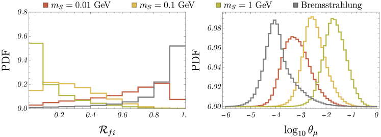
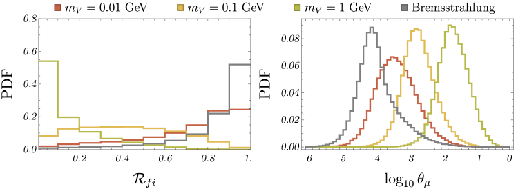
Figure 3: Signal $\mathcal{R}_{fi}$ and $\theta_{\mu}$ distributions for $(E_{\mu})_{i}=100$ GeV and three representative scalar (top) and vector (bottom) MFC masses, 0.01 GeV, 0.1 GeV and 1 GeV in red, yellow and green, respectively. For comparison, we plot the same distribution for our dominant background due to bremsstrahlung.

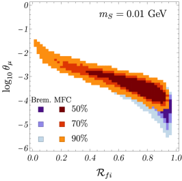
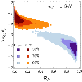
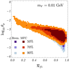
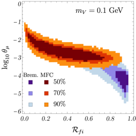
Figure 4: 2D probability density distribution $\{\mathcal{R}_{fi},\theta_{\mu}\}$ for $(E_{\mu})_{i}=100$ GeV and three representative scalar (top) and vector (bottom) MFC masses, 0.01 GeV (left), 0.1 GeV (center) and 1 GeV (right). For comparison, we plot the same distribution for our dominant background due to bremsstrahlung.

3.3 Background

The propagation of muons through matter has been studied in detail, see e.g. Workman:2022ynf . The main SM processes which contribute to the energy loss of the muon as it propagates through matter are, by probability order at small energy losses,

$$N+\mu\to\begin{cases}N+\mu+e^{-}+e^{+}&\text{(Pair production)}\\ N^{+}+\mu+e^{-}\;\;\;\;&\text{(Ionization)}\\ N+\mu+\gamma&\text{(Bremsstrahlung)}\\ N^{*}+\mu+...&\text{(Nuclear)}\end{cases}\,.$$ (7)

As the muon propagates through the tungsten layers, its total energy loss is typically an accumulation of a large number of scatterings due to the processes of Eq. (7). At $100\,$GeV, the average energy loss in tungsten is $\langle dE/dx\rangle=3.05\,\mathrm{MeV}\mathrm{cm}^{2}/\text{gr}$ Workman:2022ynf . Thus, the average energy loss at FASER$\nu$ would be $\langle\Delta E\rangle=4.97\,\mathrm{GeV}$ per muon.

Our main source of background are rare events in which the muon loses a large fraction of its energy due to a SM process. In order to study the background processes, we simulated $\sim 5\times 10^{6}$ muon tracks as they propagate through a simplified model of FASER$\nu$ using GEANT4 GEANT4:2002zbu ; Bogdanov:2006kr with various values for the initial energy. We associate each of the $\sim 5\times 10^{6}$ simulated tracks with one of the SM processes listed in Eq. (7) according to its single largest energy loss event during its propagation. This identification is useful for tracks in which a rare hard scattering occurred, while tracks with small energy losses, as explained above, are typically a result of many soft scatterings. We present the distribution of tracks in Table 1. The $\mathcal{R}_{fi}$ and $\theta_{\mu}$ probability distributions for each individual process are plotted in Fig. 5. The correlation between the kinematic variables can be seen in the density plots of Fig. 6. As expected, the vast majority of these scattering events generate small energy loss, $\Delta E\lesssim\langle\Delta E\rangle$, while the rare large energy loss events are dominated by bremsstrahlung.

	Pair	Ionization	Brems.	Nuclear	Total
# of tracks	$3.15\times 10^{6}$	$1.42\times 10^{6}$	$3.45\times 10^{5}$	$4.7\times 10^{4}$	$4.96\times 10^{6}$
Fraction	$0.63$	$0.29$	$0.07$	$0.009$	1.0

Table 1: Distribution of tracks according to the SM process responsible for the largest energy loss along the track. This distribution was calculated for initial muon energy of $100\,\mathrm{GeV}$. Note that at these high energies, the dependence of these rates on the initial muon energy is negligible.

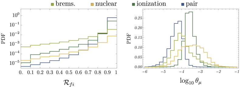
Figure 5: Background $\mathcal{R}_{fi}$ (left) and $\theta_{\mu}$ (right) distributions for bremsstrahlung (light green), nuclear (yellow), ionization (dark green) and pair production (blue) processes of Eq. (7) with $(E_{\mu})_{i}=100\,\mathrm{GeV}$. Note that the $\mathcal{R}_{fi}$ distributions are weighted according to the values in Table 1, such that the sum of all four curves is normalized to 1.

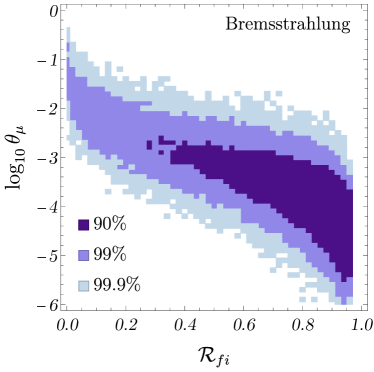
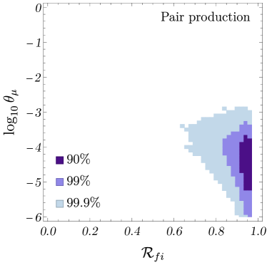
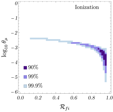
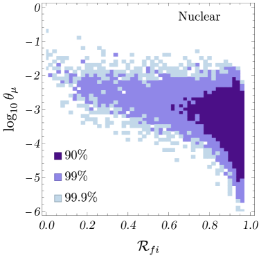
Figure 6: 2D probability density distribution $\{\mathcal{R}_{fi},\theta_{\mu}\}$ for bremsstrahlung, nuclear, ionization and pair production process shown in Eq. (7) with $(E_{\mu})_{i}=100$ GeV.

The background (BG) rejection for the three prompt SM processes, i.e. ionization, pair production and nuclear, quantifies the ability to detect energy depositions in the close vicinity of a given muon track. This can be done either by (1) finding a statistically significant excess of secondary particles around the muon track, or by (2) associating an emerging high-energy particle track to the muon track. The transverse length scale of EM showers comprised from secondary particles is given by the Molière radius, $r_{\text{\tiny M}}=9.3\,\mathrm{mm}$ in tungsten Workman:2022ynf . The other relevant scale is the average inter-track distance $r_{\text{track}}\sim\rho^{-1/2}$, where $\rho$ is the average track surface density. If $r_{\text{track}}\gg r_{\text{\tiny M}}$, the tracks are sufficiently separated such that each track can be treated in isolation and essentially all SM processes may be easily identified. Using Eq. (10), we estimate

$$\rho\sim\frac{N_{\mu}}{N_{\text{\tiny dev}}S_{\text{FASER$\nu$}}}\sim\frac{6.7\times 10^{4}}{\text{cm}^{2}}\left(\frac{20}{N_{\text{\tiny dev}}}\right)\left(\frac{\mathcal{L}}{150\,\text{fb}^{-1}}\right)\,,$$ (8)

where $N_{\text{\tiny dev}}$ is the number of emulsion film development during the run. We find that $r_{\text{track}}\sim 0.04~{}\text{mm}\ll r_{\text{\tiny M}}$. Therefore, identifying an excess of secondary particles could be challenging as it would have to be made on top of the pile-up generated by the surrounding tracks. Alternatively, one could try to identify single tracks of high-energy electrons and positrons emerging from a source muon track. These tracks typically emerge at length scales much smaller than the Molière radius and their identification is essentially limited by the spatial resolution of the emulsion track $\sigma_{\text{\tiny pos}}\ll r_{\text{track}}$.

Both approaches outlined above would prove to be more challenging for bremsstrahlung; any sign for the photon emission is expected to be displaced due to the propagation of the photon in matter. The probability of correctly associating a displaced energy deposition with a given track determines the bremsstrahlung BG rejection rate. Beyond the overall ability to detect excess energy deposition anywhere in the detector, the bremsstrahlung rejection rate depends on two additional factors: (1) the typical transverse distance travelled by the photon and (2) the density of relevant tracks, i.e. tracks which could be mistakenly associated with the emitted photon. The former factor depends on the propagation of photons in FASER$\nu$; the mean free path of photons in tungsten is $(9/7)X^{W}_{0}\sim 4.5\,\mathrm{mm}$, and the photon angle distribution peaks around $\theta_{\gamma}\sim{m_{\mu}}/{E_{\mu}}\sim 10^{-3}$, see App. B for more details. A naive estimation results in an average transverse displacement of $4.5\times 10^{-3}\,\mathrm{mm}$ for a $100\,\mathrm{GeV}$ muon, which is an order of magnitude smaller than $r_{\text{track}}$. However, photons emitted at larger angles are exponentially more likely to propagate a larger transverse distance, therefore a reliable modeling of the photon angle distribution at large angles is necessary. The second factor, the density of the relevant tracks, depends on the kinematic cuts and algorithms used. For example, the number of relevant tracks can be reduced by a factor of $\sim 10^{-2}-10^{-3}$ by considering only tracks for which a substantial energy loss was observed. The number of relevant tracks can be further reduced by considering only the tracks for which the energy loss occurred in the same region as the track in question. This reduction depends on the efficiency of the algorithm used to identify the energy loss region, such as the sliding window algorithm outlined above. We conclude that a significant fraction of bremsstrahlung events can expected to be vetoed by applying isolation criteria. Further rejection could be achieved by the detection of significant EM deposits (without necessarily requiring a complete photon reconstruction) and the use of kinematic characteristics. The proper development and optimization of this technique requires a detailed experimental study which is beyond the scope of this work.

4 Projected sensitivity

The expected luminosity per muon on a tungsten target of length $\Delta$ is given by

$$\frac{\mathcal{L}_{\text{eff}}}{N_{\mu}}=\left(\frac{\rho_{W}}{m_{\rm W}}\right)\Delta=5.1\times 10^{-15}\,\,\text{fb}^{-1}\left(\frac{\Delta}{730\times 1.1~{}\text{mm}}\right)\,,$$ (9)

where we use $\rho_{\rm W}=19.3\,\text{gr}/\text{cm}^{3}$, $m_{\rm W}=171.35\,\mathrm{GeV}$ Workman:2022ynf and normalize the result to the length of FASER$\nu$. The expected number of high-energy muons at FASER$\nu$ with $E_{\mu}>100\,\mathrm{GeV}$ with LHC luminosity $\mathcal{L}$ and detector surface $S$ is FASER:2020gpr ; FASER:2021mtu

$$N_{\mu}=2\times 10^{9}\,\left(\frac{\mathcal{L}}{250\,\text{fb}^{-1}}\right)\,\left(\frac{S}{25\,\mathrm{cm}\times 30\,\mathrm{cm}}\right)\,,$$ (10)

where for convenience we normalize the result to the FASER$\nu$ surface area and the LHC benchmark luminosity. The expected muon spectrum is dominated by the low energy bins FASER:2021mtu . The energy dependence of the cross-sections and kinematic variables described in the previous sections on the initial muon energy is small; we find that the inclusion of higher energy bins only generates a small $\mathcal{O}(1\%)$ effect on the projected sensitivity. Thus, for our analysis it is sufficient to assume an incoming beam of $100\,\mathrm{GeV}$ muons. The total number of signal events is given by $N_{\text{\tiny sig}}=\mathcal{L}_{\text{eff}}\times\sigma(N\mu\to N\mu\,\chi)$. The two benchmarks points we consider in this work are

$$\text{FASER$\nu$}:\;\mathcal{L}_{\text{\tiny LHC}}=250\,\mathrm{fb}^{-1}\,,\;S_{\text{FASER$\nu$}}=25\,\mathrm{cm}\times 30\,\mathrm{cm}\,,\;\Delta_{\text{FASER$\nu$}}=730\times 1.1\,\mathrm{mm}\,,$$

$$\text{FASER$\nu$2}\text{~{}\cite[cite]{\@@bibref{Authors Phrase1YearPhrase2}{Feng:2022inv}{\@@citephrase{(}}{\@@citephrase{)}}}}:\;\mathcal{L}_{\text{\tiny HL-LHC}}=3\,\mathrm{ab}^{-1}\,,\;S_{\text{FASER$\nu$2}}=(40\,\mathrm{cm})^{2}\,,\;\Delta_{\text{FASER$\nu$2}}=3300\times 2\,\mathrm{mm}\,.$$

Before addressing BG rejection, let us first consider the optimistic zero-background case, the dot-dashed curves plotted in Fig. 7 (scalar) and Fig. 8 (vector) in orange (blue) for the FASER$\nu$ (FASER$\nu$2) benchmark case. In this case, FASER$\nu$ probes new parameter space at low masses with couplings as small as $g_{S,V}\sim 10^{-4}$, covering the $(g-2)_{\mu}$ preferred region, while the reach of FASER$\nu$2 increases by more than an order of magnitude.

However, the number of events expected from the most challenging BG source, in our case bremsstrahlung, is sizeable $B_{\text{\tiny brem}}\approx 0.07N_{\mu}$. Therefore, achieving zero background would require an efficient BG rejection strategy. As a first step, we optimize the kinematic cuts on $\mathcal{R}_{fi}$ and $\theta_{\mu}$ for each MFC mass point such that $S/\sqrt{B}$ is maximized. For the energy ratio distributions, we assume an energy resolution of $40\%$ from the MCS method. We introduce a signal acceptance factor $\mathcal{A}^{\text{\tiny MCS}}_{\text{\tiny S}}=1-{(200\,\mathrm{mm})}/{\Delta}$ to account for the fraction of the detector used for initial and final energy measurements. For the $\theta_{\mu}$ distribution, we use the angular resolution specified below Eq. (3). We assume the position of $\theta_{\mu}$ within the muon track can be identified using a sliding window algorithm utilizing the MCS method, see discussion above in Sec. 3.1. For light masses, we find the optimal sensitivity by using looser cuts, $\theta_{\mu}\gtrsim 1$ mrad and $\mathcal{R}_{fi}\lesssim 0.5\,(0.7)$ for vector (scalar) MFC, which reduce the main BG sources, bremsstrahlung and ionization, with the respective BG rejections $\epsilon^{\text{\tiny kin.}}_{\text{\tiny brem}}\sim 0.07$ and $\epsilon^{\text{\tiny kin.}}_{\text{\tiny ion}}\sim 0.01$, while still allowing a reasonable signal efficiency $\epsilon^{\text{\tiny kin.}}_{\text{\tiny S}}\sim 0.2$. For heavy masses, applying tighter cuts, $\theta_{\mu}\gtrsim 10\,$mrad and $\mathcal{R}_{fi}\lesssim 0.25\,(0.7)$ for vector (scalar) MFC, strongly suppresses the BG due to ionization, leaving mostly bremsstrahlung events with $\epsilon^{\text{\tiny kin.}}_{\text{\tiny brem}}\sim 0.01$, while minimally effecting the signal sensitivity which actually increases $\epsilon^{\text{\tiny kin.}}_{\text{\tiny S}}\sim 0.8$ due to the shift of the signal to higher scattering angles and larger energy losses. The resulting sensitivities using the above-mentioned kinematic cuts are plotted in Fig. 7 (scalar) and Fig. 8 (vector) in dashed orange and dashed blue for the FASER$\nu$ and FASER$\nu$2 benchmark cases, respectively. We summarize the results of our scalar and vector MFC analysis for the FASER$\nu$ benchmark at the edges of the considered mass region in Table 2.

The projected sensitivity achieved using only kinematic cuts represents the worst-case scenario in which none of the BG events are vetoed, leaving much room for improvement. The solid curves in Figs. 7 and 8 represent the more realistic scenario in which some of the background events that survive the kinematic cuts are vetoed due to the detection of the deposited energy in the detector. We estimate a bremsstrahlung rejection rate of $\epsilon_{\text{\tiny brem}}^{\text{\tiny veto}}=5\times 10^{-5}\,(10^{-6})$ for the FASER$\nu$ (FASER$\nu$2) benchmark. While we expect higher rejection rates for the remaining BG processes, we conservatively apply the same rejection rate to all BG types.

	$\mathcal{R}_{fi}$	$\theta_{\mu}$	$\epsilon^{\text{\tiny kin.}}_{\text{\tiny S}}$	$N_{\text{\tiny BG,brem}}$	$N_{\text{\tiny BG,ion}}$	$N_{\text{\tiny BG,pair}}$	$N_{\text{\tiny BG,nuc}}$
$m_{S}=0.01~{}$GeV	$\lesssim 0.7$	$\gtrsim 1~{}$mrad	$\sim 0.2$	$9.9\times 10^{6}$	$8.9\times 10^{6}$	$2.5\times 10^{5}$	$2.0\times 10^{6}$
$m_{S}=1~{}$GeV	$\lesssim 0.7$	$\gtrsim 10~{}$mrad	$\sim 0.8$	$1.4\times 10^{6}$	$4.3\times 10^{3}$	$1.1\times 10^{4}$	$1.3\times 10^{5}$
$m_{V}=0.01~{}$GeV	$\lesssim 0.5$	$\gtrsim 1~{}$mrad	$\sim 0.2$	$8.5\times 10^{6}$	$5.7\times 10^{6}$	$1.7\times 10^{5}$	$1.4\times 10^{6}$
$m_{V}=1~{}$GeV	$\lesssim 0.25$	$\gtrsim 10~{}$mrad	$\sim 0.8$	$1.1\times 10^{6}$	$4.3\times 10^{3}$	$6.6\times 10^{3}$	$1.3\times 10^{5}$

Table 2: kinematics cuts, signal efficiency $\epsilon^{\text{\tiny kin.}}_{\text{\tiny S}}$ and remaining background count for the four SM processes for our FASER$\nu$ benchmark at the edges of the considered mass region. The cuts at intermediate mass points were chosen to optimize sensitivity.

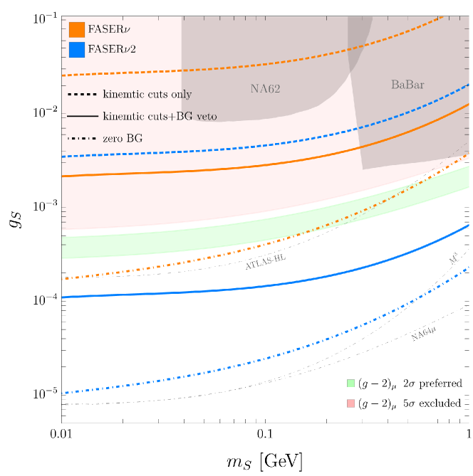
Figure 7: Projected sensitivity plot for a scalar MFC for FASER$\nu$ (orange) and FASER$\nu$2 (blue). Plotted in dahsed is the projected sensitivity using only kinematic cuts and in solid using kinematic cuts and assuming BG rejection of $5\times 10^{-5}\,(10^{-6})$ for FASER$\nu$ (FASER$\nu$2), see main text for more details. For reference, we plot the optimal sensitivity with $100$% signal efficiency and zero BG events in dot-dashed. Shaded gray region is ruled out by BaBar BaBar:2016sci ; Batell:2016ove and NA62 NA62:2021bji . The dot-dashed lines are the projected sensitivities from ATLAS-HL Galon:2019owl , M³(phase 2) Kahn:2018cqs and NA64$\mu$ ($5\times 10^{12}$ muons-on-target) Chen:2018vkr .

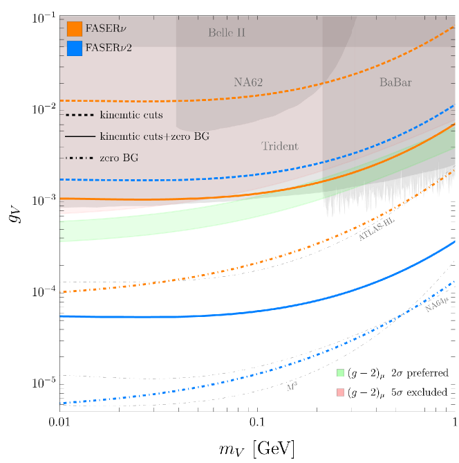
Figure 8: Projected sensitivity plot for a vector MFC for FASER$\nu$ (orange) and FASER$\nu$2 (blue). Plotted in dahsed is the projected sensitivity using only kinematic cuts and in solid using kinematic cuts and assuming BG rejection of $5\times 10^{-5}\,(10^{-6})$ for FASER$\nu$ (FASER$\nu$2), see main text for more details. For reference, we plot the optimal sensitivity with $100$% signal efficiency and zero BG events in dot-dashed. Shaded gray region is ruled out by BaBar BaBar:2016sci , NA62 NA62:2021bji , Belle II Belle-II:2019qfb and trident production CHARM-II:1990dvf ; CCFR:1991lpl ; Altmannshofer_2014 . The dot-dashed lines are the projected sensitivities from ATLAS-HL Galon:2019owl , M³ (phase 2) Kahn:2018cqs and NA64$\mu$ ($5\times 10^{12}$ muons-on-target) Gninenko:2019qiv .

5 Outlook

In this work, we propose to utilize FASER$\nu$ as a muon fixed target experiment to search for new muon force carriers (MFCs), taking advantage of the large muons flux of $\sim 10^{9}/150\,\mathrm{fb}^{-1}$. In addition to its role as a fixed target, the emulsion detector measures the muon track with excellent spatial resolution. This information can be used to measure kinks in the track, as well as the incoming and outgoing muon energies based on multiple coulomb scattering. Tracks with missing energy and large kinks are prime signatures of MFCs.

We estimate the sensitivity of the current and future runs of FASER$\nu$ to the MFC parameter space. We find that FASER$\nu$ will potentially probe previously unexplored regions of the MFC parameter space within the current run. Future runs will have substantially increased sensitivity and can be competitive with dedicated MFC searches such as M³ and NA64_μ.

This study should be considered as a proof of concept. Reaching the full potential of FASER$\nu$ would therefore require additional dedicated studies to develop and optimize various techniques, e.g. a rejection algorithm for the bremsstrahlung background events. Moreover, we did not include directional information, available due to the finite width of the emulsion layers, which can potentially improve the analysis. Another interesting possibility would be to use rare SM processes such as muon trident production in FASER$\nu$ as probe of vector MFCs.

Interestingly, a larger muon flux is expected to be found only a few meters away from the current location of FASER. A well-placed dedicated muon detector could then potentially reach sensitivities well beyond the existing bounds and future dedicated searches.

Appendix A Energy measurement analysis

We performed an analysis of the energy measurement using the MCS method at lower energies $<100\,$GeV from $\mathcal{O}(10^{3})$ simulated tracks. From each track, we used 200 shifts in both the $x$ and $y$ directions to estimate the energy of the muon using the MCS method outline in Sec. 3.1. We plot the result of our analysis in Fig. 9. We find that the absolute resolution increases at lower energies due to the larger shifts compared to the spatial resolution. The relative resolution is approximately constant at $\approx 20\,\%$, with the exception of lower energies. See Table 3 for a summary of our results.

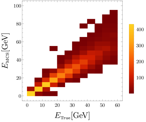
Figure 9: Density distribution of $E_{\text{MCS}}$, the measured energy using the MCS method, and the true energy $E_{\text{True}}$.

$[E_{\text{\tiny min}},E_{\text{\tiny max}}]~{}[\text{GeV}]$	# of tracks	$\langle E\rangle~{}[\text{GeV}]$	$\sigma_{E}~{}[\text{GeV}]$	$\sigma_{E}/\langle E\rangle$
[0,10]	1028	5.63	3.13	55.6 %
[10,20]	1264	15.87	4.24	26.7 %
[20,30]	1214	25.8	5.36	20.8 %
[30,40]	1060	35.76	6.84	19.1%
[40,50]	726	45.28	8.4	18.5%
[50,60]	400	56.65	10.54	18.6 %
[99.9,100.1]	3557	102.75	18.78	18.3 %

Table 3: A summary of energy measurement using the MCS method described in the text. At lower energy, larger scattering angles allow for a better (absolute) energy resolution, while the relative resolution is relatively fixed at around $20\%$ for all energies, with the exception of the first energy bin.

Appendix B Bremsstrahlung in FASER$\nu$

High-energy photons ($\gtrsim 100\,\mathrm{MeV}$) are typically converted into an $e^{+}e^{-}$ pair in the nuclear electromagnetic field. The mean free path of the photon is given by $(9/7)X_{0}$, with $X_{0}$ the radiation length of the relevant material. The physical propagation distance of a high-energy photon produced inside FASER$\nu$, which we denote by $X_{\gamma}$, is distributed according to an exponential distribution

$$\Delta_{\gamma}\sim\exp\left[-\frac{X^{\text{scat}}_{\gamma}(X_{\gamma})}{(9/7)X^{W}_{0}}\right]\,,$$ (11)

see Eq. (6) for the definition of $X^{\text{scat}}_{\gamma}(X_{\gamma})$. In addition to the propagation distance, we expect the photon angle distribution emitted from high-energy muons to be peaked around

$$\theta_{\gamma}\sim\frac{m_{\mu}}{E_{\mu}}\,.$$ (12)

This can be easily seen by examining the bremsstrahlung differential cross-section Bethe:1934za , where terms of the form ${\sin^{2}\theta}/{(E-|p|\cos\theta)^{2}}$ are maximized for $\cos\theta=\frac{p}{E}$. After taking the small-angle and high-energy limits, one recovers Eq. (12).

To validate Eqs. (11), (12), we studied $\approx 3\times 10^{5}$ simulated muon tracks associated with a hard photon emission (see Table 1) and extracted the photon information. In Fig. 10, we show the angular (left panel) and energy (right panel) distribution of the emitted photons. As expected, the angular distribution is strongly peaked around $m_{\mu}/E_{\mu}\sim 10^{-3}$, consistent with the simulated data used with a constant initial muon energy of $E_{\mu}=100\,\mathrm{GeV}$. The energy distribution is relatively flat at its bulk region, with the expected threshold at $100\,\mathrm{GeV}$ (the maximal available energy) and a tail for the low-energy photons. At shown in Fig. 5, at low energy losses, the bremsstrahlung rate is suppressed, and therefore it is not likely that a soft $\mathcal{O}(1)\,\mathrm{GeV}$ photon is responsible for the largest energy loss in a given track, which qualitatively explains the fast-dropping tail at low photon energies in Fig. 10.

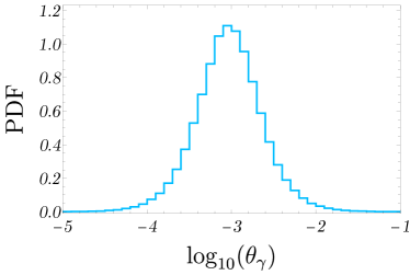
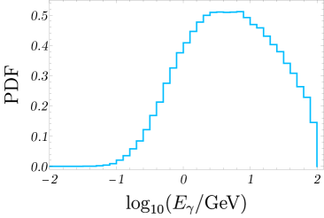
Figure 10: Left: probability distribution for the emitted photon angle $\theta_{\gamma}$. Right: probability distribution of the emitted photon energy $E_{\gamma}$.

In Fig. 11 we show the simulated distribution of $X_{\gamma}$, where we find a good agreemenet with the theoretical prediction of Eq. (11).

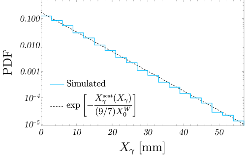
Figure 11: Probability distribution of the physical propagation distance of the photon $X_{\gamma}$ as calculated bu simulation (solid blue) compared to the analytic expectation of Eq. (11)(dashed black).

References

- (1) R. K. Ellis et al., Physics Briefing Book: Input for the European Strategy for Particle Physics Update 2020, 1910.11775.
- (2) P. Agrawal et al., Feebly-interacting particles: FIPs 2020 workshop report, Eur. Phys. J. C 81 (2021) 1015, [2102.12143].
- (3) G. Lanfranchi, M. Pospelov and P. Schuster, The Search for Feebly Interacting Particles, Ann. Rev. Nucl. Part. Sci. 71 (2021) 279–313, [2011.02157].
- (4) B. Batell, N. Lange, D. McKeen, M. Pospelov and A. Ritz, Muon anomalous magnetic moment through the leptonic Higgs portal, Phys. Rev. D 95 (2017) 075003, [1606.04943].
- (5) C.-Y. Chen, M. Pospelov and Y.-M. Zhong, Muon Beam Experiments to Probe the Dark Sector, Phys. Rev. D 95 (2017) 115005, [1701.07437].
- (6) B. Batell, A. Freitas, A. Ismail and D. Mckeen, Flavor-specific scalar mediators, Phys. Rev. D 98 (2018) 055026, [1712.10022].
- (7) L. Marsicano, M. Battaglieri, A. Celentano, R. De Vita and Y.-M. Zhong, Probing Leptophilic Dark Sectors at Electron Beam-Dump Facilities, Phys. Rev. D 98 (2018) 115022, [1812.03829].
- (8) G. W. Bennett, B. Bousquet, H. N. Brown, G. Bunce, R. M. Carey, P. Cushman et al., Final report of the e821 muon anomalous magnetic moment measurement at BNL, Physical Review D 73 (apr, 2006) .
- (9) Muon Collaboration collaboration, B. Abi, T. Albahri, S. Al-Kilani, D. Allspach, L. P. Alonzi, A. Anastasi et al., Measurement of the positive muon anomalous magnetic moment to 0.46 ppm, Phys. Rev. Lett. 126 (Apr, 2021) 141801.
- (10) M. Pospelov, Secluded U(1) below the weak scale, Phys. Rev. D 80 (2009) 095002, [0811.1030].
- (11) F. Jegerlehner and A. Nyffeler, The Muon g-2, Phys. Rept. 477 (2009) 1–110, [0902.3360].
- (12) S. Borsanyi et al., Leading hadronic contribution to the muon magnetic moment from lattice QCD, Nature 593 (2021) 51–55, [2002.12347].
- (13) C. Alexandrou et al., Lattice calculation of the short and intermediate time-distance hadronic vacuum polarization contributions to the muon magnetic moment using twisted-mass fermions, 2206.15084.
- (14) M. Cè et al., Window observable for the hadronic vacuum polarization contribution to the muon from lattice QCD, 2206.06582.
- (15) CMD-3 collaboration, F. V. Ignatov et al., Measurement of the cross section from threshold to 1.2 GeV with the CMD-3 detector, 2302.08834.
- (16) R. Balkin, C. Delaunay, M. Geller, E. Kajomovitz, G. Perez, Y. Shpilman et al., Custodial symmetry for muon g-2, Phys. Rev. D 104 (2021) 053009, [2104.08289].
- (17) BaBar collaboration, J. P. Lees et al., Search for a muonic dark force at BABAR, Phys. Rev. D 94 (2016) 011102, [1606.03501].
- (18) Belle-II collaboration, I. Adachi et al., Search for an Invisibly Decaying Boson at Belle II in Plus Missing Energy Final States, Phys. Rev. Lett. 124 (2020) 141801, [1912.11276].
- (19) G. Krnjaic, G. Marques-Tavares, D. Redigolo and K. Tobioka, Probing Muonphilic Force Carriers and Dark Matter at Kaon Factories, Phys. Rev. Lett. 124 (2020) 041802, [1902.07715].
- (20) NA62 collaboration, E. Cortina Gil et al., Search for decays to a muon and invisible particles, Phys. Lett. B 816 (2021) 136259, [2101.12304].
- (21) CHARM-II collaboration, D. Geiregat et al., First observation of neutrino trident production, Phys. Lett. B 245 (1990) 271–275.
- (22) CCFR collaboration, S. R. Mishra et al., Neutrino tridents and W Z interference, Phys. Rev. Lett. 66 (1991) 3117–3120.
- (23) W. Altmannshofer, S. Gori, M. Pospelov and I. Yavin, Neutrino trident production: A powerful probe of new physics with neutrino beams, Physical Review Letters 113 (aug, 2014) .
- (24) D. Croon, G. Elor, R. K. Leane and S. D. McDermott, Supernova Muons: New Constraints on ’ Bosons, Axions and ALPs, JHEP 01 (2021) 107, [2006.13942].
- (25) C.-Y. Chen, J. Kozaczuk and Y.-M. Zhong, Exploring leptophilic dark matter with NA64-, JHEP 10 (2018) 154, [1807.03790].
- (26) S. N. Gninenko, D. V. Kirpichnikov, M. M. Kirsanov and N. V. Krasnikov, Combined search for light dark matter with electron and muon beams at NA64, Phys. Lett. B 796 (2019) 117–122, [1903.07899].
- (27) Y. Kahn, G. Krnjaic, N. Tran and A. Whitbeck, M3: a new muon missing momentum experiment to probe (g 2)μ and dark matter at Fermilab, JHEP 09 (2018) 153, [1804.03144].
- (28) D. Forbes, C. Herwig, Y. Kahn, G. Krnjaic, C. Mantilla Suarez, N. Tran et al., New Searches for Muonphilic Particles at Proton Beam Dump Spectrometers, 2212.00033.
- (29) I. Galon, E. Kajamovitz, D. Shih, Y. Soreq and S. Tarem, Searching for muonic forces with the ATLAS detector, Phys. Rev. D 101 (2020) 011701, [1906.09272].
- (30) FASER collaboration, H. Abreu et al., Detecting and Studying High-Energy Collider Neutrinos with FASER at the LHC, Eur. Phys. J. C 80 (2020) 61, [1908.02310].
- (31) FASER collaboration, H. Abreu et al., Technical Proposal: FASERnu, 2001.03073.
- (32) FASER collaboration, H. Abreu et al., First neutrino interaction candidates at the LHC, Phys. Rev. D 104 (2021) L091101, [2105.06197].
- (33) J. L. Feng, I. Galon, F. Kling and S. Trojanowski, ForwArd search ExpeRiment at the LHC, Physical Review D 97 (feb, 2018) .
- (34) FASER collaboration, A. Ariga et al., Letter of Intent for FASER: ForwArd Search ExpeRiment at the LHC, 1811.10243.
- (35) FASER collaboration, A. Ariga et al., Technical Proposal for FASER: ForwArd Search ExpeRiment at the LHC, 1812.09139.
- (36) FASER collaboration, A. Ariga et al., FASER’s physics reach for long-lived particles, Phys. Rev. D 99 (2019) 095011, [1811.12522].
- (37) X. G. He, G. C. Joshi, H. Lew and R. R. Volkas, NEW Z-prime PHENOMENOLOGY, Phys. Rev. D 43 (1991) 22–24.
- (38) R. Foot, New Physics From Electric Charge Quantization?, Mod. Phys. Lett. A 6 (1991) 527–530.
- (39) X.-G. He, G. C. Joshi, H. Lew and R. R. Volkas, Simplest model, Phys. Rev. D 44 (Oct, 1991) 2118–2132.
- (40) FASER collaboration, H. Abreu et al., First Direct Observation of Collider Neutrinos with FASER at the LHC, 2303.14185.
- (41) K. Kodama et al., Detection and analysis of tau neutrino interactions in DONUT emulsion target, Nucl. Instrum. Meth. A 493 (2002) 45–66.
- (42) OPERA collaboration, N. Agafonova et al., Momentum measurement by the Multiple Coulomb Scattering method in the OPERA lead emulsion target, New J. Phys. 14 (2012) 013026, [1106.6211].
- (43) H. A. Bethe, Moliere’s theory of multiple scattering, Phys. Rev. 89 (1953) 1256–1266.
- (44) W. T. Scott, The theory of small-angle multiple scattering of fast charged particles, Rev. Mod. Phys. 35 (1963) 231–313.
- (45) J. W. MOTZ, H. OLSEN and H. W. KOCH, Electron Scattering without Atomic or Nuclear Excitation, Rev. Mod. Phys. 36 (1964) 881–928.
- (46) G. R. Lynch and O. I. Dahl, Approximations to multiple Coulomb scattering, Nucl. Instrum. Meth. B 58 (1991) 6–10.
- (47) Particle Data Group collaboration, R. L. Workman and Others, Review of Particle Physics, PTEP 2022 (2022) 083C01.
- (48) H. Kawahara, Fasernu: Current status and first data from lhc run 3, http://indico.cern.ch/event/1166678/contributions/5082108/ (October, 2022) .
- (49) J. Alwall, R. Frederix, S. Frixione, V. Hirschi, F. Maltoni, O. Mattelaer et al., The automated computation of tree-level and next-to-leading order differential cross sections, and their matching to parton shower simulations, JHEP 07 (2014) 079, [1405.0301].
- (50) GEANT4 collaboration, S. Agostinelli et al., GEANT4–a simulation toolkit, Nucl. Instrum. Meth. A 506 (2003) 250–303.
- (51) A. G. Bogdanov, H. Burkhardt, V. N. Ivanchenko, S. R. Kelner, R. P. Kokoulin, M. Maire et al., Geant4 simulation of production and interaction of muons, IEEE Trans. Nucl. Sci. 53 (2006) 513–519.
- (52) J. L. Feng et al., The Forward Physics Facility at the High-Luminosity LHC, J. Phys. G 50 (2023) 030501, [2203.05090].
- (53) H. Bethe and W. Heitler, On the Stopping of fast particles and on the creation of positive electrons, Proc. Roy. Soc. Lond. A 146 (1934) 83–112.