Convergence to Lexicographically Optimal Base in a (Contra)Polymatroid and Applications to Densest Subgraph and Tree Packing

Abstract

Boob et al. [1] described an iterative peeling algorithm called Greedy++ for the Densest Subgraph Problem (DSG) and conjectured that it converges to an optimum solution. Chekuri, Qaunrud and Torres [2] extended the algorithm to general supermodular density problems (of which DSG is a special case) and proved that the resulting algorithm Super-Greedy++ (and hence also Greedy++) converges. In this paper we revisit the convergence proof and provide a different perspective. This is done via a connection to Fujishige’s quadratic program for finding a lexicographically optimal base in a (contra) polymatroid [3], and a noisy version of the Frank-Wolfe method from convex optimization [4, 5]. This gives us a simpler convergence proof, and also shows a stronger property that Super-Greedy++ converges to the optimal dense decomposition vector, answering a question raised in Harb et al. [6]. A second contribution of the paper is to understand Thorup’s work on ideal tree packing and greedy tree packing [7, 8] via the Frank-Wolfe algorithm applied to find a lexicographically optimum base in the graphic matroid. This yields a simpler and transparent proof. The two results appear disparate but are unified via Fujishige’s result and convex optimization.

1 Introduction

In this paper we consider iterative greedy algorithms for two different combinatorial optimization problems and show that the convergence of these algorithms can be understood by combining two general tools, one coming from the theory of submodular functions, and the other coming from convex optimization. This yields simpler proofs via a unified perspective, while also yielding additional properties that were previously unknown.

Densest subgraph and supermodularity: We start with the initial problem that motivated this work, namely, the densest subgraph problem (DSG). The input to DSG is an undirected graph $G=(V,E)$ with $m=\left|{E}\right|$ and $n=\left|{V}\right|$. The goal is to return a subset $S\subseteq V$ that maximizes $\frac{\left|{E(S)}\right|}{\left|{S}\right|}$ where $E(S)=\{uv\in E:u,v\in S\}$ is the set of edges with both end points in $S$. Throughout the paper, we let $\lambda(G)=\frac{\left|{E(G)}\right|}{\left|{V(G)}\right|}$ denote the density of graph $G(V,E)$. We treat the unweighted case for simplicity; all the results generalize to edge-weighted graphs. Goldberg [9] and Picard and Queyranne [10] showed that DSG can be efficiently solved via a reduction to the $s$-$t$ maximum-flow problem.

A different connection that shows polynomial-time solvability of DSG is important to this paper. Consider a real-valued set function $f:2^{V}\rightarrow\mathbb{R}_{+}$ defined over the vertex set $V$, where $f(S)=|E(S)|$. This function is supermodular. A function $f$ is supermodular iff $-f$ is submodular. A real-valued set function $f:2^{V}\rightarrow\mathbb{R}$ is submodular iff $f(A)+f(B)\geq f(A\cup B)+f(A\cap B)$ for all $A,B\subseteq B$. Submodular and supermodular set functions are fundamental in combinatorial optimization — see [11, 12].

Coming back to DSG, maximizing $|E(S)|/|S|$ is equivalent to finding the largest $\lambda$ such that $\lambda|S|-|E(S)|\geq 0$ for all $S\subseteq V$. This corresponds to minimizing the submodular function $g$ where $g(S)=\lambda|S|-|E(S)|$. A classical result in combinatorial optimization is that the minimum of a submodular set function can be found in polynomial-time in the value oracle setting. Thus, DSG can be solved via reduction to submodular set function minimization and binary search. The preceding connection also motivates the definition of a generalization of DSG called the densest supermodular set problem (DSS) (see [2]). The input is a non-negative supermodular function $f:2^{V}\rightarrow\Re_{+}$, and the goal is to find $S\subseteq V$ that maximizes $\frac{f(S)}{|S|}$. DSS is polynomial-time solvable via submodular set function minimization. DSG, DSS and its variants have several applications in practice, and they are routinely used in graph and network analysis to find dense clusters or communities. We refer the reader to the extensive literature on this topic [13, 1, 14, 15, 16, 17, 18, 19, 20, 21, 22, 23, 24, 25, 26, 27]. DSG is also of interest in algorithms via its connection to arboricity and related notions — see [28, 29] for recent work.

Faster algorithms, Greedy and Greedy++: Although DSG is polynomial-time solvable via maxflow and submodular function minimization, the corresponding algorithms are not yet practical for the large graphs that arise in many applications; this is despite the fact that we now have very fast theoretical algorithms for maxflow and mincost flow [30]. For this reason there has been considerable interest in faster (approximation) algorithms. More than 20 years ago Charikar [31] showed that a simple “peeling” algorithm (Greedy) yields a $1/2$-approximation for DSG. An ordering of the vertices as $v_{i_{1}},v_{i_{2}},\ldots,v_{i_{n}}$ is computed as follows: $v_{i_{1}}$ is a vertex of minimum degree in $G$ (ties broken arbitrarily), $v_{i_{2}}$ is a minimum degree vertex in $G-v_{i_{1}}$ and so on. After creating the ordering, the algorithm picks the best suffix, in terms of density, among the $n$-possible suffixes of the ordering. Charikar also developed a simple exact LP relaxation for DSG. Charikar’s results have been quite influential. Greedy can be implemented in (near)-linear time and has also been adapted to other variants. The LP relaxation has also been used in several algorithms that yield a $(1-\epsilon)$-approximate solution [34, 35], and has led to a flow-based $(1-\epsilon)$-approximation [2]. More recently, Boob et al. [1] developed an algorithm called Greedy++ that is based on combining Greedy with ideas from multiplicative weight updates (MWU); the algorithm repeatedly applies a simple peeling algorithm with the first iteration coinciding with Greedy but later iterations depending on a weight vector that is maintained on the vertices — the formal algorithm is described in a later section. The advantage of the algorithm is its simplicity, and Boob et al. [1] showed that it has very good empirical performance. Moreover they conjectured that Greedy++ converges to a $(1-\epsilon)$-approximation in $O(1/\epsilon^{2})$ iterations. Although their strong conjecture is yet unverified, Chekuri et al. [2] proved that Greedy++ converges in $O(\frac{\Delta\log|V|}{\epsilon^{2}\lambda(G)})$ iterations where $\Delta$ is the maximum degree of $G$.

The convergence proof in [2] is non-trivial. The proof relies crucially in considering DSS and supermodularity. [2] shows that Greedy and Greedy++ can be generalized to SuperGreedy and SuperGreedy++ for DSS, and that SuperGreedy++ converges to a $(1-\epsilon)$-approximation solution in $O(\alpha_{f}/\epsilon^{2})$ iterations where $\alpha_{f}$ depends (only) on the function $f$.

Dense subgraph decomposition and connections: As we discussed, DSG is a special case of DSS and hence DSG inherits certain nice structural properties from supermodularity. One of these is the fact that the vertex set $V$ of every graph $G=(V,E)$ admits a decomposition into $S_{1},S_{2},\ldots,S_{k}$ for some $k$ where $S_{1}$ is the vertex set of the unique maximal densest subgraph, $S_{2}$ is the unique maximal densest subgraph after “contracting” $S_{1}$, and so on. This fact is easier to see in the setting of DSS. Here, the fact that $S_{1}$ is the unique maximal densest set and this follows from supermodularity; if $A$ and $B$ are optimum dense sets then so is $A\cup B$. One can then consider a new supermodular function $f_{S_{1}}:2^{V-S_{1}}\rightarrow\mathbb{R}$ defined over $V-S_{1}$ where $f_{S_{1}}(A)=f(S_{1}\cup A)-f(S_{1})$ for all $A\subseteq V-S_{1}$. The new function is also supermodular. Then $S_{2}$ is the unique maximal densest set for $f_{S_{1}}$. We iterate this process until we obtain an empty set. The decomposition also allows us to assign a density value $\lambda_{v}$ to each $v\in V$ (which corresponds to the density of the set when $v$ is in the maximal set). We call this the density vector associated with $f$. Dense decompositions follow from the theory of principal partitions of submodular functions [36, 37, 38]. In the context of graphs and DSG this was rediscovered by Tatti and Gionis who called it the locally-dense decomposition [39, 40], and gave algorithms for computing it. Subsequently, Danisch et al.[14] applied the well-known Frank-Wolfe algorithm for constrained convex optimization to a quadratic program derived from Charikar’s LP relaxation for DSG. More recently, Harb et al. [6] obtained faster algorithms for computing the dense decomposition in graphs via Charikar’s LP; they used a different method called FISTA for constrained convex optimization based on acceleration. Although DSS was not the main focus, [6] also made an important connection to Fujishige’s result on lexicographically optimal base in polymatroids [3] which elucidated the work of Danisch et al. on DSG. We describe this next.

Lexicographical optimal base and dense decomposition: We briefly describe Fujishige’s result [3] and its connection to dense decompositions. Let $f:2^{V}\rightarrow\mathbb{R}_{+}$ be a monotone submodular set function ($f(A)\leq f(B)$ if $A\subset B$) that is also normalized ($f(\emptyset)=0$). Following Edmonds, the polymatroid associated with $f$, denote by $P_{f}$ is the polyhedron $\{x\in\mathbb{R}^{V}\mid x\geq 0,x(S)\leq f(S)\quad\forall S\subseteq V\},$ where $x(S)=\sum_{i\in S}x_{i}$. The base polyhedron associated with $f$, denote by $B_{f}=P_{f}\cap\{x\in\mathbb{R}^{V}\mid x(V)=f(V)\}$ obtained by intersecting $P_{f}$ with the equality constraint $x(V)=f(V)$. Each vector $x$ in $B_{f}$ is called a base. If $f$ is a monotone normalized supermodular function we consider the contrapolymatroid $P_{f}=\{x\in\mathbb{R}^{V}\mid x\geq 0,x(S)\geq f(S)\quad\forall S\subseteq V\}$ (the inequalities are reversed), and similarly $B_{f}$ is the base contrapolymatroid obtained by intersecting $P_{f}$ with equality constraint $x(V)=f(V)$. Fujishige proved that there exists a unique lexicographically minimal base in any polymatroid, and morover it can found by solving the quadratic program: $\min\sum_{v}x_{v}^{2}\mbox{\leavevmode\nobreak\ s.t\leavevmode\nobreak\ }x\in B_{f}$. In the context of supermodular functions, one obtains a similar result; the quadratic program $\min\sum_{v}x_{v}^{2}\mbox{\leavevmode\nobreak\ s.t\leavevmode\nobreak\ }x\in B_{f}$ where $B_{f}$ is contrapolymatroid associated with $f$ has a unique solution. As observed explicity in [6], the lexicographically optimal base gives the dense decomposition vector for DSS. That is, if $x^{*}$ is the optimal solution to the quadratic program then for each $v$, $x^{*}_{v}=\lambda_{v}$. In particular, as noted in [6], one can apply the well-known Frank-Wolfe algorithm to the quadratic program and it converges to the dense decomposition vector. As we will see later, each iteration corresponds to finding a maximum weight base in a contrapolymatroid which is easy to find via the greedy algorithm.

(Ideal) Tree packings in graphs and the Tutte–Nash-Williams theorem: Our discussion so far focused on DSG. Now we describe a different problem on graphs and relevant background. As we said, our goal is to present a unified perspective on these two problems. The well-known Tutte–Nash-Williams theorem in graph theory (see [11]) establishes a min-max result for the maximum number of edge-disjoint spanning trees in a multi-graph $G$. Given an undirected graph $G=(V,E)$, and a partition $P$ of the vertices, let $E(P)$ denote the number of edges crossing from one partition to another. We say the strength of a partition is $\frac{E(P)}{|P|-1}$. Let $\mathcal{T}(G)$ denote all possible spanning trees of $G$. Let $\tau^{*}(G)$ denote the maximum number of edge-disjoint spanning trees in $G$. Then $\tau^{*}(G)=\min_{P}\lfloor\frac{E(P)}{|P|-1}\rfloor$. Further, if we define $\tau(G)$ to be the maximum fractional packing of spanning trees, then the floor can be removed and we have $\tau(G)=\min_{P}\frac{E(P)}{|P|-1}$. We note that the graph theoretic result is a special case of matroid base packing. Tree packings are useful for a number of applications. In particular, Karger [41] used tree packings and other ideas in his well-known near-linear randomized algorithm for computing the global minimum cut of a graph. We are mainly concerned here with Thorup’s work in [7, 8] that was motivated by dynamic mincut and $k$-cut problems. He defined the so-called ideal edge loads and ideal tree packing (details in later section) by recursively decomposing the graph via Tutte–Nash-Williams partitions [7]. He also proved that a simple iterative greedy tree packing algorithm converges to the ideal loads [8]. He used the approximate ideal tree packing to obtain new deterministic algorithms for the $k$-cut problem, and his approach has been quite influential in a number of subsequent results [42, 43, 44, 45, 46]. Thorup obtained his tree packing result from first principles. We ask: is there a connection between ideal tree packing and DSG?

1.1 Contributions of the paper

This paper has two main contributions. The first is a new proof of the convergence of SuperGreedy++ for DSS. Our proof is based on showing that SuperGreedy++ can be viewed as a “noisy” or “approximate” variant of the Frank-Wolfe algorithm applied to the quadratic program defined by Fujishige. The advantage of the new proof is twofold. First, it shows that SuperGreedy++ not only converges to a $(1-\epsilon)$-approximation to the densest set, but that in fact it converges to the densest decomposition vector. This was empirically observed in [6] for DSG, and was left as an open problem to resolve. The proof in [2] on convergence of SuperGreedy++ is based on the MWU method via LPs, and does not exploit Fujishige’s result which is key to the stronger property that we prove here. Second, the proof connects two powerful tools directly and at a high-level: Fujishige’s result on submodular functions, and a standard method for constrained convex optimization.

Theorem 1.1.

Let $b^{*}$ be the dense decomposition vector for a non-negative monotone supermodular set function $f:2^{V}\rightarrow\mathbb{R}_{+}$ where $|V|=n$. Then, SuperGreedy++ converges in $O(\alpha_{f}/\epsilon^{2})$ iterations to a vector $b$ such that $||b-b^{*}||_{2}\leq\epsilon$, where $\alpha_{f}$ depends only on $f$. For a graph with $m$ edges and $n$ vertices, Greedy++ converges in $O(mn^{2}/\epsilon^{2})$ iterations for unweighted multigraphs.

Remark 1.2.

The new convergence gives a weaker bound than the one in [2] in terms of convergence to a $(1-\epsilon)$ relative approximation to the maximum density. However, it gives a strong additive guarantee to the entire dense decomposition vector.

Our second contribution builds on our insights on DSG and DSS, and applies it towards understanding ideal tree packing and greed tree packing. We connect the ideal tree packing of Thorup to the dense decomposition associated with the rank function of the underlying graphic matroid (which is submodular). We then show that greedy tree packing algorithm can be viewed as the Frank-Wolfe algorithm applied to the quadratic program defined by Fujishige, and this easily yields a convergence guarantee.

Theorem 1.3.

Let $G=(V,E)$ be a graph. The ideal edge load vector $\ell^{*}:E\rightarrow\mathbb{R}_{+}$ for $G$ is given by the lexicographically minimal base in the polymatroid associated with the rank function of the graphic matroid of $G$. The Frank-Wolfe algorithm with step size $\frac{1}{k+1}$, when applied to the quadratic program for computing the lexicographically minimal base in the graphic matroid of $G$, coincides with the greedy tree packing algorithm. For unweighted graphs on $m$ edges, the generic analysis of Frank-Wolfe method’s convergence shows that greedy tree packing converges to a load vector $\ell:E\rightarrow\mathbb{R}_{+}$ such that $||\ell-\ell^{*}||\leq\epsilon$ in $O(\frac{m\log(m/\epsilon)}{\epsilon^{2}})$ iterations. The standard step size algorithm converges in $O(\frac{m}{\epsilon^{2}})$ iterations.

Remark 1.4.

Although the algorithm is the same (greedy tree packing), Thorup’s analysis guarantees a strongly polynomial-bound even in the capacitated case [8]. However we obtain a stronger additive guarantee via a generic Frank-Wolfe analysis and our analysis has a $1/\epsilon^{2}$ dependence while Thorup’s has a $1/\epsilon^{3}$ dependence. We give a more detailed comparison in Section 5.

Organization: The rest of the paper is devoted to proving the two theorems. The paper relies on tools from theory of submodular functions and an adaptation of the analysis of Frank-Wolfe method. We first describe the relevant background and then prove the two results in separate sections. Due to space constraints, most of the proofs are provided in the appendix. A future version will discuss additional related work in more detail.

2 Background on Frank-Wolfe algorithm and a variation

Let $\mathcal{D}\subseteq\Re^{d}$ be a compact convex set, and $f:\mathcal{D}\rightarrow\Re$ be a convex, differentiable function. Consider the problem of $\min_{x\in\mathcal{D}}f(x)$. Frank-Wolfe method [4] is a first order method and it relies on access to a linear minimization oracle, LMO, for $f$ that can answer $\textsc{LMO}(w)=\operatorname*{arg\,min}\limits_{s\in\mathcal{D}}\langle s,\nabla f(w)\rangle$ for any given $w\in\mathcal{D}$. In several applications such oracles with fast running times exist. Given $f,\mathcal{D}$ as above, the Frank-Wolfe algorithm is an iterative algorithm that converges to the minimizer ${\bf x}^{\ast}\in\mathcal{D}$ of $f$. See Algorithm 1. The algorithm starts with a guess of the minimizer $b^{(0)}\in\mathcal{D}$. In each iteration, it finds a direction $d^{(k+1)}$ to move towards by calling the linear minimization oracle on the current guess $b^{(k)}$. It then moves slightly towards that direction using a convex combination to ensure that the new point is in $\mathcal{D}$. The amount the algorithm moves towards the new direction decreases as $k$ increases signifying the “confidence” in its current guess as the minimizer.

1:Initialize $b^{(0)}\in\mathcal{D}$

2:for $k\leftarrow 0$ to $T-1$ do

3:     $\gamma\leftarrow\frac{2}{k+2}$

4:     $d^{(k+1)}\leftarrow\operatorname*{arg\,min}\limits_{s\in\mathcal{D}}(\langle s,\nabla f(b^{(k)})\rangle)$ $\triangleright$ Call oracle on $b^{(k)}$

5:     $b^{(k+1)}\leftarrow(1-\gamma)b^{(k)}+\gamma d^{(k+1)}$ return $b^{(T)}$

Algorithm 1 Frank-Wolfe-Original

The original convergence analysis for the Frank-Wolfe algorithm is from [4]. Jaggi [5] gave an elegant and simpler analysis. His analysis characterizes the convergence rate in terms of the curvature constant $C_{f}$ of the function $f$.

Definition 2.1.

Let $\mathcal{D}\subseteq\Re^{d}$ be a compact convex set, and $f:\mathcal{D}\rightarrow\Re$ be a convex, differentiable function. The curvature constant $C_{f}$ of $f$ is defined as

$$C_{f}=\sup_{x,s\in D,\gamma\in[0,1],y=x+\gamma(s-x)}\frac{2}{\gamma^{2}}(f(y)-f(x)-\langle y-x,\nabla f(x)\rangle).$$

Definition 2.2.

Let $g:\mathcal{D}\rightarrow\Re$ be a differentiable function. Then $g$ is Lipschitz with constant $L$ if for all $x,y\in\mathcal{D}$, $\left\|g({\bf x})-g({\bf y})\right\|_{2}\leq L\left\|x-y\right\|_{2}$.

Let $\text{diam}(\mathcal{D})=\max\limits_{x,y\in\mathcal{D}}\left\|x-y\right\|_{2}$ be the diameter of $\mathcal{D}$. One can show that $C_{f}\leq L\cdot\text{diam}(\mathcal{D})^{2}$ where $L$ is the Lpischitz constant of $\nabla f$.

Theorem 2.3 ([5]).

Let $\mathcal{D}\subseteq\Re^{d}$ be a compact convex set, and $f:\mathcal{D}\rightarrow\Re$ be a convex, differentiable function with minimizer ${\bf b}^{\ast}$. Let ${\bf b}^{(k)}$ denote the guess on the $k$-th iteration of the Frank-Wolfe algorithm. Then $f({\bf b}^{(k)})-f({\bf b}^{\ast})\leq\frac{2C_{f}}{k+2}$.

Jaggi’s proof technique can be used to prove the convergence rate of “noisy/approximate” variants of the Frank-Wolfe algorithm. This motivates the following definition. An $\epsilon$-approximate linear minimization oracle is an oracle that for any ${\bf w}\in\mathcal{D}$, returns $\hat{{\bf s}}$ such that $\langle{\hat{\bf s}},\nabla f({\bf w})\rangle\leq\langle{\bf s}^{\ast},\nabla f({\bf w})\rangle+\epsilon$, where $s^{\ast}=\textsc{LMO}({\bf w})$. While an efficient exact linear minimization oracle exists in some applications, in others one can only $\epsilon$-approximate it (using numerical methods or otherwise). Jaggi’s proof technique extends to show that an approximate linear minimization oracles suffices for convergence as long as the approximation quality improves with the iterations. Suppose the oracle, in iteration $k$, provides a $\frac{\delta C_{f}}{k+2}$-approximate solution where $\delta>0$ is some fixed constant. The convergence rate will only deteriorate by a $(1+\delta)$ multiplicative factor. Qualitatively, this says that we can afford to be inaccurate in computing the Frank-Wolfe direction in early iterations, but the approximation should approach $\textsc{LMO}(b^{(k)})$ as $k\rightarrow\infty$.

Another question of interest is the resilience of the Frank-Wolfe algorithm to changes in the learning rate $\gamma_{k}=\frac{2}{k+2}$. Indeed, the variants we will look at will require $\gamma_{k}=\frac{1}{k+1}$. As we will see, Jaggi’s proof can again be adapted to handle this case, with only an $O(\log k)$ multiplicative deterioration in the convergence rate. We state the following theorem whose proof we defer to the appendix.

Theorem 2.4.

[Proof in Appendix 7.1] Let $\mathcal{D}\subseteq\Re^{d}$ be a compact convex set, and $f:\mathcal{D}\rightarrow\Re$ be a convex, differentiable function with minimizer ${\bf b}^{\ast}$. Suppose instead of computing ${\bf d}^{(k+1)}$ by calling $\textsc{LMO}({\bf b^{(k)}})$ in iteration $k$, we call a $\frac{\delta C_{f}}{k+2}$-approximate linear minimization oracle, for some fixed $\delta>0$. Also, suppose instead of using $\gamma_{k}=\frac{2}{k+2}$, we use $\gamma_{k}=\frac{1}{k+1}$ as a step size. Then $f({\bf b}^{(k)})-f({\bf b}^{\ast})\leq\frac{2C_{f}(1+\delta)H_{k+1}}{k+1}$, where $H_{n}$ is the $n$-th Harmonic term.

We refer to the variant of Frank-Wolfe algorithm as described by Theorem 2.4 as noisy Frank-Wolfe.

3 Sub and supermodular functions, and dense decompositions

We already defined submodular and supermodular set functions, polymatroids and contrapolymatroids. We restrict attention to functions satisfying $f(\emptyset)=0$ which together with supermodularity and non-negativity implies monotonocity, that is, $f(A)\leq f(B)$ for $A\subseteq B$. An alternative definition of submodularity is via diminishing marginal values. We let $f(v\mid A)=f(A\cup\{v\})-f(A)$ denote the marginal value of $v$ to $A$. Submodularity is equivalent to $f(v\mid A)\geq f(v\mid B)$ whenever $A\subseteq B$ and $v\in V\setminus B$; the inequality is reversed for supermodular set functions. We need the following simple lemma.

Lemma 3.1.

[Proof in Appendix 7.2] For a submodular function $f:2^{V}\rightarrow\Re$, the function $g(X)=f(V)-f(V\setminus X)$ is supermodular. In particular if $f$ is a normalized monotone submodular function then $g$ is a normalized monotone supermodular function.

Deletion and contraction, and non-negative summation: Sub and supermodular functions are closed under a few simple operations. Given $f:2^{V}\rightarrow\mathbb{R}$, restricting it to a subset $V^{\prime}$ corresponds to deleting $V\setminus V^{\prime}$. Given $A\subset V$, contracting $f$ to $A$ yields the function $g:2^{V\setminus A}\rightarrow\mathbb{R}$ where $g(X)=g(X\cup A)-g(A)$. Given two functions $f$ and $g$ we can take their non-negative sum $af+bg$ where $a,b\geq 0$. Monotonicity and normalization is also preserved under these operations.

3.1 Dense decompositions for submodular and supermodular functions

Following the discussion in the introduction, we are interested in decompositions of supermodular and submodular functions. Dense decompositions follow from the theory of principal partitions of submodular functions that have been explored extensively. We refer the reader to Fujishige’s survey [38] as well as Naraynan’s work [36, 37]. The standard perspective comes from considering the minimizers of the function $f_{\lambda}$ for a scalar $\lambda$ where $f_{\lambda}(S)-\lambda|S|$. As $\lambda$ varies from $-\infty$ to $\infty$ the minimizers change only at a finite number of break points. In this paper we are interested in the notion of density, in the form of ratios, for non-negative submodular and supermodular functions. For this reason we follow the notation from recent work [40, 14, 2, 6] and state lemmas in a convenient form, and provide proofs in the appendix for the sake of completeness.

Supermodular function dense decomposition: The basic observation is the following.

Lemma 3.2.

[Proof in Appendix 7.3] Let $f:2^{V}\rightarrow\Re_{+}$ be a non-negative supermodular set function. There exists a unique maximal set $S\subseteq V$ that maximizes $\frac{f(S)}{\left|{S}\right|}$.

The preceding lemma can be used in a simple fashion to derive the following corollary (this was explicitly noted in [2] for instance).

Corollary 3.3.

Let $f:2^{V}\rightarrow\Re_{+}$ be a non-negative supermodular set function. There is a unique partition $S_{1},S_{2},\ldots,S_{h}$ of $V$ with the following property. Let $V_{i}=V-\cup_{j<i}S_{j}$ and let $A_{i}=\cup_{j<i}S_{i}$. Then, for each $i=1$ to $h$, $S_{i}$ is the unique maximal densest set for the function $f_{D_{i}}:2^{V_{i}}\rightarrow\mathbb{R}_{+}$. Moroever, letting $\lambda_{i}$ be the optimum density of $f_{D_{i}}$, we have $\lambda_{1}>\lambda_{2}\ldots>\lambda_{h}$.

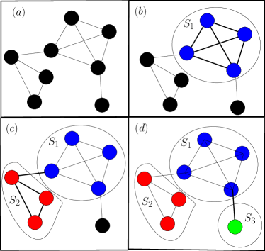
Figure 1: Densest Subgraph Decomposition Example. The densest subgraph $S_{1}$ is shown in $(b)$ with blue vertices with density $6/4=1.5$. We “contract” $S_{1}$ (the blue vertices) and find the densest subgraph $S_{2}$ with density $(3+1)/3=4/3$. Finally, we contract $S_{2}$, and find $S_{3}$ with density $(0+1)/1=1$.

Based on the preceding corollary, we can associated with each $v\in V$ a value $\lambda(v)$: $\lambda(v)=\lambda_{i}$ where $v\in S_{i}$. See Figure 1 for an example of a dense decomposition of the function $f(S)=\left|{E(S)}\right|$.

Dense decomposition for submodular functions: We now discuss submodular functions. We consider two variants. We start with a basic observation.

Lemma 3.4.

[Proof in Appendix 7.4] Let $f:2^{V}\rightarrow\Re_{+}$ be a monotone non-negative submodular set function such that $f(v)>0$ for all $v\in V$. There is a unique minimal set $S\subseteq V$ that minimizes $\frac{\left|{V}\right|-\left|{S}\right|}{f(V)-f(S)}$ for submodular function $f$.

Consider the following variant of a decomposition of $f$. We let $S_{0}=V$ and find $S_{1}$ as the unique minimal set $S\subseteq V$ that minimizes $\frac{|V|-|S|}{f(V)-f(S)}$. Then we “delete” $\hat{S_{1}}=V\setminus S_{1}$, and find the minimal set $S_{2}\subseteq S_{1}$ that minimizes $\frac{|S_{1}|-|S|}{f(S_{1})-f(S)}$. In iteration $i$, we find the unique minimal set $S_{i}\subset S_{i-1}$ that minimizes $\frac{|S_{i-1}|-|S_{i}|}{f(S_{i-1})-f(S_{i})}$. Notice that $S_{k}\subset S_{k-1}\subset...\subset S_{1}\subset V$. We say the relative density of $\hat{S_{i}}=S_{i-1}\setminus S_{i}$ is $\lambda_{i}=\frac{|S_{i-1}|-|S_{i}|}{f(S_{i-1})-f(S_{i})}$. For $u\in\hat{S}_{i}$, we say the density of $u$ is $\lambda_{u}=\lambda_{i}$. Hence the dense decomposition of $f$ is $\hat{S}_{1},...,\hat{S}_{k}$ with densities $\lambda_{1},\ldots,\lambda_{k}$. We refer to this decomposition as the first variant which is based on deletions.

We now describe a second dense decomposition for submodular functions. Let $f:2^{V}\rightarrow\mathbb{R}_{+}$ be a monotone submodular function. Consider the supermodular function $g:2^{V}\rightarrow\mathbb{R}_{+}$ where $g(X)=f(V)-f(V\setminus X)$ for all $X\subseteq V$. From Lemma 3.1, $g$ is monotone supermodular. We can then apply Corollary 3.3 to obtain a dense decomposition of $g$. Let $T_{1},T_{2},\ldots,T_{k^{\prime}}$ be the unique decomposition obtained by considering $g$ and let $\hat{\lambda}_{1},...,\hat{\lambda}_{k^{\prime}}$ be the corresponding densities. Note that this second decomposition is based on contractions.

Not too surprisingly, the two decompositions coincide, as we show in the next theorem. The main reason to consider them separately is for technical ease in applications where one or the other view is more natural.

Theorem 3.5.

[Proof of Appendix 7.5] Let $\hat{S}_{1},...,\hat{S}_{k}$ be a dense decomposition (using deletion variant) of a submodular function $f$ with densities $\lambda_{i},\ldots,\lambda_{k}$. Let $T_{1},...,T_{k^{\prime}}$ be a dense decomposition (using contraction variant) of the same function with densities $\hat{\lambda}_{1},...,\hat{\lambda}_{k^{\prime}}$. We have (i) $k^{\prime}=k$, (ii) $\hat{S}_{1},...\hat{S}_{k}$ is exactly $T_{1},...,T_{k}$, and (iii) $\hat{\lambda}_{i}=\frac{1}{\lambda_{i}}$ for $1\leq i\leq k$.

3.2 Fujishige’s results on lexicographically optimal bases

Fujishige [3] gave a polyhedral view of the dense decomposition which is the central ingredient in our work. He stated his theorem for polymatroids, however, it can be easily generalized to contrapolymatroids. We restrict attention to the unweighted case for notational ease — [3] treats the weighted case.

Vectors in $\mathbb{R}^{n}$ can be totally ordered by sorting the coordinates in increasing order and considering the lexicographical ordering of the two sorted sequences of length $n$. In the following, for $a,b\in\mathbb{R}^{n}$ we use $a\prec b$ and $a\preceq b$ to refer to this order. We say that a vector $x$ in a set $D$ is lexicographically minimum (maximum) if for all $y\in D$ we have $x\preceq y$ ($y\preceq x$).

Fujishige proved the following theorem for polymatroids.

Theorem 3.6 ([3]).

Let $f:2^{V}\rightarrow\mathbb{R}_{+}$ be a monotone submodular function (a polymatroid) and let $B_{f}$ be its base polytope. Then there is a unique lexicographically maximum base $b^{*}\in B_{f}$ and for each $v\in V$, $b^{*}_{v}=\lambda_{v}$. Moroever, $b^{*}$ is the optimum solution to the quadratic program: $\min\sum_{v}x_{v}^{2}\text{\leavevmode\nobreak\ subject to}\leavevmode\nobreak\ x\in B_{f}$.

The preceding theorem can be generalized to contrapolymatroids in a straight forward fashion and this was explicitly pointed out in [6]. We paraphrase it to be similar to the preceding theorem statement.

Theorem 3.7.

Let $f:2^{V}\rightarrow\mathbb{R}_{+}$ be a monotone supermodular function (a contrapolymatroid) and let $B_{f}$ be its base polytope. Then there is a unique lexicographically minimum base $b^{*}\in B_{f}$ and for each $v\in V$, $b^{*}_{v}=\lambda_{v}$. Moreover, $b^{*}$ is the optimum solution to the quadratic program: $\min\sum_{v}x_{v}^{2}\text{\leavevmode\nobreak\ subject to}\leavevmode\nobreak\ x\in B_{f}$.

3.3 Approximating a lexicographically optimal base using Frank-Wolfe

Consider the convex quadratic program $\min\sum_{v\in V}x_{v}^{2}\text{\leavevmode\nobreak\ subject to\leavevmode\nobreak\ }x\in B_{f}$ where $B_{f}$ is the base polytope of $f$ (could be submodular of supermodular). We can use the Frank-Wolfe method to approximately solve this optimization problem. The gradient of the quadratic function is $2x$ and it follows that in each iteration, we need to answer the linear minimization oracle of $\text{LMO}(w)=\operatorname*{arg\,min}_{{\bf s}\in B_{f}}\langle{\bf s},2{\bf w}\rangle$ for ${\bf w}\in B_{f}$. This is equivalent to $\operatorname*{arg\,min}_{{\bf s}\in B_{f}}\langle{\bf s},{\bf w}\rangle$, in other words optimizing a linear objective over the base polytope. Edmonds [47] showed that the simple greedy algorithm is an $O(|V|\log|V|)$ time exact algorithm (assuming $O(1)$ time oracle access to $f$).

Theorem 3.8.

[47] Fix a polymatroid $f:2^{V}\rightarrow\Re_{+}$. Given ${\bf w}\in B_{f}$, sort $V=\{v_{1},...,v_{n}\}$ in descending order of ${\bf w}_{i}$ into $\{s_{1},...,s_{n}\}$. Let $A_{i}=\{s_{1},...,s_{i}\}$ for $1\leq i\leq n$ with $A_{0}=\emptyset$. Define ${\bf s}^{\ast}_{i}=f(A_{i})-f(A_{i-1})$. Then ${\bf s}^{\ast}=\operatorname*{arg\,min}_{{\bf s}\in B_{f}}\langle{\bf s},{\bf w}\rangle$.

The theorem also holds for supermodular functions but by reversing the order from descending to ascending order of ${\bf w}$ and complimenting the set $A_{i}$.

Theorem 3.9.

[47] Fix a contrapolymatroid $f:2^{V}\rightarrow\Re_{+}$. Given ${\bf w}\in B_{f}$, sort $V=\{v_{1},...,v_{n}\}$ in ascending order of ${\bf w}_{i}$ into $\{s_{1},...,s_{n}\}$. Let $A_{i}=\{s_{i},...,s_{n}\}$ for $1\leq i\leq n$ with $A_{n+1}=\emptyset$. Define ${\bf s}^{\ast}_{i}=f(A_{i})-f(A_{i+1})$. Then ${\bf s}^{\ast}=\operatorname*{arg\,min}_{{\bf s}\in B_{f}}\langle{\bf s},{\bf w}\rangle$.

Both algorithms are dominated by the sorting step and thus takes $O(|V|\log|V|)$ time. These simple algorithms imply that the Frank-Wolfe algorithm can be used on the quadratic program to obtain an approximation to the lexicographically maximum (respectively minimum) bases of submodular (respectively supermodular) functions. The standard Frank-Wolfe algorithm would need $O(\frac{\text{diam}(B_{f})^{2}}{\epsilon^{2}})$ iterations to converge to a vector $\hat{b}$ satisfying $\left\|\hat{b}-b^{\ast}\right\|\leq\epsilon$.

4 Application 1: Convergence of Greedy++ and Super-Greedy++

We begin by describing Greedy++ from [1] and its generlization SuperGreedy++ [2]. Greedy++ is built upon a modification of the peeling idea of Greedy, and applies it over several iterations. The algorithm initializes a weight/load on each $v\in V$, denoted by $w(v)$, to $0$. In each iteration it creates an ordering by peeling the vertices: the next vertex to be chosen is $\operatorname*{arg\,min}_{v}(w(v)+\text{deg}_{G^{\prime}}(v))$ where $G^{\prime}$ is the current graph (after removing the previously peeled vertices). At the end of the iteration, $w(v)$ is increased by the degree of $v$ when it was peeled in the current iteration. A precise description can be found below. SuperGreedy is a natural generalization of Greedy to supermodular functions, and SuperGreedy++ generalizes Greedy++. A formal description of the algorithm is given below.

Initialize $w(u)\leftarrow 0$ for all $u\in V$

$G^{\ast}\leftarrow G$

for $k\leftarrow 0$ to $T-1$ do

     $G^{\prime}\leftarrow G$

     while $|G^{\prime}|>1$ do

         $u\leftarrow\operatorname*{arg\,min}\limits_{u\in G^{\prime}}(w(u)+deg_{G^{\prime}}(u))$

         $w(u)\leftarrow w(u)+deg_{G^{\prime}}(u)$

         $G^{\prime}\leftarrow G^{\prime}-\{u\}$

         if  $\lambda(G^{\prime})>\lambda(G^{\ast})$ then

              $G^{\ast}\leftarrow G^{\prime}$                

return $G^{\ast}$

Algorithm 2 Greedy++($G(V,E),T$) [1]

Initialize $w(u)\leftarrow 0$ for all $u\in V$

$S^{\ast}\leftarrow V$

for $k\leftarrow 0$ to $T-1$ do

     $V^{\prime}\leftarrow V$

     while $|V^{\prime}|>1$ do

         $u\leftarrow\operatorname*{arg\,min}\limits_{u\in V^{\prime}}\{w(u)+f(V^{\prime})-f(V^{\prime}-u)\}$

         $w(u)\leftarrow w(u)+f(V^{\prime})-f(V^{\prime}-u)$

         $V^{\prime}\leftarrow V^{\prime}-u$

         if  $\frac{f(V^{\prime})}{|V^{\prime}|}>\frac{f(S^{\ast})}{|S^{\ast}|}$ then

              $S^{\ast}\leftarrow V^{\prime}$                

return $S^{\ast}$

Algorithm 3 Super-Greedy++( $f,T$) [2]

The goal of this section is to prove Theorem 1.1 on the convergence of SuperGreedy++ and Greedy++ to the lexicographically maximal base.

4.1 Intuition and main technical lemmas

As we saw in Section 3.3, if one applies the Frank-Wolfe algorithm to solve the qaudratic program $\min\sum_{v\in V}x_{v}^{2}\text{\leavevmode\nobreak\ subject to\leavevmode\nobreak\ }x\in B_{f}$, each iteration corresponds to finding a minimum weight base of $f$ where the weights are given by the current vector $x$. Finding a minimum weight base corresponds to sorting $V$ by $x$. However, SuperGreedy++ and Greedy++ use a more involved peeling algorithm in each iteration; the peeling is based on the weights as well as the degrees of the vertices and it is not a static ordering (the degrees change as peeling proceeds). This is what makes it non-trivial to formally analyze these algorithms. In [2], the authors used a connection to the multiplicative weight update method via LP relaxations. Here we rely on the quadratic program and noisy Frank-Wolfe. The high-level intuition, that originates in [2], is the following. As the algorithm proceeds in iterations, the weights on the vertices accumulate; recall that the total increase in the weight in the case of DSG is $m=|E|$. The degree term, which influences the peeling, is dominant in early iterations, but its influence on the ordering of the vertices decreases eventually as the weights of the vertices get larger. It is then plausible to conjecture that the algorithm behaves like the standard Frank-Wolfe method in the limit. The main question is how to make this intuition precise. [2] relies on a connection to the MWU method while we use a connection to noisy Frank-Wolfe.

For this purpose, consider an iteration of Greedy++ and SuperGreedy++. The algorithm peels based on the current weight vector and the degrees. We isolate and abstract this peeling algorithm and refer to it as Weighted-Greedy and Weighted-SuperGreedy respectively, and formally describe them with the weight vector $w$ as a parameter.

Input: $G(V,E)$ and $w(u)$ for $u\in V$

$G^{\prime}\leftarrow G$

Initialize $\hat{d}(u)=0$ for all $u\in V$.

while $|G^{\prime}|>1$ do

     $u\leftarrow\operatorname*{arg\,min}_{u\in G^{\prime}}(w(u)+deg_{G^{\prime}}(u))$

     $\hat{d}(u)\leftarrow deg_{G^{\prime}}(u)$

     $G^{\prime}\leftarrow G^{\prime}-\{u\}$ return $\hat{d}$

Algorithm 4 Weighted-Greedy($G$, $w$)

Input: Supermodular $f:2^{V}\to\Re_{+}$, $w(u)$ for $u\in V$

$V^{\prime}\leftarrow V$

Initialize $\hat{d}(u)=0$ for all $u\in V$.

while $|V^{\prime}|>1$ do

     $u\leftarrow\operatorname*{arg\,min}\limits_{u\in G^{\prime}}(w(u)+f(V^{\prime})-f(V^{\prime}-u)$

     $\hat{d}(u)\leftarrow f(V^{\prime})-f(V^{\prime}-u)$

     $V^{\prime}\leftarrow V^{\prime}-u$ return $\hat{d}$

Algorithm 5 Weighted-SuperGreedy($f$, $w$)

The peeling algorithms also compute a base $\hat{d}\in B_{f}$. In the case of graphs and DSG, $\hat{d}(u)$ is set to the degree of the vertex $u$ when it is peeled. One can alternatively view the base as an orientation of the edges of $E$. Define for each edge $uv\in G$ two weights $x_{uv},x_{vu}$. We say that $\bf x$ is valid if $x_{uv}+x_{vu}=1$ and $x_{uv},x_{vu}\geq 0$ for all $\{u,v\}\in E(G)$. For $b\in\Re^{|V|}$, we say $x$ induces $b$ if $b_{u}=\sum_{v\in\delta(u)}x_{uv}$ for all $u\in V$. We say a vector $d$ is an orientation if there is a valid $x$ that induces it.

Lemma 4.1 ([6]).

For $f(S)=\left|{E(S)}\right|$, $b\in B_{f}$ if and only if $b$ is an orientation.

Recall that the Frank-Wolfe algorithm, for a given weight vector $w:V\rightarrow\mathbb{R}_{+}$, computes the minimum-weight base $b$ with respect to $w$ since $\langle w,b\rangle=\min_{y\in B_{f}}\langle w,y\rangle$. It is worth taking a moment to note that this base (or orientation due to Lemma 4.1) is easily computable: we orient each edge integrally (i.e $x_{vu}=1,x_{uv}=0$) from $v$ to $u$ if $w(u)\geq w(v)$, and the other way otherwise. A simple exchange argument yields a proof of correctness and is implicit in many works [14]. This induces an optimal base $d^{\ast}_{w}$ with respect to $w$. Our goal is to compare how the peeling order created by Weighted-Greedy (and Weighted-SuperGreedy) compares with the best base. The following two technical lemmas formalize the key idea. The first is tailored to DSG and the second applies to DSS.

Lemma 4.2.

[Proof in Appendix 7.6] Let $\hat{d}$ be the output from Weighted-Greedy$(G,w)$ and $d^{\ast}_{w}$ be the optimal orientation with respect to $w$. Then $\langle w,\hat{d}\rangle\leq\langle w,d^{\ast}_{w}\rangle+\sum_{u}deg_{G}(u)^{2}$. In particular, the additive error does not depend on the weight vector $w$.

Lemma 4.3.

[Proof in Appendix 7.7] For a supermodular function $f:2^{V}\to\Re_{+}$, let $\hat{d}$ be the output from Weighted-SuperGreedy$(f,w)$ (Algorithm 5) and $d^{\ast}_{w}$ be the optimal vector with respect to $w$ as described in Theorem 3.9. Then $\langle w,\hat{d}\rangle\leq\langle w,d^{\ast}_{w}\rangle+n\sum_{u\in V}f(u|V-u)^{2}$. In particular, the additive error does not depend on the weight vector $w$.

4.2 Convergence proof for Greedy++

Why is Lemma 4.2 crucial? First, observe that the minimizer $d^{\ast}_{w}$ of $\langle w,d\rangle$ is exactly the same minimizer as $\langle Kw,d\rangle$ for any constant $K>0$ (and vice-versa).

Lemma 4.4.

Let $\hat{d}_{K}$ be the output of Weighted-Greedy$(G,Kw)$. Then $\langle w,\hat{d}_{K}\rangle\leq\langle w,d^{\ast}_{w}\rangle+\frac{\sum_{u}deg_{G}(u)^{2}}{K}$.

Proof 4.5.

By Lemma 4.2, $\sum_{u\in V}Kw(u)\hat{d}_{K}(u)\leq\min\limits_{\text{orientation }d}\left(\sum_{u\in V}Kw(u)d(u)\right)+\sum_{u}deg_{G}(u)^{2}$. Dividing by $K$ implies the claim.

We are now ready to view Greedy++ as a noisy Frank-Wolfe algorithm. Algorithm 6 shows how Greedy++ could be interpreted.

Input: $G=(V,E)$ and $w(u)$ for $u\in V$

Initialize $b^{(0)}\leftarrow\textsc{Weighted-Greedy}(G,{\bf 0})$ $\triangleright$ $b^{(0)}$ is a valid orientation

for $k\leftarrow 0$ to $T-1$ do

     $\gamma\leftarrow\frac{1}{k+1}$

     $d^{(k+1)}\leftarrow\textsc{Weighted-Greedy}(G,(k+1)b^{(k)})$

     $b^{(k+1)}\leftarrow(1-\gamma)b^{(k)}+\gamma d^{(k+1)}$ return $b^{(T)}$

Algorithm 6 Greedy++($G(V,E)$)

The algorithm is exactly the same as the one described in Algorithm 2. Indeed, one can prove that $kb^{(k)}$ is precisely the weights that Greedy++ ends with at round $k$ by induction. Observe that $(k+1)b^{(k+1)}=kb^{(k)}+d^{(k+1)}$ which is precisely the load as described in Algorithm 2 (via induction). We note that $\gamma\leftarrow 1/(k+1)$ is crucial here to ensure we are taking the average. Lemma 6.1 in the appendix implies that each peel in Algorithm 2 is $\frac{\delta C_{f}}{k+2}$-approximate linear minimization oracle. Using Theorem 2.4, this implies that Greedy++ (as described in Algorithm 2) converges to $b^{\ast}$ in $\tilde{O}(\frac{mn^{2}}{\epsilon^{2}})$ iterations since $\delta=O(\frac{\sum_{u}d_{G}(u)^{2}}{m})$ and $C_{f}=O(\sum_{u}d_{G}(u)^{2})$. We use the probabilistic method to bound $C_{f}$ in the Appendix.

Extension to SuperGreedy++: An essentially similar analysis works for SuperGreedy++. Instead of Lemma 4.2, we rely on Lemma 4.3. For technical reasons, the convergence analysis of SuperGreedy++ is slightly weaker than for Greedy++.

5 Application 2: Greedy Tree Packing interpreted via Frank-Wolfe

Let $G=(V,E)$ be a graph with non-negative edge capacities. The goal of this section is to view Thorup’s definitions of ideal edge loads and the associated tree packing from a different perspective, and to derive an alternate convergence analysis of his greedy tree packing algorithm [7, 8]. In previous work, Chekuri, Quanrud and Xu [43] obtained a different tree packing based on an LP relaxation for $k$-cut, and used it in place of ideal tree packing. Despite this, a proper understanding of Thorup’s ideas was not clear. We address this gap.

We restrict our attention to unweighted multi-graphs throughout this section, and comment on the capacitated case at the end of the section. Let $G=(V,E)$ be a connected multi-graph, with $n$ vertices and $m$ edges. Consider the graphic matroid $\mathcal{M}_{G}(E,\mathcal{F})$ induced by $G$; $E$ is the ground set, and $\mathcal{F}$ consists of all sub-forests of $G$. The bases of the matroid are precisely the spanning trees of $G$. Consider the rank function $r:2^{E}\rightarrow\mathbb{Z}_{+}$ of $\mathcal{M}_{G}$. $r$ is submodular, and it is well-known that for a edge subset $X\subseteq E$, $r(X)=n-\kappa(X)$ where $\kappa(X)$ is the number of connected components induced by $X$.

5.1 Thorup’s recursive algorithm as dense decomposition

For consistency with previous notation, we use $f$ to denote the submodular rank function $r$. We first describe ideal loads as defined by Thorup. Consider the Tutte–Nash-Williams partition $P$ for $G$. Recall that $P$ minimizes the ratio $\frac{|E(P)|}{|P|-1}$ among all partitions, and this ratio is $\tau(G)$. For each edge $e\in E(P)$, assign $\ell^{*}(e)=\frac{1}{\tau(G)}$. Remove the edges in $E(P)$ to obtain a graph $G^{\prime}$ which now consists of several disconnected components. Recursively compute ideal loads for the edges in each component of $G^{\prime}$ (the process stops when $G$ has no edges).

We claim that Thorup’s recursive decomposition coincides with the dense decomposition of $f$ (the first variant). To see this, it suffices to see the first step of the dense decomposition. We find the minimal set $S_{1}\subseteq E$ that minimizes $\frac{|E|-|S|}{f(E)-f(S)}$. We let $\hat{S}_{1}=E\setminus S_{1}$ and assign the edges in $\hat{S}_{1}$ the density $\frac{f(E)-f(S)}{|E|-|S|}$. Then, we “delete” $\hat{S}_{1}$. Observe that $\hat{S}_{1}=E\setminus S_{1}$ is just the edges crossing the partition $P(S_{1})$ defined by the $\kappa(S_{1})$ connected components spanned by $S_{1}$. Also, recall that $\frac{f(E)-f(S_{1})}{|E|-|S_{1}|}=\frac{\kappa(S_{1})-1}{|E\setminus S_{1}|}=\frac{|P(S_{1})|-1}{E(P(S_{1}))}=\frac{1}{\tau(G)}$. Hence, the density assigned to edges in $\hat{S}_{1}$ is exactly $\frac{1}{\tau(G)}$ by the Tutte–Nash-Williams theorem. The next step is deleting $\hat{S_{1}}=E\setminus S_{1}$, which, as discussed above, are the edges crossing the partition $P(S_{1})$.

Via induction we prove the following lemma.

Lemma 5.1.

[Proof in Appendix 7.8] The weights given to the edges by the dense decomposition algorithm on $f$ coincide with $\ell^{\ast}$.

5.2 Greedy tree packing converge to ideal relative loads

Thorup considered the following greedy tree packing algorithm. For each edge define a load $\ell(e)$ which is initialized to $0$. The algorithm proceeds in iterations. In iteration $i$ the algorithm computes an MST $T_{i}$ in $G$ with respect to edge weights $w(e)=\ell(e)$. The load of each edge $e\in T_{i}$ is increased by $1$. Thorup showed that as $k\rightarrow\infty$, the quantity $\ell(e)/k$ converges to $\ell^{*}(e)$ for each edge $e$. His proof is fairly technical. In this section, we present a different proof of this fact that uses the machinery we have built thus far.

Lemma 5.2.

The vector $\ell^{\ast}$ is the lexicographically maximal base of the spanning tree polytope.

Proof 5.3.

We showed that Thorup’s algorithm simply runs the dense decomposition on the graph for the rank function of the graphic matroid induced by $G$. The bases of the matroid are the spanning trees of $G$ and hence the base polytope of $f$ is the spanning tree polytope of $G$. The dense decomposition gives us the lexicographically maximum base $f$, and hence $\ell^{\ast}$ is the lexicographically maximal base of the spanning tree polytope.

Hence, $\ell^{\ast}$ is the unique solution to the quadratic program of minimizing $\sum_{e}\ell(e)^{2}$ subject to $\ell\in\textsc{SPT}(G)$ where $\textsc{SPT}(G)$ is the spanning tree base polytope. We can thus apply a noisy Frank-Wolfe algorithm on the quadratic program to get Algorithm 7.

Input: $G(V,E)$

Initialize $l^{(0)}(u)=\mathbb{1}\{e\in T\}$ for any spanning tree $T$.

for $k\leftarrow 0$ to $T-1$ do

     $\gamma\leftarrow\frac{1}{k+1}$

     $d^{(k+1)}\leftarrow\min\limits_{s\in\textsc{SPT}(G)}\langle l^{(k)},s\rangle$ $\triangleright$ This is the minimum spanning tree with respect to $l^{(k)}$

     $l^{(k+1)}\leftarrow(1-\gamma)l^{(k)}+\gamma d^{(k+1)}$ return $b^{(T)}$

Algorithm 7 Frank-Wolfe-Greedy-TreePack($G(V,E)$)

The main observation is that this algorithm is exactly the same as the Thorup’s greedy tree packing! Indeed, observe that $(k+1)\ell^{(k+1)}\leftarrow k\ell^{(k)}+d^{(k+1)}=k\ell^{(k)}+\mathbb{1}\{e\in\textsc{MST}(G,\ell^{(k)})\}$ where $\textsc{MST}(G,w)$ is a minimum spanning tree of $G$ with respect to edge weights $w$. Since noisy Frank-Wolfe converges, then $\ell^{(k)}$ converges to $\ell^{\ast}(e)$, and greedy tree packing converges.

We now establish the convergence guarantee for greedy tree packing. For the spanning tree polytope of an $m$ edge graph, the curvature constant $C_{f}\leq 4m$ because for $x,y\in B_{f}$, $2(x-y)^{T}(x-y)=\sum_{e\in E}(x_{e}-y_{e})^{2}\leq 4m$. Plugging this bound into Theorem 2.4, we get that after $k=O(\frac{m\log(m/\epsilon)}{\epsilon^{2}})$ iterations, we have $\left\|\ell^{(k)}-\ell^{\ast}\right\|\leq\epsilon$.

Suppose we run the standard Frank-Wolfe algorithm with $\gamma=2/(k+2)$. Then, the convergence guarantee improves to $O(\frac{m}{\epsilon^{2}})$. Note that each iteration still corresponds to finding an MST in the graph with weights. However, the load vector is no longer a simple average of the trees taken so far.

Comparison to Thorup’s bound and analysis: Thorup [8] considered ideal tree packings in capacitated graphs; let $c(e)\geq 1$ (via scaling) denote the capacity of edge $e$. Via [3], one sees that the optimum solution of the quadratic program $\sum_{e}x_{e}^{2}/c(e)\text{\leavevmode\nobreak\ subject to\leavevmode\nobreak\ }x\in SP(G)$ is the ideal load vector $\ell^{\ast}$. Greedy tree packing generalizes to the capacitated case easily; in each iteration we compute the MST with respect to weights $w(e)=\ell(e)c(e)$. Thorup proved the following.

Theorem 5.4 ([8]).

Let $G=(V,E)$ be capacitated graph. Greedy tree packing after $O(\frac{m\log(mn/\epsilon)}{\epsilon^{3}})$ iterations ouputs a load vector $\ell$ such that for each edge $e\in E$, $(1-\epsilon)\ell^{*}(e)\leq\ell(e)\leq(1+\epsilon)\ell^{*}(e)$.

We observe that if all capacities are $1$ (or identical) then Thorup’s guarantee is that $|\ell(e)-\ell^{\ast}(e)|\leq O(\epsilon)$. For this case, via Frank-Wolfe, we obtain the much stronger guarantee that $||\ell-\ell^{\ast}||\leq\epsilon$ which easily implies the per edge condition, however the per edge guarantee does not imply a guarantee on the norm. Further, in the unweighted case, our iteration complexity dependence on $\epsilon$ is $1/\epsilon^{2}$ while Thorup’s is $1/\epsilon^{3}$. Thorup’s guarantee works for the capacitated case in strongly polynomial number of iterations. We can adapt the Frank-Wolfe analysis for the capacitated case but it would yield a bound that depends on $C=\sum_{e}c(e)$ (in the unweighted case $C=m$); on the other hand the guarantee provided by Frank-Wolfe is stronger.

It may seem surprising that the same greedy tree packing algorithm yields different types of guarantees based on the type of analysis used. We do not have a completely satisfactory explanation but we point out the following. Thorup’s analysis is a non-trivial refinement of the standard MWU type analysis of tree packing [48, 49]. See [50] for an excellent survey on MWU. As already noted in [6], if one use Frank-Wolfe (with $\gamma=1/(k+1)$) with the softmax potential function that is standard in MWU framework, then the resulting algorithm would also be greedy tree packing. Fujishige’s uses a quadratic objective to guarantee that the optimum solution is the unique maximal base but in fact any increasing strongly convex function would suffice. In the context of optimizing a linear function over $B_{f}$, due to the optimality of the greedy algorithm for this, the only thing that determines the base is the ordering of the elements of $V$ according to the weight vector; the weights themselves do not matter. Thus, Frank-Wolfe applied to different convex objectives can result in the same greedy tree/base packing algorithm. However, the specific objective can determine the guarantee one obtains after a number of iterations. The softmax objective is better suited for obtaining relative error guarantees while the quadratic objective is better suited for obtaining additive error guarantees. Thorup’s analysis is more sophisticated due to the per edge guarantee in the capacitated setting. A unified analysis that explains both the relative and additive guarantees is desirable and we leave this is an interesting direction for future research.

6 Auxiliary Lemmas

Lemma 6.1.

For $k\geq 0$

$$\sum_{u\in V}b^{(k)}(u)d^{(k+1)}(u)\leq\left(\min\limits_{\text{orientation}\overrightarrow{d}}\sum_{u\in V}b^{(k)}(u)\overrightarrow{d}(u)\right)+\frac{\delta C_{f}}{k+2}$$

Proof 6.2.

Using Lemma 4.4 using $(k+1)b^{(k)}$ as the weights, we have that

$$\sum_{u\in V}b^{(k)}(u)d^{(k+1)}(u)\leq\left(\min\limits_{\text{orientation}\overrightarrow{d}}\sum_{u\in V}b^{(k)}(u)\overrightarrow{d}(u)\right)+\frac{\sum_{u\in V}deg_{G}(u)^{2}}{k+1}$$

We show in Lemma 6.3 that $C_{f}\geq 2m$ using the probabilistic method, and so for $\delta=\Theta(\frac{\sum_{u}deg_{G}(u)^{2}}{m})$, we have that

$$\frac{\sum_{u\in V}deg_{G}(u)^{2}}{k+1}\leq\frac{\delta C_{f}}{k+2}$$

Lemma 6.3.

Let $f(b)=\sum_{u}b_{u}^{2}$ be the sum of squares of an orientation load vector. Then $2m\leq C_{f}\leq 2\sum_{u}deg_{G}(u)^{2}$

Proof 6.4.

Let $\mathcal{D}$ be the set of valid orientations. Then using the definition of $C_{f}$ and simplifying, we have that

$$C_{f}=\sup_{x,s\in\mathcal{D},\gamma\in[0,1]}\frac{2}{\gamma^{2}}(f(x+\gamma(s-x))-f(x)-\langle\gamma(s-x),2x\rangle)=\sup_{x,s\in\mathcal{D}}2(s-x)^{T}(s-x)$$

Let $x,s\in\mathcal{D}$. Clearly $x_{u},s_{u}\leq deg_{G}(u)$ since they are orientations. So $(s_{u}-x_{u})^{2}\leq deg_{G}(u)^{2}$. Summing over $u$ establishes the upper bound.

For the lower bound, we use the probabilistic method. Arbitrarily orient any edge $(i,j)$ with probability $1/2$ towards $i$ and $1/2$ towards $j$. This induces a load $b^{1}$. Repeat this independently to induce load $b^{2}$. Note that for any vertex $u$, $b^{1}_{u},b^{2}_{u}\sim Bin(deg_{G}(u),\frac{1}{2})$ and are independent. The variance of $b^{1}_{u}-b^{2}_{u}$ is thus $(deg_{G}(u)+deg_{G}(u))\times 1/2\times 1/2=\frac{1}{2}deg_{G}(u)$. Hence, we have that

$$\frac{1}{2}deg_{G}(u)=\mathop{\mathbb{E}}\left[(b^{1}_{u}-b^{2}_{u})^{2}\right]-\mathop{\mathbb{E}}\left[(b^{1}_{u}-b^{2}_{u})\right]^{2}=\mathop{\mathbb{E}}\left[(b^{1}_{u}-b^{2}_{u})^{2}\right]$$

So we have that

$$\mathop{\mathbb{E}}\left[2(b^{1}-b^{2})^{T}(b^{1}-b^{2})\right]=2\sum_{u\in V}\mathop{\mathbb{E}}\left[(b^{1}_{u}-b^{2}_{u})^{2}\right]=2m$$

So there must be a realization with $2(b^{1}-b^{2})^{T}(b^{1}-b^{2})$ at least the expectation value $2m$, and hence the supremum is at least $2m$.

7 Proofs

7.1 Proof of Theorem 2.4

Proof 7.1.

We will note that this proof is slight adaptation of Jaggi’s proof [5], and is included here for the sake of completeness.

Let ${\bf\hat{d}}^{(k+1)}$ be the direction returned by the approximate linear minimization oracle in iteration $k$. For any $\gamma\in[0,1]$, from the definition of the curvature constant $C_{f}$, we have that

$$f({\bf b}^{(k+1)})=f({\bf b}^{(k)}+\gamma{\bf\hat{d}}^{(k+1)})\leq f({\bf b}^{(k)})+\gamma\langle{\bf\hat{d}}^{(k+1)}-{\bf b}^{(k)},\nabla f({\bf b}^{(k)})\rangle+\frac{\gamma^{2}}{2}C_{f}$$ (1)

Note that the ${\bf\hat{d}}^{(k+1)}$ we use is a $\frac{\delta C_{f}}{k+2}$-approximate linear minimization oracle, and hence $\langle{\bf\hat{d}}^{(k+1)},\nabla f({\bf b}^{(k)})\rangle\leq\langle{\bf d}^{(k+1)},\nabla f({\bf b}^{(k)})\rangle+\frac{\delta C_{f}}{k+2}$. Combining this with (1) and rearranging, we get

$$f({\bf b}^{(k+1)})\leq f({\bf b}^{(k)})-\gamma g({\bf b}^{(k)})+\frac{\gamma^{2}}{2}C_{f}(1+\delta)$$ (2)

Where $g({\bf b}^{(k)})=\langle{\bf d}^{(k+1)}-{\bf b}^{(k)},\nabla f({\bf b}^{(k)})\rangle$. Next, denote $h({\bf b}^{(k)})=f({\bf b}^{(k)})-f({\bf b}^{\ast})$ for the primal error. Convexity of $f$ implies that the linearization $f({\bf b})+\langle{\bf s}-{\bf b},\nabla f({\bf b})\rangle$ always lies below the graph of $f$. This implies $g({\bf b}^{(k)})\geq h({\bf b}^{(k)})$. Combining this with (2), we get

$$f({\bf b}^{(k+1)})\leq f({\bf b}^{(k)})-\gamma h({\bf b}^{(k)})+\frac{\gamma^{2}}{2}C_{f}(1+\delta)$$ (3)

Subtracting $f({\bf b}^{\ast})$ from both sides of (3), we get

$$h({\bf b}^{(k+1)})\leq(1-\gamma)h({\bf b}^{(k)})+\frac{\gamma^{2}}{2}C_{f}(1+\delta)$$ (4)

Let $C=\frac{1}{2}C_{f}(1+\delta)$ and $\epsilon_{k}=h({\bf b}^{(k)})$. Then from (4) we get the recurrence

$$\epsilon_{k+1}\leq(1-\gamma)\epsilon_{k}+\gamma^{2}C$$ (5)

We claim that $\epsilon_{k}\leq\frac{4CH_{k+1}}{k+1}$ which implies the theorem. For $k=0$, (5) with $\gamma=\frac{1}{0+1}$ implies $\epsilon_{0+1}\leq C\leq 4C$. For $k\geq 1$, we want the RHS of (5) to satisfy

$$(1-\frac{1}{k+1})\frac{4CH_{k+1}}{k+1}+\frac{C}{(k+1)^{2}}\leq\frac{4CH_{k+2}}{k+2}$$

Alternatively, this is the same as $4(k+2)H_{k+1}+k(3k+4)\geq 0$ after rearranging, which is satisfied for $k\geq 1$.

7.2 Proof of Lemma 3.1

Proof 7.2.

We will show that $h(X)=f(V\setminus X)$ is submodular for submodular $f$. This would imply $-f(V\setminus X)$ is supermodular, and since $f(V)$ is modular, then $g$ is supermodular.

Let $A,B\subseteq V$. To see why $h$ is submodular, we have the inequalities:

$$h(A)+h(B)=f(V\setminus A)+f(V\setminus B)\geq f(V\setminus A\cup V\setminus B)+f(V\setminus A\cap V\setminus B)$$

Note that $V\setminus A\cup V\setminus B=V\setminus(A\cap B)$. In addition, $V\setminus A\cap V\setminus B=V\setminus(A\cup B)$. Hence

$$h(A)+h(B)\geq f(V\setminus(A\cup B))+f(V\setminus(A\cap B))=h(A\cup B)+h(A\cap B)$$

7.3 Proof of Lemma 3.2

Proof 7.3.

Let $S_{1},S_{2}\subseteq V$ be maximal sets achieving the maximum $\lambda=\frac{f(S)}{\left|{S}\right|}$. Then we have by supermodularity

$$\frac{f(S_{1}\cup S_{2})}{\left|{S_{1}\cup S_{2}}\right|}=\frac{f(S_{1}\cup S_{2})}{\left|{S_{1}}\right|+\left|{S_{2}}\right|-\left|{S_{1}\cap S_{2}}\right|}\geq\frac{f(S_{1})+f(S_{2})-f(S_{1}\cap S_{2})}{\left|{S_{1}}\right|+\left|{S_{2}}\right|-\left|{S_{1}\cap S_{2}}\right|}$$

Note that $f(S_{1}\cap S_{2})\leq\lambda\left|{S_{1}\cap S_{2}}\right|$ by optimality of $\lambda$ which implies the continued chain

$$\frac{f(S_{1}\cup S_{2})}{\left|{S_{1}\cup S_{2}}\right|}\geq\frac{f(S_{1})+f(S_{2})-\lambda|S_{1}\cap S_{2}|}{\left|{S_{1}}\right|+\left|{S_{2}}\right|-\left|{S_{1}\cap S_{2}}\right|}=\frac{\lambda\left|{S_{1}}\right|+\lambda\left|{S_{2}}\right|-\lambda\left|{S_{1}\cap S_{2}}\right|}{\left|{S_{1}}\right|+\left|{S_{2}}\right|-\left|{S_{1}\cap S_{2}}\right|}=\lambda$$

By optimality of $\lambda$, $f(S_{1}\cup S_{2})=\lambda\left|{S_{1}\cup S_{2}}\right|$. By maximality of $S_{1},S_{2}$, $S_{1}=S_{1}\cup S_{2}=S_{2}$.

7.4 Proof of Lemma 3.4

Proof 7.4.

Let $S_{1},S_{2}\subseteq V$ be minimal sets that minimizes the ratio $(|V|-|S|)/(f(V)-f(S))$ with value $\lambda$. Then by supermodularity of $g(S)=f(V)-f(S)$, we have

$$\frac{|V|-|S_{1}\cap S_{2}|}{f(V)-f(S_{1}\cap S_{2})}=\frac{|V|-|S_{1}\cap S_{2}|}{g(S_{1}\cap S_{2})}\leq\frac{|V|-|S_{1}\cap S_{2}|}{g(S_{1})+g(S_{2})-g(S_{1}\cup S_{2})}$$

Note that $|V|-|S_{1}\cap S_{2}|=|V|-|S_{1}|+|V|-|S_{2}|-|V|+|S_{1}\cup S_{2}|$. In addition $\lambda g(S_{1}\cup S_{2})\leq|V|-|S_{1}\cup S_{2}|$ by optimality of $\lambda$. Then we get the chain of inequalities

$$\frac{|V|-|S_{1}\cap S_{2}|}{f(V)-f(S_{1}\cap S_{2})}\leq\frac{\lambda g(S_{1})+\lambda g(S_{2})-\lambda g(S_{1}\cup S_{2})}{g(S_{1})+g(S_{2})-g(S_{1}\cup S_{2})}=\lambda$$

By optimality of $\lambda$, $(|V|-|S_{1}\cap S_{2}|)/(f(V)-f(S_{1}\cap S_{2}))=\lambda$. By minimality of $S_{1},S_{2}$, $S_{1}=S_{1}\cap S_{2}=S_{2}$.

7.5 Proof of Theorem 3.5

Proof 7.5.

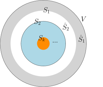
Figure 2: Contraction based decomposition for a submodular function $f$. Shown is the Venn-diagram of $S_{1},...,S_{k}$ and $\hat{S}_{1},...,\hat{S}_{k}$

See Figure 2 throughout this proof. Note that $\hat{S}_{1},...,\hat{S}_{k}$ are associated with densities

$$\frac{|V|-|S_{1}|}{f(V)-f(S_{1})}<\frac{|S_{1}|-|S_{2}|}{f(S_{1})-f(S_{2})}<...<\frac{|S_{k-1}|-|S_{k}|}{f(S_{k-1})-f(S_{k})}$$

Similarly, $T_{1},...,T_{k^{\prime}}$ are associated with densities

$$\frac{f(V)-f(V\setminus T_{1})}{|T_{1}|}>\frac{f(V\setminus T_{1})-f(V\setminus T_{1}\setminus T_{2})}{|T_{2}|}>...>\frac{f(T_{k^{\prime}})-f(\phi)}{|T_{k^{\prime}}|}$$

We prove the claim by induction. Suppose $T_{1},...,T_{i-1}$ is the same as $\hat{S}_{1},...,\hat{S}_{i-1}$ with the trivial base case.

First note that $T_{i}\subseteq S_{i-1}$ since $T_{1}\cup...\cup T_{i-1}=(V\setminus S_{1})\cup(S_{1}\setminus S_{2})\cup...(S_{i-2}\setminus S_{i-1})=V\setminus S_{i-1}$ and the disjointedness of $\{T_{j}\}$. Now observe that by the optimality of $S_{i}$ that

$$\frac{|S_{i-1}|-|S_{i}|}{f(S_{i-1})-f(S_{i})}\leq\frac{|S_{i-1}|-|S_{i-1}\setminus T_{i}|}{f(S_{i-1})-f(S_{i-1}\setminus T_{i})}=\frac{|T_{i}|}{f(S_{i-1})-f(S_{i-1}\setminus T_{i})}=\frac{|T_{i}|}{f(V\setminus\bigcup_{j<i}T_{j})-f(V\setminus\bigcup_{j\leq i}T_{j})}$$

Conversely, by the optimality of $T_{i}$

$$\frac{f(V\setminus\bigcup_{j<i}T_{j})-f(V\setminus\bigcup_{j\leq i}T_{j})}{|T_{i}|}\geq\frac{f(V\setminus\bigcup_{j<i}T_{j})-f(V\setminus\bigcup_{j<i}T_{j}\setminus(S_{i-1}\setminus S_{i}))}{|S_{i-1}\setminus S_{i}|}=\frac{f(S_{i-1})-f(S_{i})}{|S_{i-1}|-|S_{i}|}$$

Hence $\lambda_{i}=\hat{\lambda}_{i}$. This also forces $S_{i}=S_{i-1}\setminus T_{i}$ or $T_{i}=S_{i-1}\setminus S_{i}=\hat{S}_{i}$.

7.6 Proof of Lemma 4.2

Proof 7.6.

Consider the optimal orientation of the edges $d^{\ast}_{w}$. How does reversing one edge (from $(u,v)$ to $(v,u)$) affect the cost of minimization oracle? The out degree of $u$ decreases by $1$ and the out degree of $v$ increases by $1$, and so the objective function increases by $w_{v}-w_{u}$.

Suppose Weighted-Greedy++ peels the vertices $u_{1},...,u_{n}$ in this order. We proceed by induction. Consider all the “wrongly” oriented edges $W(u_{1})=\{(u_{1},u_{i}):i>1,w(u_{1})>w(u_{i})\}$. These edges increase the objective function from the optimal solution value by $\sum_{v\in W(u)}(w(u_{1})-w(v))$. But recall that Weighted-Greedy++ chooses $u_{1}$ because $w(u_{1})+deg_{G^{\prime}}(u_{1})\leq w(v)+deg_{G^{\prime}}(v)$ for all $v\in W(u)$. Which means that

$$w(u_{1})-w(v)\leq\deg_{G^{\prime}}(v)-deg_{G^{\prime}}(u_{1})\leq deg_{G}(v)$$

Proceeding by induction on $u_{2},...,u_{n}$, the “wrongly” oriented edges contribute a total of at most $\sum_{u}deg_{G}(u)^{2}$ additive error with respect to the correct orientation $d^{\ast}_{w}$ since each vertex $v$ contributes at most $deg_{G}(v)$ from all its neighbors.

7.7 Proof of Lemma 4.3

Proof 7.7.

Figure 3: Proof idea of Lemma Lemma 4.3

Suppose Weighted-SuperGreedy++ peels $V$ in the order $s_{i_{1}},...,s_{i_{n}}$, and Edmonds’ algorithm peels them in the order $s_{1},...,s_{n}$ with $w_{1}\leq...\leq w_{n}$. Let $A_{j}=\{s_{i_{j+1}},...,s_{i_{n}}\}$. Let $j$ be the index of the first disagreement where $s_{j}\neq s_{i_{j}}$. Weighted-SuperGreedy++ chooses $s_{i_{j}}$ over $s_{i_{k}}$ ($k\geq j$) because

$$w(s_{i_{j}})+f(s_{i_{j}}|A_{j}-s_{i_{j}})\leq w(s_{i_{k}})+f(s_{i_{k}}|A_{j}-s_{i_{k}})$$

Which implies by supermodularity

$$w(s_{i_{j}})-w(s_{i_{k}})\leq f(s_{i_{k}}\leavevmode\nobreak\ |\leavevmode\nobreak\ V-s_{i_{k}})$$ (6)

Suppose $s_{i_{k}}=s_{j}$, then we will move $s_{i_{j}},s_{i_{j+1}},...,s_{i_{k-1}}$ to go after $s_{i_{k}}=s_{j}$ in the Weighted-SuperGreedy++ order. (see Figure 3). Swapping consecutive elements $s_{i_{a}},s_{i_{a+1}}$ in the Weighted-SuperGreedy++ order changes the inner product cost by

$$w(s_{i_{a+1}})f(s_{i_{a+1}}|A_{a}+s_{i_{a}}-s_{i_{a+1}})+w(s_{i_{a}})f(s_{i_{a}}|A_{a+1})-w(s_{i_{a}})f(s_{i_{a}}|A_{a})-w(s_{i_{a+1}})f(s_{i_{a+1}}|A_{a+1})$$

$$=w(s_{i_{a}})(f(s_{i_{a}}|A_{a+1})-f(s_{i_{a}}|A_{a}))-w(s_{i_{a+1}})(f(s_{i_{a+1}}|A_{a+1})-f(s_{i_{a+1}}|A_{a}+s_{i_{a}}-s_{i_{a+1}}))$$ (7)

But

$$f(s_{i_{a}}|A_{a+1})-f(s_{i_{a}}|A_{a})=f(A_{a+1}+s_{i_{a}})-f(A_{a+1})-f(A_{a}+s_{i_{a}})+f(A_{a})$$

And

$$f(s_{i_{a+1}}|A_{a+1})-f(s_{i_{a+1}}|A_{a}+s_{i_{a}}-s_{i_{a+1}})=f(A_{a+1}+s_{i_{a+1}})-f(A_{a+1})-f(A_{a}+s_{i_{a}})+f(A_{a}+s_{i_{a}}-s_{i_{a+1}})$$

$$=f(A_{a})-f(A_{a+1})-f(A_{a}+s_{i_{a}})+f(A_{a+1}+s_{i_{a}})$$

And hence both coefficients of $w(s_{i_{a}}),w({s_{i_{a+1}}})$ in 7 are equal. Hence by (6)

$$(\ref{difference})=(w_{i_{a}}-w_{i_{a+1}})(f(s_{i_{a+1}}|A_{a+1})-f(s_{i_{a+1}}|A_{a+1}+s_{i_{a}}))\geq-f(s_{i_{a+1}}|V-s_{i_{a+1}})^{2}$$

Hence, moving all of $s_{i_{j}},...,s_{i_{k-1}}$ to $s_{i_{k}}=s_{j}$ decreases the cost by at most $\leq(k-j)f(s_{i_{k}}|V)^{2}\leq nf(s_{i_{k}}|V-s_{i_{k}})^{2}$. Summing over all reorderings of the vertices, we see that Edmonds’ ordering inner product is at most $n\sum_{u\in V}f(u|V-u)^{2}$ away from the Weighted-SuperGreedy++ order inner product. For the function $f(S)=|E(S)|$, the bound from Lemma 4.2 is better than the bound of Lemma Lemma 4.3 by a factor of $n$. We leave improving the bound for future work.

7.8 Proof of Lemma 5.1

Proof 7.8.

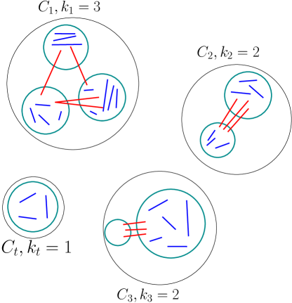
Figure 4: Blue edges are $S_{i}$. Red edges are $\hat{S}_{i}$. Red and blue edges together are $S_{i-1}$. The red edges in component $C_{q}$ are $E_{q}$. Cyan circles inside $C_{q}$ are components inside $C_{q}$ after $\hat{S}_{i}$ is deleted.

In the $i$-th iteration, observe that $\hat{S}_{i}=S_{i-1}\setminus S_{i}$ is just the edges crossing the partition $P(S_{i})$ in the graph $G^{\prime}=G(V,S_{i-1})$ remaining from iteration $i-1$. Also, $\frac{f(S_{i-1})-f(S_{i})}{|S_{i-1}|-|S_{i}|}=\frac{\kappa(S_{i})-\kappa(S_{i-1})}{E(P(S_{i}))}$. We show that this is the correct value consistent with Thorup’s ideal relative weights that the edges in $\hat{S_{i}}$ should be set to.

We proceed inductively on the $i$-th iteration.

Throughout the proof see Figure 4. Fix $G^{\prime}=G(V,S_{i-1})$. Let the connected components of $G^{\prime}$ be $C_{1},...,C_{t}$ with component $C_{q}$ having $k_{q}$ connected components after deleting $\hat{S}_{i}=S_{i-1}\setminus S_{i}$ and contributing edges $E_{q}$ to the cross edges in $\hat{S}_{i}$. Let $k=\sum_{i}k_{i}$.

If for some component $C_{q}$, we have $\frac{E_{q}}{k_{q}-1}<\frac{|S_{i-1}|-|S_{i}|}{k-1}$, then for $S_{i}^{\prime}=S_{i-1}\setminus E_{q}$, we have

$$\frac{|S_{i-1}|-|S_{i}^{\prime}|}{\kappa(S_{i-1}-\kappa(S_{i}^{\prime}))}=\frac{|E_{q}|}{k_{q}-1}<\frac{|S_{i-1}|-|S_{i}|}{k-1}$$

A contradiction to the optimality of $S_{i}$.

Hence, for all components $C_{q}$ with $k_{q}>1$, $\frac{E_{q}}{k_{q}-1}\geq\frac{|S_{i-1}|-|S_{i}|}{k-1}$. But then for $S_{i}^{\prime}=S_{i}\cup E_{q}$, we have

$$\frac{|S_{i-1}|-|S_{i}^{\prime}|}{\kappa(S_{i}^{\prime})-\kappa(S_{i-1})}=\frac{|S_{i-1}|-|S_{i}|-|E_{q}|}{\kappa(S_{i})-\kappa(S_{i-1})-k_{q}+1}\leq\frac{|S_{i-1}|-|S_{i}|}{\kappa(S_{i})-\kappa(S_{i-1})}$$

By optimality of $S_{i}$, equality must hold.

Hence it must be that if $k_{q}>1$ then $(k_{1}-1)/|E_{q}|=(k-1)/|\hat{S}_{i}|$. So the algorithm sets the correct densities for the edges in $\hat{S_{i}}$ according to Thorup’s algorithm.

References

- [1] Digvijay Boob, Yu Gao, Richard Peng, Saurabh Sawlani, Charalampos Tsourakakis, Di Wang, and Junxing Wang. Flowless: Extracting Densest Subgraphs Without Flow Computations, page 573–583. Association for Computing Machinery, New York, NY, USA, 2020.
- [2] Chandra Chekuri, Kent Quanrud, and Manuel R. Torres. Densest subgraph: Supermodularity, iterative peeling, and flow. In Proceedings of the 2022 Annual ACM-SIAM Symposium on Discrete Algorithms (SODA), pages 1531–1555, 2022.
- [3] Satoru Fujishige. Lexicographically optimal base of a polymatroid with respect to a weight vector. Mathematics of Operations Research, 5(2):186–196, 1980.
- [4] Marguerite Frank and Philip Wolfe. An algorithm for quadratic programming. Naval Research Logistics Quarterly, 3(1-2):95–110, 1956.
- [5] Martin Jaggi. Revisiting Frank-Wolfe: Projection-free sparse convex optimization. In Sanjoy Dasgupta and David McAllester, editors, Proceedings of the 30th International Conference on Machine Learning, number 1 in Proceedings of Machine Learning Research, pages 427–435, Atlanta, Georgia, USA, 17–19 Jun 2013. PMLR.
- [6] Elfarouk Harb, Chandra Chekuri, and Kent Quanrud. Faster and scalable algorithms for densest subgraph and decomposition.
- [7] Mikkel Thorup. Fully-dynamic min-cut. Combinatorica, 27(1):91–127, 2007. Preliminary version in Proc. of ACM STOC 2001.
- [8] Mikkel Thorup. Minimum k-way cuts via deterministic greedy tree packing. In Proceedings of the fortieth annual ACM symposium on Theory of computing, pages 159–166, 2008.
- [9] A. V. Goldberg. Finding a maximum density subgraph. Technical Report UCB/CSD-84-171, EECS Department, University of California, Berkeley, 1984.
- [10] Jean-Claude Picard and Maurice Queyranne. A network flow solution to some nonlinear 0-1 programming problems, with applications to graph theory. Networks, 12(2):141–159, 1982.
- [11] Alexander Schrijver et al. Combinatorial optimization: polyhedra and efficiency, volume 24. Springer, 2003.
- [12] Satoru Fujishige. Submodular functions and optimization. Elsevier, 2005.
- [13] Chenhao Ma, Yixiang Fang, Reynold Cheng, Laks V.S. Lakshmanan, Wenjie Zhang, and Xuemin Lin. Efficient algorithms for densest subgraph discovery on large directed graphs. In Proceedings of the 2020 ACM SIGMOD International Conference on Management of Data, SIGMOD ’20, page 1051–1066, New York, NY, USA, 2020. Association for Computing Machinery.
- [14] Maximilien Danisch, T.-H. Hubert Chan, and Mauro Sozio. Large scale density-friendly graph decomposition via convex programming. In Proceedings of the 26th International Conference on World Wide Web, WWW ’17, page 233–242, Republic and Canton of Geneva, CHE, 2017. International World Wide Web Conferences Steering Committee.
- [15] Charalampos Tsourakakis. The k-clique densest subgraph problem. In Proceedings of the 24th International Conference on World Wide Web, WWW ’15, page 1122–1132, Republic and Canton of Geneva, CHE, 2015. International World Wide Web Conferences Steering Committee.
- [16] Bintao Sun, Maximilien Danisch, T-H. Hubert Chan, and Mauro Sozio. Kclist++: A simple algorithm for finding k-clique densest subgraphs in large graphs. Proc. VLDB Endow., 13(10):1628–1640, jun 2020.
- [17] Reid Andersen and Kumar Chellapilla. Finding dense subgraphs with size bounds. In Konstantin Avrachenkov, Debora Donato, and Nelly Litvak, editors, Algorithms and Models for the Web-Graph, pages 25–37, Berlin, Heidelberg, 2009. Springer Berlin Heidelberg.
- [18] Charalampos Tsourakakis, Francesco Bonchi, Aristides Gionis, Francesco Gullo, and Maria Tsiarli. Denser than the densest subgraph: Extracting optimal quasi-cliques with quality guarantees. In Proceedings of the 19th ACM SIGKDD International Conference on Knowledge Discovery and Data Mining, KDD ’13, page 104–112, New York, NY, USA, 2013. Association for Computing Machinery.
- [19] Alessandro Epasto, Silvio Lattanzi, and Mauro Sozio. Efficient densest subgraph computation in evolving graphs. In Proceedings of the 24th International Conference on World Wide Web, WWW ’15, page 300–310, Republic and Canton of Geneva, CHE, 2015. International World Wide Web Conferences Steering Committee.
- [20] Andrew McGregor, David Tench, Sofya Vorotnikova, and Hoa T. Vu. Densest subgraph in dynamic graph streams. In Giuseppe F. Italiano, Giovanni Pighizzini, and Donald T. Sannella, editors, Mathematical Foundations of Computer Science 2015, pages 472–482, Berlin, Heidelberg, 2015. Springer Berlin Heidelberg.
- [21] Polina Rozenshtein, Nikolaj Tatti, and Aristides Gionis. Discovering dynamic communities in interaction networks. In Toon Calders, Floriana Esposito, Eyke Hüllermeier, and Rosa Meo, editors, Machine Learning and Knowledge Discovery in Databases, pages 678–693, Berlin, Heidelberg, 2014. Springer Berlin Heidelberg.
- [22] Oana Denisa Balalau, Francesco Bonchi, T-H. Hubert Chan, Francesco Gullo, and Mauro Sozio. Finding subgraphs with maximum total density and limited overlap. In Proceedings of the Eighth ACM International Conference on Web Search and Data Mining, WSDM ’15, page 379–388, New York, NY, USA, 2015. Association for Computing Machinery.
- [23] Yuko Kuroki, Atsushi Miyauchi, Junya Honda, and Masashi Sugiyama. Online dense subgraph discovery via blurred-graph feedback. In ICML, 2020.
- [24] Albert Angel, Nikos Sarkas, Nick Koudas, and Divesh Srivastava. Dense subgraph maintenance under streaming edge weight updates for real-time story identification. Proc. VLDB Endow., 5(6):574–585, feb 2012.
- [25] Kijung Shin, Tina Eliassi-Rad, and Christos Faloutsos. Corescope: Graph mining using k-core analysis — patterns, anomalies and algorithms. In 2016 IEEE 16th International Conference on Data Mining (ICDM), pages 469–478, 2016.
- [26] Xiangfeng Li, Shenghua Liu, Zifeng Li, Xiaotian Han, Chuan Shi, Bryan Hooi, He Huang, and Xueqi Cheng. Flowscope: Spotting money laundering based on graphs. In AAAI, 2020.
- [27] Tommaso Lanciano, Atsushi Miyauchi, Adriano Fazzone, and Francesco Bonchi. A survey on the densest subgraph problem and its variants, 2023.
- [28] Saurabh Sawlani and Junxing Wang. Near-optimal fully dynamic densest subgraph. In Konstantin Makarychev, Yury Makarychev, Madhur Tulsiani, Gautam Kamath, and Julia Chuzhoy, editors, Proccedings of the 52nd Annual ACM SIGACT Symposium on Theory of Computing, STOC 2020, Chicago, IL, USA, June 22-26, 2020, pages 181–193. ACM, 2020.
- [29] Aleksander B. G. Christiansen, Jacob Holm, Ivor van der Hoog, Eva Rotenberg, and Chris Schwiegelshohn. Adaptive out-orientations with applications, 2023.
- [30] Li Chen, Rasmus Kyng, Yang P. Liu, Richard Peng, Maximilian Probst Gutenberg, and Sushant Sachdeva. Maximum flow and minimum-cost flow in almost-linear time, 2022.
- [31] Moses Charikar. Greedy approximation algorithms for finding dense components in a graph. In Klaus Jansen and Samir Khuller, editors, Approximation Algorithms for Combinatorial Optimization, pages 84–95, Berlin, Heidelberg, 2000. Springer Berlin Heidelberg.
- [32] Fragkiskos D Malliaros, Christos Giatsidis, Apostolos N Papadopoulos, and Michalis Vazirgiannis. The core decomposition of networks: Theory, algorithms and applications. The VLDB Journal, 29(1):61–92, 2020.
- [33] Yuichi Asahiro, Kazuo Iwama, Hisao Tamaki, and Takeshi Tokuyama. Greedily finding a dense subgraph. Journal of Algorithms, 34(2):203–221, 2000.
- [34] Bahman Bahmani, Ashish Goel, and Kamesh Munagala. Efficient primal-dual graph algorithms for mapreduce. In International Workshop on Algorithms and Models for the Web-Graph, pages 59–78. Springer, 2014.
- [35] Digvijay Boob, Saurabh Sawlani, and Di Wang. Faster width-dependent algorithm for mixed packing and covering lps. Advances in Neural Information Processing Systems 32 (NIPS 2019), 2019.
- [36] H Narayanan. The principal lattice of partitions of a submodular function. Linear Algebra and its Applications, 144:179–216, 1991.
- [37] Hariharan Narayanan. Submodular functions and electrical networks, volume 54. Elsevier, 1997.
- [38] Satoru Fujishige. Theory of principal partitions revisited. Research Trends in Combinatorial Optimization: Bonn 2008, pages 127–162, 2009.
- [39] Nikolaj Tatti and Aristides Gionis. Density-friendly graph decomposition. In Proceedings of the 24th International Conference on World Wide Web, pages 1089–1099, 2015.
- [40] Nikolaj Tatti. Density-friendly graph decomposition. ACM Transactions on Knowledge Discovery from Data (TKDD), 13(5):1–29, 2019.
- [41] David R Karger. Minimum cuts in near-linear time. Journal of the ACM (JACM), 47(1):46–76, 2000.
- [42] Takuro Fukunaga. Computing minimum multiway cuts in hypergraphs from hypertree packings. In IPCO, pages 15–28. Springer, 2010.
- [43] Chandra Chekuri, Kent Quanrud, and Chao Xu. Lp relaxation and tree packing for minimum k-cut. SIAM Journal on Discrete Mathematics, 34(2):1334–1353, 2020.
- [44] Daniel Lokshtanov, Saket Saurabh, and Vaishali Surianarayanan. A parameterized approximation scheme for min k-cut. SIAM Journal on Computing, (0):FOCS20–205, 2022.
- [45] Jason Li. Faster minimum k-cut of a simple graph. In 2019 IEEE 60th Annual Symposium on Foundations of Computer Science (FOCS), pages 1056–1077. IEEE, 2019.
- [46] Anupam Gupta, David G Harris, Euiwoong Lee, and Jason Li. Optimal bounds for the k-cut problem. ACM Journal of the ACM (JACM), 69(1):1–18, 2021.
- [47] Jack Edmonds. Submodular functions, matroids, and certain polyhedra. In R. Guy, H. Hanani, N. Sauer, and J. Schönheim, editors, Combinatorial Structures and Their Applications (Proceedings Calgary International Conference on Combinatorial Structures and Their Applications, Calgary, Alberta, 1969; R. Guy, H. Hanani, N. Sauer, J. Schönheim, eds.), New York, 1970. Gordon and Breach.
- [48] Serge A. Plotkin, David B. Shmoys, and Éva Tardos. Fast approximation algorithms for fractional packing and covering problems. Mathematics of Operations Research, 20(2):257–301, 1995.
- [49] N. Young. Randomized rounding without solving the linear program. In ACM-SIAM Symposium on Discrete Algorithms, 1995.
- [50] Sanjeev Arora, Elad Hazan, and Satyen Kale. The multiplicative weights update method: a meta-algorithm and applications. Theory of computing, 8(1):121–164, 2012.