Exciton Diffusion in a Quantum Dot Ensemble

Abstract

We theoretically investigate the Förster transfer of an exciton in an ensemble of self-assembled quantum dots randomly distributed on a circular mesa. We use the stochastic simulation method to solve the equation of motion for the density matrix with a given decay rate. We express the diffusion in terms of the mean square displacement from the initially excited quantum dot. The mean square displacement follows three time stages: ballistic, normal diffusion, and saturation. In addition, the exciton exhibits power-law localization. Using an approximate analytical approach, we provide the formulas that follow the results of numerical studies.

I Introduction

Förster resonance energy transfer (FRET) appears widely in the quantum world, both in biological and technical structures. The former include light harvesting systems that employ cascade-like transport to move solar energy from pigment molecules to the reaction centers of photosynthesis [1, 2]. The latter are dominated by exciton diffusion in different types of quantum dots (QDs), e.g., QD solids [3], nanocrystals [4, 5], self-assembled QDs [6, 7, 8], and silicon QDs [9]. In particular, in Ref. [6] excitation transport has been observed in self-assembled QD ensembles with varying planar density. In that work, transport even beyond the excitation region was confirmed by the observed spatial width of photoluminescence (PL) that exceeded the excitation laser spot. Furthermore, an enhanced effect was observed in the case of diluted samples, eliminating the hypothetical possibility of carrier tunneling (Dexter transfer).

Energy transport in a QD ensemble involves the diffusion of an exciton, i.e. an electron-hole pair initially formed (e.g. optically) in individual QDs. The resonant energy transfer mechanism proposed by Förster [10, 11, 12] offers an explanation of transport in such systems. The excited donor-QD transfers its excitation to the remaining acceptor-QDs coupled via dipole interactions. Assuredly, the transport mechanism (Förster vs. Dexter) can be experimentally determined by analyzing the optical spectra in coherent two-dimensional spectroscopy [13].

The exact formula for Forster’s couplings in a planar set of dipole emitters (e.g. self-assembled QDs) is known. It was derived by transforming the minimal coupling Hamiltonian in a dipole approximation using the Power-Zienau-Wooley (PZW) transformation [14, 15, 16]. The resulting dipole-dipole power-law coupling has the form of a sum of three long-range terms decreasing with the distance, each multiplied by an oscillating factor [12, 17, 7, 8].

Self assembled QDs are not perfectly homogeneous (due to randomness of the growth process). Therefore, QDs differ in the fundalmental transition energy of forming an electron-hole pair. Such an energy dispersion makes the set of QDs a disordered system similar to that described by the Anderson tight-binding model [18, 19] with long-range hopping integral. Although most of the research on Anderson’s localization in disordered systems focused on nearest-neighbor-coupled models, Anderson’s original work dealt with long-range couplings, decreasing with some power of the intersite distance, $V(r)\propto r^{-\mu}$.

In this paper, we theoretically investigate the diffusion of a single exciton in a planar QD ensemble restricted to a circular mesa. Exciton diffusion is a manifestation of FRET that stems from long-range dipole-dipole couplings. The fundamental transition energy disorder has a negative impact on the range and speed of diffusion. A general framework for describing (quasi)particle diffusion in such systems was proposed in Ref. [20], where we investigated the diffusion of a single excitation on a regular one- or two-dimensional lattice with strong on-site disorder and inter-site coupling that decreases inversely proportionally with distance $V(r)\propto r^{-1}$. Here, we extend the considerations to a realistic system: a planar ensemble of randomly placed self-assembled quantum dots with fundamental transition energy disorder, coupled by the long-range oscillating Förster couplings. We also assume a finite exciton life-time and compare it to the idealized non-dissipative case. In order to simulate the dissipation process, we employ the numerical method of stochastic simulations, also known as the quantum jump method [21, 22].

The diffusion of an exciton is characterized by the mean-square displacement of the exciton as a function of time. We show that this quantity evolves in three steps: first ballistic motion, then standard diffusion, and finally saturation (cf. Ref. [20]). Similarly, the growth of the exciton density at a given QD follows three steps: quadratic in time, followed by linear in time ending in saturation. At the same time, the dependence of exciton density on the distance reveals power-law localization of the exciton in the system. We explain the three-step diffusion and power-law localization using a model in which the disorder expressed by the standard deviation of the transition energies is much greater than the coupling strength between sites [18, 20, 23]. In such a model system only first-order (direct) jumps from the excited site even to the remote ones are relevant. This regime is opposite to the nearest-neighbor coupled systems. By neglecting all the couplings except for those involving the initially occupied QD we are able to propose an approximate analytical solution to the exciton dynamics which, at least qualitatively, reproduces the simulation results. This allows us to gain a deeper understanding of the transport mechanism.

The organization of this paper is as follows. Sec. II contains a detailed description of the investigated system, the model that describes it, and the quantum jump method used for numerical simulations of the system dynamics. In Sec. III, we present the exciton dynamics obtained from the numerical evaluation of the introduced model. In Sec. IV, we propose an approximate analytical solution that reproduces the exciton dynamics. Finally, in Sec. V we conclude and discuss the results.

II System, Model and Simulation Method

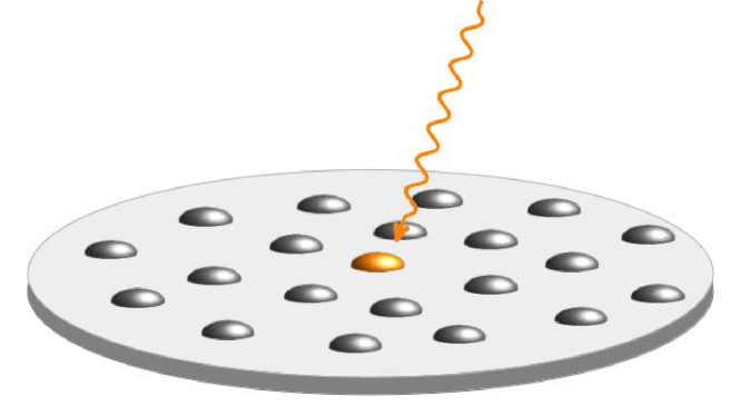
Figure 1: Schematic representation of the investigated system: planar ensemble of self-assembled QDs on circular mesa. The growth axis is perpendicular to the plane of the enseble. QD lying closest to the center is initially optically excited by circularly polarized light.

The system under study is a planar ensemble of self-assembled QDs randomly placed in the plane perpendicular to the growth axis (see Fig. 1) with constant surface density $\rho_{A}=10^{11}$ QDs$/$cm². In our model, QDs occupy a circular area of radius $R$. Due to the constant planar density, the number of QDs is adjusted to the linear size of the mesa and is approximately equal to $N=\rho_{A}\pi R^{2}$. That is, in the simulations, the number of QDs and the planar density $\rho_{A}$ are fixed, and the size of the mesa is adjusted. The average distance between the nearest sites is $r_{\mathrm{av}}\approx(\rho_{A})^{-1/2}\approx 32$ nm. However, the minimum distance between QDs is limited to $d_{\mathrm{min}}=10$ nm, which roughly corresponds to the minimum diameter of a single QD. The positions of the dots are denoted by $\bm{r}_{\alpha}$. The investigated system is not homogeneous. Quantum dots differ in their fundamental transition energy. We denote this energy by $E_{\alpha}=\overline{E}+\epsilon_{\alpha}$ for the $\alpha$-th QD, where $\overline{E}$ corresponds to its average, which is approximately $2.59$ eV using the value of the CdTe QD, and $\epsilon_{\alpha}$ is a small deviation from the average, modeled here by a symmetric normal distribution $\mathcal{N}(0,\sigma^{2})$ of the variation $\sigma^{2}$. The value of $\sigma$ is typically $\sim 50$ meV, however here we consider much more homogeneous systems. The highly uniform QDs fabricated by local droplet etching [24] evince a photoluminescence (PL) linewidth of less than 10 meV.

Although the size of a single QD is much smaller than the relevant radiation wavelength, the size of the ensemble can exceed it several times. Thus, the dipole approximation cannot be applied to the system as a whole. Instead, we employ the PZW transformation [14, 15, 16]. It converts the minimum-coupling Hamiltonian in the Coulomb gauge representing an ensemble of small physical systems into the Hamiltonian of quantum emitters treated as a point dipole each, coupled to the electric displacement field $\bm{\hat{D}}(\bm{r})$.

Then, the QD ensemble, together with the surroundings of the radiation and the interaction between them, is described by the Hamiltonian,

$$\hat{H}=\hat{H}_{\mathrm{at}}+\hat{H}_{\mathrm{rad}}+\hat{V}_{\textrm{at-rad}},$$ (1)

where

$$\hat{H}_{\mathrm{at}}=\sum_{\alpha}\epsilon_{\alpha}\hat{\sigma}^{\dagger}_{\alpha}\hat{\sigma}_{\alpha}$$ (2)

is the Hamiltonian of the dipole emitters (QDs) with $\hat{\sigma}_{\alpha}$ representing the transition operator that annihilates the excitation at the site $\alpha$. The second term corresponds to the photon bath,

$$\hat{H}_{\mathrm{rad}}=\sum_{\bm{k}\lambda}\hbar\omega_{k}\hat{b}^{\dagger}_{\bm{k}\lambda}\hat{b}_{\bm{k}\lambda},$$ (3)

where $\hat{b}_{\bm{k}\lambda}$ ($\hat{b}_{\bm{k}\lambda}^{\dagger}$) is the annihilation (creation) operator for photon of wave vector $\bm{k}$ and polarization $\lambda$, whereas $\omega_{k}$ is the corresponding photon frequency. The last term,

$$\hat{V}_{\textrm{at-rad}}=-\frac{1}{\varepsilon_{0}\varepsilon_{r}}\sum_{\alpha}\bm{\hat{d}}_{\alpha}\cdot\bm{\hat{D}}(\bm{r}_{\alpha}),$$ (4)

stems from the PZW transformation and corresponds to the coupling between the QDs and the electromagnetic field. Here, $\bm{\hat{d}}_{\alpha}=\bm{d}_{0}\hat{\sigma}_{\alpha}+\bm{d}^{*}_{0}\hat{\sigma}_{\alpha}^{\dagger}$ is the dipole moment operator for the emitter $\alpha$, while $\varepsilon_{0}$ and $\varepsilon_{r}$ are the electric permittivity of the vacuum and the material, respectively. Here, the dipole operator corresponds to creating a coherent superposition of bright excitons with total angular momentum $+1$ or $-1$ using circularly polarized light. In Appendix B, we have included some results from the enhanced model, in which we separately address both bright excitons together with the exciton fine structure splitting.

The displacement field is expressed by the photon operators as

$$\bm{\hat{D}}(\bm{r})=i~{}\sum_{\bm{k}\lambda}\sqrt{\dfrac{\hbar\varepsilon_{0}\varepsilon_{r}\omega_{k}}{2\mathcal{V}}}\hat{e}_{\bm{k}\lambda}\hat{b}_{\bm{k}\lambda}e^{i\bm{k}\cdot\bm{r}}+\mathrm{h.c.},$$ (5)

where the unit vector $\hat{e}_{\bm{k}\lambda}$ determines the polarization of light in the mode with wave vector $\bm{k}$ and polarization $\lambda$ and $\mathcal{V}$ is the normalization volume.

The equation of motion for the reduced density matrix $\rho$ can be derived following the steps of Ref. [12]. One first looks at the evolution of the quantum mechanical average of any operator $Q$ in the Heisenberg picture. Evolution is governed by a Hamiltonian, which includes both electronic and photonic degrees of freedom. The equation of motion of the atomic and photonic operators is found and the latter is then eliminated, leading to an integro-diffrential equation for the atomic operators which is reduced by using the Markov approximation. In the end, one neglects off-resonant terms and radiation-induced energy shifts and rewrites the equation in the Schrödinger picture obtaining the equation of motion (see also Refs. [8, 7]),

$$\frac{\differential}{\differential t}\hat{\rho}=-\dfrac{i}{\hbar}\left[\hat{H}_{0},\hat{\rho}\right]+\sum_{\alpha\beta}\Gamma_{\alpha\beta}\left(\hat{\sigma}_{\alpha}\hat{\rho}\hat{\sigma}_{\beta}^{\dagger}-\dfrac{1}{2}\left\{\hat{\sigma}^{\dagger}_{\beta}\hat{\sigma}_{\alpha},\hat{\rho}\right\}\right)$$ (6)

where

$$\hat{H}_{0}=\hat{H}_{\mathrm{at}}+\sum_{\alpha\beta}V_{\alpha\beta}^{(\mathrm{LR})}\hat{\sigma}^{\dagger}_{\alpha}\hat{\sigma}_{\beta}.$$ (7)

The first term on the right-hand side of Eq. (6) corresponds to the unitary dissipationless evolution of the system, whereas the second term is the Linblad part responsible for the dissipation process. The long-range coupling between the QDs is expressed by

$$V_{\alpha\beta}^{\mathrm{(LR)}}=-\hbar\Gamma_{0}G(k_{0}r_{\alpha\beta})$$ (8)

with $V_{\alpha\alpha}^{(\mathrm{LR})}=0$, where $\bm{r}_{\alpha\beta}=\bm{r}_{\alpha}-\bm{r}_{\beta}$, $\Gamma_{0}=|d_{0}|^{2}k_{0}^{3}/(3\pi\varepsilon_{0}\varepsilon_{r})$ is the spontaneous emission rate for a single dot and $k_{0}=2\pi n_{\mathrm{refr}}/\lambda_{0}=n_{\mathrm{refr}}\overline{E}/(\hbar c)$, where $n_{\mathrm{refr}}$ is the refractive index of the medium and $c$ denotes the speed of light. The values of these and other material parameters are gathered in Table 1. The coupling has a mixed power-law and oscillating character [12],

$$G(x)=-\dfrac{3}{8}\left(\dfrac{\cos x}{x}+\dfrac{\sin x}{x^{2}}+\dfrac{\cos x}{x^{3}}\right).$$ (9)

The short-range couplings provided by the overlap of the QDs wave functions and/or Coulomb correlations were neglected due to relatively large interdot distance (wave functions do not overlap). As was shown in Ref. [7] short-range interactions are responsible for collective emmision (superradiance) in the ensemble. They however cannot have significant impact on transport in a highly inhomogeneous ensemble.

The second term in Eq. (6) is responsible for the dissipation process. The dissipator coefficients are $\Gamma_{\alpha\alpha}=\Gamma_{0}$ and $\Gamma_{\alpha\beta}=\Gamma_{0}F(k_{0}r_{\alpha\beta})$, where

$$F(x)=\dfrac{3}{4}\left(\dfrac{\sin x}{x}-\dfrac{\cos x}{x^{2}}+\dfrac{\sin x}{x^{3}}\right),$$ (10)

cf. Refs. [7, 8].

Description	Symbol	Value	Unit
Spontaneous emission rate	$\Gamma_{0}$	1.0/0.39	ns-1
Resonance wave length (vacuum)	$\lambda_{0}$	479	nm
Refractive index	$n_{\mathrm{refr}}$	2.6	-
Surface density of QDs (2D)	$\rho_{A}$	$10^{11}$	cm-2
Minimal QD diameter	$d_{\mathrm{min}}$	10	nm

Table 1: Material parameters of the system.

To efficiently simulate systems of thousands of dots, we employ the quantum jump method [21, 22]. In this approach, we consider a state vector of $N$ elements instead of a density matrix of $N^{2}$ elements, which unburdens the computational load. The time-dependent state of the system $\ket{\Psi(t)}$ is expressed in the basis of the exciton located at a single dot $\{\ket{\alpha}\}_{\alpha=0}^{N-1}$,

$$\ket{\Psi(t)}=\sum_{\alpha}c_{\alpha}(t)\ket{\alpha},$$ (11)

where $c_{\alpha}(t)$ is the time-dependent probability amplitude for finding the exciton at the site $\alpha$. For dissipationless systems, one can reduce the equation of motion [Eq. (6)] to the first term, which yields a Schrödinger equation that can be solved by exact diagonalization of the Hamiltonian (7), see Ref. [20].

Stochastic simulation method

Now we briefly summarize the stochastic simulation method. A detailed description of this method can be found in Refs. [21, 22]. The method is based on the conversion of the master equation [Eq. (6)] into a piecewise continuous stochastic process. Let us start by transforming Eq. (6) into the equivalent form,

$$\frac{\differential}{\differential t}\hat{\rho}=-\frac{i}{\hbar}\left(\hat{H}_{\mathrm{eff}}\hat{\rho}-\hat{\rho}\hat{H}_{\mathrm{eff}}\right)+\sum_{i=1}^{N}\tilde{\Gamma}_{i}\tilde{\sigma}_{i}\hat{\rho}\tilde{\sigma}_{i}^{\dagger},$$ (12)

where

$$\hat{H}_{\mathrm{eff}}=\hat{H}_{0}+\frac{\hbar}{2i}\sum_{\alpha\beta}\Gamma_{\alpha\beta}\hat{\sigma}_{\alpha}^{\dagger}\hat{\sigma}_{\beta}$$ (13)

is the effective non-Hermitian Hamiltonian which governs the stochastic evolution between jumps and where $\tilde{\Gamma}_{i}$ are the eigenvalues of the dissipator $\Gamma_{\alpha\beta}$. The corresponding eigenvectors are denoted by $u_{i}=(u_{i,\alpha})_{\alpha=0}^{N-1}$ and

$$\tilde{\sigma}_{i}=\sum_{\alpha}u_{i,\alpha}^{*}\hat{\sigma}_{\alpha}.$$ (14)

The unnormalized state $\ket{\Psi(t)}$ [Eq. (11)] evolves according to the Schrödinger equation

$$i\hbar\frac{\differential}{\differential t}\ket{\Psi(t)}=H_{\mathrm{eff}}\ket{\Psi(t)}$$ (15)

until the jump occurs. The time interval between jumps is a random variable with a cumulative distribution function $\mathcal{F}(t)=1-\innerproduct{\Psi(t)}{\Psi(t)}$. While continuous evolution preserves the number of excitons, each jump corresponds to the emission of a single photon. In the case of multiple excitations present in the system, many jumps divided by continuous processes can occur. Here, we restrict ourselves only to the single exciton initial state, which prohibits further evolution after the first jump. The evolution of state $\ket{\Psi(t)}$ is calculated numerically according to Eq. (15). At each time step, one checks if the jump is to occur by comparing the current time with the jump time drawn from the distribution $\mathcal{F}(t)$. At a jump, the state ket is transformed according to

$$\ket{\Psi}\longrightarrow\frac{\sqrt{\tilde{\Gamma}_{i}}\tilde{\sigma}_{i}\ket{\Psi}}{\Bigl{|}\sqrt{\tilde{\Gamma}_{i}}\tilde{\sigma}_{i}\ket{\Psi}\Bigr{|}^{1/2}},$$ (16)

which in our case (single exciton) is just $\ket{\Psi}\rightarrow 0$. The simulation is performed multiple times for different disorder realizations of the energy and positions of QDs, as well as the random jump process. Then the desired quantity is averaged over the repetitions.

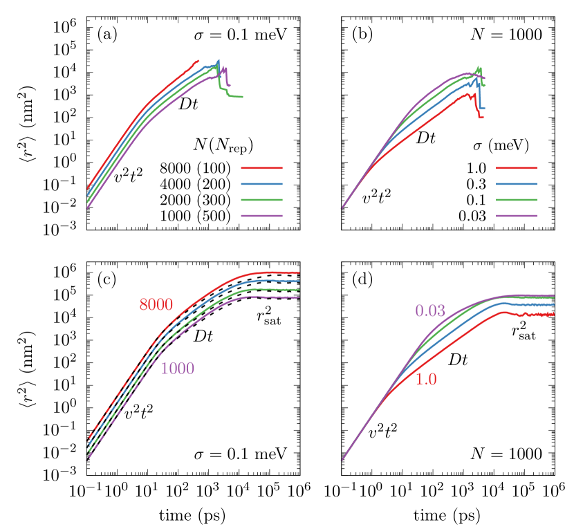
Figure 2: Mean square displacement of the exciton as a function of time for dissipative (a,b) and idealized nondissipative system (c,d) for different values of the system size and disorder strength. The number of realizations $N_{\mathrm{rep}}$ is given in the legend of panel (a) in paranthesis for each system size.

Quantities describing the dynamics

For a quantitative characterization of the diffusion, we are first interested in the spatial and temporal dependence of the occupation density, $\varrho_{\Delta r}(t,r)$, which is a normalized histogram of the occupation $\langle|c_{\alpha}(t)|^{2}\rangle_{r,\epsilon}$ where in each interval $\Delta r$ we count the occupations of QDs lying between $r$ and $r+\Delta r$, with $\Delta r=5$ nm. $\langle\dots\rangle_{r,\epsilon}$ corresponds to the average of $N_{\mathrm{rep}}$ realizations in which each time we set different random positions $\bm{r}_{\alpha}$ and random energies $\epsilon_{\alpha}$.

We also look for the mean square displacement (MSD) of the exciton from the center of the mesa structure, where it was initially created,

$$\bigl{\langle}r^{2}(t)\bigr{\rangle}_{r,\epsilon}=\biggl{\langle}\sum_{\alpha}r_{\alpha}^{2}\bigl{|}c_{\alpha}(t)\bigr{|}^{2}\biggr{\rangle}_{r,\epsilon},$$ (17)

where $r_{\alpha}\equiv|\bm{r}_{\alpha 0}|=|\bm{r}_{\alpha}-\bm{r}_{0}|$ is the distance from the QD initially occupied ($\alpha=0$).

In addition to that, we model the temporal dependence of the PL intensity. In each of the $N_{\mathrm{rep}}$ realizations, we record the timestamp of the emission jump, and on the basis of that, we form a histogram of a number of jumps in each time period $\Delta t$. The PL intensity is proportional to

$$I\propto\frac{\langle N_{\mathrm{ex}}\rangle_{r,\epsilon}}{N_{\mathrm{rep}}\Delta t}$$ (18)

where $\langle N_{\mathrm{ex}}\rangle_{r,\epsilon}$ is the number of light quanta emitted in the time $[t,t+\Delta t)$ averaged over the realizations. The time interval varies appropriately to achieve equal spacing on a logarithmic scale.

All the results obtained for the dissipative system employ the quantum jump method. On the contrary, for dissipationless systems, we use exact diagonalization to solve the unitary equation of motion given by the first term in right-hand side of Eq. (6).

III Results of the numerical simulations

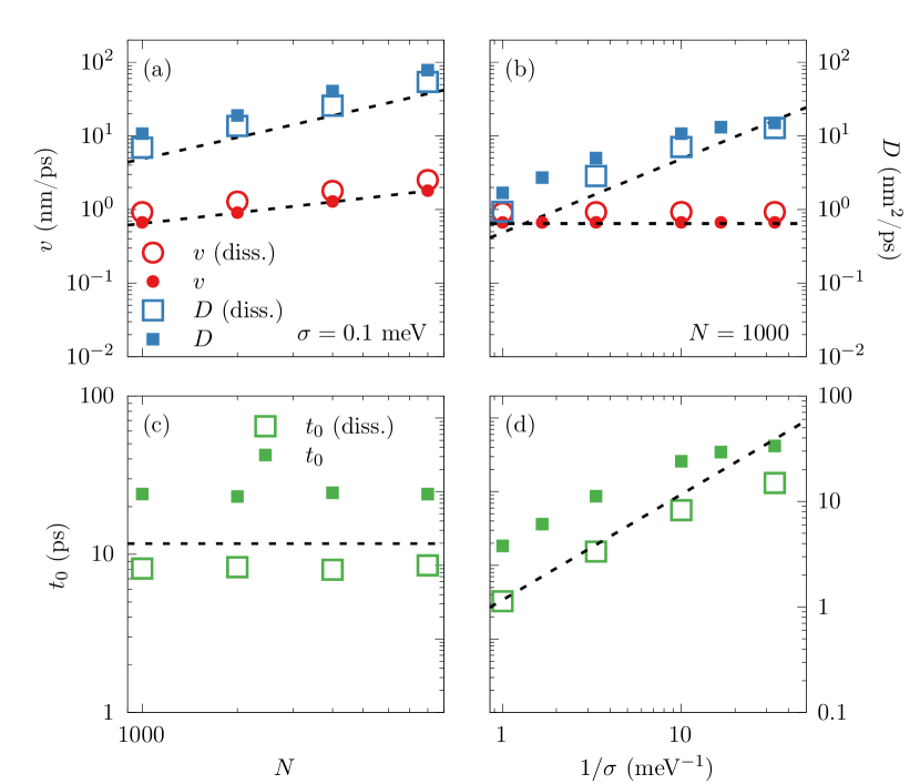
Figure 3: (a,b) Velocity of the ballistic motion (in red) and diffusion coefficient of normal diffusion (in blue) as a function of the system size and inverse disorder respectively; (c,d) crossover time between ballistic and diffusive stages (in green) as a function of the system size and inverse disorder strength, respectively. Open symbols correspond to the dissipative system whereas solid symbols to the idealized nondissipative system. Dashed lines respond for the approximate analytical results, see Sec. IV.

In this section, we present the results obtained by a numerical implementation of the model presented in Sec. II. Specifically, we present the temporal evolution of MSD [Eq. (17)] comparing the system of a realistic limited exciton lifetime with an idealistic non-dissipative system. We also present the spatial distribution of exciton occupations $\mathrm{X}_{\mathrm{num}}=\langle\absolutevalue{\innerproduct{\Psi}{\Psi}}^{2}\rangle_{r,\epsilon}$ in the ensemble and reveal the PL intensity.

Three-step dynamics

Fig. 2 shows MSD [Eq. (17)] as a function of time for dissipating systems [panels (a) and (b)] and dissipation-free systems [panels (c) and (d)] for several values of system size $N$ and standard deviation $\sigma$ of fundamental transition energy mismatch $\epsilon_{\alpha}$. Straight lines on a doubly logarithmic scale indicate the power-law dependencies of the MSD on time. MSD evolves in three subsequent steps. First, for very short times, we observe ballistic transport with constant velocity $v$,

$$\bigl{\langle}r^{2}(t)\bigr{\rangle}_{r,\epsilon}=v^{2}t^{2},\quad t<t_{0}.$$ (19)

Then, at a certain point in time $t_{0}$, standard diffusion with an appropriate diffusion constant $D$ starts,

$$\bigl{\langle}r^{2}(t)\bigr{\rangle}_{r,\epsilon}=Dt,\quad t_{0}<t<t_{1}.$$ (20)

Finally, at some time $t_{1}$, MSD saturates.

$$\bigl{\langle}r^{2}(t)\bigr{\rangle}_{r,\epsilon}=r_{\mathrm{sat}}^{2},\quad t_{1}<t,$$ (21)

which is only visible in an idealized system with an infinite exciton lifetime [Fig. 2(c,d)]. Otherwise, the exciton decays before saturation is reached. From the requirement for the MSD to be a continuous function, one gets the crossover time between the ballistic and diffusive phases,

$$t_{0}=D/v^{2},$$ (22)

as well as the crossover time between the standard diffusion and saturation stages,

$$t_{1}=r_{\mathrm{sat}}^{2}/D.$$ (23)

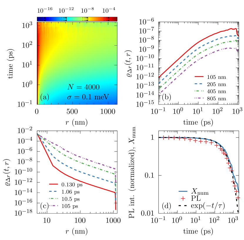
Figure 4: (a) Color-map of an occupation density $\varrho_{\Delta r}(t,r)$ as a function of time and distance from the central QD. For the sake of clarity, the data was truncated not to cover noise points after exciton recombination ($t\gtrsim 4\tau$); (b) Temporal evolution of $\varrho_{\Delta t}(t,r)$ for a few values of the distance from the center [the lines correspond to the vertical sections of the panel (a)]. (c) Distance dependence of $\varrho_{\Delta t}(t,r)$ for a few values of time [the lines correspond to the horizontal sections of the panel (a)]. (d) Photoluminescence intensity (see Eq. (18)) and exciton decay in time. The dashed line represents the ideal exponential decay with decay time $\tau=390$ ps as assumed in the simulations.

Dynamical parameters

We found the dynamical parameters of diffusion, that is, the ballistic velocity $v$ and the diffusion coefficient $D$ (for dissipative and idealized systems) together with the diffusion range $r_{\mathrm{sat}}^{2}$ (only for idealized systems), and crossing times $t_{0}$ and $t_{1}$ by fitting the appropriate power functions to the corresponding stages of motion [Eqs. (19)–(21)]. In addition, the saturation level can be found directly from the exact diagonalization of (7) which we explain in the Appendix A.

In Fig. 3 we present the dependence of the velocity and diffusion coefficient on the size of the system and the strength of the energy disorder. The dependencies seem to follow power laws with an integer or a simple rational exponent. The velocity grows as the square root of the size of the system [$v\propto N^{0.481\pm 0.011}$ from the fitting; see Fig. 3(a)] and is independent of the disorder [Fig. 3(b)]. The diffusion coefficient increases linearly with the size of the system [$D\propto N^{0.969\pm 0.037}$ from fitting, see Fig. 3(a)], but decreases with the disorder strength as $\propto 1/\sigma$ [$D\propto\sigma^{-0.955\pm 0.012}$ from fitting, Fig. 3(b)] at least for a strong disorder. As the disorder decreases, the diffusive stage becomes less and less visible. It is reflected in the dependence of diffusion coefficient $D$ in Fig. 3(b), which deviates from the trend $1/\sigma$ for decreasing disorder (right part of the panel).

Dissipation changes the values of the ballistic velocity and the diffusion coefficient. In Fig. 3(a) and Fig. 3(b) one notices that the ballistic velocity in the dissipative system is larger by a constant multiplicative factor compared to the velocity in the idealized system. It follows that dissipation leads to an acceleration of diffusion in its first stage. This means a faster emptying of the central QDs in favor of the other dots in the system. On the contrary, in the second phase of motion, the diffusion coefficient in the idealized system exceeds the diffusion coefficient in the dissipative system by a constant multiplicative factor [Fig. 3(a) and Fig. 3(b)]. This means that dissipation causes diffusion to slow down in the second phase of motion.

Exciton spacial distribution

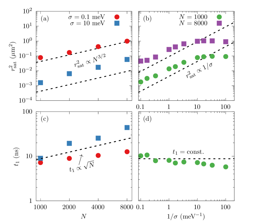
Figure 5: (a,b) The level of saturation of mean square displacement as a function of the size of the system (a) and inverse disorder strength (b), respectively. (c,d) Crossover time, at when the saturation stage begins, similarly as a function of the size of the system (c), and inverse disorder strength (d), respectively. The data was obtained mostly by numerical fit to MSD. Only the violet squares in panel (b) were obtained via exact diagonalization method explained in Appendix B

In Fig. 4(a), we see a color map of the temporal and spatial dependence of the occupation density $\mathcal{\varrho}_{\Delta r}(t,r)$. Separately, we illustrate how the occupation density at certain distances grows in time [Fig. 4(b)] and how occupations are distributed in space for several values of time [Fig. 4(c)]. The data are presented for a dissipative system. The occupation at each length follows three steps similar to MSD: first, quadratic in time, then linear in time, and finally saturates. The spatial decay of $\varrho_{\Delta r}(t,r)$ can be considered as a power law with different power exponents: higher for close QDs than for remote ones. In Table 2 we gather these exponents in the long-distance regime, corresponding to the subsequent curves in Fig. 4(c). The value of the exponent is close to $-2$, which is consistent with the analytical solution presented in Sec. IV.

time (ps)	exponent $\mu$
$0.13$	$-2.1147\pm 0.0098$
$1.06$	$-2.1213\pm 0.0097$
$10.54$	$-2.1715\pm 0.0089$
$104.82$	$-2.194\pm 0.022$

Table 2: The exponent of the power-law distribution of the exciton occupation density [see Fig. 4(c)] in the limit of long distance from the central QD, $\propto r^{\mu}$.

Diffusion range

It is clear from Fig. 2 that the exciton life is too short to reach saturation. Therefore, we determine the extent of diffusion for the idealized case of no dissipation. The saturation level shown in Fig. 5(a) increases with the number of dots in the system as $\propto N^{3/2}$, which implies an increase as $\propto R^{3}$. This trend cannot continue for large systems because the MSD increases faster than $\propto R^{2}$. This may mean that the exciton will reach the mesa border for some value of $N$ and the subsequent growth will continue with the trend $\propto R^{2}$. This change should be visible for homogeneous systems; however, even for $\sigma=0.1$ meV the trend is still $N^{3/2}$ [Fig. 5(a), see last paragraph of Section IV for a discussion].

The diffusion range of a single exciton is about $100$ nm [Fig. 2(a,b)], which corresponds to a time of several nanoseconds. Excitation spreads throughout the system, as shown in Fig. 4(a), the population of distant dots is small, less than $10^{-8}$. However, in the $100$ nm region around the excitation center a few nanoseconds after excitation, the occupancies remain at the level of $\sim 10^{-4}$. The photoluminescence intensity shown in Fig. 4(d) as a function of time is still not negligible for this time-space regime.

Photoluminescence & occupation decay

The time dependence of the PL intensity and the total exciton occupation are presented in Fig. 4(d). Both exhibit nearly exponential decay. The numerical fit of the function $\exp(t/\tau)$ in an interval $[0,2\tau]$ gives an exciton decay time of $\tau_{X}=(435.2\pm 2.5)$ ps and PL decay time $\tau_{\text{PL}}=(279\pm 12)$ ps. Therefore, from the beginning of evolution, while exciton decays slower, PL decays faster than the independent emitter ($\tau=390$ ps). However, at later times, the PL intensity slows down, even below the independent QD rate that is seen in Fig. 4(d) (red crosses on the right-hand side of the panel). In Ref. [7] Kozub et al. it was suggested that the enhanced emission is caused by short-range couplings due to tunneling and Coulomb correlations. The long-range couplings are too weak to impact emission in a strongly disordered ensemble. However, in the case of a homogeneous system ($0.1$ meV in Fig. 4) the Förster couplings start to play a role, which is visible in the change of the ensemble emission against the emission of the independent emitters.

The central atom model

At the end of this section, we would like to introduce the following observation (cf. Ref. [20, 23]). In Fig. 2(c) dashed lines indicate the results of numerical simulations made in the first-order approximation (which we refer to as the central atom model) in which only direct couplings from central QD are relevant, while the other are set to zero. The data follow the solution of the full model especially in the ballistic and diffusive stages of motion and deviate slightly in the saturation regime. This approximation is justified when the strength of the disorder is much greater than the Förster coupling between QDs and the size of the system is not too big. The central atom model allows one to analytically approximate the full model solution, which is the subject of the next section.

IV Approximate analytical approach

In this section, we present an approximate analytical solution to the model presented in Sec. II that qualitatively reproduces the results of numerical studies obtained in Sec. III. This analytical approach was previously introduced in two different ways in Refs. [20] and [23] for a general lattice model of $N$ sites with long-range power-law coupling, $V(r)\propto 1/r$ in Ref. [20] and, more generally, for $V(r)\propto 1/r^{\mu}$ in Ref. [23]. Here, we extend that analytic approach to ensembles with randomly placed QDs and the oscillating three-term dipole coupling of Eqs. (8) and (9).

Excitonic occupation

Due to the symmetry of the central atom model, all QDs distant by $r$ from the center should have on average the same occupation $\langle|c_{r}(t)|^{2}\rangle_{\epsilon}$. It can be found by solving analytically the Anderson locator expansion [18], which becomes possible in the central atom model, as was done in Ref. [20]. However, in Ref. [23] we showed that the solution is the same if we consider only two sites coupled via long-range coupling $V(r)$. During the derivations, we assumed that the eigenenergies $z_{\alpha}$ can be assigned to the given QD as long as they only slightly deviate from the value of the fundamental transition energy $\epsilon_{\alpha}$ in each dot (diagonal disorder energy). This means that the magnitude of separation of the eigenenergy $|\delta z_{\alpha}|=|z_{\alpha}-z_{0}|$ is much greater than the separation between the eigen- and the bare energy $|z_{\alpha}-\epsilon_{\alpha}|$. In that way we obtain the exciton occupation of a QD distant by $r$ from the initially excited dot (before the ensemble average is made),

$$\bigl{|}c_{r}(t)\bigr{|}^{2}=V^{2}(r)h\bigl{(}t;\delta z_{r}\bigr{)},$$ (24)

with

$$h(t;x)=\dfrac{\sin^{2}\bigl{[}xt/(2\hbar)\bigr{]}}{\bigl{(}x/2\bigr{)}^{2}},$$ (25)

where the index $r$ in $\delta z_{r}=z_{r}-z_{0}$ refers to the dots distant by $r$ from the center. Eq. (24) does not include the effect of dissipation. The random positions of QDs and transition energies are independent random variables; therefore, we can separately evaluate the corresponding averages $\langle\dots\rangle_{\epsilon}$ and $\langle\dots\rangle_{r}$. The average $\langle\dots\rangle_{\epsilon}$ of the realizations of the energy disorder can be evaluated as integral with the probability density function $f_{r}(x)$ of $\delta z_{r}$,

$$\bigl{\langle}|c_{r}(t)|^{2}\bigr{\rangle}_{r,\epsilon}=\bigl{\langle}V^{2}(r)\bigr{\rangle}_{r}\int\limits_{-\infty}^{\infty}dx\bigl{\langle}f_{r}(x)\bigr{\rangle}_{r}h(t;x)\differential x.$$ (26)

The probability density $f_{r}(x)$ is close to the density of diagonal energy separation $f_{\infty}(x)$, which is a normal distribution of zero mean and standard deviation $\sqrt{2}\sigma$, but includes a narrow gap around zero of width $4|V(r)|$ reflecting the levels repulsion (see Fig. 6) [20, 23]. The index “$\infty$” refers to the infinite distance between QDs that corresponds to the lack of coupling, which implies $\delta z=\delta\epsilon$. When coupling is present, two sites of bare energy separation $\delta\epsilon$ contribute to two eigenvalues of separation $\delta z=\sqrt{\delta\epsilon+4V^{2}(r)}$. Taking advantage of this, we find that

$$\begin{aligned} f_{r}(x)&=\frac{\differential}{\differential x}\int\limits_{-\infty}^{\sqrt{x^{2}-4V_{r}^{2}}}\differential\overline{x}f_{\infty}(\overline{x})\\ &=f_{\infty}\left(\sqrt{x-4V^{2}(r)}\right)\frac{\absolutevalue{x}}{\sqrt{x^{2}-4V^{2}(r)}}\end{aligned}$$ (27)

for $\absolutevalue{x}>2|V(r)|$ and zero otherwise. Since $\langle V(r)\rangle_{r}=0$ and $f_{r}(x)$ is a function of $V^{2}(r)$ we separated the averages over the coordinate disorder in Eq. (26). We should now consider the form of $\langle V^{2}(r)\rangle_{r}$. $V^{2}(r)$ is a sum of six terms with different power exponents of distance (from $2$ to $6$) each multiplied by an oscillating factor. When averaging, we replace the oscillating numerators by their average over one period $\delta r=2\pi/k_{0}=\lambda/n_{\mathrm{refr}}\approx 184$ nm. Then we are left only with three terms with even exponents, i.e.,

$$\bigl{\langle}V^{2}(r)\bigr{\rangle}_{r}=\left(\hbar\Gamma_{0}\right)^{2}\widetilde{G}^{2}(k_{0}r)$$ (28)

with

$$\widetilde{G}^{2}(x)=\frac{9}{64}\Biggl{[}\frac{1}{2}\frac{1}{x^{2}}+\frac{3}{2}\frac{1}{x^{4}}+\frac{1}{2}\frac{1}{x^{6}}\Biggr{]}.$$ (29)

This approximation is rather rough for small distances, since the average distance between QDs is $32$ nm $\ll\delta r$. However, as long as the system is large and transport is dominated by direct Förster jumps to remote dots, this approximation will lead to at least quantitatively correct analytical formulas.

Mean square displacement

For systems with spherical symmetry, MSD [Eq. (17)] can be expressed as

$$\bigl{\langle}r^{2}(t)\bigr{\rangle}_{r,\epsilon}=\biggl{\langle}\sum_{r}r^{2}\sum_{k=1}^{n_{r}}\bigl{|}c_{r}^{(k)}(t)\bigr{|}^{2}\biggr{\rangle}_{r,\epsilon},$$ (30)

where the first sum runs through distances from the center, and the second sum passes over the $n_{r}$ QDs lying on a thin ring of radius $r$ in the ensemble. In the continuous limit of spatial distribution QDs with constant surface density $\rho_{A}$, Eq. (30) takes the form of

$$\bigl{\langle}r^{2}(t)\bigr{\rangle}_{r,\epsilon}=2\pi\rho_{A}\int\limits_{0}^{R}r^{3}\bigl{\langle}|c_{r}(t)|^{2}\bigr{\rangle}_{r,\epsilon}\differential r,$$ (31)

where the integration covers the circular area of the mesa of radius $R$. The index $k$ can be omitted due to the symmetry of the central atom model, that is, all QDs distant from the center by $r$ should have (on average) the same occupation. Evaluation of (26) and then (31) relies on dividing the evolution into three time regimes: for very short times, for moderate times, and finally for long times.

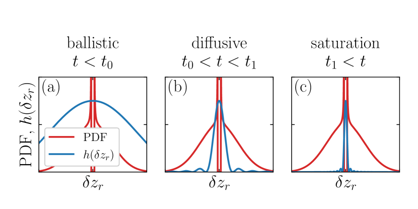
Figure 6: The probability density function (PDF) of eigenvale separation in the central atom model (the same red curve in each panel) versus the function $h(t,\delta z_{r})$ of Eq. (24) (blue curves). Panels correspods to ballistic (a), diffusive (b) and stauration (c) stages of evolution.

Ballistic motion

For very short times, $t<\hbar/\sigma$, $h(t;x)$ is broad and slowly varying [cf. Fig. 6(a)], hence it can be expanded into a Taylor series of first order around $t=0$, which yields $h(x)\approx t^{2}/\hbar^{2}$. In this case, the internal gap in the distribution does not have an important effect and can be neglected, thus $f_{r}(x)\approx f_{\infty}(x)=\exp[-x^{2}/(4\sigma^{2})]/\left(2\sqrt{\pi}\sigma\right)$ and the integration in (26) yields

$$\bigl{\langle}|c_{r}(t)|^{2}\bigr{\rangle}_{r,\epsilon}=\bigl{\langle}V^{2}(r)\bigr{\rangle}_{r}\frac{t^{2}}{\hbar^{2}}\quad\text{for}\quad t<t_{0}.$$ (32)

Furthermore, we evaluate (31), which takes the form

$$\bigl{\langle}r^{2}(t)\bigr{\rangle}=\left(\frac{2\pi\rho_{A}}{\hbar^{2}}\int r^{3}\langle V^{2}(r)\rangle_{r}\differential r\right)t^{2},$$ (33)

where the expression in parentheses is the squared ballistic velocity [Eq. (19)],

$$\begin{aligned} v^{2}=&\frac{9\Gamma_{0}^{2}}{128k_{0}^{2}}N+\frac{27\Gamma_{0}^{2}\pi\rho_{A}}{64k_{0}^{4}}\left[\ln(k_{0}R)-\ln(k_{0}r_{\mathrm{av}})\right]\\ &+\frac{9\Gamma_{0}^{2}\pi\rho_{A}}{128k_{0}^{4}}\left[\frac{1}{k_{0}^{2}r_{\mathrm{av}}^{2}}-\frac{1}{k_{0}^{2}R^{2}}\right].\end{aligned}$$ (34)

Standard diffusion

As time grows, $h(t;x)$ narrows. At moderate times, $\hbar/\sigma<t<\hbar/\sqrt{\langle V^{2}(R)\rangle_{r}}$, $h(x)$ becomes proportional to the unormalized Dirac delta of the area $2\pi t/\hbar$ but is still wide enough to be insensitive to the gap in $\langle f_{r}(x)\rangle_{r}$. Thus, we again approximate $\langle f_{r}(x)\rangle_{r}\approx f_{\infty}(x)$ and obtain the occupation,

$$\begin{aligned} \bigl{\langle}|c_{r}(t)|^{2}\bigr{\rangle}_{r,\epsilon}&=\bigl{\langle}V^{2}(r)\bigr{\rangle}_{r}\int\limits_{-\infty}^{\infty}\differential xf_{\infty}(x)2\pi\delta(x)/\hbar\\ &=\bigl{\langle}V^{2}(r)\bigr{\rangle}\frac{\sqrt{\pi}t}{\hbar\sigma}\quad\text{for}\quad t_{0}<t<t_{1}.\end{aligned}$$ (35)

Again we evaluate Eq. (31) and obtain MSD for the diffusive stage of motion [Eq. (20)], with the diffusion coefficient,

$$D=\frac{\sqrt{\pi}\hbar}{\sigma}v^{2}\propto\frac{N}{\sigma}.$$ (36)

The crossover time between the first and the second stage is

$$t_{0}=\frac{\sqrt{\pi}\hbar}{\sigma}.$$ (37)

The analytical formulas for $v$, $D$, and $t_{0}$ are represented by a dashed line in Fig. 3. They provide trends that are at least qualitatively aligned with the numerical data.

Saturation. The diffusion range

Finally, we find the diffusion range expressed by the saturation level of MSD. For distant times, $t>\hbar/\sqrt{\langle V^{2}(R)\rangle}$, the central peak of $h(x)$ falls into the gap inside $\langle f_{r}(x)\rangle_{r}$. The peak is canceled, and the remaining part of $h(x)$ can be approximated by $h(x)\approx 1/(2x^{2})$ where the oscillating nominator was averaged over its period. We evaluate (31) and obtain

$$\begin{split}\bigl{\langle}|&c_{r}(\infty)|^{2}\bigr{\rangle}_{r,\epsilon}=\\ &=\frac{\sqrt{\pi}}{2\sigma}\sqrt{\langle V^{2}(r)\rangle_{r}}\operatorname{erfc}\left(\frac{\sqrt{\langle V^{2}(r)\rangle_{r}}}{\sigma}\right)\exp\left(\frac{\langle V^{2}(r)\rangle_{r}}{\sigma^{2}}\right)\\ &\approx\frac{\sqrt{\pi}}{2\sigma}\sqrt{\langle V^{2}(r)\rangle_{r}}\quad\text{for}\quad t_{1}<t.\end{split}$$ (38)

Next, we calculate the diffusion range using Eq. (31) which takes the form

$$r^{2}_{\mathrm{sat}}=\frac{\pi^{3/2}\rho_{A}}{\sigma}\int r^{3}\sqrt{\langle V^{2}(r)\rangle}\differential r.$$ (39)

The integrand in (39) is a square root of a polynomial of $r$. In general, the integral can be expressed using elliptic functions of the first and second types. However, such a result is impractical and it is difficult to extract a trend in $R$ from it. For simplicity, let us approximate the integral in Eq. (39) by keeping only the largest term in the integrand, that is, proportional to $r^{2}$ (in the regime of large ensembles, $R\gg 1/k_{0}$). Then we obtain

$$\begin{aligned} r^{2}_{\mathrm{sat}}=&\frac{\sqrt{2}\pi^{3/2}\rho_{A}}{16}\frac{\hbar\Gamma_{0}}{\sigma k_{0}}R^{3}=\frac{\sqrt{2}}{16\sqrt{\rho_{A}}}\frac{\hbar\Gamma_{0}}{\sigma k_{0}}N^{3/2}\\ &\approx 0.138\frac{N^{3/2}}{\sigma[\text{meV}]}[\text{nm}].\end{aligned}$$ (40)

This result provides a growth of the diffusion range a $N^{3/2}$, which is consistent with the simulation results in Fig. 5(a,b). The diffusion range grows faster than $R^{2}\propto N$, which means that the exciton should reach the mesa border at some large $N$. However, according to Eq. (40) this may happen for systems of more than $5\cdot 10^{4}$ QDs, which is far beyond the simulation possibilities. In the realistic model, the saturation phase is most often not present in evolution because the exciton has already dissipated from the system [Fig. 2(a,b)]. Thus, we can only compare the analytical formula (40) with the results of the simulation of the idealistic model.

V Conclusions

We have investigated the diffusion of an exciton in a planar, energetically inhomogeneous ensemble of randomly distributed QDs coupled by dipole interactions. We have shown that diffusion takes place in three stages: ballistic diffusive and saturation. In each of these stages, the occupations are distributed according to power laws as a function of the distance from the initially excited QD. Qualitatively, the dynamics is the same as in the generic lattice model studied in Ref. [20]. This means that neither the random spatial distribution of the QDs nor the full structure of the dipole coupling, including the spatially oscillating factors, leads to essential corrections compared to the simple power-law coupling.

The power-law coupling model is formally restored in the limit of large distances, when the leading term in the dipole coupling dominates, and for dense ensembles, when the oscillations in the coupling average out. If, additionally, the energetic disorder is strong compared to the couplings, one can replace the full model by the “central atom” model, in which only the initially excited QD is coupled to all other QDs in the system. In this case, we were able to derive an analytical solution that correctly reproduces the parametric dependences of the ballistic speed and diffusion coefficient on the system size and QD density. Quantitatively, the predictions of this model slightly differ from the simulations, which may be due either to the limitations of the “central atom” model (contribution from higher-order transitions) or to the approximations made to the coupling.

Although our discussion referred to QD ensembles, the conclusions are valid for any system in which excitation can be transferred via dipole couplings, as long as they belong to the same parametric class of large system sizes (compared to resonant wavelength) and strong disorder (compared to dipole couplings at typical distances between QDs).

Appendix A Saturation level from direct diagonalization

The saturation level of the MSD can be calculated by fitting a constant function numerically to an MSD at late times. Here, we show that the saturation level of the population, and thus for MSD, can be extracted directly from exact diagonalization without any fitting. The initial state of the system corresponds to a fully occupied central QD. Within this Appendix, let us index that QD by $\alpha_{0}$. The state of the system after some time is given by an action of evolution operator on the ket state $\ket{\alpha_{0}}$,

$$\ket*{\Psi(t)}= e^{-i\hat{H}t}\ket*{\alpha_{0}}$$

$$= \sum\limits_{\alpha}\left(\sum_{n}e^{-iE_{n}t}\innerproduct*{\alpha}{n}\innerproduct*{n}{\alpha_{0}}\right)\ket*{\alpha},$$ (41)

where $\ket{n}$ is an eigenket of $\hat{H}$ with energy $E_{n}$. The expression in parentheses corresponds to the amplitude $c_{\alpha}(t)$ of Eq. (11). The corresponding occupation is given by

$$\absolutevalue{c_{\alpha}(t)}^{2}=\sum\limits_{n,m}e^{-i(E_{n}-E_{m})t}\innerproduct*{\alpha}{n}\innerproduct*{n}{\alpha_{0}}\innerproduct*{m}{\alpha}\innerproduct*{\alpha_{0}}{m}.$$ (42)

In the limit of infinite time, only the term with $E_{m}=E_{n}$ is important, and the saturation level of occupation takes the form of

$$\absolutevalue{c_{\alpha}(\infty)}^{2}=\sum\limits_{n}\absolutevalue{\innerproduct*{\alpha}{n}}^{2}\absolutevalue{\innerproduct*{\alpha_{0}}{n}}^{2}.$$ (43)

Appendix B Exciton fine structure splitting and spin-flipping Förster transfer

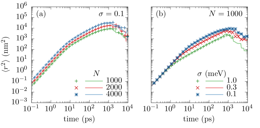
Figure 7: Mean square displacement of the exciton over time in the context of possible spin-flipping Förster transfer, as detailed in Appendix B. Solid lines denote scenarios without exciton FSS, while points represent results with non-zero FFS, specifically $0.1$ meV in each case. Panel (a) presents data for varying system sizes with a fixed disorder of $\sigma=0.1$ meV. In panel (b), data are depicted for different strengths of the disorder with a constant number of quantum dots, $N=1000$. The number of disorder realizations for each dataset is consistent at $N_{\mathrm{rep}}=150$.

The model used for the description of the diffusion within this work possesses some simplifications. In particular, it was assumed that the exciton is created via circularly polarized light, which forms a coherent superposition of the two possible bright excitions in a self-assembled quantum dot. One with spin projection $j_{z}=1$ and the other with $j_{z}=-1$. One exciton is $\ket{\mathrm{e},\mathrm{hh}}=\ket{\uparrow,\Downarrow}$ and the other is $\ket{\downarrow,\Uparrow}$. As investigated in [13] the Förster transfer differentiates between the two excions, i.e., it is possible to have spin-preserving and spin-flipping transfer with different magnitude. In addition, on-site exciton fine-structure splitting (FSS) can disturb the diffusion process, leading to Rabi oscillations within each QD. In this Appendix, we present and extend the model, which takes into account excitons FSS and two types of Förster transport — spin preserving and spin flipping. The derivation of such a model is straightforward from [7, 8], where we account for the dipole operator separately for each exciton, that is, $\bm{\hat{d}}_{\alpha}^{+}=\bm{d}_{0}^{+}(\outerproduct{+}{0})_{\alpha}+\mathrm{H.c.}$ and $\bm{\hat{d}}_{\alpha}^{-}=\bm{d}_{0}^{-}(\outerproduct{-}{0})_{\alpha}+\mathrm{H.c.}$ As substituted for Eq. 4 and following the steps of the derivation of the equation of motion, one obtains the spin-preserving Förster couplings $V_{\alpha\beta}^{aa}=-\hbar\Gamma_{0}G(k_{0}r_{\alpha\beta})$ identical to Eq. (8) and spin-flipping ones $V_{\alpha\beta}^{a\bar{a}}=-\hbar\Gamma_{0}G^{a\bar{a}}(k_{0}r_{\alpha\beta})$ with

$$G^{a\bar{a}}(x)=\frac{3}{8}e^{2i\varphi a}\left[\frac{\cos x}{x}-3\left(\frac{\sin x}{x^{2}}+\frac{\cos x}{x^{3}}\right)\right],$$ (44)

where the geometrical phase is attained. The index $a=\pm$ corresponds to the exciton polarization and $\bar{a}$ denotes the orthogonal polarization to $a$. Similarly, the elements of the dissipator matrix for the spin-preserving coupling are $\Gamma_{\alpha\beta}^{aa}=\Gamma_{0}F^{aa}(k_{0}r_{\alpha\beta})$, where $F^{aa}(x)\equiv F(x)$ defined in Eq. (10), while for spin flip transitions $\Gamma_{\alpha\beta}^{a\bar{a}}=\Gamma_{0}F^{a\bar{a}}\left(k_{0}r_{\alpha\beta}\right)$

$$F^{a\bar{a}}(x)=-\frac{3}{4}e^{2i\varphi a}\left[\frac{\sin x}{x}+3\left(\frac{\cos x}{x^{2}}-\frac{\sin x}{x^{3}}\right)\right].$$ (45)

Since the transfer depends on the absolute value of the Förster coupling, it should not depend on the geometrical phase $\varphi$. The mean square displacement of the exciton moving within the model presented is shown in Fig. 7 for some system sizes (a) and disorder strengths (b). The diffusion follows a three-step difusion as before. The saturation stage is poorly seen because of the finite exciton lifetime. One can see points representing the data for non-zero FFS follow lines, which correspond to the lack of the FSS. This suggest the FSS barely affects the diffusion.

References

- Mirkovic et al. [2016] T. Mirkovic, E. E. Ostroumov, J. M. Anna, R. van Grondelle, Govindjee, and G. D. Scholes, Chem. Rev. 117, 249 (2016).
- Ritz et al. [2002] T. Ritz, A. Damjanović, and K. Schulten, ChemPhysChem 3, 243 (2002).
- Kholmicheva et al. [2016] N. Kholmicheva, P. Moroz, H. Eckard, G. Jensen, and M. Zamkov, ACS Energy Lett. 2, 154 (2016).
- Santos et al. [2020] M. C. D. Santos, W. R. Algar, I. L. Medintz, and N. Hildebrandt, Trends Analyt Chem 125, 115819 (2020).
- Kułak et al. [2022] L. Kułak, A. Schlichtholz, and P. Bojarski, J. Phys. Chem. C 126, 11209 (2022), publisher: American Chemical Society.
- De Sales et al. [2004] F. V. De Sales, S. W. Da Silva, J. M. Cruz, A. F. Monte, M. A. Soler, P. C. Morais, M. J. Da Silva, and A. A. Quivy, Phys. Rev. B 70, 1 (2004).
- Kozub et al. [2012] M. Kozub, L. Pawicki, and P. Machnikowski, Phys. Rev. B 86, 121305 (2012).
- Miftasani and Machnikowski [2016] F. Miftasani and P. Machnikowski, Phys. Rev. B 93, 1 (2016).
- Cao et al. [2019] J. Cao, H. Zhang, X. Liu, N. Zhou, X. Pi, D. Li, and D. Yang, J. Phys. Chem. C 123, 23604 (2019).
- Förster [1948] T. Förster, Ann. Phys. 437, 55 (1948).
- Förster [1959] T. Förster, Discuss. Faraday Soc. 27, 7 (1959).
- Lehmberg [1970] R. H. Lehmberg, Phys. Rev. A 2, 883 (1970).
- Specht et al. [2015] J. F. Specht, A. Knorr, and M. Richter, Phys. Rev. B 91, 155313 (2015).
- Power and Zienau [1959] E. A. Power and S. Zienau, Philos. Trans. A Math. Phys. Eng. Sci. 251, 427 (1959).
- Woolley [1971] R. G. Woolley, Proc. R. Soc. Lond. 321, 557 (1971).
- Cohen-Tannoudji et al. [2008] C. Cohen-Tannoudji, J. DuPont-Roc, and G. Grynberg, Photons and atoms (Wiley-VCH Verlag, 2008).
- Stephen [1964] M. J. Stephen, J. Chem. Phys. 40, 669 (1964).
- Anderson [1958] P. W. Anderson, Phys. Rev. 109, 1492 (1958).
- Rodríguez et al. [2003] A. Rodríguez, V. A. Malyshev, G. Sierra, M. A. Martín-Delgado, J. Rodríguez-Laguna, and F. Domínguez-Adame, Phys. Rev. Lett. 90, 027404 (2003).
- Kawa and Machnikowski [2020] K. Kawa and P. Machnikowski, Phys. Rev. B 102, 174203 (2020).
- Breuer and Petruccione [2002] H.-P. Breuer and F. Petruccione, The theory of open quantum systems (Oxford University Press, London, England, 2002).
- Gardiner and Zoller [2010] C. W. Gardiner and P. Zoller, Quantum noise, Springer Series in Synergetics (Springer, Berlin, Germany, 2010).
- Kawa and Machnikowski [2022] K. Kawa and P. Machnikowski, Phys. Rev. B 105, 184204 (2022).
- Heyn et al. [2009] C. Heyn, A. Stemmann, T. Köppen, C. Strelow, T. Kipp, M. Grave, S. Mendach, and W. Hansen, Applied Physics Letters 94, 10.1063/1.3133338 (2009).
- Note [1] http://wcss.pl.