Numerical methods for stochastic simulations: application to contagion processes

Abstract

Approximate numerical methods are one of the most used strategies to extract information from many-interacting-agents systems. In particular, the binomial method is of extended use to deal with epidemic, ecological and biological models, since unbiased methods like the Gillespie algorithm can become unpractical due to high CPU time usage required. However, authors have criticized the use of this approximation and there is no clear consensus about whether unbiased methods or the binomial approach is the best option. In this work, we derive new scaling relations for the errors in the binomial method. This finding allow us to build rules to compute the optimal values of both the discretization time and number of realizations needed to compute averages with the binomial method with a target precision and minimum CPU-time usage. Furthermore, we also present another rule to discern whether the unbiased method or the binomial approach is more efficient. Ultimately, we will show that the choice of the method should depend on the desired precision for the estimation of averages.

I Introduction

Stochastic processes simulations are one of the main pillars of complexity science [1, 2, 3]. Indeed, the list of fruitful applications is endless and we can name but a few paradigmatic examples like the study of population dynamics in ecology [4, 5], gene expression [6], metabolism in cells [7], finances and market crashes [8, 9], epidemiology [10, 11, 12, 13], telecommunications [14], chemical reactions [15], quantum physics [16] and active matter [17]. As models become more intricate, there arises a technical challenge of producing stochastic trajectories in feasible computation times, since unbiased methods that generate unbiased realizations of stochastic trajectories may become unpractical due to lengthy computations. Approximate methods, such as the binomial approach in which we will focus, aim to solve this issue significantly by reducing CPU time usage. The use of the approximated methods is extended (see e.g. [18, 19, 20]), and some authors assert that they might be the only way to treat heterogeneous many agents systems effectively [21]. However, other works claim that the systematic errors induced by the approximations might not trade-off the reduction in computation time [22, 23]. The primary objective of this work is to shed light in this debate and assess in which circumstances the approximate binomial method can be advantageous with respect to the unbiased algorithms.

To solve this question, we derive a scaling relation for the errors of the binomial method. This result allows us to obtain optimal values for the discretization time and number of realizations to compute averages with a desired precision and minimum CPU time consumption. Furthermore, we derive a rule to discern if the binomial method is going to be faster than the unbiased counterparts. Lastly, we carried a numerical study to compare the performance of both the unbiased and binomial methods and check the applicability of our proposed rules.

Ultimately, we will show that the efficiency of the binomial method is superior to the unbiased approaches only when the target precision is below a certain threshold value.

II Two-state models

Although one can be more general, throughout this work we will focus on stochastic models of two-state agents, such that the possible states of the $i^{th}$ agent can be $\sigma_{i}=0$ or $\sigma_{i}=1$. Models of binary-state agents are widely used in many different applications, such as: proteins [24], $1/2$ spins [25], epidemic spreading [26, 10], voting dynamics [27], chemical reactions [28, 29], drug-dependence in pharmacology [30], etc. Spontaneous creation or annihilation of agents will not considered, therefore, its total number, $N$, is conserved. We furthermore assume Markovian dynamics, so given that the system is in a particular state at time $t$, the “microscopic rules” that dictate the switching between states just depend on the current state $\bm{\sigma}(t)=\left\{\sigma_{1}(t),\dots,\sigma_{N}(t)\right\}$. These microscopic rules are given in terms of the transition rates, defined as the conditional probabilities per unit of time to observe a transition,

$$w^{t}\left(\bm{\sigma}\rightarrow\bm{\sigma^{\prime}}\right):=\lim_{dt\rightarrow 0}\frac{P(\bm{\sigma^{\prime}};t+dt|\bm{\sigma};t)}{dt}.$$ (1)

A particular set of transitions in which we are specially interested define the “one-step processes”, meaning that the only transitions allowed are those involving the change of a single agent’s state, with rates

$$w^{t}_{i}(\sigma_{i}\to\sigma_{i}^{\prime}):=$$

$$w^{t}(\{\sigma_{1},\dots,\sigma_{i},\dots,\sigma_{N}\}\to\{\sigma_{1},\dots,\sigma_{i}^{\prime},\dots,\sigma_{N}\}),$$ (2)

for $i=1,\dots,N$. Our last premise is to consider only transition rates $w_{i}(\sigma_{i}\to\sigma_{i}^{\prime})$ that do not depend explicitly on time $t$. For binary-state systems, quite commonly, the rate of the process $\sigma_{i}=0\to\sigma_{i}=1$ is different of the reverse process $\sigma_{i}=1\to\sigma_{i}=0$ and we define the rate of agent $i$ as

$$w_{i}(\sigma_{i}) :=\begin{cases}w_{i}(0\to 1)\quad\text{ if }\sigma_{i}=0,\\ w_{i}(1\to 0)\quad\text{ if }\sigma_{i}=1.\end{cases}$$ (3)

Note that the rates could, in principle, be different for every agent and depend in an arbitrary way on the state of the system. The act of modelling is actually to postulate the functional form of these transition rates. This step is conceptually equivalent to the choice of a Hamiltonian in equilibrium statistical mechanics.

As a detailed observation is usually unfeasible, we might be interested on a macroscopic level of description focusing, for example, on the occupation number $n(t)$, defined as the total number of agents in state $1$,

$$n(t):=\sum_{i=1}^{N}\sigma_{i}(t),$$ (4)

being $N-n(t)$ the equivalent occupation of state $0$. In homogeneous systems, those in which $w_{i}(\sigma_{i})=w(\sigma_{i}),\,\forall i$, transition rates at this coarser level can be computed from those at the agent-level as

$$W(n\rightarrow n+1) =(N-n)w(0),$$

$$W(n\rightarrow n-1) =nw(1).$$ (5)

Some applications might require an intermediate level of description between the fully heterogeneous [Eq. II] and the fully homogeneous [Eq. (II)]. In order to deal with a coarse-grained heterogeneity, we define $\mathcal{C}$ different classes of agents. Agents can be labeled in order to identify their class, so that $l_{i}=\ell$ means that the $i^{th}$ agent belongs to the class labeled $\ell$ with $\ell\in[1,\mathcal{C}]$ and we require that all agents in the same class share the same transition rates $w_{i}(\sigma_{i})=w_{\ell}(\sigma_{i}),\,\forall l_{i}=\ell$. This classification allows us to define the occupation numbers $N_{\ell}$ and $n_{\ell}$ as the total number of agents of the $\ell^{th}$ class and the number of those in state $1$ respectively. Moreover, we can write the class-level rates:

$$W_{\ell}(n_{\ell}\rightarrow n_{\ell}+1) =\left(N_{\ell}-n_{\ell}\right)w_{\ell}(0),$$

$$W_{\ell}(n_{\ell}\rightarrow n_{\ell}-1) =n_{\ell}w_{\ell}(1).$$ (6)

In general, stochastic models are very difficult to be solved analytically. Hence, one needs to resort to numerical simulations than can provide suitable approximations to the quantities of interest. There are two main types of simulation strategies: unbiased continuous-time and discrete-time algorithms. Each one comes with its own advantages and disadvantages that we summarize in the next sections.

III Unbiased continuous-time algorithms

We proceed to summarize the main ideas behind the unbiased continuous-time algorithms, and refer the reader to  [31, 21, 32, 26, 33, 34] for a detailed description. Say that we know the state of the system $\bm{\sigma}(t)$ at a given time $t$. Such state will remain unchanged until a random time ${t^{\prime}}>t$, when the system experiences a transition or “jump” to a new state, also random, $\bm{\sigma}^{\prime}(t^{\prime})$:

$$\bm{\sigma}(t)\xrightarrow{{t^{\prime}}-t}\bm{\sigma^{\prime}}({t^{\prime}}).$$ (7)

Therefore, the characterization of a change in the system necessarily requires us to sample both the transition time $\Delta{t}={t^{\prime}}-t$ and the new state $\bm{\sigma^{\prime}}({t^{\prime}})$.

For one-step processes, new states are generated by changes in single agents $\sigma_{i}\to 1-\sigma_{i}$. The probability that agent $i$ changes its state in a time interval ${t^{\prime}}\in[t,t+dt]$ is $w_{i}\left(\sigma_{i}\right)dt$ by definition of transition rate. Therefore, the probability that the agent will not experience such transition in an infinitesimal time interval is $1-w_{i}\left(\sigma_{i}\right)dt$. Concatenating such infinitesimal probabilities, we can compute the probability $Q_{i}(\sigma_{i},\Delta t)$ that a given agent does not change its state during an arbitrary time lapse $\Delta t$ as well as the complementary probability $P_{i}(\sigma_{i},\Delta t)$ that it does change state as

$$Q_{i}(\sigma_{i},\Delta t)=\lim_{dt\rightarrow 0}(1-w_{i}(\sigma_{i})dt)^{\Delta t/dt}=e^{-w_{i}(\sigma_{i})\Delta t},$$

$$P_{i}(\sigma_{i},\Delta t)=1-e^{-w_{i}(\sigma_{i})\Delta t}.$$ (8)

Eq. (III) conforms the basic reasoning from which most of the continuous-time algorithms to simulate stochastic trajectories are built. It allows us to extend our basic postulate from Eq. (1), which only builds probabilities for infinitesimal times ($dt$), to probabilities of events of arbitrary duration ($\Delta t$). It is important to remark that Eq. (III) is actually a conditional probability: it is only valid provided that there are no other updates of the system in the interval $\Delta t$. From it we can also compute the probability density function that the $i^{th}$ agent remains at $\sigma_{i}$ for a non-infinitesimal time $\Delta t$ and then experiences a transition to $\sigma_{i}^{\prime}=1-\sigma_{i}$ in the time interval $[t+\Delta t,t+\Delta t+dt]$:

$$f_{i}(\sigma_{i};\Delta t)=e^{-w_{i}(\sigma_{i})\Delta t}w_{i}(\sigma_{i}).$$ (9)

The above quantity is also called first passage distribution for the $i^{th}$ agent. Therefore, given that the system is in state $\bm{\sigma}$ at time $t$, one can use the elements defined above to compute the probability that the next change of the system is due to a switching in the agent $i$ at time $t^{\prime}\in[t+\Delta t,t+\Delta t+dt]$:

$$\text{P($i^{th}$ agent switches state in $[t+\Delta t,t+\Delta t+dt]$) }\times$$

$$\text{P(Other agents change state only after $t+\Delta t+dt$) }=$$

$$f_{i}(\sigma_{i};\Delta t)dt\times\prod_{j\neq i}^{N}Q_{j}(\sigma_{j},\Delta t)=e^{-W(\bm{\sigma})\Delta t}w_{i}(\sigma_{i})dt,$$ (10)

where we have defined the total exit rate,

$$W(\bm{\sigma}):=\sum_{i=1}^{N}w_{i}(\sigma_{i}).$$ (11)

Two methods, namely the first-reaction method and Gillespie, can be distinguished based on the scheme used to sample the random jumping time ${t^{\prime}}$ and switching agent $i$ from the distribution specified in Eq. (III). The first-reaction method involves sampling one tentative random time per transition and choosing the minimum among them as the transition time that actually occurs. In contrast, the Gillespie algorithm directly samples the transition time and then determines which transition is being activated. See extended descriptions of these methods in [31, 21, 32, 35, 36].

IV Discrete-time approximations

In this section, we consider algorithms which at simulation step $s$ update time by a constant amount, $t_{s+1}=t_{s}+\Delta t$. Note that the discretization step $\Delta t$ is no longer stochastic, and it has to be considered as a new parameter that we are in principle free to choose. Larger values of $\Delta t$ result in faster simulations since fewer steps are needed in order to access enquired times. Nevertheless, the discrete-time algorithms introduce systematic errors that grow with $\Delta t$.

IV.1 Discrete-synchronous

It is possible to use synchronous versions of the process where all agents can potentially update their state at the same time $t_{s}$ using the probabilities $P_{i}(\sigma_{i},\Delta t)$ defined in Eq. (III) (see e.g. [34, 37]).

Algorithm 1 Discrete time synchronous agent level

1:Increment time: $t_{s+1}=t_{s}+\Delta t$

2:Compute all probabilities $P_{i}(\sigma_{i},\Delta t)$, $i=1,\dots,N$, using Eq. (III).

3:For all agents, generate a uniform random number $\hat{u}_{i}\in[0,1]$. If $\hat{u}_{i}<P_{i}(\sigma_{i},\Delta t)$ change the state $\sigma_{i}\to 1-\sigma_{i}$.

4:go to 1.

We note that the use of synchronous updates changes the nature of the process since simultaneous updates were not allowed in the original continuous-time algorithms. Given that the probabilities $P_{i}(\sigma_{i},\Delta t)$ tend to zero as $\Delta t\to 0$, one expects to recover the results of the continuous-time asynchronous approach in the limit $\Delta t\rightarrow 0$. Nevertheless, users of this method should bear in mind that this approximation could induce discrepancies with the continuous-time process that go beyond statistical errors [38].

IV.2 Binomial method: two simple examples

When building the class-version of the synchronous agent level (Algorithm 1), one can merge together events with the same transition probability and sample the updates using binomial distributions. This is the basic idea behind the binomial method, which is of extended use in the current literature (e.g. [39, 20, 40]). Since references presenting this method are scarce, we devote a longer section to its explanation.

Let us start with a simple example. Say that we are interested in simulating the decay of $N$ radioactive nuclei. We denote by $\sigma_{i}=1$ that nucleus $i$ is non-disintegrated and by $\sigma_{i}=0$ the disintegrated state. All nuclei have the same time-independent decay rate $\mu$:

$$w_{i}(1\rightarrow 0)=\mu,\quad w_{i}(0\rightarrow 1)=0.$$ (12)

This is, all nuclei can decay with the same probability $\mu dt$ in every time-bin of infinitesimal duration $dt$, but the reverse reaction is not allowed. This simple stochastic process leads to an exponential decay of the average number $n_{t}$ of active nuclei at time $t$ as $\langle n_{t}\rangle=Ne^{-\mu t}$.

Using the rates (12), we can compute the probability that one nucleus disintegrates in a non-infinitesimal time $\Delta t$ [Eq. III],

$$p:=P_{i}(1,\Delta t)=1-e^{-\mu\Delta t},\quad\forall i.$$ (13)

Therefore every particle follows a Bernoulli process in the time interval $\Delta t$. This is, each particle decays with a probability $p$ and remains in the same state with a probability $1-p$. So the total number of decays in a temporal-bin of duration $\Delta t$ follows a binomial distribution ${\bf B}(N,p)$,

$$P[n\text{ decays in {\hbox{\Delta t}}}]={N\choose n}p^{n}(1-p)^{N-n}.$$ (14)

The average of the binomial distribution is $\langle n\rangle=Np$ and its variance $\sigma^{2}[n]=Np(1-p)$. This result invites to draw stochastic trajectories with a recursive relation:

$$n_{t+\Delta t}=n_{t}-\Delta n_{t},$$ (15)

where we denote by $\Delta n_{t}\sim{\bf B}(n_{t},p)$ a random value drawn from the binomial distribution, with average value $\langle\Delta n_{t}\rangle=n_{t}p$, and we start from $n_{0}=N$. In this simple example, it turns out that Eq. (15) does generate unbiased realizations of the stochastic process. From this equation we obtain

$$\langle n_{t+\Delta t}\rangle_{B}=\langle n_{t}\rangle_{B}-\langle\Delta n_{t}\rangle_{B}=\langle n_{t}\rangle_{B}(1-p).$$ (16)

The symbol $\langle\cdot\rangle_{B}$ notes averages over the binomial method. The solution of this recursion relation with initial condition $n_{0}=N$ is

$$\langle n_{t}\rangle_{B}=N\left(1-p\right)^{\frac{t}{\Delta t}}=Ne^{-\mu t},$$ (17)

which coincides with the exact result independently of the value of $\Delta t$. Therefore, the choice of $\Delta t$ is just related to the desired time resolution of the trajectories. If $\Delta t\ll(N\mu)^{-1}$, many of the outcomes $\Delta n_{t}$ used in Eq. (15) will equal zero as the resolution would be much smaller than the mean time between disintegration events. Contrary, if $\Delta t\gg(N\mu)^{-1}$, much of the information about the transitions will be lost and we would generate a trajectory with abrupt transitions. Still, both simulations would faithfully inform about the state of the system at the enquired times [see Figs. 1 (a) and (b)].

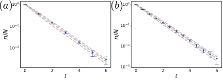
Figure 1: Simulations of the radioactive decay process with rates given by Eq.(12), using the binomial method [Eq. (15)]. In (a) the time discretization is $\Delta t=1$, whereas in (b) is $\Delta t=0.5$. In both panels $N=100$ and $\mu=1$. Dots and error bars indicate the average and standard error respectively, both computed from 20 simulations. With dashed lines, we show the analytical average (red) plus and minus the analytical standard error (gray): $\langle n(t)\rangle\pm\sigma[n(t)]/\sqrt{20}$. Independently of the discretization time, the results from simulations agree with the analytical value within errors.

Let us now apply this method to another process where it will no longer be exact. Nevertheless, the basic idea of the algorithm is the same: compute non-infinitesimal increments of stochastic trajectories using binomial distributions. In the so-called birth and death process, we consider a system with $N$ agents which can jump between states with homogeneous constant rates:

$$w_{i}(1\to 0)=\mu,\quad w_{i}(0\to 1)=\kappa.$$ (18)

Reasoning as before, the probabilities that a particle changes state in a non-infinitesimal time $\Delta t$ are:

$$P(0,\Delta t)=1-e^{-\kappa\Delta t},$$

$$P(1,\Delta t)=1-e^{-\mu\Delta t}.$$ (19)

Where we can avoid the use of subscripts since all agents share the transition rates. At this point, we might feel also invited to write an equation for the evolution of agents in state $1$ in terms of the stochastic number of transitions:

$$n_{t+\Delta t}=n_{t}-\Delta n_{t,1}+\Delta n_{t,0}.$$ (20)

Where $\Delta n_{t,1}$ and $\Delta n_{t,0}$ are binomial random variables distributed according to ${\bf B}(n_{t},P(1,\Delta t))$ and ${\bf B}(N-n_{t},P(0,\Delta t))$ respectively. However, trajectories generated with Eq. (20) turn out to be only an approximation to the original process. The reason is that the probability that a given number of transitions $0\rightarrow 1$ happen in a time window is modified as soon as a transition $1\rightarrow 0$ occurs (and vice-versa). If we now take averages in Eq. (20), use the known averages of the binomial distribution and solve the resulting linear iteration relation for $\langle n_{t}\rangle_{B}$, we obtain:

$$\langle n_{t}\rangle_{B}=\left(n_{0}-\frac{b}{a}\right)(1-a)^{t/\Delta t}+\frac{b}{a}$$ (21)

with $a=2-e^{-\mu\Delta t}-e^{-\kappa\Delta t}$ and $b=N(1-e^{-\kappa\Delta t})$. It is true that in the limit $\Delta t\to 0$, this solution recovers the exact solution for the evolution equation of the average number of non-disintegrated nuclei for the continuous-time process, namely

$$\frac{d\langle n_{t}\rangle}{dt} =-\mu\langle n_{t}\rangle+\kappa(N-\langle n_{t}\rangle),$$

$$\langle n_{t}\rangle =\left(n_{0}-N\frac{\kappa}{\kappa+\mu}\right)e^{-(\kappa+\mu)t}+N\frac{\kappa}{\kappa+\mu},$$ (22)

but the accuracy of the discrete approximation depends crucially on the value of $\Delta t$. If, for instance, we take $\Delta t\gg\max(\kappa^{-1},\mu^{-1})$, then we can approximate $a\approx 2$, $b\approx N$, such that Eq. (21) yields

$$\langle n_{t}\rangle_{B}=\begin{cases}N-n_{0},&\text{if}\ t/\Delta t\text{ odd},\\ n_{0},&\text{if}\ t/\Delta t\text{ even},\end{cases}$$ (23)

a numerical instability that shows up as a wild oscillation, see Fig. 2.

Therefore, the fact that agents are independent and rates are constant is not sufficient condition to guarantee that the binomial method generates unbiased trajectories for arbitrary values of the discretization step $\Delta t$. Nevertheless, it is remarkable that the only condition needed to ensure that Eq. (20) is a good approximation to the exact dynamics, Eq. (IV.2), is that $\Delta t\ll\min(\kappa^{-1},\mu^{-1})$. Given than the system size $N$ does not appear in this condition, we expect the binomial method to be very efficient to simulate this kind of process if we take a sufficiently small value for $\Delta t$, independently on the number of agents, see Fig. 2, where both $\Delta t=0.1,1$ produced a good agreement for $\mu=\kappa=1$. By comparing the average value of the binomial method, Eq.(21) with the exact value, Eq.(IV.2), we note that the error of the binomial approximation can be expanded in a Taylor series

$$\langle n_{t}\rangle_{B}-\langle n_{t}\rangle=\lambda\Delta t+\mathcal{O}(\Delta t^{2}).$$ (24)

where the coefficient of the linear term $\lambda$ depends on $t$ and $N$, as well as on other parameters of the model. We will check throughout this work that a similar expansion of the errors in the binomial method holds for the case of more complex models.

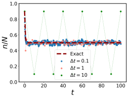
Figure 2: Three realizations of the birth and death process with constant rates defined by Eq. (18) simulated with the use of the binomial method [Eq. (20)]. In this case, we also use different time discretization $\Delta t$, and fixed $N=1000$, $\mu=1$, and $\kappa=1$. Note the numerical instability that shows up as wild oscillations in the numerical trajectories for the large time step $\Delta t=10$. Otherwise, there is a good agreement between simulations and the expected average value (dashed line) for both $\Delta t=0.1,1$

IV.3 Binomial method: general algorithm

If we go back to the general two-state process in which the functional form of the rates can have an arbitrary dependence on the state of the system, we can approximate the probability that the state of agent $i$ changes in $\Delta t$ by $P_{i}(\sigma_{i},\Delta t)$ [Eq. (III)]. If all these probabilities are different, we cannot group them in order to conform binomial samples. If, on the other hand, we can identify large enough classes such that all agents in each class have the same rates $w_{\ell}(\sigma)$, we can approximate the variation of the occupation number $n_{\ell}$ of each class during the time $\Delta t$ as the difference $\Delta n_{\ell,0}-\Delta n_{\ell,1}$ where $\Delta n_{\ell,0}$ and $\Delta n_{\ell,1}$ follow, respectively, binomial distributions $B(N_{\ell}-n_{\ell},P_{\ell}(0,\Delta t))$ and $B(n_{\ell},P_{\ell}(1,\Delta t))$, with $P_{\ell}(\sigma,\Delta t)$ given by Eq. (III) using any agent $i$ belonging to class $\ell$. All class occupation numbers are updated at the same time in step $s$, yielding the synchronous binomial algorithm, which reads:

Algorithm 2 Binomial synchronous class level

1:Update time as $t_{s+1}=t_{s}+\Delta t$.

2:For every class $\ell\in[1,\dots,\mathcal{C}]$:

3:   Update the values of $P_{\ell}(1,\Delta t),P_{\ell}(0,\Delta t)$, using Eq. (III).

4: Update the number of agents as $n_{\ell}\to n_{\ell}-\Delta n_{\ell,1}+\Delta n_{\ell,0}$, where $\Delta n_{\ell,1}$ and $\Delta n_{\ell,0}$ are values of binomial random variables distributed according to $B(n_{\ell},P_{\ell}(1,\Delta t))$ and $B(N_{\ell}-n_{\ell},P_{\ell}(0,\Delta t))$, respectively.

5:go to 1.

A similar reasoning could be built departing from the knowledge that the number of occurrences of continuous-time independent processes follows a Poisson distribution [15]. This conception gives rise to the tau-leaping algorithm [21, 26] used in the context of chemical modeling.

V The $\dfrac{27}{4}$ rule

The major drawback of the binomial method to simulate trajectories is the necessity of finding a proper discretization time $\Delta t$ that avoids both slow and inaccurate implementations. In this section, we propose a semi-empirical predictor for the values of the optimal choice of $\Delta t$ that propitiates the smallest computation time for a fixed desired accuracy. Moreover, we will present a rule to discern whether an unbiased continuous-time algorithm or the discrete-time binomial method is more suitable for the required task.

Consider that we are interested in computing the average value $\langle Z\rangle$ of a random variable $Z$ that depends on the stochastic trajectory in a time interval $[0,T]$. For example, $Z$ could be the number of nuclei for the process defined in Eq. (12) at a particular time $t\in[0,T]$. The standard approach to compute $\langle Z\rangle$ numerically generates $M$ independent realizations of the stochastic trajectories and measures the random variable $Z^{(i)}$ in each trajectory $i=1,\dots,M$. The average value $\langle Z\rangle$ is then approximated by the sample mean

$$Z_{M}:=\frac{1}{M}\sum_{i=1}^{M}Z^{(i)}.$$ (25)

Note that $Z_{M}$ itself should be considered a random variable as its value changes from a set of $M$ realizations to another.

For an unbiased method, such as Gillespie, the only error $\varepsilon$ in the estimation of $\langle Z\rangle$ by $Z_{M}$ is of statistical nature and can be computed from the standard deviation of $Z_{M}$, namely

$$\varepsilon=\frac{\sigma}{\sqrt{M}},\text{ with }\sigma:=\sqrt{\langle Z^{2}\rangle-\langle Z\rangle^{2}}.$$ (26)

The quantification of the importance of the error, for sufficiently large $M$, follows from the central limit theorem [41, 32] using the confidence intervals of a normal distribution:

$$P\left[\langle Z\rangle-\varepsilon\leq Z_{M}\leq\langle Z\rangle+\varepsilon\right]=0.6827\dots$$ (27)

It is in this sense, that one says that the standard error $\varepsilon$ is the precision of the estimation and writes accordingly

$$\langle Z\rangle=Z_{M}\pm\varepsilon.$$ (28)

Note that, according to Eq.(26), for an unbiased method the error in the estimation of the sample mean $Z_{M}$ tends to zero in the limit $M\to\infty$.

For a biased method, such as the binomial, that uses a finite discretization time $\Delta t$ and generates $M_{B}$ independent trajectories, the precision is altered by a factor that does not tend to zero in the limit $M_{B}\to\infty$. Based on the result found in the simple birth and death example of the previous section, let us assume for now that this factor scales linearly with the discretization time $\Delta t$ and can be written as $\lambda\Delta t$ where $\lambda$ is a constant depending on the model. We will corroborate this linear assumption both with calculations and numerical simulations in the next section. Then we can write the estimator using the binomial method as

$$\langle Z\rangle=Z_{M_{B}}+\lambda\Delta t\pm\varepsilon_{B},$$ (29)

where $\varepsilon_{B}=\dfrac{\sigma}{\sqrt{M_{B}}}$. The maximum absolute error of the biased method is then $|\lambda|\Delta t+\varepsilon_{B}$. Due to the presence of a bias term in the error, the only way that the precision of the binomial method can equal the one of an unbiased approach is by increasing the number of realizations $M_{B}$ compared to the number of realizations $M$ of the unbiased method. Matching the values of the errors of the unbiased and the biased methods and using $\varepsilon_{B}=\sqrt{\dfrac{M}{M_{B}}}\varepsilon$, we arrive at the condition that the required number of steps of the biased method is

$$M_{B}=M\left(\frac{|\lambda|\Delta t}{\varepsilon}-1\right)^{-2},$$ (30)

and the additional requirement $\Delta t\leq\frac{\varepsilon}{|\lambda|}$ (otherwise the bias is so large that it can not be compensated by the increase in the number of realizations $M_{B}$).

What a practitioner needs to know is the total CPU time $t_{B}^{\text{(CPU)}}$ the biased method needs to achieve the same accuracy $\varepsilon$ reached by the unbiased method. The CPU time to generate one stochastic trajectory is proportional to the number of steps, $\dfrac{T}{\Delta t}$, needed to reach the final time $T$ and can be written as $C_{B}\dfrac{T}{\Delta t}$, where $C_{B}$ is the CPU time needed to execute one iteration of the binomial method. Hence the total time required to generate $M_{B}$ trajectories is

$$t_{B}^{\text{(CPU)}}=C_{B}M_{B}\frac{T}{\Delta t}.$$ (31)

The discretization time associated with a minimum value of the CPU time consumption and subject to the constraint of fixed precision is obtained by inserting Eq. (30) in Eq. (31) and minimizing for $\Delta t$ (see Appendix A). The optimal time reads:

$$\Delta t^{\text{opt}}=\frac{1}{3}\frac{\varepsilon}{|\lambda|}.$$ (32)

Inserting the equation for the optimal $\Delta t$ in Eq. (30), one obtains:

$$M_{B}^{\text{opt}}=\frac{9}{4}M=\frac{9}{4}\left(\frac{\sigma}{\varepsilon}\right)^{2}.$$ (33)

Eqs. (32) and (33) have major practical use, since they tell us how to choose $\Delta t^{\text{opt}}$ and $M_{B}^{\text{opt}}$ to use the binomial method to reach the desired precision $\varepsilon$ and with minimum CPU time usage.

Still, one important question remains. Provided that we use the optimal pair ($M_{B}^{\text{opt}}$,$\Delta t^{\text{opt}}$), is the binomial method faster than an unbiased approach? In order to answer this question we first obtain the expected CPU time of the binomial method with the optimal choice inserting Eqs.(32) and (33) in Eq. (31):

$$t_{B}^{\text{(CPU,opt)}}=\frac{27}{4}\frac{C_{B}}{|\lambda|}\frac{\sigma^{2}}{\varepsilon}T.$$ (34)

On the other hand, the CPU time needed to generate one trajectory using the unbiased method is proportional to the maximum time $T$, and the total CPU time to generate $M$ trajectories is $t_{U}^{\text{(CPU)}}=CMT$, where $C$ is a constant depending of the unbiased method used. The expected ratio between the optimal CPU time consumption with the binomial method an the unbiased approach is

$$\alpha=\frac{t_{B}^{\text{(CPU,opt)}}}{t_{U}^{\text{(CPU)}}}=\frac{27}{4}\frac{C_{B}}{C}\frac{|\lambda|}{\varepsilon}.$$ (35)

Eq.(35) defines what we called “the $\frac{27}{4}$ rule”, and its usefulness lies in the ability to indicate in which situations the binomial method is more efficient than the unbiased procedure (when $\alpha<1$). Also from Eq.(35) we note that unbiased methods become the preferred option as the expected precision is increased, i.e. when $\varepsilon$ is reduced. We note that there is a threshold value $\varepsilon=\frac{27}{4}\frac{|\lambda|C_{B}}{C}$ for which both the unbiased and binomial methods are equally efficient.

Eqs. (32), (33) and (35) conform the main result of this work. These three equations (i) fix the free parameters of the binomial method ($\Delta t$ and $M_{B}$) in order to compute averages with fixed precision $\varepsilon$ at minimum CPU time usage, and (ii) inform us if the binomial method is more efficient than the unbiased method. The use of these equations require the estimation of four quantities: $\sigma$, $C$, $\lambda$, and $C_{B}$, which can be computed numerically with limited efforts. The standard deviation $\sigma$ depends only on the random variable $Z$ and has to be computed anyway in order to have a faithful estimate of the errors. As we will show in the examples of section VI, the constant $\lambda$ can be obtained through extrapolation at high values of $\Delta t$ (thus, very fast implementations). Finally, the constants $C$ and $C_{B}$ can be determined very accurately and at a little cost by measuring the CPU usage time of a few iterations with standard clock routines (both $C$ and $C_{B}$ depend as well on our ability to write efficient codes).

VI Numerical study

In this section, we want to compare the performance of the Gillespie algorithm (in representation of the unbiased strategies) and the binomial method. Also, we show the applicability of the rules derived in last section to fix the value of $\Delta t$ and decide whether the Gillespie or the binomial method is faster. We will do so in the context of the SIS model with both all-to-all connections and a meta-population structure.

VI.1 All-to-all

We study in this section the all-to-all connectivity, where every agent is connected to all others and have the same values of the transition rates. In the particular context of the SIS process, these rates read :

$$w(0\to 1)=\beta\sum_{j=1}^{N}\frac{\sigma_{j}}{N}=\beta\frac{n}{N},\quad w(1\to 0)=\mu.$$ (36)

Where $\mu$ represents the rate at which infected individuals recover from the disease and $\beta$ is the rate at which susceptible individuals catch the disease from an infected contact. The transition rates at the macroscopic description are also easily read from the macroscopic variable itself. From Eq. (II):

$$W(n\rightarrow n+1)=\beta\frac{n}{N}(N-n)$$

$$W(n\rightarrow n-1)=\mu n.$$ (37)

The main outcome of this all-to-all setting is well known and can easily be derived from the mean-field equation for the average number of infected [42],

$$\frac{d\langle n(t)\rangle}{dt}=\beta\frac{\langle n\rangle}{N}(N-\langle n\rangle)-\mu\langle n\rangle$$ (38)

and indicates that for $R_{0}\equiv\beta/\mu>1$ there is an “active” phase with a non-zero stable steady-sate value $\langle n\rangle_{\text{st}}=(1-\mu/\beta)N$, whereas for $R_{0}<1$ the stable state is the “epidemic-free” phase $\langle n\rangle_{\text{st}}=0$ where the number of infected individuals tends to zero with time.

In order to draw trajectories of this process with the binomial method we use Algorithm 2 with a single class containing all agents, $N_{\ell}=N,\,n_{\ell}=n$. The probability to use in the binomial distributions is extracted from the individual rates of Eq. (36):

$$P(1,\Delta t)=1-e^{-\mu\Delta t},\quad P(0,\Delta t)=1-e^{-\beta\frac{n}{N}\Delta t}.$$ (39)

We note that the probability $P(0,\Delta t)$ in Eq.(39) that a susceptible agent experiences a transition in a time $\Delta t$ is an approximation of

$$P(0,\Delta t)_{\text{exact}}=1-\exp{\left(-\frac{\beta}{N}\int_{t}^{t+\Delta t}n(s)ds\right)}.$$ (40)

Such approximation is a good representation of the original process when $\Delta t$ is so small that $n(t)$ can be considered as constant. In any case, we checked both analytically (see Appendix B) and numerically [see Fig. 3-(a) and (b)] that the errors of the method still scale linearly with the time discretization, as pointed out in section V.

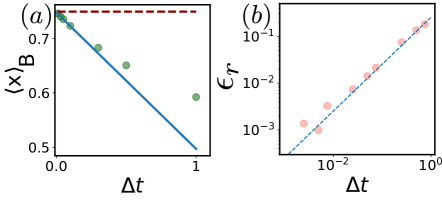
Figure 3: Panel (a) plots the average density $\langle x_{t}\rangle_{B}:=\dfrac{\langle n_{t}\rangle_{B}}{N}$ of infected individuals of the all-to-all SIS model at time $t=20$ obtained using the binomial method for different values of the discretization step $\Delta t$. The number of realizations is $M_{B}=100$, and other parameter values are $\beta=4$, $\mu=1$, $N=10^{3}$, $n(t=0)=10$. The statistical error bars are smaller than the symbol size. In accordance with Eq.(25), we find that there is a linear dependence at small $\Delta t$ with slope $\lambda=-0.25(1)$. The horizontal dashed line is the extrapolation at $\Delta t=0$ obtained from the linear fit. In panel (b) we plot for the same case, the relative error $\epsilon_{r}:=\left|\dfrac{\langle n_{t}\rangle_{B}}{\langle n_{t}\rangle}-1\right|$, using a very accurate value of $\dfrac{\langle n_{t}\rangle}{N}=0.7497$ obtained with the the so-called Gaussian approximation [43] , corroborating the linear dependence with the discretization step (dashed line of slope $1$).

Now let us discuss the crucial step of choosing the discretization $\Delta t$ of the binomial method. First we look for a condition on $\Delta t$ that ensures that Eq. (40) can be properly approximated by Eq. (39). Since the average time between updates at the non-zero fixed point is $W(n_{st})^{-1}=[(1-\mu/\beta)N/2]^{-1}$, a heuristic sufficient condition to ensure proper integration is to fix $\Delta t\propto 1/N$. In Fig. 4-(a), it is shown that this sufficient condition indeed generates a precise integration of the process. Also in Fig. 4-(a) we can see that this is in contrast with the use of $\Delta t=1$, which provides a poor representation of the process (as claimed in [22]). However, regarding the CPU-time consumption, the sufficient option performs poorly [Fig. 4-(b)]. Therefore, a proper balance between precision and CPU time consumption requires to fine tune the parameter $\Delta t$. This situation highlights the relevance of the rule derived in section V to choose $\Delta t$ and discern if the binomial method is advantageous with respect to the unbiased counterparts.

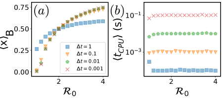
Figure 4: We plot in panel (a) the average density $\langle x_{t}\rangle_{B}:=\dfrac{\langle n_{t}\rangle_{B}}{N}$ of infected individuals of the all-to-all SIS model at time $t=20$ obtained using the binomial method as a function of $\mathcal{R}_{0}=\beta/\mu$ for different discretization times $\Delta t$. We take $n(t=0)=10$, $\mu=1.0$, $N=10^{3}$, and $M_{B}=100$. Statistical error bars are smaller than the symbol size. The estimations of the average agree within errors for $\Delta t=10^{-3}$ and $\Delta t=10^{-2}$. However, discrepancies are found for bigger values of $\Delta t$, for which the systematic errors are bigger than the statistical errors. Thus, the analysis of systematic errors should be taken into account to produce results with fixed desired precision . In panel (b), we plot the average CPU time (in seconds) per realization which, according to Eq.(31) scales as $1/\Delta t$. This plot evidences the need of a fine tuning of $\Delta t$ in order to avoid slow and imprecise calculations. It is relevant for the application of the $\frac{27}{4}$ rule that CPU time consumption (and therefore $C_{B}$) is not highly dependent on $\mathcal{R}_{0}$.

In Fig. 5-(a), we show the agreement of Eq. (35) with results from simulations. In this figure, the discretization step $\Delta t$ and number of realizations for the binomial method $M_{B}$ have been optimally chosen according to Eqs. (32) and (33). This figure informs us that the binomial method is more efficient than an unbiased Gillespie algorithm counterpart when the target error is large, namely for $\varepsilon\gtrsim 3\cdot 10^{-3}$, whereas the unbiased method should be the preferred choice for dealing with high precision estimators. In Fig. 5-(b) we fix the precision in the regime where the binomial method is more efficient and plot the CPU time consumption for both the binomial and Gillespie methods for different values of the transmission rate $\beta$. In this way, we can see explicitly the advantage of using the binomial method for low precision. In any case, the magnitude of the computation times is small for both methods and therefore we assess that the efficiency study is not needed for the case of all-to-all implementations. This situation is different for the case of more complex models, as the one treated in next section, for which approximate methods are needed to produce simulations in feasible times.

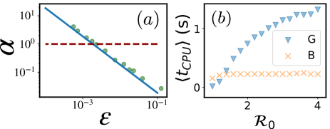
Figure 5: We plot in panel (a) the ratio between the CPU times of the binomial and the Gillespie algorithms applied to the simulation of an all-to-all SIS model with parameter values $T=20$, $\mu=1$, $\beta=2$, $N=10^{3}$, and $n(t=0)=10$ as a function of the target error $\varepsilon$. The dots are the results of the numerical simulations using for the binomial method the optimal values of the discretization step $\Delta t$ and number of realizations $M_{B}$ as given by Eqs. (32) and (33), while the number of trajectories in the Gillespie algorithm was computed from Eq. (26). The solid line is Eq. (35), using the values obtained from the simulations: $\sigma=0.031$, $\lambda=-0.25$, $C=4.45\cdot 10^{-3}$ s, $C_{B}=7.727\cdot 10^{-6}$ s. The dashed horizontal line at $\alpha=1$ signals where the Gillespie and binomial methods are equally efficient and it crosses the data at $\varepsilon=\frac{27}{4}\frac{|\lambda|C_{B}}{C}=3\cdot 10^{-3}$. In panel (b) we fix the precision $\varepsilon=0.01$, and plot the CPU-time to generate the ensemble of trajectories for different values of $\mathcal{R}_{0}=\frac{\beta}{\mu}$ for both the binomial (B) and the Gillespie (G) methods. Same parameter values $T$, $\mu$ and $N$ as in panel (a). $M$ and $M_{b}$ are computed as in (a). Except for $\mathcal{R}_{0}\lesssim 1$, where they perform similarly, the binomial method takes always less time than the Gillespie algorithm.

VI.2 Meta-population

The meta-population framework consist on $\mathcal{C}$ sub-systems, each of them containing a population of $N_{\ell}$ individuals, $\ell=1,\dots,\mathcal{C}$. Agents of different sub-populations are not connected and therefore cannot interact, whereas agents within the same population interact through an all-to-all scheme as defined in Sec. VI.1. Individuals can diffuse through populations, thus infected individuals can move to foreign populations and susceptible individuals can catch the disease abroad. Diffusion is tuned by a mobility matrix m, being the element $m_{\ell,\ell^{\prime}}$ the rate at which individuals from population $\ell$ travel to population $\ell^{\prime}$. Therefore, to fully specify the state of agent $i$ we need to give its state $\sigma_{i}$ and the sub-population $\ell_{i}$ it belongs to at a given time. Regarding the macroscopic description of the system, the inhabitants of a population can fluctuate and therefore it is needed to keep track of all the numbers $N_{\ell}$ as well as the occupation numbers $n_{\ell}$. The rates of all processes at the sub-population level are:

$$W_{\ell}(n_{\ell}\rightarrow n_{\ell}+1)=\beta\frac{n_{\ell}}{N_{\ell}}(N_{\ell}-n_{\ell}),$$

$$W_{\ell}(n_{\ell}\rightarrow n_{\ell}-1)=\mu n_{\ell},$$

$$W((N_{\ell},N_{\ell^{\prime}})\rightarrow(N_{\ell}-1,N_{\ell^{\prime}}+1))=m_{\ell,\ell^{\prime}}N_{\ell}.$$ (41)

If we assume homogeneous diffusion, the elements of the mobility matrix are $m_{\ell,\ell^{\prime}}=m$ if there is a connection between subpopulations $\ell$ and $\ell^{\prime}$ and $m_{\ell,\ell^{\prime}}=0$ otherwise. Also if the initial population distribution is homogeneous, $N_{\ell}(t=0)=N_{0},\,\forall\ell$, then the exit rate reads:

$$W(\bm{\sigma})=\sum_{\ell=1}^{\mathcal{C}}\left(\beta\frac{N_{\ell}-n_{\ell}}{N_{\ell}}+\mu\right)n_{\ell}+m\mathcal{C}N_{0},$$ (42)

which can be expressed as a function of the occupation variables $\{n_{\ell},N_{\ell}\}$. In this case, the average time between mobility-events, $[m\mathcal{C}N_{0}]^{-1}$, is constant and inversely proportional to the total number of agents $\mathcal{C}N_{0}$. This makes simulating meta-population models with unbiased methods computationally expensive, as a significant portion of CPU time is devoted to simulating mobility events and those methods are often infeasible. The binomial method is, therefore, the preferred strategy to deal with this kind of process [See Appendix C for details on how to apply the binomial method to meta-population models [44]]. However, one has to bear in mind that the proper use of the binomial method requires supervising the proper value of $\Delta t$ that generates a faithful description of the process at affordable times.

In Fig. 6-(a) we also check the applicability of the rules derived in section V, this time in the context of metapopulation models. As in the case of all-to-all interactions, the preferential use of the binomial method is conditioned to the desired precision for the estimator. Indeed, unbiased methods become more convenient as the target errors decrease. Also we show in the figure the remarkable similarity between the values of $\alpha$ [Eq. (35)] for the all-to-all and meta-population interactions. This result suggests that one can make the comparisons of efficiency suggested in section V using simple all-to-all models and then use the optimal values for $\Delta t$ and $M_{B}$ in complex meta-population structures. In Fig. 6-(b), the advantage of using the binomial method for low precision is explicitly shown. Compared to the case of the all-to-all interactions of section VI.1, the required CPU-time of the Gillespie method is very large, making it computationally very expensive to use. Therefore, this situation exemplifies the superiority of the binomial method with optimal choices for the discretization times and number of realizations, as derived in this work.

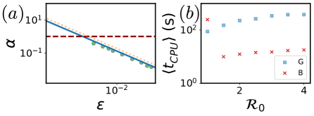
Figure 6: Panel (a): Similar to Fig.5 for the case of the meta-population SIS model with parameter values $t=5$, $\mu=1$, $\beta=2$. There are ${\cal C}=100$ subpopulations arranged in a square $10\times 10$ lattice such that each subpopulation is connected to $4$ nearest neighbors (we assume periodic boundary conditions); each subpopulation contains initially $N_{\ell}(t=0)=10^{3}$ agents, $\forall\ell$, and we have set the mobility amongst neighboring subpopulations to a constant value $m=10$. The discretization step and the number of trajectories of the binomial method take the optimal values of Eqs. (32) and (33), while the number of trajectories in the Gillespie algorithm was computed from Eq. (26). The required constants measured from the simulations are $\sigma=0.433$, $\lambda=-0.18$, $C=0.056$ s, $C_{B}=6.0\cdot 10^{-5}$ s. The dashed horizontal line at $\alpha=1$ signals where the Gillespie and binomial methods are equally efficient and it crosses the data at $\varepsilon=\frac{27}{4}\frac{|\lambda|C_{B}}{C}=1.3\cdot 10^{-3}$. The continuous line is the theoretical prediction Eq.(35), while the dotted line is the equivalent result obtained in the all-to-all version of the model. We note that the values of $\alpha$ for both the all-to-all and the meta-population structure are of similar magnitude. In (b) we set a target precision $\varepsilon=0.1$ and vary $\beta$ in order to get the desired $\mathcal{R}_{0}=\frac{\beta}{\mu}$. Except for very small $\mathcal{R}_{0}$, the binomial method is more efficient for this level of precision, taking about two orders of magnitude less time.

VII Discussion

This work provides a solution for the existing debate regarding the use of the binomial approximation to sample stochastic trajectories. The discretization time of the binomial method needs to be chosen carefully since large values can result in errors beyond the desired precision, while low values can produce extremely inefficient simulations. A proper balance between precision and CPU time consumption is necessary to fully exploit the potential of this approximation and make it useful.

We have demonstrated, through both numerical and analytical evidence, that the systematic errors of the binomial method scale linearly with the discretization time. Using this result, we can establish a rule for selecting the optimal discretization time and number of simulations required to estimate averages with a fixed precision while minimizing CPU time consumption. Furthermore, we derived another rule that can tell us in which cases the binomial method is superior to unbiased algorithms. In general, the advantage of using the binomial method depends on the target precision: the use of unbiased methods becomes more optimal as the target precision increases.

The numerical study of our proposed rules signals that the ratio of CPU times between the unbiased and binomial methods are similar in both all-to-all and meta-population structures. This result facilitates the use of the rules in the latter case. Indeed, one can develop the study of efficiency in the all-to-all framework and then use the optimal values of the discretization time and number of realizations in the more complex case of meta-populations.

Appendix A Optimal time

In this section, we show the proof for Eq. (32). Inserting Eqs. (26) and (30) in Eq. (31) we obtain:

$$t_{B}^{\text{(CPU)}}=\frac{MC_{B}T}{\Delta t}\left(\frac{|\lambda|\Delta t}{\varepsilon}-1\right)^{-2}.$$ (43)

The above equation informs about the CPU time consumption using the binomial method with a time discretization $\Delta t$. Eq.(43) has only one relative minimum for $\Delta t$ in the interval $[0,\frac{\varepsilon}{\lambda}]$:

$$\Delta t=\frac{1}{3}\frac{\varepsilon}{|\lambda|},$$ (44)

which we identify as the optimal choice for the time discretization.

Appendix B Scaling of errors with $\Delta t$

Consider a SIS model with all-to-all interactions, and let $n(t)$ be the number of infected individuals at time $t$. The probability that a susceptible agent will change its state at time $t^{\prime}\in[t,t+dt]$ is:

$$P(0,\Delta t)_{\text{exact}}=1-\exp{\left(-\frac{\beta}{N}\int_{t}^{t+\Delta t}n(s)ds\right)}.$$ (45)

In the context of the binomial approximation, this probability is approximated by:

$$P(0,\Delta t)=1-\exp{\left(-\frac{\beta}{N}n(t)\Delta t\right)}.$$ (46)

The difference between Eqs. (45) and (46) is the error associated to the use of Eq. (46) instead of Eq.(45). We call this difference $\Delta P$.

$$\Delta P=P(0,\Delta t)_{\text{exact}}-P(0,\Delta t)=\exp{\left(-\frac{\beta}{N}n(t)\Delta t\right)}-\exp{\left(-\frac{\beta}{N}\int_{t}^{t+\Delta t}n(s)ds\right)}.$$ (47)

Considering $\Delta t$ small, we can approximate

$$\int_{t}^{t+\Delta t}n(s)ds\approx n(t)\Delta t+n^{\prime}(t)\frac{\Delta t^{2}}{2}.$$ (48)

Where $n^{\prime}(t)=\frac{d}{dt}n(t)$. Inserting the above expression in Eq. (47), we obtain

$$\Delta P = \exp{\left(-\frac{\beta}{N}n(t)\Delta t\right)}-\exp{\left(-\frac{\beta}{N}\left[n(t)\Delta t+n^{\prime}(t)\frac{\Delta t^{2}}{2}\right]\right)}$$ (49)

$$= \exp{\left(-\frac{\beta}{N}n(t)\Delta t\right)}\left[1-\exp{\left(-\frac{\beta}{N}n^{\prime}(t)\frac{\Delta t^{2}}{2}\right)}\right]\approx\frac{\beta n^{\prime}(t)}{2N}\Delta t^{2}.$$

If we make use of the binomial method, the faithful increment in the number of infected individuals should be $\Delta n_{\text{exact}}$, a random variable drawn from a binomial distribution ${\bf B}\left(n(t),P(0,\Delta t)_{\text{exact}}\right)$. Instead, we use a random variable $\Delta n$ drawn from the approximate distribution ${\bf B}\left(n(t),P(0,\Delta t)\right)$. The difference between the mean values of the exact random variable and the actual one used in the numerical method is

$$\langle\Delta n\rangle_{\text{exact}}-\langle\Delta n\rangle=n(t)\Delta P\sim\Delta t^{2}.$$ (50)

Therefore, if we want to reach a final simulation time $T$, the accumulated error of using the approximation Eq. (47) for a number of iterations proportional to $T/\Delta t$ scales as $\Delta P/\Delta t\sim\Delta t$. This scaling is corroborated numerically in Fig. 3 of the main text.

Appendix C Binomial method on meta-population framework

In this section, we show how to adapt the binomial method (algorithm 2) to the case of meta-population models (described in section VI.2). Let $s_{\ell}(t)$ and $n_{\ell}(t)$ be, respectively, the number of susceptible and infected individuals in subpopulation $\ell=1,\dots,\mathcal{C}$ at time $t$. These occupation numbers fully characterize the state of the system. Note that the total number of agents in class $\ell$ at time $t$ is $N_{\ell}(t)=s_{\ell}(t)+n_{\ell}(t)$. We partition mobility and epidemic events and perform separate updates for each of them to sample the future state $\{s_{\ell}(t+\Delta t),n_{\ell}(t+\Delta t)\}_{\ell=1,\dots,\mathcal{C}}$.

-Mobility: The first step involves the calculation, for all sub-populations, of the number of agents who move within a time interval $\Delta t$. These quantities, denoted by $\{\Delta s_{\ell},\Delta n_{\ell}\}_{\ell=1,\dots,\mathcal{C}}$, are extracted from binomial distributions $\Delta n_{\ell}\sim{\bf B}\left(n_{\ell}(t),p^{\text{out}}_{\ell}\right)$, $\Delta s_{\ell}\sim{\bf B}\left(s_{\ell}(t),p^{\text{out}}_{\ell}\right)$ with $p^{\text{out}}_{\ell}=1-e^{-\Delta t\sum_{j}m_{\ell,j}}$. Then, traveling agents have to be distributed among neighboring sub-populations. We call $\Delta s_{\ell,\ell^{\prime}},\Delta n_{\ell,\ell^{\prime}}$, respectively, the number of susceptible and infected individuals entering in sub-population $\ell^{\prime}$ coming from $\ell$. Those numbers are sampled, respectively, from the multinomial distributions, ${\bf M}(\Delta n_{\ell};{\{p_{\ell,\ell^{\prime}}\}_{\ell^{\prime}=1,\dots,\mathcal{C}}})$ and ${\bf M}(\Delta s_{\ell};{\{p_{\ell,\ell^{\prime}}\}_{\ell^{\prime}=1,\dots,\mathcal{C}}})$, with $p_{\ell,\ell^{\prime}}=\dfrac{m_{\ell,\ell^{\prime}}}{\sum_{j}m_{\ell,j}}$. The general multinomial distribution ${\bf M}(N;p_{1},\dots,p_{k})$ is defined by the probabilities

$$P(n_{1},\dots,n_{k})={N\choose{n_{1}\cdots n_{k}}}p_{1}^{n_{1}}\dots p_{k}^{n_{k}}.$$ (51)

One possible method for sampling numbers $\{n_{1},\dots,n_{k}\}$ from a multinomial distribution is by using an ordered sequence of binomial samples [45].

$$n_{i}\sim{\bf B}\left(N-\sum_{j<i}n_{j},\frac{p_{i}}{1-\sum_{j<i}p_{j}}\right),\quad i=1,\dots,k.$$ (52)

At this point, the state of the system is updated with the mobility events:

$$n_{\ell}(t) = n_{\ell}(t)+\sum_{j}\Delta n_{j,\ell},$$ (53)

$$s_{\ell}(t) = s_{\ell}(t)+\sum_{j}\Delta s_{j,\ell},$$ (54)

but time is not yet increased $t\to t+\Delta t$ as the changes due to epidemic dynamics still need to be accounted for.

-Epidemics: Once agents have been reallocated according to the mobility dynamics [Eqs. (53,54)], occupation numbers are updated following the transmission and recovery rules [Eq. (36)]. To do so, we extract two binomial numbers per sub-population:

$$\Delta n_{\ell,1}\sim{\bf B}\left(n_{\ell}(t),1-e^{-\mu\Delta t}\right),\quad\quad\Delta{n}_{\ell,0}\sim{\bf B}\left[s_{\ell}(t),1-\exp\left({-\beta\frac{n_{\ell}(t)}{n_{\ell}(t)+s_{\ell}(t)}\Delta t}\right)\right],$$ (55)

The new state of the system reads,

$$n_{\ell}(t+\Delta t)=n_{\ell}(t)+\Delta{n}_{\ell,0}-\Delta{n}_{\ell,1},$$

$$s_{\ell}(t+\Delta t)=s_{\ell}(t)-\Delta{n}_{\ell,0}+\Delta{n}_{\ell,1},$$ (56)

and time is now updated $t\to t+\Delta t$.