FedCBO: Reaching Group Consensus in Clustered Federated Learning through Consensus-based Optimization

Abstract.

Federated learning is an important framework in modern machine learning that seeks to integrate the training of learning models from multiple users, each user having their own local data set, in a way that is sensitive to data privacy and to communication loss constraints. In clustered federated learning, one assumes an additional unknown group structure among users, and the goal is to train models that are useful for each group, rather than simply training a single global model for all users. In this paper, we propose a novel solution to the problem of clustered federated learning that is inspired by ideas in consensus-based optimization (CBO). Our new CBO-type method is based on a system of interacting particles that is oblivious to group memberships. Our model is motivated by rigorous mathematical reasoning, including a mean field analysis describing the large number of particles limit of our particle system, as well as convergence guarantees for the simultaneous global optimization of general non-convex objective functions (corresponding to the loss functions of each cluster of users) in the mean-field regime. Experimental results demonstrate the efficacy of our FedCBO algorithm compared to other state-of-the-art methods and help validate our methodological and theoretical work.

1. Introduction

The wide use of internet of things (IoT) devices in various applications such as home automation, personal health monitoring, and vehicle-to-vehicle communications has led to the generation of vast amounts of data across a collective of users. However, concerns around data privacy and security, as well as limitations on communication costs and bandwidth, have made it challenging for an individual user to take advantage of this large amount of stored information. This has motivated the design and development of federated learning (FL) strategies, which aim at pooling information from learning models trained on local devices to build models without relying on the collection of local data [28, 19].

Standard FL approaches aim to learn one global model for all local clients/users [28, 23, 30, 21]. However, data heterogeneity, also known as non-i.i.d. data, naturally arises in FL applications since data are usually generated from users’ personal devices. Thus, it is expected that no single global model can perform well across all clients [34]. On the other hand, it is reasonable to expect that users with similar backgrounds are likely to make similar decisions and thus generate data following similar distributions. This paper studies one formulation of federated learning with non-i.i.d. data, namely Clustered Federated Learning (CFL)[34, 15, 33, 25, 26]. In CFL, users are partitioned into different clusters, and the objective is to train models for each cluster of users. These clusters may represent, for example, groups of users with preferences in different categories of movies and TV series. Our focus in this work is on the mathematical modeling and analysis of CFL methods and on exploring CFL’s effectiveness in improving the performance of FL when dealing with non-i.i.d. data. Specifically, we investigate how CFL can create personalized models for clusters of users with similar preferences. Our research is motivated by previous studies of CFL that have shown promising results in enhancing the performance of FL in the non-i.i.d. data setting.

To start making our set-up more precise, let us consider the clustered federated learning setting with one global server and $N$ different agents. We assume that each agent belongs to one of $K$ non-overlapping groups denoted by $S_{1}^{*},\dots,S_{K}^{*}$. We further assume that each agent belonging to group $S_{k}^{*}$ owns data points generated from distribution $\mathcal{D}_{k}$ that can be used for training its own learning models. Ideally, an agent would seek to communicate with other agents in its group to accelerate the training process of its own model. However, under data privacy constraints (see the discussions of privacy in Remark 4), i.e. an agent will not share its local data with global server and other agents, the underlying partition $S_{1}^{*},\dots,S_{K}^{*}$ is never revealed to the learning algorithm. Let $l(\theta;z):\Theta\rightarrow\mathbb{R}$ be the loss function associated with data point $z$, where $\Theta\subset\mathbb{R}^{d}$ is the parameter space for the learning models. Our goal is to minimize the population loss function

(1) $$L_{i}(\theta):=\mathbb{E}_{z\sim\mathcal{D}_{i}}[l(\theta;z)]$$

for all $i\in[K]$ simultaneously. In other words, the goal is to find minimizers $\theta_{i}^{*}$ for all loss functions

(2) $$\theta_{i}^{*}\in\operatorname*{arg\,min}_{\theta\in\Theta}L_{i}(\theta),\quad i\in[K].$$

A toy example illustrating the clustered federated learning framework is shown in Fig. 1.

Figure 1. Toy example of a clustered federated learning problem. Each mobile phone user has an underlying cluster identity, here represented by the colors orange and blue. We aim to identify the group memberships of users while simultaneously training models for every cluster by communicating model parameters with the cloud global server.

As suggested by the discussion above, the main difficulty in CFL comes from the fact that cluster identities of users are unknown. A CFL algorithm must then be able to induce clustering among users and simultaneously train models in a distributed setting without relying on local data collection. In order to propose an algorithm that accomplishes this, in this paper we abstract the CFL problem and formulate it mathematically borrowing ideas from consensus-based optimization (CBO) [6, 8, 36]. CBO is a family of global optimization methodologies based on systems of interacting particles that seek consensus around global minimizers of target objectives. Precisely, consider

$$\min_{\theta\in\mathbb{R}^{d}}\;L(\theta),$$

where the target function $L$, which may be non-convex, is a continuous function with a unique global minimizer $\theta^{*}$. For each $i\in[N]$, let $\theta^{i}\in\mathbb{R}^{d}$ represent the position of particle $i$ and consider the following system of equations

(3) $$d\theta^{i}_{t}=-\lambda(\theta_{t}^{i}-m_{t})dt+\sigma|\theta_{t}^{i}-m_{t}|dB_{t}^{i},\qquad\text{for $i=1,2,\dots,N$},$$

where the $\{B^{i}\}_{i}$ are independent Brownian motions and $m_{t}$ is a weighted average defined by

$$m_{t}:=\frac{\sum_{i=1}^{N}\theta_{t}^{i}\exp\big{(}-\alpha L(\theta_{t}^{i})\big{)}}{\sum_{i=1}^{N}\exp\big{(}-\alpha L(\theta_{t}^{i})\big{)}}.$$

One can alternatively consider other types of noise for (3) (see [8, 7]). For instance, one may substitute the diffusion term in (3) with a geometric component-wise Brownian motion as in [8]. This allows to improve the performance of the CBO algorithm by making some assumptions independent of the dimension $d$, and then useful for machine learning applications in high dimension. One can also adapt in a more general and anisotropic way the noise by using a covariance matrix defined similarly to $m_{t}$ as in [7], a method called Consensus Based Sampling (CBS) in optimization mode. Here we will stick to the basic CBO method for simplicity and refer the interested reader to [8, 7] for more details on other existing variants of CBO.

We notice that the term $\exp(-\alpha L(\theta))$ in the formula for $m_{t}$ is the Gibbs distribution corresponding to the objective function $L(\theta)$ and temperature $\frac{1}{\alpha}$. The motivation for assigning weights in this way comes from the Laplace principle [29, 10], which states that for any probability measure $\rho\in\mathcal{P}(\mathbb{R}^{d})$ compactly supported with $\theta^{*}\in\text{supp}(\rho)$ we have

$$\lim_{\alpha\rightarrow+\infty}\bigg{(}-\frac{1}{\alpha}\log\bigg{(}\int_{\mathbb{R}^{d}}\exp\big{(}-\alpha L(\theta)\big{)}d\rho(\theta)\bigg{)}\bigg{)}=L(\theta^{*}).$$

Hence, if $\theta^{*}$ is the unique minimizer of $L$, then the measure $\exp(-\alpha L(\theta))\rho(\theta)$, normalized by a constant factor, will assign most of its mass to a small neighborhood of $\theta^{*}$, and if $\alpha$ is large enough, this measure will approximate the Dirac delta distribution at $\theta^{*}$. Consequently, the weighted-average $m_{t}$, which is the empirical first moment of a normalized version of the measure $\exp(-\alpha L(\theta))\rho(\theta)$, is a reasonable target for particles to follow as in equation (3).

Although CBO can be easily adapted to the distributed setting when cluster identities are known (as one could simply run CBO on each cluster), it is not directly applicable to CFL if the goal is to propose dynamics that are oblivious to agents’ identities. Our problem is also different from standard multi-objective optimization, for which CBO has already been adapted; see [3, 4]. Indeed, in standard multi-objective optimization the goal is to find a point that is Pareto optimal for $K$ different target functions, whereas our goal is to find, simultaneously, $K$ global minimizers for $K$ different objective functions. On the other hand, the CBO approach is inherently gradient-free, so it is preferable when the objective function is not smooth enough or its derivative is expensive to evaluate. However, if communication costs are expensive as in real FL applications, one may consider introducing additional local gradient terms in the dynamics of each user so that training may continue even when there is no communication among users.

1.1. Contributions and related works

1.1.1. Contributions

Motivated by the discussion above, we propose a new CBO-inspired interacting particle system (see (4) below and the discussion right after) that is suited for the clustered federated learning setting. In our system, the evolution of each individual particle is completely determined by its own loss function, its own identity, and the locations of the other particles but no knowledge of their identities. More precisely, our main contributions can be summarized as follows:
(1) We introduce a novel CBO-type framework that enables the minimization of $K$ objective functions in a CFL setting without knowing the cluster identity of any of the particles. This is achieved by introducing a mechanism that secretly forces consensus among particles belonging to the same cluster. Moreover, we incorporate a gradient term in the particle dynamics, which dramatically reduces the number of communication rounds required for the CBO algorithm to achieve good performance.
(2) We provide rigorous theoretical justification for the proposed framework. In particular, we prove the well-posedness of the proposed particle system and its convergence toward a mean-field limit equation and study the consensus behavior of the mean-field dynamics and their ability to concentrate around global minimizers of each of the underlying loss functions.
(3) We discretize our continuous dynamics in a reasonable way and fit it into the conventional federated training protocol to obtain a new federated learning algorithm that we call FedCBO. We conduct extensive numerical experiments to verify the efficiency of our algorithm and demonstrate that it outperforms other state-of-the-art methods in the non-i.i.d. data setting.

1.1.2. Related work in clustered federated learning

In the setting of CFL, it is assumed that there is an underlying clustering structure among users, and the goal is to identify the clusters’ identities and federate among each group. Both IFCA [15] and HypCluster [27] alternate between identifying cluster identities of users and updating models for the user clusters via local gradient descent. These methods identify cluster identities by finding the model with the lowest loss on each local dataset. FedSEM [25] groups the users at each federated step by measuring the distance between users using model parameters and accuracy and then running a simple $K$-means algorithm. All these methods require prior knowledge or estimation of the number of underlying clusters, which may be difficult to have/do in practice. In contrast, as we discuss below, our method does not require any prior knowledge of the clustering structure, and consensus among clients in the same cluster will be automatically induced by our particle dynamics.

In [34], clusters are found in a hierarchical way. In particular, clients are recursively divided into two sets based on the cosine similarity of the clients’ model gradients or weight-updates. WeCFL [26] formalizes clustered federated learning problems into a unified bi-level optimization framework. Unlike the two framework mentioned above [34, 26], which conduct the convergence analysis under convexity assumptions, our paper considers target functions that are non-convex and provide an asymptotic convergence result in the mean-field regime.

1.1.3. Related work in consensus-based optimization

The idea of using interacting particle dynamics with consensus-inducing terms to solve global optimization problems was first introduced in [31]. Since then, this approach has gained a lot of interest from both theoretical and applied perspectives.

On the theoretical side, [6] provided the first local convergence analysis of a mean-field CBO equation under relatively stringent assumptions on the initialization of the system. This is achieved by first proving consensus formation at the mean-field level in the infinite time horizon and then tuning the consensus point using the Laplace principle. Later, [13] relaxed some of these stringent assumptions and proved that mean-field dynamics can reach an arbitrary level of concentration around a global minimizer within a finite time interval; however, this time horizon may be difficult to estimate a priori. By showing that the finite particle CBO system converges to the mean-field limit, [16] furthers the theoretical underpinnings of the CBO framework. In our paper, we use similar strategies as in [13, 32] and [16] to study the behavior of our mean field system (Section 4) and prove that our proposed particle dynamics converge toward a suitable mean-field limit (Section 5). In our setting, we need to face new challenges due to the fact that particles may have different dynamics that depend on the loss functions that they try to optimize. For instance, we need to estimate the time horizon needed to achieve a given accuracy at the mean field level differently from [13, 32]. Likewise, our convergence of the finite particle system toward a suitable mean field limit involves additional technical difficulties arising from the fact that in our setting there are multiple types of particles interacting with each other.

On the algorithmic side, with motivations from a variety of applications, researchers have extended and adapted the original CBO model to include new settings such as global optimization on compact manifolds like the sphere [12], general constraints [9], high-dimensional machine learning problems [8], global optimization of objective functions with multiple minimizers [5], sampling from distributions [7, 5], and saddle point optimization problems [17]. In [32], the authors introduce a gradient term in the CBO system which is shown to be beneficial numerically when applied the compressed sensing problems. In our paper, we also incorporate gradient information in our particle dynamics, but our motivation, different from the one in [32], is to reduce communication costs among users, one of the important practical constraints in federated learning. For a more comprehensive review of the development of CBO-type methods we refer the interested reader to the recent survey [36].

1.2. Notation

We use $|\cdot|$ to denote the absolute value or $\ell_{2}$-norm of vectors in Euclidean space and denote by $B_{r}(\theta)$ the open ball of radius $r$ centered at $\theta\in\mathbb{R}^{d}$. We denote by $\mathcal{C}(X,Y)$ the space of continuous functions $f:X\rightarrow Y$ between $X\subset\mathbb{R}^{n}$ and a given topological space $Y$. The space $\mathcal{C}(X,Y)$ is endowed with the sup-norm as is standard. When $Y=\mathbb{R}$, we simply use the notation $\mathcal{C}(X)$. We also use $\mathcal{C}_{c}^{k}(X)$ and $\mathcal{C}_{b}^{k}(X)$ to denote, respectively, the space of real-valued functions that are $k$-times continuously differentiable with compact support and the space of bounded functions that are $k$-times continuously differentiable. Let $\mathcal{P}(\mathbb{R}^{d})$ be the space of all Borel probability measures over $\mathbb{R}^{d}$ equipped with the Levy-Prokhorov metric, which metrizes the topology of weak convergence. For a given $p\geq 1$, we let $\mathcal{P}_{p}(\mathbb{R}^{d})\subseteq\mathcal{P}(\mathbb{R}^{d})$ be the collection of probability measures $\rho\in\mathcal{P}(\mathbb{R}^{d})$ with finite $p$-th moments, i.e., $\int_{\mathbb{R}^{d}}|\theta|^{p}d\rho(\theta)<\infty$. The space $\mathcal{P}_{p}(\mathbb{R}^{d})$ is endowed with the $p$-Wasserstein distance $W_{p}$ ($1\leq p<\infty$) defined according to

$$W_{p}(\rho,\hat{\rho}):=\inf_{\pi\in\Gamma(\rho,\hat{\rho})}\int_{\mathbb{R}^{d}\times\mathbb{R}^{d}}|\theta-\hat{\theta}|^{p}\pi(d\theta,d\hat{\theta}),\qquad\rho,\hat{\rho}\in\mathcal{P}_{p}(\mathbb{R}^{d}),$$

where $\Gamma(\rho,\hat{\rho})$ denotes the set of all joint probability measures over $\mathbb{R}^{d}\times\mathbb{R}^{d}$ with first and second marginals $\rho$ and $\hat{\rho}$, respectively.

When studying the laws of stochastic processes $\rho\in\mathcal{C}([0,T],\mathcal{P}(\mathbb{R}^{d}))$, we denote the law at time $t$ as $\rho_{t}\in\mathcal{P}(\mathbb{R}^{d})$. Given a continuous function $f\in\mathcal{C}(\mathbb{R}^{d})$ and a fixed probability measure $\rho\in\mathcal{P}(\mathbb{R}^{d})$, we denote by $\|f\|_{\mathbb{L}^{1}(\rho)}:=\int_{\mathbb{R}^{d}}|f(\theta)|d\rho(\theta)$ the $L^{1}$-norm of $f$ with respect to the measure $\rho$.

1.3. Organization of the paper

The rest of the paper is organized as follows. In Section 2.1, we introduce the interacting particle system motivating our FedCBO algorithm. In Section 2.2, we state our main theoretical results, which include the well-posedness of a mean-field system associated to our proposed interacting particle dynamics (Theorem 2.1), the convergence of the interacting particle system toward the mean-field as the number of particles in the system grows (Theorem 2.2)), and, finally, the behavior of the mean-field in time and its ability to concentrate around global optimizers for each of the objective functions (Theorem 2.3). Motivated by our particle system, in Section 2.3 we introduce our FedCBO algorithm. In Section 2.4, we present a series of numerical experiments to validate our proposed algorithm. Section 3 is devoted to the proof of Theorem 2.1, Section 4 to the proof of Theorem 2.3, and Section 5 to the proof of Theorem 2.2. We wrap up the paper in Section 6, where we summarize our contributions and discuss future research directions.

2. CBO for Clustered Federated Learning

2.1. Model formulation

In the rest of the paper we assume, without the loss of generality, that there are only two clusters in the CFL problem (2), i.e., $K=2$. Indeed, it will become clear from our discussion below that extending the proposed model and its corresponding theoretical analysis to the case $K>2$ is straightforward. We also assume that all agents in class $1$ use a single loss function $L_{1}$ and all agents in class $2$ use a single loss function $L_{2}$. In order to optimize $L_{1}$ and $L_{2}$ simultaneously, we consider a collection of $N\in\mathbb{N}$ interacting particles with positions {$\theta_{t}^{1,i}\}_{i=1}^{N_{1}}\in\mathbb{R}^{d}$ (class $1$ particles) and $\{\theta_{t}^{2,j}\}_{j=1}^{N_{2}}\in\mathbb{R}^{d}$ (class $2$ particles) described by the system of stochastic differential equations:

(4a) $$d\theta_{t}^{1,i}=-\lambda_{1}(\theta_{t}^{1,i}-m_{t}^{1})dt-\lambda_{2}\nabla L_{1}(\theta_{t}^{1,i})dt+\sigma_{1}|\theta_{t}^{1,i}-m_{t}^{1}|dB_{t}^{1,i}+\sigma_{2}|\nabla L_{1}(\theta_{t}^{1,i})|d\widetilde{B}_{t}^{1,i}$$

(4b) $$d\theta_{t}^{2,j}=-\lambda_{1}(\theta_{t}^{2,j}-m_{t}^{2})dt-\lambda_{2}\nabla L_{2}(\theta_{t}^{2,j})dt+\sigma_{1}|\theta_{t}^{2,j}-m_{t}^{2}|dB_{t}^{2,j}+\sigma_{2}|\nabla L_{2}(\theta_{t}^{2,i})|d\widetilde{B}_{t}^{2,j}$$

(4c) $$m_{t}^{1}:=\frac{\sum_{i=1}^{N_{1}}\theta_{t}^{1,i}w_{L_{1}}^{\alpha}(\theta_{t}^{1,i})+\sum_{j=1}^{N_{2}}\theta_{t}^{2,j}w_{L_{1}}^{\alpha}(\theta_{t}^{2,j})}{\sum_{i=1}^{N_{1}}w_{L_{1}}^{\alpha}(\theta_{t}^{1,i})+\sum_{j=1}^{N_{2}}w_{L_{1}}^{\alpha}(\theta_{t}^{2,j})}$$

(4d) $$m_{t}^{2}:=\frac{\sum_{i=1}^{N_{1}}\theta_{t}^{1,i}w_{L_{2}}^{\alpha}(\theta_{t}^{1,i})+\sum_{j=1}^{N_{2}}\theta_{t}^{2,j}w_{L_{2}}^{\alpha}(\theta_{t}^{2,j})}{\sum_{i=1}^{N_{1}}w_{L_{2}}^{\alpha}(\theta_{t}^{1,i})+\sum_{j=1}^{N_{2}}w_{L_{2}}^{\alpha}(\theta_{t}^{2,j})},$$

with $\lambda_{1},\lambda_{2},\sigma_{1},\sigma_{2}>0$, $w_{L_{k}}^{\alpha}(\theta):=\exp(-\alpha L_{k}(\theta))$ for $k=1,2$, and $\alpha>0$. In the sequel, we may use the terms particle and user interchangeably to refer to an agent.

Let us discuss the above system term by term. Equation (4a) describes the time evolution of the model parameters of agent $i$ in class $1$, while equation (4b) does the same for agent $j$ in class $2$. The term $m_{t}^{1}$ defined in (4c) is a weighted-average of all particle positions $\{\theta_{t}^{1,i}\}_{i=1}^{N_{1}},\{\theta_{t}^{2,j}\}_{j=1}^{N_{2}}$ with respect to the loss function $L_{1}$. In particular, an agent in class $1$ can compute $m_{t}^{1}$ without knowing the class identities of any of the other agents, an essential feature for our purposes. If we imagine for a moment that class $1$ particles concentrate around regions where $L_{1}$ is small, one should expect that $\{\theta_{t}^{1,i}\}_{i=1}^{N_{1}}$ have smaller $L_{1}$-loss than the class $2$ particles $\{\theta_{t}^{2,j}\}_{j=1}^{N_{2}}$, which presumably should concentrate around regions where the loss function $L_{2}$ is small. Then, intuitively, in the expression for $m_{t}^{1}$ class $1$ particles $\{\theta_{t}^{1,i}\}_{i=1}^{N_{1}}$ will receive higher weights than class $2$ particles and hence $m_{t}^{1}$ should be close to the weighted-average of the particles $\{\theta_{t}^{1,i}\}_{i=1}^{N_{1}}$ only. Thus, $m_{t}^{1}$ can be thought of as an evolving consensus point that corresponds to class $1$ particles only. A similar intuition holds for $m_{t}^{2}$, which is an evolving consensus point for class $2$ particles only. The first part of the drift terms in both (4a) and (4b) can then be thought of as a consensus-inducing term for each of the classes. The second part of the drift terms in (4a) and (4b), on the other hand, introduces local gradient information, which can be interpreted as a local model update through gradient descent. In federated learning, using local gradient information ensures that all models continue to update even when there is no communication between them; as discussed in [28], communication in federated settings is in general costly. Finally, the diffusion terms in the dynamics guarantee that each particle continues to explore the optimization landscape of its loss function until it reaches a critical point and aligns with its class consensus point. The $d$-dimensional Brownian motions $\{{B}^{k,i}\}_{k,i}$, $\{\widetilde{B}^{k,i}\}_{k,i}$ are assumed to be independent of each other.

Let us denote by $\bm{\theta}_{t}^{1,N}:=\{\theta_{t}^{1,1},\dots,\theta_{t}^{1,N_{1}}$}, $\bm{\theta}_{t}^{2,N}:=\{\theta_{t}^{2,1},\dots,\theta_{t}^{2,N_{2}}\}$ with $N=N_{1}+N_{2}\in\mathbb{N}$ the solution of the particle system (4). Consider its empirical measures given by

(5) $$\rho_{t}^{1,N}:=\frac{1}{N_{1}}\sum_{i=1}^{N_{1}}\delta_{\theta_{t}^{1,i}},\qquad\rho_{t}^{2,N}:=\frac{1}{N_{2}}\sum_{j=1}^{N_{2}}\delta_{\theta_{t}^{2,j}},\qquad\rho_{t}^{N}:=\frac{N_{1}}{N}\rho_{t}^{1,N}+\frac{N_{2}}{N}\rho_{t}^{2,N},$$

where we use $\delta_{\theta}$ to represent a Dirac delta measure at $\theta\in\mathbb{R}^{d}$. Observe that $m_{t}^{1},m_{t}^{2}$ can be rewritten in terms of $\rho_{t}^{N}$ as follows:

$$m_{t}^{1}=\frac{1}{\|w_{L_{1}}^{\alpha}\|_{\mathbb{L}^{1}(\rho_{t}^{N})}}\int\theta w_{L_{1}}^{\alpha}d\rho_{t}^{N}=:m_{L_{1}}^{\alpha}[\rho_{t}^{N}],\qquad m_{t}^{2}=\frac{1}{\|w_{L_{2}}^{\alpha}\|_{\mathbb{L}^{1}(\rho_{t}^{N})}}\int\theta w_{L_{2}}^{\alpha}d\rho_{t}^{N}=:m_{L_{2}}^{\alpha}[\rho_{t}^{N}].$$

In turn, system (4) can be rewritten as

$$d\theta_{t}^{1,i} =-\lambda_{1}(\theta_{t}^{1,i}-m_{L_{1}}^{\alpha}[\rho_{t}^{N}])dt-\lambda_{2}\nabla L_{1}(\theta_{t}^{1,i})+\sigma_{1}|\theta_{t}^{1,i}-m_{L_{1}}^{\alpha}[\rho_{t}^{N}]|dB_{t}^{1,i}+\sigma_{2}|\nabla L_{1}(\theta_{t}^{1,i})|d\widetilde{B}_{t}^{1,i},$$

$$d\theta_{t}^{2,j} =-\lambda_{1}(\theta_{t}^{2,j}-m_{L_{2}}^{\alpha}[\rho_{t}^{N}])dt-\lambda_{2}\nabla L_{2}(\theta_{t}^{2,j})+\sigma_{1}|\theta_{t}^{2,j}-m_{L_{2}}^{\alpha}[\rho_{t}^{N}]|dB_{t}^{2,j}+\sigma_{2}|\nabla L_{2}(\theta_{t}^{2,j})|d\widetilde{B}_{t}^{2,j}.$$

Based on the above expression, we can formally postulate a mean-field SDE system characterizing the time evolution of particles as $N_{1},N_{2}\rightarrow\infty$. Precisely, we consider the system of two SDEs:

(7a) $$d\overline{\theta}_{t}^{1}=-\lambda_{1}(\overline{\theta}_{t}^{1}-m_{L_{1}}^{\alpha}[\rho_{t}])dt-\lambda_{2}\nabla L_{1}(\overline{\theta}_{t}^{1})dt+\sigma_{1}|\overline{\theta}_{t}^{1}-m_{L_{1}}^{\alpha}[\rho_{t}]|dB_{t}^{1}+\sigma_{2}|\nabla L_{1}(\overline{\theta}_{t}^{1})|d\widetilde{B}_{t}^{1},$$

(7b) $$d\overline{\theta}_{t}^{2}=-\lambda_{1}(\overline{\theta}_{t}^{2}-m_{L_{2}}^{\alpha}[\rho_{t}])dt-\lambda_{2}\nabla L_{2}(\overline{\theta}_{t}^{2})dt+\sigma_{1}|\overline{\theta}_{t}^{2}-m_{L_{2}}^{\alpha}[\rho_{t}]|dB_{t}^{2}+\sigma_{2}|\nabla L_{2}(\overline{\theta}_{t}^{2})|d\widetilde{B}_{t}^{2},$$

where

$$m_{L_{k}}^{\alpha}[\rho_{t}]=\int\theta d\eta_{k,t}^{\alpha},\quad\eta_{k,t}^{\alpha}=w_{L_{k}}^{\alpha}\rho_{t}/\|w_{L_{k}}^{\alpha}\|_{\mathbb{L}^{1}(\rho_{t})},\quad\rho_{t}^{k}=Law(\overline{\theta}_{t}^{k}),\quad\rho_{t}=w_{1}\rho_{t}^{1}+w_{2}\rho_{t}^{2},$$

subject to the independent initial conditions $\overline{\theta}_{0}^{1}\sim\rho_{0}^{1}$ and $\overline{\theta}_{0}^{2}\sim\rho_{0}^{2}$; in the above, $B^{1},\widetilde{B}^{1},B^{2},\widetilde{B}^{2}$ are independent $d$-dimensional Brownian motions. Equations (7a) and (7b) describe, respectively, the effective time evolutions of individual particles of class $1$ and $2$ in the regime of a large number of particles. The weight $w_{k}$ represents the asymptotic proportion of particles of type $k$ in the system. Finally, $\rho_{t}^{1}$ and $\rho_{t}^{2}$ represent, respectively, the distributions of particles of class $1$ and $2$ at time $t$. Notice that the system (7) is coupled through the distribution $\rho_{t}$ of agents of both types. In Section 5, we discuss in precise mathematical terms the relationship between the finite system of interacting particles (4) and the mean-field limit system described in (7); see also Theorem 2.2 below.

The system of Fokker-Planck equations corresponding to (7) reads:

(8a) $$\partial_{t}\rho_{t}^{1} :=\Delta(\kappa_{t}^{1}\rho_{t}^{1})+\nabla\cdot(\mu_{t}^{1}\rho_{t}^{1}),\qquad\lim_{t\rightarrow 0}\rho_{t}^{1}=\rho_{0}^{1}$$

(8b) $$\partial_{t}\rho_{t}^{2} :=\Delta(\kappa_{t}^{2}\rho_{t}^{2})+\nabla\cdot(\mu_{t}^{2}\rho_{t}^{2}),\qquad\lim_{t\rightarrow 0}\rho_{t}^{2}=\rho_{0}^{2},$$

where

$$\mu_{t}^{k}:=\lambda_{1}(\theta-m_{L_{k}}^{\alpha}[\rho_{t}])+\lambda_{2}\nabla L_{k}(\theta),\quad\kappa_{t}^{k}:=\frac{\sigma_{1}^{2}}{2}|\theta-m_{L_{k}}^{\alpha}[\rho_{t}]|^{2}+\frac{\sigma_{2}^{2}}{2}|\nabla L_{k}(\theta)|^{2},\quad\text{for $k=1,2$.}$$

This is a non-linear system of equations that describes the time evolution of the distributions of agents of each class in the mean-field limit. Notice that we can indeed describe the law of the joint system of agents in the mean field limit just with the laws of the two marginals $\rho^{1}$ and $\rho^{2}$, thanks to the independence of the processes $\overline{\theta}^{1}$ and $\overline{\theta}^{2}$, which we discuss in Remark 7. In section 5.2, however, it will be more convenient to work with the law of the joint process $(\overline{\theta}^{1}_{t},\overline{\theta}^{2}_{t})$ explicitly. We do this to facilitate our study of the convergence of the finite particle system toward the mean-field. These details will be presented in due course.

In the sequel we interpret the Fokker-Planck system (8) in the weak sense.

Definition 2.1.

For $k=1,2$, let $\rho_{0}^{k}\in\mathcal{P}(\mathbb{R}^{d})$. Let $T>0$ be a given time horizon. We say that $\rho^{1},\rho^{2}\in\mathcal{C}([0,T],\mathcal{P}(\mathbb{R}^{d}))$ satisfy, in the weak sense, the Fokker-Planck equation (8) for the time interval $[0,T]$ and with initial conditions $(\rho_{0}^{1},\rho^{2}_{0})$ if for $\forall\phi\in\mathcal{C}_{c}^{\infty}(\mathbb{R}^{d})$, all $\forall t\in(0,T)$ and $k=1,2$, we have

$$\frac{d}{dt}\int\phi(\theta)d\rho_{t}^{k}(\theta)= \int\left(-\lambda_{1}(\theta-m_{L_{k}}^{\alpha}[\rho_{t}])-\lambda_{2}\nabla L_{k}(\theta)\right)\cdot\nabla\phi(\theta)d\rho_{t}^{k}(\theta)$$

$$+\int\left(\frac{\sigma_{1}^{2}}{2}|\theta-m_{L_{k}}^{\alpha}[\rho_{t}]|^{2}+\frac{\sigma_{2}^{2}}{2}|\nabla L_{k}(\theta)|^{2}\right)\Delta\phi(\theta)d\rho_{t}^{k}(\theta),$$

and $\lim_{t\rightarrow 0}\rho_{t}^{k}=\rho_{0}^{k}$ (in the sense of weak convergence of probability measures) for $k=1,2$.

Our main theoretical results, presented in the next section, are split into three key theorems. First, we discuss the well-posedness of the mean-field SDE system (7) and its corresponding Fokker-Planck system (8). Second, we state a result that establishes the connection between the evolution of empirical measures of the finite particle system (4) and the Fokker-Planck equation (8). Finally, we discuss the long-time behavior properties of the mean-field PDE and show that, under some mild assumptions on initialization and the correct tuning of parameters, each of the distributions $\rho_{t}^{1}$ and $\rho_{t}^{2}$ concentrates around the global minimizers of $L_{1}$ and $L_{2}$, respectively, within a certain time interval. The practical implication of the combination of these theoretical results is the following: by considering the system (4) with sufficiently large $N_{1}$ and $N_{2}$, and assuming appropriate initialization, particles of class $1$ will concentrate around the global minimizer of the loss function $L_{1}$, while particles of class $2$ will do the same around the global minimizer of $L_{2}$. In Section 2.3, we use our mathematical model to motivate a new algorithm for cluster-based federated learning. In Section 2.4, we show through numerical experimentation that the proposed algorithm can indeed produce high-performing learning models for groups of users with similar data sets.

2.2. Main theoretical results

In all our theoretical analysis, we make the following assumptions on the loss functions $L_{1},L_{2}$.

Assumption 1.

For $k=1,2$, the loss function $L_{k}:\mathbb{R}^{d}\rightarrow\mathbb{R}$ is bounded from below with $\underline{L_{k}}:=\inf L_{k}$. Moreover, there exist constants $M_{L_{k}},C_{L_{k}},M_{\nabla L_{k}},C_{\nabla L_{k}}>0$ such that for all $\theta,\hat{\theta}\in\mathbb{R}^{d}$,

(9a) $$|L_{k}(\theta)-L_{k}(\hat{\theta})| \leq M_{L_{k}}(|\theta|+|\hat{\theta}|)|\theta-\hat{\theta}|$$

(9b) $$L_{k}(\theta)-\underline{L_{k}} \leq C_{L_{k}}(1+|\theta|^{2})$$

(9c) $$|\nabla L_{k}(\theta)-\nabla L_{k}(\hat{\theta})| \leq M_{\nabla L_{k}}|\theta-\hat{\theta}|$$

(9d) $$|\nabla L_{k}(\theta)| \leq C_{\nabla L_{k}}$$

In simple words, in (9a) and (9b) we assume the loss functions $L_{k}$ are locally Lipschitz and bounded above by quadratic functions. We also assume the gradients of $L_{k}$ are Lipschitz and bounded in (9c) and (9d). In addition to Assumption 1, we consider loss functions $L_{k}$ that either are (1) bounded from above. In particular, $L_{k}$ has the upper bound $\overline{L_{k}}:=\sup L_{k}$; or (2) quadratic growth at infinity, i.e. there exist constants $M>0$ and $c_{q_{k}}>0$ such that $L_{k}(\theta)-\underline{L_{k}}\geq c_{q_{k}}|\theta|^{2}$ for all $|\theta|\geq M$.

Theorem 2.1 (Well Posedness of mean-field equations).

Let $L_{1},L_{2}$ satisfy Assumption 1 and be either bounded or have quadratic growth at infinity, and let $\rho_{0}^{1},\rho_{0}^{2}\in\mathcal{P}_{4}(\mathbb{R}^{d})$. Then there exist unique nonlinear processes $\overline{\theta}^{1},\overline{\theta}^{2}\in\mathcal{C}([0,T],\mathbb{R}^{d}),T>0$, satisfying

$$d\overline{\theta}_{t}^{1} =-\lambda_{1}(\overline{\theta}_{t}^{1}-m_{L_{1}}^{\alpha}[\rho_{t}])dt-\lambda_{2}\nabla L_{1}(\overline{\theta}_{t}^{1})dt+\sigma_{1}|\overline{\theta}_{t}^{1}-m_{L_{1}}^{\alpha}[\rho_{t}]|dB_{t}^{1}+\sigma_{2}|\nabla L_{1}(\overline{\theta}_{t}^{1})|d\widetilde{B}_{t}^{1},$$

$$d\overline{\theta}_{t}^{2} =-\lambda_{1}(\overline{\theta}_{t}^{2}-m_{L_{2}}^{\alpha}[\rho_{t}])dt-\lambda_{2}\nabla L_{2}(\overline{\theta}_{t}^{2})dt+\sigma_{1}|\overline{\theta}_{t}^{2}-m_{L_{2}}^{\alpha}[\rho_{t}]|dB_{t}^{2}+\sigma_{2}|\nabla L_{2}(\overline{\theta}_{t}^{2})|d\widetilde{B}_{t}^{2},$$

$$\rho_{t} =w_{1}\rho_{t}^{1}+w_{2}\rho_{t}^{2},\qquad w_{1}+w_{2}=1$$

in the strong sense, with $\rho_{t}^{1}=\text{Law}(\overline{\theta}_{t}^{1}),\rho_{t}^{2}=\text{Law}(\overline{\theta}_{t}^{2}),\rho_{t}\in\mathcal{C}([0,T],\mathcal{P}_{2}(\mathbb{R}^{d}))$ satisfying the corresponding Fokker-Planck equations (8a) and (8b) in the weak sense, with $\lim_{t\rightarrow 0}\rho_{t}^{k}=\rho_{0}^{k}\in\mathcal{P}_{2}(\mathbb{R}^{d})$ for $k=1,2$.

Knowing that both the mean-field SDE system (7) and its corresponding Fokker-Planck system are well-posed, we can now state precisely the connection between the finite particle system (4) and the mean-field system. We introduce some notation first. Given $\rho_{0}^{1},\rho_{0}^{2}\in\mathcal{P}(\mathbb{R}^{d})$, and given $N_{1},N_{2}\in\mathbb{N}$, we use $\rho_{0}^{1\otimes N_{1}}$ to denote the product measure of $\rho_{0}^{1}$ with itself $N_{1}$ times, and, likewise, use $\rho_{0}^{2\otimes N_{2}}$ to denote the product measure of $\rho_{0}^{2}$ with itself $N_{2}$ times.

Theorem 2.2 (Convergence to mean-field limit).

Let $L_{1},L_{2}$ satisfy Assumption 1 and have quadratic growth at infinity, and suppose that $\rho_{0}^{1},\rho_{0}^{2}\in\mathcal{P}_{4}(\mathbb{R}^{d})$. Let $w_{1},w_{2}>0$ be such that $w_{1}+w_{2}=1$, and let $N_{1},N_{2}\geq 1$, $N=N_{1}+N_{2}$ be such that $\frac{N_{1}}{N}\rightarrow w_{1}$, $\frac{N_{2}}{N}\rightarrow w_{2}$ as $N_{1},N_{2}\rightarrow\infty$. Assume that $\{\bm{\theta}_{t}^{1,N}\},\{\bm{\theta}_{t}^{2,N}\}$ is the unique solution to the particle system (4) with $\rho_{0}^{1\otimes N_{1}}\otimes\rho_{0}^{2\otimes N_{2}}$-distributed initial data $\{\bm{\theta}_{0}^{1,N}\},\{\bm{\theta}_{0}^{2,N}\}$.

Then for $k=1,2$ and every $\zeta>0$ we have

$$\lim_{N\rightarrow\infty}\mathbb{P}\left(\sup_{t\in[0,T]}d_{LP}(\rho_{t}^{k,N},\rho_{t}^{k})\geq\zeta\right)=0,$$

where $d_{LP}$ is the Levy-Prokhorov metric between probability measures over $\mathbb{R}^{d}$, and $t\in[0,T]\mapsto(\rho_{t}^{1},\rho_{t}^{2})$ is the unique solution to (8) with initial conditions $\rho_{0}^{1}$ and $\rho_{0}^{2}$.

Remark 1.

The implication in Theorem 2.2 is that the empirical measure of positions of particles of type $k$ in the finite particle system converges toward the distribution of positions of particles of type $k$ in the mean-field uniformly in time in probability.

For our next result, we impose additional assumptions on the loss functions $L_{1},L_{2}$.

Assumption 2.

For $k=1,2$, we assume that the function $L_{k}\in\mathcal{C}(\mathbb{R}^{d})$ satisfies

1. there exists $\theta_{k}^{*}\in\mathbb{R}^{d}$ such that $L_{k}(\theta_{k}^{*})=\inf_{\theta\in\mathbb{R}^{d}}L_{k}(\theta)=:\underline{L_{k}}$,

2. There exist $L_{\infty}^{k},R_{0}^{k},\eta_{k}>0$, and $\nu_{k}\in(0,\frac{1}{2}]$ such that

   (11) $$|\theta-\theta_{k}^{*}| \leq\frac{1}{\eta_{k}}\big{(}L_{k}(\theta)-\underline{L_{k}}\big{)}^{\nu_{k}}\qquad\text{for all $\theta\in B_{R_{0}^{k}}(\theta_{k}^{*})$},$$

   (12) $$L_{\infty}^{k} <L_{k}(\theta)-\underline{L_{k}}\qquad\text{for all $\theta\in\big{(}B_{R_{0}^{k}}(\theta_{k}^{*})\big{)}^{c}$}.$$

Assumption 2 is similar to assumptions used in [13]. The first part of the assumption, i.e., Assumption (I), states that the minimum value $\underline{L_{k}}$ of the objective function is reached at $\theta_{k}^{*}$. The second part, i.e., Assumption (II), specifies certain required properties of the objective functions’ landscapes for our theory to hold. Specifically, inequality (11) imposes lower bounds on the local growth of $L_{k}$ around the global minimizer $\theta_{k}^{*}$, while condition (12) rules out the possibility that $L_{k}(\theta)\approx\underline{L_{k}}$ for some $\theta$ outside a neighborhood of $\theta_{k}^{*}$.

Theorem 2.3 (Concentration of mean-field around global minimizers).

For $k=1,2$, suppose $L_{k}\in\mathcal{C}(\mathbb{R}^{d})$ satisfy Assumptions 1 and 2. Moreover, let $\rho_{0}^{k}\in\mathcal{P}_{4}(\mathbb{R}^{d})$ be such that $\rho_{0}^{k}(B_{r}(\theta_{k}^{*}))>0$ for all $r>0$. Define $\mathcal{V}(\rho_{t}^{k}):=\frac{1}{2}\int|\theta-\theta_{k}^{*}|^{2}d\rho_{t}^{k}(\theta)$. For any $\varepsilon\in(0,\mathcal{V}(\rho_{0}^{1})+\mathcal{V}(\rho_{0}^{2}))$, $\tau\in(0,1)$, parameters $\lambda_{1},\lambda_{2},\sigma_{1},\sigma_{2}>0$ satisfying $2\lambda_{1}>2\lambda_{2}M+d\sigma_{1}^{2}+d\sigma_{2}^{2}M^{2}$, where $M:=\max\{M_{\nabla L_{1}},M_{\nabla L_{2}}\}$, and the time horizon

(13) $$T^{*}:=\frac{1}{(1-\tau)(2\lambda_{1}-2\lambda_{2}M-d\sigma_{1}^{2}-d\sigma_{2}^{2}M^{2})}\log\left(\frac{\mathcal{V}(\rho_{0}^{1})+\mathcal{V}(\rho_{0}^{2})}{\varepsilon}\right),$$

there exists $\alpha_{0}>0$, which depends on $\varepsilon$ and $\tau$ only, such that for all $\alpha>\alpha_{0}$, if $\rho^{1},\rho^{2}\in\mathcal{C}([0,T],\mathcal{P}_{4}(\mathbb{R}^{d}))$ are the weak solutions to the Fokker-Planck equations (8a) and (8b), respectively, on the time interval $[0,T^{*}]$ with initial conditions $\rho_{0}^{1},\rho_{0}^{2}$, we have $\min_{t\in[0,T^{*}]}\big{(}\mathcal{V}(\rho_{t}^{1})+\mathcal{V}(\rho_{t}^{2})\big{)}\leq\varepsilon$. Furthermore, up until $\mathcal{V}(\rho_{t}^{1})+\mathcal{V}(\rho_{t}^{2})$ reaches the prescribed accuracy $\varepsilon$ for the first time, we have the exponential decay

(14) $$\mathcal{V}(\rho_{t}^{1})+\mathcal{V}(\rho_{t}^{2})\leq\big{(}\mathcal{V}(\rho_{0}^{1})+\mathcal{V}(\rho_{0}^{2})\big{)}\exp\big{(}-(1-\tau)(2\lambda_{1}-2\lambda_{2}M-d\sigma_{1}^{2}-d\sigma_{2}^{2}M^{2})t\big{)}.$$

Remark 2.

The parameter $\lambda_{1}$ in (4) determines the strength of the force driving particles toward their respective consensus points. Similarly, $\lambda_{2}$ and $\sigma_{1},\sigma_{2}$ characterize the strength of the gradient and noise terms, respectively. In Theorem 2.3, we require the parameters $\lambda_{1},\lambda_{2},\sigma_{1},\sigma_{2}>0$ to satisfy $2\lambda_{1}>2\lambda_{2}M+d\sigma_{1}^{2}+d\sigma_{2}^{2}M^{2}$. This requirement ensures that the consensus inducing terms dominate the other terms in the dynamics, which is crucial for the system to reach consensus around the global minima of the loss functions. This, however, is an assumption that we impose for theoretical purposes, as in fact a stronger drift toward consensus translates to more communication rounds between agents in applications. Nevertheless, as we will see in our numerical experiments in section 2.4, our proposed FedCBO algorithm, introduced in the next section, continues to induce consensus among cluster members even when reasonable communication constraints are imposed.

2.3. The FedCBO algorithm

To implement the system (4) into a practical algorithm for federated learning, we need to make a series of adjustments. Firstly, we discretize the proposed continuous-time system, this can be done using an Euler-Maruyama discretization of (4). Secondly, the resulting discretized scheme must be adapted to fit the conventional federated training protocol where the number of communication rounds among users are restricted. The resulting algorithm, which we name FedCBO, is the combination of these adjustments. We provide more details next.

Let $\{\theta_{0}^{1,i}\}_{i=1}^{N_{1}},\{\theta_{0}^{2,j}\}_{j=1}^{N_{2}}$ be sampled from given distributions $\rho_{0}^{1},\rho_{0}^{2}\in\mathcal{P}(\mathbb{R}^{d})$, respectively. Since class memberships are not given, it is reasonable to assume that $\rho_{0}^{1}$ and $\rho_{0}^{2}$ are the same, but this assumption is not required. Consider the iterates

(15a) $$\theta_{n+1}^{1,i} \leftarrow\theta_{n}^{1,i}-\lambda_{1}\gamma(\theta_{n}^{1,i}-m_{n}^{1})-\lambda_{2}\gamma\nabla L_{1}(\theta_{n}^{1,i})+\sigma_{1}\sqrt{\gamma}|\theta_{n}^{1,i}-m_{n}^{1}|z_{n}^{1,i}+\sigma_{2}\sqrt{\gamma}|\nabla L_{1}(\theta_{n}^{1,i})|\widetilde{z}_{n}^{1,i},$$

(15b) $$\theta_{n+1}^{2,j} \leftarrow\theta_{n}^{2,j}-\lambda_{1}\gamma(\theta_{n}^{2,j}-m_{n}^{2})-\lambda_{2}\gamma\nabla L_{2}(\theta_{n}^{2,j})+\sigma_{1}\sqrt{\gamma}|\theta_{n}^{2,j}-m_{n}^{2}|z_{n}^{2,j}+\sigma_{2}\sqrt{\gamma}|\nabla L_{2}(\theta_{n}^{2,j})|\widetilde{z}_{n}^{2,j},$$

for $n=0,1,2,\dots$. Here, $\gamma$ is the discretization step size; $z_{n}^{k,i},\widetilde{z}_{n}^{k,i}$ for $k=1,2$ are independent normal random vectors $N(0,I_{d\times d})$; $m_{n}^{k},k=1,2$ are the weighted averages of $\{\theta_{n}^{1,i}\}_{i=1}^{N_{1}},\{\theta_{n}^{2,j}\}_{j=1}^{N_{2}}$ defined by

(16a) $$m_{n}^{1}\big{[}\{\theta_{n}^{1,i}\},\{\theta_{n}^{2,j}\}\big{]} =\frac{\sum_{i=1}^{N_{1}}\theta_{n}^{1,i}w_{L_{1}}^{\alpha}(\theta_{n}^{1,i})+\sum_{j=1}^{N_{2}}\theta_{n}^{2,j}w_{L_{1}}^{\alpha}(\theta_{n}^{2,j})}{\sum_{i=1}^{N_{1}}w_{L_{1}}^{\alpha}(\theta_{n}^{1,i})+\sum_{j=1}^{N_{2}}w_{L_{1}}^{\alpha}(\theta_{n}^{2,j})},$$

(16b) $$m_{n}^{2}\big{[}\{\theta_{n}^{1,i}\},\{\theta_{n}^{2,j}\}\big{]} =\frac{\sum_{i=1}^{N_{1}}\theta_{n}^{1,i}w_{L_{2}}^{\alpha}(\theta_{n}^{1,i})+\sum_{j=1}^{N_{2}}\theta_{n}^{2,j}w_{L_{2}}^{\alpha}(\theta_{n}^{2,j})}{\sum_{i=1}^{N_{1}}w_{L_{2}}^{\alpha}(\theta_{n}^{1,i})+\sum_{j=1}^{N_{2}}w_{L_{2}}^{\alpha}(\theta_{n}^{2,j})},$$

where $w_{L_{k}}^{\alpha}(\theta)=\exp(-\alpha L_{k}(\theta))$. Given a fixed integer $\tau>0$, by summing over (15a) and (15b) $\tau$ times, we can rewrite (15a) and (15b) (omitting noise terms for simplicity) as

(17a) $$\theta_{(n+1)\tau}^{1,i} \leftarrow\theta_{n\tau}^{1,i}-\lambda_{1}\gamma\sum_{q=0}^{\tau-1}(\theta_{n\tau+q}^{1,i}-m_{n\tau+q}^{1})-\lambda_{2}\gamma\sum_{q=0}^{\tau-1}\nabla L_{1}(\theta_{n\tau+q}^{1,i}),$$

(17b) $$\theta_{(n+1)\tau}^{2,j} \leftarrow\theta_{n\tau}^{2,j}-\lambda_{1}\gamma\sum_{q=0}^{\tau-1}(\theta_{n\tau+q}^{2,j}-m_{n\tau+q}^{2})-\lambda_{2}\gamma\sum_{q=0}^{\tau-1}\nabla L_{1}(\theta_{n\tau+q}^{2,j}),$$

However, the above update rule would require the computation of the consensus points $m_{n\tau+q}^{1}$ and $m_{n\tau+q}^{2}$ at each iterate. This would result in an excessive amount of communication among users and server, a situation that must be avoided in practical settings. Indeed, note that an agent would need to download the parameters of all other users participating in the training to compute its corresponding $m_{n\tau+q}^{k}$. If this communication is done too often, it could quickly become prohibitively expensive. To accommodate our algorithm to this practical constraint, we consider a splitting scheme that approximates the update formula (17a) and (17b) in the following way: for $n=0,1,2,\cdots,$

(18a) $$\widehat{\theta}_{n\tau}^{1,i}\leftarrow\theta_{n\tau}^{1,i},\quad\widehat{\theta}_{n\tau}^{2,j}\leftarrow\theta_{n\tau}^{2,j},$$

(18b) $$\widehat{\theta}_{n\tau+q+1}^{1,i}\leftarrow\widehat{\theta}_{n\tau+q}^{1,i}-\lambda_{2}\gamma\nabla L_{1}(\widehat{\theta}_{n\tau+q}^{1,i}),\quad\widehat{\theta}_{n\tau+q+1}^{2,j}\leftarrow\widehat{\theta}_{n\tau+q}^{2,j}-\lambda_{2}\gamma\nabla L_{1}(\widehat{\theta}_{n\tau+q}^{2,j})\qquad\text{for $q=0,\dots,\tau-1$,}$$

(18c) $$\theta_{(n+1)\tau}^{1,i}\leftarrow\widehat{\theta}_{(n+1)\tau}^{1,i}-\lambda_{1}\gamma\big{(}\widehat{\theta}_{(n+1)\tau}^{1,i}-m_{(n+1)\tau}^{1}\big{)},\quad\theta_{(n+1)\tau}^{2,j}\leftarrow\widehat{\theta}_{(n+1)\tau}^{2,j}-\lambda_{1}\gamma\big{(}\widehat{\theta}_{(n+1)\tau}^{2,j}-m_{(n+1)\tau}^{2}\big{)},$$

where the consensus points $m_{(n+1)\tau}^{k}:=m_{(n+1)\tau}^{k}\big{[}\{\widehat{\theta}_{(n+1)\tau}^{1,i}\},\{\widehat{\theta}_{(n+1)\tau}^{2,j}\}\big{]}$ for $k=1,2$ are the weighted average of $\{\widehat{\theta}_{(n+1)\tau}^{1,i}\}_{i=1}^{N_{1}},\{\widehat{\theta}_{(n+1)\tau}^{2,j}\}_{j=1}^{N_{2}}$ defined as in (16a) and (16b). In simple terms, at each communication round we first update models through gradient descent $\tau$ times (18b) and then compute the consensus points once (18c). For the above scheme to resemble (17a) as much as possible, we set a larger value for $\lambda_{1}$ than for $\lambda_{2}$. In the standard terminology in federated training, (18b) can be interpreted as a local update of each user’s model parameters through $\tau$ epochs of local gradient descent, while (18c) can be viewed as the aggregation step. One interesting feature of our update rules is that the model aggregation does not occur at the global server. Instead, agents may download other user’s models and aggregate them through (18c) locally. Thus, the server can be assumed to be completely oblivious to not only class memberships but also to the actual values of all user parameters. This feature makes our FedCBO approach a rather decentralized approach to federated learning.

Algorithm 1 FedCBO

0:  Initialized model $\theta_{0}^{j}\in\mathbb{R}^{d},j\in[N]$; Number of iterations $T$; Number of local gradient steps $\tau$; Number of models downloaded $M$; CBO system hyperparameters $\lambda_{1},\lambda_{2},\alpha$; Discretization step size $\gamma$; Initialized sampling likelihood $P_{0}\in\mathbb{R}^{N\times(N-1)}$;

1:  for $n=0,\cdots,T-1$ do

2:     $G_{n}\leftarrow$ random subset of agents (participating devices);

3:     LocalUpdate($\theta_{n}^{j},\tau,\lambda_{2},\gamma$) for $j\in G_{n}$;

4:     LocalAggregation(agent $j$) for $j\in G_{n}$;

5:  end for

5:  $\theta_{T}^{j}$ for $j\in[N]$. LocalUpdate($\widehat{\theta}_{0},\tau,\lambda_{2},\gamma$) at $j$-th agent

6:  for $q=0,\cdots,\tau-1$ do

7:     (stochastic) gradient descent $\widehat{\theta}_{q+1}\leftarrow\widehat{\theta}_{q}-\lambda_{2}\gamma\nabla L_{j}(\widehat{\theta}_{q})$;

8:  end for

9:  return  $\widehat{\theta}_{\tau}$;

Algorithm 2 LocalAggregation(agent $j$)

0:  Agent $j$’s model $\theta_{n}^{j}\in\mathbb{R}^{d}$; Participating devices at $n$ iteration $G_{n}$; Sampling likelihood $P_{n}^{j}\in\mathbb{R}^{N-1}$; CBO system hyperparameters $\lambda_{1},\alpha$; Discretization step size $\gamma$; Random sample proportion $\varepsilon\in(0,1)$; Number of models downloaded $M$;

1:  $A_{n}\leftarrow$ $\bm{\varepsilon}$-greedySampling($P_{n}^{j},G_{n},M$);

2:  Agent $j$ downloads models $\theta_{n}^{i}$ for $i\in A_{n}$;

3:  Evaluate models $\theta_{n}^{i}$ on agent $j$’s data set respectively and denote the corresponding loss as $L_{j}^{i}$;

4:  Calculate consensus point $m_{j}$ by

(19) $$m_{j}\leftarrow\frac{1}{\sum_{i\in A_{n}}\mu_{j}^{i}}\sum_{i\in A_{n}}\theta_{n}^{i}\mu_{j}^{i},\qquad\text{with}\;\;\mu_{j}^{i}=\exp(-\alpha L_{j}^{i})$$

5:  Update agent $j$’s model by

(20) $$\theta_{n+1}^{j}\leftarrow\theta_{n}^{j}-\lambda_{1}\gamma(\theta_{n}^{j}-m_{j}),$$

6:  Update sampling likelihood $P_{n}^{j}$ by

(21) $$P_{n+1}^{j,i}\leftarrow P_{n}^{j,i}+(L_{j}^{j}-L_{j}^{i}),\qquad\text{for}\;\;i\in A_{n}$$

6:  $\theta_{n+1}^{j},P_{n+1}^{j}$ $\bm{\varepsilon}$-greedySampling($P_{n}^{j},G_{n},M$)

7:  Randomly sample $\varepsilon*M$ number of agents from $G_{n}$, denoted as $A_{n}^{1}$;

8:  Select $(1-\varepsilon)*M$ numbers of agents in $G_{n}\backslash A_{n}^{1}$ with top value $P_{j}^{j,i},i\in G_{n}\backslash A_{n}^{1}$, denoted as $A_{n}^{2}$;

9:  return  $A_{n}=A_{n}^{1}\cup A_{n}^{2}$

We are ready to present the FedCBO algorithm (Algorithm 1) in precise terms. At the $n$-th iteration of FedCBO, the central server selects a subset of participating agents $G_{n}\subseteq[N]$; in practice, the server can select this group among the agents that are currently online and available. Each selected agent $j\in G_{n}$ performs local SGD updates on its model $\theta_{n}^{j}$ using its personal data set. After the local update, each participating agent $j\in G_{n}$ begins local aggregation (Algorithm 2). In particular, agent $j$ first selects a subset of agents $A_{n}\subseteq G_{n}$ using, for example, a $\varepsilon$-greedy sampling strategy [38] (see Remark 3 for details) and then downloads their models (see Remark 4 for a discussion on data privacy vulnerabilities of this and other federated learning schemes). Agent $j$ then evaluates all downloaded models $\theta_{j}^{i},i\in A_{n}$, on its local dataset and obtains their corresponding losses $L_{j}^{i}$. Using the losses $L_{j}^{i}$, agent $j$ calculates the consensus point $m_{j}$ following (19) and updates its own model $\theta_{n}^{j}$ following equation (20). Finally, agent $j$ updates its sampling likelihood vector $P_{n}^{j}$ according to (21) for future communication rounds. As had already been suggested above, the model aggregation step in FedCBO is different from the one in most conventional federated learning algorithms. In FedCBO, models are aggregated locally on each device, whereas conventional federated learning algorithms average models at the global server.

Remark 3 ($\varepsilon$-greedy sampling strategy).

For each agent j, we use $\varepsilon$-greedy sampling scheme as in [38] to select which models to download from other agents. In particular, we maintain a matrix $P$ consisting of row vectors $p^{j}=(p^{j,1},\dots,p^{j,N})$, where $p^{j,i}$ measures the likelihood of agent $j$ downloading model $\theta^{i}$. Initially, we set $P$ to be the zero matrix, i.e., each model has an equal chance of being selected by any other agent. During each federated iteration, we update $P$ by (21). Since the number of allowed downloaded models $M$ is much smaller than the total number of agents $N$, we may benefit from extra exploration by randomly selecting $\varepsilon$ proportion of agents and then selecting the remaining proportion of agents based on the top sampling likelihoods according to $P$. After a few iterations, the likelihood matrix $P$ should become more accurate in identifying similar agents. Therefore, we gradually decrease the value of $\varepsilon$ to control the random exploration rate.

Remark 4.

Given the data privacy constraints motivating federated learning methods, individual agents must not share their local data with the global server or other agents. In standard federated training protocols, agents typically exchange either the gradients or the parameters of the models that were trained on their respective local data sets. However, it should be noted that the sharing of gradients is not entirely secure, as it is possible for the private training data to be retrieved from publicly shared gradients [40, 14, 39, 37, 18, 24]. In contrast, it is more challenging to reconstruct training data information from model parameters than it is from gradients, especially when there are limited query times. Therefore, in our FedCBO algorithm, it is relatively safe to allow agents to download models of other agents even when there are potential training data inversion attacks.

2.4. Experiments

In this section, we present an empirical study of our proposed FedCBO algorithm and assess its performance in relation to other state of the art learning methodologies designed for the clustered federated learning setting.

Dataset Setup: We follow the approach used in [15] to create a clustered FL setting that is based on the standard MNIST dataset [22]. Precisely, we begin with the original MNIST dataset containing $60,000$ training images and $10,000$ test images. We augment this dataset by applying $0$, $90$, $180$, and $270$ degrees of rotation to each image, producing in this way $k=4$ clusters, each of them corresponding to one of the $4$ rotation angles. For training, we randomly partition the total number of training images $60000k$ into $N$ agent machines so that each agent holds $n=\frac{60000k}{N}$ images, all coming from the same rotation angle. For inference, we do not split the test data. Therefore, the model from each local agent will be evaluated on $10000$ rotated test images according to the cluster to which the agent belongs to. A few examples of the rotated MNIST dataset are shown in Fig. 2.

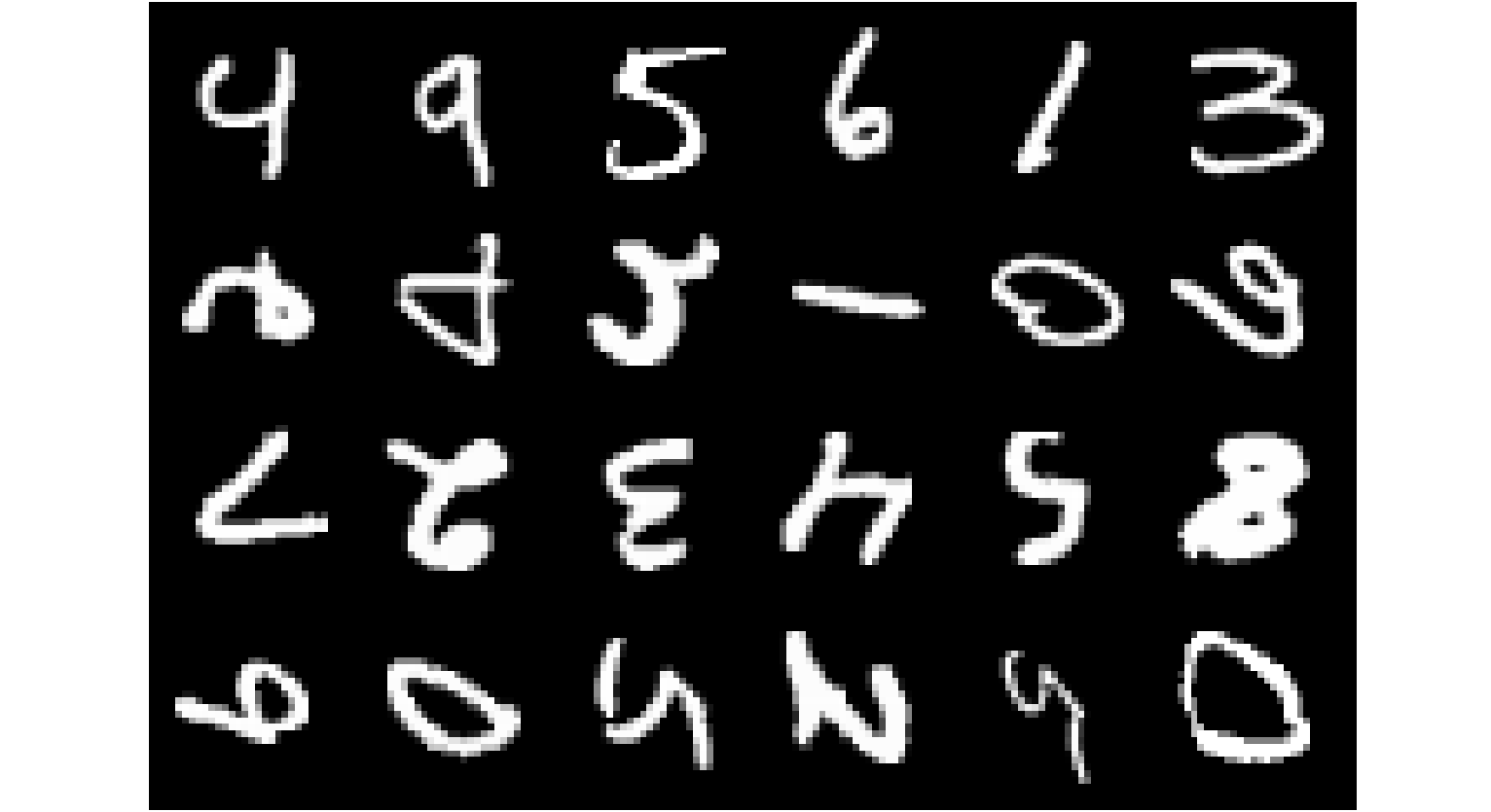
Figure 2. Examples of rotated MNIST dataset. Each row contains a collection of samples from one particular rotation.

Baselines & Implementations: We compare our FedCBO algorithm with three baseline algorithms: IFCA [15], FedAvg [28], and a local model training scheme. We use fully connected neural networks with a single hidden layer of size $200$ and ReLU activation as base model. We set the total number of agents $N=1200$ and the number of communication rounds $T=100$. In each communication round, all agents participate in the training, i.e., $|G_{n}|=N$ for all $n$. When an agent trains its own model on its local dataset (local update step in each round), we run $\tau=10$ epochs of stochastic gradient descent (SGD) with a learning rate of $\gamma=0.1$ and momentum of $0.9$. In the following, we provide some implementation details for each baseline algorithm:

• FedCBO: We set the model download budget $M=200$. We choose the hyperparameters $\lambda_{1}=10$, $\lambda_{2}=1$ and $\alpha=10$. For the $\varepsilon$-greedy sampling, we use the decay scheme $\varepsilon(n)=\max\{0.5-0.01n,0.1\}$, i.e., the initial random sample proportion $\varepsilon=0.5$. This parameter is decreased by $0.01$ at each communication round until it reaches the threshold $0.1$.

• IFCA [15]: We set the number of models initialized at the global server to equal the number of underlying clusters ($k=4$) as suggested in [15] for a fair comparison. This should provide the best result for the IFCA algorithm.

• FedAvg [28]: The algorithm tries to train a single global model that works for all the local distributions. Hence, in the model aggregation step, the local models trained by the agents are averaged to obtain the updated global model.

• Local model training: Agents train their own model using only their local data and with no communication with the global server or to any of the other agents. To ensure a fair comparison, each agent trains its model for a total of $T*\tau=1000$ epochs.

Remark 5.

Notice that in FedCBO we do not have to input the number of underlying clusters $k$, in contrast to IFCA where we need to input this value or an estimate thereof.

For FedCBO and the local model training scheme, we perform inference by testing the trained model on the test data with the same distribution as their training data (i.e., data points with the same rotation). For IFCA and FedAvg, following [15], we run inference on all learned models ($k$ models for IFCA and one model for FedAvg) on each data distribution and calculate the accuracy of the model that produces the smallest loss value. We conduct experiments with $5$ different random seeds for all the algorithms and report the average accuracy and standard deviation.

Experimental Results: The test results are summarized in Table 1. We observe that our FedCBO algorithm outperforms the three baseline methods. Although the IFCA algorithm can gradually estimate the cluster identities of users correctly and average over users’ models that are estimated to belong to the same clusters, it gives models the same weights during the model aggregation step, thus preventing the algorithm from further utilizing the relative similarities between different models. In contrast, as we run the FedCBO algorithm, we observe that during the (local) model aggregation steps, agents successfully select models from other users having the same data distribution (as discussed in Remark 6) and assign different importance (weights) to the downloaded models using (19) during the aggregation steps. In this way, each user can better utilize the most beneficial models from others. We attribute this averaging scheme (19) as one of the reasons why our FedCBO method outperforms the IFCA algorithm. As pointed out in [15], the FedAvg baseline performs worse than FedCBO and IFCA as it tries to fit heterogeneous data using one model and thus cannot provide cluster-wise predictions. Since each agent only stores a small amount of data, the local model training scheme can easily overfit to the local dataset. This explains why it produces the worst performance among all other methodologies.

Table 1. Test accuracy $\pm$ standard deviation % on rotated MNIST.

FedCBO	IFCA	FedAvg	Local
$\bm{96.51\pm 0.04}$	$94.44\pm 0.01$	$85.50\pm 0.19$	$81.27\pm 0.02$

Remark 6.

To verify the correctness of the sampling scheme in FedCBO, we define the successful selection rate (SR) for agent $j$ at iteration $n$ as follows:

(22) $$\text{SR}_{n}^{j}:=\frac{\text{Number of selected agents in the same cluster as agent $j$}}{\text{Total number of selected agents}},$$

where the total number of selected agents equals the model download budget $M$. During the FedCBO algorithm, we calculate the average successful selection rate $\text{SR}_{n}:=\frac{1}{N}\sum_{j=1}^{N}\text{SR}_{n}^{j}$ at each communication round $n$, which corresponds to the blue curve in Fig. 3. Meanwhile, when implementing the $\varepsilon$-greedy sampling, we set the random exploration proportion $\varepsilon$ to $0.5$ at $n=0$ and use a decay scheme of $\varepsilon(n)=\max\{0.5-0.01n,0.1\}$. Hence we can calculate the oracle expected successful selection rate at each round: this is shown as the orange curve in Fig. 3. We note that the empirical average successful SR (blue curve) is very close to the best expected successful SR (orange curve). This indicates that our FedCBO algorithm can successfully identify the agents with the same data distributions. We leave the task of designing better sampling strategies to close the gap between empirical successful SR and oracle successful SR to future work.

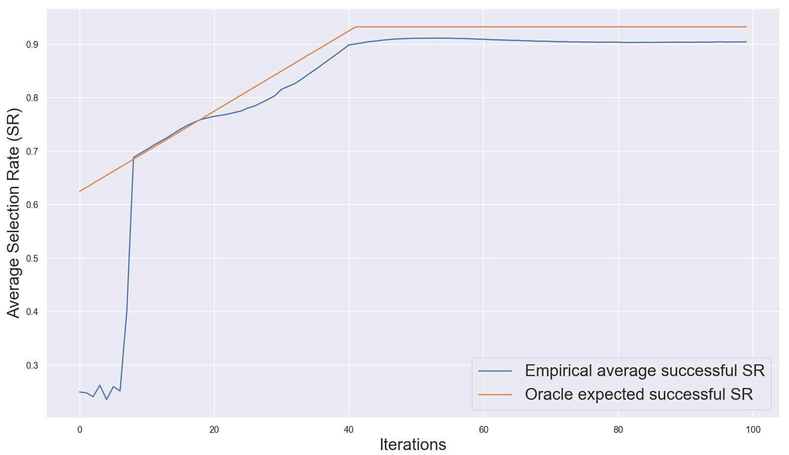
Figure 3. Average successful selection rate (SR) at each communication round.

3. Well-posedness of mean-field equations

In this section we prove Theorem 2.1. We present the details in the case in which the loss functions are assumed to be bounded. The proof for the quadratic growth case is similar, and we refer the reader to the Appendix for more details.

Lemma 3.1.

Let $L_{1},L_{2}$ satisfy Assumption 1 and let $\nu^{1},\nu^{2}\in\mathcal{C}([0,T],\mathcal{P}_{2}(\mathbb{R}^{d}))$ be such that $\sup_{t\in[0,T]}\int|\theta|^{4}d\nu_{t}^{1}\leq K$, $\sup_{t\in[0,T]}\int|\theta|^{4}d\nu_{t}^{2}\leq K$. Let us denote by $\overline{L}_{1},\overline{L}_{2}$ the supremum of each of the loss functions. Let $w_{1},w_{2}>0$ be such that $w_{1}+w_{2}=1$, and let $\nu:=w_{1}\nu^{1}+w_{2}\nu^{2}$. Then, for all $s,t\in(0,T)$, the following stability estimates hold

(23) $$|m_{L_{k}}^{\alpha}[\nu_{t}]-m_{L_{k}}^{\alpha}[\nu_{s}]|\leq C\bigg{(}w_{1}W_{2}(\nu_{t}^{1},\nu_{s}^{1})+w_{2}W_{2}(\nu_{t}^{2},\nu_{s}^{2})\bigg{)},$$

for $k=1,2$ and for a constant $C$ that depends only on $\alpha,M_{L_{1}},M_{L_{2}}$ and $K$.

Proof.

For $k=1,2$ and $s,t\in[0,T]$, one can compute the difference

$$|m_{L_{k}}^{\alpha}[\nu_{t}]-m_{L_{k}}^{\alpha}[\nu_{s}]| =|\frac{\int\theta w_{L_{k}}^{\alpha}d\nu_{t}}{\|w_{L_{k}}^{\alpha}\|_{\mathbb{L}^{1}(\nu_{t})}}-\frac{\int\theta w_{L_{k}}^{\alpha}d\nu_{s}}{\|w_{L_{k}}^{\alpha}\|_{\mathbb{L}^{1}(\nu_{s})}}|$$

$$\leq\frac{1}{\|w_{L_{k}}^{\alpha}\|_{\mathbb{L}^{1}(\nu_{t})}}|\int\theta w_{L_{k}}^{\alpha}d\nu_{t}-\int\theta w_{L_{k}}^{\alpha}d\nu_{s}|+|\int\theta w_{L_{k}}^{\alpha}d\nu_{s}||\frac{1}{\|w_{L_{k}}^{\alpha}\|_{\mathbb{L}^{1}(\nu_{t})}}-\frac{1}{\|w_{L_{k}}^{\alpha}\|_{\mathbb{L}^{1}(\nu_{s})}}|$$

$$=:A_{1}+A_{2}.$$

To estimate $A_{1}$, note that

(24) $$|\int\theta w_{L_{k}}^{\alpha}d\nu_{t}-\int\theta w_{L_{k}}^{\alpha}d\nu_{s}|\leq w_{1}|\int\theta w_{L_{k}}^{\alpha}d\nu_{t}^{1}-\int\theta w_{L_{k}}^{\alpha}d\nu_{s}^{1}|+w_{2}|\int\theta w_{L_{k}}^{\alpha}d\nu_{t}^{2}-\int\theta w_{L_{k}}^{\alpha}d\nu_{s}^{2}|.$$

Let us take a look at the first term on the right-hand side.

$$|\int\theta w_{L_{k}}^{\alpha}(\theta)d\nu_{t}^{1}(\theta)-\int\hat{\theta}w_{L_{k}}^{\alpha}(\hat{\theta})d\nu_{s}^{1}(\hat{\theta})|=|\int\int\big{[}\theta w_{L_{k}}^{\alpha}(\theta)-\hat{\theta}w_{L_{k}}^{\alpha}(\hat{\theta})\big{]}d\pi(\theta,\hat{\theta})|,$$

where $\pi$ is an arbitrary coupling between $\nu_{t}^{1}$ and $\nu_{s}^{1}$. Denote $h(\theta)-h(\hat{\theta}):=\theta w_{L_{k}}^{\alpha}(\theta)-\hat{\theta}w_{L_{k}}^{\alpha}(\hat{\theta})$, then by Assumption 1 on $L_{k}$, we have

$$|h(\theta)-h(\hat{\theta})| =|w_{L_{k}}^{\alpha}(\theta)(\theta-\hat{\theta})+\hat{\theta}\big{[}w_{L_{k}}^{\alpha}(\theta)-w_{L_{k}}^{\alpha}(\hat{\theta})\big{]}|$$

$$\leq\exp(-\alpha\underline{L_{k}})|\theta-\hat{\theta}|+\alpha\exp(-\alpha\underline{L_{k}})M_{L_{k}}|\hat{\theta}|(|\theta|+|\hat{\theta}|)|\theta-\hat{\theta}|.$$

Therefore, choosing $\pi$ to be an optimal coupling between $\nu_{t}^{1}$ and $\nu_{s}^{1}$ for the $W_{2}$-distance, we obtain

$$|\int\theta w_{L_{k}}^{\alpha}(\theta)d\nu_{t}^{1}(\theta)-\int\hat{\theta}w_{L_{k}}^{\alpha}(\hat{\theta})d\nu_{s}^{1}(\hat{\theta})| \leq\iint\exp(-\alpha\underline{L_{k}})\big{(}1+\alpha M_{L_{k}}|\hat{\theta}|(|\theta|+|\hat{\theta}|)\big{)}|\theta-\hat{\theta}|)d\pi$$

$$\leq \bigg{(}\iint\exp(-2\alpha\underline{L_{k}})\big{(}1+\alpha M_{L_{k}}|\hat{\theta}|(|\theta|+|\hat{\theta}|)\big{)}^{2}d\pi\bigg{)}^{\frac{1}{2}}\bigg{(}\iint|\theta-\hat{\theta}|^{2}d\pi\bigg{)}^{\frac{1}{2}}$$

$$\leq \exp(-\alpha\underline{L_{k}})\alpha M_{L_{k}}p_{K}\bigg{(}\iint|\theta-\hat{\theta}|^{2}d\pi\bigg{)}^{\frac{1}{2}}$$

$$= \exp(-\alpha\underline{L_{k}})\alpha M_{L_{k}}p_{K}W_{2}(\nu_{t}^{1},\nu_{s}^{1})\,.$$

Here $p_{K}$ is a polynomial in $K$. Similarly, we deduce

$$|\int\theta w_{L_{k}}^{\alpha}d\nu_{t}^{2}-\int\theta w_{L_{k}}^{\alpha}d\nu_{s}^{2}|\leq\exp(-\alpha\underline{L_{k}})\alpha M_{L_{k}}p_{K}W_{2}(\nu_{t}^{2},\nu_{s}^{2})\,.$$

Therefore, we conclude

$$|\int\theta w_{L_{k}}^{\alpha}d\nu_{t}-\int\theta w_{L_{k}}^{\alpha}d\nu_{s}| \leq w_{1}|\int\theta w_{L_{k}}^{\alpha}d\nu_{t}^{1}-\int\theta w_{L_{k}}^{\alpha}d\nu_{s}^{1}|+w_{2}|\int\theta w_{L_{k}}^{\alpha}d\nu_{t}^{2}-\int\theta w_{L_{k}}^{\alpha}d\nu_{s}^{2}|$$

$$\leq\exp(-\alpha\underline{L_{k}})\alpha M_{L_{k}}p_{K}\big{(}w_{1}W_{2}(\nu_{t}^{1},\nu_{s}^{1})+w_{2}W_{2}(\nu_{t}^{2},\nu_{s}^{2})\big{)}\,,$$

and

$$A_{1}:=\frac{1}{\|w_{L_{k}}^{\alpha}\|_{\mathbb{L}^{1}(\nu_{t})}}|\int\theta w_{L_{k}}^{\alpha}d\nu_{t}-\int\theta w_{L_{k}}^{\alpha}d\nu_{s}|\leq\exp(\alpha(\overline{L_{k}}-\underline{L_{k}}))\alpha M_{L_{k}}p_{K}\big{(}w_{1}W_{2}(\nu_{t}^{1},\nu_{s}^{1})+w_{2}W_{2}(\nu_{t}^{2},\nu_{s}^{2})\big{)}\,.$$

For the second term $A_{2}$, we have

$$A_{2}:=|\int\theta w_{L_{k}}^{\alpha}d\nu_{s}||\frac{1}{\|w_{L_{k}}^{\alpha}\|_{\mathbb{L}^{1}(\nu_{t})}}-\frac{1}{\|w_{L_{k}}^{\alpha}\|_{\mathbb{L}^{1}(\nu_{s})}}|=\frac{\int\theta w_{L_{k}}^{\alpha}d\nu_{s}}{\|w_{L_{k}}^{\alpha}\|_{\mathbb{L}^{1}(\nu_{t})}\|w_{L_{k}}^{\alpha}\|_{\mathbb{L}^{1}(\nu_{s})}}|\int w_{L_{k}}^{\alpha}d\nu_{t}-\int w_{L_{k}}^{\alpha}d\nu_{s}|.$$

Similar to the estimation in (24), we have

$$|\int w_{L_{k}}^{\alpha}d\nu_{t}-\int w_{L_{k}}^{\alpha}d\nu_{s}|\leq\exp(-\alpha\underline{L_{k}})\alpha M_{L_{k}}q_{K}\bigg{(}w_{1}W_{2}(\nu_{t}^{1},\nu_{s}^{1})+w_{2}W_{2}(\nu_{t}^{2},\nu_{s}^{2})\bigg{)},$$

where $q_{K}$ is a polynomial on $K$. Then,

$$A_{2} =\frac{\int\theta w_{L_{k}}^{\alpha}d\nu_{s}}{\|w_{L_{k}}^{\alpha}\|_{\mathbb{L}^{1}(\nu_{t})}\|w_{L_{k}}^{\alpha}\|_{\mathbb{L}^{1}(\nu_{s})}}|\int w_{L_{k}}^{\alpha}d\nu_{t}-\int w_{L_{k}}^{\alpha}d\nu_{s}|$$

$$\leq C_{K_{k}}\exp(\alpha\overline{L_{k}})\exp(-\alpha\underline{L_{k}})\alpha M_{L_{k}}q_{K}\bigg{(}w_{1}W_{2}(\nu_{t}^{1},\nu_{s}^{1})+w_{2}W_{2}(\nu_{t}^{2},\nu_{s}^{2})\bigg{)}$$

$$=C_{K_{k}}\exp(\alpha(\overline{L_{k}}-\underline{L_{k}}))\alpha M_{L_{k}}q_{K}\bigg{(}w_{1}W_{2}(\nu_{t}^{1},\nu_{s}^{1})+w_{2}W_{2}(\nu_{t}^{2},\nu_{s}^{2})\bigg{)}.$$

Combining the estimates for $A_{1}$ and $A_{2}$, we obtain

$$|m_{L_{k}}^{\alpha}[\nu_{t}]-m_{L_{k}}^{\alpha}[\nu_{s}]|\leq C\bigg{(}w_{1}W_{2}(\nu_{t}^{1},\nu_{s}^{1})+w_{2}W_{2}(\nu_{t}^{2},\nu_{s}^{2})\bigg{)},$$

where $C:=\max\bigg{\{}\exp(\alpha(\overline{L_{1}}-\underline{L_{1}}))\alpha M_{L_{1}}(p_{K}+C_{K_{1}}q_{K}),\exp(\alpha(\overline{L_{2}}-\underline{L_{2}}))\alpha M_{L_{2}}(p_{K}+C_{K_{2}}q_{K})\bigg{\}}$. ∎

Proof of Theorem 2.1.

The proof is split into several steps.

Step 1: For a given pair $u^{1},u^{2}\in\mathcal{C}([0,T],\mathbb{R}^{d})$, we may apply standard theory of SDEs to conclude that there exists a unique strong solution to the SDE

(25a) $$dY_{t}^{1}=-\lambda_{1}(Y_{t}^{1}-u_{t}^{1})dt-\lambda_{2}\nabla L_{1}(Y_{t}^{1})dt+\sigma_{1}|Y_{t}^{1}-u_{t}^{1}|dB_{t}^{1}+\sigma_{2}|\nabla L_{1}(Y_{t}^{1})|d\widetilde{B}_{t}^{1}$$

(25b) $$dY_{t}^{2}=-\lambda_{1}(Y_{t}^{2}-u_{t}^{2})dt-\lambda_{2}\nabla L_{2}(Y_{t}^{2})dt+\sigma_{1}|Y_{t}^{2}-u_{t}^{2}|dB_{t}^{2}+\sigma_{2}|\nabla L_{2}(Y_{t}^{2})|d\widetilde{B}_{t}^{2},$$

for initial conditions $Y^{1}_{0}\sim\rho_{0}^{1}$ and $Y_{0}^{2}\sim\rho_{2}$ (independent of each other), where $\rho_{0}^{1},\rho_{0}^{2}\in\mathcal{P}_{4}(\mathbb{R}^{d})$. Let $\nu_{t}^{1}=\text{Law}(Y_{t}^{1})$ and $\nu_{t}^{2}=\text{Law}(Y_{t}^{2})$ be the laws of $Y_{t}^{1}$ and $Y_{t}^{2}$, respectively. Since the variables $Y^{1},Y^{2}$ take values in $\mathcal{C}([0,T],\mathbb{R}^{d})$, it follows that $\nu^{1},\nu^{2}\in\mathcal{C}([0,T],\mathcal{P}(\mathbb{R}^{d}))$. Moreover, $\nu^{1}_{t},\nu^{2}_{t}$ satisfy the following system of Fokker-Planck equations (in weak form):

(26a) $$\frac{d}{dt}\int\varphi d\nu_{t}^{1}=\int\bigg{[}\big{(}-\lambda_{1}(\theta-u_{t}^{1})-\lambda_{2}\nabla L_{1}(\theta)\big{)}\cdot\nabla\varphi+\big{(}\frac{\sigma_{1}^{2}}{2}|\theta-u_{t}^{1}|^{2}+\frac{\sigma_{2}^{2}}{2}|\nabla L_{1}(\theta)|^{2}\big{)}\Delta\varphi\bigg{]}d\nu_{t}^{1},$$

(26b) $$\frac{d}{dt}\int\varphi d\nu_{t}^{2}=\int\bigg{[}\big{(}-\lambda_{1}(\theta-u_{t}^{2})-\lambda_{2}\nabla L_{2}(\theta)\big{)}\cdot\nabla\varphi+\big{(}\frac{\sigma_{1}^{2}}{2}|\theta-u_{t}^{2}|^{2}+\frac{\sigma_{2}^{2}}{2}|\nabla L_{2}(\theta)|^{2}\big{)}\Delta\varphi\bigg{]}d\nu_{t}^{2},$$

for all $\varphi\in\mathcal{C}_{c}^{2}(\mathbb{R}^{d})$. Let us consider the product space $\mathcal{C}([0,T],\mathbb{R}^{d})\times\mathcal{C}([0,T],\mathbb{R}^{d})$ endowed with the norm $\|\cdot\|$ defined as

$$\|(f,g)\|:=\|f\|_{\infty}+\|g\|_{\infty},$$

where $f,g\in\mathcal{C}([0,T],\mathbb{R}^{d})$ and $\|f\|_{\infty}:=\sup_{t\in[0,T]}|f_{t}|$. Let $P_{k}:\mathcal{C}([0,T],\mathbb{R}^{d})\times\mathcal{C}([0,T],\mathbb{R}^{d})\rightarrow\mathcal{C}([0,T],\mathbb{R}^{d})$ be the projection onto the $k$-th coordinate for $k=1,2$. That is, for any $(f,g)\in\mathcal{C}([0,T],\mathbb{R}^{d})\times\mathcal{C}([0,T],\mathbb{R}^{d})$, $P_{1}(f,g)=f$ and $P_{2}(f,g)=g$. Notice that $m_{L_{k}}[\nu]\in\mathcal{C}([0,T],\mathbb{R}^{d})$ for $k=1,2$ and thus we can define the map

$$\mathcal{T}:\mathcal{C}([0,T],\mathbb{R}^{d})\times\mathcal{C}([0,T],\mathbb{R}^{d}) \longrightarrow\mathcal{C}([0,T],\mathbb{R}^{d})\times\mathcal{C}([0,T],\mathbb{R}^{d}),$$

$$(u^{1},u^{2}) \longrightarrow\mathcal{T}(u^{1},u^{2})=(m_{L_{1}}^{\alpha}[\nu],m_{L_{2}}^{\alpha}[\nu]),$$

where $\nu=w_{1}\nu^{1}+w_{2}\nu^{2}$.

Next, we show that $\mathcal{T}$ has a unique fixed point.

Step 2: First, we show that $\mathcal{T}$ is compact, i.e., any bounded sequence $\{(f_{n},g_{n})\}_{n\in\mathbb{N}}$ in $\mathcal{C}([0,T],\mathbb{R}^{d})\times\mathcal{C}([0,T],\mathbb{R}^{d})$ is precompact. Let $(\varphi_{n},\psi_{n}):=\mathcal{T}(f_{n},g_{n})$. It is sufficient to show that each of the sequences $\{\varphi_{n}\}_{n\in\mathbb{N}}$ and $\{\psi_{n}\}_{n\in\mathbb{N}}$ is precompact. We show the details for the sequence $\{\varphi_{n}\}_{n\in\mathbb{N}}$. Since $\rho_{0}^{1},\rho_{0}^{2}\in\mathcal{P}_{4}(\mathbb{R}^{d})$, standard theory of SDEs (see, e.g., Chapter $7$ of [1]) provides a fourth-order moment estimate for solutions to (25a) and (25b) of the form

$$\mathbb{E}|Y_{t}^{1}|^{\color[rgb]{1,0,0}4\normalcolor}\leq(1+\mathbb{E}|Y_{0}^{1}|^{4})\exp(ct)\qquad\text{and}\qquad\mathbb{E}|Y_{t}^{2}|^{\color[rgb]{1,0,0}4}\leq(1+\mathbb{E}|Y_{0}^{2}|^{4})\exp(ct),$$

for some constant $c>0$ only depending on $\|u^{1}\|_{\infty}$ and $\|u^{2}\|_{\infty}$. In particular,

$$\sup_{t\in[0,T]}\int|x|^{4}d\nu^{1}_{t},\sup_{t\in[0,T]}\int|x|^{4}d\nu^{2}_{t}\leq K$$

for some $K<\infty$. On the other hand, for any $t>s,t,s\in(0,T)$, the Itô isometry and Cauchy-Schwarz inequality yield

$$\mathbb{E}|Y_{t}^{1}-Y_{s}^{1}|^{2} =\mathbb{E}\bigg{[}\int_{s}^{t}\big{(}-\lambda_{1}(Y_{\tau}^{1}-u_{\tau}^{1})-\lambda_{2}\nabla L_{1}(Y_{\tau}^{1})\big{)}d\tau+\int_{s}^{t}\sigma_{1}|Y_{\tau}^{1}-u_{\tau}^{1}|dB_{\tau}^{1}+\int_{s}^{t}\sigma_{2}|\nabla L_{1}(Y_{\tau}^{1})|d\widetilde{B}_{\tau}^{1}\bigg{]}^{2}$$

$$\leq 2\mathbb{E}\bigg{[}\int_{s}^{t}\big{(}-\lambda_{1}(Y_{\tau}^{1}-u_{\tau}^{1})-\lambda_{2}\nabla L_{1}(Y_{\tau}^{1})\big{)}d\tau\bigg{]}^{2}+2\mathbb{E}\bigg{[}\int_{s}^{t}\big{(}\sigma^{2}|Y_{\tau}^{1}-u_{\tau}^{1}|^{2}+\sigma_{2}^{2}|\nabla L_{1}(Y_{\tau}^{1})|^{2}\big{)}d\tau\bigg{]}$$

$$\leq 2\lambda_{1}^{2}|t-s|\mathbb{E}\big{[}\int_{s}^{t}|Y_{\tau}^{1}-u_{\tau}^{1}|^{2}d\tau\big{]}+2\lambda_{2}^{2}|t-s|\mathbb{E}\big{[}\int_{s}^{t}|\nabla L_{1}(Y_{\tau}^{1})|^{2}d\tau\big{]}$$

$$\quad+\mathbb{E}\bigg{[}\int_{s}^{t}\big{(}\sigma^{2}|Y_{\tau}^{1}-u_{\tau}^{1}|^{2}+\sigma_{2}^{2}|\nabla L_{1}(Y_{\tau}^{1})|^{2}\big{)}d\tau\bigg{]}$$

$$\leq 4\lambda_{1}^{2}(K+\|u^{1}\|_{\infty}^{2})T|t-s|+2\lambda_{2}^{2}C_{\nabla L_{1}}^{2}T|t-s|+2\sigma_{1}^{2}(K+\|u^{1}\|_{\infty}^{2})|t-s|+\sigma_{2}^{2}C_{\nabla L_{1}}^{2}|t-s|$$

$$=:C_{1}|t-s|.$$

Similarly, $\mathbb{E}|Y_{t}^{2}-Y_{s}^{2}|^{2}\leq C_{2}|t-s|$ for a constant $C_{2}>0$. Therefore, $W_{2}(\nu_{t}^{1},\nu_{s}^{1})\leq c_{1}|t-s|^{\frac{1}{2}}$ and $W_{2}(\nu_{t}^{2},\nu_{s}^{2})\leq c_{2}|t-s|^{\frac{1}{2}}$, for some constants $c_{1},c_{2}>0$ only depending on $\|u^{1}\|_{\infty}$ and $\|u^{2}\|_{\infty}$. Applying Lemma 3.1, we obtain

$$|m_{L_{1}}^{\alpha}[\nu_{t}]-m_{L_{1}}^{\alpha}[\nu_{s}]|\leq C(w_{1}c_{1}+w_{2}c_{2})|t-s|^{\frac{1}{2}},$$

which proves that $t\rightarrow m_{L_{1}}^{\alpha}[\nu_{t}]$ is Hölder continuous with exponent $\frac{1}{2}$. From this we can conclude that $\{\varphi_{n}\}_{n\in\mathbb{N}}$ is precompact due to the compact embedding $\mathcal{C}^{0,1/2}([0,T],\mathbb{R}^{d})\hookrightarrow\mathcal{C}([0,T],\mathbb{R}^{d})$, where $\mathcal{C}^{0,1/2}([0,T],\mathbb{R}^{d})$ is the space of $\frac{1}{2}$-Hölder continuous functions from $[0,T]$ into $\mathbb{R}^{d}$.

Step 3: Next, we verify the conditions in the Leray-Schauder fixed point theorem. For that purpose, suppose the pair $(u^{1},u^{2})\in\mathcal{C}([0,T],\mathbb{R}^{d})\times\mathcal{C}([0,T],\mathbb{R}^{d})$ satisfies $(u^{1},u^{2})=\tau\mathcal{T}(u^{1},u^{2})$ for some $\tau\in[0,1]$. In particular, there exist $\nu_{1},\nu_{2}\in\mathcal{C}([0,T],\mathcal{P}_{2}(\mathbb{R}^{d}))$ satisfying (26a) and (26b), respectively, such that $(u^{1},u^{2})=\tau(m_{L_{1}}^{\alpha}[\nu],m_{L_{2}}^{\alpha}[\nu])$, where $\nu=w_{1}\nu_{1}+w_{2}\nu_{2}$. Due to the boundedness assumption on $L_{1}$, we have for all $t\in(0,T)$

(27) $$|u_{t}^{1}|^{2}=\tau^{2}|m_{L_{1}}[\nu]|^{2}\leq\tau^{2}\exp(\alpha(\overline{L_{1}}-\underline{L_{1}}))\int|x|^{2}d\nu_{t}=\tau^{2}\exp(\alpha(\overline{L_{1}}-\underline{L_{1}}))\bigg{(}w_{1}\int|x|^{2}d\nu_{t}^{1}+w_{2}\int|x|^{2}d\nu_{t}^{2}\bigg{)}.$$

A computation of the second moment of $\nu_{t}^{1}$ gives

$$\frac{d}{dt}\int|\theta|^{2}d\nu_{t}^{1} =\int\bigg{[}\big{(}-\lambda_{1}(\theta-u_{t}^{1})-\lambda_{2}\nabla L_{1}(\theta)\big{)}\cdot 2\theta+2d\big{(}\frac{\sigma_{1}^{2}}{2}|\theta-u_{t}^{1}|^{2}+\frac{\sigma_{2}^{2}}{2}|\nabla L_{1}(\theta)|^{2}\big{)}\bigg{]}d\nu_{t}^{1}$$

$$=\int\bigg{[}-2\lambda_{1}|\theta|^{2}+2\lambda_{1}\theta\cdot u_{t}^{1}-2\lambda_{2}\theta\cdot\nabla L_{1}(\theta)+d\sigma_{1}^{2}(|\theta|^{2}-2\theta\cdot u_{t}^{1}+|u_{t}^{1}|^{2})+d\sigma_{2}^{2}|\nabla L_{1}(\theta)|^{2}\bigg{]}d\nu_{t}^{1}$$

$$\leq\int\bigg{[}(d\sigma_{1}^{2}-2\lambda_{1}+|\gamma|+\lambda_{2})|\theta|^{2}+(d\sigma_{1}^{2}+|\gamma|)|u_{t}^{1}|^{2}+(\lambda_{2}+d\sigma_{2}^{2})|\nabla L_{1}(\theta)|^{2}\bigg{]}d\nu_{t}^{1}$$

$$\leq(d\sigma_{1}^{2}-2\lambda_{1}+|\gamma|+\lambda_{2})\int|\theta|^{2}d\nu_{t}^{1}+(d\sigma_{1}^{2}+|\gamma|)|u_{t}^{1}|^{2}+(\lambda_{2}+d\sigma_{2}^{2})C_{\nabla L_{1}}^{2}$$

$$\leq(d\sigma_{1}^{2}+|\gamma|+\lambda_{2})\big{(}1+\exp(\alpha(\overline{L_{1}}-\underline{L_{1}}))\big{)}\bigg{(}\int|\theta|^{2}d\nu_{t}^{1}+\int|\theta|^{2}d\nu_{t}^{2}\bigg{)}+(\lambda_{2}+d\sigma_{2}^{2})C_{\nabla L_{1}}^{2},$$

where $\gamma:=\lambda_{1}-d\sigma_{1}^{2}$. Similarly,

$$\frac{d}{dt}\int|\theta|^{2}d\nu_{t}^{2}\leq(d\sigma_{1}^{2}+|\gamma|+\lambda_{2})\big{(}1+\exp(\alpha(\overline{L_{2}}-\underline{L_{2}}))\big{)}\bigg{(}\int|\theta|^{2}d\nu_{t}^{1}+\int|\theta|^{2}d\nu_{t}^{2}\bigg{)}+(\lambda_{2}+d\sigma_{2}^{2})C_{\nabla L_{2}}^{2}.$$

Adding the above two inequalities we conclude that

$$\frac{d}{dt}\bigg{(}\int|\theta|^{2}d\nu_{t}^{1}+\int|\theta|^{2}d\nu_{t}^{2}\bigg{)}\leq C_{1}\bigg{(}\int|\theta|^{2}d\nu_{t}^{1}+\int|\theta|^{2}d\nu_{t}^{2}\bigg{)}+C_{2},$$

for some constants $C_{1},C_{2}>0$. Using Grönwall’s inequality we obtain

$$\int|\theta|^{2}d\nu_{t}^{1}+\int|\theta|^{2}d\nu_{t}^{2}\leq\bigg{(}\int|\theta|^{2}d\nu_{0}^{1}+\int|\theta|^{2}d\nu_{0}^{2}\bigg{)}\exp(C_{1}t)+\frac{C_{2}}{C_{1}}\big{(}\exp(C_{1}t)-1\big{)}.$$

Then, from (27), we conclude that there is a constant $q_{1}>0$ such that $\|u^{1}\|_{\infty}<q_{1}$. A similar bound holds for $\|u^{2}\|_{\infty}$, i.e., there is a constant $q_{2}>0$ such that $\|u^{2}\|_{\infty}<q_{2}$. Hence, $\|(u^{1},u^{2})\|=\|u^{1}\|_{\infty}+\|u^{2}\|_{\infty}<q_{1}+q_{2}$. We may now invoke the Leray-Schauder fixed point theorem (Section 9.2 in [11]) to conclude that there exists a fixed point $(u^{1},u^{2})$ for the mapping $\mathcal{T}$ and thereby a solution of (25a) and (25b).

Step 4: As for uniqueness, we first note that a fixed point $(u^{1},u^{2})$ of $\mathcal{T}$ must satisfy $\|(u^{1},u^{2})\|<q$. Hence, the fourth-order moment estimates provided in Step 2 hold and $\sup_{t\in[0,T]}\int|x|^{4}d\nu_{t}^{k}\leq K<\infty$ for $k=1,2$. Now suppose we have two fixed points $(u^{1},u^{2})$ and $(\hat{u}^{1},\hat{u}^{2})$ with

$$\|(u^{1},u^{2})\|,\|(\hat{u}^{1},\hat{u}^{2})\|<q,\qquad\sup_{t\in[0,T]}\int|x|^{4}d\nu_{t}^{k},\sup_{t\in[0,T]}\int|x|^{4}d\hat{\nu}_{t}^{k}\leq K\quad\text{for $k=1,2$,}$$

and consider their corresponding processes $(Y_{t}^{1},Y_{t}^{2}),(\hat{Y}_{t}^{1},\hat{Y}_{t}^{2})$, which satisfy (25a) and (25b) with the same Brownian motions for both $k=1,2$. Taking the differences $z_{t}^{k}:=Y_{t}^{k}-\hat{Y}_{t}^{k}$ for $k=1,2$, we obtain

$$z_{t}^{k} =z_{0}^{k}+\int_{0}^{t}\big{(}-\lambda_{1}z_{s}^{k}+\lambda_{1}(u_{s}^{k}-\hat{u}_{s}^{k})-\lambda_{2}(\nabla L_{k}(Y_{s}^{k})-\nabla L_{k}(\hat{Y}_{s}^{k}))\big{)}ds$$

$$\quad+\sigma_{1}\int_{0}^{t}\big{(}|Y_{s}^{k}-u_{s}^{k}|-|\hat{Y}_{s}^{k}-\hat{u}_{s}^{k}|\big{)}dB_{s}^{k}+\sigma_{2}\int_{0}^{t}\big{(}|\nabla L_{k}(Y_{s}^{k})|-|\nabla L_{k}(\hat{Y}_{s}^{k})|\big{)}d\widetilde{B}_{s}^{k}.$$

Squaring both sides, taking expectations, and using Itô isometry we obtain

$$\mathbb{E}|z_{t}^{k}|^{2} =\mathbb{E}\bigg{[}z_{0}^{k}+\int_{0}^{t}\big{(}-\lambda_{1}z_{s}^{k}+\lambda_{1}(u_{s}^{k}-\hat{u}_{s}^{k})-\lambda_{2}(\nabla L_{k}(Y_{s}^{k})-\nabla L_{k}(\hat{Y}_{s}^{k}))\big{)}ds$$

$$\qquad+\sigma_{1}\int_{0}^{t}\big{(}|Y_{s}^{k}-u_{s}^{k}|-|\hat{Y}_{s}^{k}-\hat{u}_{s}^{k}|\big{)}dB_{s}^{k}+\sigma_{2}\int_{0}^{t}\big{(}|\nabla L_{k}(Y_{s}^{k})|-|\nabla L_{k}(\hat{Y}_{s}^{k})|\big{)}d\widetilde{B}_{s}^{k}\bigg{]}^{2}$$

$$\leq 2\mathbb{E}|z_{0}^{k}|^{2}+2t\mathbb{E}\bigg{[}\int_{0}^{t}\big{(}-\lambda_{1}z_{s}^{k}+\lambda_{1}(u_{s}^{k}-\hat{u}_{s}^{k})-\lambda_{2}(\nabla L_{k}(Y_{s}^{k})-\nabla L_{k}(\hat{Y}_{s}^{k}))\big{)}^{2}ds\bigg{]}$$

$$\quad+2\sigma_{1}^{2}\mathbb{E}\bigg{[}\int_{0}^{t}\big{(}|Y_{s}^{k}-u_{s}^{k}|-|\hat{Y}_{s}^{k}-\hat{u}_{s}^{k}|\big{)}^{2}ds\bigg{]}+2\sigma_{2}^{2}\mathbb{E}\bigg{[}\int_{0}^{t}\big{(}|\nabla L_{k}(Y_{s}^{k})|-|\nabla L_{k}(\hat{Y}_{s}^{k})|\big{)}^{2}ds\bigg{]}$$

$$\leq 2\mathbb{E}|z_{0}^{k}|^{2}+6t\lambda_{1}^{2}\int_{0}^{t}\mathbb{E}|z_{s}^{k}|^{2}ds+6t\lambda_{1}^{2}\int_{0}^{t}|u_{s}^{k}-\hat{u}_{s}^{k}|^{2}ds+6t\lambda_{2}^{2}\int_{0}^{t}\mathbb{E}\big{[}\nabla L_{k}(Y_{s}^{k})-\nabla L_{k}(\hat{Y}_{s}^{k})\big{]}^{2}ds$$

$$\quad+2\sigma_{1}^{2}\mathbb{E}\bigg{[}\int_{0}^{t}|(Y_{s}^{k}-\hat{Y}_{s}^{k})-(u_{s}^{k}-\hat{u}_{s}^{k})|^{2}ds\bigg{]}+2\sigma_{2}^{2}\mathbb{E}\bigg{[}\int_{0}^{t}|\nabla L_{k}(Y_{s}^{k})-\nabla L_{k}(\hat{Y}_{s}^{k})|^{2}ds\bigg{]}$$

$$\leq 2\mathbb{E}|z_{0}^{k}|^{2}+(6\lambda_{1}^{2}t+4\sigma_{1}^{2})\int_{0}^{t}\mathbb{E}|z_{s}^{k}|^{2}ds+(6\lambda_{1}^{2}t+4\sigma_{1}^{2})\int_{0}^{t}|u_{s}^{k}-\hat{u}_{s}^{k}|^{2}ds$$

$$\quad+6\lambda_{2}^{2}M_{\nabla L_{1}}^{2}\int_{0}^{t}\mathbb{E}|z_{s}^{k}|^{2}ds+2\sigma_{2}^{2}M_{\nabla L_{1}}^{2}\int_{0}^{t}\mathbb{E}|z_{s}^{k}|^{2}ds$$

$$=2\mathbb{E}|z_{0}^{k}|^{2}+\big{[}6\lambda_{1}^{2}t+4\sigma_{1}^{2}+M_{\nabla L_{1}}^{2}(6\lambda_{2}^{2}+2\sigma_{2}^{2})\big{]}\int_{0}^{t}\mathbb{E}|z_{s}^{k}|^{2}ds+(6\lambda_{1}^{2}t+4\sigma_{1}^{2})\int_{0}^{t}|u_{s}^{k}-\hat{u}_{s}^{k}|^{2}ds.$$

By Lemma 3.1, for $k=1,2$, we get

(28) $$|u_{s}^{k}-\hat{u}_{s}^{k}|^{2}=|m_{L_{k}}[\nu_{s}]-m_{L_{k}}[\hat{\nu}_{s}]|^{2} \leq C^{2}\big{(}w_{1}W_{2}(\nu_{s}^{1},\hat{\nu}_{s}^{1})+w_{2}W_{2}(\nu_{s}^{2},\hat{\nu}_{s}^{2})\big{)}^{2}$$

$$\leq C^{2}\big{(}w_{1}\sqrt{\mathbb{E}|z_{s}^{1}|^{2}}+w_{2}\sqrt{\mathbb{E}|z_{s}^{2}|^{2}}\big{)}^{2}$$

$$\leq 2C^{2}\big{(}\mathbb{E}|z_{s}^{1}|^{2}+\mathbb{E}|z_{s}^{2}|^{2}\big{)}.$$

We further obtain

$$\mathbb{E}|z_{t}^{1}|^{2} \leq 2\mathbb{E}|z_{0}^{1}|^{2}+\widetilde{C}_{1}\int_{0}^{t}\mathbb{E}|z_{s}^{1}|^{2}ds+\widetilde{C}_{2}\int\mathbb{E}|z_{s}^{2}|^{2}ds$$

$$\mathbb{E}|z_{t}^{2}|^{2} \leq 2\mathbb{E}|z_{0}^{2}|^{2}+\widetilde{C}_{1}\int_{0}^{t}\mathbb{E}|z_{s}^{2}|^{2}ds+\widetilde{C}_{2}\int\mathbb{E}|z_{s}^{1}|^{2}ds,$$

where $\widetilde{C}_{1}=(1+2C^{2})(6\lambda_{1}^{2}t+4\sigma_{1}^{2})+(6\lambda_{2}^{2}+2\sigma_{2}^{2})\max\{M_{\nabla L_{1}}^{2},M_{\nabla L_{2}}^{2}\}$ and $\widetilde{C}_{2}=2C^{2}(6\lambda_{1}^{2}t+4\sigma_{1}^{2})$. Combining the above two inequalities we deduce

$$\mathbb{E}|z_{t}^{1}|^{2}+\mathbb{E}|z_{t}^{2}|^{2}\leq 2\big{(}\mathbb{E}|z_{0}^{1}|^{2}+\mathbb{E}|z_{0}^{2}|^{2}\big{)}+(\widetilde{C}_{1}+\widetilde{C}_{2})\int_{0}^{t}\big{(}\mathbb{E}|z_{s}^{1}|^{2}+\mathbb{E}|z_{s}^{2}|^{2}\big{)}ds.$$

Then, by Grönwall’s inequality and the fact that $\mathbb{E}|z_{0}^{1}|^{2}=\mathbb{E}|z_{0}^{2}|^{2}=0$, we infer that $\mathbb{E}|z_{t}^{1}|^{2}+\mathbb{E}|z_{t}^{2}|^{2}=0$ for all $t\in[0,T]$. From inequality (28), we obtain $\|u^{1}-\hat{u}^{1}\|_{\infty}=\|u^{2}-\hat{u}^{2}\|_{\infty}=0$, i.e., $(u^{1},u^{2})\equiv(\hat{u}^{1},\hat{u}^{2})$, proving in this way the uniqueness. ∎

Remark 7.

Notice that the stochastic processes $Y^{1}$ and $Y^{2}$ in (25a) and (25b) are independent from each other for any input functions $(u^{1},u^{2})$. In turn, since (7a) and (7b) are realized as $(Y^{1},Y^{2})$ for a specific choice of $(u^{1},u^{2})$ (i.e., for a fixed point of $\mathcal{T}$), we conclude that the processes $\overline{\theta}^{1},\overline{\theta}^{2}$ from (7a) and (7b) are independent as stochastic processes. Notice, however, that both SDEs share parameters, e.g., the distribution $\rho$ appearing in both the drift and diffusion terms of the equations.

4. Large time behavior of mean-field equation and consensus formation

Proof of Theorem 2.3.

Let $M:=\max\{M_{\nabla L_{1}},M_{\nabla L_{2}}\}$. Using Lemma C.1 we get

(29) $$\frac{d}{dt}\big{(}\mathcal{V}(\rho_{t}^{1})+\mathcal{V}(\rho_{t}^{2})\big{)} \leq-(2\lambda_{1}-2\lambda_{2}M-d\sigma_{1}^{2}-d\sigma_{2}^{2}M^{2})\big{(}\mathcal{V}(\rho_{t}^{1})+\mathcal{V}(\rho_{t}^{2})\big{)}$$

$$\quad+\sqrt{2}(\lambda_{1}+d\sigma_{1}^{2})\bigg{(}\sqrt{\mathcal{V}(\rho_{t}^{1})}|m_{L_{1}}^{\alpha}[\rho_{t}]-\theta_{1}^{*}|+\sqrt{\mathcal{V}(\rho_{t}^{2})}|m_{L_{2}}^{\alpha}[\rho_{t}]-\theta_{2}^{*}|\bigg{)}$$

$$\quad+\frac{d\sigma_{1}^{2}}{2}\big{(}|m_{L_{1}}^{\alpha}[\rho_{t}]-\theta_{1}^{*}|^{2}+|m_{L_{2}}^{\alpha}[\rho_{t}]-\theta_{2}^{*}|^{2}\big{)}$$

$$\leq-(2\lambda_{1}-2\lambda_{2}M-d\sigma_{1}^{2}-d\sigma_{2}^{2}M^{2})\big{(}\mathcal{V}(\rho_{t}^{1})+\mathcal{V}(\rho_{t}^{2})\big{)}$$

$$\quad+\sqrt{2}(\lambda_{1}+d\sigma_{1}^{2})\big{(}|m_{L_{1}}^{\alpha}[\rho_{t}]-\theta_{1}^{*}|+|m_{L_{2}}^{\alpha}[\rho_{t}]-\theta_{2}^{*}|\big{)}\sqrt{\mathcal{V}(\rho_{t}^{1})+\mathcal{V}(\rho_{t}^{2})}$$

$$\quad+\frac{d\sigma_{1}^{2}}{2}\big{(}|m_{L_{1}}^{\alpha}[\rho_{t}]-\theta_{1}^{*}|^{2}+|m_{L_{2}}^{\alpha}[\rho_{t}]-\theta_{2}^{*}|^{2}\big{)}.$$

Let $T_{\alpha}\geq 0$ be given by

(30) $$T_{\alpha}:=\sup\big{\{}t\geq 0:\mathcal{V}(\rho_{t^{\prime}}^{1})+\mathcal{V}(\rho_{t^{\prime}}^{2})>\varepsilon,|m_{L_{1}}^{\alpha}[\rho_{t^{\prime}}]-\theta_{1}^{*}|+|m_{L_{2}}^{\alpha}[\rho_{t^{\prime}}]-\theta_{2}^{*}|<C(t^{\prime})\;\,\forall t^{\prime}\in[0,t]\big{\}},$$

where

(31) $$C(t):=C\sqrt{\mathcal{V}(\rho_{t}^{1})+\mathcal{V}(\rho_{t}^{2})}$$

with

(32) $$C:=\min\bigg{\{}\frac{\tau}{2}\frac{(2\lambda_{1}-2\lambda_{2}M-d\sigma_{1}^{2}-d\sigma_{2}^{2}M^{2})}{\sqrt{2}(\lambda_{1}+d\sigma_{1}^{2})},\sqrt{\tau\frac{(2\lambda_{1}-2\lambda_{2}M-d\sigma_{1}^{2}-d\sigma_{2}^{2}M^{2})}{d\sigma_{1}^{2}}}\bigg{\}}.$$

Then, combining (29) with (30), for all $t\in[0,T_{\alpha}]$ we have

(33) $$\frac{d}{dt}\big{(}\mathcal{V}(\rho_{t}^{1})+\mathcal{V}(\rho_{t}^{2})\big{)}\leq-(1-\tau)(2\lambda_{1}-2\lambda_{2}M-d\sigma_{1}^{2}-d\sigma_{2}^{2}M^{2})\big{(}\mathcal{V}(\rho_{t}^{1})+\mathcal{V}(\rho_{t}^{2})\big{)}<0.$$

This implies that the sum $\mathcal{V}(\rho_{t}^{1})+\mathcal{V}(\rho_{t}^{2})$ is decreasing in time. Moreover, Grönwall’s inequality implies the upper bound

(34) $$\mathcal{V}(\rho_{t}^{1})+\mathcal{V}(\rho_{t}^{2})\leq\big{(}\mathcal{V}(\rho_{0}^{1})+\mathcal{V}(\rho_{0}^{2})\big{)}\exp\big{(}-(1-\tau)(2\lambda_{1}-2\lambda_{2}M-d\sigma_{1}^{2}-d\sigma_{2}^{2}M^{2})t\big{)},\qquad\text{for $t\in[0,T_{\alpha}]$}.$$

Accordingly, the decay in time of the sum $\mathcal{V}(\rho_{t}^{1})+\mathcal{V}(\rho_{t}^{2})$ implies that the auxiliary function $C(t)$ decreases as well. Hence, for $k=1,2$,

(35) $$\max_{t\in[0,T_{\alpha}]}|m_{L_{k}}^{\alpha}[\rho_{t}]-\theta_{k}^{*}|\leq\max_{t\in[0,T_{\alpha}]}|m_{L_{1}}^{\alpha}[\rho_{t}]-\theta_{1}^{*}|+|m_{L_{2}}^{\alpha}[\rho_{t}]-\theta_{2}^{*}|\leq\max_{t\in[0,T_{\alpha}]}C(t)\leq C\sqrt{\mathcal{V}(\rho_{0}^{1})+\mathcal{V}(\rho_{0}^{2})}.$$

Also, note that

(36) $$\int|\theta-\theta_{1}^{*}|d\rho_{T_{\alpha}}(\theta) =w_{1}\int|\theta-\theta_{1}^{*}|d\rho_{T_{\alpha}}^{1}(\theta)+w_{2}\int|\theta-\theta_{1}^{*}|d\rho_{T_{\alpha}}^{2}(\theta)$$

$$\leq w_{1}\sqrt{2\mathcal{V}(\rho_{T_{\alpha}}^{1})}+w_{2}\sqrt{\int|\theta-\theta_{1}^{*}|^{2}d\rho_{T_{\alpha}}^{2}}$$

$$\leq w_{1}\sqrt{2\mathcal{V}(\rho_{T_{\alpha}}^{1})}+w_{2}\sqrt{4\mathcal{V}(\rho_{T_{\alpha}}^{2})+2|\theta_{1}^{*}-\theta_{2}^{*}|^{2}}$$

$$\leq 2\sqrt{\mathcal{V}(\rho_{T_{\alpha}}^{1})}+2\sqrt{\mathcal{V}(\rho_{T_{\alpha}}^{2})}+\sqrt{2}|\theta_{1}^{*}-\theta_{2}^{*}|$$

$$\leq 2\sqrt{2}\sqrt{\mathcal{V}(\rho_{T_{\alpha}}^{1})+\mathcal{V}(\rho_{T_{\alpha}}^{2})}+\sqrt{2}|\theta_{1}^{*}-\theta_{2}^{*}|$$

$$\leq 2\sqrt{2}\sqrt{\mathcal{V}(\rho_{0}^{1})+\mathcal{V}(\rho_{0}^{2})}+\sqrt{2}|\theta_{1}^{*}-\theta_{2}^{*}|,$$

and, similarly,

(37) $$\int|\theta-\theta_{2}^{*}|d\rho_{T_{\alpha}}(\theta)\leq 2\sqrt{2}\sqrt{\mathcal{V}(\rho_{0}^{1})+\mathcal{V}(\rho_{0}^{2})}+\sqrt{2}|\theta_{1}^{*}-\theta_{2}^{*}|.$$

To conclude that $\mathcal{V}(\rho_{T_{\alpha}}^{1})+\mathcal{V}(\rho_{T_{\alpha}}^{2})\leq\varepsilon$, it remains to analyze the following three different cases.
Case $T_{\alpha}\geq T^{*}$: If $T_{\alpha}\geq T^{*}$, we can use the definition of $T^{*}$ in (13) and the bound for $\mathcal{V}(\rho_{t}^{1})+\mathcal{V}(\rho_{t}^{2})$ in (34) to conclude that $\mathcal{V}(\rho_{T^{*}}^{1})+\mathcal{V}(\rho_{T^{*}}^{2})\leq\varepsilon$. Hence, from the definition of $T_{\alpha}$ in (30), we find that $\mathcal{V}(\rho_{T_{\alpha}}^{1})+\mathcal{V}(\rho_{T_{\alpha}}^{2})=\varepsilon$ and $T_{\alpha}=T^{*}$.
Case $T_{\alpha}<T^{*}$ and $\mathcal{V}(\rho_{T_{\alpha}}^{1})+\mathcal{V}(\rho_{T_{\alpha}}^{2})=\varepsilon$: Nothing needs to be discussed in this case.
Case $T_{\alpha}<T^{*}$, $\mathcal{V}(\rho_{T_{\alpha}}^{1})+\mathcal{V}(\rho_{T_{\alpha}}^{2})>\varepsilon$, and $|m_{L_{1}}^{\alpha}[\rho_{T_{\alpha}}]-\theta_{1}^{*}|+|m_{L_{2}}^{\alpha}[\rho_{T_{\alpha}}]-\theta_{2}^{*}|\geq C(T_{\alpha})$: We will show there exists $\alpha_{0}>0$ so that for any $\alpha>\alpha_{0}$ we have

(38) $$|m_{L_{1}}^{\alpha}[\rho_{T_{\alpha}}]-\theta_{1}^{*}|+|m_{L_{2}}^{\alpha}[\rho_{T_{\alpha}}]-\theta_{2}^{*}|<C(T_{\alpha}),$$

which would contradict $|m_{L_{1}}^{\alpha}[\rho_{T_{\alpha}}]-\theta_{1}^{*}|+|m_{L_{2}}^{\alpha}[\rho_{T_{\alpha}}]-\theta_{2}^{*}|\geq C(T_{\alpha})$. In other words, we prove that the last case never happens if we choose $\alpha$ sufficiently large. To show (38), we define

$$q_{1}:=\frac{1}{2}\min\bigg{\{}\left(\frac{\eta_{1}}{4}C\sqrt{\varepsilon}\right)^{\frac{1}{\nu_{1}}},L_{\infty}^{1}\bigg{\}}\qquad\text{and}\qquad r_{1}:=\max_{s\in[0,R_{0}^{1}]}\bigg{\{}\max_{\theta\in B_{s}(\theta_{1}^{*})}L_{1}(\theta)-\underline{L_{1}}\leq q_{1}\bigg{\}},$$

where $\underline{L_{1}}:=\inf_{\theta\in\mathbb{R}^{d}}L_{1}(\theta)$, and $\eta_{1},\nu_{1},L_{\infty}^{1}$ come from assumption (II) and $C$ is defined in (32). By construction, these choices satisfy $r_{1}\leq R_{0}^{1}$ and $q_{1}+\sup_{\theta\in B_{r_{1}}(\theta_{1}^{*})}L_{1}(\theta)-\underline{L_{1}}\leq 2q_{1}\leq L_{\infty}^{1}$. Furthermore, we note $q_{1}>0$, and by the continuity of $L_{1}$, there exists $s_{q_{1}}>0$ such that $L_{1}(\theta)-\underline{L_{1}}\leq q_{1}$ for all $\theta\in B_{s_{q_{1}}}(\theta_{1}^{*})$, thus yielding $r_{1}>0$. Therefore, we can apply Lemma C.2 with $q_{1}$ and $r_{1}$ as above to get

(39) $$|m_{L_{1}}^{\alpha}[\rho_{T_{\alpha}}]-\theta_{1}^{*}| \leq\frac{\big{(}q_{1}+\sup_{\theta\in B_{r_{1}}(\theta_{1}^{*})}L_{1}(\theta)-\underline{L_{1}}\big{)}^{\nu_{1}}}{\eta_{1}}+\frac{\exp(-\alpha q_{1})}{\rho_{T_{\alpha}}(B_{r_{1}}(\theta_{1}^{*}))}\int|\theta-\theta_{1}^{*}|d\rho_{T_{\alpha}}(\theta)$$

$$\leq\frac{(2q_{1})^{\nu_{1}}}{\eta_{1}}+\frac{\exp(-\alpha q_{1})}{\rho_{T_{\alpha}}(B_{r_{1}}(\theta_{1}^{*}))}\int|\theta-\theta_{1}^{*}|d\rho_{T_{\alpha}}(\theta)$$

$$\leq\frac{\big{[}\big{(}\frac{\eta_{1}}{4}C\sqrt{\varepsilon}\big{)}^{\frac{1}{\nu_{1}}}\big{]}^{\nu_{1}}}{\eta_{1}}+\frac{\exp(-\alpha q_{1})}{\rho_{T_{\alpha}}(B_{r_{1}}(\theta_{1}^{*}))}\int|\theta-\theta_{1}^{*}|d\rho_{T_{\alpha}}(\theta)$$

$$=\frac{C}{4}\sqrt{\varepsilon}+\frac{\exp(-\alpha q_{1})}{\rho_{T_{\alpha}}(B_{r_{1}}(\theta_{1}^{*}))}\int|\theta-\theta_{1}^{*}|d\rho_{T_{\alpha}}(\theta).$$

Similarly, by choosing

$$q_{2}:=\frac{1}{2}\min\bigg{\{}\big{(}\frac{\eta_{2}}{4}C\sqrt{\varepsilon}\big{)}^{\frac{1}{\nu_{2}}},L_{\infty}^{2}\bigg{\}}\qquad\text{and}\qquad r_{2}:=\max_{s\in[0,R_{0}^{2}]}\bigg{\{}\max_{\theta\in B_{s}(\theta_{1}^{*})}L_{2}(\theta)-\underline{L_{2}}\leq q_{2}\bigg{\}},$$

we have

$$|m_{L_{2}}^{\alpha}[\rho_{T_{\alpha}}]-\theta_{2}^{*}|\leq\frac{C}{4}\sqrt{\varepsilon}+\frac{\exp(-\alpha q_{2})}{\rho_{T_{\alpha}}(B_{r_{2}}(\theta_{2}^{*}))}\int|\theta-\theta_{2}^{*}|d\rho_{T_{\alpha}}(\theta).$$

Combining with inequalities (36) and (37), we further obtain

(40) $$|m_{L_{1}}^{\alpha}[\rho_{T_{\alpha}}]-\theta_{1}^{*}|+|m_{L_{2}}^{\alpha}[\rho_{T_{\alpha}}]-\theta_{2}^{*}| \leq\frac{C}{2}\sqrt{\varepsilon}+\frac{\exp(-\alpha q_{1})}{\rho_{T_{\alpha}}(B_{r_{1}}(\theta_{1}^{*}))}\int|\theta-\theta_{1}^{*}|d\rho_{T_{\alpha}}(\theta)$$

$$\qquad\quad\;\;\,+\frac{\exp(-\alpha q_{2})}{\rho_{T_{\alpha}}(B_{r_{2}}(\theta_{2}^{*}))}\int|\theta-\theta_{2}^{*}|d\rho_{T_{\alpha}}(\theta)$$

$$\leq\frac{C}{2}\sqrt{\varepsilon}+\bigg{(}\frac{\exp(-\alpha q_{1})}{\rho_{T_{\alpha}}(B_{r_{1}}(\theta_{1}^{*}))} +\frac{\exp(-\alpha q_{2})}{\rho_{T_{\alpha}}(B_{r_{2}}(\theta_{2}^{*}))}\bigg{)}\bigg{(}2\sqrt{2}\sqrt{\mathcal{V}(\rho_{0}^{1})+\mathcal{V}(\rho_{0}^{2})}+\sqrt{2}|\theta_{1}^{*}-\theta_{2}^{*}|\bigg{)}$$

$$\leq\frac{C}{2}\sqrt{\varepsilon}+\exp(-\alpha q)\bigg{(}\frac{1}{\rho_{T_{\alpha}}(B_{r_{1}}(\theta_{1}^{*}))} +\frac{1}{\rho_{T_{\alpha}}(B_{r_{2}}(\theta_{2}^{*}))}\bigg{)}\bigg{(}2\sqrt{2}\sqrt{\mathcal{V}(\rho_{0}^{1})+\mathcal{V}(\rho_{0}^{2})}+\sqrt{2}|\theta_{1}^{*}-\theta_{2}^{*}|\bigg{)},$$

with $q:=\min\big{\{}q_{1},q_{2}\big{\}}$. By (35) we have the bound $G_{\alpha,k}:=\max_{t\in[0,T_{\alpha}]}|m_{L_{k}}^{\alpha}[\rho_{t}]-\theta_{k}^{*}|\leq C\sqrt{\mathcal{V}(\rho_{0}^{1})+\mathcal{V}(\rho_{0}^{2})}:=G$, which implies that all assumptions of Lemma C.3 are satisfied. Therefore, by Lemma C.3, for $k=1,2$ and mollifiers $\phi_{r_{k}}^{k}$ defined in (61), there exist $a_{k}:=a_{k}^{l}+a_{k}^{g}>0$ such that

$$\rho_{T_{\alpha}}^{k}\big{(}B_{r_{k}}(\theta_{k}^{*})\big{)}\geq\int\phi_{r_{k}}^{k}(\theta)d\rho_{0}^{k}(\theta)\exp(-a_{k}T_{\alpha}),$$

where

$$a_{k}^{l}:=\max\bigg{\{}h_{1}^{l}+h_{2}^{l}\frac{G_{\alpha,k}}{r_{k}}+h_{3}^{l}\frac{G_{\alpha,k}^{2}}{r_{k}^{2}},h_{4}^{l}\bigg{\}}\qquad\text{and}\qquad a_{k}^{g}:=\max\bigg{\{}h_{1}^{g}M_{\nabla L_{k}}+h_{2}^{g}M_{\nabla L_{k}}^{2},h_{3}^{g}\bigg{\}},$$

with $h_{1}^{l},h_{2}^{l},h_{3}^{l},h_{4}^{l}$ and $h_{1}^{g},h_{2}^{g},h_{3}^{g}$ only depending on $\lambda_{1},\lambda_{2},\sigma_{1},\sigma_{2}$ and $d$. Now we let $\widetilde{a}:=\widetilde{a}^{l}+\widetilde{a}^{g}$, where

$$\widetilde{a}^{l}:=\max\bigg{\{}h_{1}^{l}+h_{2}^{l}\frac{G}{r}+h_{3}^{l}\frac{G^{2}}{r^{2}},h_{4}^{l}\bigg{\}}\qquad\text{and}\qquad\widetilde{a}^{g}:=\max\bigg{\{}h_{1}^{g}M+h_{2}^{g}M^{2},h_{3}^{g}\bigg{\}},$$

with $r:=\min\{r_{1},r_{2}\}$ and $M:=\max\{M_{\nabla L_{1}},M_{\nabla L_{2}}\}$. Then

$$\rho_{T_{\alpha}}(B_{r_{1}}(\theta_{1}^{*})) =w_{1}\rho_{T_{\alpha}}^{1}(B_{r_{1}}(\theta_{1}^{*}))+w_{2}\rho_{T_{\alpha}^{2}}(B_{r_{1}}(\theta_{1}^{*}))$$

$$\geq w_{1}\rho_{T_{\alpha}}^{1}(B_{r_{1}}(\theta_{1}^{*}))$$

$$\geq w_{1}\int\phi_{r_{1}}^{1}(\theta)d\rho_{0}^{1}(\theta)\exp(-a_{1}T_{\alpha})$$

$$\geq w_{1}\int\phi_{r_{1}}^{1}(\theta)d\rho_{0}^{1}(\theta)\exp(-\widetilde{a}T^{*})>0,$$

since $\widetilde{a}\geq a_{1}$ and $T^{*}\geq T_{\alpha}$, and, similarly,

$$\rho_{T_{\alpha}}(B_{r_{2}}(\theta_{2}^{*}))\geq w_{2}\int\phi_{r_{2}}^{2}(\theta)d\rho_{0}^{2}(\theta)\exp(-\widetilde{a}T^{*})>0.$$

Denote $K:=\min\bigg{\{}w_{1}\int\phi_{r_{1}}^{1}(\theta)d\rho_{0}^{1}(\theta),w_{2}\int\phi_{r_{2}}^{2}(\theta)d\rho_{0}^{2}(\theta)\bigg{\}}$. Then by using $\alpha>\alpha_{0}$ with

$$\alpha_{0}:=\frac{\widetilde{a}T^{*}-\log\bigg{(}\frac{CK\sqrt{\varepsilon}}{2\sqrt{2}\sqrt{\mathcal{V}(\rho_{0}^{1})+\mathcal{V}(\rho_{0}^{2})}+\sqrt{2}|\theta_{1}^{*}-\theta_{2}^{*}|}\bigg{)}}{q},$$

the second term in (40) is strictly smaller than $\frac{C}{2}\sqrt{\varepsilon}$. That is,

$$\exp(-\alpha q)\bigg{(}\frac{1}{\rho_{T_{\alpha}}(B_{r_{1}}(\theta_{1}^{*}))}+\frac{1}{\rho_{T_{\alpha}}(B_{r_{2}}(\theta_{2}^{*}))}\bigg{)}\bigg{(}2\sqrt{2}\sqrt{\mathcal{V}(\rho_{0}^{1})+\mathcal{V}(\rho_{0}^{2})}+\sqrt{2}|\theta_{1}^{*}-\theta_{2}^{*}|\bigg{)}$$

$$\quad<\exp(-\alpha_{0}q)\frac{2}{K\exp(-\widetilde{a}T^{*})}\bigg{(}2\sqrt{2}\sqrt{\mathcal{V}(\rho_{0}^{1})+\mathcal{V}(\rho_{0}^{2})}+\sqrt{2}|\theta_{1}^{*}-\theta_{2}^{*}|\bigg{)}$$

$$\quad=\frac{C}{2}\sqrt{\varepsilon}.$$

It follows from (40) that

$$|m_{L_{1}}^{\alpha}[\rho_{T_{\alpha}}]-\theta_{1}^{*}|+|m_{L_{2}}^{\alpha}[\rho_{T_{\alpha}}]-\theta_{2}^{*}|<C\sqrt{\varepsilon}<C\sqrt{\mathcal{V}(\rho_{T_{\alpha}}^{1})+\mathcal{V}(\rho_{T_{\alpha}}^{2})},$$

contradicting in this way (38). ∎

5. Mean-field Limit of CBO for Clustered Federated Learning

5.1. Tightness of empirical measures

First we present some uniform moment estimates for the particle system (4). These estimates are a direct consequence of Lemma A.1.

Lemma 5.1.

Let $L_{1},L_{2}$ satisfy Assumption 1 and have quadratic growth at infinity. For $N_{1},N_{2}\geq 1$ and $N=N_{1}+N_{2}$, let $\{\bm{\theta}_{t}^{1,N}\},\{\bm{\theta}_{t}^{2,N}\}$ be the unique solution to the particle system (4) with $\rho_{0}^{\otimes N}$-distributed initial data $\{\bm{\theta}_{0}^{1,N}\},\{\bm{\theta}_{0}^{2,N}$}. Then there exists a constant $K>0$ independent of $N$ such that

$$\sup_{i=1,2,\dots,N_{1}}\bigg{\{}\sup_{t\in[0,T]}\mathbb{E}\big{[}|\theta_{t}^{1,(i,N)}|^{2}+|\theta_{t}^{1,(i,N)}|^{4}\big{]}+\sup_{t\in[0,T]}\mathbb{E}\big{[}|m_{L_{1}}^{\alpha}[\rho_{t}^{N}]|^{2}+|m_{L_{1}}^{\alpha}[\rho_{t}^{N}]|^{4}\big{]}\bigg{\}}\leq K$$

and

$$\sup_{j=1,2,\dots,N_{2}}\bigg{\{}\sup_{t\in[0,T]}\mathbb{E}\big{[}|\theta_{t}^{2,(j,N)}|^{2}+|\theta_{t}^{2,(j,N)}|^{4}\big{]}+\sup_{t\in[0,T]}\mathbb{E}\big{[}|m_{L_{2}}^{\alpha}[\rho_{t}^{N}]|^{2}+|m_{L_{2}}^{\alpha}[\rho_{t}^{N}]|^{4}\big{]}\bigg{\}}\leq K.$$

In what follows, we treat $\theta^{1,(i,N)},\theta^{2,(j,N)}$ as random elements, taking values in $\mathcal{C}([0,T],\mathbb{R}^{d})$. These are random elements defined over a rich enough probability space $(\Omega,\mathcal{F},\mathbb{P})$. Precisely, $\theta^{1,(i,N)},\theta^{2,(j,N)}:\Omega\rightarrow\mathcal{C}([0,T],\mathbb{R}^{d})$ are measurable maps. We will thus be able to interpret $\rho^{1,N}=\frac{1}{N_{1}}\sum_{i=1}^{N_{1}}\delta_{\theta^{1,(i,N)}},\rho^{2,N}=\frac{1}{N_{2}}\sum_{j=1}^{N_{2}}\delta_{\theta^{2,(j,N)}}$, $\rho^{N}=\frac{N_{1}}{N}\rho^{1,N}+\frac{N_{2}}{N}\rho^{2,N}:\Omega\rightarrow\mathcal{P}\big{(}\mathcal{C}([0,T],\mathbb{R}^{d})\big{)}$ as random measures.

Let $\mathcal{L}(\rho^{N}):=Law(\rho^{N})\in\mathcal{P}(\mathcal{P}(\mathcal{C}([0,T];\mathbb{R}^{d})))$ be the law of the random variable $\rho^{N}$ and similarly define $\mathcal{L}(\rho^{1,N})$ and $\mathcal{L}(\rho^{2,N})$. We prove next that $\{\mathcal{L}(\rho^{1,N})\}_{N\geq 2},\{\mathcal{L}(\rho^{2,N})\}_{N\geq 2}$ and $\{\mathcal{L}(\rho^{N})\}_{N\geq 2}$ are tight. As is frequent in probability theory, we will simply say that the sequences of random variables $\{\rho^{1,N}\}_{N\geq 2},\{\rho^{2,N}\}_{N\geq 2}$, and $\{\rho^{N}\}_{N\geq 2}$ are tight.

Theorem 5.2.

Under the same assumptions as in Lemma 5.1, the sequences $\{\mathcal{L}(\rho^{1,N})\}_{N\geq 2}$, $\{\mathcal{L}(\rho^{2,N})\}_{N\geq 2}$ are tight in $\mathcal{P}(\mathcal{P}(\mathcal{C}([0,T];\mathbb{R}^{d})))$.

Proof of Theorem 5.2.

According to [35, Proposition 2.2 (ii)], due to the exchangeability of the particle system it is sufficient to show that $\{\mathcal{L}(\theta^{1,(1,N)})\}$ and $\{\mathcal{L}(\theta^{2,(1,N)})\}$ are tight in $\mathcal{P}(\mathcal{C}([0,T];\mathbb{R}^{d}))$. In other words, it is sufficient to show that the family of laws, indexed by $N$, of the trajectories of a single particle in the system is tight. We shall do this by verifying the two conditions in Aldous criteria (Lemma D.1) for $\{\mathcal{L}(\theta^{1,(1,N)})\}$. The proof for $\{\mathcal{L}(\theta^{2,(1,N)})\}$ is similar and thus we omit the details.
Checking (Con1): Given $\varepsilon>0$, consider the compact subset $U_{\varepsilon}:=\{\theta\in\mathbb{R}^{d}\>:\>|\theta|^{2}\leq\frac{K}{\varepsilon}\}$. Then, by Markov’s inequality,

$$\mathcal{L}(\theta_{t}^{1,(1,N)})\big{(}(U_{\varepsilon})^{c}\big{)}=\mathbb{P}\bigg{(}|\theta_{t}^{1,(1,N)}|^{2}>\frac{K}{\varepsilon}\bigg{)}\leq\frac{\varepsilon\mathbb{E}[|\theta_{t}^{1,(1,N)}|^{2}]}{K}\leq\varepsilon\quad\forall N\geq 2,$$

where we have used Lemma 5.1 in the last inequality. This means that for each fixed $t\in[0,T]$, the sequence $\{\mathcal{L}(\theta_{t}^{1,(1,N)})\}_{N\geq 2}$ is tight, verifying in this way condition (Con1) in Lemma D.1.
Checking (Con2): Let $\beta$ be a $\sigma(\theta_{s}^{1,(1,N)};s\in[0,T])$-stopping time taking discrete values and such that $\beta+\delta_{0}\leq T$, for some $\delta_{0}$ chosen below. Let $\delta\in[0,\delta_{0}]$. Recalling (4a), we deduce

$$\theta_{\beta+\delta}^{1,(1,N)}-\theta_{\beta}^{1,(1,N)} =-\int_{\beta}^{\beta+\delta}\lambda_{1}(\theta_{s}^{1,(1,N)}-m_{L_{1}}^{\alpha}[\rho_{s}^{N}])ds-\int_{\beta}^{\beta+\delta}\lambda_{2}\nabla L_{1}(\theta_{s}^{1,(1,N)})ds$$

$$\quad+\int_{\beta}^{\beta+\delta}\sigma_{1}|\theta_{s}^{1,(1,N)}-m_{L_{1}}^{\alpha}[\rho_{s}^{N}]|dB_{s}^{1,1}+\int_{\beta}^{\beta+\delta}\sigma_{2}|\nabla L_{1}(\theta_{s}^{1,(1,N)})|d\widetilde{B}_{s}^{1,1}.$$

By Cauchy-Schwarz inequality and Lemma 5.1, we have

$$\mathbb{E}\bigg{[}|\int_{\beta}^{\beta+\delta}\lambda_{1}\big{(}\theta_{s}^{1,(1,N)}-m_{L_{1}}^{\alpha}[\rho_{s}^{N}]\big{)}ds|^{2}\bigg{]} \leq\lambda_{1}^{2}\delta\int_{0}^{T}\mathbb{E}\bigg{[}|\theta_{s}^{1,(1,N)}-m_{L_{1}}^{\alpha}[\rho_{s}^{N}]|^{2}\bigg{]}ds$$

$$\leq 2\lambda_{1}^{2}\delta T\bigg{(}\sup_{t\in[0,T]}\mathbb{E}[|\theta_{t}^{1,(1,N)}|^{2}]+\sup_{t\in[0,T]}\mathbb{E}[|m_{L_{1}}^{\alpha}[\rho_{s}^{N}]|^{2}]\bigg{)}$$

$$\leq 2\lambda_{1}^{2}KT\delta.$$

Using Assumption 1, we get

$$\mathbb{E}\bigg{[}|\int_{\beta}^{\beta+\delta}\lambda_{2}\nabla L_{1}(\theta_{s}^{1,(1,N)})ds|^{2}\bigg{]}\leq\lambda_{2}^{2}\delta\int_{0}^{T}|\nabla L_{1}(\theta_{s}^{1,(1,N)})|^{2}ds\leq\lambda_{2}^{2}C_{\nabla L_{1}}^{2}T\delta.$$

Further, we apply Itô isometry to get

$$\mathbb{E}\bigg{[}|\sigma_{1}\int_{\beta}^{\beta+\delta}|\theta_{s}^{1,(1,N)}-m_{L_{1}}^{\alpha}[\rho_{s}^{N}]|dB_{s}^{1,1}|^{2}\bigg{]} =\sigma_{1}^{2}\mathbb{E}\bigg{[}\int_{\beta}^{\beta+\delta}|\theta_{s}^{1,(1,N)}-m_{L_{1}}^{\alpha}[\rho_{s}^{N}]|^{2}ds\bigg{]}$$

$$\leq\sigma_{1}^{2}\delta^{\frac{1}{2}}\mathbb{E}\bigg{[}\big{(}\int_{0}^{T}|\theta_{s}^{1,(1,N)}-m_{L_{1}}^{\alpha}[\rho_{s}^{N}]|^{4}ds\big{)}^{\frac{1}{2}}\bigg{]}$$

$$\leq\sigma_{1}^{2}\delta^{\frac{1}{2}}\bigg{(}\int_{0}^{T}\mathbb{E}[|\theta_{s}^{1,(1,N)}-m_{L_{1}}^{\alpha}[\rho_{s}^{N}]|^{4}]ds\bigg{)}^{\frac{1}{2}}$$

$$\leq\sigma_{1}^{2}(8K)^{\frac{1}{2}}T^{\frac{1}{2}}\delta^{\frac{1}{2}}$$

and

$$\mathbb{E}\bigg{[}|\sigma_{2}\int_{\beta}^{\beta+\delta}|\nabla L_{1}(\theta_{s}^{1,(1,N)})|d\widetilde{B}_{s}^{1,1}|^{2}\bigg{]}=\sigma_{2}^{2}\mathbb{E}\bigg{[}\int_{\beta}^{\beta+\delta}|\nabla L_{1}(\theta_{s}^{1,(1,N)})|^{2}ds\bigg{]}\leq\sigma_{2}^{2}C_{\nabla L_{1}}^{2}\delta.$$

Combining the above four estimates we obtain

$$\mathbb{E}|\theta_{\beta+\delta}^{1,(1,N)}-\theta_{\beta}^{1,(1,N)}|^{2}\leq C(\lambda_{1},\lambda_{2},\sigma_{1},\sigma_{2},T,K)(\delta^{\frac{1}{2}}+\delta).$$

Hence, for any $\varepsilon>0$ and $\eta>0$, there exist some $\delta_{0}>0$ such that for all $N\geq 2$, it holds that

$$\sup_{\delta\in[0,\delta_{0}]}\mathbb{P}\big{(}|\theta_{\beta+\delta}^{1,(1,N)}-\theta_{\beta}^{1,(1,N)}|^{2}\geq\eta\big{)}\leq\sup_{\delta\in[0,\delta_{0}]}\frac{\mathbb{E}|\theta_{\beta+\delta}^{1,(1,N)}-\theta_{\beta}^{1,(1,N)}|^{2}}{\eta}\leq\varepsilon.$$

This justifies condition (Con2) in Lemma D.1 and completes the proof. ∎

Lemma 5.3.

Under the same assumptions as in Theorem 5.2 the following statements hold:

• There exists a subsequence of $\{(\rho^{1,N},\rho^{2,N})\}_{N\geq 2}$ (not relabeled for simplicity) and a random variable $(\tilde{\rho}^{1},\tilde{\rho}^{2}):\Omega\rightarrow\mathcal{P}(\mathcal{C}([0,T],\mathbb{R}^{d}))\times\mathcal{P}(\mathcal{C}([0,T],\mathbb{R}^{d}))$ such that

  $$(\rho^{1,N},\rho^{2,N})\rightharpoonup(\tilde{\rho}^{1},\tilde{\rho}^{2})\quad\text{in law as}\,\,N\rightarrow+\infty.$$

• Let $\rho^{N}=\frac{N_{1}}{N}\rho^{1,N}+\frac{N_{2}}{N}\rho^{2,N}$, where $N_{1}$ and $N_{2}$ satisfy $\frac{N_{1}}{N_{2}}\rightarrow\frac{w_{1}}{w_{2}}$ as $N=N_{1}+N_{2}\rightarrow+\infty$ and $w_{1},w_{2}>0$, $w_{1}+w_{2}=1$. Then

  $$\rho^{N}\rightharpoonup w_{1}\tilde{\rho}^{1}+w_{2}\tilde{\rho}^{2}\quad\text{in law as}\,\,N\rightarrow+\infty.$$

Proof.

We know that $\{(\rho^{1,N},\rho^{2,N})\}_{N\geq 2}$ is tight given that $\{\rho^{1,N}\}_{N\geq 2}$ and $\{\rho^{2,N}\}_{N\geq 2}$ are tight according to Theorem 5.2. Assertion $(1)$ can thus be directly deduced from Prokhorov’s theorem.

Regarding assertion (2), it is straightforward to verify that $(\frac{N_{1}}{N}\rho^{1,N},\frac{N_{2}}{N}\rho^{2,N})$ converges to $(w_{1}\tilde{\rho}^{1},w_{2}\tilde{\rho}^{2})$ in distribution –notice that these random variables take values in $\mathcal{M}_{+}(\mathcal{C}([0,T],\mathbb{R}^{d}))\times\mathcal{M}_{+}(\mathcal{C}([0,T],\mathbb{R}^{d}))$, i.e., each coordinate is a positive measure over $\mathcal{C}([0,T],\mathbb{R}^{d})$– provided that $(\rho^{1,N},\rho^{2,N})\rightharpoonup(\tilde{\rho}^{1},\tilde{\rho}^{2})$, and $\frac{N_{1}}{N_{2}}\rightarrow\frac{w_{1}}{w_{2}}$, $N=N_{1}+N_{2}$. Assertion (2) follows from the continuous mapping theorem. ∎

5.2. Identification of the limit measures via PDEs

In this section we rewrite the mean-field SDE equations (7) in the following form:

(41) $$d\left(\begin{array}[]{c}\overline{\theta}_{t}^{1}\\ \overline{\theta}_{t}^{2}\end{array}\right) =-\left(\begin{array}[]{c}\lambda_{1}(\overline{\theta}_{t}^{1}-m_{L_{1}}^{\alpha}[\rho_{t}])+\lambda_{2}\nabla L_{1}(\overline{\theta}_{t}^{1})\\ \lambda_{1}(\overline{\theta}_{t}^{1}-m_{L_{2}}^{\alpha}[\rho_{t}])+\lambda_{2}\nabla L_{2}(\overline{\theta}_{t}^{2})\end{array}\right)dt$$

$$\quad+\sigma_{1}\left(\begin{array}[]{cc}\text{diag}(|\overline{\theta}_{t}^{1}-m_{L_{1}}^{\alpha}[\rho_{t}]|)&0\\ 0&\text{diag}(|\overline{\theta}_{t}^{2}-m_{L_{2}}^{\alpha}[\rho_{t}]|)\end{array}\right)\left(\begin{array}[]{c}dB_{t}^{1}\\ dB_{t}^{2}\end{array}\right)$$

$$\quad+\sigma_{2}\left(\begin{array}[]{cc}\text{diag}(|\nabla L_{1}(\overline{\theta}_{t}^{1})|)&0\\ 0&\text{diag}(|\nabla L_{2}(\overline{\theta}_{t}^{2})|)\end{array}\right)\left(\begin{array}[]{c}d\widetilde{B}_{t}^{1}\\ d\widetilde{B}_{t}^{2}\end{array}\right),$$

where, recall, $\overline{\theta}_{0}^{1}$ and $\overline{\theta}_{0}^{2}$ are independent initial conditions. Recall also that $\rho^{1}_{t}=\text{Law}(\overline{\theta}^{1}_{t}),\rho^{2}_{t}=\text{Law}(\overline{\theta}^{2}_{t})$, $\rho_{t}=w_{1}\rho^{1}_{t}+w_{2}\rho^{2}_{t}$. In the above, we use $\text{diag}(v)$ to denote the diagonal matrix in $\mathbb{R}^{d\times d}$ with diagonal entries equal to the coordinates of the vector $v$. For each $t\in[0,T]$, let $\mu_{t}=\text{Law}((\overline{\theta}_{t}^{1},\overline{\theta}_{t}^{2}))$. We will view $\mu$ as an element of $\mathcal{C}([0,T],\mathcal{P}(\mathbb{R}^{d}\times\mathbb{R}^{d}))$. We notice that it must satisfy the joint Fokker-Planck equation:

(42) $$\partial_{t}\mu_{t}(\theta) =\nabla_{(\theta_{1},\theta_{2})}\cdot\bigg{(}\big{(}\lambda_{1}(\theta_{1}-m_{L_{1}}^{\alpha}[\rho_{t}])+\lambda_{2}\nabla L_{1}(\theta_{1}),\lambda_{1}(\theta_{2}-m_{L_{2}}^{\alpha}[\rho_{t}])+\lambda_{2}\nabla L_{2}(\theta_{2})\big{)}\mu_{t}\bigg{)}$$

$$\quad+\Delta_{\theta_{1}}\bigg{(}\big{(}\frac{\sigma_{1}^{2}}{2}|\theta_{1}-m_{L_{1}}^{\alpha}[\rho_{t}]|^{2}+\frac{\sigma_{2}^{2}}{2}|\nabla L_{1}(\theta_{1})|^{2}\big{)}\mu_{t}\bigg{)}+\Delta_{\theta_{2}}\bigg{(}\big{(}\frac{\sigma_{1}^{2}}{2}|\theta_{2}-m_{L_{2}}^{\alpha}[\rho_{t}]|^{2}+\frac{\sigma_{2}^{2}}{2}|\nabla L_{2}(\theta_{2})|^{2}\big{)}\mu_{t}\bigg{)},$$

where $\theta=(\theta_{1},\theta_{2})\in\mathbb{R}^{2d},\Delta_{\theta_{1}}:=\sum_{i=1}^{d}\frac{\partial^{2}}{\partial\theta_{i}^{2}}$ and $\Delta_{\theta_{2}}:=\sum_{i=d+1}^{2d}\frac{\partial^{2}}{\partial\theta_{i}^{2}}$, and $\nabla_{(\theta_{1},\theta_{2})}\cdot$ denotes the divergence in both coordinates $\theta_{1},\theta_{2}$. Equation (42) must be interpreted as in Definition 5.1 below.

Remark 8.

It is important to observe that, since $\overline{\theta}^{1}$ and $\overline{\theta}^{2}$ are independent according to Remark 7, the distribution $\mu_{t}$ satisfies $\mu_{t}=\rho^{1}_{t}\otimes\rho^{2}_{t}\in\mathcal{P}(\mathbb{R}^{d}\times\mathbb{R}^{d})$ for $\rho_{t}^{1}$ and $\rho_{t}^{2}$ as in (8). Although it may seem redundant to introduce $\mu$ in this form, we do so for the convenience of our analysis below.

Definition 5.1.

We say $\tilde{\mu}\in\mathcal{C}([0,T],\mathcal{P}(\mathbb{R}^{d}\times\mathbb{R}^{d}))$ is a weak solution to the PDE (42) if

• For all $\phi\in\mathcal{C}_{b}(\mathbb{R}^{d}\times\mathbb{R}^{d})$ and $t_{n}\rightarrow t$ we have

  (43) $$\int_{\mathbb{R}^{d}\times\mathbb{R}^{d}}\phi(\theta_{1},\theta_{2})d\tilde{\mu}_{t_{n}}(\theta_{1},\theta_{2})\rightarrow\int_{\mathbb{R}^{d}\times\mathbb{R}^{d}}\phi(\theta_{1},\theta_{2})d\tilde{\mu}_{t}(\theta_{1},\theta_{2});$$

• The following holds

  $$\langle\varphi(\theta_{1},\theta_{2}),\tilde{\mu}_{t}(d\theta_{1},d\theta_{2})\rangle-\langle\varphi(\theta_{1},\theta_{2}),\tilde{\mu}_{0}(d\theta_{1},d\theta_{2})\rangle$$

  $$\quad+\int_{0}^{t}\langle\big{(}\lambda_{1}(\theta_{1}-m_{L_{1}}^{\alpha}[\rho_{s}])+\lambda_{2}\nabla L_{1}(\theta_{1})\big{)}\cdot\nabla_{\theta_{1}}\varphi$$

  $$\qquad\qquad\qquad+\big{(}\lambda_{1}(\theta_{2}-m_{L_{2}}^{\alpha}[\rho_{s}])+\lambda_{2}\nabla L_{2}(\theta_{2})\big{)}\cdot\nabla_{\theta_{2}}\varphi,\tilde{\mu}_{s}(d\theta_{1},d\theta_{2})\rangle ds$$

  $$\quad-\int_{0}^{t}\langle\big{(}\frac{\sigma_{1}^{2}}{2}|\theta_{1}-m_{L_{1}}^{\alpha}[\rho_{s}]|^{2}+\frac{\sigma_{2}^{2}}{2}|\nabla L_{1}(\theta_{1})|^{2}\big{)}\Delta_{\theta_{1}}\varphi$$

  $$\qquad\qquad\qquad+\big{(}\frac{\sigma_{1}^{2}}{2}|\theta_{2}-m_{L_{2}}^{\alpha}[\rho_{s}]|^{2}+\frac{\sigma_{2}^{2}}{2}|\nabla L_{2}(\theta_{2})|^{2}\big{)}\Delta_{\theta_{2}}\varphi,\tilde{\mu}_{s}(d\theta_{1},d\theta_{2})\rangle ds=0,$$

  for all $\varphi\in\mathcal{C}_{c}^{2}(\mathbb{R}^{d}\times\mathbb{R}^{d})$ and all $t\in[0,T]$. Here, $\rho_{t}:=w_{1}\rho_{t}^{1}+w_{2}\rho_{t}^{2}$, and $\rho_{t}^{1}:=\pi_{1\sharp}\tilde{\mu}_{t}$, $\rho_{t}^{2}:=\pi_{2\sharp}\tilde{\mu}_{t}$ are the marginals of $\tilde{\mu}_{t}$. In the above and in the remainder, we use $\langle\cdot,\cdot\rangle$ to denote the standard duality pairing between test functions $\varphi$ and measures.

For each $\varphi\in\mathcal{C}_{c}^{2}(\mathbb{R}^{d}\times\mathbb{R}^{d})$ and fixed $t\in(0,T)$ we define the functional $F_{\varphi}$ over $\mathcal{C}([0,T],\mathcal{P}(\mathbb{R}^{d}\times\mathbb{R}^{d}))\times[0,1]$ given by

$$F_{\varphi}(\nu,\tilde{w}\normalcolor) :=|\tilde{w}-w_{1}|\normalcolor+\langle\varphi(\theta_{1},\theta_{2}),\nu_{t}(d\theta_{1},d\theta_{2})\rangle-\langle\varphi(\theta_{1},\theta_{2}),\nu_{0}(d\theta_{1},d\theta_{2})\rangle$$

$$\quad+\int_{0}^{t}\langle\big{(}\lambda_{1}(\theta_{1}-m_{L_{1}}^{\alpha}[\rho_{s,\nu,\tilde{w}}\normalcolor])+\lambda_{2}\nabla L_{1}(\theta_{1})\big{)}\cdot\nabla_{\theta_{1}}\varphi$$

$$\qquad\qquad\qquad+\big{(}\lambda_{1}(\theta_{2}-m_{L_{2}}^{\alpha}[\rho_{s,\nu,\tilde{w}}\normalcolor])+\lambda_{2}\nabla L_{2}(\theta_{2})\big{)}\cdot\nabla_{\theta_{2}}\varphi,\nu_{s}(d\theta_{1},d\theta_{2})\rangle ds$$

$$\quad-\int_{0}^{t}\langle\big{(}\frac{\sigma_{1}^{2}}{2}|\theta_{1}-m_{L_{1}}^{\alpha}[\rho_{s,\nu,\tilde{w}}\normalcolor]|^{2}+\frac{\sigma_{2}^{2}}{2}|\nabla L_{1}(\theta_{1})|^{2}\big{)}\Delta_{\theta_{1}}\varphi$$

$$\qquad\qquad\qquad+\big{(}\frac{\sigma_{1}^{2}}{2}|\theta_{2}-m_{L_{2}}^{\alpha}[\rho_{s,\nu,\tilde{w}}\normalcolor]|^{2}+\frac{\sigma_{2}^{2}}{2}|\nabla L_{2}(\theta_{2})|^{2}\big{)}\Delta_{\theta_{2}}\varphi,\nu_{s}(d\theta_{1},d\theta_{2})\rangle ds,$$

for $\nu\in\mathcal{C}([0,T],\mathcal{P}(\mathbb{R}^{d}\times\mathbb{R}^{d}))$ and $\tilde{w}\in[0,1]$. In the above, $\rho^{1}_{s,\nu,\tilde{w}}:=\pi_{1\sharp}\nu_{s}$, $\rho^{2}_{s,\nu,\tilde{w}}:=\pi_{2\sharp}\nu_{s}$, and $\rho_{s,\nu,\tilde{w}}:=\tilde{w}\rho^{1}_{s,\nu,\tilde{w}}+(1-\tilde{w})\rho^{2}_{s,\nu,\tilde{w}}$.

We have the following estimate.

Lemma 5.4.

Let $L_{1},L_{2}$ satisfy Assumption 1 and have quadratic growth at infinity, and let $\mu_{0}^{1},\mu_{0}^{2}\in\mathcal{P}_{4}(\mathbb{R}^{d})$. Assume that, for every $N\geq 2$, $\{\bm{\theta}_{t}^{1,N}\}$, $\{\bm{\theta}_{t}^{2,N}\}$ is the unique solution to the particle system (4) with $(\mu_{0}^{1})^{\otimes N_{1}}\otimes(\mu_{0}^{2})^{\otimes N_{2}}$-distributed initial data $\{\bm{\theta}_{0}^{1,N}\},\{\bm{\theta}_{0}^{2,N}\}$. Then there exists a constant $C>0$ depending only on $\sigma_{1},\sigma_{2},K,T$, and $\|\nabla\varphi\|_{\infty}$ such that

$$\mathbb{E}\big{[}|F_{\varphi}(\mu^{N},\frac{N_{1}}{N}\normalcolor)|^{2}\big{]}\leq\frac{C}{N_{1}N_{2}}+2|\frac{N_{1}}{N}-w_{1}|^{2}\normalcolor,$$

where $\mu^{N}_{s}:=\rho^{1,N}_{s}\otimes\rho^{2,N}_{s}\in\mathcal{P}(\mathbb{R}^{d}\times\mathbb{R}^{d})$, and the empirical measures $\rho_{s}^{1,N},\rho_{s}^{2,N}$ are as in (5). $\mu^{N}$ can thus be interpreted as a random variable taking values in $\mathcal{C}([0,T],\mathcal{P}(\mathbb{R}^{d}\times\mathbb{R}^{d}))$.

Proof.

Using the definition of $F_{\varphi}$ one has

$$F_{\varphi}(\mu^{N},\frac{N_{1}}{N}\normalcolor)-|\frac{N_{1}}{N}-w_{1}|\normalcolor =\frac{1}{N_{1}N_{2}}\sum_{i=1}^{N_{1}}\sum_{j=1}^{N_{2}}\varphi(\theta_{t}^{1,i},\theta_{t}^{2,j})-\frac{1}{N_{1}N_{2}}\sum_{i=1}^{N_{1}}\sum_{j=1}^{N_{2}}\varphi(\theta_{0}^{1,i},\theta_{0}^{2,j})$$

$$\quad+\int_{0}^{j}\frac{1}{N_{1}N_{2}}\sum_{i=1}^{N_{1}}\sum_{j=1}^{N_{2}}\bigg{[}\big{(}\lambda_{1}(\theta_{s}^{1,i}-m_{L_{1}}^{\alpha}[\rho_{s}^{N}])+\lambda_{2}\nabla L_{1}(\theta_{s}^{1,i})\big{)}\cdot\nabla_{\theta_{1}}\varphi(\theta_{s}^{1,i},\theta_{s}^{2,j})$$

$$\qquad\qquad\qquad\qquad\qquad+\big{(}\lambda_{1}(\theta_{s}^{2,j}-m_{L_{2}}^{\alpha}[\rho_{s}^{N}])+\lambda_{2}\nabla L_{2}(\theta_{s}^{2,j})\big{)}\cdot\nabla_{\theta_{2}}\varphi(\theta_{s}^{1,i},\theta_{s}^{2,j})\bigg{]}ds$$

$$\quad-\int_{0}^{t}\frac{1}{N_{1}N_{2}}\sum_{i=1}^{N_{1}}\sum_{j=1}^{N_{2}}\bigg{[}\big{(}\frac{\sigma_{1}^{2}}{2}|\theta_{s}^{1,i}-m_{L_{1}}^{\alpha}[\rho_{s}^{N}]|^{2}+\frac{\sigma_{2}^{2}}{2}|\nabla L_{1}(\theta_{s}^{1,i})|^{2}\big{)}\Delta_{\theta_{1}}\varphi(\theta_{s}^{1,i},\theta_{s}^{2,j})$$

$$\qquad\qquad\qquad\qquad\qquad+\big{(}\frac{\sigma_{1}^{2}}{2}|\theta_{s}^{2,j}-m_{L_{2}}^{\alpha}[\rho_{s}^{N}]|^{2}+\frac{\sigma_{2}^{2}}{2}|\nabla L_{2}(\theta_{s}^{2,j})|^{2}\big{)}\Delta_{\theta_{2}}\varphi(\theta_{s}^{1,i},\theta_{s}^{2,j})\bigg{]}ds$$

$$=\frac{1}{N_{1}N_{2}}\sum_{i=1}^{N_{1}}\sum_{j=1}^{N_{2}}\bigg{\{}\varphi(\theta_{t}^{1,i},\theta_{t}^{2,j})-\varphi(\theta_{0}^{1,i},\theta_{0}^{2,j})$$

$$\qquad\qquad\qquad\qquad+\int_{0}^{t}\bigg{[}\big{(}\lambda_{1}(\theta_{s}^{1,i}-m_{L_{1}}^{\alpha}[\rho_{s}^{N}])+\lambda_{2}\nabla L_{1}(\theta_{s}^{1,i})\big{)}\cdot\nabla_{\theta_{1}}\varphi(\theta_{s}^{1,i},\theta_{s}^{2,j})$$

$$\qquad\qquad\qquad\qquad\qquad\quad+\big{(}\lambda_{1}(\theta_{s}^{2,j}-m_{L_{2}}^{\alpha}[\rho_{s}^{N}])+\lambda_{2}\nabla L_{2}(\theta_{s}^{2,j})\big{)}\cdot\nabla_{\theta_{2}}\varphi(\theta_{s}^{1,i},\theta_{s}^{2,j})\bigg{]}ds$$

$$\qquad\qquad\qquad\qquad-\int_{0}^{t}\bigg{[}\big{(}\frac{\sigma_{1}^{2}}{2}|\theta_{s}^{1,i}-m_{L_{1}}^{\alpha}[\rho_{s}^{N}]|^{2}+\frac{\sigma_{2}^{2}}{2}|\nabla L_{1}(\theta_{s}^{1,i})|^{2}\big{)}\Delta_{\theta_{1}}\varphi(\theta_{s}^{1,i},\theta_{s}^{2,j})$$

$$\qquad\qquad\qquad\qquad\qquad\quad+\big{(}\frac{\sigma_{1}^{2}}{2}|\theta_{s}^{2,j}-m_{L_{2}}^{\alpha}[\rho_{s}^{N}]|^{2}+\frac{\sigma_{2}^{2}}{2}|\nabla L_{2}(\theta_{s}^{2,j})|^{2}\big{)}\Delta_{\theta_{2}}\varphi(\theta_{s}^{1,i},\theta_{s}^{2,j})\bigg{]}ds\bigg{\}}.$$

On the other hand, for each $i\in[N_{1}],j\in[N_{2}]$, from Itô formula we get

$$\varphi(\theta_{s}^{1,i},\theta_{t}^{2,j})-\varphi(\theta_{0}^{1,i},\theta_{0}^{2,j}) =-\int_{0}^{t}\bigg{[}\big{(}\lambda_{1}(\theta_{s}^{1,i}-m_{L_{1}}^{\alpha}[\rho_{s}^{N}])+\lambda_{2}\nabla L_{1}(\theta_{s}^{1,i})\big{)}\cdot\nabla_{\theta_{1}}\varphi(\theta_{s}^{1,i},\theta_{s}^{2,j})$$

$$\qquad\qquad+\big{(}\lambda_{1}(\theta_{s}^{2,j}-m_{L_{2}}^{\alpha}[\rho_{s}^{N}])+\lambda_{2}\nabla L_{2}(\theta_{s}^{2,j})\big{)}\cdot\nabla_{\theta_{2}}\varphi(\theta_{s}^{1,i},\theta_{s}^{2,j})\bigg{]}ds$$

$$\quad+\int_{0}^{t}\bigg{[}\big{(}\frac{\sigma_{1}^{2}}{2}|\theta_{s}^{1,i}-m_{L_{1}}^{\alpha}[\rho_{s}^{N}]|^{2}+\frac{\sigma_{2}^{2}}{2}|\nabla L_{1}(\theta_{s}^{1,i})|^{2}\big{)}\Delta_{\theta_{1}}\varphi(\theta_{s}^{1,i},\theta_{s}^{2,j})$$

$$\qquad\qquad+\big{(}\frac{\sigma_{1}^{2}}{2}|\theta_{s}^{2,j}-m_{L_{2}}^{\alpha}[\rho_{s}^{N}]|^{2}+\frac{\sigma_{2}^{2}}{2}|\nabla L_{2}(\theta_{s}^{2,j})|^{2}\big{)}\Delta_{\theta_{2}}\varphi(\theta_{s}^{1,i},\theta_{s}^{2,j})\bigg{]}ds$$

$$+\sigma_{1} \int_{0}^{t}\left(\begin{array}[]{cc}\text{diag}(|\theta_{s}^{1,i}-m_{L_{1}}^{\alpha}[\rho_{s}^{N}]|)&0\\ 0&\text{diag}(|\theta_{s}^{2,j}-m_{L_{2}}^{\alpha}[\rho_{s}^{N}]|)\end{array}\right)\nabla\varphi(\theta_{s}^{1,i},\theta_{s}^{2,j})\cdot\left(\begin{array}[]{c}dB_{s}^{1,i}\\ dB_{s}^{2,j}\end{array}\right)$$

$$+\sigma_{2} \int_{0}^{t}\left(\begin{array}[]{cc}\text{diag}(|\nabla L_{1}(\theta_{s}^{1,i})|)&0\\ 0&\text{diag}(|\nabla L_{2}(\theta_{s}^{2,j})|)\end{array}\right)\nabla\varphi(\theta_{s}^{1,i},\theta_{s}^{2,j})\cdot\left(\begin{array}[]{c}d\widetilde{B}_{s}^{1,i}\\ d\widetilde{B}_{s}^{2,j}\end{array}\right).$$

This implies that

$$F_{\varphi}(\mu^{N},N_{1}/N)-|\frac{N_{1}}{N}-w_{1}|\normalcolor$$

$$=\frac{1}{N_{1}N_{2}}\sum_{i=1}^{N_{1}}\sum_{j=1}^{N_{2}}\bigg{[}\sigma_{1}\int_{0}^{t}\left(\begin{array}[]{cc}\text{diag}(|\theta_{s}^{1,i}-m_{L_{1}}^{\alpha}[\rho_{s}^{N}]|)&0\\ 0&\text{diag}(|\theta_{s}^{2,j}-m_{L_{2}}^{\alpha}[\rho_{s}^{N}]|)\end{array}\right)\nabla\varphi(\theta_{s}^{1,i},\theta_{s}^{2,j})\cdot\left(\begin{array}[]{c}dB_{s}^{1,i}\\ dB_{s}^{2,j}\end{array}\right)$$

$$\qquad\qquad\qquad\qquad+\sigma_{2}\int_{0}^{t}\left(\begin{array}[]{cc}\text{diag}(|\nabla L_{1}(\theta_{s}^{1,i})|)&0\\ 0&\text{diag}(|\nabla L_{2}(\theta_{s}^{2,j})|)\end{array}\right)\nabla\varphi(\theta_{s}^{1,i},\theta_{s}^{2,j})\cdot\left(\begin{array}[]{c}d\widetilde{B}_{s}^{1,i}\\ d\widetilde{B}_{s}^{2,j}\end{array}\right)\bigg{]}.$$

Then, by Itô isometry, we conclude that

$$\mathbb{E}[\left|F_{\varphi}(\mu^{N},N_{1}/N)-|N_{1}/N-w_{1}|\normalcolor\right|^{2}]$$

$$=\frac{1}{N_{1}^{2}N_{2}^{2}}\mathbb{E}\bigg{[}\bigg{|}\sum_{i,j}\bigg{[}\sigma_{1}\int_{0}^{t}\left(\begin{array}[]{cc}\text{diag}(|\theta_{s}^{1,i}-m_{L_{1}}^{\alpha}[\rho_{s}^{N}]|)&0\\ 0&\text{diag}(|\theta_{s}^{2,j}-m_{L_{2}}^{\alpha}[\rho_{s}^{N}]|)\end{array}\right)\nabla\varphi(\theta_{s}^{1,i},\theta_{s}^{2,j})\cdot\left(\begin{array}[]{c}dB_{s}^{1,i}\\ dB_{s}^{2,j}\end{array}\right)$$

$$\qquad\qquad\qquad+\sigma_{2}\int_{0}^{t}\left(\begin{array}[]{cc}\text{diag}(|\nabla L_{1}(\theta_{s}^{1,i})|)&0\\ 0&\text{diag}(|\nabla L_{2}(\theta_{s}^{2,j})|)\end{array}\right)\nabla\varphi(\theta_{s}^{1,i},\theta_{s}^{2,j})\cdot\left(\begin{array}[]{c}d\widetilde{B}_{s}^{1,i}\\ d\widetilde{B}_{s}^{2,j}\end{array}\right)\bigg{]}\bigg{|}^{2}\bigg{]}$$

$$=\frac{1}{N_{1}^{2}N_{2}^{2}}\sum_{i,j}\bigg{\{}\sigma_{1}^{2}\mathbb{E}\bigg{[}\bigg{|}\int_{0}^{t}\left(\begin{array}[]{cc}\text{diag}(|\theta_{s}^{1,i}-m_{L_{1}}^{\alpha}[\rho_{s}^{N}]|)&0\\ 0&\text{diag}(|\theta_{s}^{2,j}-m_{L_{2}}^{\alpha}[\rho_{s}^{N}]|)\end{array}\right)\nabla\varphi(\theta_{s}^{1,i},\theta_{s}^{2,j})\cdot\left(\begin{array}[]{c}dB_{s}^{1,i}\\ dB_{s}^{2,j}\end{array}\right)\bigg{|}^{2}\bigg{]}$$

$$\qquad\qquad\qquad+\sigma_{2}^{2}\mathbb{E}\bigg{[}\bigg{|}\int_{0}^{t}\left(\begin{array}[]{cc}\text{diag}(|\nabla L_{1}(\theta_{s}^{1,i})|)&0\\ 0&\text{diag}(|\nabla L_{2}(\theta_{s}^{2,j})|)\end{array}\right)\nabla\varphi(\theta_{s}^{1,i},\theta_{s}^{2,j})\cdot\left(\begin{array}[]{c}d\widetilde{B}_{s}^{1,i}\\ d\widetilde{B}_{s}^{2,j}\end{array}\right)\bigg{|}^{2}\bigg{]}\bigg{\}}$$

$$=\frac{1}{N_{1}^{2}N_{2}^{2}}\sum_{i,j}\bigg{\{}\sigma_{1}^{2}\mathbb{E}\bigg{[}\int_{0}^{t}\bigg{\|}\left(\begin{array}[]{cc}\text{diag}(|\theta_{s}^{1,i}-m_{L_{1}}^{\alpha}[\rho_{s}^{N}]|)&0\\ 0&\text{diag}(|\theta_{s}^{2,j}-m_{L_{2}}^{\alpha}[\rho_{s}^{N}]|)\end{array}\right)\nabla\varphi(\theta_{s}^{1,i},\theta_{s}^{2,j})\bigg{\|}_{F}^{2}ds\bigg{]}$$

$$\qquad\qquad\qquad+\sigma_{2}^{2}\mathbb{E}\bigg{[}\int_{0}^{t}\bigg{\|}\left(\begin{array}[]{cc}\text{diag}(|\nabla L_{1}(\theta_{s}^{1,i})|)&0\\ 0&\text{diag}(|\nabla L_{2}(\theta_{s}^{2,j})|)\end{array}\right)\nabla\varphi(\theta_{s}^{1,i},\theta_{s}^{2,j})\bigg{\|}_{F}^{2}ds\bigg{]}\bigg{\}}$$

$$=\frac{1}{N_{1}^{2}N_{2}^{2}}\sum_{i,j}\mathbb{E}\bigg{[}\int_{0}^{t}\bigg{(}\big{(}\sigma_{1}^{2}|\theta_{s}^{1,i}-m_{L_{1}}^{\alpha}[\rho_{s}^{N}]|^{2}+\sigma_{2}^{2}|\nabla L_{1}(\theta_{s}^{1,i})|^{2}\big{)}|\nabla_{\theta_{1}}\varphi(\theta_{s}^{1,i},\theta_{s}^{2,j})|^{2}$$

$$\qquad\qquad\qquad\qquad\qquad+\big{(}\sigma_{1}^{2}|\theta_{s}^{2,j}-m_{L_{2}}^{\alpha}[\rho_{s}^{N}]|^{2}+\sigma_{2}^{2}|\nabla L_{2}(\theta_{s}^{2,j})|^{2}\big{)}|\nabla_{\theta_{2}}\varphi(\theta_{s}^{1,i},\theta_{s}^{2,j})|^{2}\bigg{)}ds\bigg{]}$$

$$\leq C(\sigma_{1},\sigma_{2},K,T,C_{\nabla L_{1}},C_{\nabla L_{2}},\|\nabla\varphi\|_{\infty})\frac{1}{N_{1}N_{2}},$$

where we have used Lemma 5.1 and Assumption 1 in the last inequality. From the above we deduce the desired estimate. ∎

By Skorokhod’s lemma (see [2, Theorem 6.7]) and Lemma 5.3 we may change the probability space $(\Omega,\mathcal{F},\mathbb{P})$ and, in this new probability space, assume that the sequence of random variables $\{(\rho^{1,N},\rho^{2,N})\}_{N\geq 2}$ converges toward some random variable $(\tilde{\rho}^{1},\tilde{\rho}^{2})$ almost surely; notice that these are random variables taking values in $\mathcal{P}(\mathcal{C}([0,T],\mathbb{R}^{d}))\times\mathcal{P}(\mathcal{C}([0,T],\mathbb{R}^{d}))$ (see more detailed explanations in Remark 10 in Appendix). In particular, if we let $\tilde{\mu}$ be the random variable taking values in $\mathcal{C}([0,T],\mathcal{P}(\mathbb{R}^{d}\times\mathbb{R}^{d}))$ defined by $\tilde{\mu}:t\in[0,T]\mapsto\tilde{\mu}_{t}:=\tilde{\rho}_{t}^{1}\otimes\tilde{\rho}_{t}^{2}$, then $\mu^{N}$ converges a.s. toward $\tilde{\mu}$, as random variables taking values in $\mathcal{C}([0,T],\mathcal{P}(\mathbb{R}^{d}\times\mathbb{R}^{d}))$. Our goal will be to show that $\tilde{\mu}$ is actually deterministic and equal to $\mu$, where $\mu:t\in[0,T]\mapsto\rho_{t}^{1}\otimes\rho_{t}^{2}$, and $\rho_{t}^{1},\rho^{2}_{t}$ satisfy the Fokker-Planck equation (8).

Notice that, from the above, for all $t\in[0,T]$ and $\phi\in\mathcal{C}_{b}(\mathbb{R}^{d}\times\mathbb{R}^{d})$,

(44) $$\lim_{N\rightarrow+\infty}|\langle\phi,\mu_{t}^{N}-\tilde{\mu}_{t}\rangle|+|m_{L_{1}}^{\alpha}[\rho_{t}^{N}]-m_{L_{1}}^{\alpha}[\tilde{\rho}_{t}]|+|m_{L_{2}}^{\alpha}[\rho_{t}^{N}]-m_{L_{2}}^{\alpha}[\tilde{\rho}_{t}]|=0\quad\text{a.s.}$$

Indeed, according to Assumption 1, one has $\theta e^{-\alpha L_{k}(\theta)},e^{-\alpha L_{k}(\theta)}\in\mathcal{C}_{b}(\mathbb{R}^{d})$ for $k=1,2$. On the other hand, $\rho_{t}^{N}=\frac{N_{1}}{N}\rho_{t}^{1,N}+\frac{N_{2}}{N}\rho_{t}^{2,N}$ converges almost surely toward $\tilde{\rho}_{t}=w_{1}\tilde{\rho}_{t}^{1}+w_{2}\tilde{\rho}_{t}^{2}$ (see Remark 9 below). Then, by continuous mapping theorem, we have

$$\lim_{N\rightarrow+\infty}m_{L_{k}}^{\alpha}[\rho_{t}^{N}]=\lim_{N\rightarrow+\infty}\frac{\langle\theta e^{-\alpha L_{k}(\theta)},\rho_{t}^{N}(d\theta)\rangle}{\langle e^{-\alpha L_{k}(\theta)},\rho_{t}^{N}(d\theta)\rangle}=\frac{\langle\theta e^{-\alpha L_{k}(\theta)},\tilde{\rho}_{t}(d\theta)\rangle}{\langle e^{-\alpha L_{k}(\theta)},\tilde{\rho}_{t}(d\theta)\rangle}=m_{L_{k}}^{\alpha}[\tilde{\rho}_{t}]\quad\text{a.s.}\quad\text{for}\,\,k=1,2.$$

For each $A>0$, let us take $\phi=|\cdot|^{4}\wedge A\in\mathcal{C}_{b}(\mathbb{R}^{d}\times\mathbb{R}^{d})$. It follows from (44) that

$$\mathbb{E}\big{[}\int_{\mathbb{R}^{d}\times\mathbb{R}^{d}}(|(\theta_{1},\theta_{2})|^{4}\wedge A)\tilde{\mu}_{t}(d\theta_{1},d\theta_{2})\big{]} =\mathbb{E}\big{[}\lim_{N\rightarrow+\infty}\int_{\mathbb{R}^{d}\times\mathbb{R}^{d}}(|(\theta_{1},\theta_{2})|^{4}\wedge A)\mu_{t}^{N}(d\theta_{1},d\theta_{2})\big{]}$$

$$\leq\liminf_{N\rightarrow+\infty}\frac{1}{N}\big{(}\sum_{i=1}^{N_{1}}\mathbb{E}[|\theta_{t}^{1,(i,N)}|^{4}]+\sum_{j=1}^{N_{2}}\mathbb{E}[|\theta_{t}^{2,(j,N)}|^{4}]\big{)}\leq K,$$

where we have used Lemma 5.1 and the fact that, thanks to Remark 10, we can assume that $\mu^{N}$, which is a random variable defined over the probability space provided by Skorohod’s lemma, can continue to be represented in terms of empirical measures of trajectories of diffusions of the type (4) for Brownian motions defined over the new probability space.

Letting $A\rightarrow+\infty$ in the above, we deduce from the monotone convergnce theorem that

(45) $$\sup_{t\in[0,T]}\mathbb{E}\big{[}\int_{\mathbb{R}^{d}\times\mathbb{R}^{d}}(|\theta_{1}|^{4}+|\theta_{2}|^{4})\tilde{\mu}_{t}(d\theta_{1},d\theta_{2})\big{]}\leq K.$$

Similarly, we also have

(46) $$\sup_{t\in[0,T]}\mathbb{E}\big{[}\int_{\mathbb{R}^{d}}|\theta|^{4}\tilde{\rho}_{t}(d\theta)\big{]}\leq K.$$

Lemma B.3 then implies that

(47) $$\mathbb{E}[|m_{L_{k}}^{\alpha}[\tilde{\rho}_{t}]|^{4}]<+\infty,$$

for $k=1,2$ and all $t\in[0,T]$. From the almost sure convergences of $\langle\phi,\mu_{t}^{N}-\tilde{\mu}_{t}\rangle$, and the uniform estimates in Lemma 5.1 and (47) we deduce that

(48) $$\lim_{N\rightarrow+\infty}\mathbb{E}\big{[}|\langle\phi,\mu_{t}^{N}-\tilde{\mu}_{t}\rangle|^{2}+|m_{L_{1}}^{\alpha}[\rho_{t}^{N}]-m_{L_{1}}^{\alpha}[\tilde{\rho}_{t}]|^{2}+|m_{L_{2}}^{\alpha}[\rho_{t}^{N}]-m_{L_{2}}^{\alpha}[\tilde{\rho}_{t}]|^{2}\big{]}=0.$$

Remark 9.

For $k=1,2$, $\rho^{k,N}$ converges to $\tilde{\rho}^{k}$ almost surely as random variables valued in $\mathcal{P}(\mathcal{C}([0,T],\mathbb{R}^{d}))$ with the topology of weak convergence. In particular, there exist measurable sets $\Omega^{k}\subseteq\Omega$ such that $\mathbb{P}(\Omega\backslash\Omega^{k})=0$ and

$$\lim_{N\rightarrow+\infty}\int\phi(x)d\rho_{t}^{k,N}(\omega)=\int\phi(x)d\tilde{\rho}_{t}^{k}(\omega),$$

for any $\phi\in\mathcal{C}_{b}(\mathbb{R}^{d})$, any $t\in[0,T]$, and any $\omega\in\Omega^{k}$. Let $\widetilde{\Omega}:=\Omega^{1}\cap\Omega^{2}$. Then

$$\lim_{N\rightarrow+\infty}\int\phi(x)d\big{(}\frac{N_{1}}{N}\rho_{t}^{1,N}+\frac{N_{2}}{N}\rho_{t}^{2,N}\big{)}(\omega) =\lim_{N\rightarrow+\infty}\frac{N_{1}}{N}\int\phi(x)d\rho_{t}^{1,N}(\omega)+\frac{N_{2}}{N}\int\phi(x)d\rho_{t}^{2,N}(\omega)$$

$$=\int\phi(x)d\big{(}w_{1}\tilde{\rho}_{t}^{1}+w_{2}\tilde{\rho}_{t}^{2}\big{)}(\omega),$$

for any $\phi\in\mathcal{C}_{b}(\mathbb{R}^{d})$, $t\in[0,T]$ and $\omega\in\Omega$. Note that $\mathbb{P}(\Omega\backslash\widetilde{\Omega})=0$. From the above we infer that

$$\rho_{t}^{N}=\frac{N_{1}}{N}\rho_{t}^{1,N}+\frac{N_{2}}{N}\rho_{t}^{2,N}\overset{\text{a.s.}}{\longrightarrow}\tilde{\rho}_{t}=w_{1}\tilde{\rho}_{t}^{1}+w_{2}\tilde{\rho}_{t}^{2},$$

where the convergence must be interpreted in the weak sense.

We are ready to prove our Theorem 2.2.

Proof of Theorem 2.2.

We may continue working on the above common probability space $(\Omega,\mathcal{F},\mathbb{P})$ where the convergence of $(\rho^{1,N},\rho^{2,N})$ toward $(\tilde{\rho}^{1},\tilde{\rho}^{2})$ is in the a.s. sense. It is immediate that, almost surely, $\tilde{\mu}_{t}$ is continuous in time in the sense of (43).

Now,

$$\mathbb{E}|F_{\varphi}(\mu^{N},N_{1}/N)-F_{\varphi}(\tilde{\mu},w_{1})| -|N_{1}/N-w_{1}|\leq\mathbb{E}\bigg{|}\bigg{(}\big{\langle}\varphi(\theta_{1},\theta_{2}),\mu_{t}^{N}(d\theta_{1},d\theta_{2})\big{\rangle}-\big{\langle}\varphi(\theta_{1},\theta_{2}),\mu_{0}^{N}(d\theta_{1},d\theta_{2})\big{\rangle}$$

$$\qquad\quad+\int_{0}^{t}\big{\langle}\big{(}\lambda_{1}(\theta_{1}-m_{L_{1}}^{\alpha}[\rho_{s}^{N}])+\lambda_{2}\nabla L_{1}(\theta_{1})\big{)}\cdot\nabla_{\theta_{1}}\varphi$$

$$\qquad\qquad\qquad+\big{(}\lambda_{1}(\theta_{2}-m_{L_{2}}^{\alpha}[\rho_{s}^{N}])+\lambda_{2}\nabla L_{2}(\theta_{2})\big{)}\cdot\nabla_{\theta_{2}}\varphi,\mu_{s}^{N}(d\theta_{1},d\theta_{2})\big{\rangle}ds$$

$$\qquad\quad-\int_{0}^{t}\big{\langle}\big{(}\frac{\sigma_{1}^{2}}{2}|\theta_{1}-m_{L_{1}}^{\alpha}[\rho_{s}^{N}]|^{2}+\frac{\sigma_{2}^{2}}{2}|\nabla L_{1}(\theta_{1})|^{2}\big{)}\Delta_{\theta_{1}}\varphi$$

$$\qquad\qquad\qquad+\big{(}\frac{\sigma_{1}^{2}}{2}|\theta_{2}-m_{L_{2}}^{\alpha}[\rho_{s}^{N}]|^{2}+\frac{\sigma_{2}^{2}}{2}|\nabla L_{2}(\theta_{2})|^{2}\big{)}\Delta_{\theta_{2}}\varphi,\mu_{s}^{N}(d\theta_{1},d\theta_{2})\big{\rangle}ds\bigg{)}$$

$$\quad-\bigg{(}\big{\langle}\varphi(\theta_{1},\theta_{2}),\tilde{\mu}_{t}(d\theta_{1},d\theta_{2})\big{\rangle}-\big{\langle}\varphi(\theta_{1},\theta_{2}),\tilde{\mu}_{0}(d\theta_{1},d\theta_{2})\big{\rangle}$$

$$\qquad\quad+\int_{0}^{t}\big{\langle}\big{(}\lambda_{1}(\theta_{1}-m_{L_{1}}^{\alpha}[\tilde{\rho}_{s}])+\lambda_{2}\nabla L_{1}(\theta_{1})\big{)}\cdot\nabla_{\theta_{1}}\varphi$$

$$\qquad\qquad\qquad+\big{(}\lambda_{1}(\theta_{2}-m_{L_{2}}^{\alpha}[\tilde{\rho}_{s}])+\lambda_{2}\nabla L_{2}(\theta_{2})\big{)}\cdot\nabla_{\theta_{2}}\varphi,\tilde{\mu}_{s}(d\theta_{1},d\theta_{2})\big{\rangle}ds$$

$$\qquad\quad-\int_{0}^{t}\big{\langle}\big{(}\frac{\sigma_{1}^{2}}{2}|\theta_{1}-m_{L_{1}}^{\alpha}[\tilde{\rho}_{s}]|^{2}+\frac{\sigma_{2}^{2}}{2}|\nabla L_{1}(\theta_{1})|^{2}\big{)}\Delta_{\theta_{1}}\varphi$$

$$\qquad\qquad\qquad+\big{(}\frac{\sigma_{1}^{2}}{2}|\theta_{2}-m_{L_{2}}^{\alpha}[\tilde{\rho}_{s}]|^{2}+\frac{\sigma_{2}^{2}}{2}|\nabla L_{2}(\theta_{2})|^{2}\big{)}\Delta_{\theta_{2}}\varphi,\tilde{\mu}_{s}(d\theta_{1},d\theta_{2})\big{\rangle}ds\bigg{)}\bigg{|}$$

$$\leq \mathbb{E}\bigg{[}\bigg{|}\big{\langle}\varphi(\theta_{1},\theta_{2}),\mu_{t}^{N}(d\theta_{1},d\theta_{2})-\mu_{0}^{N}(d\theta_{1},d\theta_{2})\big{\rangle}-\big{\langle}\varphi(\theta_{1},\theta_{2}),\tilde{\mu}_{t}(d\theta_{1},d\theta_{2})-\tilde{\mu}_{0}(d\theta_{1},d\theta_{2})\big{\rangle}\bigg{|}\bigg{]}$$

$$+ \mathbb{E}\bigg{[}\bigg{|}\int_{0}^{t}\lambda_{1}\big{\langle}(\theta_{1}-m_{L_{1}}^{\alpha}[\rho_{s}^{N}])\cdot\nabla_{\theta_{1}}\varphi+(\theta_{2}-m_{L_{2}}^{\alpha}[\rho_{s}^{N}])\cdot\nabla_{\theta_{2}}\varphi,\mu_{s}^{N}(d\theta_{1},d\theta_{2})\big{\rangle}ds$$

$$\quad-\int_{0}^{t}\lambda_{1}\big{\langle}(\theta_{1}-m_{L_{1}}^{\alpha}[\tilde{\rho}_{s}])\cdot\nabla_{\theta_{1}}\varphi+(\theta_{2}-m_{L_{2}}^{\alpha}[\tilde{\rho}_{s}])\cdot\nabla_{\theta_{2}}\varphi,\tilde{\mu}_{s}(d\theta_{1},d\theta_{2})\big{\rangle}ds\bigg{|}\bigg{]}$$

$$+ \mathbb{E}\bigg{[}\bigg{|}\int_{0}^{t}\frac{\sigma_{1}^{2}}{2}\big{\langle}|\theta_{1}-m_{L_{1}}^{\alpha}[\rho_{s}^{N}]|^{2}\Delta_{\theta_{1}}\varphi+|\theta_{2}-m_{L_{2}}^{\alpha}[\rho_{s}^{N}]|^{2}\Delta_{\theta_{2}}\varphi,\mu_{s}^{N}(d\theta_{1},d\theta_{2})\big{\rangle}ds$$

$$\quad-\int_{0}^{t}\frac{\sigma_{1}^{2}}{2}\big{\langle}|\theta_{1}-m_{L_{1}}^{\alpha}[\tilde{\rho}_{s}]|^{2}\Delta_{\theta_{1}}\varphi+|\theta_{2}-m_{L_{2}}^{\alpha}[\tilde{\rho}_{s}]|^{2}\Delta_{\theta_{2}}\varphi,\tilde{\mu}_{s}(d\theta_{1},d\theta_{2})\big{\rangle}ds\bigg{|}\bigg{]}$$

$$+ \mathbb{E}\bigg{[}\bigg{|}\int_{0}^{t}\big{\langle}\lambda_{2}(\nabla L_{1}(\theta_{1})\cdot\nabla_{\theta_{1}}\varphi+\nabla_{L_{2}}(\theta_{2})\cdot\nabla_{\theta_{2}}\varphi)$$

$$\quad+\frac{\sigma_{2}^{2}}{2}(|\nabla L_{1}(\theta_{1})|^{2}\Delta_{\theta_{1}}\varphi+|\nabla L_{2}(\theta_{2})|^{2}\Delta_{\theta_{2}}\varphi),\mu_{s}^{N}(d\theta_{1},d\theta_{2})-\tilde{\mu}_{s}(d\theta_{1},d\theta_{2})\big{\rangle}ds\bigg{|}\bigg{]}$$

$$=:I_{1}^{N}+I_{2}^{N}+I_{3}^{N}+I_{4}^{N}.$$

For $\varphi\in\mathcal{C}_{c}^{2}(\mathbb{R}^{d}\times\mathbb{R}^{d})$, using the convergence (48), we obtain

$$\lim_{N\rightarrow+\infty}I_{1}^{N} =\lim_{N\rightarrow+\infty}\mathbb{E}\bigg{[}\bigg{|}\big{\langle}\varphi(\theta_{1},\theta_{2}),\mu_{t}^{N}(d\theta_{1},d\theta_{2})-\mu_{0}^{N}(d\theta_{1},d\theta_{2})\big{\rangle}-\big{\langle}\varphi(\theta_{1},\theta_{2}),\tilde{\mu}_{t}(d\theta_{1},d\theta_{2})-\tilde{\mu}_{0}(d\theta_{1},d\theta_{2})\big{\rangle}\bigg{|}\bigg{]}$$

$$=0.$$

For the term $I_{2}^{N}$, we have

$$\big{|}\int_{0}^{t}\langle(\theta_{1}-m_{L_{1}}^{\alpha}[\rho_{s}^{N}])\cdot\nabla_{\theta_{1}}\varphi+(\theta_{2}-m_{L_{2}}^{\alpha}[\rho_{s}^{N}])\cdot\nabla_{\theta_{2}}\varphi,\mu_{s}^{N}(d\theta_{1},d\theta_{2})\rangle ds$$

$$\quad-\int_{0}^{t}\langle(\theta_{1}-m_{L_{1}}^{\alpha}[\tilde{\rho}_{s}])\cdot\nabla_{\theta_{1}}\varphi+(\theta_{2}-m_{L_{2}}^{\alpha}[\tilde{\rho}_{s}])\cdot\nabla_{\theta_{2}}\varphi,\tilde{\mu}_{s}(d\theta_{1},d\theta_{2})\rangle ds\big{|}$$

$$\leq \int_{0}^{t}\big{|}\langle(\theta_{1}-m_{L_{1}}^{\alpha}[\rho_{s}^{N}])\cdot\nabla_{\theta_{1}}\varphi+(\theta_{2}-m_{L_{2}}^{\alpha}[\rho_{s}^{N}])\cdot\nabla_{\theta_{2}}\varphi,\mu_{s}^{N}(d\theta_{1},d\theta_{2})-\tilde{\mu}_{s}(d\theta_{1},d\theta_{2})\rangle\big{|}ds$$

$$\quad+\int_{0}^{t}\big{|}\langle(m_{L_{1}}^{\alpha}[\tilde{\rho}_{s}]-m_{L_{1}}^{\alpha}[\rho_{s}^{N}])\cdot\nabla_{\theta_{1}}\varphi+(m_{L_{2}}^{\alpha}[\tilde{\rho}_{s}]-m_{L_{2}}^{\alpha}[\rho_{s}^{N}])\cdot\nabla_{\theta_{2}}\varphi,\tilde{\mu}_{s}(d\theta_{1},d\theta_{2})\rangle\big{|}ds$$

$$=: \int_{0}^{t}|I_{2}^{N,1}(s)|ds+\int_{0}^{t}|I_{2}^{N,2}(s)|ds.$$

One can compute

$$\mathbb{E}[|I_{2}^{N,1}(s)|] \leq\mathbb{E}\big{[}\big{|}\langle\theta_{1}\cdot\nabla_{\theta_{1}}\varphi+\theta_{2}\cdot\nabla_{\theta_{2}}\varphi,\mu_{s}^{N}(d\theta_{1},d\theta_{2})-\tilde{\mu}_{s}(d\theta_{1},d\theta_{2})\rangle\big{|}\big{]}$$

$$\quad+\mathbb{E}\big{[}\big{|}\langle m_{L_{1}}^{\alpha}[\rho_{s}^{N}]\cdot\nabla_{\theta_{1}}\varphi,\mu_{s}^{N}(d\theta_{1},d\theta_{2})-\tilde{\mu}_{s}(d\theta_{1},d\theta_{2})\rangle\big{|}\big{]}$$

$$\quad+\mathbb{E}\big{[}\big{|}\langle m_{L_{2}}^{\alpha}[\rho_{s}^{N}]\cdot\nabla_{\theta_{2}}\varphi,\mu_{s}^{N}(d\theta_{1},d\theta_{2})-\tilde{\mu}_{s}(d\theta_{1},d\theta_{2})\rangle\big{|}\big{]}$$

$$\leq\mathbb{E}\big{[}\big{|}\langle\theta_{1}\cdot\nabla_{\theta_{1}}\varphi+\theta_{2}\cdot\nabla_{\theta_{2}}\varphi,\mu_{s}^{N}(d\theta_{1},d\theta_{2})-\tilde{\mu}_{s}(d\theta_{1},d\theta_{2})\rangle\big{|}\big{]}$$

$$\quad+K^{\frac{1}{2}}\big{(}\mathbb{E}\big{[}\big{|}\langle\nabla_{\theta_{1}}\varphi,\mu_{s}^{N}(d\theta_{1},d\theta_{2})-\tilde{\mu}_{s}(d\theta_{1},d\theta_{2})\rangle\big{|}^{2}\big{]}\big{)}^{\frac{1}{2}}$$

$$\quad+K^{\frac{1}{2}}\big{(}\mathbb{E}\big{[}\big{|}\langle\nabla_{\theta_{2}}\varphi,\mu_{s}^{N}(d\theta_{1},d\theta_{2})-\tilde{\mu}_{s}(d\theta_{1},d\theta_{2})\rangle\big{|}^{2}\big{]}\big{)}^{\frac{1}{2}},$$

where we have used Lemma 5.1 in the second inequality. Since $\varphi$ has a compact support, applying (48) leads to

$$\lim_{N\rightarrow+\infty}\mathbb{E}\big{[}|I_{2}^{N,1}(s)|\big{]}=0.$$

Moreover, the uniform boundedness of $\mathbb{E}\big{[}|I_{1}^{N}(s)|\big{]}$ as a function of $s$ follows directly from (45) and the estimates in Lemma 5.1. Thus, by the dominated convergence theorem

(49) $$\lim_{N\rightarrow+\infty}\int_{0}^{t}\mathbb{E}\big{[}|I_{2}^{N,1}(s)|\big{]}ds=0.$$

As for $I_{2}^{N,2}$, we know that

$$\big{|}\langle(m_{L_{1}}^{\alpha}[\tilde{\rho}_{s}]-m_{L_{1}}^{\alpha}[\rho_{s}^{N}])\cdot\nabla_{\theta_{1}}\varphi+(m_{L_{1}}^{\alpha}[\tilde{\rho}_{s}]-m_{L_{1}}^{\alpha}[\rho_{s}^{N}])\cdot\nabla_{\theta_{1}}\varphi,\tilde{\mu}_{s}(d\theta_{1},d\theta_{2})\rangle\big{|}$$

$$\leq\|\nabla\varphi\|_{\infty}\big{(}\big{|}m_{L_{1}}^{\alpha}[\tilde{\rho}_{s}]-m_{L_{1}}^{\alpha}[\rho_{s}^{N}]\big{|}+\big{|}m_{L_{2}}^{\alpha}[\tilde{\rho}_{s}]-m_{L_{2}}^{\alpha}[\rho_{s}^{N}]\big{|}\big{)}.$$

Hence, from (48) it follows

$$\lim_{N\rightarrow+\infty}\mathbb{E}\big{[}|I_{2}^{N,2}(s)|\big{]}=0.$$

Again, by the dominated convergence theorem, we have

$$\lim_{N\rightarrow+\infty}\int_{0}^{t}\mathbb{E}\big{[}|I_{2}^{N,2}(s)|ds\big{]}=0.$$

This combined with (49) leads to

(50) $$\lim_{N\rightarrow+\infty}I_{2}^{N} =\lim_{N\rightarrow+\infty}\mathbb{E}\bigg{[}\bigg{|}\int_{0}^{t}\langle(\theta_{1}-m_{L_{1}}^{\alpha}[\rho_{s}^{N}])\cdot\nabla_{\theta_{1}}\varphi+(\theta_{2}-m_{L_{2}}^{\alpha}[\rho_{s}^{N}])\cdot\nabla_{\theta_{2}}\varphi,\mu_{s}^{N}(d\theta_{1},d\theta_{2})\rangle ds$$

$$\qquad\qquad\qquad-\int_{0}^{t}\langle(\theta_{1}-m_{L_{1}}^{\alpha}[\tilde{\rho}_{s}])\cdot\nabla_{\theta_{1}}\varphi+(\theta_{2}-m_{L_{2}}^{\alpha}[\tilde{\rho}_{s}])\cdot\nabla_{\theta_{2}}\varphi,\tilde{\mu}_{s}(d\theta_{1},d\theta_{2})\rangle ds\bigg{|}\bigg{]}$$

$$=0.$$

Similarly, for term $I_{3}^{N}$ we split the error

$$\big{|}\int_{0}^{t}\langle|\theta_{1}-m_{L_{1}}^{\alpha}[\rho_{s}^{N}]|^{2}\Delta_{\theta_{1}}\varphi+|\theta_{2}-m_{L_{2}}^{\alpha}[\rho_{s}^{N}]|^{2}\Delta_{\theta_{2}}\varphi,\mu_{s}^{N}(d\theta_{1},d\theta_{2})\rangle ds$$

$$\quad-\int_{0}^{t}\langle|\theta_{1}-m_{L_{1}}^{\alpha}[\tilde{\rho}_{s}]|^{2}\Delta_{\theta_{1}}\varphi+|\theta_{2}-m_{L_{2}}^{\alpha}[\tilde{\rho}_{s}]|^{2}\Delta_{\theta_{2}}\varphi,\tilde{\mu}_{s}(d\theta_{1},d\theta_{2})\rangle ds\big{|}$$

$$= \int_{0}^{t}\big{|}\langle|\theta_{1}-m_{L_{1}}^{\alpha}[\rho_{s}^{N}]|^{2}\Delta_{\theta_{1}}\varphi,\mu_{s}^{N}(d\theta_{1},d\theta_{2})-\tilde{\mu}_{s}(d\theta_{1},d\theta_{2})\rangle\big{|}ds$$

$$\quad+\int_{0}^{t}\big{|}\langle|\theta_{2}-m_{L_{2}}^{\alpha}[\rho_{s}^{N}]|^{2}\Delta_{\theta_{2}}\varphi,\mu_{s}^{N}(d\theta_{1},d\theta_{2})-\tilde{\mu}_{s}(d\theta_{1},d\theta_{2})\rangle\big{|}ds$$

$$\quad+\int_{0}^{t}\big{|}\langle\big{(}|\theta_{1}-m_{L_{1}}^{\alpha}[\tilde{\rho}_{s}]|^{2}-|\theta_{1}-m_{L_{1}}^{\alpha}[\rho_{s}^{N}]|^{2}\big{)}\Delta_{\theta_{1}}\varphi,\tilde{\mu}_{s}(d\theta_{1},d\theta_{2})\rangle\big{|}ds$$

$$\quad+\int_{0}^{t}\big{|}\langle\big{(}|\theta_{2}-m_{L_{2}}^{\alpha}[\tilde{\rho}_{s}]|^{2}-|\theta_{2}-m_{L_{2}}^{\alpha}[\rho_{s}^{N}]|^{2}\big{)}\Delta_{\theta_{2}}\varphi,\tilde{\mu}_{s}(d\theta_{1},d\theta_{2})\rangle\big{|}ds$$

$$=:\int_{0}^{t}|I_{3}^{N,1}(s)|ds+\int_{0}^{t}|I_{3}^{N,2}(s)|ds+\int_{0}^{t}|I_{3}^{N,3}(s)|ds+\int_{0}^{t}|I_{3}^{N,4}(s)|ds.$$

One can compute

$$\mathbb{E}\big{[}|I_{3}^{N,1}(s)|\big{]} \leq 2\mathbb{E}\big{[}\big{|}\langle(|\theta_{1}|^{2}+|m_{L_{1}}^{\alpha}[\rho_{s}^{N}]|^{2})\Delta_{\theta_{1}}\varphi,\mu_{s}^{N}(d\theta_{1},d\theta_{2})-\tilde{\mu}_{s}(d\theta_{1},d\theta_{2})\rangle\big{|}\big{]}$$

$$\leq 2\mathbb{E}\big{[}\big{|}\langle|\theta_{1}|^{2}\Delta_{\theta_{1}}\varphi,\mu_{s}^{N}(d\theta_{1},d\theta_{2})-\tilde{\mu}_{s}(d\theta_{1},d\theta_{2})\rangle\big{|}\big{]}$$

$$\quad+2\mathbb{E}\big{[}|m_{L_{1}}^{\alpha}[\rho_{s}^{N}]|^{2}|\langle\Delta_{\theta_{1}}\varphi,\mu_{s}^{N}(d\theta_{1},d\theta_{2})-\tilde{\mu}_{s}(d\theta_{1},d\theta_{2})\rangle|\big{]}$$

$$\leq 2\mathbb{E}\big{[}\big{|}\langle|\theta_{1}|^{2}\Delta_{\theta_{1}}\varphi,\mu_{s}^{N}(d\theta_{1},d\theta_{2})-\tilde{\mu}_{s}(d\theta_{1},d\theta_{2})\rangle\big{|}\big{]}$$

$$\quad+2K\big{(}\mathbb{E}\big{[}\big{|}\langle\Delta_{\theta_{1}}\varphi,\mu_{s}^{N}(d\theta_{1},d\theta_{2})-\tilde{\mu}_{s}(d\theta_{1},d\theta_{2})\rangle\big{|}^{2}\big{]}\big{)}^{\frac{1}{2}},$$

where we have used Lemma 5.1 in the last inequality. Since $\varphi$ has a compact support, applying (48) leads to

$$\lim_{N\rightarrow+\infty}\mathbb{E}\big{[}|I_{3}^{N,1}(s)|\big{]}=0.$$

Moreover, the uniform boundedness of $\mathbb{E}\big{[}|I_{3}^{N,1}(s)|\big{]}$ follows directly from (45) and the estimates in Lemma 5.1, which by the dominated convergence theorem implies

$$\lim_{N\rightarrow+\infty}\int_{0}^{t}\mathbb{E}\big{[}|I_{3}^{N,1}|\big{]}ds=0.$$

With similar calculations, we would also have

$$\lim_{N\rightarrow+\infty}\int_{0}^{t}\mathbb{E}\big{[}|I_{3}^{N,2}|\big{]}ds=0.$$

As for $I_{3}^{N,3}$ and $I_{3}^{N,4}$,

$$\mathbb{E}\big{[}|I_{3}^{N,3}|\big{]} =\mathbb{E}\big{[}\big{|}\langle\big{(}|\theta_{1}-m_{L_{1}}^{\alpha}[\tilde{\rho}_{s}]|^{2}-|\theta_{1}-m_{L_{1}}^{\alpha}[\rho_{s}^{N}]|^{2}\big{)}\Delta_{\theta_{1}}\varphi,\tilde{\mu}_{s}(d\theta_{1},d\theta_{2})\rangle\big{|}\big{]}$$

$$=\mathbb{E}\bigg{[}\big{|}\big{[}\langle|m_{L_{1}}^{\alpha}[\tilde{\rho}_{s}]|^{2}-m_{L_{1}}^{\alpha}[\rho_{s}^{N}]\big{|}^{2}+2\theta_{1}\cdot(m_{L_{1}}^{\alpha}[\rho_{s}^{N}]-m_{L_{1}}^{\alpha}[\tilde{\rho}_{s}])\big{]}\Delta_{\theta_{1}}\varphi,\tilde{\mu}_{s}(d\theta_{1},d\theta_{2})\rangle\big{|}\bigg{]}$$

$$\leq\mathbb{E}\bigg{[}\big{(}|m_{L_{1}}^{\alpha}[\tilde{\rho}_{s}]|+|m_{L_{1}}^{\alpha}[\rho_{s}^{N}]|\big{)}\big{|}m_{L_{1}}^{\alpha}[\rho_{s}^{N}]-m_{L_{1}}^{\alpha}[\tilde{\rho}_{s}]\big{|}+2\|\theta_{1}\Delta_{\theta_{1}}\varphi\|_{\infty}\big{|}m_{L_{1}}^{\alpha}[\rho_{s}^{N}]-m_{L_{1}}^{\alpha}[\tilde{\rho}_{s}]\big{|}\bigg{]}$$

$$\leq 4K^{\frac{1}{2}}\big{(}\mathbb{E}\big{[}\big{|}m_{L_{1}}^{\alpha}[\rho_{s}^{N}]-m_{L_{1}}^{\alpha}[\tilde{\rho}_{s}]\big{|}^{2}\big{]}\big{)}^{\frac{1}{2}}+2\|\theta_{1}\Delta_{\theta_{1}}\varphi\|_{\infty}\mathbb{E}\big{[}\big{|}m_{L_{1}}^{\alpha}[\rho_{s}^{N}]-m_{L_{1}}^{\alpha}[\tilde{\rho}_{s}]\big{|}\big{]},$$

where we have used Lemma 5.1 in the last inequality. Since $\varphi$ has a compact support, applying (48) leads to

$$\lim_{N\rightarrow+\infty}\mathbb{E}\big{[}|I_{3}^{N,3}(s)|\big{]}=0.$$

Additionally, the uniform boundedness of $\mathbb{E}[|I_{3}^{N,3}(s)|]$ follows directly from (47) and the estimates in Lemma 5.1, which by dominated convergence theorem implies

$$\lim_{N\rightarrow+\infty}\int_{0}^{t}\mathbb{E}\big{[}|I_{3}^{N,3}(s)|\big{]}ds=0.$$

Similar to the above computations, we also have

$$\lim_{N\rightarrow+\infty}\int_{0}^{t}\mathbb{E}\big{[}|I_{3}^{N,4}(s)|\big{]}ds=0.$$

Therefore, we conclude

(51) $$\lim_{N\rightarrow+\infty}I_{3}^{N} =\lim_{N\rightarrow+\infty}\mathbb{E}\bigg{[}\bigg{|}\int_{0}^{t}\langle|\theta_{1}-m_{L_{1}}^{\alpha}[\rho_{s}^{N}]|^{2}\Delta_{\theta_{1}}\varphi+|\theta_{2}-m_{L_{2}}^{\alpha}[\rho_{s}^{N}]|^{2}\Delta_{\theta_{2}}\varphi,\mu_{s}^{N}(d\theta_{1},d\theta_{2})\rangle ds$$

$$\qquad\qquad\qquad-\int_{0}^{t}\langle|\theta_{1}-m_{L_{1}}^{\alpha}[\tilde{\rho}_{s}]|^{2}\Delta_{\theta_{1}}\varphi+|\theta_{2}-m_{L_{2}}^{\alpha}[\tilde{\rho}_{s}]|^{2}\Delta_{\theta_{2}}\varphi,\tilde{\mu}_{s}(d\theta_{1},d\theta_{2})\rangle ds\bigg{|}\bigg{]}$$

$$=0.$$

For term $I_{4}^{N}$, since $L_{1},L_{2}$ have bounded gradients and $\varphi\in\mathcal{C}_{c}^{2}(\mathbb{R}^{d}\times\mathbb{R}^{d})$, by (48) we know that

$$\lim_{N\rightarrow+\infty}\mathbb{E} \bigg{[}\bigg{|}\big{\langle}\lambda_{2}(\nabla L_{1}(\theta_{1})\cdot\nabla_{\theta_{1}}\varphi+\nabla_{L_{2}}(\theta_{2})\cdot\nabla_{\theta_{2}}\varphi)$$

$$\qquad\qquad+\frac{\sigma_{2}^{2}}{2}(|\nabla L_{1}(\theta_{1})|^{2}\Delta_{\theta_{1}}\varphi+|\nabla L_{2}(\theta_{2})|^{2}\Delta_{\theta_{2}}\varphi),\mu_{s}^{N}(d\theta_{1},d\theta_{2})-\tilde{\mu}_{s}(d\theta_{1},d\theta_{2})\big{\rangle}\bigg{|}\bigg{]}=0.$$

Also note that above object is uniformly bounded. Then by dominated convergence theorem we obtain that

$$\lim_{N\rightarrow+\infty}I_{4}^{N}=0.$$

Combining the estimations of $I_{1}^{N},I_{2}^{N},I_{3}^{N}$ and $I_{4}^{N}$ and the fact that $N_{1}/N$ was assumed to converge toward $w_{1}$ we infer

$$\lim_{N\rightarrow+\infty}\mathbb{E}\big{[}|F_{\varphi}(\mu^{N},N_{1}/N)-F_{\varphi}(\tilde{\mu},w_{1})|\big{]}=0.$$

Then we have

$$\mathbb{E}\big{[}|F_{\varphi}(\tilde{\mu},w_{1})|\big{]} \leq\mathbb{E}\big{[}|F_{\varphi}(\mu^{N},N_{1}/N)-F_{\varphi}(\tilde{\mu},w_{1})|\big{]}+\mathbb{E}\big{[}|F_{\varphi}(\mu^{N},N_{1}/N)|\big{]}$$

$$\leq\mathbb{E}\big{[}|F_{\varphi}(\mu^{N},N_{1}/N)-F_{\varphi}(\tilde{\mu},w_{1})|\big{]}+\sqrt{\frac{C}{N_{1}N_{2}}}+2|\frac{N_{1}}{N}-w_{1}|^{2}\rightarrow 0$$

as $N_{1},N_{2}\rightarrow+\infty$ and $N\rightarrow+\infty$, where we have used Lemma 5.4 in the last inequality. This implies that $F_{\varphi}(\tilde{\mu},w_{1})=0$ almost surely. In other words, it holds that

$$\langle\varphi(\theta_{1},\theta_{2}),\tilde{\mu}_{t}(d\theta_{1},d\theta_{2})\rangle-\langle\varphi(\theta_{1},\theta_{2}),\tilde{\mu}_{0}(d\theta_{1},d\theta_{2})\rangle$$

$$\quad+\int_{0}^{t}\langle\big{(}\lambda_{1}(\theta_{1}-m_{L_{1}}^{\alpha}[\tilde{\rho}_{s}])+\lambda_{2}\nabla L_{1}(\theta_{1})\big{)}\cdot\nabla_{\theta_{1}}\varphi$$

$$\qquad\qquad\qquad+\big{(}\lambda_{1}(\theta_{2}-m_{L_{2}}^{\alpha}[\tilde{\rho}_{s}])+\lambda_{2}\nabla L_{2}(\theta_{2})\big{)}\cdot\nabla_{\theta_{2}}\varphi,\tilde{\mu}_{s}(d\theta_{1},d\theta_{2})\rangle ds$$

$$\quad-\int_{0}^{t}\langle\big{(}\frac{\sigma_{1}^{2}}{2}|\theta_{1}-m_{L_{1}}^{\alpha}[\tilde{\rho}_{s}]|^{2}+\frac{\sigma_{2}^{2}}{2}|\nabla L_{1}(\theta_{1})|^{2}\big{)}\Delta_{\theta_{1}}\varphi$$

$$\qquad\qquad\qquad+\big{(}\frac{\sigma_{1}^{2}}{2}|\theta_{2}-m_{L_{2}}^{\alpha}[\tilde{\rho}_{s}]|^{2}+\frac{\sigma_{2}^{2}}{2}|\nabla L_{2}(\theta_{2})|^{2}\big{)}\Delta_{\theta_{2}}\varphi,\tilde{\mu}_{s}(d\theta_{1},d\theta_{2})\rangle ds=0\qquad\text{a.s.},$$

for all $\varphi\in C_{c}^{2}(\mathbb{R}^{d}\times\mathbb{R}^{d})$ and all $t\in[0,T]$.

From the above we can infer, using a density argument, that $\tilde{\mu}$ is a solution to (42) almost surely. Using the uniqueness of weak solutions to (42) (see Lemma D.2 in Appendix) and Remark 8 we conclude that $\tilde{\mu}=\mu$ almost surely. In particular, $\text{Law}(\mu^{N})$ converges weakly toward $\delta_{\mu}$, the Dirac delta at $\mu$. The latter statement thus holds in any probability space (and not just the one provided by Skorohod’s theorem) supporting random variables with the laws of the $\mu^{N}$, and, since the convergence in law is toward a Dirac, we may infer from Slutsky’s theorem that $\mu^{N}$ converges in probability toward the constant random variable $\mu$ in the original probability space as well (and not just in the space provided by Skrorohod’s theorem). By convergence in probability here we mean: for every $\zeta>0$ we have

$$\lim_{N\rightarrow\infty}\mathbb{P}\left(\sup_{t\in[0,T]}d_{LP}(\mu^{N}_{t},\rho_{t}^{1}\otimes\rho_{t}^{2})\geq\zeta\right)=0.$$

Notice that, indeed, the metric in the space $\mathcal{C}([0,T],\mathcal{P}(\mathbb{R}^{d}\times\mathbb{R}^{d}))$ is given by

$$d(\mu^{\prime},\tilde{\mu}^{\prime})=\sup_{t\in[0,T]}d_{LP}(\mu_{t}^{\prime},\tilde{\mu}_{t}^{\prime}),$$

where $d_{LP}(\cdot,\cdot)$ is the Levy-Prokhorov metric between probability measures over $\mathbb{R}^{d}\times\mathbb{R}^{d}$. This completes the proof.

∎

6. Conclusions

This paper is a first step in bridging the consensus-based optimization literature and other PDE-based optimization methods with the federated learning problem. In particular, we have proposed a new CBO-type system of interacting particles that can be used to solve non-convex optimization problems arising in practical clustered federated learning settings. We prove that our particle system converges to a suitable mean-field limit when the number of interacting particles goes to infinity. In turn, we analyze the time evolution of the mean-field model and discuss how it forces particles within each cluster to reach consensus around a global minimizer of the cluster’s objective function. This mean-field point of view may actually not be too far from reality, specially when dealing with cross-devices federated learning problems, where the number of users is indeed quite large. Motivated by our new CBO-type particle dynamics, we propose the FedCBO algorithm and empirically asses its performance. In our experiments, we show that our algorithm outperforms current state-of-the-art methods for federated learning.

Some important questions motivated by our work that deserve further investigation are the following. On the theoretical side, the long-term stability behavior of the mean-field system is still an open problem. In particular, it is unclear how the model behaves after the variance (defined in Theorem 2.3) reaches the prescribed tolerance level $\varepsilon$. Additionally, it would be of interest to study the finite particle system directly without passing to the mean-field limit. In addition, it would also be of interest to analyze the more realistic setting where agents within the same cluster may have different, although related, loss functions. On the experimental side, we would like to investigate the robustness to adversarial attacks of the FedCBO algorithm. Indeed, given the weighted averaging mechanism in the model aggregation step (19) it is not unreasonable to expect that the FedCBO algorithm can offer some protection against adversarial attacks. Finally, exploring further strategies to reduce the communication cost of our algorithm is another research topic of interest.

Appendix A Moment estimates for the Stochastic Empirical Measures

For the solution $\bm{\theta}^{1,N}\in\mathcal{C}([0,T],\mathbb{R}^{d})^{N_{1}},\bm{\theta}^{2,N}\in\mathcal{C}([0,T],\mathbb{R}^{d})^{N_{2}}$ of the particle system (4), we denote by

$$\rho_{t}^{1,N_{1}}=\frac{1}{N_{1}}\sum_{i=1}^{N_{1}}\delta_{\theta_{t}^{1,i}}\qquad\rho_{t}^{2,N_{2}}=\frac{1}{N_{2}}\sum_{i=1}^{N_{2}}\delta_{\theta_{t}^{2,i}}\qquad\rho_{t}^{N}=\frac{N_{1}}{N}\rho_{t}^{1,N_{1}}+\frac{N_{2}}{N}\rho_{t}^{2,N_{2}}$$

the empirical measures corresponding to $\bm{\theta}^{1,N},\bm{\theta}^{2,N}$ for each $t\in[0,T]$.

Lemma A.1.

Let $L_{1},L_{2}$ satisfy Assumption 1 and either $(1)$ boundedness, or $(2)$ quadratic growth at infinity, and $\rho_{0}\in\mathcal{P}_{2p}(\mathbb{R}^{d}),p\geq 1$. Further, let $\bm{\theta}^{1,N},\bm{\theta}^{2,N}$ be the solution of the particle system (4) with $\rho_{0}^{\otimes N}$-distributed initial data $\bm{\theta}_{0}^{1,N},\bm{\theta}_{0}^{2,N}$ and $\rho^{1,N_{1}},\rho^{2,N_{2}}$ and $\rho^{N}$ the corresponding empirical measures. Then, there exists a constant $K>0$, independent of $N$, such that

(52) $$\sup_{t\in[0,T]}\mathbb{E}\int|\theta|^{2p}d\rho_{t}^{N},\quad\sup_{t\in[0,T]}\mathbb{E}|m_{L_{1}}^{\alpha}[\rho_{t}^{N}]|^{2p},\quad\sup_{t\in[0,T]}\mathbb{E}|m_{L_{2}}^{\alpha}[\rho_{t}^{N}]|^{2p}\leq K,$$

and consequently also the estimates

(53) $$\sup_{t\in[0,T]}\mathbb{E}\int|\theta|^{2}d\eta_{1,t}^{\alpha,N},\qquad\sup_{t\in[0,T]}\mathbb{E}|\theta_{t}^{1,i}|^{2p}\leq K,$$

$$\sup_{t\in[0,T]}\mathbb{E}\int|\theta|^{2}d\eta_{2,t}^{\alpha,N},\qquad\sup_{t\in[0,T]}\mathbb{E}|\theta_{t}^{2,j}|^{2p}\leq K,$$

for $i=1,2,\dots,N_{1}$ and $j=1,2,\dots,N_{2}$.

Proof.

Let $\bm{\theta}^{1,N},\bm{\theta}^{2,N}$ be the solution of the particle system (4). Using the inequality $(a+b)^{q}\leq 2^{q-1}(a^{q}+b^{q}),q\geq 1$ and the Itô isometry and Jensen’s inequality yields

(54) $$\mathbb{E}|\theta_{t}^{1,i}|^{2p} =\mathbb{E}\bigg{[}\theta_{0}^{1,i}+\int_{0}^{t}\big{(}-\lambda_{1}(\theta_{s}^{1,i}-m_{L_{1}}^{\alpha}[\rho_{s}^{N}])-\lambda_{2}\nabla L_{1}(\theta_{s}^{1,i})\big{)}ds$$

$$\quad+\int_{0}^{t}\sigma_{1}|\theta_{s}^{1,i}-m_{L_{1}}^{\alpha}[\rho_{s}^{N}]|dB_{s}^{1,i}+\int_{0}^{t}\sigma_{2}|\nabla L_{1}(\theta_{s}^{1,i})|d\widetilde{B}_{s}^{1,i}\bigg{]}^{2p}$$

$$\leq 2^{2p-1}\mathbb{E}|\theta_{0}^{1,i}|^{2p}+2^{3(2p-1)}\mathbb{E}\bigg{[}\int_{0}^{t}\big{(}-\lambda_{1}(\theta_{s}^{1,i}-m_{L_{1}}^{\alpha}[\rho_{s}^{N}])-\lambda_{2}\nabla L_{1}(\theta_{s}^{1,i})\big{)}ds\bigg{]}^{2p}$$

$$\quad+2^{3(2p-1)}\mathbb{E}\bigg{[}\int_{0}^{t}\sigma_{1}|\theta_{s}^{1,i}-m_{L_{1}}^{\alpha}[\rho_{s}^{N}]|dB_{s}^{1,i}\bigg{]}^{2p}+2^{3(2p-1)}\mathbb{E}\bigg{[}\int_{0}^{t}\sigma_{2}|\nabla L_{1}(\theta_{s}^{1,i})|d\widetilde{B}_{s}^{1,i}\bigg{]}^{2p}$$

$$\leq 2^{2p-1}\mathbb{E}|\theta_{0}^{1,i}|^{2p}+2^{4(2p-1)}\lambda_{1}^{2p}T^{2p-1}\int_{0}^{t}\big{(}\mathbb{E}|\theta_{s}^{1,i}|^{2p}ds+\mathbb{E}|m_{L_{1}}^{\alpha}[\rho_{s}^{N}]|^{2p}\big{)}ds$$

$$\quad+2^{3(2p-1)}\lambda_{2}^{2p}T^{2p-1}\int_{0}^{t}\mathbb{E}|\nabla L_{1}(\theta_{s}^{1,i})|^{2p}ds$$

$$\quad+2^{4(2p-1)}T^{p-1}\sigma_{1}^{2p}p(2p-1)^{p}\int_{0}^{t}\big{(}\mathbb{E}|\theta_{s}^{1,i}|^{2p}ds+\mathbb{E}|m_{L_{1}}^{\alpha}[\rho_{s}^{N}]|^{2p}\big{)}ds$$

$$\quad+2^{3(2p-1)}T^{p-1}\sigma_{2}^{2p}p(2p-1)^{p}\int\mathbb{E}|\nabla L_{1}(\theta_{s}^{1,i})|^{2p}ds$$

$$=2^{2p-1}\mathbb{E}|\theta_{0}^{1,i}|^{2p}+2^{4(2p-1)}\big{(}\lambda_{1}^{2p}T^{p}+p(2p-1)^{p}\sigma_{1}^{2p}\big{)}T^{p-1}\int_{0}^{t}\big{(}\mathbb{E}|\theta_{s}^{1,i}|^{2p}ds+\mathbb{E}|m_{L_{1}}^{\alpha}[\rho_{s}^{N}]|^{2p}\big{)}ds$$

$$\quad+2^{3(2p-1)}\big{(}\lambda_{2}^{2p}T^{p}+\sigma_{2}^{2p}p(2p-1)^{p}\big{)}T^{p}C_{\nabla L_{1}}^{2p},$$

for $i\in[N_{1}]$. Similar computations gives for $j\in[N_{2}]$

$$\mathbb{E}|\theta_{t}^{2,j}|^{2p} \leq 2^{2p-1}\mathbb{E}|\theta_{0}^{2,j}|^{2p}+2^{4(2p-1)}\big{(}\lambda_{1}^{2p}T^{p}+p(2p-1)^{p}\sigma_{1}^{2p}\big{)}T^{p-1}\int_{0}^{t}\big{(}\mathbb{E}|\theta_{s}^{2,j}|^{2p}ds+\mathbb{E}|m_{L_{2}}^{\alpha}[\rho_{s}^{N}]|^{2p}\big{)}ds$$

$$\quad+2^{3(2p-1)}\big{(}\lambda_{2}^{2p}T^{p}+\sigma_{2}^{2p}p(2p-1)^{p}\big{)}T^{p}C_{\nabla L_{2}}^{2p}.$$

Summing above two inequalities over $i\in[N_{1}]$ and $j\in[N_{2}]$, dividing by $N$, we have

(55) $$\mathbb{E}\int|\theta|^{2p}d\rho_{t}^{N} \leq 2^{2p-1}\mathbb{E}\int|\theta|^{2p}d\rho_{0}^{N}$$

$$\quad+2^{4(2p-1)}\big{(}\lambda_{1}^{2p}T^{p}+p(2p-1)^{p}\sigma_{1}^{2p}\big{)}T^{p-1}\int_{0}^{t}\bigg{[}\mathbb{E}\int|\theta|^{2p}d\rho_{s}^{N}$$

$$\qquad\qquad\qquad\qquad\qquad\qquad\qquad\qquad\qquad\qquad\;\;+\frac{N_{1}}{N}\mathbb{E}|m_{L_{1}}^{\alpha}[\rho_{s}^{N}]|^{2p}+\frac{N_{2}}{N}\mathbb{E}|m_{L_{2}}^{\alpha}[\rho_{s}^{N}]|^{2p}\bigg{]}ds$$

$$\quad+2^{3(2p-1)}\big{(}\lambda_{2}^{2p}T^{p}+\sigma_{2}^{2p}p(2p-1)^{p}\big{)}T^{p}\big{(}\frac{N_{1}}{N}C_{\nabla L_{1}}^{2p}+\frac{N_{2}}{N}C_{\nabla L_{2}}^{2p}\big{)}.$$

As shown in Section 5 and Appendix B.2, for loss functions $L_{1},L_{2}$ satisfying Assumption 1 and either bounded above or growing quadratic at infinity, we have

(56) $$|m_{L_{k}}^{\alpha}[\rho_{s}^{N}]|^{2}\leq\int|\theta|^{2}d\eta_{k,s}^{\alpha,N}\leq c_{1}+c_{2}\int|\theta|^{2}d\rho_{s}^{N},$$

for $k=1,2$ and appropriate constants $c_{1},c_{2}$ independent of $N$, where by construction $m_{L_{k}}^{\alpha}[\rho_{s}^{N}]=\int\theta d\eta_{k,t}^{\alpha,N}$ with $\eta_{k,t}^{\alpha,N}=\frac{w_{L_{k}}^{\alpha}\rho_{t}^{N}}{\|w_{L_{k}}^{\alpha}\|_{\mathbb{L}^{1}(\rho_{t}^{N})}}$. Therefore, we further obtain

$$|m_{L_{i}}^{\alpha}[\rho_{s}^{N}]|^{2p}\leq\big{(}c_{1}+c_{2}\int|\theta|^{2}d\rho_{s}^{N}\big{)}^{p}\leq 2^{p-1}\big{(}c_{1}^{p}+c_{2}^{p}\int|\theta|^{2p}d\rho_{s}^{N}\big{)}.$$

Inserting above inequalities into (55) and applying the Grönwall’s inequality provides a constant $K_{p}>0$, independent of $N$, such that $\sup_{t\in[0,T]}\mathbb{E}\int|\theta|^{2p}d\rho_{t}^{N}\leq K_{p}$ holds, and consequently also

$$\sup_{t\in[0,T]}\mathbb{E}|m_{L_{i}}^{\alpha}[\rho_{t}^{N}]|^{2p}\leq 2^{p-1}(c_{1}^{p}+c_{2}^{p}K_{p}),$$

which concludes the proof of the estimates in (52) by choosing $K$ sufficiently large. The other two estimates easily follow by (56) and by applying the Grönwall’s inequality on (54), respectively. ∎

Appendix B Auxiliary Propositions and Lemma for Well-posedness of System

B.1. loss Functions bounded above

Lemma B.1.

Let $L_{1},L_{2}$ satisfy Assumption 1 and $\mu\in\mathcal{P}_{2}(\mathbb{R}^{d})$ with $\int|\theta|^{2}d\mu\leq K$. Then

$$\frac{e^{-\alpha\underline{L_{1}}}}{\|w_{L_{1}}^{\alpha}\|_{\mathbb{L}^{1}(\mu)}}\leq\exp(\alpha C_{L_{1}}(1+K))=:C_{K_{1}},\qquad\frac{e^{-\alpha\underline{L_{2}}}}{\|w_{L_{2}}^{\alpha}\|_{\mathbb{L}^{1}(\mu)}}\leq\exp(\alpha C_{L_{2}}(1+K))=:C_{K_{2}}$$

Proof.

The proof is the same as in [6, Lemma 3.1]. ∎

Lemma B.2.

Let $L_{1},L_{2}$ satisfy Assumption 1 and $\mu,\hat{\mu}\in\mathcal{P}_{2}(\mathbb{R}^{d})$ with $\int|\theta|^{4}d\mu,\int|\hat{\theta}|^{4}d\hat{\mu}\leq K$. Then the following stability estimates hold

$$|m_{L_{1}}^{\alpha}[\mu]-m_{L_{1}}^{\alpha}[\hat{\mu}]|\leq c_{0,1}W_{2}(\mu,\hat{\mu}),\qquad|m_{L_{2}}^{\alpha}[\mu]-m_{L_{2}}^{\alpha}[\hat{\mu}]|\leq c_{0,2}W_{2}(\mu,\hat{\mu}),$$

for constants $c_{0,k}>0$ depending only on $\alpha,M_{L_{k}}$ and $K$.

Proof.

The proof is the same as in [6, Lemma 3.2]. ∎

B.2. loss Functions with Quadratic Growth at Infinity

In this section, we will prove the Theorem 2.1 for the case that the objective functions have quadratic growth at infinity, i.e. there exist constants $M>0$ and $c_{q_{k}}>0$ such that $L_{k}(\theta)-\underline{L_{k}}\geq c_{q_{k}}|\theta|^{2}$ for all $|\theta|\geq M$.

Lemma B.3.

Let $L_{1},L_{2}$ satisfy Assumption 1 and have quadratic growth at infinity, and $\mu\in\mathcal{P}_{2}(\mathbb{R}^{d})$. Then for $k=1,2$

$$\int|\theta|^{2}d\eta_{k}^{\alpha}\leq b_{k,1}+b_{k,2}\int|\theta|^{2}d\mu,\qquad\eta_{k}^{\alpha}=\frac{w_{L_{k}}^{\alpha}\mu}{\|w_{L_{k}}^{\alpha}\|_{\mathbb{L}^{1}(\mu)}},$$

with constants

$$b_{k,1}:=M^{2}+b_{k,2},\qquad b_{k,2}=2\frac{C_{L_{k}}}{C_{q_{k}}}(1+\frac{1}{\alpha C_{q_{k}}M^{2}}).$$

Proof.

The proof is the same as in [6, Lemma 3.3]. ∎

Proof of Theorem 2.1.

Here we provide the proof for the case of quadratic growth at infinity. Since steps 1, 2 and 4 remain the same, we only show step 3.
Step 3: Let $(u^{1},u^{2})\in\mathcal{C}([0,T],\mathbb{R}^{d})\times\mathcal{C}([0,T],\mathbb{R}^{d})$ satisfy $(u^{1},u^{2})=\tau\mathcal{T}(u^{1},u^{2})$ for $\tau\in[0,1]$. In particular, there exists $\nu_{1},\nu_{2}\in\mathcal{C}([0,T],\mathcal{P}_{2}(\mathbb{R}^{d}))$ satisfying (26a) and (26b) respectively such that $(u^{1},u^{2})=\tau(m_{L_{1}}^{\alpha}[\nu],m_{L_{2}}^{\alpha}[\nu])$, where $\nu=w_{1}\nu_{1}+w_{2}\nu_{2}$. From Lemma B.3 and Jensen’s inequality, we have

(57) $$|u_{t}^{1}|^{2}=\tau^{2}|m_{L_{1}}^{\alpha}[\nu_{t}]|^{2}\leq\tau^{2}\big{(}b_{1,1}+b_{1,2}\int|\theta|^{2}d\nu_{t}\big{)}\leq\tau^{2}\big{[}b_{1,1}+b_{1,2}(w_{1}\int|\theta|^{2}d\nu_{t}^{1}+w_{2}\int|\theta|^{2})d\nu_{t}^{2}\big{]}.$$

Therefore, a similar computation of the second moment estimate as in bounded case gives

$$\frac{d}{dt}\int|\theta|^{2}d\nu_{t}^{1} \leq(d\sigma_{1}^{2}-2\lambda_{1}+|\gamma|+\lambda_{2})\int|\theta|^{2}d\nu_{t}^{1}+(d\sigma_{1}^{2}+|\gamma|)|u_{t}^{1}|^{2}+(\lambda_{2}+d\sigma_{2}^{2})C_{\nabla L_{1}}^{2}$$

$$\leq(d\sigma_{1}^{2}+|\gamma|+\lambda_{2})(1+b_{1,2})\int|\theta|^{2}d\nu_{t}^{1}+(d\sigma_{1}^{2}+|\gamma|+\lambda_{2})b_{1,2}\int|\theta|^{2}d\nu_{t}^{2}$$

$$\quad+(d\sigma_{1}^{2}+|\gamma|+\lambda_{2})b_{1,1}+(\lambda_{2}+d\sigma_{2}^{2})C_{\nabla L_{1}}^{2}.$$

Similarly, we have

$$\frac{d}{dt}\int|\theta|^{2}d\nu_{t}^{2} \leq(d\sigma_{1}^{2}+|\gamma|+\lambda_{2})b_{2,2}\int|\theta|^{2}d\nu_{t}^{1}+(d\sigma_{1}^{2}+|\gamma|+\lambda_{2})(1+b_{2,2})\int|\theta|^{2}d\nu_{t}^{2}$$

$$\quad+(d\sigma_{1}^{2}+|\gamma|+\lambda_{2})b_{2,1}+(\lambda_{2}+d\sigma_{2}^{2})C_{\nabla L_{2}}^{2}.$$

Adding above two inequalities gives

$$\frac{d}{dt}\bigg{(}\int|\theta|^{2}d\nu_{t}^{1}+\int|\theta|^{2}d\nu_{t}^{2}\bigg{)}\leq C_{1}\bigg{(}\int|\theta|^{2}d\nu_{t}^{1}+\int|\theta|^{2}d\nu_{t}^{2}\bigg{)}+C_{2}.$$

Then the Grönwall’s inequality yields

$$\int|\theta|^{2}d\nu_{t}^{1}+\int|\theta|^{2}d\nu_{t}^{2}\leq\exp(C_{1}t)\bigg{(}\int|\theta|^{2}d\nu_{t}^{1}+\int|\theta|^{2}d\nu_{t}^{2}\bigg{)}+\frac{C_{2}}{C_{1}}\big{(}\exp(C_{1}t)-1\big{)}.$$

Consequently, we know that $\|u^{1}\|_{\infty}$ is bounded via (57). Similar bound also hold for $\|u^{2}\|_{\infty}$. Then we conclude the proof by the argument as in Step 3 for the bounded case. ∎

Appendix C Auxiliary Lemma for Large-time behavior of the Mean-field Particle System

Lemma C.1 (Evolution of variance).

For $k=1,2$ let $L_{k}:\mathbb{R}^{d}\rightarrow\mathbb{R}$ and fix $\alpha,\lambda_{1},\lambda_{2},\sigma_{1},\sigma_{2}>0$. Moreover, let $T>0$ and $\rho^{k}\in\mathcal{C}([0,T],\mathcal{P}_{4}(\mathbb{R}))$ be the weak solution to the Fokker-Planck equations (8a) and (8b) respectively. Then the functional $\mathcal{V}(\rho_{t}^{k})$ satisfies

$$\frac{d}{dt}\mathcal{V}(\rho_{t}^{k}) \leq-\big{(}2\lambda_{1}-2\lambda_{2}M-d\sigma_{1}^{2}-d\sigma_{2}^{2}M^{2}\big{)}\mathcal{V}(\rho_{t}^{k})$$

$$\quad+\sqrt{2}(\lambda_{1}+d\sigma_{1}^{2})|m_{L_{k}}^{\alpha}[\rho_{t}]-\theta_{k}^{*}|\sqrt{\mathcal{V}(\rho_{t}^{k})}+\frac{d\sigma_{1}^{2}}{2}|m_{L_{k}}^{\alpha}[\rho_{t}^{k}]-\theta_{k}^{*}|^{2},$$

with $M:=\max\{M_{\nabla L_{1}},M_{\nabla L_{2}}\}$.

Proof.

Since $\rho^{1}$ is the weak solution of the Fokker-Planck equation (8a), then the evolution of $\mathcal{V}(\rho_{t}^{1})$ reads

$$\frac{d}{dt}\mathcal{V}(\rho_{t}^{1}) =\frac{1}{2}\frac{d}{dt}\int|\theta-\theta_{1}^{*}|^{2}d\rho_{t}^{1}(\theta)$$

$$=-\lambda_{1}\int(\theta-m_{L_{1}}^{\alpha}[\rho_{t}])\cdot(\theta-\theta_{1}^{*})d\rho_{t}^{1}-\lambda_{2}\int\nabla L_{1}(\theta)\cdot(\theta-\theta_{1}^{*})d\rho_{t}^{1}$$

$$\quad+\frac{d\sigma_{1}^{2}}{2}\int|\theta-m_{L_{1}}^{\alpha}[\rho_{t}]|^{2}d\rho_{t}^{1}+\frac{d\sigma_{2}^{2}}{2}\int|\nabla L_{1}(\theta)|^{2}d\rho_{t}^{1}$$

$$=:T_{1}+T_{2}+T_{3}+T_{4}.$$

Expanding the right-hand side of the inner product in the integral of $T_{1}$ by subtracting and adding $\theta_{1}^{*}$ yields

(58) $$T_{1} =-\lambda\int\|\theta-\theta_{1}^{*}\|_{2}^{2}d\rho_{t}^{1}(\theta)-\lambda\int(\theta_{1}^{*}-m_{L_{1}}^{\alpha}[\rho_{t}])\cdot(\theta-\theta_{1}^{*})d\rho_{t}^{1}(\theta)$$

$$\leq-2\lambda\mathcal{V}(\rho_{t}^{1})+\lambda\|\mathbb{E}[\rho_{t}^{1}]-\theta_{1}^{*}\|_{2}\|m_{L_{1}}^{\alpha}[\rho_{t}]-\theta_{1}^{*}\|_{2},$$

where the last step is due to Cauchy-Schwarz inequality. Also note that

(59) $$\|\mathbb{E}[\rho_{t}^{1}]-\theta_{1}^{*}\|_{2}\leq\int\|\theta-\theta_{1}^{*}\|_{2}d\rho_{t}^{1}(\theta)\leq\sqrt{\int\|\theta-\theta_{1}^{*}\|_{2}^{2}d\rho_{t}^{1}(\theta)}=\sqrt{2\mathcal{V}(\rho_{t}^{1})}.$$

Hence, we cget

$$T_{1}\leq-2\lambda_{1}\mathcal{V}(\rho_{t}^{1})+\lambda_{1}\sqrt{2\mathcal{V}(\rho_{t})}|m_{L_{1}}^{\alpha}[\rho_{t}]-\theta_{1}^{*}|$$

For term $T_{2}$, one can compute

$$T_{2}=-\lambda_{2}\int\nabla L_{1}(\theta)\cdot(\theta-\theta_{1}^{*})d\rho_{t}^{1}\leq\lambda_{2}M_{\nabla L_{1}}\int|\theta-\theta_{1}^{*}|^{2}d\rho_{t}^{1}=2\lambda_{2}M_{\nabla L_{1}}\mathcal{V}(\rho_{t}^{1}).$$

For term $T_{3}$, again by subtracting and adding $\theta_{1}^{*}$, we have

(60) $$T_{2} =\frac{d\sigma^{2}}{2}\int\|\theta-m_{L_{1}}^{\alpha}[\rho_{t}]\|_{2}^{2}d\rho_{t}^{1}(\theta)$$

$$=\frac{d\sigma^{2}}{2}\bigg{(}\int\|\theta-\theta_{1}^{*}\|_{2}^{2}d\rho_{t}^{1}(\theta)-2\int(\theta-\theta_{1}^{*})\cdot(m_{L_{1}}^{\alpha}[\rho_{t}]-\theta_{1}^{*})d\rho_{t}^{1}(\theta)+\|m_{L_{1}}^{\alpha}[\rho_{t}]-\theta_{1}^{*}\|_{2}^{2}\bigg{)}$$

$$\leq d\sigma^{2}\bigg{(}\mathcal{V}(\rho_{t}^{1})+\|m_{L_{1}}^{\alpha}[\rho_{t}]-\theta_{1}^{*}\|_{2}\int\|\theta-\theta_{1}^{*}\|_{2}d\rho_{t}^{1}(v)+\frac{1}{2}\|m_{L_{1}}^{\alpha}[\rho_{t}]-\theta_{1}^{*}\|_{2}^{2}\bigg{)},$$

with Cauchy-Schwarz inequality being used in the last step. For term $T_{4}$, one can compute

$$T_{4}=\frac{d\sigma_{2}^{2}}{2}\int|\nabla L_{1}(\theta)|^{2}d\rho_{t}^{1}(\theta)\leq\frac{d\sigma_{2}^{2}}{2}\int M_{\nabla L_{1}}^{2}|\theta-\theta_{1}^{*}|^{2}d\rho_{t}^{1}(\theta)=d\sigma_{2}^{2}M_{\nabla L_{1}}^{2}\mathcal{V}(\rho_{t}^{1}).$$

Therefore, combining the estimations of $T_{1},T_{2},T_{3}$ and $T_{4}$, we get

$$\frac{d}{dt}\mathcal{V}(\rho_{t}^{1}) \leq-\big{(}2\lambda_{1}-2\lambda_{2}M_{\nabla L_{1}}-d\sigma_{1}^{2}-d\sigma_{2}^{2}M_{\nabla L_{1}}^{2}\big{)}\mathcal{V}(\rho_{t}^{1})$$

$$\quad+\sqrt{2}(\lambda_{1}+d\sigma_{1}^{2})|m_{L_{1}}^{\alpha}[\rho_{t}]-\theta_{1}^{*}|\sqrt{\mathcal{V}(\rho_{t}^{1})}+\frac{d\sigma_{1}^{2}}{2}|m_{L_{1}}^{\alpha}[\rho_{t}^{1}]-\theta_{1}^{*}|^{2}.$$

The computations for $\mathcal{V}(\rho_{t}^{2})$ are similar and hence we get the upper bound as in the statement. ∎

Lemma C.2 (Quantitative Laplace principle).

For $k=1,2$, denote $\underline{L_{k}}:=\inf_{\theta\in\mathbb{R}^{d}}L_{k}(\theta)$. Let $\rho\in\mathcal{P}(\mathbb{R}^{d})$ and fix $\alpha>0$. For any $r>0$, we define $L_{r}^{k}:=\sup_{\theta\in B_{r}(\theta_{k}^{*})}L_{k}(\theta)$. Then, under Assumption 2, for any $r\in(0,\min\{R_{0}^{1},R_{0}^{2}\}]$ and $q_{k}>0$ such that $q_{k}+L_{r}^{k}-\underline{L_{k}}\leq L_{\infty}^{k}$, we have

$$\|m_{L_{k}}^{\alpha}[\rho]-\theta_{k}^{*}\|\leq\frac{(q_{k}+L_{r}^{k}-\underline{L_{k}})^{\nu_{k}}}{\eta_{k}}+\frac{\exp(-\alpha q_{k})}{\rho(B_{r}(\theta_{k}^{*}))}\int\|\theta-\theta_{k}^{*}\|_{2}d\rho(\theta).$$

Proof.

The same as the proof of Proposition $21$ in [13]. ∎

Definition C.1 (Mollifier).

For $k=1,2$, $r>0$, we define the mollifiers $\phi_{r}^{k}:\mathbb{R}^{d}\rightarrow\mathbb{R}$ by

(61) $$\phi_{r}^{k}(\theta):=\begin{cases}\exp\big{(}-\frac{r^{2}}{r^{2}-\|\theta-\theta_{k}^{*}\|_{2}^{2}}\big{)},&\text{if}\;\,\|\theta-\theta_{k}^{*}\|_{2}<r,\\ 0,&\text{else}\end{cases}$$

We have $\phi_{t}^{k}(\theta_{k}^{*})=1$, $\text{Im}(\phi_{t}^{k})=[0,1]$, $\text{supp}(\phi_{r}^{k})=B_{r}(\theta_{k}^{*}),\phi_{r}^{k}\in\mathcal{C}_{c}^{\infty}(\mathbb{R}^{d})$ and

$$\nabla\phi_{r}^{k}(\theta) =-2r^{2}\frac{\theta-\theta_{k}^{*}}{(r^{2}-|\theta-\theta_{k}^{*}|^{2})^{2}}\phi_{r}^{k}(\theta),$$

$$\Delta\phi_{r}^{k}(\theta) =2r^{2}\bigg{(}\frac{2(2|\theta-\theta_{k}^{*}|^{2}-r^{2})|\theta-\theta_{k}^{*}|^{2}-d(r^{2}-|\theta-\theta_{k}^{*}|^{2})^{2}}{(r^{2}-|\theta-\theta_{k}^{*}|^{2})^{4}}\bigg{)}\phi_{r}^{k}(\theta).$$

Lemma C.3.

For $k=1,2$, let $T>0,r>0$, and fix parameters $\alpha,\lambda_{1},\lambda_{2},\sigma_{1},\sigma_{2}>0$. Assume $\rho^{1},\rho^{2}\in\mathcal{C}([0,T],\mathcal{P}(\mathbb{R}^{d}))$ weakly solve the Fokker-Planck equations (8a) and (8b) respectively with initial conditions $\rho_{0}^{1},\rho_{0}^{2}\in\mathcal{P}(\mathbb{R}^{d})$. Furthermore, denote $B_{k}:=\sup_{t\in[0,T]}|m_{L_{k}}^{\alpha}[\rho_{t}]-\theta_{k}^{*}|$. Then for all $t\in[0,T]$, we have

$$\rho_{t}^{k}(B_{r}(\theta_{k}^{*}))\geq\big{(}\int\phi_{r}^{k}(\theta)d\rho_{0}^{k}(\theta)\big{)}\exp\big{(}-(q_{k}^{l}+q_{k}^{g})t\big{)},$$

with

(62) $$q_{k}^{l} :=\max\bigg{\{}\frac{2\lambda_{1}(\sqrt{c}r+B_{k})\sqrt{c}}{(1-c)^{2}r}+\frac{2\sigma_{1}^{2}(cr^{2}+B_{k}^{2})(2c+d)}{(1-c)^{4}r^{2}},\frac{4\lambda_{1}^{2}}{(2c-1)\sigma_{1}^{2}}\bigg{\}},$$

(63) $$q_{k}^{g} :=\max\bigg{\{}\frac{2\lambda_{2}cM_{\nabla L_{k}}}{(1-c)^{2}}+\frac{\sigma_{2}^{2}M_{\nabla L_{k}}^{2}c(2c+d)}{(1-c)^{4}},\frac{4\lambda_{2}^{2}}{(2c-1)\sigma_{2}^{2}}\bigg{\}},$$

where $c\in(\frac{1}{2},1)$ can be any constant that satisfies the inequality

(64) $$(2c-1)c\geq d(1-c)^{2}.$$

Proof.

Here we will prove the case for $\rho_{t}^{k}(B_{r}(\theta_{1}^{*}))$, the computation for the other one is similar. By the properties of the mollifier in Definition C.1 we have $0\leq\phi_{r}^{1}(\theta)\leq 1$ and $\text{supp}(\phi_{r}^{1})=B_{r}(\theta_{1}^{*})$. This implies $\rho_{t}^{1}(B_{r}(\theta_{1}^{*}))=\rho_{t}^{1}\big{(}\{\theta\in\mathbb{R}^{d}:|\theta-\theta_{1}^{*}|\leq r\}\big{)}\geq\int\phi_{r}^{1}(\theta)d\rho_{t}^{1}(\theta)$. Similar to the proof in [13, 32], we will derive a lower bound for the right-hand side of this inequality. Since $\rho^{1}$ is the weak solution of (8a) and $\phi_{r}^{1}\in\mathcal{C}_{c}^{\infty}(\mathbb{R}^{d})$, we have

$$\frac{d}{dt}\int\phi_{r}^{1}(\theta)d\rho_{t}^{1}(\theta)=\int\big{(}T_{1}(\theta)+T_{2}(\theta)+T_{3}(\theta)+T_{4}(\theta)\big{)}d\rho_{t}^{1}(\theta),$$

with

$$T_{1}(\theta) :=-\lambda_{1}(\theta-m_{L_{1}}^{\alpha}[\rho_{t}])\cdot\nabla\phi_{r}^{1}(\theta),\qquad T_{2}(\theta):=-\lambda_{2}\nabla L_{1}(\theta)\cdot\nabla\phi_{r}^{1}(\theta),$$

$$T_{3}(\theta) :=\frac{\sigma_{1}^{2}}{2}|\theta-m_{L_{1}}^{\alpha}[\rho_{t}]|^{2}\Delta\phi_{r}^{1}(\theta),\qquad T_{4}(\theta):=\frac{\sigma_{2}^{2}}{2}|\nabla L_{1}(\theta)|^{2}\Delta\phi_{r}^{1}(\theta).$$

From the proof in [13, 32], we know that

(65) $$T_{1}(\theta)+T_{3}(\theta)\geq-q_{1}^{l}\phi_{r}^{1}(\theta)\qquad\text{for all $\theta\in\mathbb{R}^{d}$},$$

where

$$q_{1}^{l}:=\max\bigg{\{}\frac{2\lambda_{1}(\sqrt{c}r+B_{1})\sqrt{c}}{(1-c)^{2}r}+\frac{2\sigma_{1}^{2}(cr^{2}+B_{1}^{2})(2c+d)}{(1-c)^{4}r^{2}},\frac{4\lambda_{1}^{2}}{(2c-1)\sigma_{1}^{2}}\bigg{\}}.$$

Now we aim to show that $T_{2}(\theta)+T_{4}(\theta)\geq-q_{1}^{g}\phi_{r}^{1}(\theta)$ holds for all $\theta\in\mathbb{R}^{d}$ and some constants $q_{1}^{g}>0$. Since the mollifier $\phi_{r}^{1}$ and its first and second derivatives vanish outside of $\Omega_{r}:=\{\theta\in\mathbb{R}^{d}:|\theta-\theta_{1}^{*}|<r\}$ we can restrict our attention to the open ball $\Omega_{r}$. To achieve the lower bound over $\Omega_{r}$, we introduce the subsets

$$K_{1} :=\big{\{}\theta\in\mathbb{R}^{d}:|\theta-\theta_{1}^{*}|>\sqrt{c}r\big{\}},$$

$$K_{2} :=\big{\{}\theta\in\mathbb{R}^{d}:-\lambda_{2}\nabla L_{1}(\theta)\cdot(\theta-\theta_{1}^{*})(r^{2}-|\theta-\theta_{1}^{*}|^{2})^{2}>(2c-1)r^{2}\frac{\sigma_{2}^{2}}{2}|\nabla L_{1}(\theta)|^{2}|\theta-\theta_{1}^{*}|^{2}\big{\}},$$

where $c$ is the constant adhering to (64). We now decompose $\Omega_{r}$ according to

$$\Omega_{r}=(K_{1}^{c}\cap\Omega_{r})\cup(K_{1}\cap K_{2}^{c}\cap\Omega_{r})\cup(K_{1}\cap K_{2}\cap\Omega_{r}).$$

In the following we treat each of these three subsets respectively.
Subset $K_{1}^{c}\cap\Omega_{r}$: On this subset we have $|\theta-\theta_{1}^{*}|\leq\sqrt{c}r$, then one can compute

$$T_{2}(\theta) =2\lambda_{2}r^{2}\frac{\nabla L_{1}(\theta)\cdot(\theta-\theta_{1}^{*})}{(r^{2}-|\theta-\theta_{1}^{*}|^{2})^{2}}\phi_{r}^{1}(\theta)$$

$$\geq-2\lambda_{2}r^{2}\frac{M_{\nabla L_{1}}|\theta-\theta_{1}^{*}|^{2}}{(r^{2}-|\theta-\theta_{1}^{*}|^{2})^{2}}\phi_{r}^{1}(\theta)$$

$$\geq-2\lambda_{2}r^{2}\frac{M_{\nabla L_{1}}cr^{2}}{(1-c)^{2}r^{4}}\phi_{r}^{1}(\theta)$$

$$=\frac{-2c\lambda_{2}M_{\nabla L_{1}}}{(1-c)^{2}}\phi_{r}^{1}(\theta)=:-q^{g,1}\phi_{r}^{1}(\theta).$$

For term $T_{4}$, we deduce

$$T_{4}(\theta) =\frac{\sigma_{2}^{2}}{2}|\nabla L_{1}|^{2}2r^{2}\bigg{(}\frac{2(2|\theta-\theta_{1}^{*}|^{2}-r^{2})|\theta-\theta_{1}^{*}|^{2}-d(r^{2}-|\theta-\theta_{1}^{*}|^{2})^{2}}{(r^{2}-|\theta-\theta_{1}^{*}|^{2})^{4}}\bigg{)}\phi_{r}^{1}(\theta)$$

$$\leq-\sigma_{2}^{2}M_{\nabla L_{1}}^{2}|\theta-\theta_{1}^{*}|^{2}r^{2}\bigg{(}\frac{2c(2c-1)r^{4}-d(1-c)^{2}r^{4}}{(1-c)^{4}r^{8}}\bigg{)}\phi_{r}^{1}(\theta)$$

$$\leq-\frac{\sigma_{2}^{2}M_{\nabla L_{1}}^{2}c(2c+d)}{(1-c)^{4}}\phi_{r}^{1}(\theta)=:-q^{g,2}\phi_{r}^{1}(\theta).$$

Subset $K_{1}\cap K_{2}^{c}\cap\Omega_{r}$: By the definition of $K_{1}$ and $K_{2}$ we have $|\theta-\theta_{1}^{*}|>\sqrt{c}r$ and

$$-\lambda_{2}\nabla L_{1}(\theta)\cdot(\theta-\theta_{1}^{*})(r^{2}-|\theta-\theta_{1}^{*}|^{2})^{2}\leq(2c-1)r^{2}\frac{\sigma_{2}^{2}}{2}|\nabla L_{1}|^{2}|\theta-\theta_{1}^{*}|^{2},$$

respectively. Our goal now is to show that $T_{2}(\theta)+T_{4}(\theta)\geq 0$ for all $\theta$ in this subset. We first compute

$$\frac{T_{2}(\theta)+T_{4}(\theta)}{2r^{2}\phi_{r}^{1}(\theta)} =\frac{\lambda_{2}\nabla L_{1}(\theta)\cdot(\theta-\theta_{1}^{*})(r^{2}-|\theta-\theta_{1}^{*}|^{2})^{2}}{(r^{2}-|\theta-\theta_{1}^{*}|^{2})^{4}}$$

$$\quad+\frac{\sigma_{2}^{2}}{2}|\nabla L_{1}|^{2}\frac{2(2|\theta-\theta_{1}^{*}|^{2}-r^{2})|\theta-\theta_{1}^{*}|^{2}-d(r^{2}-|\theta-\theta_{1}^{*}|^{2})^{2}}{(r^{2}-|\theta-\theta_{1}^{*}|^{2})^{4}}.$$

Therefore, we have $T_{2}(\theta)+T_{4}(\theta)\geq 0$ whenever we can show

$$\big{(}-\lambda_{2}\nabla L_{1}(\theta)\cdot(\theta-\theta_{1}^{*})+\frac{d\sigma_{2}^{2}}{2}|\nabla L_{1}|^{2}\big{)}(r^{2}-|\theta-\theta_{1}^{*}|^{2})^{2}\leq\sigma_{2}^{2}|\nabla L_{1}|^{2}\big{(}2|\theta-\theta_{1}^{*}|^{2}-r^{2}\big{)}|\theta-\theta_{1}^{*}|^{2}.$$

The first term on the left-hand side can be bounded above by

$$-\lambda_{2}\nabla L_{1}(\theta)\cdot(\theta-\theta_{1}^{*})(r^{2}-|\theta-\theta_{1}^{*}|^{2})^{2} \leq(2c-1)r^{2}\frac{\sigma_{2}^{2}}{2}|\nabla L_{1}(\theta)|^{2}|\theta-\theta_{1}^{*}|^{2}$$

$$\leq\frac{\sigma_{2}^{2}}{2}|\nabla L_{1}|^{2}(2|\theta-\theta_{1}^{*}|^{2}-r^{2})|\theta-\theta_{1}^{*}|^{2}.$$

For the second term on the left-hand side, we can use $d(1-c)^{2}\leq(2c-1)c$ to get

$$\frac{d\sigma_{2}^{2}}{2}|\nabla L_{1}|^{2}(r^{2}-|\theta-\theta_{1}^{*}|^{2})^{2} \leq\frac{d\sigma_{2}^{2}}{2}|\nabla L_{1}|^{2}(1-c)^{2}r^{4}$$

$$\leq\frac{\sigma_{2}^{2}}{2}|\nabla L_{1}|^{2}(2c-1)r^{2}cr^{2}$$

$$\leq\frac{\sigma_{2}^{2}}{2}|\nabla L_{1}|^{2}(2|\theta-\theta_{1}^{*}|^{2}-r^{2})|\theta-\theta_{1}^{*}|^{2}.$$

Hence we have $T_{2}(\theta)+T_{4}(\theta)\geq 0$ uniformly on this subset.
Subset $K_{1}\cap K_{2}\cap\Omega_{r}$: On this subset we have $|\theta-\theta_{1}^{*}|>\sqrt{c}r$ and

$$-\lambda_{2}\nabla L_{1}(\theta)\cdot(\theta-\theta_{1}^{*})(r^{2}-|\theta-\theta_{1}^{*}|^{2})^{2}>(2c-1)r^{2}\frac{\sigma_{2}^{2}}{2}|\nabla L_{1}(\theta)|^{2}|\theta-\theta_{1}^{*}|^{2}.$$

We first note that $T_{2}(\theta)=0$ whenever $\lambda_{2}^{2}|\nabla L_{1}(\theta)|^{2}=0$ provided that $\lambda_{2}>0$. On the other hand, if $\lambda_{2}^{2}|\nabla L_{1}(\theta)|^{2}>0$, one can compute

$$T_{2}(\theta) =2\lambda_{2}r^{2}\frac{\nabla L_{1}(\theta)\cdot(\theta-\theta_{1}^{*})}{(r^{2}-|\theta-\theta_{1}^{*}|^{2})^{2}}\phi_{r}^{1}(\theta)$$

$$\geq 2\lambda_{2}r^{2}\frac{-\lambda_{2}(\nabla L_{1}(\theta)\cdot(\theta-\theta_{1}^{*}))^{2}}{(2c-1)r^{2}\frac{\sigma_{2}^{2}}{2}|\nabla L_{1}(\theta)|^{2}|\theta-\theta_{1}^{*}|^{2}}\phi_{r}^{1}(\theta)$$

$$\geq-2\lambda_{2}^{2}r^{2}\frac{|\nabla L_{1}(\theta)|^{2}|\theta-\theta_{1}^{*}|^{2}}{(2c-1)r^{2}\frac{\sigma_{2}^{2}}{2}|\nabla L_{1}(\theta)|^{2}|\theta-\theta_{1}^{*}|^{2}}\phi_{r}^{1}(\theta)$$

$$=-\frac{4\lambda_{2}^{2}}{(2c-1)\sigma_{2}^{2}}\phi_{r}^{1}(\theta)=:-q^{g,3}\phi_{r}^{1}(\theta).$$

For term $T_{4}$, we deduce

$$T_{4}(\theta) =\frac{\sigma_{2}^{2}}{2}|\nabla L_{1}|^{2}2r^{2}\bigg{(}\frac{2(2|\theta-\theta_{1}^{*}|^{2}-r^{2})|\theta-\theta_{1}^{*}|^{2}-d(r^{2}-|\theta-\theta_{1}^{*}|^{2})^{2}}{(r^{2}-|\theta-\theta_{1}^{*}|^{2})^{4}}\bigg{)}\phi_{r}^{1}(\theta)$$

$$\geq\frac{\sigma_{2}^{2}}{2}|\nabla L_{1}|^{2}2r^{2}\bigg{(}\frac{2(2c-1)r^{2}cr^{2}-d(1-c)^{2}r^{4}}{(r^{2}-|\theta-\theta_{1}^{*}|^{2})^{4}}\bigg{)}\phi_{r}^{1}(\theta)$$

$$=\frac{\sigma_{2}^{2}}{2}|\nabla L_{1}|^{2}2r^{2}\bigg{(}\frac{[2(2c-1)c-d(1-c)^{2}]r^{4}}{(r^{2}-|\theta-\theta_{1}^{*}|^{2})^{4}}\bigg{)}\phi_{r}^{1}(\theta)\geq 0,$$

provided $c$ satisfies $2(2c-1)c\geq d(1-c)^{2}$.
Concluding the proof: From the above computations, one can obtain

$$\int\big{(}T_{2}(\theta)+T_{4}(\theta)\big{)}d\rho_{t}^{1}(\theta) =\int_{K_{1}^{c}\cap\Omega_{r}}\underbrace{\big{(}T_{2}(\theta)+T_{4}(\theta)\big{)}}_{\geq-(q^{g,1}+q^{g,2})\phi_{r}^{1}(\theta)}d\rho_{t}^{1}(\theta)+\int_{K_{1}\cap K_{2}^{c}\cap\Omega_{r}}\underbrace{\big{(}T_{2}(\theta)+T_{4}(\theta)\big{)}}_{\geq 0}d\rho_{t}^{1}(\theta)$$

$$\quad+\int_{K_{1}\cap K_{2}\cap\Omega_{r}}\underbrace{\big{(}T_{2}(\theta)+T_{4}(\theta)\big{)}}_{-q^{g,3}\phi_{r}^{1}(\theta)}d\rho_{t}^{1}(\theta)$$

$$\geq\int-q_{1}^{g}\phi_{r}^{1}(\theta)d\rho_{t}^{1}(\theta),$$

where

$$q_{1}^{g}:=\max\bigg{\{}q^{g,1}+q^{g,2},q^{g,3}\bigg{\}}=\max\bigg{\{}\frac{2\lambda_{2}cM_{\nabla L_{1}}}{(1-c)^{2}}+\frac{\sigma_{2}^{2}M_{\nabla L_{1}}^{2}c(2c+d)}{(1-c)^{4}},\frac{4\lambda_{2}^{2}}{(2c-1)\sigma_{2}^{2}}\bigg{\}}.$$

Combining above estimation with (65), we get

$$\frac{d}{dt}\int\phi_{r}^{1}(\theta)d\rho_{t}^{1}(\theta)\geq-(q_{1}^{l}+q_{1}^{g})\int\phi_{r}^{1}(\theta)d\rho_{t}^{1}(\theta).$$

By applying Grönwall’s inequality and multiplying both sides $(-1)$ gives

$$\int\phi_{r}^{1}(\theta)d\rho_{t}^{1}(\theta)\geq\bigg{(}\int\phi_{r}^{1}(\theta)d\rho_{0}^{1}(\theta)\bigg{)}\exp\big{(}-(q_{1}^{l}+q_{1}^{g})t\big{)}$$

. Hence, we conclude

$$\rho_{t}^{1}(B_{r}(\theta_{1}^{*}))\geq\bigg{(}\int\phi_{r}^{1}(\theta)d\rho_{0}^{1}(\theta)\bigg{)}\exp\big{(}-(q_{1}^{l}+q_{1}^{g})t\big{)}.$$

∎

Appendix D Auxiliary Lemmas for Mean-field Limit

Lemma D.1.

Let $\{X^{n}\}_{n\in\mathbb{N}}$ be a sequence of random variables defined on a probability space $(\Omega,\mathcal{F},\mathbb{P})$ and valued in $\mathcal{C}([0,T],\mathbb{R}^{d})$. The sequence of probability distributions $\{\mu_{X^{n}}\}_{n\in\mathbb{N}}$ of $\{X^{n}\}_{n\in\mathbb{N}}$ is tight on $\mathcal{C}([0,T],\mathbb{R}^{d})$ if the following two conditions hold.

• (Con1) For all $t\in[0,T]$, the set of distributions of $X_{t}^{n}$, denoted by $\{\mu_{X_{t}^{n}}\}_{n\in\mathbb{N}}$, is tight as a sequence of probability measures on $\mathbb{R}^{d}$.

• (Con2) For all $\varepsilon>0,\eta>0$, there exists $\delta_{0}>0$ and $n_{0}\in\mathbb{N}$ such that for all $n\geq n_{0}$ and for all discrete-valued $\sigma(X_{s}^{n};s\in[0,T])$-stopping times $\beta$ with $0\leq\beta+\delta_{0}\leq T$, it holds that

  $$\sup_{\delta\in[0,\delta_{0}]}\mathbb{P}\big{(}|X_{\beta+\delta_{0}}^{n}-X_{\beta}^{n}|\geq\eta\big{)}\leq\varepsilon.$$

In the following we provide the more details on how to apply the Skorokhod’s lemma in section 5.2.

Remark 10.

Let $B:=\{B^{1,i},B^{2,j}\}_{i,j=1}^{\infty}$ denote the collection of all Brownian motions appearing in the SDEs describing the evolution of class $1$ and class $2$ particles, respectively. Also, let $(\theta^{1,i},B^{1,i})$ and $(\theta^{2,j},B^{2,j})$ be the respective solutions of SDEs (4a) and (4b) for $i=1,\dots,N_{1}$ and $j=1,\dots,N_{2}$. Then, by the existence of universal functional solutions to classical SDEs [20], we know there exist (deterministic) functionals $F_{N}^{k}:B\rightarrow F_{N}^{k}(B)\in\mathcal{P}(\mathcal{C}([0,T],\mathbb{R}^{d}))$ such that $\rho^{k,N}:=F_{N}^{k}(B)$ for $k=1,2$. This simply says that the empirical measures $\rho^{k,N}:=\frac{1}{N_{k}}\sum_{i=1}^{N_{k}}\delta_{X^{k,i}}$ are deterministic functionals of $B$. When invoking Skorohod’s lemma in section 5.2, we should invoke it for the collection of random variables $\{((\rho^{1,N},B),(\rho^{2,N},B))\}_{N}$, which can be written as $\{((F_{N}^{1}(B),B),(F_{N}^{2}(B),B))\}_{N}$. Since $F_{N}^{1}$ and $F_{N}^{2}$ are deterministic, we infer that the versions of $\rho^{k,N}$ in the new probability space provided by Skorohod’s lemma can be written as in (5) for a collection of Brownian motions in the new probability space.

Lemma D.2.

Assume that $\mu^{1},\mu^{2}\in\mathcal{C}([0,T],\mathbb{R}^{d}\times\mathbb{R}^{d})$ are two weak solutions to PDE (42) with the same initial data $\mu_{0}$. Then it holds that

$$\sup_{t\in[0,T]}W_{2}(\mu_{t}^{1},\mu_{t}^{2})=0,$$

where $W_{2}$ is the $2$-Wasserstein distance.

Proof.

We construct two linear processes $(\widehat{\theta}_{t}^{1,k},\widehat{\theta}_{t}^{2,k})_{t\in[0,T]},k=1,2$ satisfying

$$d\left(\begin{array}[]{c}\widehat{\theta}_{t}^{1,k}\\ \widehat{\theta}_{t}^{2,k}\end{array}\right) =-\left(\begin{array}[]{c}\lambda_{1}(\widehat{\theta}_{t}^{1,k}-m_{L_{1}}^{\alpha}[\rho_{t}^{k}])+\lambda_{2}\nabla L_{1}(\widehat{\theta}_{t}^{1,k})\\ \lambda_{1}(\widehat{\theta}_{t}^{1,k}-m_{L_{2}}^{\alpha}[\rho_{t}^{k}])+\lambda_{2}\nabla L_{2}(\widehat{\theta}_{t}^{2,k})\end{array}\right)dt$$

$$\quad+\sigma_{1}\left(\begin{array}[]{cc}\text{diag}(|\widehat{\theta}_{t}^{1,k}-m_{L_{1}}^{\alpha}[\rho_{t}^{k}]|)&0\\ 0&\text{diag}(|\widehat{\theta}_{t}^{2,k}-m_{L_{2}}^{\alpha}[\rho_{t}^{k}]|)\end{array}\right)\left(\begin{array}[]{c}dB_{t}^{1,k}\\ dB_{t}^{2,k}\end{array}\right)$$

$$\quad+\sigma_{2}\left(\begin{array}[]{cc}\text{diag}(|\nabla L_{1}(\widehat{\theta}_{t}^{1,k})|)&0\\ 0&\text{diag}(|\nabla L_{2}(\widehat{\theta}_{t}^{2,k})|)\end{array}\right)\left(\begin{array}[]{c}d\widetilde{B}_{t}^{1,k}\\ d\widetilde{B}_{t}^{2,k}\end{array}\right),$$

with the common initial data $(\widehat{\theta}_{0}^{1},\widehat{\theta}_{0}^{2})$ distributed according to $\mu_{0}$. Above processes are linear because $\mu_{t}^{k}=(\rho_{t}^{1,k},\rho_{t}^{2,k})$ and $\rho_{t}^{k}=w_{1}\rho_{t}^{1,k}+w_{2}\rho_{t}^{2,k}$ are prescribed. Let us denote $\widehat{\mu}_{t}^{k}:=\text{Law}(\widehat{\theta}_{t}^{1,k},\widehat{\theta}_{t}^{2,k}),k=1,2$, which are the weak solutions to the following linear PDE

$$\partial_{t}\widehat{\mu}_{t}^{k}(\theta) =\nabla\cdot\bigg{(}\big{(}\lambda_{1}(\theta_{1}-m_{L_{1}}^{\alpha}[\rho_{t}^{k}])+\lambda_{2}\nabla L_{1}(\theta_{1}),\lambda_{1}(\theta_{2}-m_{L_{2}}^{\alpha}[\rho_{t}^{k}])+\lambda_{2}\nabla L_{2}(\theta_{2})\big{)}\widehat{\mu}_{t}^{k}\bigg{)}$$

$$\quad+\Delta_{\theta_{1}}\bigg{(}\big{(}\frac{\sigma_{1}^{2}}{2}|\theta_{1}-m_{L_{1}}^{\alpha}[\rho_{t}^{k}]|^{2}+\frac{\sigma_{2}^{2}}{2}|\nabla L_{1}(\theta_{1})|^{2}\big{)}\widehat{\mu}_{t}^{k}\bigg{)}+\Delta_{\theta_{2}}\bigg{(}\big{(}\frac{\sigma_{1}^{2}}{2}|\theta_{2}-m_{L_{2}}^{\alpha}[\rho_{t}^{k}]|^{2}+\frac{\sigma_{2}^{2}}{2}|\nabla L_{2}(\theta_{2})|^{2}\big{)}\widehat{\mu}_{t}^{k}\bigg{)},$$

where $\theta=(\theta_{1},\theta_{2})\in\mathbb{R}^{d}\times\mathbb{R}^{d}$. By the uniqueness of weak solution to the above linear PDE (see Theorem D.3) and the fact that $\mu^{k}$ are also weak solutions to the above PDE, it follows that $\widehat{\mu}_{t}^{k}=\mu_{t}^{k}$ for $k=1,2$. Consequently, the process $\big{(}\widehat{\theta}_{t}^{1,k},\widehat{\theta}_{t}^{2,k}\big{)}_{t\in[0,T]}=\big{(}\overline{\theta}_{t}^{1,k},\overline{\theta}_{t}^{2,k}\big{)}_{t\in[0,T]}$ are solutions to the nonlinear SDE (41), for which the uniqueness has been obtained in Theorem 2.1. In particular, it holds that

$$\sup_{t\in[0,T]}\mathbb{E}\big{[}|\overline{\theta}_{t}^{1,1}-\overline{\theta}_{t}^{1,2}|^{2}+|\overline{\theta}_{t}^{2,1}-\overline{\theta}_{t}^{2,2}|^{2}\big{]}=0,$$

which by the definition of Wasserstein distance implies

$$\sup_{t\in[0,T]}W_{2}(\mu_{t}^{1},\mu_{t}^{2}) =\sup_{t\in[0,T]}W_{2}(\widehat{\mu}_{t}^{1},\widehat{\mu}_{t}^{2})$$

$$\leq\sup_{t\in[0,T]}\mathbb{E}\big{[}|\widehat{\theta}_{t}^{1,1}-\widehat{\theta}_{t}^{1,2}|^{2}+|\widehat{\theta}_{t}^{2,1}-\widehat{\theta}_{t}^{2,2}|^{2}\big{]}$$

$$=\sup_{t\in[0,T]}\mathbb{E}\big{[}|\overline{\theta}_{t}^{1,1}-\overline{\theta}_{t}^{1,2}|^{2}+|\overline{\theta}_{t}^{2,1}-\overline{\theta}_{t}^{2,2}|^{2}\big{]}=0.$$

Thus the uniqueness is obtained. ∎

Theorem D.3 (Existence and Uniqueness of Linear PDE).

For any $T>0$, let $b^{1},b^{2}\in\mathcal{C}([0,T],\mathbb{R}^{d})$ and $\mu_{0}\in\mathcal{P}_{2}(\mathbb{R}^{d})\times\mathcal{P}_{2}(\mathbb{R}^{d})$. Then the following linear PDE

(66) $$\partial_{t}\mu_{t} =-\nabla\cdot\bigg{(}\big{(}\lambda_{1}(x_{1}-b_{t}^{1})+\lambda_{2}\nabla L_{1}(x_{1}),\lambda_{1}(x_{2}-b_{t}^{2})+\lambda_{2}\nabla L_{2}(x_{2})\big{)}\mu_{t}\bigg{)}$$

$$\quad+\Delta_{x_{1}}\bigg{(}\big{(}\frac{\sigma_{1}^{2}}{2}|x_{1}-b_{t}^{1}|^{2}+\frac{\sigma_{2}^{2}}{2}|\nabla L_{1}(x_{1})|^{2}\big{)}\mu_{t}\bigg{)}+\Delta_{x_{2}}\bigg{(}\big{(}\frac{\sigma_{1}^{2}}{2}|x_{2}-b_{t}^{2}|^{2}+\frac{\sigma_{2}^{2}}{2}|\nabla L_{2}(x_{2})|^{2}\big{)}\mu_{t}\bigg{)},$$

has a unique weak solution $\mu\in\mathcal{C}([0,T],\mathcal{P}_{2}(\mathbb{R}^{d})\times\mathcal{P}_{2}(\mathbb{R}^{d}))$.

Sketch of the proof.

The existence is obivous, which can be obtained as the law of the solution to the associated linear SDE. To show the uniqueness we can follow a duality argument. For each $t_{0}\in(0,T]$ and function $\varphi\in\mathcal{C}_{c}^{\infty}(\mathbb{R}^{d}\times\mathbb{R}^{d})$, we consider the following backward PDE

(67) $$\partial_{t}h_{t} =-\big{(}\lambda_{1}(x_{1}-b_{t}^{1})+\lambda_{2}\nabla L_{1}(x_{1}),\lambda_{1}(x_{2}-b_{t}^{2})+\lambda_{2}\nabla L_{2}(x_{2})\big{)}\cdot\nabla h_{t}$$

$$\quad\,-\big{[}(\frac{\sigma_{1}^{2}}{2}|x_{1}-b_{t}^{1}|^{2}+\frac{\sigma_{2}^{2}}{2}|\nabla L_{1}(x_{1})|^{2})\Delta_{x_{1}}h_{t}+(\frac{\sigma_{1}^{2}}{2}|x_{2}-b_{t}^{2}|^{2}+\frac{\sigma_{2}^{2}}{2}|\nabla L_{2}(x_{2})|^{2})\Delta_{x_{2}}h_{t}\big{]},$$

with $(t,x_{1},x_{2})\in[0,t_{0}]\times\mathbb{R}^{d}\times\mathbb{R}^{d};h_{t_{0}}=\varphi$. It admits a classical solution $h\in\mathcal{C}^{1}([0,t_{0}],\mathcal{C}^{2}(\mathbb{R}^{d}\times\mathbb{R}^{d}))$. Indeed, by Kolmogorov backward equation we can explicitly construct a solution

$$h_{t}(x_{1},x_{2})=\mathbb{E}\big{[}\varphi(X_{t_{0}}^{1,t,x_{1}},X_{t_{0}}^{2,t,x_{2}})\big{]}\qquad t\in[0,t_{0}],$$

where $(X_{s}^{1,t,x_{1}},X_{s}^{2,t,x_{2}})_{0\leq t\leq s\leq t_{0}}$ is the strong solution to the following SDE

$$d\left(\begin{array}[]{c}X_{s}^{1,t,x_{1}}\\ X_{s}^{2,t,x_{2}}\end{array}\right) =\left(\begin{array}[]{c}\lambda_{1}(X_{s}^{1,t,x_{1}}-b_{s}^{1})+\lambda_{2}\nabla L_{1}(X_{s}^{1,t,x_{1}})\\ \lambda_{1}(X_{s}^{2,t,x_{2}}-b_{s}^{2})+\lambda_{2}\nabla L_{2}(X_{s}^{2,t,x_{2}})\end{array}\right)ds$$

$$\quad+\sigma_{1}\left(\begin{array}[]{cc}\text{diag}(|X_{s}^{1,t,x_{1}}-b_{s}^{1}|)&0\\ 0&\text{diag}(|X_{s}^{2,t,x_{2}}-b_{s}^{2}|)\end{array}\right)\left(\begin{array}[]{c}dB_{s}^{1}\\ dB_{s}^{2}\end{array}\right)$$

$$\quad+\sigma_{2}\left(\begin{array}[]{cc}\text{diag}(|\nabla L_{1}(X_{s}^{1,t,x_{1}})|)&0\\ 0&\text{diag}(|\nabla L_{2}(X_{s}^{2,t,x_{2}})|)\end{array}\right)\left(\begin{array}[]{c}d\widetilde{B}_{s}^{1}\\ d\widetilde{B}_{s}^{2}\end{array}\right),$$

$$\left(\begin{array}[]{c}X_{t}^{1,t,x_{1}}\\ X_{t}^{2,t,x_{2}}\end{array}\right) =\left(\begin{array}[]{c}x_{1}\\ x_{2}\end{array}\right),$$

with $B^{1},B^{2},\widetilde{B}^{1}$ and $\widetilde{B}^{2}$ being independent $d$-dimensional Brownian motion.
Suppose that $\mu^{1}$ and $\mu^{2}$ are two weak solutions of (66) with the same initial condition $\mu_{0}^{1}=\mu_{0}^{2}$. Denote $\delta_{\mu}:=\mu^{1}-\mu^{2}$. Using the above defined solution $h$ to the backward PDE (67) as a test function, we have

$$\big{\langle}h_{t_{0}}(x_{1},x_{2}),\delta_{\mu_{t_{0}}}(dx_{1},dx_{2})\big{\rangle}$$

$$=\int_{0}^{t_{0}}\big{\langle}\partial_{s}h_{s}(x_{1},x_{2}),\delta_{\mu_{s}}(dx_{1},dx_{2})\big{\rangle}ds$$

$$\quad+\int_{0}^{t_{0}}\big{\langle}\big{(}\lambda_{1}(x_{1}-b_{s}^{1})+\lambda_{2}\nabla L_{1}(x_{1}),\lambda_{1}(x_{2}-b_{s}^{2})+\lambda_{2}\nabla L_{2}(x_{2})\big{)}\cdot\nabla h_{s}(x_{1},x_{2}),\delta_{\mu_{s}}(dx_{1},dx_{2})\big{\rangle}ds$$

$$\quad+\int_{0}^{t_{0}}\big{\langle}(\frac{\sigma_{1}^{2}}{2}|x_{1}-b_{s}^{1}|^{2}+\frac{\sigma_{2}^{2}}{2}|\nabla L_{1}(x_{1})|^{2})\Delta_{x_{1}}h_{s}(x_{1},x_{2})$$

$$\qquad\qquad+(\frac{\sigma_{1}^{2}}{2}|x_{2}-b_{s}^{2}|^{2}+\frac{\sigma_{2}^{2}}{2}|\nabla L_{2}(x_{2})|^{2})\Delta_{x_{2}}h_{s}(x_{1},x_{2}),\delta_{\mu_{s}}(dx_{1},dx_{2})\big{\rangle}ds$$

$$=\int_{0}^{t_{0}}\big{\langle}\partial_{s}h_{s}(x_{1},x_{2}),\delta_{\mu_{s}}(dx_{1},dx_{2})\big{\rangle}ds+\int_{0}^{t_{0}}\big{\langle}-\partial_{s}h_{s}(x_{1},x_{2}),\delta_{\mu_{s}}(dx_{1},dx_{2})\big{\rangle}ds$$

$$=0,$$

which gives $\int_{\mathbb{R}^{d}\times\mathbb{R}^{d}}\varphi(x_{1},x_{2})\delta_{\mu_{t_{0}}}(dx_{1},dx_{2})=0$ for arbitrary $\varphi\in\mathcal{C}_{c}^{\infty}(\mathbb{R}^{d}\times\mathbb{R}^{d})$. This implies $\delta_{\mu_{t_{0}}}=0$, which yields the uniqueness by the arbitrariness of $t_{0}$. ∎

References

- [1] L. Arnold. Stochastic differential equations. New York, 1974.
- [2] P. Billingsley. Convergence of probability measures. John Wiley & Sons, 2013.
- [3] G. Borghi, M. Herty, and L. Pareschi. An adaptive consensus based method for multi-objective optimization with uniform pareto front approximation. arXiv preprint arXiv:2208.01362, 2022.
- [4] G. Borghi, M. Herty, and L. Pareschi. A consensus-based algorithm for multi-objective optimization and its mean-field description. In 2022 IEEE 61st Conference on Decision and Control (CDC), pages 4131–4136. IEEE, 2022.
- [5] L. Bungert, P. Wacker, and T. Roith. Polarized consensus-based dynamics for optimization and sampling. arXiv preprint arXiv:2211.05238, 2022.
- [6] J. A. Carrillo, Y.-P. Choi, C. Totzeck, and O. Tse. An analytical framework for consensus-based global optimization method. Mathematical Models and Methods in Applied Sciences, 28(06):1037–1066, 2018.
- [7] J. A. Carrillo, F. Hoffmann, A. M. Stuart, and U. Vaes. Consensus-based sampling. Studies in Applied Mathematics, 148(3):1069–1140, 2022.
- [8] J. A. Carrillo, S. Jin, L. Li, and Y. Zhu. A consensus-based global optimization method for high dimensional machine learning problems. ESAIM: Control, Optimisation and Calculus of Variations, 27:S5, 2021.
- [9] J. A. Carrillo, C. Totzeck, and U. Vaes. Consensus-based optimization and ensemble kalman inversion for global optimization problems with constraints. In Modeling and Simulation for Collective Dynamics, Lecture Notes Series, Institute for Mathematical Sciences, NUS, volume 40, 2023.
- [10] A. Dembo. Large deviations techniques and applications. Springer, 2009.
- [11] L. C. Evans. Partial differential equations, volume 19. American Mathematical Soc., 2010.
- [12] M. Fornasier, H. Huang, L. Pareschi, and P. Sünnen. Consensus-based optimization on the sphere: Convergence to global minimizers and machine learning. The Journal of Machine Learning Research, 22(1):10722–10776, 2021.
- [13] M. Fornasier, T. Klock, and K. Riedl. Consensus-based optimization methods converge globally in mean-field law. arXiv preprint arXiv:2103.15130, 2021.
- [14] J. Geiping, H. Bauermeister, H. Dröge, and M. Moeller. Inverting gradients-how easy is it to break privacy in federated learning? Advances in Neural Information Processing Systems, 33:16937–16947, 2020.
- [15] A. Ghosh, J. Chung, D. Yin, and K. Ramchandran. An efficient framework for clustered federated learning. arXiv preprint arXiv:2006.04088, 2020.
- [16] H. Huang and J. Qiu. On the mean-field limit for the consensus-based optimization. arXiv preprint arXiv:2105.12919, 2021.
- [17] H. Huang, J. Qiu, and K. Riedl. Consensus-based optimization for saddle point problems. arXiv preprint arXiv:2212.12334, 2022.
- [18] Y. Huang, S. Gupta, Z. Song, K. Li, and S. Arora. Evaluating gradient inversion attacks and defenses in federated learning. Advances in Neural Information Processing Systems, 34:7232–7241, 2021.
- [19] P. Kairouz, H. B. McMahan, B. Avent, A. Bellet, M. Bennis, A. N. Bhagoji, K. Bonawitz, Z. Charles, G. Cormode, R. Cummings, et al. Advances and open problems in federated learning. Foundations and Trends® in Machine Learning, 14(1–2):1–210, 2021.
- [20] O. Kallenberg. On the existence of universal functional solutions to classical sde’s. Annals of Probability, 24:196–205, 1996.
- [21] S. P. Karimireddy, S. Kale, M. Mohri, S. Reddi, S. Stich, and A. T. Suresh. Scaffold: Stochastic controlled averaging for federated learning. In International Conference on Machine Learning, pages 5132–5143. PMLR, 2020.
- [22] Y. Lecun, L. Bottou, Y. Bengio, and P. Haffner. Gradient-based learning applied to document recognition. Proceedings of the IEEE, 86(11):2278–2324, 1998.
- [23] T. Li, A. K. Sahu, M. Zaheer, M. Sanjabi, A. Talwalkar, and V. Smith. Federated optimization in heterogeneous networks. Proceedings of Machine learning and systems, 2:429–450, 2020.
- [24] Z. Li, J. Zhang, L. Liu, and J. Liu. Auditing privacy defenses in federated learning via generative gradient leakage. In Proceedings of the IEEE/CVF Conference on Computer Vision and Pattern Recognition, pages 10132–10142, 2022.
- [25] G. Long, M. Xie, T. Shen, T. Zhou, X. Wang, and J. Jiang. Multi-center federated learning: clients clustering for better personalization. World Wide Web, 26(1):481–500, 2023.
- [26] J. Ma, G. Long, T. Zhou, J. Jiang, and C. Zhang. On the convergence of clustered federated learning. arXiv preprint arXiv:2202.06187, 2022.
- [27] Y. Mansour, M. Mohri, J. Ro, and A. T. Suresh. Three approaches for personalization with applications to federated learning. arXiv preprint arXiv:2002.10619, 2020.
- [28] B. McMahan, E. Moore, D. Ramage, S. Hampson, and B. A. y Arcas. Communication-efficient learning of deep networks from decentralized data. In Artificial intelligence and statistics, pages 1273–1282. PMLR, 2017.
- [29] P. D. Miller. Applied asymptotic analysis, volume 75. American Mathematical Soc., 2006.
- [30] M. Mohri, G. Sivek, and A. T. Suresh. Agnostic federated learning. In International Conference on Machine Learning, pages 4615–4625. PMLR, 2019.
- [31] R. Pinnau, C. Totzeck, O. Tse, and S. Martin. A consensus-based model for global optimization and its mean-field limit. Mathematical Models and Methods in Applied Sciences, 27(01):183–204, 2017.
- [32] K. Riedl. Leveraging memory effects and gradient information in consensus-based optimization: On global convergence in mean-field law. arXiv preprint arXiv:2211.12184, 2022.
- [33] Y. Ruan and C. Joe-Wong. Fedsoft: Soft clustered federated learning with proximal local updating. In Proceedings of the AAAI Conference on Artificial Intelligence, volume 36, pages 8124–8131, 2022.
- [34] F. Sattler, K.-R. Müller, and W. Samek. Clustered federated learning: Model-agnostic distributed multitask optimization under privacy constraints. IEEE transactions on neural networks and learning systems, 32(8):3710–3722, 2020.
- [35] A.-S. Sznitman. Topics in propagation of chaos. In Ecole d’été de probabilités de Saint-Flour XIX—1989, pages 165–251. Springer, 1991.
- [36] C. Totzeck. Trends in consensus-based optimization. In Active Particles, Volume 3: Advances in Theory, Models, and Applications, pages 201–226. Springer, 2021.
- [37] H. Yin, A. Mallya, A. Vahdat, J. M. Alvarez, J. Kautz, and P. Molchanov. See through gradients: Image batch recovery via gradinversion. In Proceedings of the IEEE/CVF Conference on Computer Vision and Pattern Recognition, pages 16337–16346, 2021.
- [38] M. Zhang, K. Sapra, S. Fidler, S. Yeung, and J. M. Alvarez. Personalized federated learning with first order model optimization. arXiv preprint arXiv:2012.08565, 2020.
- [39] B. Zhao, K. R. Mopuri, and H. Bilen. idlg: Improved deep leakage from gradients. arXiv preprint arXiv:2001.02610, 2020.
- [40] L. Zhu and S. Han. Deep leakage from gradients. In Federated learning, pages 17–31. Springer, 2020.