SlipCover: Near Zero-Overhead Code Coverage for Python

Abstract.

Coverage analysis is widely used but can suffer from high overhead. This overhead is especially acute in the context of Python, which is already notoriously slow (a recent study observes a roughly 30$\times$ slowdown vs. native code). We find that the state-of-the-art coverage tool for Python, coverage.py, introduces a median overhead of 180% with the standard Python interpreter. Slowdowns are even more extreme when using PyPy, a JIT-compiled Python implementation, with coverage.py imposing a median overhead of 1,300%. This performance degradation reduces the utility of coverage analysis in most use cases, including testing and fuzzing, and precludes its use in deployment.

This paper presents SlipCover, a novel, near-zero overhead coverage analyzer for Python. SlipCover works without modifications to either the Python interpreter or PyPy. It first processes a program’s AST to accurately identify all branches and lines. SlipCover then dynamically rewrites Python bytecodes to add lightweight instrumentation to each identified branch and line. At run time, SlipCover periodically de-instruments already-covered lines and branches. The result is extremely low overheads—a median of just 5%—making SlipCover suitable for use in deployment. We show its efficiency can translate to significant increases in the speed of coverage-based clients. As a proof of concept, we integrate SlipCover into TPBT, a targeted property-based testing system, and observe a 22$\times$ speedup.

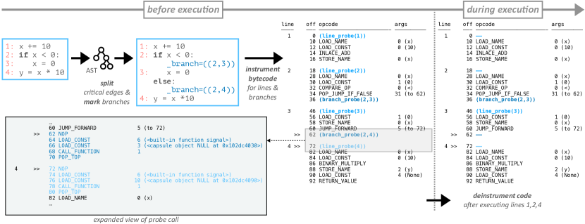
Figure 1. Overview: SlipCover drastically reduces overhead compared to the state-of-the-art tracing-based coverage analysis tool for Python (coverage.py) via a combination of three approaches: (1) AST transformation (Section 2.1), (2) lightweight bytecode instrumentation (Section 2.2), and (3) dynamic bytecode de-instrumentation (Section 2.3). AST transformations let SlipCover accurately identify all branches in the program source. Inserted bytecode instrumentation then tracks lines and branches at runtime. In code regions where lines or branches have been covered, SlipCover gradually rewrites their bytecode to eliminate instrumentation, letting the Python code subsequently run at full speed. Python bytecode varies with version. This paper uses Python 3.10 bytecode throughout.

1. Introduction

Code coverage analysis is widely used for a variety of tasks including testing, program analysis such as slicing, and statistical fault localization. Branch and line coverage information can reveal areas of code that are not exercised by a test suite. Automated testing approaches, like mutation testing and fuzzing, use coverage information to evaluate mutants or drive the exploration of new code paths.

Unfortunately, existing code coverage analyzers often substantially degrade performance (Chilakamarri and Elbaum, 2006). The source of this slowdown is primarily due to overhead that the dynamic analysis imposes to obtain the coverage information at execution time (Chilakamarri and Elbaum, 2006; Tikir and Hollingsworth, 2005). Code coverage analyzers typically either instrument each line of code, inserting probes that record when these are reached, or, in the case of Python, build on that language’s built-in tracing support. The slowdown imposed by code coverage analyzers has a significant impact not only on the time to run tests or the number of tests that can be run in a given time budget. At Google, “coverage instrumentation is relatively expensive, and performance failures are the most common cause of failed coverage computations” (Ivanković et al., 2019).

In the context of Python, which is already notoriously slow (Lion et al., 2022), coverage analysis leads to dramatic slowdowns. As Section 4 shows, the popular and widely used state-of-the-art code coverage analysis tool for Python, coverage.py (used at Google, with 7.4 million downloads per week) (Batchelder, 2023), increases execution times by between 30% and 260% (median: 180%) vs. CPython, the standard Python interpreter (CPython, 2023). This overhead is even more extreme when running PyPy, a JIT compiled implementation of Python (PyPy, 2023), slowing down programs by 140%–32,400% (median: 1,300%).

This paper presents SlipCover, a near-zero overhead coverage analysis approach for Python (CPython median: 5%). SlipCover first performs an AST transformation to accurately identify branches in the Python source code. It then inserts low-overhead instrumentation that tracks branch and line coverage at runtime. Critical to its efficiency, it gradually eliminates probes as lines or branches are covered, eventually letting code run at full speed. SlipCover manages the cost of de-instrumentation with its expected performance benefits, triggering de-instrumentation only once it crosses a cost-benefit threshold.

We show that SlipCover accurately collects coverage information while effectively eliminating the overhead of coverage analysis. SlipCover’s efficiency not only can drastically reduce time spent testing and expand the number of fuzzing, mutation tests, or unit tests in a given time budget. It also enables new use cases for coverage analysis: for example, because of its low overhead, SlipCover could be used in deployment to identify code that is never used by any client, and is thus suitable for removal (Tikir and Hollingsworth, 2005). In a proof of concept, we show the value of speeding coverage analysis in the context of a coverage-guided property-based testing system (DeVoe and Lampropoulos, 2023), where it yields a $22\times$ speedup.

This paper makes the following contributions:

• It presents SlipCover, a new line and branch coverage analyzer for Python based on AST transformation, bytecode instrumentation and de-instrumentation.

• It conducts a detailed empirical analysis of SlipCover, showing that it significantly advances the state of the art, almost completely eliminating the overhead of coverage analysis.

2. SlipCover Overview

Figure 1 presents a graphical overview of SlipCover. SlipCover operates in two phases: a static phase and a dynamic phase. The static phase, shown to the left of the dotted line, performs AST transformations (Section 2.1) and inserts probes as the Python interpreter loads code (Section 2.2). The dynamic phase tracks coverage and dynamically eliminates probes when they are no longer needed (Section 2.3).

The figure shows on the left a sample portion of Python code, followed by the results of SlipCover’s AST transformation and the resulting instrumented bytecode. On the right, it shows the same bytecode after SlipCover has partially de-instrumented it.

2.1. AST Transformation

SlipCover’s static phase begins with AST transformations to split critical edges in the control flow graph and to mark branches. Critical edges result from statements that are optional or empty. As an example, Figure 2 shows a code excerpt containing an if statement without a matching else, and Figure 3 the resulting control flow graph.

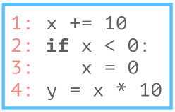
Figure 2. Example: An if statement is used without a matching else.

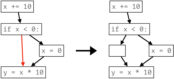
Figure 3. Critical Edge: SlipCover transforms the code example’s AST, spliting a critical edge (shown in red) to facilitate efficient instrumentation.

Branch coverage analysis requires that the system record whether any branch was taken, even if one of them is implicit. Splitting these edges lets SlipCover perform branch coverage analysis accurately and efficiently using bytecode instrumentation. SlipCover parses the code and transforms the resulting abstract syntax tree to add explicit branches for these cases. To simplify this transformation, SlipCover leverages an idiosyncrasy of Python, which has explicit else statements not only for if but also for most control flow constructs (e.g., while and for).

SlipCover then marks the branches, inserting placeholder assignments which the instrumentation step replaces with probe calls. Figure 4 shows the resulting transformation.

2.2. Bytecode instrumentation

The final step in the static phase performs bytecode instrumentation. SlipCover uses source line information and any branch placeholders to guide the insertion of probes in the code. The probes perform three roles: (1) they mark the relevant line or branch “covered”, (2) they track the number of times they execute, and (3) they trigger de-instrumentation once that counter crosses a threshold.

SlipCover’s probes consist of two parts: a C++ extension module, and bytecode sequences (shown in expanded view in Figure 1) that call into that module. This two-pronged approach has two benefits. First, placing most of the probe functionality in a native extension module helps keep the probes lightweight, avoiding Python interpreter overhead and leveraging Python’s efficient integration with native code. Second, instrumenting the bytecode to call into it lets SlipCover avoid having to modify the interpreter. As Section 3.3 describes, this approach also helps keep de-instrumentation efficient.

2.3. Program execution and dynamic de-instrumentation

Once SlipCover finishes instrumenting the program, it initiates program execution, marking the beginning of the dynamic phase. If the program imports (loads) additional code during execution, SlipCover suspends the dynamic phase, performs its static phase steps on the new code, and then resumes execution.

Now, as the program being executed reaches each line and branch for the first time, it first executes the inserted probe. The first time a probe is executed, it records the line or branch as being covered, which implicitly marks the probe as eligible for eventual elimination (rather than immediately eliminating it, for reasons discussed in the next paragraph). Subsequent executions of the probe only increment a counter and check to see if it crosses a predefined threshold count. Upon crossing that threshold, the probe triggers elimination of all marked probes.

Delaying de-instrumentation makes SlipCover more efficient. Bytecode modifications are relatively expensive, and batching de-instrumentation amortizes this overhead. This approach also lets SlipCover limit de-instrumentation costs for rarely executed code, whose probe cost yields limited overhead. If probes execute often, more are eliminated, but if they only execute once, or even a few times, no time is wasted eliminating them.

3. SlipCover Implementation

This section describes key portions of SlipCover’s implementation in detail, including its AST transformation for branch coverage (Section 3.1), probe insertion (Section 3.2), probe elimination (Section 3.3), and code loading interception (Section 3.4).

3.1. Instrumenting for Branch Coverage

As Section 2 describes, the first step in SlipCover’s static phase performs AST transformations to identify the branches in the code. As an alternative, we considered performing control-flow analysis on the bytecode, identifying branches through jump instructions and their source and destination lines. One advantage of this approach would have been that SlipCover would be able to operate without source code. While Python code is generally distributed in source form, the bytecode can be executed without accompanying source code.

Unfortunately, this approach is unworkable. Python’s bytecode compiler performs transformations that make the correspondence between jump instructions and their branches in the source code difficult if not impossible to identify. This challenge was first identified for coverage tools that rely exclusively on Java bytecode by Li et al. (2013), who found that the exclusive reliance on bytecode leads to inaccurate branch coverage analysis.

Instead, SlipCover employs a hybrid approach to collecting branch coverage. It uses Python’s compiler and ast library to parse Python source into an AST. It then transforms the AST, splitting critical edges (see Figure 3) and demarcating all branches by injecting assignment statements into the code that encode the origin and destination lines of each branch (e.g., _branch = (origin, dest)). Unlike branches, assignment statements are straightforward to recognize in generated bytecode. Figure 4 shows this transformation for an if statement.

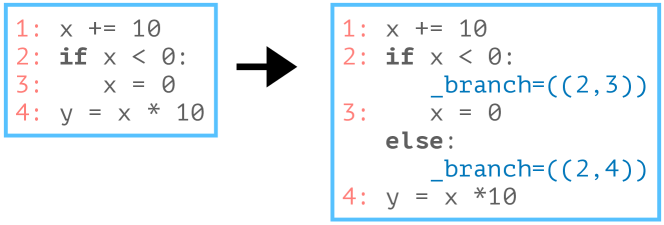
Figure 4. Demarcating branches: SlipCover inserts assignment statements to demarcate branches.

SlipCover’s AST transformation pass splits critical edges, making all branches explicit. It leverages an idiosyncrasy of Python that simplifies this AST transformation. Unlike other widely-used programming languages, Python’s else statement not only combines with if, but also with for and while statements. In these cases, the else branch is executed when the conditional evaluates to False. To make all branches explicit, SlipCover simply inserts an else statement, when missing, after all ifs and for and while loops. Figure 5 shows an example of this transformation.

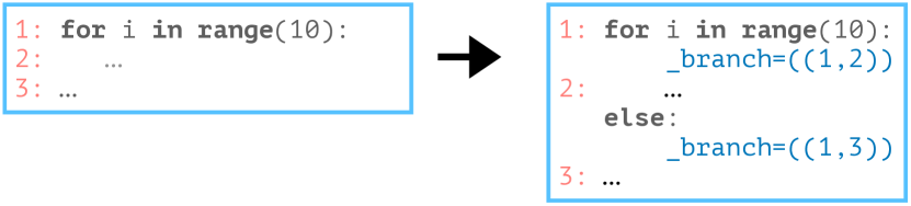
Figure 5. Demarcating loop branches: Unusually, Python allows the use of else with for and while statements, simplifying inserting code to demarcate the block skipping branch ($1\rightarrow 3$ in the example).

Python 3.10 introduced match statements (Python match statement, 2023), which are structurally similar to the well-known C switch statement. While match cannot be combined with else, its wildcard case _: statement can be used similarly. Figure 6 shows an example.

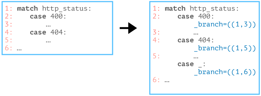
Figure 6. Demarcating match: SlipCover inserts a “match _” statement, if missing, to demarcate that branch.

Having performed these modifications, SlipCover then compiles the AST into bytecode. The next step in the static phase replaces the demarcations with branch probes.

3.2. Inserting Probes

The second and last step in SlipCover’s static phase insert probes into the bytecode. This step also reads from a bytecode object, which is either the one compiled from the AST in the first static step, or the unmodified bytecode loaded from Python, if no branch coverage is being collected. Python bytecode objects include metadata indicating the source code file and line corresponding to each portion of code. SlipCover uses this information to determine where to insert its line probes. SlipCover scans the code for the special _branch assignments introduced in the first step (Section 3.1). As Figure 7 shows, SlipCover inserts probes ahead of the code for each line and branch.

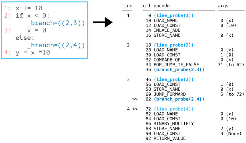
Figure 7. Inserting Probes: SlipCover inserts line and branch probes guided by Python metadata and its own branch demarcations. For clarity, line_probe($l$) and branch_probe(($l_{1},l_{2}$)) stand for the actual probe bytecode sequences (see Figure 8).

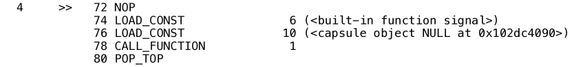
Figure 8. Probe bytecode: line_probe(4) sequence from Figure 7. SlipCover replaces the NOP opcode with a JUMP_FORWARD to skip over the entire sequence when eliminating the probe.

Figure 8 presents an actual probe bytecode sequence. These start with a NOP opcode that SlipCover later may replace with a JUMP_FORWARD to skip over (eliminate) the probe sequence (see Section 3.3). The rest of the sequence invokes the native portion of the probe, which is wrapped in a Python “capsule” object. SlipCover instantiates a new capsule object for each line and branch probe as it inserts them. Since their addresses are known at insertion time, SlipCover stores all addresses as code constants, avoiding the need to perform costly lookups during execution.

The native portion of the probe implements the rest of the probe logic. It records the newly covered line or branch when it is first executed, and triggers de-instrumentation once it has executed a certain number of times (Section 3.3).

Modifying Python bytecode is one of the more intricate parts of SlipCover. Since Python bytecode objects are read-only, SlipCover must create new objects to insert probes. Python opcodes also have variable length. The base form is just one byte for the opcode and one for the argument, but it may also be preceded by up to three EXTENDED_ARG opcodes if the argument is longer than one byte. Figure 9 shows an example.

Figure 9. Extended arguments: Python uses a special EXTENDED_ARG opcode to encode multi-byte arguments (a jump forward to 0x01020304 in this case).

SlipCover inserts probes by shifting the original bytecode down at each insertion point. As it does so, it updates existing jump destinations and various metadata, including the line table and the exception handler table. Unfortunately, inserting bytecode may also increase the offset (or difference in offset, for relative jumps) between jump opcodes and their destinations. If the new destination then does not fit in the space occupied by the original jump, SlipCover may need to insert additional EXTENDED_ARG opcodes. Inserting EXTENDED_ARGs may require updating the jumps again. SlipCover deals with this issue via the same approach as the CPython compiler: it repeatedly updates jumps as long as any length adjustments are necessary.

It might seem possible to adapt a design similar to that employed by Tikir and Hollingsworth (2005) in order to reduce instrumentation overhead. Adapting their approach would involve replacing the bytecode at each insertion point by a jump to a trampoline section of bytecode. This trampoline would be allocated at the end of the original code. It would first call to the native probe, then execute the bytecode that was replaced, and finally jump back to the original code right after the insertion point. By avoiding bytecode shifts, this approach theoretically offers the promise of reducing probe insertion overhead. Moreover, it would also would have made it possible to efficiently fully remove probes by restoring the original bytecode, overwriting the jump to the trampoline.

Unfortunately, that approach is not viable in the context of Python. A jump to a trampoline would not necessarily fit in the space between two insertion points. For example, a line of Python code, when compiled, might yield only two bytes: an opcode and its argument. Code for the next line would then start at the third byte. If a jump to the trampoline required four or more bytes (a likely scenario), there would be no room to insert it without corrupting the following line’s bytecode.

3.3. Eliminating Probes

SlipCover structures its probes so that it can eliminate probe overhead during de-instrumentation in a streamlined manner, as this section describes.

SlipCover records coverage in two sets: a “known” set and a “newly covered” set. The first time a probe executes, it adds coverage information (e.g., this line is now covered) to the newly covered set, which also indicates that the probe is ready for elimination.

The first step in SlipCover’s de-instrumentation is to set a flag in the probe that indicates it should skip recording coverage information in subsequent executions. This flag avoids much of the overhead of instrumentation (adding to covered sets). Subsequent executions only perform that check and then increment an execution counter. Once the execution counter crosses a pre-defined threshold, it performs the final de-instrumentation step, eliminating any previously reached probes.

SlipCover then atomically swaps the “newly covered” for a new, empty set, where any additional coverage is recorded while it processes the items previously in “newly covered”. It adds these items to the “known” set and then uses maps it created during instrumentation to efficiently locate the bytecode objects containing their respective probes.

As Section 3.2 describes, modifying bytecode can be a complex operation. To simplify and save time during probe elimination, SlipCover does not delete the probe sequences from bytecode. Instead, it inserts a jump over them, effectively removing the probe without the complexity entailed by actually deleting the code (including updating line numbers and jumps).

SlipCover leverages another idiosyncratic behavior of Python to simplify this operation. SlipCover’s probes start with a NOP opcode. All opcodes in Python are encoded with an argument, including NOP, whose argument Python ignores. SlipCover exploits this encoding to pre-encode the length of the probe sequence into NOP’s argument. To eliminate a probe, SlipCover then simply replaces that NOP with a JUMP_FORWARD opcode.

Since Python bytecode objects are read-only, SlipCover creates new instances for any objects with newly eliminated probes. Bytecode objects are also tree-structured, as any nested functions, lambda functions, or comprehensions are included as constants in the enclosing bytecode object.

Consequently, to eliminate probes, SlipCover performs a depth-first search of the applicable bytecode objects, replacing these bytecode “constants” as it moves from a child node to a parent node. Python stores additional references to bytecode objects in dictionaries that it uses to implement its various variable contexts. Once all covered probes have been eliminated, SlipCover searches for any such references, replacing them with the new instances. SlipCover’s search is comprehensive, including all modules it has instrumented, as well as every Python frame’s global and local contexts. Such updates are most efficiently performed in batches to reduce the frequency of searches. This fact in part motivates SlipCover’s threshold-based de-instrumentation.

SlipCover thus gradually de-instruments the program as it executes, allowing it to continue to run at close to full speed, while leaving as-yet unreached probes in place to record coverage should an execution path reach them.

3.4. Intercepting Code Loading

In order to instrument bytecode, SlipCover must intercept code as the Python interpreter loads it, which can happen at any time during execution. It performs this task by inserting its own specialization of importlib’s MetaPathFinder at the head of Python’s import path. This approach lets SlipCover observe and interpose on all subsequent module load requests. To reduce overhead, SlipCover does not instrument every module, but only that are deemed relevant (either by a default set, or those specifically specified by the user).

One complication is that the widely-used testing framework pytest also inserts its own Loader, which it uses to modify unit tests in order to better support assert statements. That loader would normally bypass SlipCover’s, causing unit tests to be excluded from the coverage measurement. To avoid that, SlipCover preloads pytest’s assertion rewriter and “monkey patches” it, interposing itself so it can instrument the unit tests while still allowing pytest to later make its own changes.

4. Evaluation

Our evaluation answers the following research questions:

• RQ1: How does SlipCover’s performance compare to the state-of-the-art (coverage.py) (Section 4.2)?

• RQ2: How much does SlipCover’s de-instrumentation contribute to its high performance (Section 4.3)?

• RQ3: How does SlipCover’s approach behave across recent Python versions (Section 4.4)?

• RQ4: What is the overhead of approaches based on Python’s tracing mechanism, as used by coverage.py (Section 4.5)?

• RQ5: What is the impact of de-instrumentation when running in the PyPy JIT compiler (Section 4.6)?

• RQ6: How does SlipCover affect the performance of automated testing frameworks (Section 4.7)?

4.1. Experimental Setup

We perform all experiments on a 10-core 3.70GHz Intel Core i9-10900X system equipped with 64GB of RAM and an NVIDIA GeForce RTX 2080 SUPER GPU, running Linux 5.16.19-76051619-generic. We compile SlipCover’s C++ code as well as the various CPython interpreter versions with GCC 9.4.0, utilizing Python’s default flags, which include -O3 optimization. We utilize the stock PyPy 3.9-v7.3.11 distribution from pypy.org. Except where noted otherwise, we use CPython 3.10.5 and coverage.py 6.4.4. We perform all measurements on an otherwise quiescent system. All measurements are taken five times, and we report the median.

We select as benchmarks a mix of test suites for real-world applications, as well as compute-intensive Python applications. The benchmarks include the test suites for the scikit-learn (Pedregosa et al., 2011) and Flask (et al., 2023) packages, both “real world” users of coverage analysis, selected for relevance as well as for their range of running times. Scikit-learn’s suite runs for about ten minutes (using CPython) and is representative of a long-running suite. Flask’s less comprehensive suite, whose runtime we extend by utilizing the pytest-repeat package to repeat the tests five times, runs for less than ten seconds. We also include several pure Python applications: fannkuch, mdp, pprint, raytrace, scimark and spectral_norm, the longest-running benchmarks in the standard Python Benchmark Suite used to evaluate Python performance (The Python Benchmark Suite, 2023), and Peter Norvig’s Sudoku solver (Norvig, 2010), a compute-intensive pure Python application.

4.2. [RQ1] How does SlipCover’s performance compare to coverage.py?

We compare SlipCover’s and coverage.py’s performance by using these to analyze coverage on our benchmark suite. We normalize results against their base running time, i.e., running without any coverage analysis.

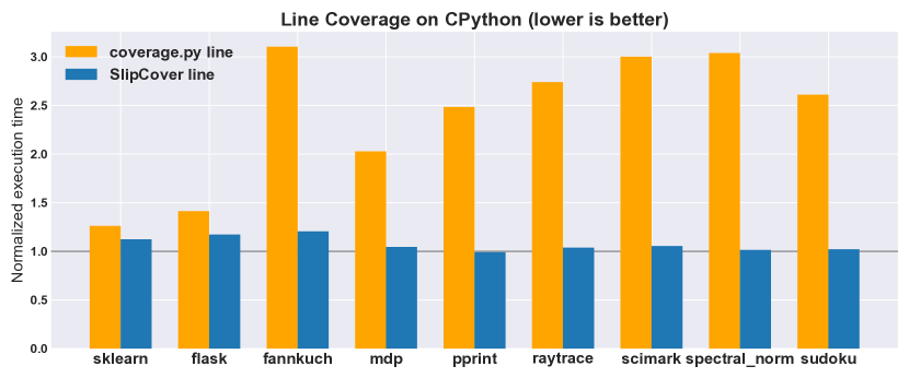
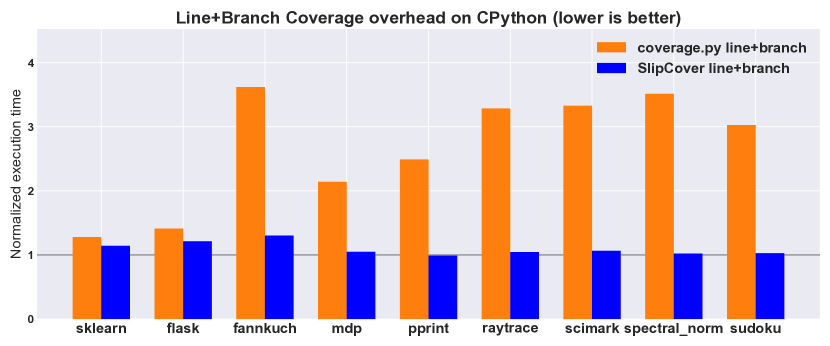
Figure 10. [RQ1] SlipCover is much faster than the state of the art (coverage.py) on CPython: across our benchmark suite, while coverage.py incurs up to 260% overhead, SlipCover’s median overhead remains at 5%.

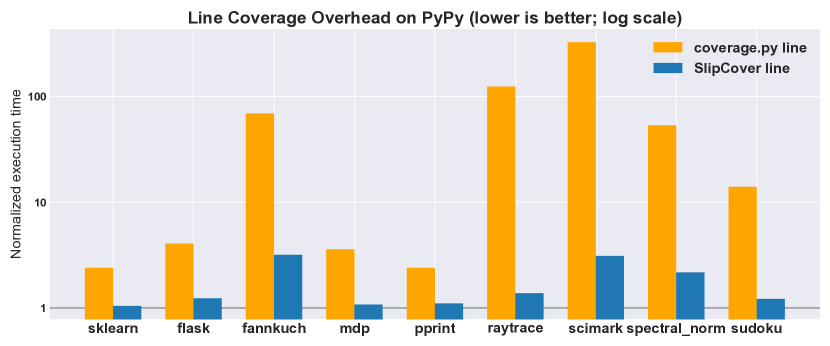
Figure 11. [RQ1] SlipCover is also much faster than coverage.py on PyPy: while coverage.py incurs up to 32,470% overhead, SlipCover’s median overhead remains at 23%.

Figures 10 and 11 present the results of this comparison. In Figure 10, while coverage.py increases execution times by between 30% and 260% (median: 140%), SlipCover’s overhead remains at or below 21% (median: 5%). In Figure 11, while coverage.py increases execution by between 140% and 32,470% (median: 140%), SlipCover’s overhead remains at or below 220% (median: 23%). PyPy’s JIT speeds up the raytrace and scimark benchmarks especially well, leading to short execution times without coverage analysis. This leads to coverage.py showing an extreme performance overhead, as the denominator normalizing that execution is very small. Summary: SlipCover is much faster than coverage.py on both CPython and PyPy.

4.3. [RQ2] How much does de-instrumentation contribute?

As Section 3.3 describes, SlipCover de-instruments code in two steps: (1) immediately after recording new coverage, each probe sets a flag indicating it need not record it again, and (2) each time a probe is reached, it increments a counter and eliminates all covered probes when it crosses a threshold. To quantify the effect of each de-instrumentation step, we measure SlipCover’s performance while (a) disabling the probe elimination, the second step described above, and (b) disabling de-instrumentation entirely (both steps).

Figure 12 shows that simply replacing Python tracing with code instrumentation does not achieve the performance gains yielded by de-instrumentation. On the other hand, de-instrumentation is most beneficial to programs that re-execute previously covered paths, such fannkuch and those on the right of the figure. The figure also shows that most of the de-instrumentation overhead is eliminated in step (1). Summary: De-instrumentation is key to reducing SlipCover’s overhead.

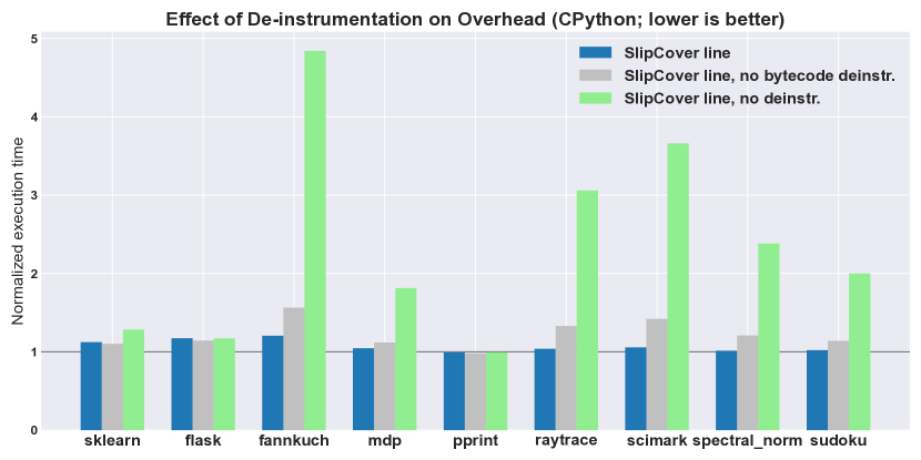
Figure 12. [RQ2] De-instrumentation is key to SlipCover’s performance: Comparing SlipCover’s normal execution time (blue), to partial de-instrumentation (grey) and to no de-instrumentation (green) demonstrates the importance of de-instrumentation in reducing SlipCover’s overhead.

4.4. [RQ3] How does SlipCover’s approach behave across Python versions?

Python is currently the subject of efforts to increase its performance (Faster CPython, 2023; Shannon, 2021). It is a natural question to ask how these efforts might impact the relative performance of SlipCover and coverage.py. If the trends show a narrowing gap, then the long-term benefit of SlipCover would be unclear.

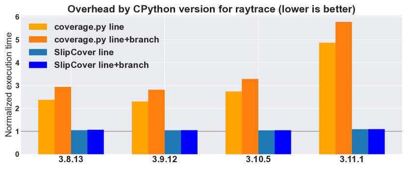
Figure 13. [RQ3] coverage.py’s relative overhead is growing with successive Python versions, while SlipCover’s overhead remains near zero. As Python developers improve the speed of Python, the added overhead of coverage.py consumes an increasingly large portion of execution time.

Figure 13 compares coverage.py’s and SlipCover’s execution times relative to the uninstrumented base case, without coverage analysis, for four CPython versions, from 3.8 to 3.11. To simplify the figure, we include only one benchmark, raytrace.

As the graph shows, coverage.py’s performance suffers slightly in CPython 3.10, and more pronouncedly in CPython 3.11.1 despite developer’s efforts (Python 3.11 tracing performance degradation, 2022). In fact, since execution times are normalized by the time without coverage analysis, any improvement in Python’s performance reduces the denominator, relatively increasing coverage.py’s overhead. Summary: SlipCover’s overhead is near zero across Python versions, while coverage.py’s overhead is growing over time.

4.5. [RQ4] What is the overhead of approaches based on Python’s tracing mechanism (as used by coverage.py)?

To investigate whether a new approach to collecting coverage information is necessary, we create a “null” tracer. Like the one employed by coverage.py, our null tracer registers a tracing callback using Python’s C API (Python C tracing API, 2023). It also attempts to avoid unnecessary overhead by dynamically turning tracing off for functions whose coverage information is irrelevant. These are typically Python library functions, but test suite developers also commonly specify directories containing relevant code. The null tracer does not, however, record any lines or branches, or perform any complicated checks. Its dynamic tracing control only checks the source file path prefix.

Figure 14 shows the null tracer’s relative running times next to coverage.py’s. The null tracer’s overhead ranges between 42% and 99% (median: 63%) of coverage.py’s overhead. Summary: tracing is expensive, and comprises much of the cost of coverage.py.

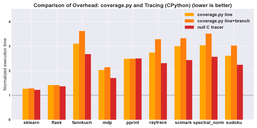
Figure 14. [RQ4] Tracing accounts for much of the execution time overhead of coverage.py: the relatively large overhead incurred by the “null” tracer ($\S$4.5) strongly suggests that much of coverage.py’s running time is, in fact, due to tracing.

4.6. [RQ5]: What is the impact of de-instrumentation when running in the PyPy JIT compiler?

The effective de-instrumentation we observe through the Java JIT compiler optimizations (Section 5) raises the question whether SlipCover’s de-instrumentation is still relevant in the context of PyPy, a JIT compiler for Python. To answer this question, we compare the overhead of SlipCover’s coverage analysis to its overhead if all de-instrumentation is disabled. Figure 15 shows the results. While de-instrumentation does not significantly improve performance for all benchmarks, it dramatically reduces overhead for several. Summary: de-instrumentation has a dramatic impact on performance when running with PyPy’s JIT compiler, reducing overhead by $40\times$–$150\times$.

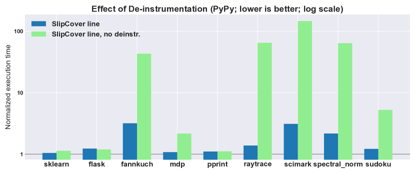
Figure 15. [RQ5] De-instrumentation on PyPy: de-instrumentation is vital for SlipCover’s performance for some benchmarks on PyPy, despite its JIT compiler.

4.7. [RQ6]: How does SlipCover affect the performance of automated testing frameworks?

As a proof of concept, we utilize an example program from TPBT (DeVoe and Lampropoulos, 2023), a property-based testing system, that originally draws coverage information from coverage.py to guide the testing. We create an alternative version that measures coverage using SlipCover and compare their running times. We observe that with SlipCover, the program runs in 1s, about 22$\times$ faster than the 22.3s it runs in when drawing coverage information from coverage.py. Summary: SlipCover can greatly improve the performance of coverage-guided testing.

5. Other Programming Languages

Many of the techniques SlipCover demonstrates in the context of Python should be applicable to other bytecode-based languages. These may naturally require some adaptation depending on what is available or efficient in the language and execution environment. While evaluating this in detail goes beyond the scope of this paper, we explore the question of applicability to other programming languages by creating and evaluating a proof-of-concept version of SlipCover for Java.

Prior work for Java (Chilakamarri and Elbaum, 2006) required changes to the JVM because at the time no API was available to allow bytecode modification at runtime; we instead utilize the Java Instrumentation API (Java Instrumentation, 2023).

De-instrumentation cost

When on-stack bytecode replacement is not supported by the interpreter, de-instrumenting it incurs a larger cost. In Python, such cost stems from replacing the bytecode object and updating references to it (Section 3.3). In Java, the Instrumentation API requires the modified bytecode to be passed in class file format. The cost then stems from recreating the entire class containing the changed bytecode, as well as loading and eventually JIT-recompiling it.

In such situations, it becomes important to manage these costs, only de-instrumenting bytecode that seems likely to execute again. While SlipCover’s simple per-probe threshold proved effective for Python, initial data for Java suggests that modifying the mechanism to a per-method or per-class threshold might better balance de-instrumentation gains and costs given that the Instrumentation API modifies an entire class at once.

Lightweight probes

A probe might execute multiple times until its de-instrumentation is triggered and the replacement bytecode is used. For that reason, it is important to keep probes lightweight, that is, incurring as low overhead as possible. SlipCover’s Python probes were designed as a bytecode and native hybrid because in Python (and especially in CPython, where all execution is interpreted), using native code is crucial to performance. In Java, our prototype utilizes static boolean arrays and method-local variables created during instrumentation to keep overhead as low as possible.

Optimizing JIT compilers

We compare the prototype’s running time with that of a popular Java coverage analyzer, JaCoCo (JaCoCo Java Code Coverage Library, 2023). We discover to our surprise that JaCoCo’s performance rivals and in certain cases even exceeds the prototype’s performance.

To investigate why, we instrument a small Java program with JaCoCo. Figure 16 shows the program, which contains a loop that repeatedly divides a variable by a constant (line 5) and adds a constant to it (line 6).

⬇

1 class T {

2 static void foo() {

3 double n = 0.2;

4 for (int i=0; i<100000; i++) {

5 n /= 1.1;

6 n += .1;

7 }

8 System.out.println("n=" + n);

9 }

10

11 public static void main(String... args) {

12 foo();

13 }

14 }

Figure 16. Sample Java program: we instrument this program with JaCoCo and review the native code emitted by the JVM’s JIT compiler to understand how JaCoCo achieves high performance despite not performing de-instrumentation.

Figure 17 shows a portion of the resulting Java bytecode, highlighting the JaCoCo instrumentation. JaCoCo records coverage by creating a Boolean array where each element corresponds to a portion of the code. Bytecode offsets 0–5 in Figure 17 provide access to that array. JaCoCo also inserts various probes into bytecode that set elements in the array to true as they execute. Bytecode offsets 12–15 contain such a probe.

⬇

0: ldc #65 // Dynamic #1: jacocoData:Ljava/lang/Object; 2:\textbf{checkcast}\textbf{\#67}// class "[Z" 5:\textbf{astore\_0}6: ldc2_w #7 9: dstore_1 10: iconst_0 11: istore_3 12:\textbf{aload\_0}13:\textbf{iconst\_1}14:\textbf{iconst\_1}15:\textbf{bastore}

16: iload_3

17: ldc #9

19: if_icmpge 44

[...]

Figure 17. JaCoCo instrumented bytecode: This bytecode results from compiling the sample program in Figure 16 and instrumenting it with JaCoCo. At the beginning of the method, JaCoCo creates a Boolean array to record coverage. It also inserts probes that set array elements to true.

After instrumenting the program, we execute it by invoking the JVM using the following flags:-XX:+UnlockDiagnosticVMOptions -XX:CompileCommand=print,T.foo. which logs native code produced by its JIT compiler, if any.

Figure 18 shows a portion of the x64 code logged by the JVM. At the top of the listing, a movb instruction stores the value 1. That corresponds to assigning true to an element of JaCoCo’s coverage Boolean array. The vdivsd and vaddsd instructions implement the division and addition operations from source code lines 5 and 6.

The JIT compiler thus optimized the loop, unrolling it, and also hoisted any Boolean assignments out of it. The loop consists exclusively of the arithmetic instructions already mentioned, followed by an iteration counter update (adding 0x10 at a time, as the loop was unrolled to perform 16 operations without further checking).

⬇

=================== C2-compiled method ====================

[...]

0x00007f198d1825f5: movb  0x1,0x12([...] 0x00007f198d182630: vdivsd -0x118(0x00007f198d182638: vaddsd -0x118(0x00007f198d182640: vdivsd -0x128(0x00007f198d182648: vaddsd -0x128(0x00007f198d182650: vdivsd -0x138(0x00007f198d182658: vaddsd -0x138([...] 0x00007f198d182720: vdivsd -0x208(0x00007f198d182728: vaddsd -0x208(0x00007f198d182730: add\0x10,%ebp

0x00007f198d182733: cmp %r10d,%ebp

0x00007f198d182736: jl 0x00007f198d182630

[...]

Figure 18. JIT generated code omits instrumentation: Java’s C2 JIT compiler generated this x64 code, unrolling the sample program’s loop and omitting (hoisting) the movb instructions used to record coverage from it.

The result is that in modern implementations of Java, the optimizing JIT compiler eliminates much of the overhead of probes, even without de-instrumentation. The limited remaining performance gap does not justify the effort of producing a full port of SlipCover to Java.

Section 4.6 shows that the same situation does not apply to Python. When running with the PyPy JIT, not de-instrumenting can in some cases degrade performance dramatically, slowing execution by $40\times$–$150\times$.

6. Prior Work

This section describes previous work aimed at reducing the overhead of coverage analysis. Section 6.1 first describes approaches that instrument code only statically (entirely prior to execution time). Section 6.2 describes approaches that (also) modify code dynamically (during execution). Section 6.3 compares SlipCover’s design, algorithms and implementations with past approaches. Finally, Section 6.4 details coverage.py, the current state-of-the-art profiler for Python.

6.1. Static instrumentation

Java

As far as we are aware, Pavlopoulou and Young (1999) are the first to propose removing instrumentation once coverage is recorded. Their approach, which the paper calls “residual” test coverage, is to instrument bytecode in Java class files to record when each basic block is reached, skipping those that a previously-instrumented execution had reached (each execution updates the class files on disk). It works with stock (unmodified) JVMs but is only able to de-instrument code the next time the program executes.

Native code

Nagy and Hicks (2019) present a similar approach for use in fuzzing called “full speed fuzzing.” It performs binary instrumentation to trigger software interrupts whenever basic blocks are reached for the first time. It rewrites the binary on disk to de-instrument that basic block, and then re-executes the binary to continue fuzzing.

6.2. Dynamic instrumentation

Native code

Tikir and Hollingsworth (2005) implement a code coverage analyzer by extending DyninstAPI (Buck and Hollingsworth, 2000), a library for dynamic native code instrumentation. It is the earliest work to both dynamically insert and remove coverage probes during program execution. It is limited to line coverage. To reduce the initial overhead of instrumentation, it performs control-flow dominator based static analysis on the code and only places probes in certain basic blocks. It implements both pre-instrumentation, which inserts all probes ahead of time, and on-demand instrumentation, which inserts breakpoints at the beginning of functions to perform the required analysis and then insert probes when a function is executed. Finally, it periodically (at fixed time intervals) removes probes that are no longer needed.

Java

Chilakamarri and Elbaum (2006) proposes a similar “disposable” coverage instrumentation for Java. It instruments JVM bytecode and, once a probe is no longer needed, de-instrument it by overwriting the probe with NOP operations. It requires modifications to the JVM to trigger de-instrumentation of both interpreted and JIT-compiled bytecode. We note that it might be possible today to accomplish this via the Java Instrumentation API (Java Instrumentation, 2023), which was not available at that time. Section 5 presents an evaluation of a prototype using this approach.

Another Java-based approach, Misurda et al. (2005) implements both dynamic probe insertion and removal. In the same vein as Tikir and Hollingsworth (2005), it only pre-instruments by inserting seed probes which further instrument basic blocks once reached. Its approach is to instrument the x86 code generated by the JIT compiler, relying on support provided by Jikes, a research virtual machine. This approach would be unsound in modern, industrial-strength JVM implementations, which initially interpret bytecode.

Surprisingly, as Section 5 shows, the optimizations that modern Java JIT compilers perform eliminate most of the overhead of instrumented code, yielding few opportunities to gain performance by de-instrumentation in the context of Java.

6.3. Comparisons with SlipCover

This section characterizes the differences with prior work by contrasting SlipCover’s algorithmic and technical approaches.

On-the-fly de-instrumentation

While Python does not require compilation into bytecode ahead of time, it caches previous compilations in .pyc files as a way to speed up program startup. While it would be possible to adapt the above-described approaches to Python bytecodes, it would still delay all de-instrumentation until a subsequent execution (if any). By contrast, SlipCover de-instruments code live, immediately speeding the current program execution.

Aggressive vs. optimized probe insertion

SlipCover does not attempt to reduce the number of probes inserted, but instead adds probes for every line and branch ahead of program execution. SlipCover adopts this design decision based on the observation of (Tikir and Hollingsworth, 2005): “the most significant gains come from removing instrumentation code […] rather than from binary analysis algorithms to optimize instrumentation placement.” In fact, such an approach that adds bytecode probes on demand would be difficult to adapt to Python, as bytecode objects are read-only.

Beyond that technical issue, the approach of attempting to avoid overhead a priori is complicated by the fact that in Python, many opcodes can result in a branch by throwing an exception. The result would be basic blocks consisting of few or even just a single opcode.

Stepwise de-instrumentation

As Section 3.3 describes, SlipCover reduces probe overhead in two steps: one immediately once the probe is no longer needed, and another threshold-based, thus amortizing the cost of de-instrumentation. By contrast, Tikir and Hollingsworth (2005)’s approach only removes probes at fixed time intervals, which may be either too aggressive or too lazy.

Overwriting a probe with NOP operations (Chilakamarri and Elbaum, 2006) is convenient for Java because it does not require updating any bytecode metadata. If a Java application were to add a jump opcode, it would need to update the bytecode’s StackMapTable (Lindholm et al., 2013), a more complex operation. Python does not have the same restriction, so SlipCover’s second de-instrumentation step uses a jump opcode to effectively remove probes.

No modifications to VMs

SlipCover executes on unmodified Python interpreters. Approaches like Chilakamarri and Elbaum (2006) that require modifying the VM are undesirable in many settings: a modified Python interpreter or JIT would require separate installation and likely hamper adoption.

Portable and complete instrumentation

While operating at the x86 level lets Misurda et al. (2005) benefit from efficient code manipulation (while sacrificing portability to non-x86 platforms), it also makes its approach generally unsuitable for Python. Despite exceptions such as native extension modules and compiled Python variants, Python typically is interpreted (entirely in CPython, and initially in PyPy). Misurda et al. (2005)’s approach would also be unsound in any modern Java implementation, which only JIT-compile code once the interpreter has executed the bytecode long enough to identify its hot spots. By contrast, SlipCover ensures complete coverage of all Python byte code.

6.4. Comparison with coverage.py

coverage.py (Batchelder, 2023) is the standard coverage analysis tool for Python. It uses Python’s profiling and tracing API (Python C tracing API, 2023) to collect dynamic coverage information, registering tracer functions that Python invokes whenever it reaches a line. Section 4.5 shows that using this API introduces significant overhead, accounting for much of the coverage.py’s high overhead. SlipCover’s use of bytecode instrumentation and de-instrumentation avoids this overhead.

coverage.py collects strictly less information than SlipCover. Rather than performing line coverage, coverage.py performs statement coverage. Python statements can easily span multiple lines, including whenever there is an unclosed bracket or parenthesis, or by placing backslashes at the end of each line. coverage.py performs a pre-processing stage that omits continued lines when computing the set of all lines in the source.

For example, coverage.py does not report line 5 as not covered in the code below. By contrast, SlipCover correctly indicates that line 5 is not covered.

⬇

1 cond = True

2 foo = {

3 "const": 42,

4 "computed": 666 if cond \

5 else 999,

6 "other": 0

7 }

An analogous problem arises with branch coverage. coverage.py detects branches by recording arcs, which are line transitions it observes as the program execution moves from one line to another. Unfortunately, this method prevents coverage.py from detecting same-line branches. Consider the following code:

⬇

if x > 0: print("positive")

Because coverage.py sees no line transitions, it incorrectly does not detect the branch in this code. Unlike coverage.py, SlipCover’s AST-based instrumentation allows it to correctly detect all branches.

7. Conclusion

This paper presents SlipCover, a novel coverage analyzer that employs a combination of AST transformations and dynamic bytecode instrumentation and de-instrumentation to reduce the cost of collecting branch and line coverage information. SlipCover works with both the Python interpreter and PyPy, without modifications. It shows that bytecode de-instrumentation can be effective in industrial-strength language implementations, even when on-stack bytecode replacement is not supported.

Compared to coverage.py, the state-of-the-art Python coverage analyzer, SlipCover reduces overhead from 30%–260% to 5% when running with the Python interpreter, and from 140%–32,400% to 23% when running with PyPy. Using SlipCover can speed up coverage-guided testing by 22$\times$. SlipCover has been released as open source at https://github.com/plasma-umass/slipcover.

Appendix A Evaluation Data

This appendix shows the evaluation data from Section 4.

Table 1. [RQ1] Data for Figure 10, showing each benchmark’s execution time without coverage analysis, with line and line+branch coverage analysis by both coverage.py and SlipCover running on CPython.

Benchmark	no coverage	coverage.py line	coverage.py line+branch	SlipCover line	SlipCover line+branch
sklearn	$527.8\text{\,}\mathrm{s}$	$666.1\text{\,}\mathrm{s}$	$675.0\text{\,}\mathrm{s}$	$592.8\text{\,}\mathrm{s}$	$603.3\text{\,}\mathrm{s}$
flask	$8.0\text{\,}\mathrm{s}$	$11.3\text{\,}\mathrm{s}$	$11.3\text{\,}\mathrm{s}$	$9.4\text{\,}\mathrm{s}$	$9.7\text{\,}\mathrm{s}$
fannkuch	$15.1\text{\,}\mathrm{s}$	$46.9\text{\,}\mathrm{s}$	$54.6\text{\,}\mathrm{s}$	$18.2\text{\,}\mathrm{s}$	$19.7\text{\,}\mathrm{s}$
mdp	$10.4\text{\,}\mathrm{s}$	$21.1\text{\,}\mathrm{s}$	$22.3\text{\,}\mathrm{s}$	$10.9\text{\,}\mathrm{s}$	$10.9\text{\,}\mathrm{s}$
pprint	$13.0\text{\,}\mathrm{s}$	$32.3\text{\,}\mathrm{s}$	$32.4\text{\,}\mathrm{s}$	$12.9\text{\,}\mathrm{s}$	$12.9\text{\,}\mathrm{s}$
raytrace	$9.5\text{\,}\mathrm{s}$	$26.1\text{\,}\mathrm{s}$	$31.2\text{\,}\mathrm{s}$	$9.9\text{\,}\mathrm{s}$	$9.9\text{\,}\mathrm{s}$
scimark	$8.2\text{\,}\mathrm{s}$	$24.5\text{\,}\mathrm{s}$	$27.1\text{\,}\mathrm{s}$	$8.6\text{\,}\mathrm{s}$	$8.7\text{\,}\mathrm{s}$
spectral_norm	$8.1\text{\,}\mathrm{s}$	$24.7\text{\,}\mathrm{s}$	$28.6\text{\,}\mathrm{s}$	$8.3\text{\,}\mathrm{s}$	$8.3\text{\,}\mathrm{s}$
sudoku	$7.9\text{\,}\mathrm{s}$	$20.8\text{\,}\mathrm{s}$	$24.1\text{\,}\mathrm{s}$	$8.1\text{\,}\mathrm{s}$	$8.2\text{\,}\mathrm{s}$

Table 2. [RQ1] Data for Figure 11. showing each benchmark’s execution time without coverage analysis and with line coverage analysis by both coverage.py and SlipCover running on PyPy.

Benchmark	no coverage	coverage.py line	SlipCover line
sklearn	$2910.2\text{\,}\mathrm{s}$	$6970.0\text{\,}\mathrm{s}$	$3045.9\text{\,}\mathrm{s}$
flask	$15.9\text{\,}\mathrm{s}$	$64.8\text{\,}\mathrm{s}$	$19.7\text{\,}\mathrm{s}$
fannkuch	$3.2\text{\,}\mathrm{s}$	$223.9\text{\,}\mathrm{s}$	$10.3\text{\,}\mathrm{s}$
mdp	$17.4\text{\,}\mathrm{s}$	$62.3\text{\,}\mathrm{s}$	$18.7\text{\,}\mathrm{s}$
pprint	$2.6\text{\,}\mathrm{s}$	$6.3\text{\,}\mathrm{s}$	$2.9\text{\,}\mathrm{s}$
raytrace	$0.7\text{\,}\mathrm{s}$	$88.3\text{\,}\mathrm{s}$	$1.0\text{\,}\mathrm{s}$
scimark	$0.3\text{\,}\mathrm{s}$	$108.6\text{\,}\mathrm{s}$	$1.0\text{\,}\mathrm{s}$
spectral_norm	$0.4\text{\,}\mathrm{s}$	$22.6\text{\,}\mathrm{s}$	$0.9\text{\,}\mathrm{s}$
sudoku	$4.6\text{\,}\mathrm{s}$	$64.1\text{\,}\mathrm{s}$	$5.6\text{\,}\mathrm{s}$

Table 3. [RQ2] Data for Figure 12, showing the effect of disabling SlipCover’s de-instrumentation steps on line coverage analysis, running on CPython.

Benchmark	no coverage	SlipCover line	SlipCover line, no bytecode de-instr.	SlipCover line, no de-instr.
sklearn	$527.8\text{\,}\mathrm{s}$	$592.8\text{\,}\mathrm{s}$	$581.5\text{\,}\mathrm{s}$	$677.2\text{\,}\mathrm{s}$
flask	$8.0\text{\,}\mathrm{s}$	$9.4\text{\,}\mathrm{s}$	$9.2\text{\,}\mathrm{s}$	$9.4\text{\,}\mathrm{s}$
fannkuch	$15.1\text{\,}\mathrm{s}$	$18.2\text{\,}\mathrm{s}$	$23.6\text{\,}\mathrm{s}$	$73.1\text{\,}\mathrm{s}$
mdp	$10.4\text{\,}\mathrm{s}$	$10.9\text{\,}\mathrm{s}$	$11.6\text{\,}\mathrm{s}$	$18.9\text{\,}\mathrm{s}$
pprint	$13.0\text{\,}\mathrm{s}$	$12.9\text{\,}\mathrm{s}$	$12.8\text{\,}\mathrm{s}$	$12.9\text{\,}\mathrm{s}$
raytrace	$9.5\text{\,}\mathrm{s}$	$9.9\text{\,}\mathrm{s}$	$12.6\text{\,}\mathrm{s}$	$29.1\text{\,}\mathrm{s}$
scimark	$8.2\text{\,}\mathrm{s}$	$8.6\text{\,}\mathrm{s}$	$11.6\text{\,}\mathrm{s}$	$29.8\text{\,}\mathrm{s}$
spectral_norm	$8.1\text{\,}\mathrm{s}$	$8.3\text{\,}\mathrm{s}$	$9.8\text{\,}\mathrm{s}$	$19.4\text{\,}\mathrm{s}$
sudoku	$7.9\text{\,}\mathrm{s}$	$8.1\text{\,}\mathrm{s}$	$9.0\text{\,}\mathrm{s}$	$15.9\text{\,}\mathrm{s}$

Table 4. [RQ3] Data for Figure 13, showing coverage.py and SlipCover’s coverage overhead changes with recent CPython versions.

Python version	no coverage	coverage.py line	coverage.py line+branch	SlipCover line	SlipCover line+branch
3.8.13	$9.4\text{\,}\mathrm{s}$	$22.5\text{\,}\mathrm{s}$	$27.8\text{\,}\mathrm{s}$	$9.9\text{\,}\mathrm{s}$	$10.1\text{\,}\mathrm{s}$
3.9.12	$9.8\text{\,}\mathrm{s}$	$22.6\text{\,}\mathrm{s}$	$27.7\text{\,}\mathrm{s}$	$10.3\text{\,}\mathrm{s}$	$10.3\text{\,}\mathrm{s}$
3.10.5	$9.5\text{\,}\mathrm{s}$	$26.1\text{\,}\mathrm{s}$	$31.2\text{\,}\mathrm{s}$	$9.9\text{\,}\mathrm{s}$	$9.9\text{\,}\mathrm{s}$
3.11.1	$5.5\text{\,}\mathrm{s}$	$26.7\text{\,}\mathrm{s}$	$31.7\text{\,}\mathrm{s}$	$6.0\text{\,}\mathrm{s}$	$6.0\text{\,}\mathrm{s}$

Table 5. [RQ4] Data for Figure 14, showing how a “null” tracer that activates Python tracing compares to coverage.py’s line and line+branch coverage overhead on CPython.

Benchmark	no coverage	coverage.py line	coverage.py line+branch	null C tracer
sklearn	$527.8\text{\,}\mathrm{s}$	$666.1\text{\,}\mathrm{s}$	$675.0\text{\,}\mathrm{s}$	$642.6\text{\,}\mathrm{s}$
flask	$8.0\text{\,}\mathrm{s}$	$11.3\text{\,}\mathrm{s}$	$11.3\text{\,}\mathrm{s}$	$10.9\text{\,}\mathrm{s}$
fannkuch	$15.1\text{\,}\mathrm{s}$	$46.9\text{\,}\mathrm{s}$	$54.6\text{\,}\mathrm{s}$	$40.4\text{\,}\mathrm{s}$
mdp	$10.4\text{\,}\mathrm{s}$	$21.1\text{\,}\mathrm{s}$	$22.3\text{\,}\mathrm{s}$	$17.7\text{\,}\mathrm{s}$
pprint	$13.0\text{\,}\mathrm{s}$	$32.3\text{\,}\mathrm{s}$	$32.4\text{\,}\mathrm{s}$	$32.5\text{\,}\mathrm{s}$
raytrace	$9.5\text{\,}\mathrm{s}$	$26.1\text{\,}\mathrm{s}$	$31.2\text{\,}\mathrm{s}$	$22.0\text{\,}\mathrm{s}$
scimark	$8.2\text{\,}\mathrm{s}$	$24.5\text{\,}\mathrm{s}$	$27.1\text{\,}\mathrm{s}$	$19.8\text{\,}\mathrm{s}$
spectral_norm	$8.1\text{\,}\mathrm{s}$	$24.7\text{\,}\mathrm{s}$	$28.6\text{\,}\mathrm{s}$	$20.9\text{\,}\mathrm{s}$
sudoku	$7.9\text{\,}\mathrm{s}$	$20.8\text{\,}\mathrm{s}$	$24.1\text{\,}\mathrm{s}$	$17.8\text{\,}\mathrm{s}$

Table 6. [RQ5] Data for Figure 15, showing the effect of disabling SlipCover’s de-instrumentation on PyPy.

Benchmark	no coverage	SlipCover line	SlipCover line, no de-instr.
sklearn	$2910.2\text{\,}\mathrm{s}$	$3045.9\text{\,}\mathrm{s}$	$3302.8\text{\,}\mathrm{s}$
flask	$15.9\text{\,}\mathrm{s}$	$19.7\text{\,}\mathrm{s}$	$19.0\text{\,}\mathrm{s}$
fannkuch	$3.2\text{\,}\mathrm{s}$	$10.3\text{\,}\mathrm{s}$	$139.9\text{\,}\mathrm{s}$
mdp	$17.4\text{\,}\mathrm{s}$	$18.7\text{\,}\mathrm{s}$	$37.6\text{\,}\mathrm{s}$
pprint	$2.6\text{\,}\mathrm{s}$	$2.9\text{\,}\mathrm{s}$	$2.9\text{\,}\mathrm{s}$
raytrace	$0.7\text{\,}\mathrm{s}$	$1.0\text{\,}\mathrm{s}$	$46.1\text{\,}\mathrm{s}$
scimark	$0.3\text{\,}\mathrm{s}$	$1.0\text{\,}\mathrm{s}$	$48.8\text{\,}\mathrm{s}$
spectral_norm	$0.4\text{\,}\mathrm{s}$	$0.9\text{\,}\mathrm{s}$	$27.0\text{\,}\mathrm{s}$
sudoku	$4.6\text{\,}\mathrm{s}$	$5.6\text{\,}\mathrm{s}$	$24.1\text{\,}\mathrm{s}$

References

- (1)
- Batchelder (2023) Ned Batchelder. 2023. nedbat/coveragepy: The code coverage tool for Python. https://github.com/nedbat/coveragepy.
- Buck and Hollingsworth (2000) Bryan Roger Buck and Jeffrey K. Hollingsworth. 2000. An API for Runtime Code Patching. Int. J. High Perform. Comput. Appl. 14, 4 (2000), 317–329. https://doi.org/10.1177/109434200001400404