Explainable Reinforcement Learning via a Causal World Model
Abstract
Generating explanations for reinforcement learning (RL) is challenging as actions may produce long-term effects on the future. In this paper, we develop a novel framework for explainable RL by learning a causal world model without prior knowledge of the causal structure of the environment. The model captures the influence of actions, allowing us to interpret the long-term effects of actions through causal chains, which present how actions influence environmental variables and finally lead to rewards. Different from most explanatory models which suffer from low accuracy, our model remains accurate while improving explainability, making it applicable in model-based learning. As a result, we demonstrate that our causal model can serve as the bridge between explainability and learning.
1 Introduction
Many real-world applications like finance and healthcare require AI systems to be well understood by users due to the demand for safety, security, and legality Gunning et al. (2019). Aiming to help people better understand and work with AI systems, the field of Explainable AI (XAI) has recently attracted increasing interest from researchers. For example, a number of explanatory tools have been developed to pry into the black box of deep neural networks Bach et al. (2015); Selvaraju et al. (2020); Wang et al. (2021b).
However, the domain of explainable reinforcement learning (XRL) has been neglected for a long time. Many XRL studies adopt classic tools of XAI such as saliency maps Nikulin et al. (2019); Joo and Kim (2019); Shi et al. (2021). These tools are not designed for sequential decision-making and are weak in interpreting the temporal dependencies of RL environments. Therefore, some studies investigate explaining specific components of the decision process, e.g., observations Koul et al. (2018); Raffin et al. (2019), actions Fukuchi et al. (2017); Yau et al. (2020), policies Amir and Amir (2018); Coppens et al. (2019), and rewards Juozapaitis et al. (2019). However, these studies rarely combine explanations with the dynamics of environments, which is important for understanding the long-term effects produced by agents’ actions. In addition, real-world environments usually contain dynamics unknown to users, making it crucial to interpret these dynamics using explanatory models. Model-based RL (MBRL) uses predictive world models Nagabandi et al. (2018); Kaiser et al. (2020); Janner et al. (2021) to capture such dynamics. However, these models are usually densely-connected neural networks and cannot be used for the purpose of explanation.
Psychological research suggests that people explain the world through causality Sloman (2005). In this paper, we propose a novel framework that uses an interpretable world model to generate explanations. Rather than using a dense and fully-connected model, we perform causal discovery to construct a sparse model that is aware of the causal relationships within the dynamics of environments. In order to explain agents’ decisions, the proposed causal model allows us to construct causal chains which present the variables causally influenced by the agent’s actions. The proposed model advances the existing work that uses causality for explainable RL Madumal et al. (2020b, a), as it does not require a causal structure provided by domain experts, and is applicable to continuous action space.
Apart from interpreting the world, humans also use causality to guide their learning process Cohen et al. (2020). However, the trade-off between interpretability and performance Gunning et al. (2019); Longo et al. (2020); Puiutta and Veith (2020) indicates that explainable models are usually inaccurate and can hardly benefit learning. On the contrary, our model is sufficiently accurate, leading to a performance close to dense models in MBRL. Therefore, we can train the agent and explain its decisions through exactly the same model, making explanations more faithful to the agent’s intention. This is significant for overcoming the issue that post-hoc explanations like saliency maps can sometimes fail to faithfully unravel the decision-making process Atrey et al. (2020).
Our main contributions are as follows: 1) We learn a causal model that captures the environmental dynamics without prior knowledge of the causal structure. 2) We design a novel approach to effectively extract the causal influence of actions, allowing us to derive causal chains for explaining the agent’s decisions. 3) We show that our explanatory model is accurate enough to guide policy learning in MBRL.
2 Background
2.1 Causality in Reinforcement Learning
RL integrated with causality has recently become noticed by RL researchers. For example, Lu Lu et al. (2018), Wang Wang et al. (2021a) and Yang Yang et al. (2022) et al. use causal inference to improve the robustness against confounders or adversarial intervention; Dietterich et al. Dietterich et al. (2018) improve learning efficiency by removing the variables unrelated to the agent’s action; Nair et al. Nair et al. (2019) construct a causal policy model; Seitzer et al. Seitzer et al. (2021) improve exploration by detecting the causal influence of actions; Wang Wang et al. (2022) and Ding Ding et al. (2022) et al. investigate causal world models as we do. However, they mainly use causality to improve generalization rather than generate explanations.
Only a few studies consider improving explainability using a causal model. Madumal et al. Madumal et al. (2020b) propose the Action Influence Model (AIM), a causal model specialized for RL, to generate explanations about the agent’s actions. Another study Madumal et al. (2020a) further combines the AIM with decision trees to improve the quality of explanations. However, these approaches require finite action space, and the causal structure is given beforehand by human experts. In addition, they only consider a low-accuracy model, which cannot be used for policy learning. Volodin Volodin (2021) proposes a method to learn a sparse causal graph of hidden variables abstracted from high-dimensional observations, which improves the understanding of the environment. However, the approach provides no insight into the agent’s behavior.
2.2 Structural Causal Model
A Structrual Causal Model (SCM) Pearl et al. (2016), denoted as a tuple , formalizes the causal relationships between multiple variables. and contain the variables of the SCM, where is the set of exogenous variables and is the set of endogenous variables. is the set of structural equations, where formulates how is quantitatively decided by other variables. We call a “structural” equation as it defines the subset of variables denoted as (i.e., the parent variables) that directly decide the value of .
An SCM is usually represented as a directed acyclic graph (DAG) called the causal graph. The node set of is exactly and the edge set is given by the structural equations: , where . For simplicity, symbols like , , and may denote the names or the values of the variables according to the context. In addition, we consider stochastic structural equations, where outputs the posterior distribution of conditioned on its direct parents :
| (1) |
2.3 Action Influence Model
An AIM, denoted as the tuple , is a causal model specialized for RL. Here, and follow the same definition in SCM. is the set of structural equations, and is the action space of the agent. Different from SCM, each structural equation is related to not only an endogenous variable but also a unique action in . In other words, there exists a structural equation for any action and any endogenous variable to describe how is causally determined under action . We use to denote the causal parents of under action . Then, the posterior distribution of under action is given by
| (2) |
As a result, there exist overall causal equations in the AIM. In fact, we may also reckon the AIM as an ensemble of SCMs, where each SCM accounts for the influence of a unique action in .
3 Factorized MDP
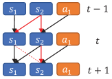
We are interested in tasks where the action and state can be factorized into multiple variables, and formalize such a task as a Factorized MDP (FMDP) denoted by the tuple . Here, , , and respectively denote the state space, action space, and outcome space. Each state is factorized into state variables such that , where is the -th state variable. Similarly, we have for each action and for each outcome. Figure 1(a) illustrates an example of the factorization for a simple 2-grid environment called the Vacuum world Russell et al. (2010). Its state variables include the of the vacuum and whether the places are clean ( and ); it contains only one action variable that is chosen from Left, Right, and Suck (making the place clean). The action of Left or Right leads to an outcome of failure when blocked by the world boundary.
On each step, the agent observes the current state and takes an action , then the state transits and the outcome is produced according to the transition probability , leading to a transition tuple denoted as . Meanwhile, the reward is given by the overall reward function . Following the reward decomposition Juozapaitis et al. (2019), we factorize as the summation of reward variables, given by . is the discount factor for computing returns. is the termination condition deciding whether the episode terminates based on the transition . How reward variables and the termination condition depend on the transition is defined by users according to their demands. In those cases where and contain components unknown to users, we may put these components into the outcome variables. That is, we use an outcome variable to indicate the unknown reward, and define the corresponding reward variable as .
4 The Proposed Framework
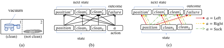
There exist two perspectives on the causal model of the dynamics of the environment: 1) In a unified SCM, action variables are merely nodes of the causal structure and are treated evenly as state variables. 2) In an AIM, each action specifies a peculiar causal structure, leading to a good understanding of both the environment and the agent’s decisions Madumal et al. (2020b). To make it clearer, Figure 1 illustrates how a unified SCM and an AIM pertain to our setting in the above-mentioned Vacuum world. However, directly learning an AIM is intractable as we must divide data into subsets to respectively learn SCMs. This reduces sample efficiency, produces redundant parameters, and cannot be applied to infinite action space. Therefore, we seek to build a unified SCM that can be converted to an AIM based on specially-designed structural equations. As illustrated in Figure 2(a), the exogenous variables in this SCM are the state variables and action variables ; the endogenous variables are the next-state variables and outcome variables . In the following description, we define as the input (exogenous) variables and as the output (endogenous) variables of our model. In this way, a transition tuple can also be written as .
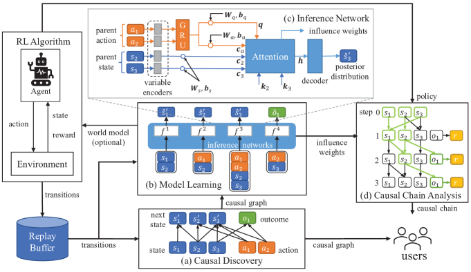
The workflow of the proposed framework is illustrated in Figure 2. When the agent interacts with the environment, we store the transition data into a replay buffer . Using the stored transitions, we perform causal discovery to identify the causal graph of the above-mentioned SCM. Then, we fit the causal equations for the variables of the next state and the outcome using Inference Networks. Together with the known reward function and termination condition , we construct a causal world model that captures the dynamics of the environment. The attention weights (influence weights) in the inference networks capture the action influence, which allows us to perform causal chain analysis to reveal the variables that are causally influenced by the agent’s action. The discovered causal graph interprets the environmental dynamics, and the causal chain analysis provides explanations about the agent’s decisions. Moreover, this causal world model can be used by MBRL algorithms to facilitate learning.
4.1 Causal Discovery
We assume that output variables are produced independently conditioned on the input variables , as independence underlies the intuition of humans to segment the world into components. Under this assumption, it is proven that the causal graph is bipartite, where no lateral edge exists in , and each edge starts in and ends in . Therefore, we only need to determine whether there exists a causal edge for each variable pair , where and . Studies have shown that conditional independent tests (CITs) can be used to perform efficient causal discovery Wang et al. (2022); Ding et al. (2022). In this work, we implement CITs through Fast CIT Chalupka et al. (2018) and determine each edge using the following rule:
| (3) |
where denotes all variables in other than . In Appendix A, we provide the theoretical basics of causal discovery and prove a theorem showing that Equation 3 leads to sound causal graphs.
4.2 Attention-based Inference Networks
To perform causal inference on the discovered causal graph, we fit the structural equation of each output variable using an inference network denoted as , which takes the causal parents as inputs and predicts the posterior distribution . These inference networks should adapt to the structural changes of the causal graph, as the agent’s exploratory behaviors may reveal undiscovered causal relationships and lead to new causal structures. To achieve this, Ding et al. Ding et al. (2022) use Gated Recurrent Unit (GRU) networks that sequentially input all parent variables without discriminating the state and the action. To model the action influence, we design the attention-based inference networks as illustrated in Figure 2(c).
To handle heterogenous input variables (which may be scalars or vectors of different lengths), we first use variable encoders (each uniquely belongs to an input variable) to individually map the input variables to vectors of the same length. These encoders are shared by the inference networks of all output variables. In particular, we use to denote these encoding vectors of input variables.
Then, for each inference network , we compute the contribution vectors of the parent state variables through linear transforms:
| (4) |
The usage of these contribution vectors is equal to the “value vectors” in key-value attention. We use the term “contribution vectors” since the word “value” is ambiguous in the context of RL.
Each inference network contains a GRU network , which receives the action variables in and outputs the action embedding . Then, we feed this action embedding into linear transforms to respectively obtain the query vector and the action contribution vector :
| (5) | |||
| (6) | |||
| (7) |
The projection matrices and bias vectors are all trainable parameters of . We use the superscript to indicate that these parameters belong to .
Each state variable is allocated a key vector , which is a trainable parameter learned by gradient descent. We do not use the superscript for key vectors as they are shared by inference networks of all output variables. The influence weights (i.e., attention weights) of the state variables in and the action are then computed by
| (8) |
| (9) |
We then compute the hidden representation of the posterior distribution using the weighted sum of the value vectors:
| (10) |
Finally, the distribution decoder maps to the predicted posterior distribution:
| (11) |
We assume the type of this posterior distribution is previously known and only outputs the parameters of the distribution. In our implementation, we use normal distribution (parameterized by the mean and variance) for real-number variables and use categorical distribution (parameterized by the probability of each class) for discrete variables.
The inference networks are trained by maximizing the log-likelihood of the transition data stored in , written as
| (12) |
4.3 Causal Chain Analysis
In order to generate explanations, we first describe how our model can be converted to an AIM. Noticing that the key vectors are trainable parameters, the influence weights only depend on the numeric value of action variables. Therefore, the influence weight captures how much the output variable depends on state variable under the given action . In order to generate laconic explanations, we define as the parent set of with salient dependencies under the action , where is a given threshold. In this way, we convert the SCM to an AIM, where the structural equation for under action is written as
| (13) |
Since we use the AIM for the purpose of explanation, it is tolerable to set a larger threshold, which allows us to ignore parent variables that are not influential enough. Madumal et al. have introduced methods to generate good explanations using an AIM. The key is to build a causal chain containing the variables that (i) are causally affected by the actions, and (ii) causally lead to rewards. A single causal chain starting from state and action leads to the explanation for “why the agent took on ”. Contrastive explanations for “why the agent took instead of on ” can be obtained by comparing the causal chines produced by the factual action and the counterfactual action . Details can be found in Appendix B and the AIM paper Madumal et al. (2020a).
The rest of this section introduces how to derive a causal chain starting from the state at step and an action (can be factual or counterfactual) using our model. First of all, we use our model and the agent’s policy to simulate the most-likely trajectory , where denotes the number of simulation steps. The symbol denotes the transition tuple on step , where the actions for are produced by the agent’s policy. For a factual causal chain, this simulation is not necessary if factual data of these future states and actions is available.
Then, we build an extended graph containing the state, outcome, and reward variables of these steps. The edges of this graph accord to the structure of the AIM derived above. That is, if then there exists an edge from to for all . It is worth mentioning that we treat the first transition differently since is exactly the action being explained: If , then is not affected by the choice of . In this case, no edge will be established from any state to .
Afterward, the explainee may specify the target variables (a subset of reward variables) he/she is interested in. Otherwise, all reward variables will be considered. We perform a graph search from the starting state variables and highlight all paths from to the target rewards. These paths together form the causal chain of action starting from . Based on this causal chain, the explanation can be presented as a picture or a natural-language description.
4.4 Model-based RL
XAI literature has widely discussed the trade-off between interpretability and performance, which is also reflected in our model. A sparser causal graph (discovered using a smaller threshold ) is usually easier to read and produces clearer explanations. However, it also enforces the model to infer posterior distributions using less information from input variables , leading to inferior accuracy. In Appendix C, we provide a theorem that formally shows that decreasing the threshold leads to a denser causal graph (i.e., lower interpretability) and also higher predicting accuracy.
In order to show our model is accurate enough to do more than generate post-hoc explanations, we consider applying our world model to MBRL to facilitate policy learning. We use a bootstrap ensemble containing 5 models to alleviate the effect of the epistemic uncertainty Chua et al. (2018). For each iteration, we first collect real transition data into the model buffer . Then, we update the world model by causal discovery and fitting structural equations using the data in . Afterward, we perform -step model-rollouts Janner et al. (2021) to generate simulated data for updating the policy. In our implementation, the policy is trained using Proximal Policy Optimization Schulman et al. (2017). The pseudo-code of the learning procedure is given in Appendix D.
5 Experiments
We present examples of causal chains in two representative environments: Lunarlander-Continuous for the continuous action space, and Build-Maine for the discrete action space. To verify whether our approach can produce correct causal chains, we design an environment to measure the accuracy of recovering causal dependencies of the ground-truth AIM. To evaluate the performance of our model in MBRL, we perform experiments in two extra environments: Cartpole and Lunarlander-Discrete. The Build-Marine environment is adapted from one of the StartCraftII mini-games in SC2LE Samvelyan et al. (2019); the Cartpole and Lunarlander environments are classic control problems provided by OpenAI Gym Brockman et al. (2016). Our source code is available at https://github.com/EaseOnway/Explainable-Causal-Reinforcement-Learning.
5.1 Explanation Results
5.1.1 Lunarlander-Continuous
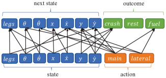
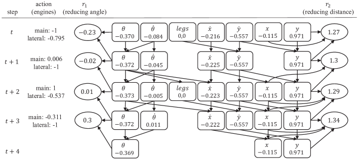
We factorize the state into 7 variables indicating 1) the horizontal position, 2) the vertical position, 3) the horizontal velocity, 4) the vertical velocity, 5) the angle, 6) the angle velocity, and 7) whether the two legs are in contact with the ground. The action includes 2 continuous variables ranged in , respectively controlling the throttles of the main and the lateral engines. The environment contains 3 outcome variables, including 1) the fuel cost due to firing the engine, 2) whether the lander crashed, and 3) whether the rocket is resting.
In this experiment, we learn a post-hoc model to generate explanations for a previously trained policy. We first use the policy (with noise) to collect 150k samples into the buffer . Then, we use these samples to discover the causal graph (with the threshold ) and train the inference networks. The resulting causal graph is presented in Figure 3(a). The environment contains many kinds of rewards, leading to complicated causal chains if we consider them all. To make our explanation clearer, we present a causal chain in Figure 4 considering only two kinds of rewards: 1) the reduction of the distance to the target location, and 2) the reduction of the angle (i.e., balancing the rocket). This causal chain shows that the agent’s action first influences the velocities (, , and ) and thereby reduces (or increases) the angle () and the distance (). In addition, we observe that no parent of the outcome variable is discovered in the causal graph. This means the policy provides insufficient opportunities to reveal its causality. As a result, the variable is excluded from all causal chains, showing that it is not an important consideration in the agent’s policy.
5.1.2 Build-Marine
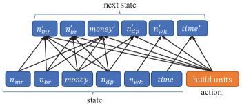
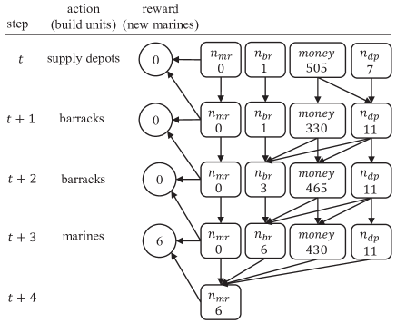
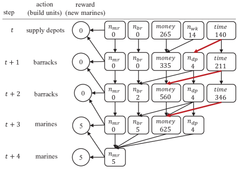
The original observation space provided by the SC2LE interface contains hundreds of variables, which is intractable for causal discovery. In our implementation, we define the state as the tuple containing only 6 variables denoted as , namely 1) the number of workers, 2) the number of marines, 3) the number of barracks, 4) the number of supply depots, 5) the amount of money, and 6) the game time. We are interested in the macro-level decision-making and therefore define the action as one discrete variable indicating which unit (workers, marines, barracks, supply depots, or none) to be built. The micro-level control of building these units (e.g., determining where to place the new barracks) is implemented by simple rules. The goal is to produce as many marines as possible within 15 minutes. Therefore, the player is rewarded with for every newly produced marine. In addition, this environment contains no outcome variable.
In this experiment, both the policy and the causal model are obtained by model-based learning (see Section 4.4). We present the final causal graph in Figure 3(b) (discovered using the threshold ) and an example of the causal chain in Figure 5. The causal chain shows that our attention-based inference networks successfully reason the causal dependencies under different actions, which reflect the following rules of the StarCraftII game: 1) Building new barracks requires at least one supply depot; 2) marines are built from barracks; 3) the number of marines is limited by the number of supply depots; and 4) building more units requires sufficient money in hand. This causal chain explains the reason why the agent builds supply depots: to gain permission to build barracks and provide enough supplies for building marines. Interestingly, we discover no causal relationship between and . For human players, it is common sense that more workers increase the efficiency of collecting minerals and thus lead to a higher income. Since the causal model is learned using the transition data produced along with policy training, this missing edge indicates that the agent explored inadequately for building more workers, providing insufficient evidence to reveal this causal relation.
5.2 Accuracy of Recovering Action Influence
| Direct | Full+Attn | Caus+Attn (ours) | |
| AIM accuracy | 97.0 % | 90.0% | 99.3% |
Good explanations are generated from correct causal chains, which require us to accurately recover the AIMs of environments. In Section 4, we have mentioned a Direct approach that learns the AIM by splitting the data buffer into sub-buffers and performing causal discovery for each action . Though this direct approach is theoretically sound, it suffers from poor sample efficiency and high computational complexity. Noticing that the causal dependencies under different actions usually share similar structures, our approach takes 2 stages: 1) In the causal stage, we learn a unified SCM, whose causal graph summarizes causal dependencies for all actions; 2) in the attention stage, we then transfer this SCM into an AIM based on attention weights (influence weights).
To verify whether our approach can accurately recover the AIM, we design a simple environment that contains spurious correlations to confuse neural networks (see Appendix E.2 for details). We compare our approach with two baselines: 1) the Direct approach mentioned above, and 2) a non-causal approach that uses a full causal graph and only relies on attention. The accuracy of recovering the ground-truth causal dependencies of the AIM using non-i.i.d data is shown in Table 1. These results show that: 1) the causal graph discovered in the causal stage precludes most spurious correlations, making our approach more effective than the Direct approach in practice; 2) and attention alone is insufficient to accurately extract the causal influence of actions.
Further, we examined the causal chains derived solely from attention (where full causal graphs are used). In these chains, we found plenty of spurious correlations, which lead to unreasonable explanations (e.g., “the number of supply depots naturally grows with time” in Build-Marine). An example of such a causal chain and the related discussion are provided in Appendix F. This result shows that causal discovery is an indispensable process for producing reasonable explanations.
5.3 Performance in Model-Based RL
We evaluate the performance of model-based policy learning using our explanatory model. We compare the learning performance with the Model-Free approach that learns policies without models. In addition, we consider two dense models as baselines: 1) the model that concatenates all exogenous variables as inputs and infers endogenous variables using a Multi-Layer Perceptron (MLP), and 2) the Full model that adopts the same networks as ours whereas uses a full causal graph.
The MLP model is the most commonly used in MBRL, and the Full model follows the state-of-the-art modular architecture Ke et al. (2021). These dense models are not suitable for generating explanations. However, they are more accurate (if well-trained) than our explainable model as they are allowed to predict each output variable based on the complete inputs. Existing studies show that causal models generalize better than dense models Wang et al. (2022); Ding et al. (2022). However, we focus on ordinary learning problems and do not consider using our model for generalization. Therefore, we stress that the goal of this experiment is not to obtain a higher performance than dense baselines. On the contrary, We aim to figure out: 1) whether the proposed model can be of help to the learning process, and 2) how much performance our sparse model sacrifices for improved explainability.
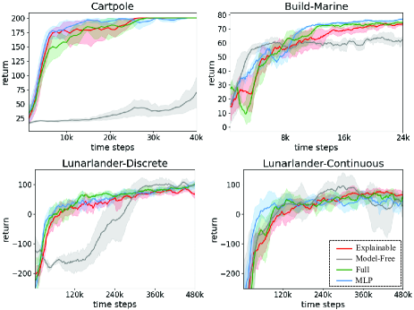
The learning curves are shown in Figure 6. In all environments, the performance of our explanatory model is very close to the dense baselines. Compared to the model-free approach, the model-based approaches significantly learn faster in Cartpole and Lunarlander-Discrete and converge to higher returns in Build-Marine. The returns of all tested approaches are close in Lunarlander-Continuous, whereas the model-based approaches improve the stability of learning. These results show that our model improves explainability at an acceptable cost in performance and well balances the interpretability-accuracy trade-off. Therefore, our model can simultaneously guide policy learning and explain decisions, leading to better consistency between explanations and the agent’s cognition of the environment.
6 Conclusion and Future Work
This paper proposes a framework that learns a causal world model to generate explanations about agents’ actions. To achieve this, we perform causal discovery to identify the causal structure in the environment and fit causal equations through attention-based inference networks. These inference networks produce the influence weights that capture the influence of actions, which allow us to perform causal chain analysis in order to generate explanations. The proposed framework does not require the structural knowledge provided by human experts and is applicable to infinite action spaces. Apart from generating explanations, we successfully applied our model to model-based RL, showing that the model can be the bridge between learning and explainability.
A weakness of our approach is that it requires a known factorization of the environment, which limited its application scope. There exists a number of studies aiming to learn the causal feature set from raw observations Zhang et al. (2020); Volodin (2021); Zhang et al. (2021). Future work will put representation learning into consideration for better applicability. In addition, we currently consider model-based policy learning as the usage of our model apart from generating explanations. However, this usage does not make full use of the advantage of a causal model. Future work will investigate better usage of our model to further improve learning.
Acknowledgments
This work was supported in part by National Key RD Program of China (No.2022ZD0116405) and in part by the National Nature Science Foundation of China under Grant (62073324).
References
- Amir and Amir [2018] Dan Amir and Ofra Amir. HIGHLIGHTS: Summarizing Agent Behavior to People. In Proceedings of the 17th International Conference on Autonomous Agents and Multiagent Systems, Stockholm, Sweden, 2018.
- Atrey et al. [2020] Akanksha Atrey, Kaleigh Clary, and David Jensen. Exploratory Not Explanatory: Counterfactual Analysis of Saliency Maps for Deep Reinforcement Learning, February 2020. arXiv:1912.05743 [cs].
- Bach et al. [2015] Sebastian Bach, Alexander Binder, Grégoire Montavon, Frederick Klauschen, Klaus-Robert Müller, and Wojciech Samek. On Pixel-Wise Explanations for Non-Linear Classifier Decisions by Layer-Wise Relevance Propagation. PLOS ONE, 10(7):e0130140, July 2015.
- Brockman et al. [2016] Greg Brockman, Vicki Cheung, Ludwig Pettersson, Jonas Schneider, John Schulman, Jie Tang, and Wojciech Zaremba. OpenAI Gym, June 2016. arXiv:1606.01540 [cs].
- Chalupka et al. [2018] Krzysztof Chalupka, Pietro Perona, and Frederick Eberhardt. Fast Conditional Independence Test for Vector Variables with Large Sample Sizes, April 2018. arXiv:1804.02747 [cs, stat].
- Chua et al. [2018] Kurtland Chua, Roberto Calandra, Rowan McAllister, and Sergey Levine. Deep Reinforcement Learning in a Handful of Trials using Probabilistic Dynamics Models, November 2018. arXiv:1805.12114 [cs, stat].
- Cohen et al. [2020] Alexandra O. Cohen, Kate Nussenbaum, Hayley M. Dorfman, Samuel J. Gershman, and Catherine A. Hartley. The rational use of causal inference to guide reinforcement learning strengthens with age. npj Science of Learning, 5(1):16, December 2020.
- Coppens et al. [2019] Youri Coppens, Kyriakos Efthymiadis, Tom Lenaerts, and Ann Nowe. Distilling Deep Reinforcement Learning Policies in Soft Decision Trees. In Proceedings of the IJCAI 2019 Workshop on Explainable Artificial Intelligence, pages 1–6, 2019.
- Dietterich et al. [2018] Thomas G. Dietterich, George Trimponias, and Zhitang Chen. Discovering and Removing Exogenous State Variables and Rewards for Reinforcement Learning, June 2018. arXiv:1806.01584 [cs, stat].
- Ding et al. [2022] Wenhao Ding, Haohong Lin, Bo Li, and Ding Zhao. Generalizing Goal-Conditioned Reinforcement Learning with Variational Causal Reasoning, July 2022. arXiv:2207.09081 [cs, stat].
- Fukuchi et al. [2017] Yosuke Fukuchi, Masahiko Osawa, Hiroshi Yamakawa, and Michita Imai. Autonomous Self-Explanation of Behavior for Interactive Reinforcement Learning Agents. In Proceedings of the 5th International Conference on Human Agent Interaction, pages 97–101, Bielefeld Germany, October 2017. ACM.
- Gunning et al. [2019] David Gunning, Mark Stefik, Jaesik Choi, Timothy Miller, Simone Stumpf, and Guangzhong Yang. XAI—Explainable artificial intelligence. SCIENCE ROBOTICS, 4(7120):2, 2019.
- Janner et al. [2021] Michael Janner, Justin Fu, Marvin Zhang, and Sergey Levine. When to Trust Your Model: Model-Based Policy Optimization, November 2021. arXiv:1906.08253 [cs, stat].
- Joo and Kim [2019] Ho-Taek Joo and Kyung-Joong Kim. Visualization of Deep Reinforcement Learning using Grad-CAM: How AI Plays Atari Games? In 2019 IEEE Conference on Games (CoG), pages 1–2, 2019. ISSN: 2325-4289.
- Juozapaitis et al. [2019] Zoe Juozapaitis, Anurag Koul, Alan Fern, Martin Erwig, and Finale Doshi-Velez. Explainable Reinforcement Learning via Reward Decomposition. In Proceedings of the IJCAI 2019 Workshop on Explainable Artificial Intelligence, pages 1–7, 2019.
- Kaiser et al. [2020] Lukasz Kaiser, Mohammad Babaeizadeh, Piotr Milos, Blazej Osinski, Roy H. Campbell, Konrad Czechowski, Dumitru Erhan, Chelsea Finn, Piotr Kozakowski, Sergey Levine, Afroz Mohiuddin, Ryan Sepassi, George Tucker, and Henryk Michalewski. Model-Based Reinforcement Learning for Atari, February 2020. arXiv:1903.00374 [cs, stat].
- Ke et al. [2021] Nan Rosemary Ke, Aniket Didolkar, Sarthak Mittal, Anirudh Goyal, Guillaume Lajoie, Stefan Bauer, Danilo Rezende, Yoshua Bengio, Michael Mozer, and Christopher Pal. Systematic Evaluation of Causal Discovery in Visual Model Based Reinforcement Learning, July 2021. arXiv:2107.00848 [cs, stat].
- Koul et al. [2018] Anurag Koul, Sam Greydanus, and Alan Fern. Learning Finite State Representations of Recurrent Policy Networks, November 2018. arXiv:1811.12530 [cs, stat].
- Longo et al. [2020] Luca Longo, Randy Goebel, Freddy Lecue, Peter Kieseberg, and Andreas Holzinger. Explainable Artificial Intelligence: Concepts, Applications, Research Challenges and Visions. In Machine Learning and Knowledge Extraction, volume 12279, pages 1–16. Springer International Publishing, Cham, 2020. Series Title: Lecture Notes in Computer Science.
- Lu et al. [2018] Chaochao Lu, Bernhard Schölkopf, and José Miguel Hernández-Lobato. Deconfounding Reinforcement Learning in Observational Settings, December 2018. arXiv:1812.10576 [cs, stat].
- Madumal et al. [2020a] Prashan Madumal, Tim Miller, Liz Sonenberg, and Frank Vetere. Distal Explanations for Model-free Explainable Reinforcement Learning, September 2020. arXiv:2001.10284 [cs].
- Madumal et al. [2020b] Prashan Madumal, Tim Miller, Liz Sonenberg, and Frank Vetere. Explainable Reinforcement Learning through a Causal Lens. Proceedings of the AAAI Conference on Artificial Intelligence, 34(03):2493–2500, April 2020.
- Nagabandi et al. [2018] Anusha Nagabandi, Gregory Kahn, Ronald S. Fearing, and Sergey Levine. Neural network dynamics for model-based deep reinforcement learning with model-free fine-tuning. In 2018 IEEE International Conference on Robotics and Automation (ICRA), pages 7559–7566, 2018.
- Nair et al. [2019] Suraj Nair, Yuke Zhu, Silvio Savarese, and Li Fei-Fei. Causal Induction from Visual Observations for Goal Directed Tasks, October 2019. arXiv:1910.01751 [cs, stat].
- Nikulin et al. [2019] Dmitry Nikulin, Anastasia Ianina, Vladimir Aliev, and Sergey Nikolenko. Free-Lunch Saliency via Attention in Atari Agents. In 2019 IEEE/CVF International Conference on Computer Vision Workshop (ICCVW), pages 4240–4249, Seoul, Korea (South), October 2019. IEEE.
- Pearl et al. [2016] Judea Pearl, Madelyn Glymour, and Nicholas P. Jewell. Causal inference in statistics: a primer. Wiley, Chichester, West Sussex, 2016.
- Pearl [2000] Judea Pearl. Causality: models, reasoning, and inference. Cambridge University Press, Cambridge, U.K. ; New York, 2000.
- Peters et al. [2017] Jonas Peters, Dominik Janzing, and Bernhard Schölkopf. Elements of causal inference: foundations and learning algorithms. Adaptive computation and machine learning series. The MIT Press, Cambridge, Massachuestts, 2017.
- Puiutta and Veith [2020] Erika Puiutta and Eric MSP Veith. Explainable Reinforcement Learning: A Survey, May 2020. arXiv:2005.06247 [cs, stat].
- Raffin et al. [2019] Antonin Raffin, Ashley Hill, René Traoré, Timothée Lesort, Natalia Díaz-Rodríguez, and David Filliat. Decoupling feature extraction from policy learning: assessing benefits of state representation learning in goal based robotics, June 2019. arXiv:1901.08651 [cs, stat].
- Russell et al. [2010] Stuart J. Russell, Peter Norvig, and Ernest Davis. Artificial intelligence: a modern approach. Prentice Hall series in artificial intelligence. Prentice Hall, Upper Saddle River, 3rd ed edition, 2010.
- Samvelyan et al. [2019] Mikayel Samvelyan, Tabish Rashid, Christian Schroeder de Witt, Gregory Farquhar, Nantas Nardelli, Tim G. J. Rudner, Chia-Man Hung, Philip H. S. Torr, Jakob Foerster, and Shimon Whiteson. The StarCraft Multi-Agent Challenge, December 2019. arXiv:1902.04043 [cs, stat].
- Schulman et al. [2017] John Schulman, Filip Wolski, Prafulla Dhariwal, Alec Radford, and Oleg Klimov. Proximal Policy Optimization Algorithms, August 2017. arXiv:1707.06347 [cs].
- Seitzer et al. [2021] Maximilian Seitzer, Bernhard Schölkopf, and Georg Martius. Causal Influence Detection for Improving Efficiency in Reinforcement Learning, December 2021. arXiv:2106.03443 [cs].
- Selvaraju et al. [2020] Ramprasaath R. Selvaraju, Michael Cogswell, Abhishek Das, Ramakrishna Vedantam, Devi Parikh, and Dhruv Batra. Grad-CAM: Visual Explanations from Deep Networks via Gradient-based Localization. International Journal of Computer Vision, 128(2):336–359, February 2020. arXiv:1610.02391 [cs].
- Shi et al. [2021] Wenjie Shi, Gao Huang, Shiji Song, Zhuoyuan Wang, Tingyu Lin, and Cheng Wu. Self-Supervised Discovering of Interpretable Features for Reinforcement Learning. IEEE Transactions on Pattern Analysis and Machine Intelligence, pages 1–1, 2021.
- Sloman [2005] Steven Sloman. Causal Models: How People Think about the World and Its Alternatives. Oxford University Press, 08 2005.
- Spirtes et al. [2001] Peter Spirtes, Clark Glymour, and Richard Scheines. Causation, Prediction, and Search. The MIT Press, 2001.
- Volodin [2021] Sergei Volodin. CauseOccam : Learning Interpretable Abstract Representations in Reinforcement Learning Environments via Model Sparsity. PhD thesis, École Polytechnique Fédérale de Lausanne, 2021.
- Wang et al. [2021a] Lingxiao Wang, Zhuoran Yang, and Zhaoran Wang. Provably Efficient Causal Reinforcement Learning with Confounded Observational Data. In Advances in Neural Information Processing Systems, volume 34, pages 21164–21175. Curran Associates, Inc., 2021.
- Wang et al. [2021b] Rui Wang, Xiaoqian Wang, and David I. Inouye. Shapley Explanation Networks, April 2021. arXiv:2104.02297 [cs].
- Wang et al. [2022] Zizhao Wang, Xuesu Xiao, Zifan Xu, Yuke Zhu, and Peter Stone. Causal Dynamics Learning for Task-Independent State Abstraction, June 2022. arXiv:2206.13452 [cs].
- Yang et al. [2022] Chao-Han Huck Yang, I.-Te Danny Hung, Yi Ouyang, and Pin-Yu Chen. Training a Resilient Q-Network against Observational Interference, January 2022. arXiv:2102.09677 [cs, eess] version: 3.
- Yau et al. [2020] Herman Yau, Chris Russell, and Simon Hadfield. What Did You Think Would Happen? Explaining Agent Behaviour through Intended Outcomes. In Proceedings of the 34th Conference on Neural Information Processing Systems, Vancouver, Canada, 2020.
- Zhang et al. [2020] Amy Zhang, Clare Lyle, Shagun Sodhani, Angelos Filos, Marta Kwiatkowska, Joelle Pineau, Yarin Gal, and Doina Precup. Invariant Causal Prediction for Block MDPs. In Proceedings of the 37th International Conference on Machine Learning, pages 11214–11224. PMLR, November 2020. ISSN: 2640-3498.
- Zhang et al. [2021] Amy Zhang, Rowan McAllister, Roberto Calandra, Yarin Gal, and Sergey Levine. Learning Invariant Representations for Reinforcement Learning without Reconstruction, April 2021. arXiv:2006.10742 [cs, stat].
Appendix A Causal Discovery
In this section, we introduce some basics of causal discovery and then prove the soundness of our approach for causal discovery. First of all, we introduce the concept of Markov Compatibility Pearl [2000], which describes whether a directed acyclic graph (DAG) is able to represent the dependencies of a group of random variables.
Definition 1 (Markov Compatibility).
Assume is a group (ordered set) of random variables and is a probability function on . Assume is a DAG whose nodes are these variables, where the parent set of is denoted as . If we have
| (14) |
then we say that and are compatible, or that represents .
The goal of causal discovery is to find some DAG to represent a given probability . Now, we introduce two important concepts for causal discovery: the d-separation and causal faithfulness.
Definition 2 (d-separation).
Assume is a DAG on a set of variables, where , , and are disjoint subsets of variables. We say that and is d-separated by on (denoted as ), if every undirected path from to satisfies:
-
1.
There exists a forward chain , a backward chain , or a fork in such that .
-
2.
For every collision structure in , does not contain or any descendant of .
Theorem 1 (d-separation Criterion).
Assume is a DAG of a set of variables. Assume , , and are disjoint subsets of variables. The following propositions hold:
Definition 3 (Causal Faithfulness).
Assume and are respectively a DAG and a probability function on a set of variables. We say that is faithful to , if
| (16) |
for all disjoint subsets , , and of variables.
Causal faithfulness indicates that all conditional independent relationships are due to the structure of the DAG instead of rare coincidence. In fact, studies have shown that if is compatible with , the chance of to be not faithful to is extremely low Spirtes et al. [2001]. In causal discovery, it is usually assumed that the probability is faithful to the DAG that we are looking for, which makes the structure of recognizable.
We have not distinguished exogenous and endogenous variables above. The exogenous variables are considered the inputs of a system, and thus their causality does not need to be discussed. In other words, our causal graph only describes the causality of endogenous variables, whereas the causality of exogenous variables is ignored. Unless otherwise specified, the letter denotes the set of endogenous variables and the letter denotes the set of endogenous variables in the following discussion. Given a probability function of some variables , the goal of causal discovery now becomes determining only the causal parents of endogenous variables in a DAG that represents .
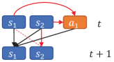
It is worth mentioning that, in the definition given by Pearl Pearl et al. [2016], it is assumed that exogenous variables are independent of each other. However, this requirement is released in our definition since the current state and action variables are usually correlated due to the dependencies underlying the agent’s policy and the history transitions. Ignoring these correlations leads to spurious edges, which are detrimental to generating reasonable explanations. For example, in Figure 7, we show that a backdoor path occurs when the actions are sampled by a policy dependent on the current state; in Figure 7 we show that a backdoor path occurs considering the transition history even if the actions are sampled randomly. In both cases, and are correlated, making an “spurious parent” of in the discovered causal graph.
Therefore, we detect causal dependencies using conditional independent tests (CITs), where the condition variables block all the backdoor paths (if there exist any). We assume that state variables transit and outcome variables arise independently, which brings several benefits: 1) The causal graph is bipartite, making our model able to be computed in parallel. 2) The causal graph can be uniquely identified using CITs. Wang et al. Wang et al. [2022] adopt a similar approach for causal discovery from the perspective of conditional mutual information. Here, we describe and prove a theorem that is used to discover sound causal graphs in our approach.
Theorem 2 (Causal Discovery for Factorized MDP).
Assume and are respectively the sets of exogenous and endogenous variables in a Factorized MDP. Assume that is a probability function of these variables such that is consistent with the MDP; that is, we have
| (17) |
where may follow arbitrary state distribution, can be arbitrary policy, and is the transition probability of the MDP. Then, there always exists a DAG that represents . Further, if we make the following assumptions:
-
1.
(Independent Transition) next-state variables and outcome variables are produced independently, given by
-
2.
(Causal Faithfulness) is faithful to ,
then the following propositions about hold:
-
1.
No lateral edge like exists among . In other worlds, we have for every .
-
2.
The parent sets of are uniquely identified by
for every and every . Here denotes
-
3.
The parent sets of in is invariant. That is, we may replace with any other probability function that satisfies Eq. 17 and obtain a new DAG that represents . Assuming is faithful to , the parent sets of will stays unchanged:
Proof.
We first prove the existence of . Since and in Eq. 17 are both conditional probability function, we write that
where and . Using the chain rule of probability functions, we have
We define
as any subset such that
Similarly, we may define
Together, we will have that
Letting the edges in be given by the parent sets defined above, it is obvious that represents .
Now we assume that the independent transition and causal faithfulness hold.
Assume that contains a lateral edge like for example. According to independent transition, we have . Because , we have . This violates the assumption of causal faithfulness, as we have
Therefore, we prove that no lateral edge among exists in .
Because there is no lateral edge among exists in , blocks all paths form to unless . Therefore, it is easy to prove that
Combining Theorem 1 and Definition 3, we have that
Therefore, the parents of are uniquely identified by the rule:
Finally, let us consider another probability function that satisfies Eq. 17, and assume is the DAG that is compatible with and faithful to. For every it follows that
If and , using the above rule we have and . In other words, we have
This leads to that
We can also write that
From the above equations, we obtain the paradox that
Using reduction to absurdity, we obtain that implies . Similarly, we can prove the opposite direction of this implication. As a result, we have
which shows that .
Proof ends. ∎
Appendix B Explanation through Causal Chains
In our paper, we only present the visualization of causal chains. Although this visualization offers a certain extent of interpretability, Madumal et al Madumal et al. [2020b] have proposed techniques to better use causal chains to generate high-quality explanations. In this section, we introduce how our causal chains adapt to their techniques.
Consider an -step trajectory , where . In this trajectory, we use the bold capital letter to denote the sub-set of variables in the causal chain. In Madumal’s work, an explanation is derived from an “explanan”, which contains information about how action leads to rewards.
Definition 4 (Explanan).
A -step explanan for an action under a factual trajectory is a tuple , where
-
1.
contains the reward variables in the causal chain.
-
2.
is the heading variables (the state variables at the beginning) in the causal chain.
-
3.
contains some intermediate variables between and .
An explanation for “why the agent took action at ” is generated by filling the values in the explanan into a natural-language template. If contains all intermediate variables, the explanan is called a complete explanan. However, it may contain too much information and difficult to be understood. Therefore, Madumal et al suggest using the minimally complete explanan (MCE), where contains only the parents of .
Taking the causal chain in the paper’s Figure 5 for example, we present the explanations respectively drawn from the complete explanan and the minimally complete explanan below.
Example 1 (Complete Explanation for Build-Marine).
The agent build supplies depots because this action causes the following changes:
-
1.
Instantly, the number of supply depots increases from 7 to 11, and money decreases from 505 to 330;
-
2.
After 2 steps, the number of barracks increases from 1 to 3, and the amount of money increases from 330 to 465.
-
3.
After 3 steps, the number of barracks increases from 3 to 6, and the amount of money decreases from 330 to 430.
-
4.
After 4 steps, the number of marines increases from 0 to 6.
Which lead to a reward of due to new marines after 4 steps.
Example 2 (Minimally Complete Explanation for Build-Marine).
The agent builds supplies depots because this action would eventually cause the number of marines to increase from 0 to 6 after 4 steps, which leads to a reward of due to new marines.
In addition, by comparing two MCEs, we can construct contrastive explanations that answer why that agent did not take another action. Therefore, Madumal et al define the minimally complete contrastive explanation, which contains the difference between the factual MCE and the counterfactual MCE.
Definition 5 (Minimally Complete Contrastive Explanation).
Let denote the factual trajectory (the trajectory that actually happens) and denote the counterfactual trajectory, which is produced by replacing with another action and using the world model and policy to simulate the following steps. Assume that is the MCE for under the factual trajectory and that is the MCE for under the counterfactural trajectory. A minimally complete contrastive explanation (MCCE) is then given by a tuple , where
-
1.
is the subset of variables in that 1) is not included in , or 2) owns a value different from that in .
-
2.
is the subset of variables in that 1) is not included in , or 2) owns a value different from that in .
-
3.
contains the reward variables in the factual causal chain.
Appendix C The Trade-off between interpretability and accuracy
Theorem 3.
Assume is an endogenous variable of the SCM of the Factorized MDP. Let and respectively denote its parent sets discovered using the threshold and . Assume is the ground-truth parent set of . If , with the well trained structural equation we have
| (18) | ||||
Proof.
Obviously, we have . For simplicity, we define
where are non-overlapping subsets of . More specifically, are the true parents of , whereas are false parents of . Then we have
We use to denote that a probability conforms to a given distribution. Noted that variables in are not true parents of , with well trained , the posterior distribution of is given by
| (19) |
Therefore, we have
| (20) | ||||
Similarly, we have
| (21) | ||||
Together, we write
| (22) | ||||
∎
Appendix D The Algorithm for Model-Based RL
See Algorithm 1.
Appendix E Environments
E.1 Factorization of Public Environments
This section describes how environments are considered Factorized MDPs in our implementation.
Cartpole
The state is factorized into 4 variables indicating the 1) position of the cart, 2) velocity of the cart, 3) angle of the pole, and 4) angle velocity of the pole. The action only contains one discrete variable indicating the direction (left or right) to push the cart. The goal of the agent is to keep the pole upright as long as possible. Therefore, the agent is rewarded by for each step as long as the state satisfies and . The episode terminates if this condition does not hold. In addition, no outcome variable is included in this environment.
Lunarlander-Discrete The state is factorized into 7 variables indicating the (1) horizontal position, (2) vertical position, (3) horizontal velocity, (4) vertical velocity, (5) angle, (6) angle velocity, and (7) whether the two legs are in contact with the ground. The action contains one discrete variable indicating the engine (none, main, left, or right) to be actuated. The environment contains 3 outcome variables, including (1) the fuel cost due to firing the engine, (2) whether the lander crashed, and (3) whether the rocket is resting. The agent is rewarded (or penalized) from multiple sources, including (1) shortening the distance to the destination, (2) reducing the velocity, (3) reducing the angle, (4) increasing the number of landed legs, (5) being resting, and (6) crashing.
Lunarlander-Continuous replaces the action space of Lunarlander-Discrete with a continuous action space. The new action space includes 2 continuous variables ranged in , respectively controlling the throttles of the main and the lateral engines.
Build Marine The state includes 6 variables denoted as , namely the (1) number of workers, (2) number of marines, (3) number of barracks, (4) number of supply depots, (5) amount of money, and (6) game time. The action includes only one discrete variable indicating which unit (workers, marines, barracks, supply depots, or none) to be built. The player is rewarded with for every newly produced marine. The problem is challenging since marines can only be built from barracks, and barracks can only be built provided there exists at least one supply depot. In addition, the number of workers and marines is limited by the number of supplies provided by supply depots.
E.2 The Environment for Measuring the Accuracy of Recovering Action Influence
To measure the accuracy of recovering the causal dependencies of the AIM, we design an additional environment with a known ground-truth AIM. The environment contains one action variable and 5 state variables: and . The action variable is chosen from 4 options . The dynamics of these state variables are given by
| (23) | ||||
| (26) | ||||
| (31) | ||||
| (32) | ||||
| (37) |
The ground-truth causality of the AIM can be easily derived from the above dynamics. Aiming to confuse neural networks, these dynamics create copious spurious correlations in the data. For example, and present a strong positive correlation, whereas neither of them is the other’s causation.
Appendix F Importance of Causality: an Example
To show how causal discovery facilitates explanation generation, we investigated the causal chains produced without a discovered causal graph. Figure 8 presents such a causal chain for Build-Marine. It is produced by our model using a full graph, where unreasonable connections are highlighted in bold and red. We found the model attributes a large influence weight () to as the salient parent of under the action of building supply depots. This leads to the incorrect understanding that “if we build supply depots, the number of supply depots turns to because the game time is ”. In fact, the variable only influences in the discovered causal graph presented in Figure 3(b), meaning the number of supply depots is not caused by the game time at all. The model is misled by the fact that the agent always builds more supply depots as time goes on, which makes the two variables ( and ) highly related. Similarly, the model wrongly takes as the salient parent of under the actions of building barracks since it observes that money usually accrues with time.
Therefore, attention alone is insufficient to obtain reasonable causal chains for explanations, as it can be easily misled by spurious correlations (which are rife in the non-i.i.d. data collected in RL). Fortunately, these errors in causal chains are greatly reduced when combining attention with a causal graph, which precludes most spurious correlations and leads to correct causal chains.
Appendix G Hyper-parameters of Model-based RL
| Parameter | Cartpole | LunarLander | LunarLander-Continuous | Build-Marine |
| total epochs () | 50 | 200 | 200 | 200 |
| environment steps per epoch | 800 | 2400 | 2400 | 120 |
| policy-update rounds per epoch () | 20 | 20 | 20 | 20 |
| epochs per graph update () | ||||
| rollout length | ||||
| rollout samples for policy update | 4096 | 4096 | 4096 | 2048 |
| causal threshold () | 0.1 | 0.3 | 0.4 | 0.15 |
| model-ensemble size | 5 | 5 | 5 | 5 |
| discount factor () | 0.98 | 0.975 | 0.975 | 0.97 |
The main hyper-parameters used in the mentioned environments for model-based RL are presented in Table 2.
Appendix H Computational Complexity
Let roughly denote the number of variables of the environment. Let denote the total number of transition samples. Let denote the batch size.
Model
The parameter scale of our model is . The time complexity of one forward pass is .
Causal discovery
The time complexity of testing each edge through FCIT is and the overall time complexity of causal discovery is . The space complexity for causal discovery is if the tests are sequentially performed.
Causal chains
The time complexity and space complexity of generating an -step causal chain are both . In our experiments, the generation of each causal chain completes almost instantly.