Testing for no effect in regression problems: a permutation approach

Abstract

Often the question arises whether $Y$ can be predicted based on $X$ using a certain model. Especially for highly flexible models such as neural networks one may ask whether a seemingly good prediction is actually better than fitting pure noise or whether it has to be attributed to the flexibility of the model. This paper proposes a rigorous permutation test to assess whether the prediction is better than the prediction of pure noise. The test avoids any sample splitting and is based instead on generating new pairings of $(X_{i},Y_{j})$. It introduces a new formulation of the null hypothesis and rigorous justification for the test, which distinguishes it from previous literature. The theoretical findings are applied both to simulated data and to sensor data of tennis serves in an experimental context. The simulation study underscores how the available information affects the test. It shows that the less informative the predictors, the lower the probability of rejecting the null hypothesis of fitting pure noise and emphasizes that detecting weaker dependence between variables requires a sufficient sample size.

1 Introduction

With the ubiquity of data often the question whether a response $Y$ can be predicted based on predictors $X$ arises. The rise of highly capable machine learning and deep learning techniques increases the abilities to fit any kind of data. However, the abilities to fit pure noise are increasing as well. We propose a method to test whether a model is only fitting noise. It extends testing for no effect from linear to nonlinear models. No sample splitting is performed so the power of the test can rely on the size of the whole sample. No nested sequence of models is needed, in fact, no alternative models are needed at all.

Our method is based on recombining the pairings between predictors and responses through permutations. In this way artificial reference datasets are created and the performance of the model on the original data can then be assessed by comparing it to the performances on the artificial reference datasets. The purpose of our test is to ascertain whether the model is capable of fitting the data more effectively than mere random noise. Our method is not restricted to linear models since it is not a test for specific parameters in the model. Rather it tests for the ability of a model to predict the responses.

The main contribution of this paper is a rigorous formulation of a permutation test for dependence between model predictions and responses. The test uses $R^{2}$ as test statistic but can be performed with any measure of goodness of fit in regression analysis. Because of its interpretability, $R^{2}$ is our test statistic of choice, but this can be adapted if necessary. The method generates new pairings of $(X_{i},Y_{j})$ conditional on the $X_{i}$ for $i=1,...,n$ and $Y_{j}$ for $j=1,...,n$. This paper introduces a new formulation of the null hypothesis and provides a rigorous justification for a permutation test that has been described in various forms in the literature, for instance in the two-sample problem [15, 10, 18, 19], the stochastic dominance problem [2, 3] or the subgroup discovery problem [12]. The main use case for this method is in the initial stages of the data analysis to test whether a given model does only fit noise or is able to capture some essential structure in the data.

The outline of the paper is as follows. Section 2.1 formulates the problem and introduces necessary notation. Section 2.2 provides the historical context and an overview of the current state of the literature on permutation tests in regression problems. Section 2.3 contains the formal formulation of the null hypothesis, theoretical considerations and the succinct description of the method. Section 3.1 presents a simulation study, where the permutation test is demonstrated in various scenarios for predictors and responses. Section 3.2 contains the application of the permutation test to sensor data of tennis serves in order to demonstrate the method in practice and showcase its power in a real-life scenario.

2 Methodology

2.1 Problem description

Consider a regression setting. Given an observed pair $(X,Y)$, where $X$ is a random vector and $Y$ is a real random variable. $Y$ is modelled as:

$$Y=f(X)+\epsilon,$$

where $\epsilon$ is an error term and $f\in\mathcal{F}$ for some class of functions $\mathcal{F}$. An example of $\mathcal{F}$ could be a set of all linear functions corresponding to a linear regression model with fixed number of variables or a set of functions that can be described by a neural network. Nonparametric classes of functions can also be considered, for instance a set of log-concave functions. For the remainder of the paper, we will focus on $R^{2}$ as goodness-of-fit measure.

Since the actual relationship between $X$ and $Y$ is not known in practice, a chosen model $\mathcal{F}$ through which that relationship is described does not need to be appropriate. The class of functions $\mathcal{F}$ is misspecified if it does not contain the true $f$, while if it contains too many functions, the model might be overfitting by memorizing the noise $\epsilon$. In a real world scenario, we are often facing datasets that feature high-dimensional, time-dependent or functional variables. The question whether there is a relationship between $X$ and $Y$ and which model to choose for describing it, is crucial. In this paper, we focus on the following aspect:

• can a given model $\mathcal{F}$ distinguish $Y$ from pure noise?

Consider this simple example. Let $X_{1},X_{2}$ be independent standard normal variables and $Y=X_{1}^{2}+X_{2}^{2}+\epsilon$, where $\epsilon\sim\mathcal{N}(0,0.01)$. Consider a multi-layered neural net as a model of choice to predict $Y$ using $X_{1}$ and $X_{2}$. For small sample sizes shuffling the vector of responses and applying our prediction model to this shuffled dataset can yield values of $R^{2}$ higher than values of $R^{2}$ calculated for the prediction model applied to the original dataset. Ten random samples of size 10 were drawn. Five yielded higher values of $R^{2}$ for at least one shuffled dataset than for the original pairing (we considered 200 shuffles of the sample). In applied settings, where the sample size is fixed and difficult to increase, this presents an inherent issue. Sample size has an immediate influence on the credibility of the model and needs to be taken into account.

Related problems have been addressed before in the literature in different settings and with a variety of solutions. In this paper we focus on the permutation test. To provide context to our solution, we will give a brief review of the existing literature on permutation tests, before we specify the precise null hypothesis.

2.2 Permutation tests in the existing literature

Historically, the idea of permutation tests existed before it was feasible to realize them on a larger scale and one of the main pioneers in that regard was Ronald Fisher. Fisher’s interest in randomization as a concept can be traced back to his 1925 Statistical Methods for Research Workers [14]. His initial idea related to the experimental design and to getting rid of researcher’s bias in the setup of experiments [17]. At that time the use of randomization concerned only experiments with small numbers of samples (as it would be near impossible to apply it in case of large sample sizes). The application of randomization to hypothesis testing first emerged in the 1930s as introduced by Ronald Fisher in the form of a permutation test as the test for comparing the distributions of two independent groups. The use of this test, commonly known as the Fisher-Pitman permutation test, has since been extended to many other settings [6].

The rise of automated computing made these types of tests feasible to use on a larger scale. Since the 1970s, permutation tests have started to enjoy larger popularity. A good example of the renewed interest in permutation tests can be found in [24], which gives a justification based on the principle of unbiasedness for permutation tests. It also gives good reasons for the transition from the $t$-test to a permutation test. The paper [7] discusses the growing popularity of the permutation test as a substitute for the ANOVA F-test and investigates its robustness. Tests of partial regression coefficients in a linear model are considered in [1]. This paper explains the exact test and then compares the distributions of the test statistics under the various permutation methods proposed. The authors use the classic null hypothesis when testing for no effect. An excellent survey of various papers in the biomedical field can be found in [23]. It showcases the appeal of both the randomization in experimental design (as opposed to random sampling) as well as the permutation tests for differences in location. The increased popularity of permutation tests can be seen in other fields as well, e.g. in psychological research [6].

The applications of permutation tests have expanded beyond the comparison of statistical models to a variety of problems. However, the formal formulation of the null hypothesis can be challenging and subject to variations among authors, particularly when permutation tests are utilized as a problem-solving approach. A subset of publications uses the concept of exchangeability, i.e. the joint distribution of the observations is invariant under permutations of the order of the predictors in their formulation of the null hypothesis in the permutation test. Most commonly the null hypothesis is expressed in terms of exchangeability in two-sample problems, e.g. [15, 10, 18, 19]. There have also been studies with regards to the robustness of permutation tests with respect to the assumption of exchangeability, i.e. in cases where exchangeability cannot be assured, what can be said about asymptotic properties of the test. These ideas are explored well, e.g. in [28] and [29]. More recently, a permutation test without the assumption of exchangeability has been applied to the two-sample problem [35]. The null hypothesis is the equality of two population means. Their split sample permutation t-tests are asymptotically exact and can be extended to testing hypothesis about one population.

When discussing permutation tests, the question arises whether a model applies. Many permutation tests are specifically designed to tackle problems within linear regression models. However, there are applications to other models as well. A permutation test for no effect in a functional linear regression model has been proposed in [9]. In this case the randomization technique allows for the simulation of the conditional distribution of the test statistic, which otherwise would be difficult to obtain. Wide attention has been given to the the permutation approach in the stochastic dominance problem in testing for ordered categorical variables, introduced in [2]. Further developments can be found, for instance in [3]. In the problem of testing heterogeneity in two-sample categorical variables, [4] proposes a permutation test. Here, the null hypothesis considered is simply the equality of heterogeneity of two population distributions. In a subgroup discovery problem, [12] employs a randomization technique. The test devised for this purpose is based on a null hypothesis that the quality measure (for instance $R^{2}$) of a given subgroup is generated by the distribution of false discoveries (DFD), which arises from the central limit theorem applied to a set of quality measure values on some baseline subsets. Permutation tests have also been applied to linear mixed models, more specifically as a test for random effects. For instance, [22] presents two permutation tests, one based on the best linear unbiased predictors and another based on the restricted likelihood ratio test statistics. Both methods involve weighted residuals, with the weights determined by the among- and within-subject variance components. The lack of flexibility in permutation tests, particularly in the context of experimental design of the model, is considered by [33, 34]. Their main focus is on the tests of no effect in a general linear model and their main achievement is the unification of a diverse set of results. The outcome is a single permutation strategy with a single generalized measure. It is worth noting that, once again, the assumption of exchangeability is considered in the formulation of the null hypothesis for the permutation test. Permutation approaches have also been applied to nonparametric ANOVA designs as seen in [16]. There the synchronized permutation method is extended specifically to unbalanced two-level ANOVA. The problem of testing independence given a sample from a bivariate distribution has been considered in [11]. The method used there relies on studentizing the sample correlation which leads to a permutation test that is exact under independence while asymptotically controls the probability of type 1 errors. Permutation tests have also been used in an application of a multivariate regression analysis to a study of factors influencing mental health during the COVID-19 lockdown period [8]. In this particular study, a combined permutation test on data collected in a survey is applied. The null hypothesis is that the regression coefficients are zero. An application to weighted regression models can be found in [30]. A comparison of $X$-permutation and $Y$-permutation and their variability in the weights is given there, inspired by the nature of the weighted regression models in which the permutation of the response variables and the permutation of the predictors do not lead to the same result. An extensive overview of permutation tests, their theoretical properties as well as a vast number of applications, can be found in [25].

Overall, the main appeal of permutation tests stems from the fact that they do not require any distributional assumptions on the population. The lack of assumptions is increasingly more interesting to researchers as deep learning methods become more popular since they likewise do not rely on distributional assumptions. Permutation tests are completely data-driven as pointed out by [6]. This can be very appealing as the data is the main factor in shaping the distribution of the test statistic, i.e. the test statistic can be chosen to be more easily interpretable without focusing on its distribution.

Our work differs from previous work most in the formulation of the null hypothesis. Based on the publications mentioned in this section, we have seen a few different null hypotheses. Some involve the concept of exchangeability, some equality of means or zeroing of the coefficients. In contrast to this, we focus on the concept of independence, which is not widely used for permutation tests. Permutation tests of independence have existed before, e.g. [5]. However, we do not test independence of two random variables $X$ and $Y$, but rather we state the null hypothesis in terms of the model and whether it is able to capture the dependence.

The choice of the null hypothesis can also be directly connected to the model considered in the problem. For instance, it is natural to use zeroing of the functional coefficient as the null hypothesis when considering a functional linear regression model [9]. We do not restrict ourselves to any particular model in our work, we only consider the model as given and the null hypothesis is not specifically tailored to the model.

The subsequent section will concentrate on establishing a rigorous theoretical foundation for our permutation test.

2.3 Permutation approach to testing for no effect

Our goal is to investigate whether a model $\mathcal{F}$ can capture any dependence between $X$ and $Y$. We consider a test with null hypothesis stated as follows:

$$H_{0}:Y\textrm{ is independent of }f(X)\textrm{ for all }f\textrm{ in the model }\mathcal{F}.$$ (1)

$H_{0}$ represents the problem as described in section 2.1. If it were true, then our model $\mathcal{F}$ will not be able to capture the relation between $X$ and $Y$ in a meaningful manner. Considering a dataset with permuted responses will be no different to model $\mathcal{F}$ under $H_{0}$. If $H_{0}$ is false, then the model $\mathcal{F}$ will be able to capture some aspects of the relation between $X$ and $Y$, although it does not guarantee that the model is suitable and readily applicable.

The null hypothesis $H_{0}$ as stated in (1) does not guide the choice of the test statistic. In order to choose a suitable test statistic, further understanding of $H_{0}$ is needed.

Proposition 2.1.

Let $(X_{1},Y_{1}),...,(X_{n},Y_{n})$ be an i.i.d. sample of $(X,Y)$. If $f(X)$ and $Y$ are independent for all $f\in\mathcal{F}$, then the conditional distribution of

$$\{(f(X_{i}),Y_{\tau(i)}):f\in\mathcal{F}\}$$ (2)

given the empirical measure $P_{n}^{X}$ of $X_{1},...,X_{n}$ and the empirical measure $P_{n}^{Y}$ of $Y_{1},...,Y_{n}$ is the same for all permutations $\tau$ of set $\{1,...,n\}$.

Proof.

For a given finite collection of functions $f_{1},f_{2},...,f_{m}\in\mathcal{F}$ and a permutation $\tau$, the conditional joint distribution of $(f_{1}(X_{i}),Y_{\tau(i)}),...,(f_{m}(X_{i}),Y_{\tau(i)})$ given $P_{n}^{X}$ and $P_{n}^{Y}$ is the same as the joint distribution of

$$(f_{1}(X_{i}),Y_{i}),...,(f_{m}(X_{i}),Y_{i}),$$ (3)

thanks to the assumption of independence of $f(X)$ and $Y$ for any $f\in\mathcal{F}$. Note that (3) is invariant with respect to the permutations of $Y_{i}$. This statement will also be true if extended to a joint distribution of (2) thanks to Kolmogorov extension theorem [21], hence the distribution of joint conditional distribution of (2) given $P_{n}^{X}$ and $P_{n}^{Y}$ is invariant with respect to the permutation of $Y_{i}$. ∎

Before proposition 2.1 is translated into a result in terms of $R^{2}$, we formally define $R^{2}$. Consider $n$ realizations of $(X,Y)$ and denote them as $(x_{1},y_{1}),...,(x_{n},y_{n})$. Let $L$ be a loss function and $\hat{f}$ be an empirical risk estimator in the sense that

$$\hat{f}=\operatorname*{arg\,min}_{f\in\mathcal{F}}\sum_{i=1}^{n}L(f(X_{i}),Y_{i}).$$ (4)

Let $\hat{f}(x_{i})$ denote the prediction of $y_{i}$ for $i=1,...,n$. Then

$$R^{2}=1-\frac{\sum_{i}(y_{i}-\hat{f}(x_{i}))^{2}}{\sum_{i}(y_{i}-\bar{y})^{2}},$$ (5)

where $\bar{y}$ is the mean of the $y_{i}$. This definition of $R^{2}$ is the natural one if the loss function $L$ in equation (4) is chosen to be the squared error loss. In the context of $R^{2}$, proposition 2.1 implies the following result.

Proposition 2.2.

Let $(X_{1},Y_{1}),...,(X_{n},Y_{n})$ be an i.i.d. sample of $(X,Y)$. Assume that $f(X)$ and $Y$ are independent for all $f\in\mathcal{F}$. Fix a permutation $\tau$ of $\{1,...,n\}$ and a loss function $L$ defining an empirical risk estimator as in (4). Then, conditionally on the empirical measure $P_{n}^{X}$ of $X_{1},...,X_{n}$ and the empirical measure $P_{n}^{Y}$ of $Y_{1},...,Y_{n}$, the distribution of $R^{2}$ calculated based on data $\{(X_{i},Y_{\tau(i)})\}$ using the aforementioned emprirical risk estimator does not depend on $\tau$.

Proof.

Proposition 2.1 implies that the conditional distribution of

$$\Bigg{\{}\left(\sum\limits_{i=1}^{n}(Y_{\tau(i)}-f(X_{i}))^{2},\sum\limits_{i=1}^{n}L(f(X_{i}),Y_{\tau(i)})\right):f\in\mathcal{F}\Bigg{\}}$$ (6)

given $P_{n}^{X}$ and $P_{n}^{Y}$ is the same for all permutations $\tau$ of set $\{1,...,n\}$. This is a two-dimensional empirical process indexed by model $\mathcal{F}$. Plugging in the $\operatorname*{arg\,min}$ of the second component into the first component still gives a distribution that does not depend on $\tau$. Hence, combining the definition (4) of $\hat{f}$ and (5) of $R^{2}$, we conclude that for each permutation $\tau$, $R^{2}$ calculated for $\{(X_{i},Y_{\tau(i)})\}$ is sampled from the same distribution conditioned on $P_{n}^{X}$ and $P_{n}^{Y}$. ∎

This allows us to consider $R^{2}$ as a viable choice for the test statistic. Under the null hypothesis, the $R^{2}$ as calculated for $(x_{i},y_{i})$ is sampled from the same distribution as the $R^{2}$ calculated for $(x_{i},y_{\tau(i)})$ for some permutation $\tau$. The test itself is based on permutations of the pairings $(x_{i},y_{i})$. We reject $H_{0}$ only if the observed $R^{2}$ is much larger than ”most” of the $R^{2}$ obtained via random permutations. Essentially we compare the observed $R^{2}$ to the distribution of $R^{2}$ under $H_{0}$ given specific realizations of $X$ and $Y$, but not their pairings. It is notable that $R^{2}$ can also be replaced by some other statistic, as long as it can be calculated using the sample $\{(f(x_{i}),y_{i})\}_{i}$. Proposition 2.1 permits other statistics to be used instead of $R^{2}$. Taking $R^{2}$ as the test statistic is equivalent to taking empirical risk with respect to quadratic loss as the test statistic. In that sense, the other tests can also be constructed by considering empirical risks with respect to other losses, e.g. absolute loss or Huber loss.

If the model $\mathcal{F}$ contains the constant functions and the predictors are optimized with respect to the quadratic loss, then $R^{2}$ calculated for a given $\mathcal{F}$ is always non-negative. This is true, since given set of observations $\{y_{i}\}_{i=1,...,N}$, we can always choose $f(X)\equiv\frac{1}{N}\sum\limits_{i=1}^{N}y_{i}$ which yields $R^{2}=0$. Note that including the constants in $\mathcal{F}$, does not disturb the independence of $Y$ and $f(X)$ for all $f\in\mathcal{F}$, since $Y$ is always independent of a set of constant random variables. While $R^{2}$ is always non-negative in linear regression models (if the intercept is included), that is not the case for instance in the setting of neural nets.

Given a chosen $\alpha$ level, the precise implementation of the test is as follows:

1. given original pairings of $(x_{i},y_{i})$, calculate the $R^{2}$ of model $\mathcal{F}$, which we will denote as $r_{0}^{2}$,

2. find the distribution of $R^{2}$ under the null hypothesis conditionally on observed $x_{i}$ and $y_{(i)}$ for $i=1,...,n$ (approximated by the empirical distribution function of $R^{2}$ values based on a uniform sample of permutations of original pairings $(x_{i},y_{i})$; for each sample $\{(x_{i},y_{\tau(i)}):1\leq i\leq n\}$, where $\tau$ is a permutation, $R^{2}$ is calculated; notably, the model is refit for each permuted sample),

3. if $r_{0}^{2}>q_{1-\alpha}$, where $q_{1-\alpha}$ is the $1-\alpha$ quantile of the empirical distribution of $R^{2}$ values, then we reject the null hypothesis, otherwise we do not reject it.

Any tuning parameters used in point (1) and (2) are not adjusted for each permutation. This implementation assumes that $R^{2}$ is the statistic of choice, but it can be adapted to suit other statistics as well. The reason we prioritize $R^{2}$ is primarily because of its benefits in terms of interpretability and ease of use. It is also important to note that in practice, determining the distribution of $R^{2}$ under the null hypothesis will not be exact in most cases. To obtain the exact distribution we need to run through $n!$ permutations. Even for $n>10$ the computational cost of such an operation is prohibitively expensive and sampling from the true distribution is more reasonable.

$R^{2}$ is bounded by 1 from above for any model. The proximity of $R^{2}$ values calculated from the permuted data or original $R^{2}$ values to 1 or to each other can provide insight into goodness of fit of a model. The closer the values of $R^{2}$ for the permuted data to 1, the greater the capability of the model to fit to the noise. Close proximity of $q_{1-\alpha}$ to $r_{0}^{2}$ in case of $r_{0}^{2}>q_{1-\alpha}$ and $r_{0}^{2}$ small implies that the model’s predictive ability may not be satisfactory even though the null hypothesis is rejected by the test. The test is widely applicable, because of its general form and easily adaptable to different types of models. It also provides an interesting commentary on the predictive abilities of a chosen model. In the event that the quantile $q_{1-\alpha}$ for one model, $\mathcal{F}_{1}$, significantly exceeds the same quantile for another model, $\mathcal{F}_{2}$, we conclude that $\mathcal{F}_{1}$ is either overfitting, indicating a need for reduction of the set of independent variables or model simplification, or is better able to extract meaningful information from unrelated data.

3 Application

3.1 Simulation study

We apply our permutation test in multiple scenarios. This section will specifically focus on simulated datasets to assess the test’s performance on datasets with varying dependence levels between $X$ and $Y$ and two different models $\mathcal{F}$. An empirical example will be considered in section 3.2. In all scenarios we consider the $R^{2}$-based test.

Two different models will be used to fit the data throughout this section. One of them is a linear regression model, which models the relationship between a random vector $X$ and a random variable $Y$ in a linear manner: $Y=\beta\cdot X+\epsilon$. The parameter vector $\beta$ will always be estimated using the least squares method. Regardless of the length of vector $X$, this model will be referred to as $\mathcal{F}_{\textrm{LR}}$. The other model we consider is a neural net. A neural net is a collection of neurons arranged into layers, with neurons from different layers connected to each other. Typically, a neural net consists of an input layer, multiple hidden layers and an output layer. The estimation of neural nets’ parameters, the weights associated with neurons and edges between them, is done by feeding multiple training sets of inputs and outputs into the net. Weights are adjusted each time based on a predefined cost function. Neural nets will be referred to as $\mathcal{F}_{\textrm{NN}}$ with the number of neurons on each layer specified as a $k$-tuple, where $k$ refers to the number of layers, e.g. $\mathcal{F}_{\textrm{NN}}(30,30,30)$ is a neural net with 3 hidden layers, each of which contains 30 neurons.

Let $X_{1},X_{2}\sim\mathcal{N}(0,1)$ and $Y\sim U([0,1])$ be independent random variables. We consider two models: $\mathcal{F}_{\textrm{LR}}$ and $\mathcal{F}_{\textrm{NN}}(30,30,30)$ and a sample of size $100$. In both cases the null hypothesis is not rejected, see fig. 1(a) and 2(a). We also consider 1000 repetitions of the experiment in the same setup to see the behavior of the test on a larger number of examples. As seen in fig. 1(b) and 2(b), the null hypothesis is rejected in most repetitions for both models, namely 4.7% for the linear model and 4.5% for the neural net. This shows that the rejection of the null hypothesis can still happen even in case of independence. Most importantly, the rejection rate is close to the confidence level $\alpha=5\%$.

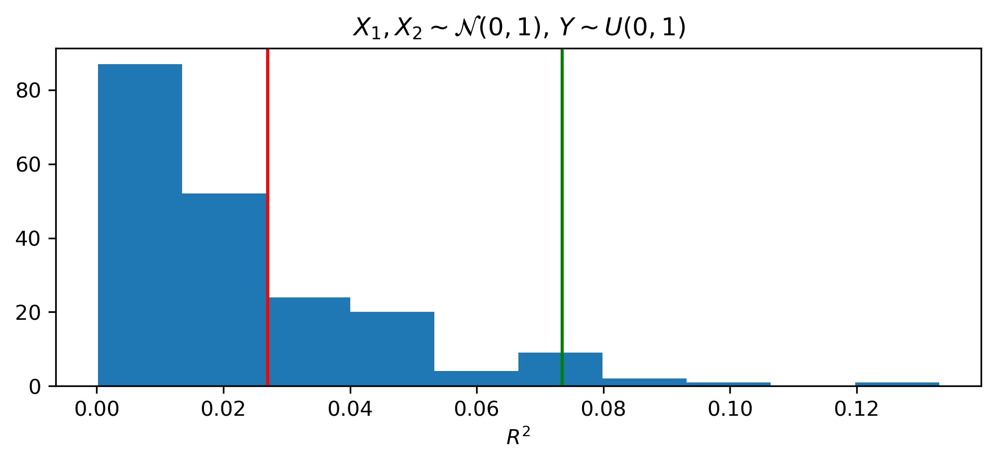
(a) Histogram of the distribution of generated $R^{2}$ using permutation of $y$ values. The model considered here is linear regression $\mathcal{F}_{\textrm{LR}}$. The sample size is 100. The red line denotes the observed $R^{2}$ for the true pairings of $X$ and $Y$, the green line denotes the 95%-quantile of the empirical distribution of $R^{2}$ (approximation using 200 permutations).

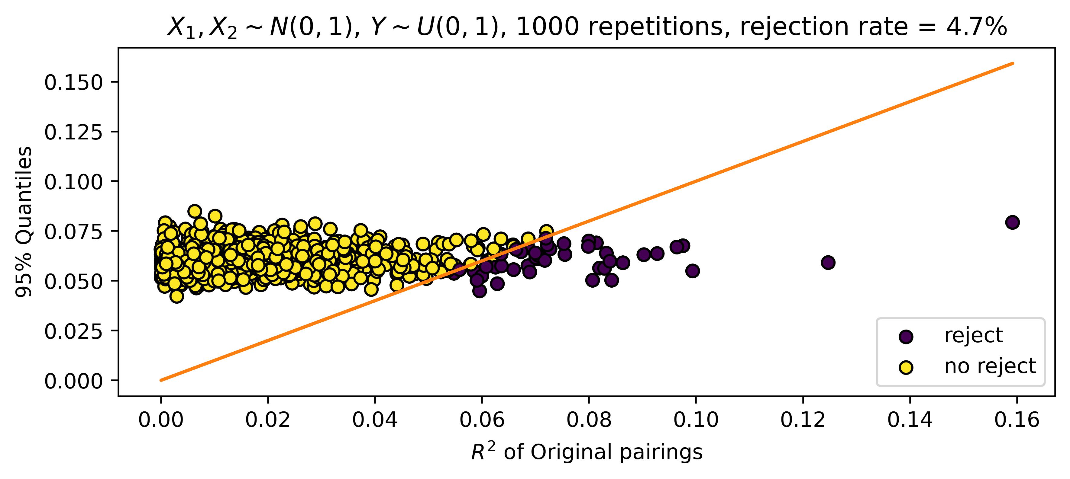
(b) Scatterplot of the $R^{2}$ values for the original pairings against the 95% quantiles of the empirical distribution of $R^{2}$. The orange line shows the identity function.

Figure 1: Results of the permutation test for $\mathcal{F}_{\textrm{LR}}$ with data generated in a following manner $X_{1},X_{2}\sim\mathcal{N}(0,1)$ and $Y\sim U([0,1])$.

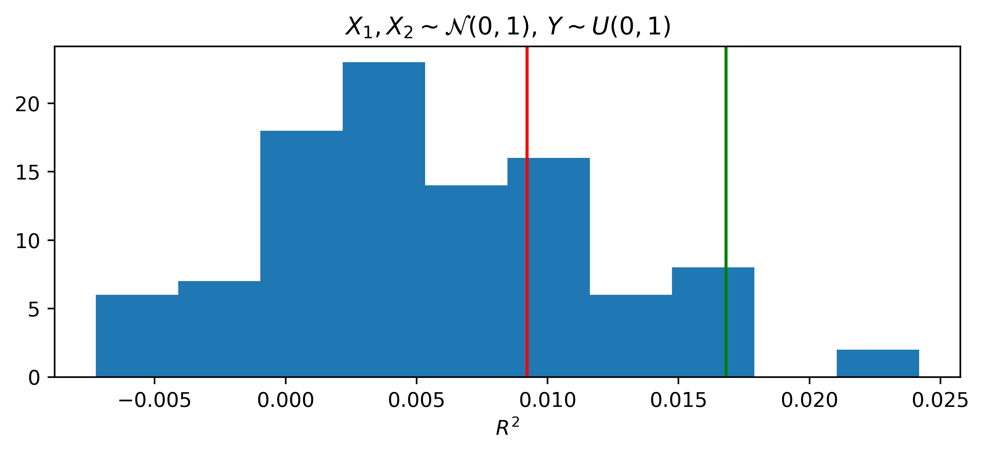
(a) Histogram of the distribution of generated $R^{2}$ using permutation of $y$ values. The model considered here is a 3-layered neural net $\mathcal{F}_{\textrm{NN}}(30,30,30)$. The sample size is 100. The red line denotes the observed $R^{2}$ for the true pairings of $X$ and $Y$, the green line denotes the 95%-quantile of the empirical distribution of $R^{2}$ (approximation using 200 permutations).

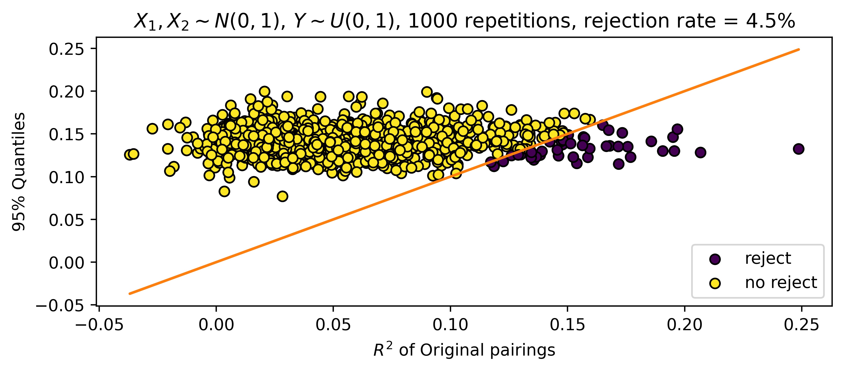
(b) Scatterplot of the $R^{2}$ values for the original pairings against the 95% quantiles of the empirical distribution of $R^{2}$. The orange line shows the identity function.

Figure 2: Results of the permutation test for $\mathcal{F}_{\textrm{NN}(30,30,30)}$ with data generated in a following manner $X_{1},X_{2}\sim\mathcal{N}(0,1)$ and $Y\sim U([0,1])$.

Now, let $X_{1}\sim\mathcal{N}(1,1),X_{2}\sim\mathcal{N}(0,1)$ be independent and $Y=\log|X_{1}|+X_{2}^{2}+\epsilon$, where $\epsilon\sim\mathcal{N}(0,1)$ is the noise. Consider a sample of size $100$. For both $\mathcal{F}_{\textrm{LR}}$ and $\mathcal{F}_{\textrm{NN}}(30,30,30)$, the permutation test rejects the null hypothesis, since the values of $R^{2}$ for the original pairings are much higher than for any of the permuted pairings. For the behavior of the test in a single example see fig. 3(a) and 4(a). In this case the neural net outperforms the linear model significantly, thanks to its complexity. Fig. 3(b) and 4(b) show that the rejection rate in this case is quite high when repeating the experiment 1000 times, close to 95% for the linear model and 94% for the neural net. This particular example illustrates the test’s applicability in the case of a functional relation between predictors and responses. The model is not just fitting the noise, there is some relation between predictors and responses. It might not be captured well using a linear regression model, but the model is still able to capture more than pure noise.

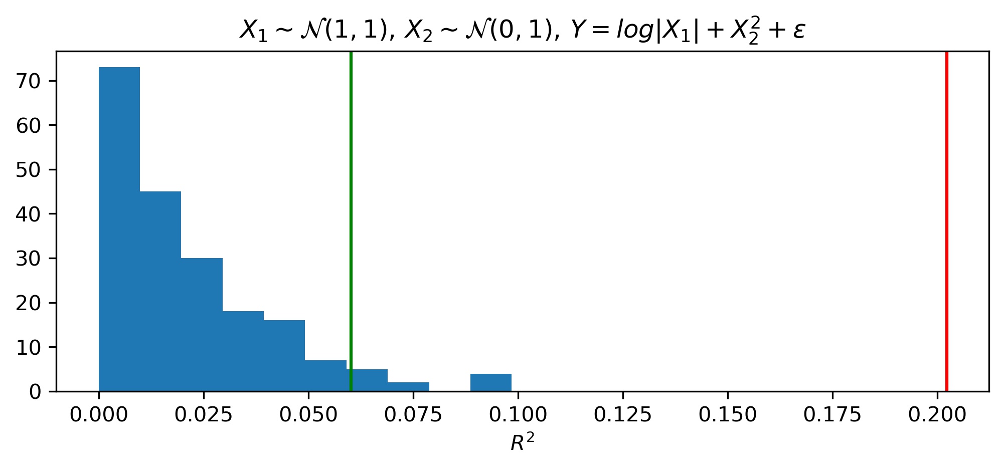
(a) Histogram of the distribution of generated $R^{2}$ using permutation of $y$ values. The model considered here is linear regression $\mathcal{F}_{\textrm{LR}}$. The sample size is 100. The red line denotes the observed $R^{2}$ for the true pairings of $X$ and $Y$, the green line denotes the 95%-quantile of the empirical distribution of $R^{2}$ (approximation using 200 permutations).

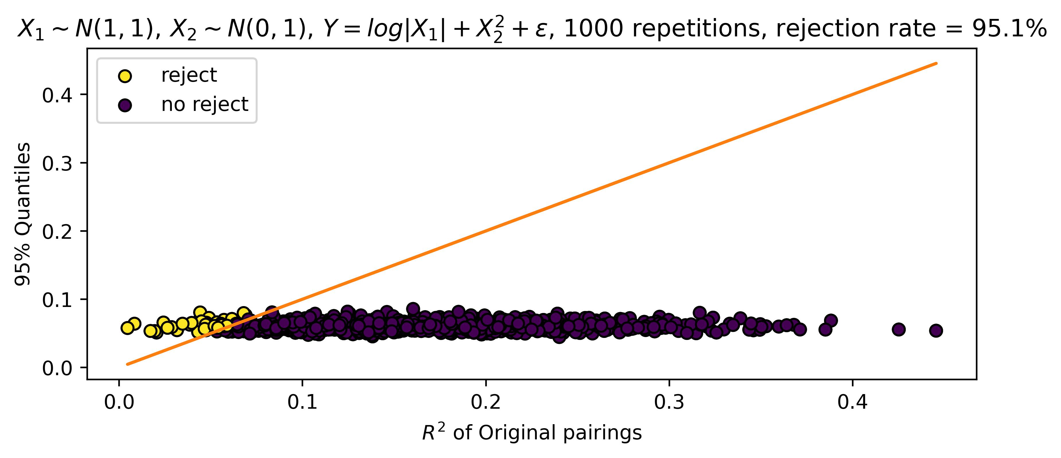
(b) Scatterplot of the $R^{2}$ values for the original pairings against the 95% quantiles of the empirical distribution of $R^{2}$. The orange line shows the identity function.

Figure 3: Results of the permutation test for $\mathcal{F}_{\textrm{LR}}$ with data generated in a following manner $X_{1}\sim\mathcal{N}(1,1),X_{2}\sim\mathcal{N}(0,1)$ and $Y=\log|X_{1}|+X_{2}^{2}+\epsilon$, where $\epsilon\sim\mathcal{N}(0,1)$.

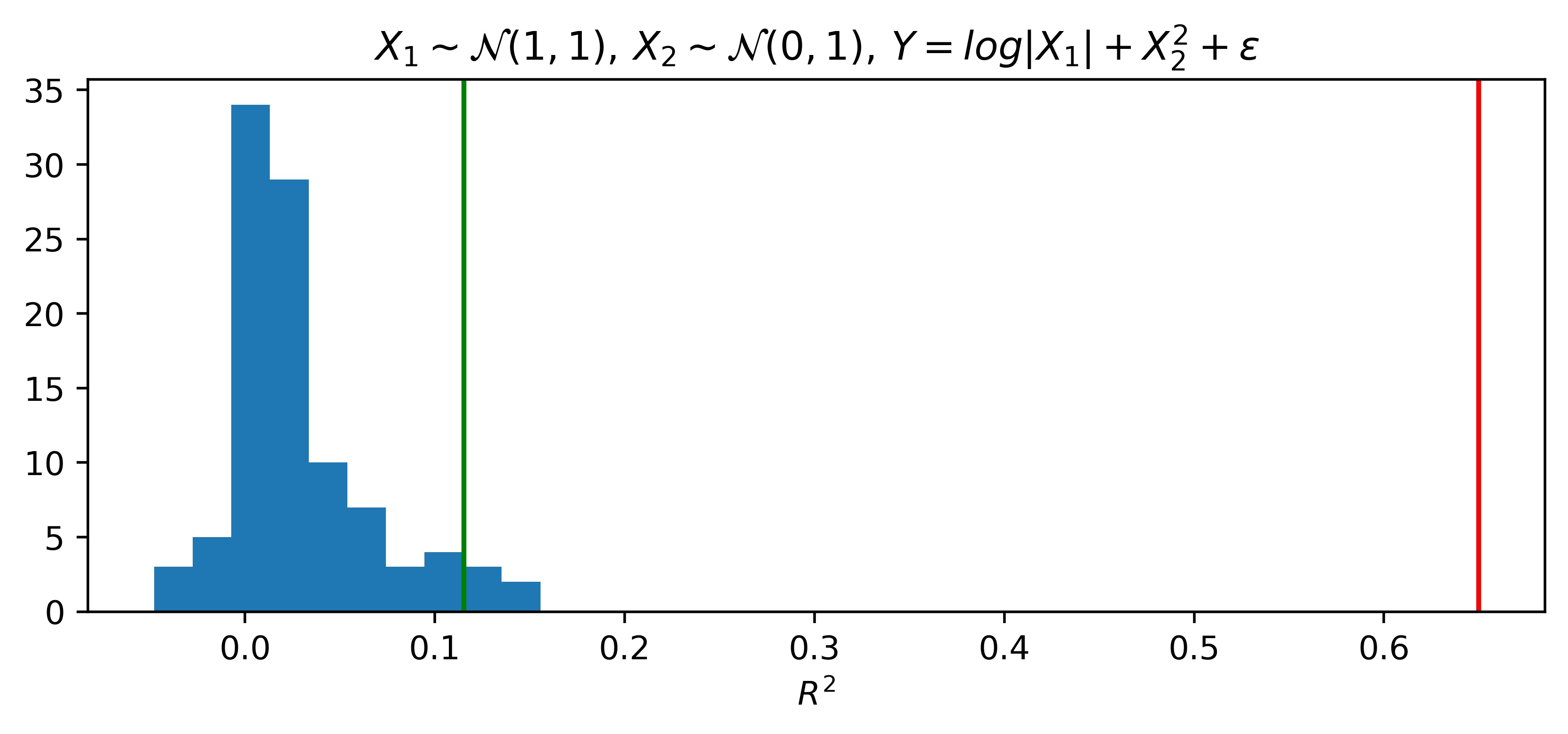
(a) Histogram of the distribution of generated $R^{2}$ using permutation of $y$ values. The model considered here is a 3-layered neural net $\mathcal{F}_{\textrm{NN}}(30,30,30)$. The sample size is 100. The red line denotes the observed $R^{2}$ for the true pairings of $X$ and $Y$, the green line denotes the 95%-quantile of the empirical distribution of $R^{2}$ (approximation using 200 permutations).

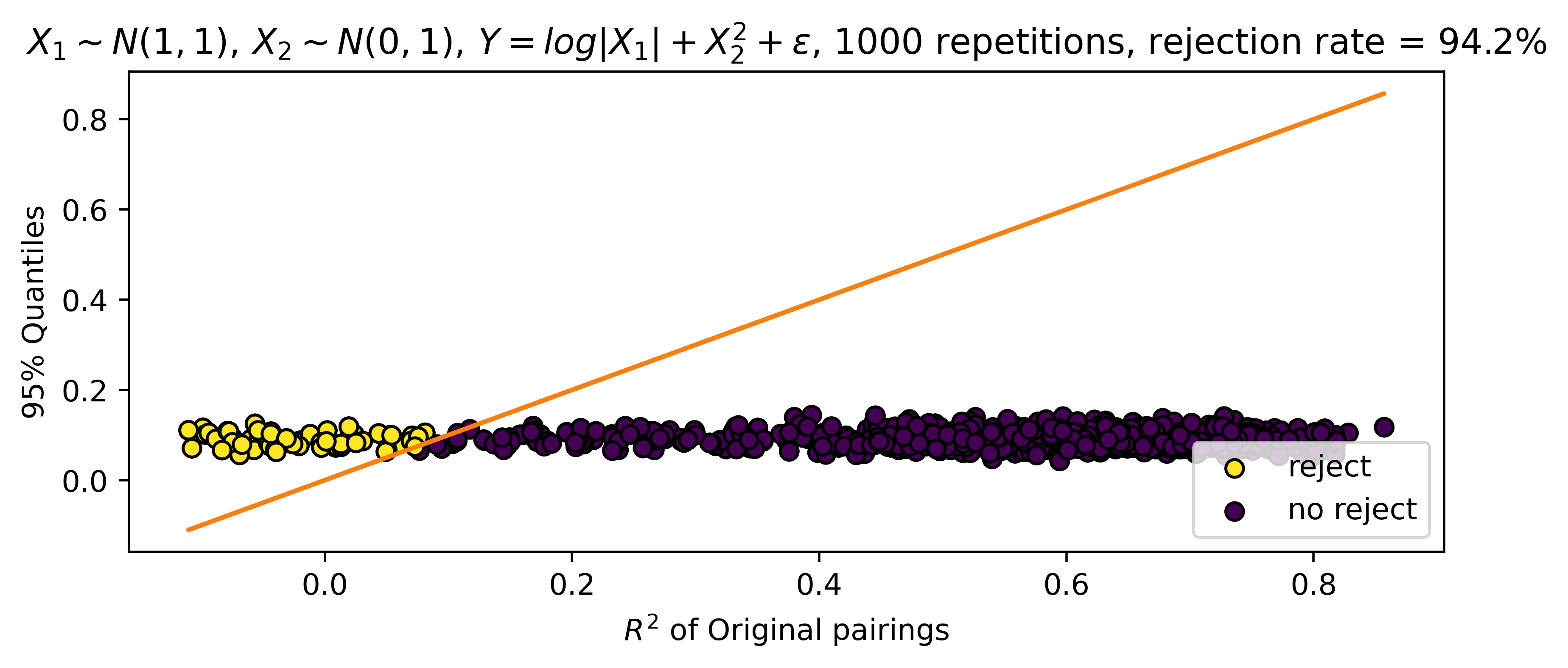
(b) Scatterplot of the $R^{2}$ values for the original pairings against the 95% quantiles of the empirical distribution of $R^{2}$. The orange line shows the identity function.

Figure 4: Results of the permutation test for $\mathcal{F}_{\textrm{NN}(30,30,30)}$ with data generated in a following manner $X_{1}\sim\mathcal{N}(1,1),X_{2}\sim\mathcal{N}(0,1)$ and $Y=\log|X_{1}|+X_{2}^{2}+\epsilon$, where $\epsilon\sim\mathcal{N}(0,1)$.

For the remaining scenarios in this section, we consider only the linear regression model $\mathcal{F}_{\textrm{LR}}$. We inspect the influence of changing the distribution slightly in the test in order to ensure the statistical analysis using the test is reliable and accurate. For $a\in\mathbb{R}$ let $X_{1}\sim\mathcal{N}(a,1),X_{2}\sim\mathcal{N}(0,0.1)$ be independent and $Y=\log|X_{1}|+X_{2}^{2}+\epsilon$, where $\epsilon\sim\mathcal{N}(0,0.1)$ is the noise. Consider a sample of size $100$. Note that the variance of $X_{2}$ has been decreased in comparison to the previous example. Only for values of $a$ close to 0, the null hypothesis is not rejected (fig. 5(a)). This makes sense, since the logarithm changes most rapidly close to $0$ and for those arguments it is difficult to fit a linear function which describes this relationship well. This pattern is the same with average rejection rate of $H_{0}$ when repeating the experiment 100 times for each value of $a$, see fig. 5(b). For values of $a$ greater than 0.6, the $H_{0}$ is almost never rejected. When the variance of $X_{2}$ increases to 0.5, the null hypothesis is no longer rejected for some values of $a$ larger than 5 (fig. 6). This particular case shows the influence of available information on rejecting the null hypothesis. The less informative predictors are the more likely it is not to reject the null hypothesis; we can see that as the parameter $a$ increases, the $\log|X_{1}|$ becomes flatter slowly losing its predictive value. Meanwhile, the influence of $X_{2}^{2}$ on the value of $Y$ increases and given that the model can only predict linearly in $X_{2}$, the power of the test decreases.

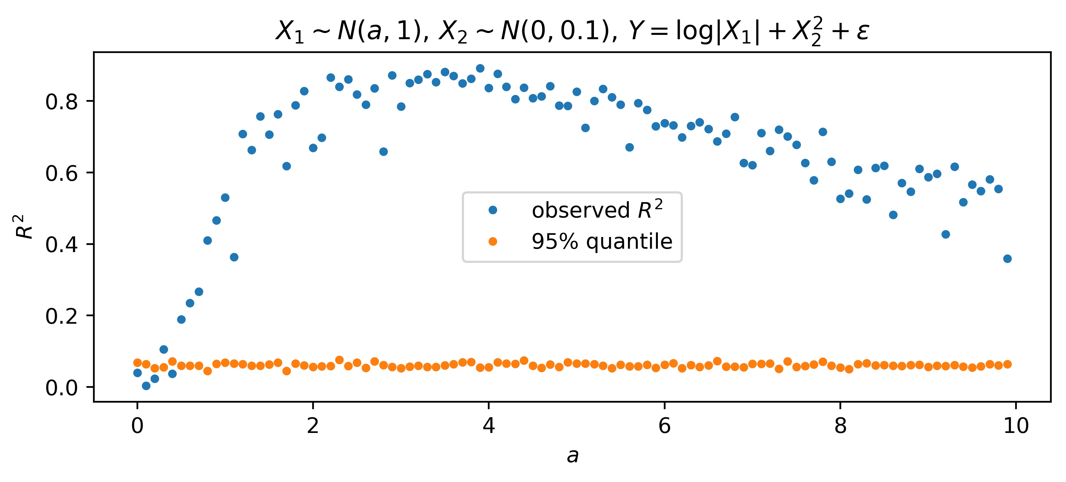
(a) The plot shows the results of performing the permutation test for linear regression model $\mathcal{F}_{\textrm{LR}}$. The sample size is 100. The blue dots show the observed $R^{2}$ and the orange dots show the 95% quantile of the empirical distribution of generated $R^{2}$ (approximation using 200 permutations). The test has been performed for values of $a$ ranging between 0 and 10.

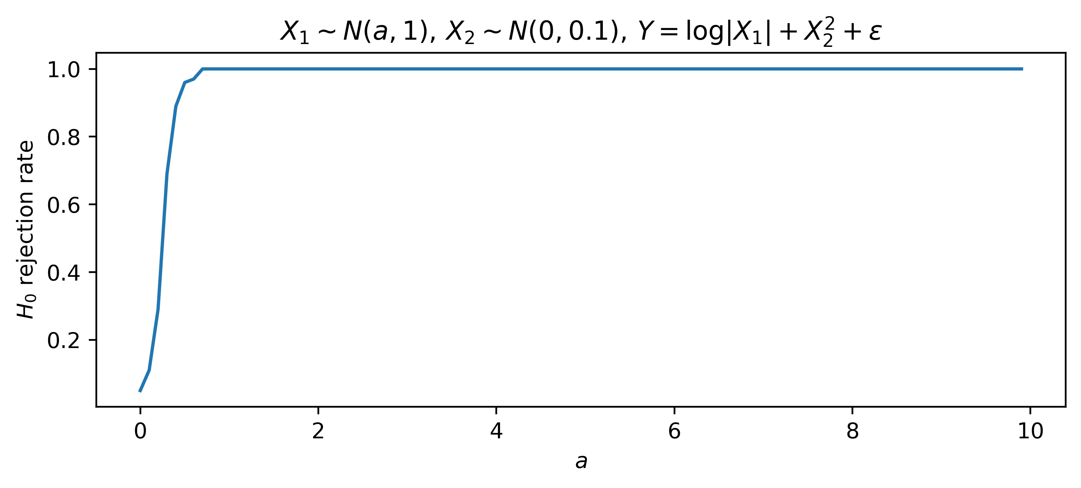
(b) Average rejection rate of $H_{0}$ with parameter $a$ varying from $0$ to $1$. For each $a$ 100 repetitions were made.

Figure 5: Results of the permutation test for $\mathcal{F}_{\textrm{LR}}$ with data generated in a following manner $X_{1}\sim\mathcal{N}(a,1),X_{2}\sim\mathcal{N}(0,0.1)$ and $Y=\log|X_{1}|+X_{2}^{2}+\epsilon$, where $\epsilon\sim\mathcal{N}(0,0.1)$.

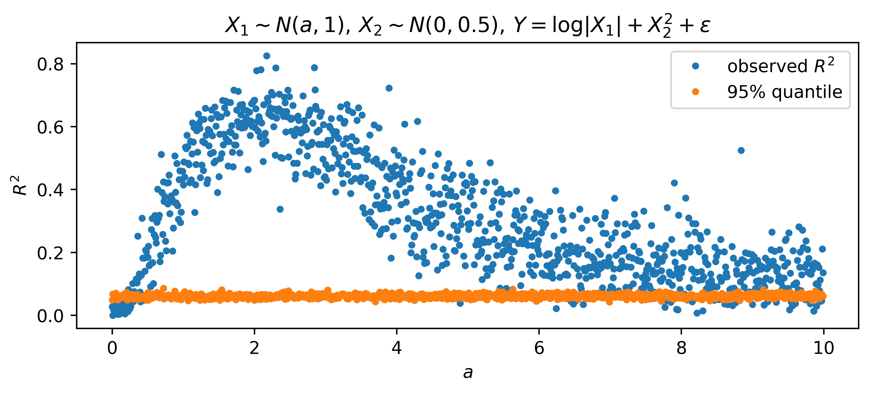
(a) The plot shows the results of performing the permutation test for linear regression model $\mathcal{F}_{\textrm{LR}}$. The sample size is 100. The blue dots show the observed $R^{2}$ and the orange dots show the 95% quantile of the empirical distribution of generated $R^{2}$ (approximation using 200 permutations). The test has been performed for values of $a$ ranging between 0 and 10.

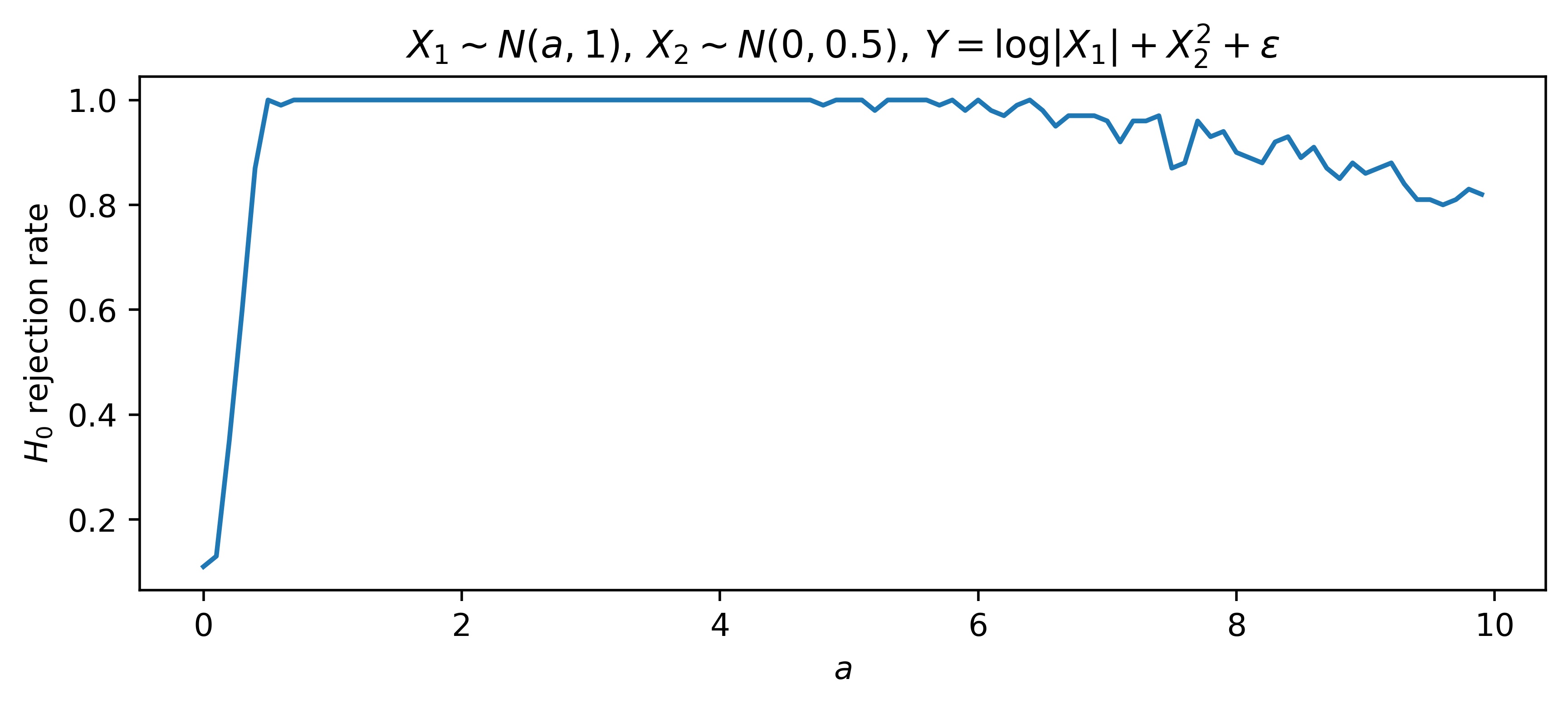
(b) Average rejection rate of $H_{0}$ with parameter $a$ varying from $0$ to $10$. For each $a$ 100 repetitions were made.

Figure 6: Results of the permutation test for $\mathcal{F}_{\textrm{LR}}$ with data generated in a following manner $X_{1}\sim\mathcal{N}(a,1),X_{2}\sim\mathcal{N}(0,0.5)$ and $Y=\log|X_{1}|+X_{2}^{2}+\epsilon$, where $\epsilon\sim\mathcal{N}(0,0.1)$.

Fig. 7 and 8 show explicitly the influence of the sample size on the test’s capability to reject $H_{0}$ for the linear regression model $\mathcal{F}_{\textrm{LR}}$. In the case when $H_{0}$ is true (fig. 7), the null hypothesis is rejected at a rate of 2-8% on average regardless of the sample size. In the case when $H_{0}$ is false (fig. 8), specifically with $Y=\log(X)+\epsilon$ for $\epsilon\sim\mathcal{N}(0,1)$, the null hypothesis is rejected much less for smaller sample sizes and the rejection rate increases as the sample size increases reaching close to 95% at sample size 300. We can conclude that the power of our test increases until the sample size of around 300, at which point the type II error is particularly low. Meanwhile, the rejection of a true null hypothesis is rare, even for the smallest of sample sizes.

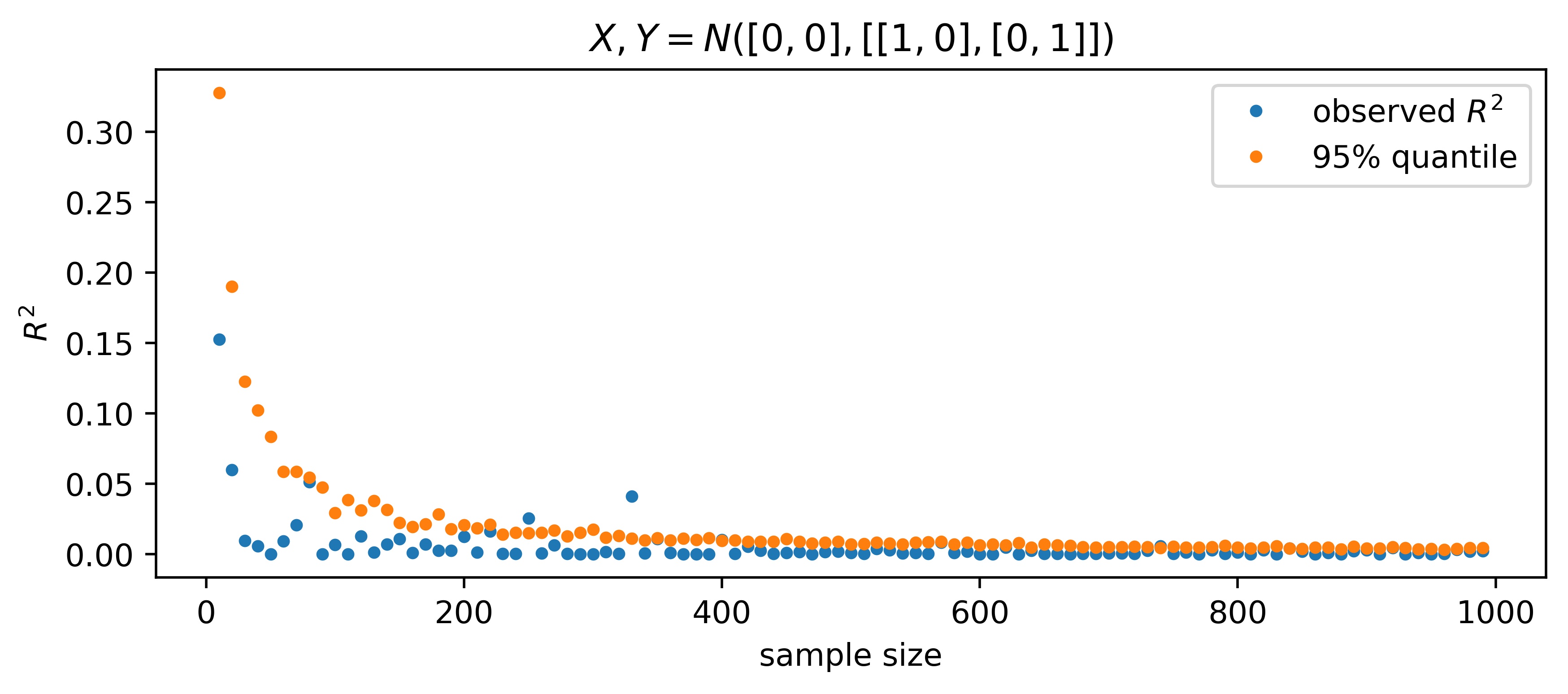
(a) The plot shows the results of performing the permutation test for linear regression model $\mathcal{F}_{\textrm{LR}}$. The blue dots show the observed $R^{2}$ and the orange dots show the 95% quantile of the empirical distribution of generated $R^{2}$ (approximation using 200 permutations). The test has been performed for sample sizes ranging between 10 and 1000.

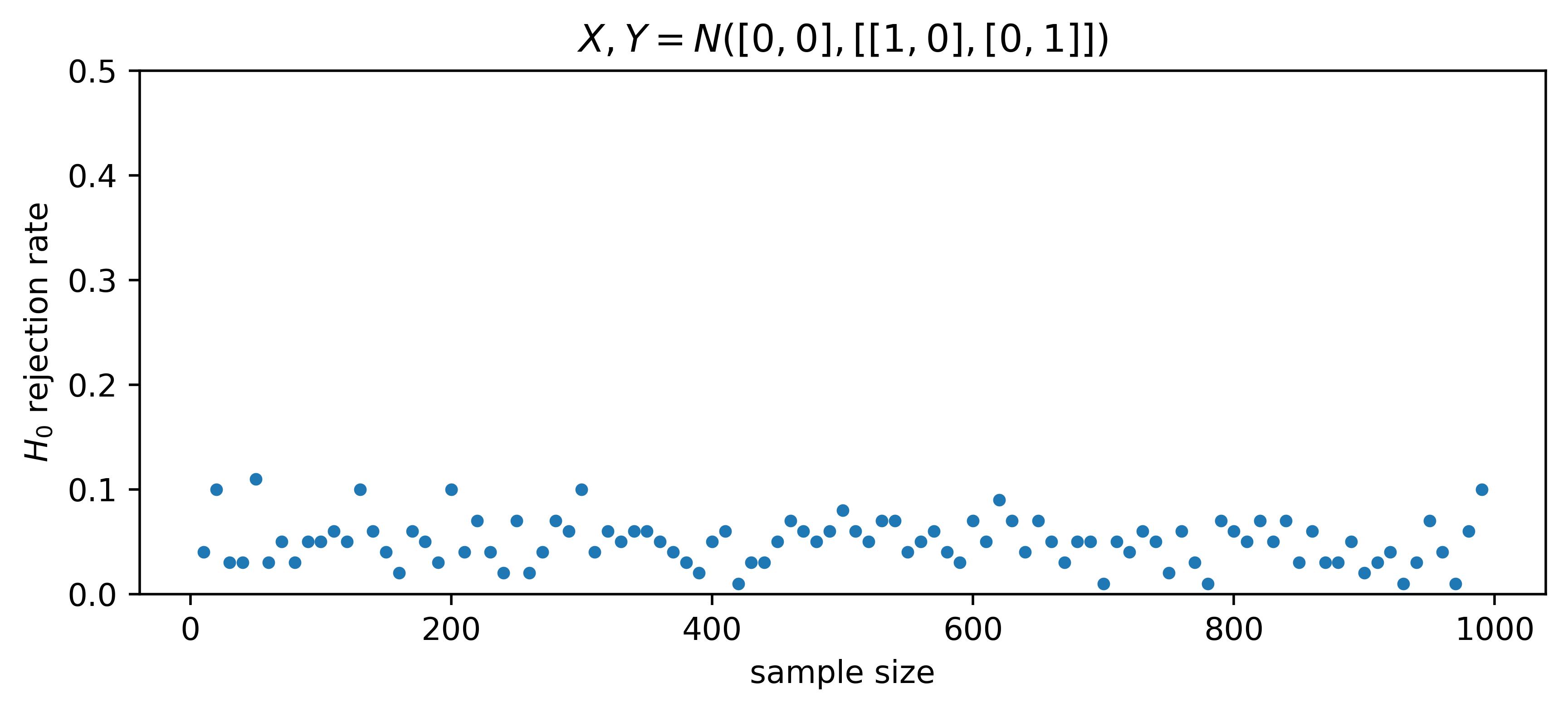
(b) Average rejection rate of $H_{0}$ with sample size varying from $10$ to $1000$. For each sample size 100 repetitions were made.

Figure 7: Results of the permutation test for $\mathcal{F}_{\textrm{LR}}$ with data generated in a following manner $X,Y\sim N(\mu,\Sigma)$, $\mu=\begin{bmatrix}0\\ 0\end{bmatrix}$ and $\sigma=\begin{bmatrix}1&0\\ 0&1\end{bmatrix}$.

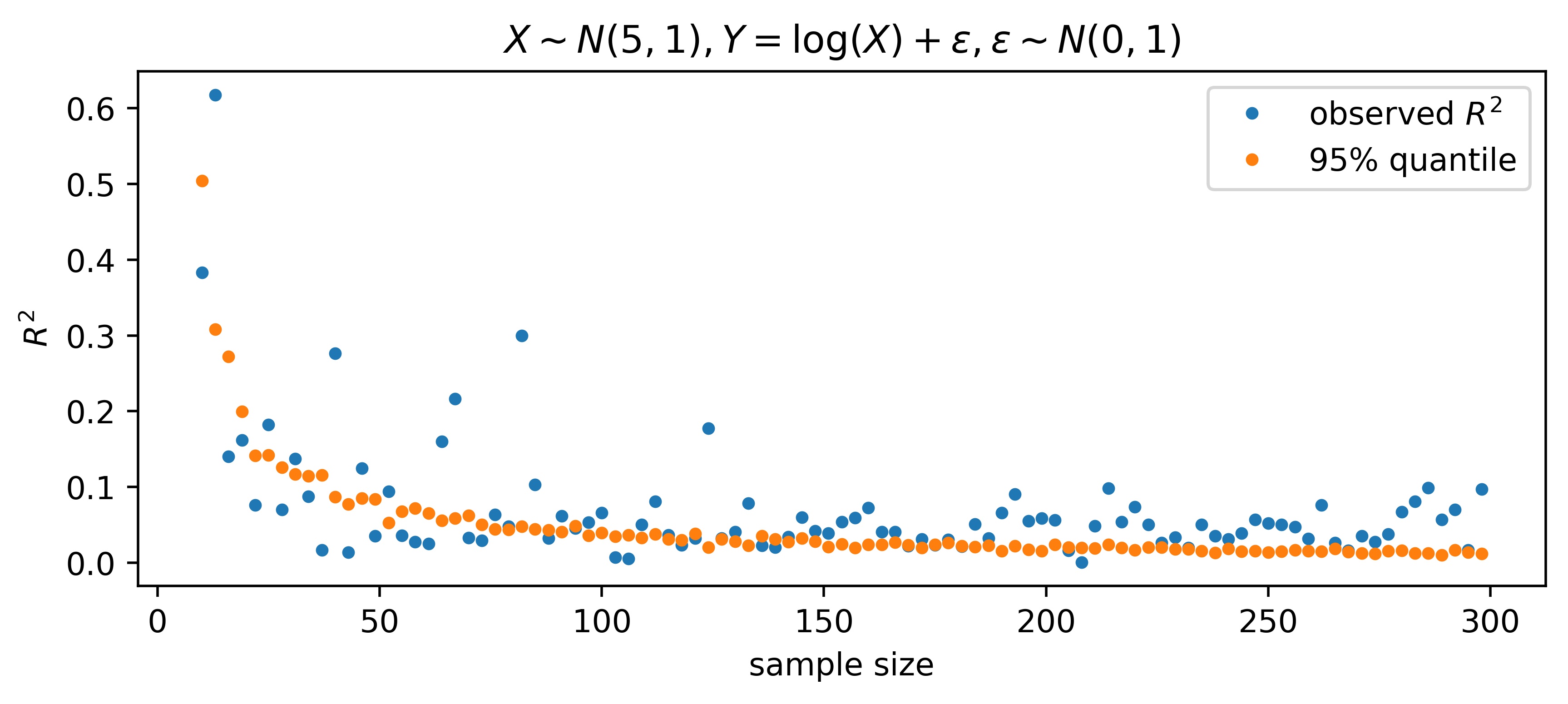
(a) The plot shows the results of performing the permutation test for linear regression model $\mathcal{F}_{\textrm{LR}}$. The blue dots show the observed $R^{2}$ and the orange dots show the 95% quantile of the empirical distribution of generated $R^{2}$ (approximation using 200 permutations). The test has been performed for sample sizes ranging between 10 and 300.

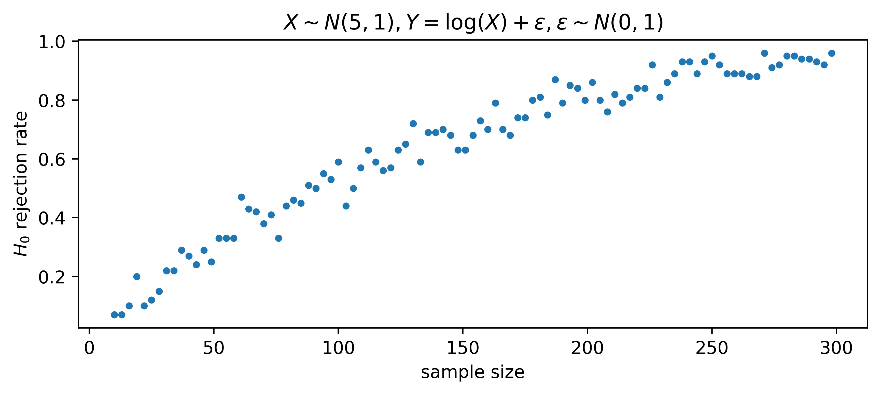
(b) Average rejection rate of $H_{0}$ with sample size varying from $10$ to $300$. For each sample size 100 repetitions were made.

Figure 8: Results of the permutation test for $\mathcal{F}_{\textrm{LR}}$ with data generated in a following manner $X\sim\mathcal{N}(5,1)$ and $Y=\log|X|+\epsilon$, where $\epsilon\sim\mathcal{N}(0,1)$.

Using the bivariate normal distribution with varying correlation, we can empirically detect the point at which the test rejects $H_{0}$ for the linear regression model $\mathcal{F}_{\textrm{LR}}$ as the variables become more and more dependent. Let $0\leq\rho\leq 1$ and $X,Y\sim N(\mu,\Sigma)$, such that

$$\mu=\begin{bmatrix}0\\ 0\end{bmatrix},\Sigma=\begin{bmatrix}1&\rho\\ \rho&1\end{bmatrix}.$$

Fig. 9 shows that as the correlation reaches 0.3, the test starts to reject $H_{0}$ almost always in case of sample size $n=100$. We conclude that for sample size $n=100$, the dependence is only detectable reliably by the test when the correlation between variables is greater than 0.3. This particular example shows that for a given sample size a certain threshold of correlation exists at which the test starts to reject the null hypothesis. As the correlation increases the rejection becomes more and more likely for a given sample size.

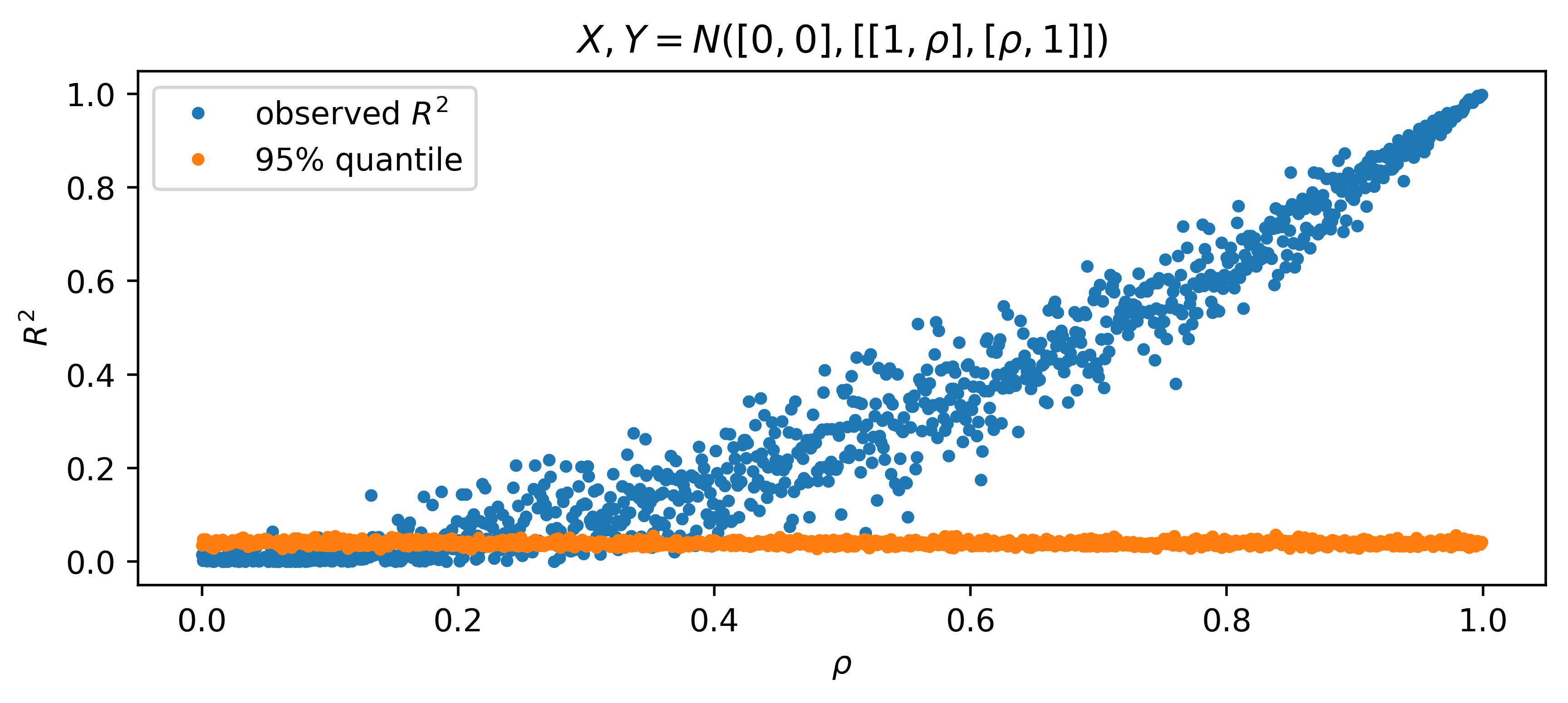
(a) The plot shows the results of performing the permutation test for linear regression model $\mathcal{F}_{\textrm{LR}}$. The sample size is 100. The blue dots show the observed $R^{2}$ and the orange dots show the 95% quantile of the empirical distribution of generated $R^{2}$ (approximation using 200 permutations). The test has been performed for values of correlation $\rho$ ranging between 0 and 1.

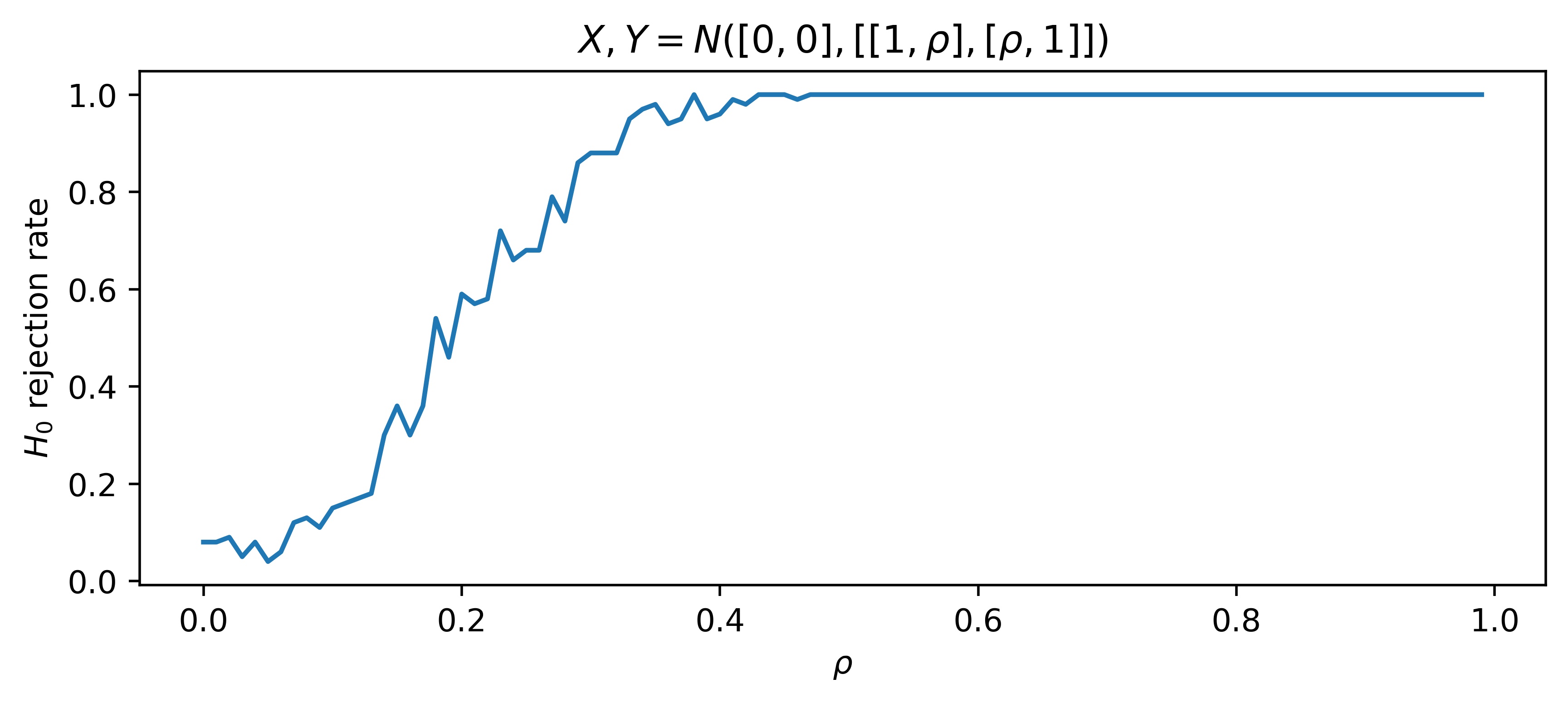
(b) Average rejection rate of $H_{0}$ with parameter $\rho$ varying from $0$ to $1$. For each $\rho$ 100 repetitions were made.

Figure 9: Results of the permutation test for $\mathcal{F}_{\textrm{LR}}$ with data generated in a following manner $X,Y\sim N(\mu,\Sigma)$, $\mu=\begin{bmatrix}0\\ 0\end{bmatrix}$ and $\Sigma=\begin{bmatrix}1&\rho\\ \rho&1\end{bmatrix}$.

Lastly, we present a comparison of our permutation test with a permutation test found in [25]. This is also a test for no effect, but specifically in the linear regression model. Its formulation requires a sample of $n$ i.i.d. observations $\{(X_{1},Y_{1}),\dots,(X_{n},Y_{n})\}$ from a bivariate variable $(X,Y)$. We assume that the variables are linked by a linear regression $\mathbb{E}(Y|X=x)=\alpha+\beta\cdot x$, where $\alpha,\beta\in\mathbb{R}$. The null hypothesis considered for this test is $\beta=0$, under the assumption that responses $Y_{i}$ can be permuted with respect to covariate $X$. The test statistic is $T^{*}_{\beta}=\sum_{i}X_{i}Y_{i}$ and the permutation of $Y_{i}$ is used when approximating the distribution of the test statistic under $H_{0}$. We refer to this test as the permutation test for linear regression after the naming convention in [25]. Note that in practice the only difference between our approaches is the choice of test statistic. In their case, the choice of the test statistic is driven by the null hypothesis. In our test, the test statistic can be chosen freely as long as it can be calculated using the sample $\{(f(x_{i}),y_{i})\}_{i}$, which technically means we could use $T^{\ast}_{\beta}$ as the test statistic. In that sense, we can view our test as the generalization of the test for linear regression.

We continue using bivariate normal variables $X$ and $Y$. We compare the average rejection rate of $H_{0}$ for both tests with parameter $\rho$ varying from $0$ to $1$. Fig. 10 shows the comparison between the tests. For sample size $n=100$, the permutation test for linear regression detects the dependence for a slightly smaller $\rho$ than our permutation test, but both reach the rejection rate of 1 at $\rho\approx 0.4$. We conclude that a context-specific test statistic, in this case $T^{\ast}_{\beta}$, outperforms more general statistic. At the same time, our test can use $T^{\ast}_{\beta}$ as the test statistic.

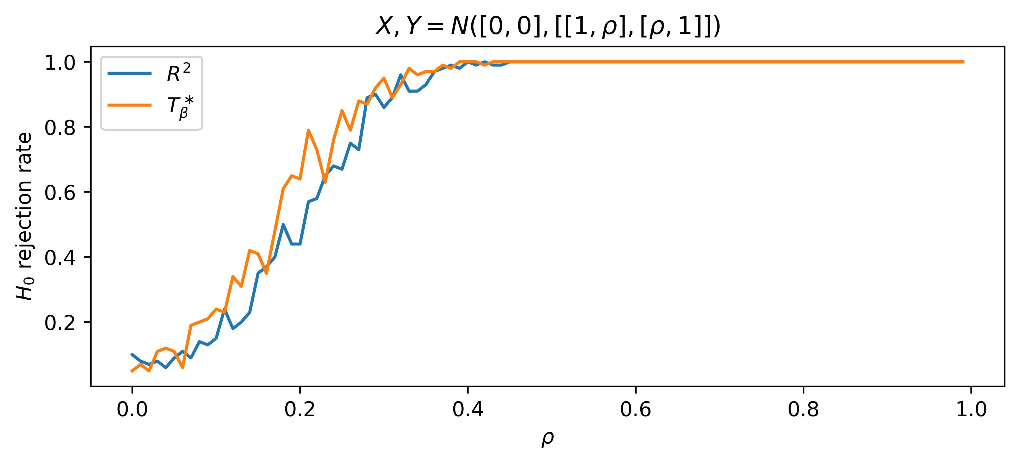
Figure 10: Average rejection rate of $H_{0}$ with parameter $\rho$ varying from $0$ to $1$. For each $\rho$ 100 repetitions were made. Two different tests were considered. Blue line was generated using $R^{2}$ as the test statistic, while the orange line was generated using $T^{\ast}_{\beta}$ as the test statistic.

3.2 Tennis serve dataset

This section concerns an application of the permutation test to a tennis serve dataset. Seven professional athletes wearing inertial measurement units (IMUs) performed tennis serves. Each athlete followed a protocol of first and second serves. Sensors were placed on 4 body parts: lower and upper arms, trunk and pelvis as can be seen in fig. 11. Each IMU contained a triaxial accelerometer and triaxial gyroscope. The data consists of 7 uninterrupted time series of 24-dimensional data (4 body parts $\times$ 2 types of sensors $\times$ 3 axes). The dataset is further described in the Master thesis [13].

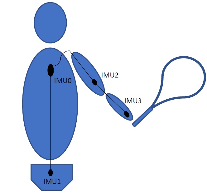
Figure 11: Segment model of right-handed player and racquet (back view, frontal plane).

Additionally, a dataset containing personal characteristics of the players and performance characteristics of each serve has been included. The personal characteristics are the sex, age, height and weight of the players. The performance characteristics are the ball velocity, an indication of whether the ball went in or out and the velocity-accuracy index (VA index). The VA index for a single serve was introduced and motivated in [20] and is defined as follows:

$$\textrm{VA index}=\frac{(\textrm{ball velocity (kph)})^{2}}{100}\times\frac{\textrm{achieved points}}{9},$$ (7)

where achieved points refer to the number of points assigned to a serve based on its closeness to a target area on the court (see fig. 12). The number of points assigned to a serve is based on a new Serve Tennis Test (STT) introduced in [31]. Originally, the point system was devised based on the ellipses in the serve box where aces were hit in male tennis matches during the Australian Open [32]. However, the system has been improved upon since then. The points are discrete. Nine points are given for hitting the center of the target area. Six and three points are assigned for areas further from the center. One point is assigned for a ball much further from the target area, but still a valid ball, while zero points are given to a serve which did go out. Each participant performed approximately 48 serves. In total, 29.6% of serves were faults (and as a result had a VA-index 0).

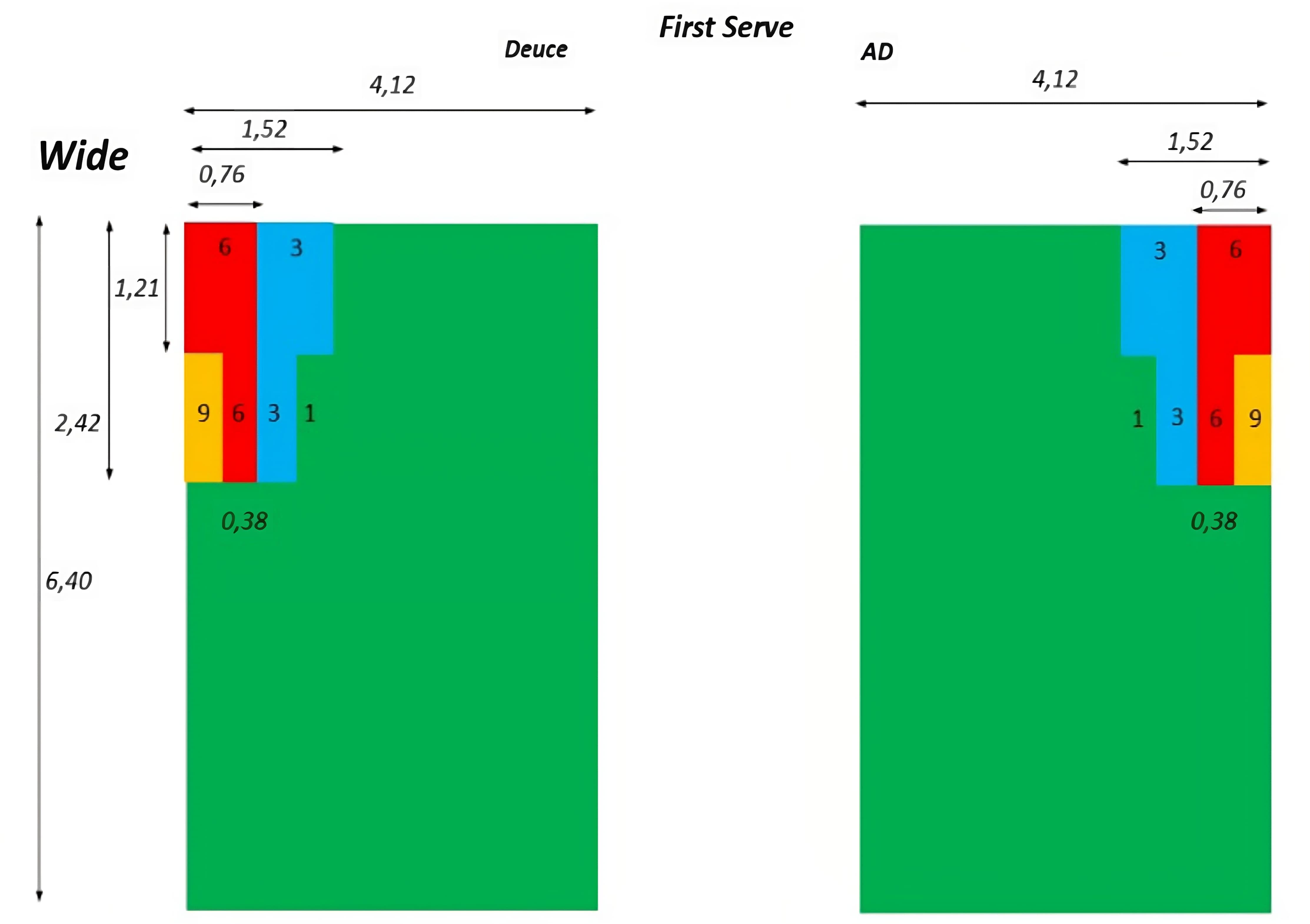
Figure 12: Target areas for the tennis serve. The scenario considered here is a serve in the wide direction. The points given on each target area correspond to the number of accuracy points needed to calculate the VA index of the serve.

We will use the tennis serve dataset in order to demonstrate an application of the permutation test to real life data. We will focus on the prediction of ball speed and VA-index prediction. The functional predictors have been transformed into vectors, using a Fourier basis representation, in order to be able to use the linear regression model $\mathcal{F}_{\textrm{LR}}$ and the neural net $\mathcal{F}_{\textrm{NN}}(300,300,300)$. The choice to use Fourier coefficients as predictors was the most natural way of incorporating information from the time series. First, a prediction of ball speed was considered. The permutation test rejected the null hypothesis in cases of both models as seen in fig. 13(a) and 13(b). The test rejects the null hypothesis for both models, although higher values of $R^{2}$ achieved by the neural net for the original pairings suggest greater capabilities of that model to detect the dependence.

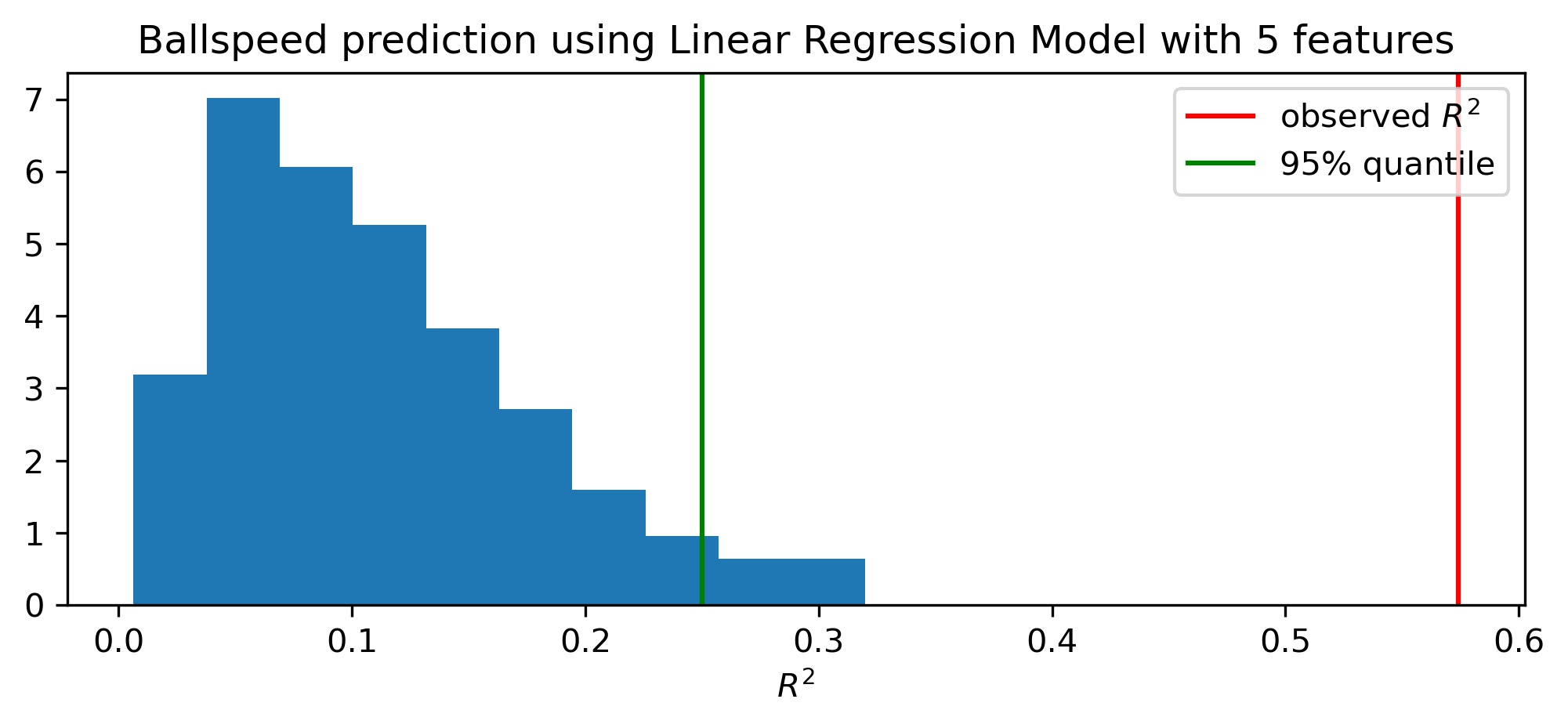
(a) Histogram of the distribution of generated $R^{2}$ using permutation of $y$ values. The sample size is 46. The red line denotes the observed $R^{2}$ for the true pairings of $X$ and $Y$, the green line denotes the 95%-quantile of the empirical distribution of $R^{2}$ (approximation using 200 permutations).

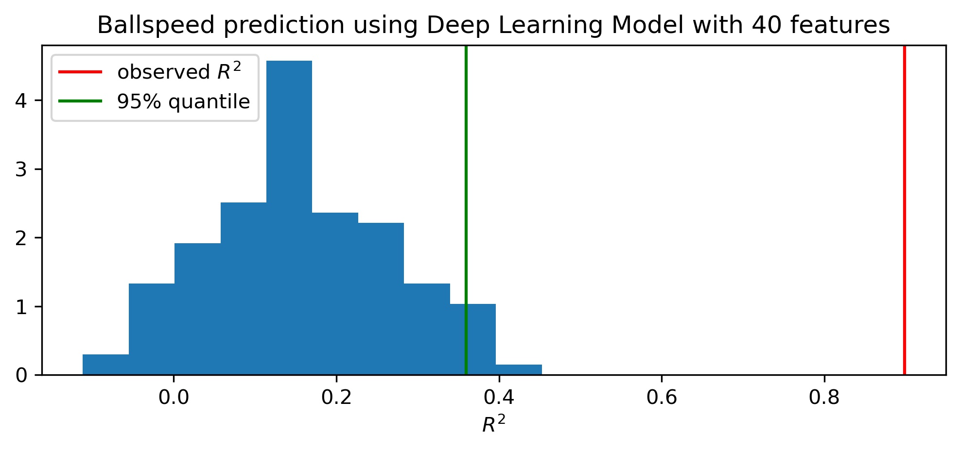
(b) Histogram of the distribution of generated $R^{2}$ using permutation of $y$ values. The sample size is 46. The red line denotes the observed $R^{2}$ for the true pairings of $X$ and $Y$, the green line denotes the 95%-quantile of the empirical distribution of $R^{2}$ (approximation using 200 permutations).

Figure 13: Results of the permutation test for the ball speed prediction using $\mathcal{F}_{\textrm{LR}}$ and $\mathcal{F}_{\textrm{NN}}(300,300,300)$.

In the case of prediction of the VA-index as defined in (7), the permutation test did not reject the null hypothesis for the linear regression model $\mathcal{F}_{\textrm{LR}}$ as well as for the neural net model $\mathcal{F}_{\textrm{NN}}(300,300,300)$. Fig. 14(a) shows results for the linear regression model and fig. 14(b) shows results for the neural net. The values of $R^{2}$ are quite low for both models and for many permutations of $y$-values the generated $R^{2}$ is much higher than the observed $R^{2}$ for the true pairings. These results convince us that a good prediction using the linear regression model or the neural net model is not possible at the moment. The issue may lie with the current size of the dataset or the number of serves per player or simply because the relation as can be described by the neural net is not strong. The fact that the number of Fourier coefficients used in this prediction was increased to achieve more favourable $R^{2}$ for the original pairings of $(x_{i},y_{i})$ (at least in the case of the deep learning model), shows how complex this task is and additional information is needed in the data to increase the $R^{2}$.

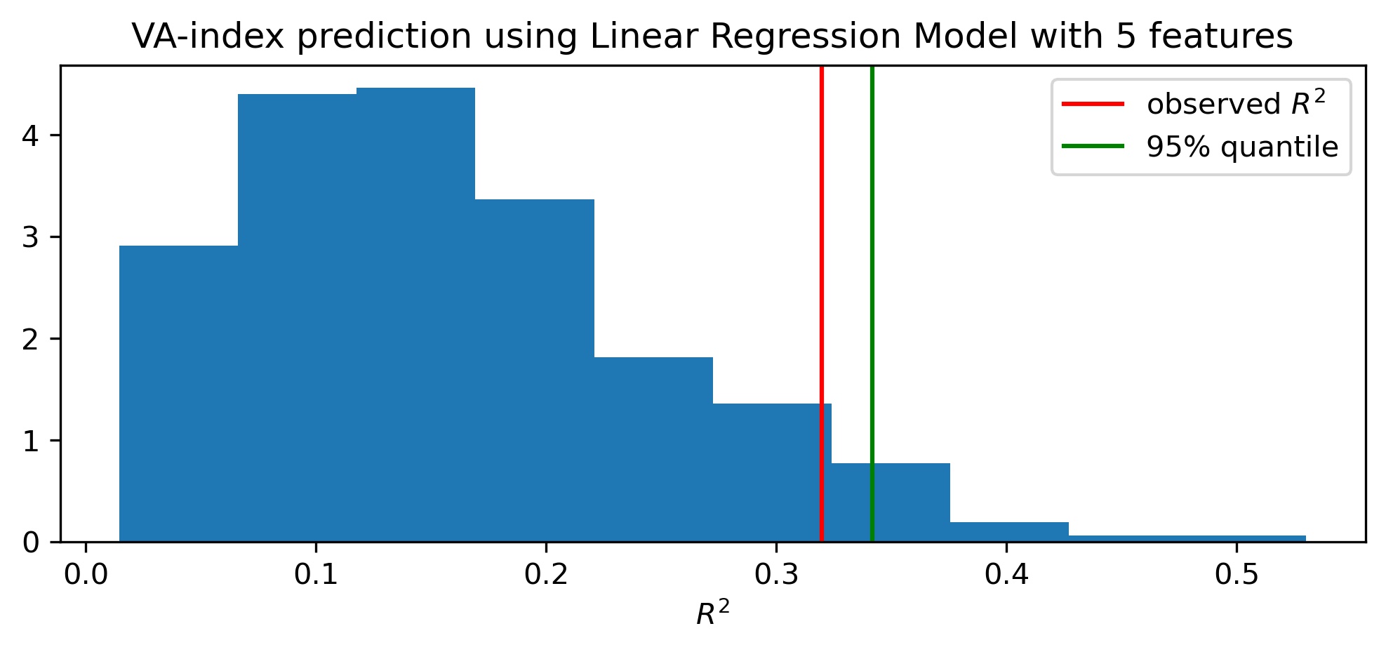
(a) Histogram of the distribution of generated $R^{2}$ using permutation of $y$ values. The sample size is 34. The red line denotes the observed $R^{2}$ for the true pairings of $X$ and $Y$, the green line denotes the 95%-quantile of the empirical distribution of $R^{2}$ (approximation using 200 permutations).

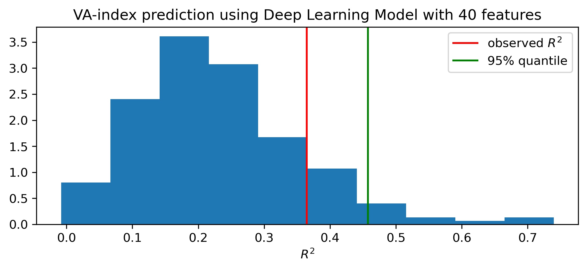
(b) Histogram of the distribution of generated $R^{2}$ using permutation of $y$ values. The sample size is 34. The red line denotes the observed $R^{2}$ for the true pairings of $X$ and $Y$, the green line denotes the 95%-quantile of the empirical distribution of $R^{2}$ (approximation using 200 permutations).

Figure 14: Results of the permutation test for the VA index prediction using $\mathcal{F}_{\textrm{LR}}$ and $\mathcal{F}_{\textrm{NN}}(300,300,300)$.

4 Conclusion and discussion

This paper concerns the theoretical foundations and the application of the permutation approach for testing whether a model can capture dependence structure between predictors and responses. The test is a tool to determine whether a model is able to fit the data better than pure noise. We are mostly interested whether $X$ has any effect on $Y$ and we pursue that interest with the help of a chosen, fixed model. The null hypothesis is formulated in terms of independence of $Y$ and $f(X)$ for all $f$ in the model and in this form cannot be found in previous literature. Proposition 2.1 allows us to consider the test as a permutation test formally and proposition 2.2 allows us to consider $R^{2}$ as a test statistic. This approach is data-centered and the results of the test depend on just one model without the need to directly compare between different models. We also do not require sample splitting thus the test can rely on the power of the whole sample size, which can be vital in datasets of smaller size. Our findings are supported through a simulation study, which highlights the performance of the test in various different dependence scenarios, as well as an application to the tennis serve dataset, which shows an application in real-life scenario. In this case, it gave evidence that a seemingly well-fitting model is not necessarily trustworthy. The prediction is either not possible with the given sensor data and model or a larger sample size is needed to predict the VA-index more accurately.

Declaration of interests

The authors declare that they have no known competing financial interests or personal relationships that could have appeared to influence the work reported in this paper.

Code availability

Custom code for simulation study can be found at: https://github.com/mgciszewski/credibility_2023.

Data availability

The data that support the findings of this study are available from the corresponding author upon request.

Funding

This work is part of the research programme CAS with project number P16-28 project 2, which is (partly)

financed by the Dutch Research Council (NWO).

References

- [1] M.J. Anderson and J. Robinson, Permutation tests for linear models, Aust. N. Z. J. Stat. 43 (2001), pp. 75–88. Available at https://doi.org/10.1111/1467-842X.00156.
- [2] R. Arboretti Giancristofaro and S. Bonnini, Moment-based multivariate permutation tests for ordinal categorical data, J. Nonparametr. Stat. 20 (2008), pp. 383–393. Available at https://doi.org/10.1080/10485250802195440.
- [3] R. Arboretti Giancristofaro and S. Bonnini, Some new results on univariate and multivariate permutation tests for ordinal categorical variables under restricted alternatives, Stat. Methods and Appl. 18 (2009), pp. 221–236. Available at https://doi.org/10.1007/s10260-008-0096-6.
- [4] R. Arboretti Giancristofaro, S. Bonnini, and F. Pesarin, A permutation approach for testing heterogeneity in two-sample categorical variables., Stat. and Comput. 19 (2009), pp. 209–216. Available at https://doi.org/10.1007/s11222-008-9085-8.
- [5] C.B. Bell and K.A. Doksum, Distribution-free tests of independence, Ann. Math. Statist. 38 (1967), pp. 429–446. Available at https://doi.org/10.1214/aoms/1177698959.
- [6] K.J. Berry, P.W. Mielke Jr., and H.W. Mielke, The Fisher-Pitman permutation test: an attractive alternative to the test, Psychol. Rep. 90 (2002), pp. 495–502. Available at https://doi.org/10.2466/pr0.2002.90.2.495.
- [7] R.J. Boik, The Fisher-Pitman permutation test: A non-robust alternative to the normal theory test when variances are heterogeneous, Br. J. Math. Stat. Psychol. 40 (1987), pp. 26–42. Available at https://doi.org/10.1111/j.2044-8317.1987.tb00865.x.
- [8] S. Bonnini and M. Borghesi, Relationship between mental health and socio-economic, demographic and environmental factors in the covid-19 lockdown period - a multivariate regression analysis, Mathematics (MDPI) 10 (2022), p. 3237. Available at https://doi.org/10.3390/math10183237.
- [9] H. Cardot, A. Goia, and P. Sarda, Testing for no effect in functional linear regression models, some computational approaches, Commun. Stat. Simul. Comput. 33 (2004), pp. 179–199. Available at https://doi.org/10.1081/SAC-120028440.
- [10] D. Commenges, Transformations which preserve exchangeability and application to permutation tests, J. Nonparametr. Stat. 15 (2003), pp. 171–185. Available at https://doi.org/10.1080/1048525031000089310.
- [11] C.J. DiCiccio and J.P. Romano, Robust permutation tests for correlation and regression coefficients, J. Am. Stat. Assoc. 112 (2017), pp. 1211–1220. Available at https://doi.org/10.1080/01621459.2016.1202117.
- [12] W. Duivesteijn and A. Knobbe, Exploiting false discoveries - statistical validation of patterns and quality measures in subgroup discovery, in Proc. 2011 IEEE 11th Int. Conf. Data Min., Vancouver, BC, Canada. IEEE, 2011, pp. 151–160.
- [13] E. Faneker, The kinetic chain and serve performance in elite tennis players (Master Research Project, Vrije Universiteit Amsterdam), 2021.
- [14] R.A. Fisher, Statistical methods for research workers, 1st ed., Oliver & Boyd, Edinburgh, Scotland, 1925.
- [15] P.I. Good, Extensions of the concept of exchangeability and their applications, J. Mod. Appl. Stat. Methods 1 (2002), pp. 243–247. Available at https://doi.org/10.22237/jmasm/1036110240.
- [16] S. Hahn and L. Salmaso, A comparison of different synchronized permutation approaches to testing effects in two-level two-factor unbalanced anova designs, Stat. Papers 58 (2017), pp. 123–146. Available at https://doi.org/10.1007/s00362-015-0690-2.
- [17] N.S. Hall, R. A. Fisher and his advocacy of randomization, J. Hist. Biol. 40 (2007), pp. 295–325. Available at https://doi.org/10.1007/s10739-006-9119-z.
- [18] Y. Huang, H. Xu, V. Calian, and J.C. Hsu, To permute or not to permute, Bioinform. 22 (2006), pp. 2244–2248. Available at https://doi.org/10.1093/bioinformatics/btl383.
- [19] A.D. Hutson and G.E. Wilding, Maintaining the exchangeability assumption for a two-group permutation test in the non-randomized setting, J. Appl. Stat. 39 (2012), pp. 1593–1603. Available at https://doi.org/10.1080/02664763.2012.661707.
- [20] N. Kolman, B. Huijgen, T. Kramer, M. Elferink-Gemser, and C. Visscher, The Dutch Technical-Tactical Tennis Test (D4T) for talent identification and development: psychometric characteristics, J. Hum. Kinet. 30 (2017), pp. 127–138. Available at https://doi.org/10.1515/hukin-2017-0012.
- [21] A.N. Kolmogorov, Foundations of the theory of probability, 2nd ed., Chelsea Publishing Company, New York, 1956.
- [22] O.E. Lee and T.M. Braun, Permutation tests for random effects in linear mixed models, Biometr. 68 (2012), pp. 486–493. Available at https://doi.org/10.1111/j.1541-0420.2011.01675.x.
- [23] J. Ludbrook and H. Dudley, Why permutation tests are superior to and tests in biomedical research, Am. Stat. 52 (1998), pp. 127–132. Available at https://doi.org/10.2307/2685470.
- [24] A. Oden and H. Wedel, Arguments for Fisher’s permutation test, Ann. Statist. 3 (1975), pp. 518–520. Available at https://doi.org/10.1214/aos/1176343082.
- [25] F. Pesarin and L. Salmaso, Permutation tests for complex data: theory, applications and software, 1st ed., John Wiley & Sons, Chichester, UK, 2010.
- [26] E. Pitman, Significance tests which may be applied to samples from any populations, Suppl. J. Royal Stat. Soc. 4 (1937), pp. 119–130. Available at https://doi.org/10.2307/2984124.
- [27] E. Pitman, Significance tests which may be applied to samples from any populations. ii. the correlation coefficient test., Suppl. J. Royal Stat. Soc. 4 (1937), pp. 225–232. Available at https://doi.org/10.2307/2983647.
- [28] J.P. Romano, On the behavior of randomization tests without a group invariance assumption, J. Am. Stat. Assoc. 85 (1990), pp. 686–692. Available at https://doi.org/10.2307/2290003.
- [29] R.L. Schmoyer, Permutation tests for correlation in regression errors, J. Am. Stat. Assoc. 89 (1994), pp. 1507–1516. Available at https://doi.org/10.2307/2291013.
- [30] C.J.F. ter Braak, Predictor versus response permutation for significance testing in weighted regression and redundancy analysis, J. Stat. Comp. Simul. 92 (2021), pp. 2041–2059. Available at https://doi.org/10.1080/00949655.2021.2019256.
- [31] T. van Dijk, T.A. Leenen, B. van Trigt, A. Hoekstra, and M.M. Hoozemans, Development, construct validity and test-retest reliability of a Serve Tennis Test (STT) in elite tennis, (unpublished manuscript) .
- [32] D. Whiteside and M. Reid, Spatial characteristics of professional tennis serves with implications for serving aces: A machine learning approach, J. Sports Sci. 35 (2017), pp. 648–654. Available at https://doi.org/10.1080/02640414.2016.1183805.
- [33] A.M. Winkler, G.R. Ridgway, M.A. Webster, S.M. Smith, and T.E. Nichols, Permutation inference for the general linear model, Neuroimage 92 (2014), pp. 381–397. Available at https://doi.org/10.1016/j.neuroimage.2014.01.060.
- [34] A.M. Winkler, M.A. Webster, D. Vidaurre, T.E. Nichols, and S.M. Smith, Permutation inference for the general linear model, Neuroimage 123 (2015), pp. 253–268. Available at https://doi.org/10.1016/j.neuroimage.2015.05.092.
- [35] S. Zhang, The split sample permutation -tests, Neuroimage 139 (2009), pp. 3512–3524. Available at https://doi.org/10.1016/j.jspi.2009.04.004.