Neighboring Words Affect Human Interpretation of Saliency Explanations

Abstract

Word-level saliency explanations (“heat maps over words”) are often used to communicate feature-attribution in text-based models. Recent studies found that superficial factors such as word length can distort human interpretation of the communicated saliency scores. We conduct a user study to investigate how the marking of a word’s neighboring words affect the explainee’s perception of the word’s importance in the context of a saliency explanation. We find that neighboring words have significant effects on the word’s importance rating. Concretely, we identify that the influence changes based on neighboring direction (left vs. right) and a-priori linguistic and computational measures of phrases and collocations (vs. unrelated neighboring words). Our results question whether text-based saliency explanations should be continued to be communicated at word level, and inform future research on alternative saliency explanation methods.

1 Introduction

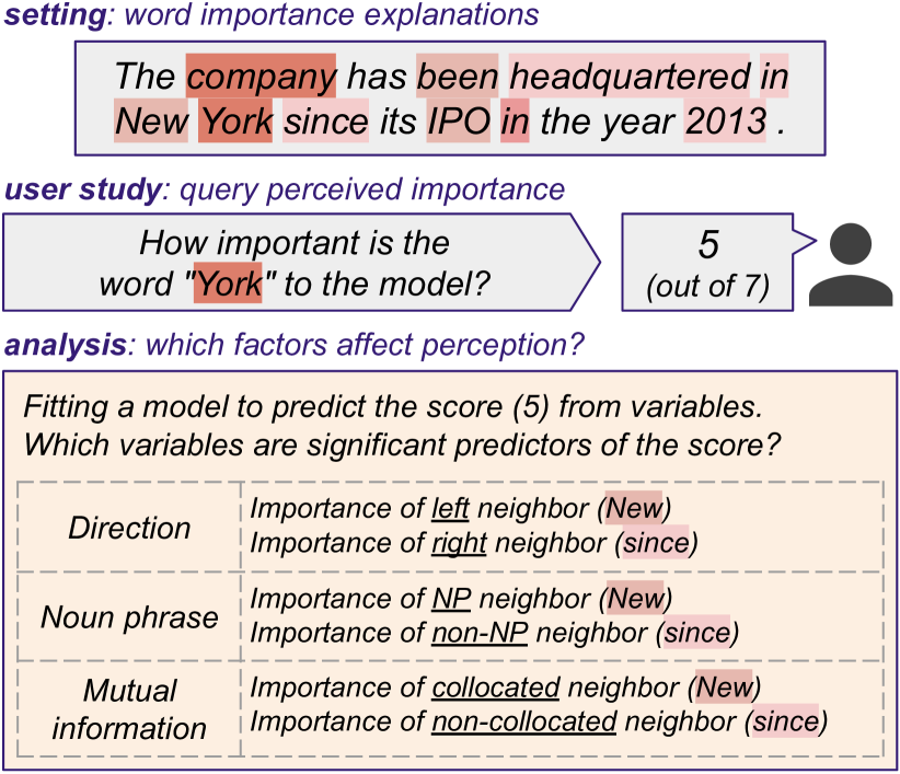
Figure 1: Illustration of the user study. We ask laypeople to rate the perceived importance of words following a word-importance explanation (grey). Then we analyze the effect of the importance of neighboring words on this interpretation, conditioned on the relationship between the words across various measures (orange).

In the context of explainability methods that assign importance scores to individual words, we are interested in characterizing the effect of phrase-level features on the perceived importance of a particular word: Text is naturally constructed and comprehended in various levels of granularity that go beyond the word-level Chomsky (1957); Xia (2018). For example (Figure 1), the role of the word “York” is contextualized by the phrase “New York” that contains it. Given an explanation that attributes importance to “New” and “York” separately, what is the effect of the importance score of “New” on the explainee’s understanding of the importance “York”? Our study investigates this question.

Current feature-attribution explanations in NLP mostly operate at word-level or subword-level Madsen et al. (2023); Arras et al. (2017); Ribeiro et al. (2016); Carvalho et al. (2019). Previous work investigated the effect of word and sentence-level features on subjective interpretations of saliency explanations on text Schuff et al. (2022)—finding that features such as word length and frequency bias users’ perception of explanations (e.g., users may assign higher importance to longer words).

It is not trivial for an explanation of an AI system to successfully communicate the intended information to the explainee Miller (2019); Dinu et al. (2020); Fel et al. (2021); Arora et al. (2021). In the case of feature-attribution explanations Burkart and Huber (2021); Tjoa and Guan (2021), which commonly appear in NLP as explanations based on word importance Madsen et al. (2023); Danilevsky et al. (2020), we must understand how the explainee interprets the role of the attributed inputs on model outputs Nguyen et al. (2021); Zhou et al. (2022). Research shows that it is often an error to assume that explainees will interpret explanations “as intended” Gonzalez et al. (2021); Ehsan et al. (2021).

The study involves two phases (Figure 1). First, we collect subjective self-reported ratings of importance by laypeople, in a setting of color-coded word importance explanations of a fact-checking NLP model (Section 2, Figure 2). Then, we fit a statistical model to map the importance of neighboring words to the word’s rating, conditioned on various a-priori measures of bigram constructs, such as the words’ syntactic relation or the degree to which they collocate in a corpus Kolesnikova (2016).

We observe significant effects (Section 4) for: 1. left-adjacency vs. right-adjacency; 2. the difference in importance between the two words; 3. the phrase relationship between the words (common phrase vs. no relation). We then deduce likely causes for these effects from relevant literature (Section 5). We are also able to reproduce results by Schuff et al. (2022) in a different English language domain (Section 3). We release the collected data and analysis code.

We conclude that laypeople interpretation of word importance explanations in English can be biased via neighboring words’ importance, likely moderated by reading direction and phrase units of language. Future work on feature-attribution should investigate more effective methods of communicating information Mosca et al. (2022); Ju et al. (2022), and implementations of such explanations should take care not to assume that human users interpret word-level importance objectively.

2 Study Specification

Our analysis has two phases: Collecting subjective interpretations of word-importances from laypeople, and testing for significant influence in various properties on the collected ratings—in particular, properties of adjacent words to the rated word.

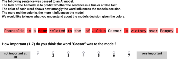
Figure 2: Screenshot of the rating interface.

2.1 Collecting Perceived Importance

We ask laypeople to rate the importance of a word within a feature-importance explanation (Figure 2). The setting is based on Schuff et al. (2022), with the main difference in the text domain. We use the Amazon Mechanical Turk crowd-sourcing platform to recruit a total of 100 participants.

Explanations. We use color-coding visualization of word importance explanations as the more common format in the literature (e.g., Arras et al., 2017; Wang et al., 2020; Tenney et al., 2020; Arora et al., 2021). We use importance values from two sources: Randomized, and SHAP-values Lundberg and Lee (2017) for facebook/bart-large-mnli Yin et al. (2019); Lewis et al. (2020) as a fact-checking model.
Task. We communicate to the participants that the model is performing a plausible task of deciding whether the given sentence is fact or non-fact Lazarski et al. (2021). The source texts are a sample of 150 Wikipedia sentences, in order to select text in a domain that has a high natural rate of multi-word chunks.
Procedure. We ask the explainee: “How important (1-7) do you think the word […] was to the model?” and receive a point-scale answer with an optional comment field. This repeats for one randomly-sampled word in each of the 150 sentences.

2.2 Measuring Neighbor Effects

Measure	Examples	Description
First-order constituent	highly developed, more than, such as	Smallest multi-word constituent sub-trees in the constituency tree.
Noun phrase	tokyo marathon, ski racer, the UK	Multi-word noun phrase in the constituency tree.
Frequency	the United, the family, a species	Raw, unnormalized frequency.
Poisson Stirling	an American, such as, a species	Poisson Stirling bigram score.
$\upvarphi^{2}$	Massar Egbari, ice hockey, Udo Dirkschneider	Square of the Pearson correlation coefficient.

Table 1: Illustrative subset of our phrase measures.

Ideally, the importance ratings of a word will be explained entirely by its saliency strength. However, previous work showed that this is not the case. Here, we are interested in whether and how much the participants’ answers can be explained by properties of neighboring words, beyond what can be explained by the rated word’s saliency alone.
Modeling. We analyze the collected ratings using an ordinal generalized additive mixed model (GAMM). Its key properties are that it models the ordinal response variable (i.e., the importance ratings in our setting) on a continuous latent scale as a sum of smooth functions of covariates, while also accounting for random effects.
Precedent model terms. We include all covariates tested by Schuff et al. (2022), including the rated word’s saliency, word length, and so on, in order to control for them when testing our new phrase-level variables. We follow Schuff et al.’s controls for all precedent main and random effects.
Novel neighbor terms. The following variables dictate our added model terms as the basis for the analysis: Left or right adjacency; rated word’s saliency (color intensity); saliency difference between the two words; and whether the words hold a weak or strong relationship. We include four new bivariate smooth term (Figure 3) based on the interactions of the above variables.

We refer to a bigram with a strong relationship as a chunk. To arrive at a reliable measure for chunks, we methodically test various measures of bigram relationships, in two different categories (Table 1): syntactic, via dependency parsing, and statistical, via word collocation in a corpus. Following Frantzi et al. (2000), we use both syntactic and statistical measures together, as first-order constituents among the 0.875 percentile for $\upvarphi^{2}$ collocations (our observations are robust to choices of statistical measure and percentile; see Appendix C).

3 Reproducing Prior Results

Our study is similar to the experiments of Schuff et al. (2022) who investigate the effects of word-level and sentence-level features on importance perception. Thus, it is well-positioned to attempt a reproduction of prior observations, to confirm whether they persist in a different language domain: Medium-form Wikipedia texts vs. short-form restaurant reviews in Schuff et al., and SHAP-values vs. Integrated-Gradients Sundararajan et al. (2017).

The result is positive: We reproduce the previously reported significant effects of word length, display index (i.e., the position of the rated instance within the 150 sentences), capitalization, and dependency relation for randomized explanations as well as SHAP-value explanations (details in Appendix A). This result reinforces prior observations that human users are at significant risk of biased perception of saliency explanations despite an objective visualization interface.

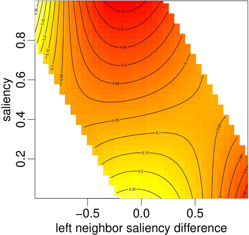
(a) Left, no chunk. ($\ast$)

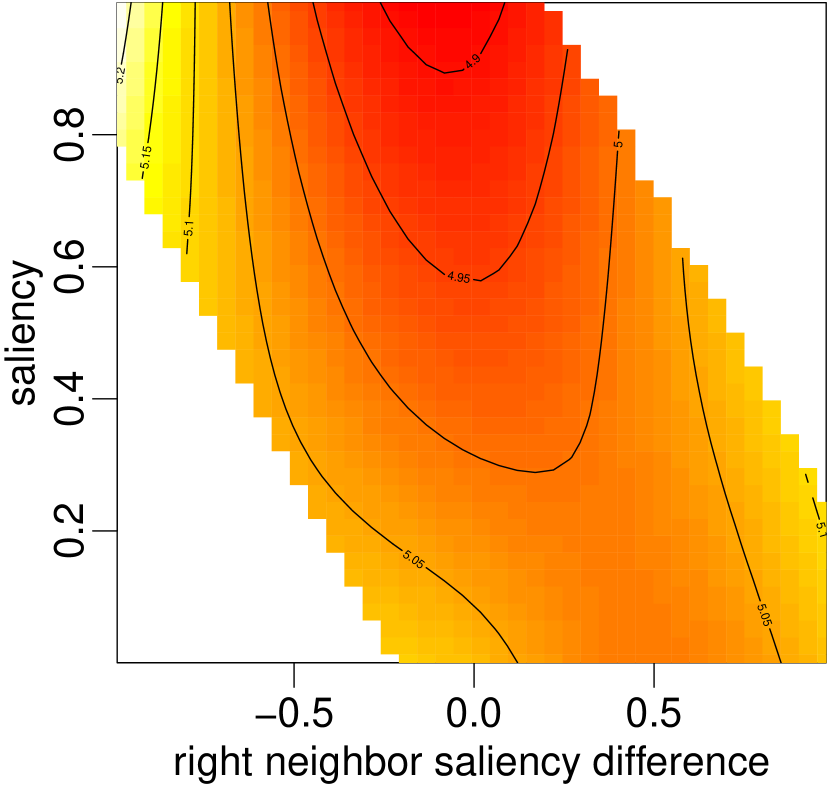
(b) Right, no chunk. ($\ast$)

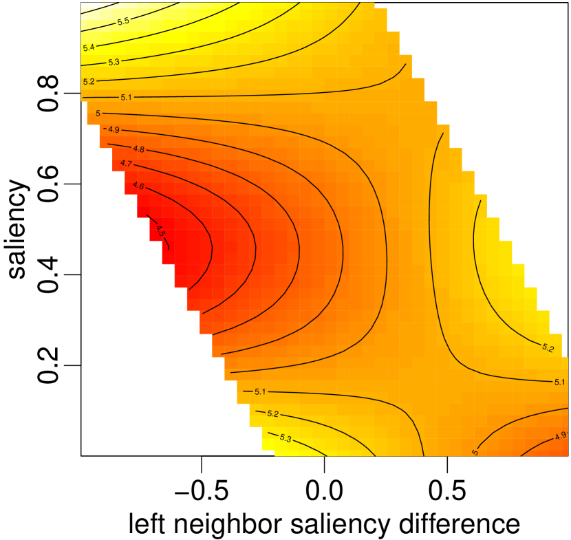
(c) Left, chunk. ($\ast$)

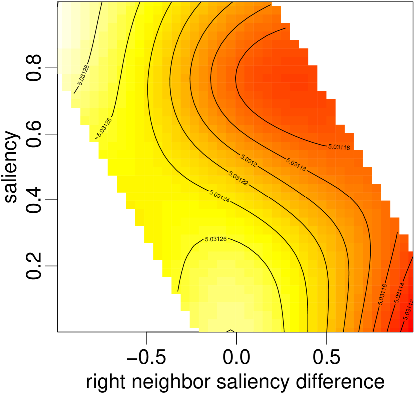
(d) Right, chunk.

Figure 3: Left and right neighbours. ($\ast$) marks statistically significant smooths. Colors are normalized per figure.

4 Neighbor Effects Analysis

In the following, we present our results for our two experiments using (a) random saliency values and (b) SHAP values.

Term	(e)df	Ref.df	F	$p$
s(saliency)	11.22	19.00	580.89	$<$0.0001
s(display index)	3.04	9.00	22.02	$<$0.0001
s(word length)	1.64	9.00	16.44	$<$0.0001
s(sentence length)	0.00	4.00	0.00	0.425
s(relative word frequency)	0.00	9.00	0.00	0.844
s(normalized saliency rank)	0.59	9.00	0.37	0.115
s(word position)	0.58	9.00	0.18	0.177
te(left diff.,saliency): no chunk	3.12	24.00	1.50	0.002
te(left diff.,saliency): chunk	2.24	24.00	0.51	0.038
te(right diff.,saliency): no chunk	2.43	24.00	0.47	0.049
te(right diff.,saliency): chunk	0.00	24.00	0.00	0.578
capitalization	2.00		3.15	0.042
dependency relation	35.00		2.92	$<$0.0001

Table 2: (Effective) degrees of freedom, reference degrees of freedom and Wald test statistics for the univariate smooth terms (top) and parametric terms (bottom) for our randomized saliency experiment.

4.1 Randomized Explanations

Regarding our additionally introduced neighbor terms, Figure 3 shows the estimates for the four described functions (left/right $\times$ chunk/no chunk). Table 2 lists all smooth and parametric terms along with Wald test results Wood (2013a, b). Appendix A includes additional results.

Asymmetric influence.

Figure 3(a) vs. Figure 3(b) and Figure 3(c) vs. Figure 3(d) reveal qualitative differences between left and right neighbor’s influences. We quantitatively confirm these differences by calculating areas of significant differences Fasiolo et al. (2020); Marra and Wood (2012). Figures 4(a) and 4(b) show the respective plots of (significant) differences and probabilities for the chunk case. Overall, we conclude that the influence from left and right word neighbors is significantly different.
Chunk influence. We investigate the difference between neighbors that are within a chunk with the rated word vs. those that are not. We find qualitative differences in Figure 3 as well as statistically significant differences (Figures 4(c) and 4(d)).
Saliency moderates neighbor difference. Figure 3 shows that the effect of a neighbor’s saliency difference (x-axis) is moderated by the rated word’s saliency (y-axis). We confirm this observation statistically (Figure 4(e)) by comparing functions at a rated word saliency of 0.25 and 0.75, using unidimensional difference plots Van Rij et al. (2015).
Combined effects. We identify two general opposing effects: assimilation and contrast.

We refer to Assimilation as situations where a word’s perceived saliency is perceived as more (or less) important based on whether its neighbor has a higher (or lower) saliency. We find assimilation effects from left neighbors that form a chunk with a moderate saliency (0.25–0.75) rated word.

We refer to Contrast as situations where a word’s perceived saliency is perceived as less (or more) important based on whether its neighbor has a higher (or lower) saliency. We find contrast effects from left and right neighbors that do not form a chunk with the rated word.

(a) Right/left difference for chunks (contour marks 0).

(b) Right/left difference (chunk) $p$ values (contour marks 0.05).

(c) Chunk/no chunk difference for left neighbor (contour marks 0).

(d) Chunk/no chunk difference (left) $p$ values (contour marks 0.05).

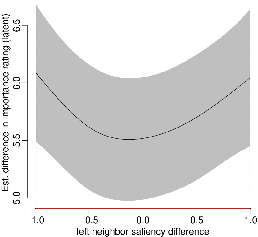
(e) Difference between rated saliency and left neighbor saliency.

Figure 4: Difference plots. Contour refers to the contour line. Red x-axis in (e) marks significant differences.

4.2 SHAP-Value Explanations

Shared results.

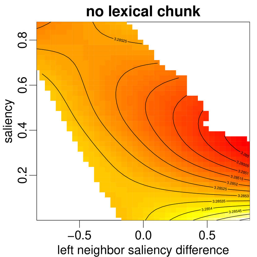
(a) Left, no chunk.

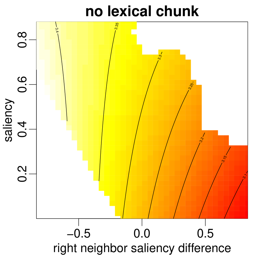
(b) Right, no chunk.

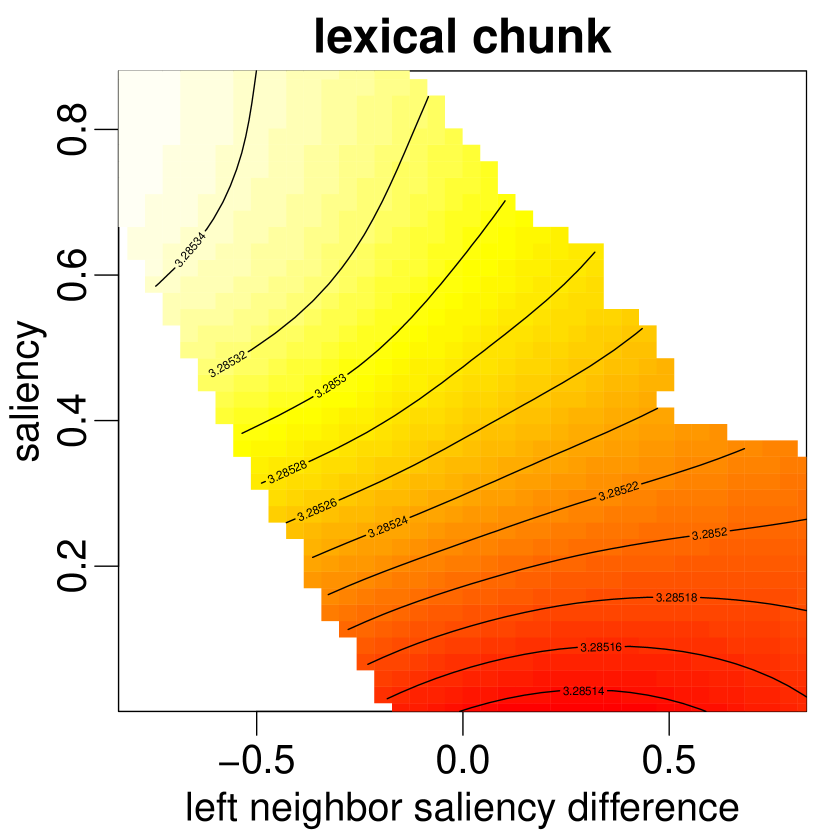
(c) Left, chunk.

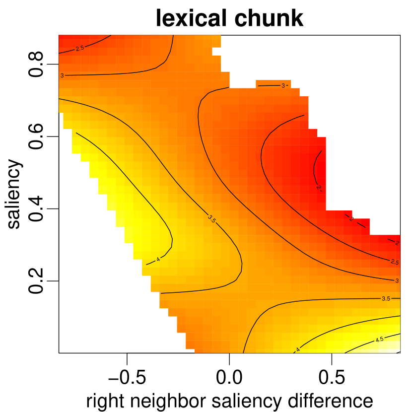
(d) Right, chunk. ($\ast$)

Figure 10: Left and right neighbours in our SHAP-value experiment. ($\ast$) marks statistically significant smooths. Colors are normalized per figure. Note that the first three plots correspond to non-significant effects and their respective color mappings covers a small value range.

Our SHAP-value experiment confirms our observation of (i) asymmetric influence of left/right neighbors (Figures 11(a) and 11(b)), (ii) chunk influence (Figures 11(c) and 11(d)), (iii) a moderating effect of saliency (Figure 11(e)), and (iv) assimilation and contrast effects (Figure 10(d)).

Variant results.

Notably, our SHAP-value results differ from our randomized saliency results with respect to the effects left/right direction. For the randomized saliency experiment, we observe assimilation effects from left neighbors within a chunk (Figure 3(c)) and contrast effects from left and right neighbors outside a chunk (Figures 3(a) and 3(b)). For our SHAP-value experiment, we observe assimilation (low rated word saliencies) and contrast effects (medium normalized rated word saliencies) from right neighbors within a chunk (Figure 10(d)). We hypothesize that this difference can be attributed to the inter-dependencies of SHAP values as indicated in Figure 12 in Appendix B.

4.3 Takeaways

Overall, we find that (a) left/right influences are not the same, (b) strong bigram relationships can invert contrasts into assimilation for left neighbors, (c) extreme saliencies can inhibit assimilation, and (d) biasing effects can be observed for randomized explanations as well as SHAP-value explanations.

5 Theoretical Grounds in Psychology

The assimilation effect is, of course, intuitive—it simply mean that neighbors’ importance “leaks” from neighbor to the rated word for strong bigram relationships. But is there precedence for the observed assimilation and contrast effects in the literature? How do they relate to each other?

Psychology investigates how a prime (e.g., being exposed to a specific word) influences human judgement, as part of two categories: assimilation (the rating is “pulled” towards the prime) and contrast (the rating is “pushed” away from the prime) effects (i.a., Bless and Burger, 2016).

Förster et al. (2008) demonstrate how global processing (e.g. looking at the overall structure) vs. local processing (e.g., looking at the details of a structure) leads to assimilation vs. contrast. We argue that some of our observations can be explained with their model: Multi-word phrase neighbors may induce global processing that leads to assimilation (for example, in the randomized explanation experiments, left neighbors) while other neighbors (in the randomized explanation experiments, right neighbors and unrelated left neighbors) induce local processing that leads to contrast. Future work may investigate the properties that induce global processing in specific contexts.

6 Conclusions

We conduct a user study in a setting of laypeople observing common word-importance explanations, as color-coded importance, in the English Wikipedia domain. In this setting, we find that when the explainee understands the attributed importance of a word, the importance of other words can influence their understanding in unintended ways.

Common wisdom posits that when communicating the importance of a component in a feature-attribution explanation, the explainee will understand this importance as it is shown. We find that this is not the case: The explainee’s contextualized understanding of the input portion—for us, a word as a part of a phrase—may influence their understanding of the explanation.

Limitations

The observed effects in this work, in principle, can only be applied to the setting of our user study (English text, English-speaking crowd-workers, color-coded word-level saliency, and so on, as described in the paper). Therefore this study serves only as a proof of existence, for a reasonably plausible and common setting in NLP research, that laypeople can be influenced by context outside of the attributed part of the input when comprehending a feature-attribution explanation. Action taken on design and implementation of explanation technology for NLP systems in another setting, or other systems of similar nature, should either investigate the generalization of effects to the setting in practice (towards which we aim to release our full reproduction code), or take conservative action in anticipation that the effects will generalize without compromising the possibility that they will not.

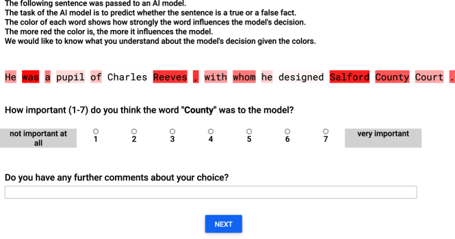
Figure 5: Screenshot of the rating interface.

Appendix A User Study Details

This section provides details on our user study setup.

A.1 Interface

Figure 5 shows a screenshot of our rating interface. Figure 6 shows a screenshot of an attention check.

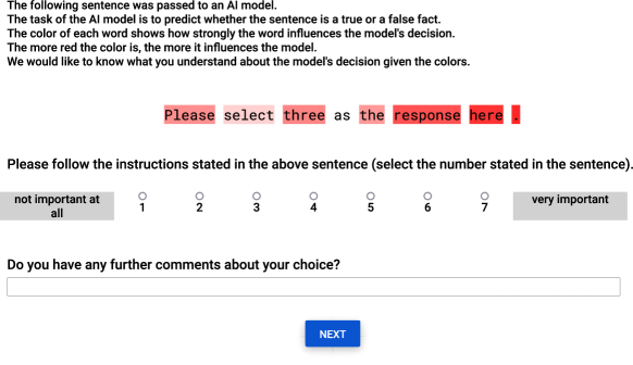
Figure 6: Screenshot of the rating interface for an attention check.

A.2 Attention Checks

We include three attention checks per participants which we randomly place within the last two thirds of the study following Schuff et al. (2022).

A.3 Participants

In total, we recruit 76 crowd workers from English-speaking countries via Amazon Mechanical Turk for our randomized explanation study and 36 crowd workers for our SHAP-value explanation study. We require workers to have at least 5,000 approved HITs and 95% approval rate. Raters are screened with three hidden attention checks that they must answer correctly to be included (but are paid fully regardless). From the 76 workers, 64 workers passed the screening, i.e., we excluded 15.8% of responses on a participant level. From the 36 workers, all workers passed the screening. On average, participants were compensated with an hourly wage of US$8.95. We do not collect any personally-identifiable data from participants.

Appendix B Statistical Model Details

In this section, we give a brief general introduction to statistical model we used (i.e., GAMM) and provide additional results of our analysis.

B.1 Introduction to GAMM Models

We refer to the very brief introduction to GAMMs in Schuff et al. (2022) (appendix). Very briefly, an ordinal GAMM can be described as a generalized additive model that additionally accounts for random effects and models ordinal ratings via a continuous latent variable that is separated into the ordinal categories via estimated threshold values. For further details, Divjak and Baayen (2017) provide a practical introduction to ordinal GAMs in a linguistic context and Wood (2017) offers a detailed textbook on GAM(M)s including implementation and analysis details.

Examples

The Emerging Pathogens Institute is an interdisciplinary research institution associated with the University of Florida.

Luca Emanuel Meisl (born 4 March 1999) is an Austrian footballer currently playing for FC Liefering.

The black-throated toucanet (Aulacorhynchus atrogularis) is a near-passerine bird found in central Ecuador to western Bolivia.

Christopher Robert Coste (born February 4, 1973) is an author and former Major League Baseball catcher.

WGTA surrendered its license to the Federal Communications Commission (FCC) on November 3, 2014.

Table 3: Examples of Wikipedia sentences used in our study.

B.2 Model Details in Our Analysis

We control for all main effects (word length, sentence length etc.) as well as all random effects used by Schuff et al. (2022). We exclude the pairwise interactions due to model instability when including the interactions.

We additionally include four new novel bivariate smooth terms. Each of these terms models a tensor product of saliency (i.e. the rated word’s color intensity) and the neighboring (left or right) word’s saliency difference to the rated word. For each side (left and right), we model the smooths for neighbors that (i) are within a lexical chunk to the rated word and (ii) are not. Figure 3 shows the estimated four (bivariate) functions.

B.3 Data Preprocessing

Following Schuff et al. (2022), we exclude ratings with a completion time of less than a minute (implausibly fast completion) and exclude words with a length over 20 characters. We effectively exclude 1.8% of ratings.

In order to analyze left as well as right neighbors, we additionally have to ensure that we only include ratings for which both—left and right— neighbors exist. Therefore, we additionally exclude rating for which the leftmost or rightmost word in the sentence was rated. This excludes 11.7% of ratings. In total, we thus use 9489 ratings to fit our model.

B.4 Chunk Measures

We explore and combine two approaches of identifying multi-word phrases (or “chunks)”.

Syntactic measures (constituents).

We first apply binary chunk measures based on the sentences’ parse trees. We use Stanza Qi et al. (2020) (version 1.4.2) to generate parse tree for each sentence. We assess whether the rated word and its neighbor (left/right) share a constituent at the lowest possible level. Concretely, we (a) start at the rated word and move up one level in the parse tree and (b) start at the neighboring word and move up one level in the parse tree. If we now arrived at the same node in the parse tree, we the rated word and its neighbor share a first-order constituent. If we arrived at different nodes, they do not. Restricting the type of first-level shared constituents to noun phrases yields a further category. We provide respective examples for shared first-level constituents and the respective noun phrase constituents extracted from our data in Table 4 (upper part).

Statistical measures (cooccurrence scores).

We additionally explore numeric association measures and calculate all available bigram collocation measures available in NLTK’s BigramAssocMeasures module. The calculation is based on the 7 million Wikipedia-2018 sentences in Wikipedia Sentences (Footnote 5). A description of each metric as well as top-scored examples on our data is provided in Table 4 (lower part). We separate examples into examples that form a constituent vs. do not form a constituent to highlight the necessity to apply a constituent filter in order to get meaningful categorization into chunks vs. no chunks.

Measure	Constituent Examples	No Constituent Examples	Description
First-order constituent	highly developed, more than, such as, DVD combo, 4 million	—	Smallest multi-word constituent sub-trees in the constituency tree.
Noun phrase	Tokyo Marathon, ski racer, the UK, a retired, the city	—	Multi-word first-order noun phrase in the constituency tree.
Mutual information	as well, more than, ice hockey, United Kingdom, a species	is a, of the, in the, is an, it was	Bigram mutual information variant (per NLTK implementation).
Frequency	the United, the family, a species, an American, such as	of the, in the, is a, to the, on the	Raw, unnormalized frequency.
Poisson Stirling	an American, such as, a species, as well, the family	is a, of the, in the, is an, it was, has been	Poisson Stirling bigram score.
Jaccard	Massar Egbari, ice hockey, Air Force, more than, Udo Dirkschneider	teachers/students teaching/studying, is a, has been, it was, of the	Bigram Jaccard index.
$\upvarphi^{2}$	Massar Egbari, ice hockey, Udo Dirkschneider, Air Force, New Zealand	teachers/students teaching/studying, is a, has been, footballer who, is an	Square of the Pearson correlation coefficient.

Table 4: The list of phrase measures we tested for. Examples for numeric measures are chosen based on highest cooccurrence scores whereas the (boolean) noun phrase and constituent examples are chosen arbitrarily. For the numeric measures, we provide examples that (a) form a constituent with their neighbor and (b) do not. The examples underline the necessity to combine numeric scores with a constituent filter.

B.5 Detailed Results

As described in Section 4, we observe different influences of left/right neighbors, chunk/no chunk neighbors as well as rated word saliency levels in our randomized explanation experiment.

Left vs. right neighbors.

Figure 7 shows difference plots (and respective p values) between left and right neighbors for chunk neighbors (Figures 7(a) and 7(b)) and no chunk neighbors (Figures 7(c) and 7(d)).

Chunk vs. no chunk.

Respectively, Figure 8 shows difference plots (and respective p values) between chunk and no chunk neighbors for left neighbors (Figures 8(a) and 8(b)) and right neighbors (Figures 8(c) and 8(d)).

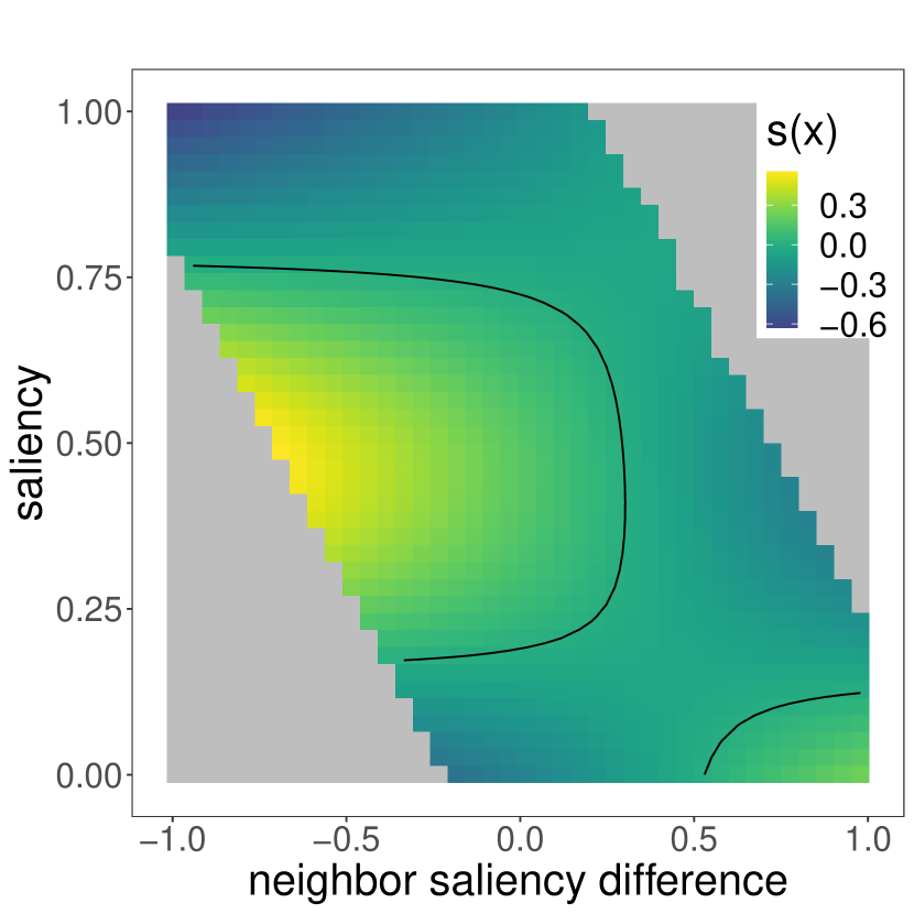
(a) Difference between right - left (chunk). The contour line marks zero.

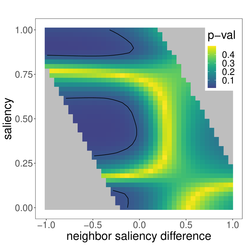
(b) Difference (chunk) $p$ values. The contour line marks 0.05.

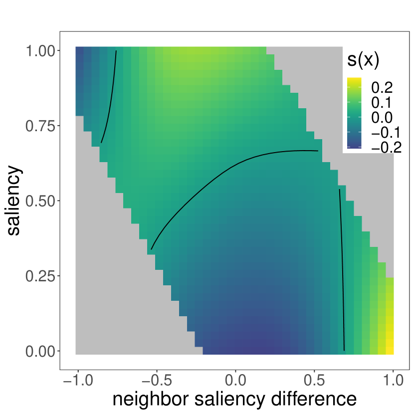
(c) Difference between right - left (no chunk). The contour line marks zero.

(d) Difference (no chunk) $p$ values. The contour line marks 0.05.

Figure 7: Differences and $p$ values for (no) lexical chunk neighbors for our randomized explanation experiment.

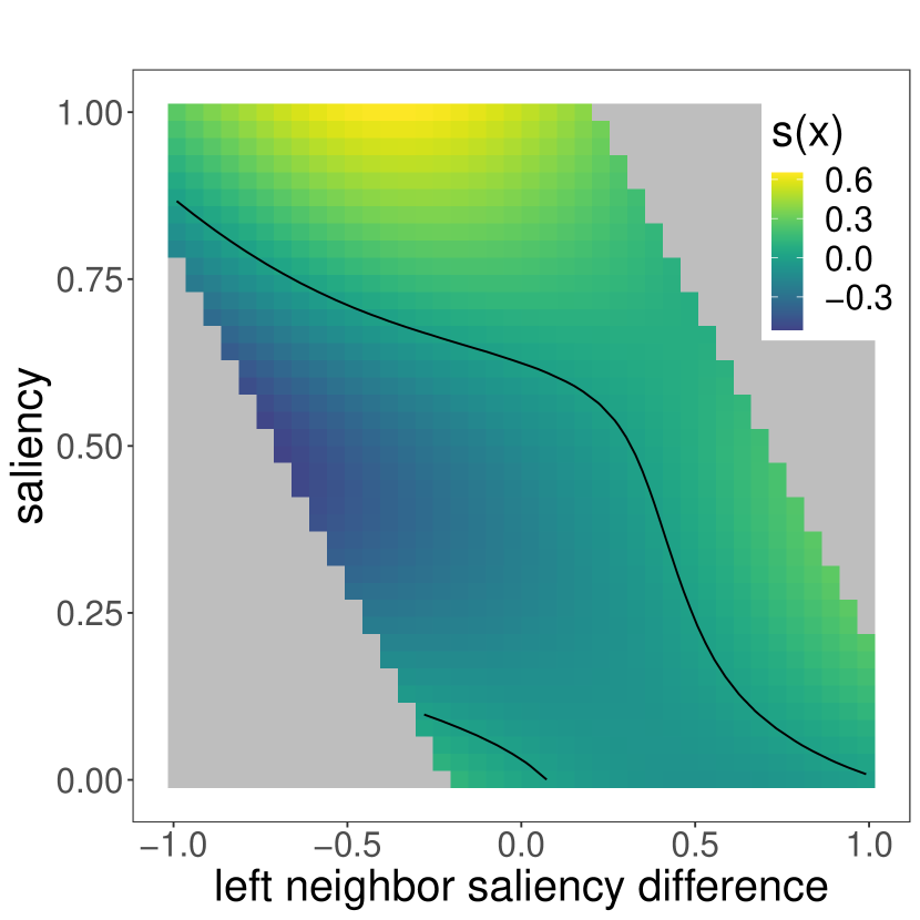
(a) Difference between (left neighbors) chunk - no chunk. The contour line marks zero.

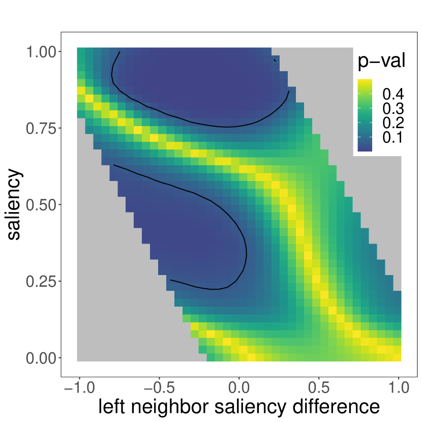
(b) Difference (left neighbors) $p$ values. The contour line marks 0.05.

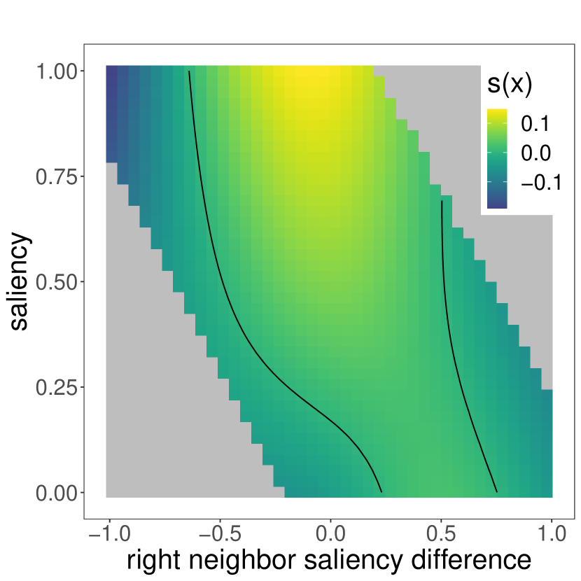
(c) Difference between (right neighbors) chunk - no chunk. The contour line marks zero.

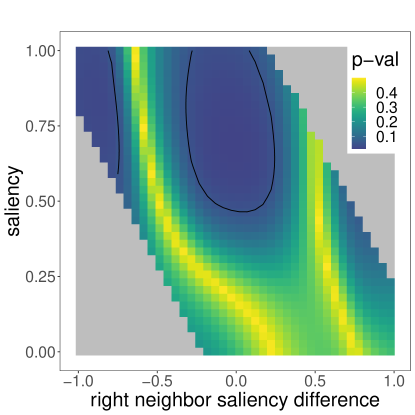
(d) Difference (right neighbors) $p$ values. The contour line marks 0.05.

Figure 8: Differences and $p$ values for left and right neighbors for our randomized explanation experiment.

Differences across saliency levels.

Figure 9 shows that the effects of saliency difference are significantly different between different levels of the rated word’s saliency (0.25 and 0.75) for left neighbors (Figure 9(a)) as well as right neighbors (Figure 9(b)).

(a) Left.

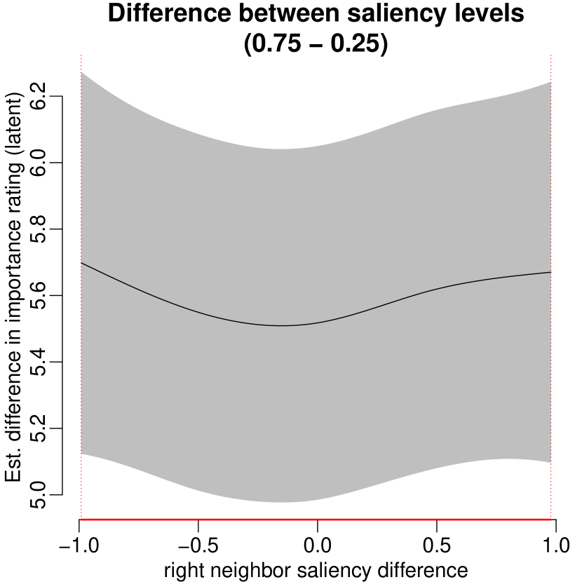
(b) Right.

Figure 9: Difference plots between the influence of saliency differences between exemplary high (0.75) and low (0.25) rated word saliency levels. Red x-axis areas indicate significant differences.

We report the detailed Wald test statistics for our randomized explanation experiment in Table 5.

B.6 SHAP-value Results

We additionally report details regarding our SHAP-value experiment results. Figure 11 displays left/right, chunk/no chunk, and rated word saliency level difference plots. We report the detailed Wald test statistics for our SHAP-value explanation experiment in Table 6. Figure 12 illustrates how the distribution of saliency scores is uniforlmy random for our randomized explanations in contrast to the distributions of SHAP values.

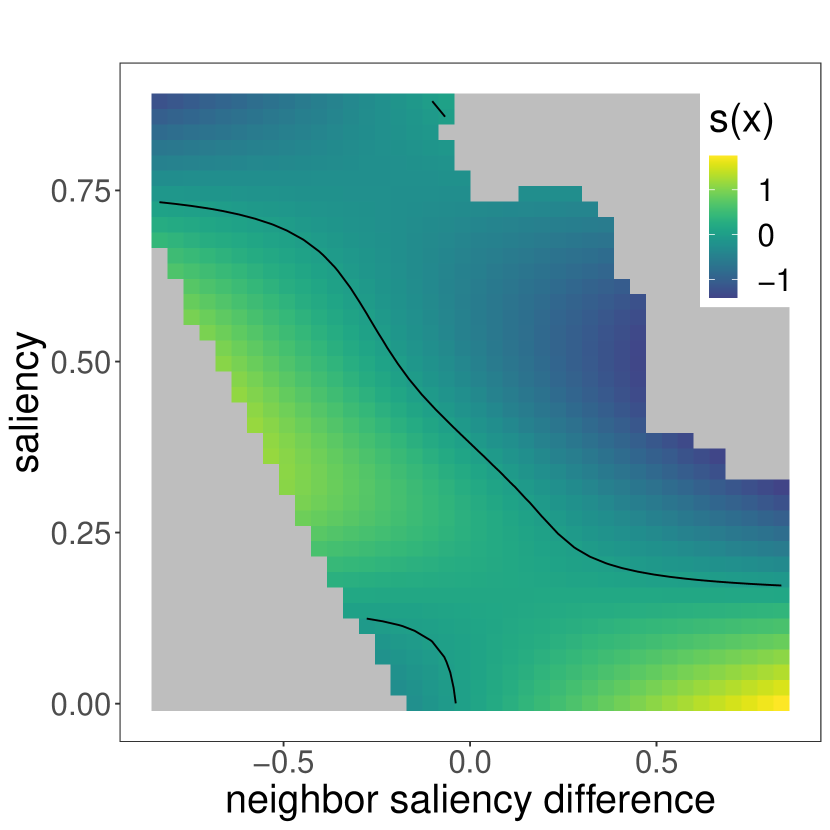
(a) Right/left difference for chunks (contour marks 0).

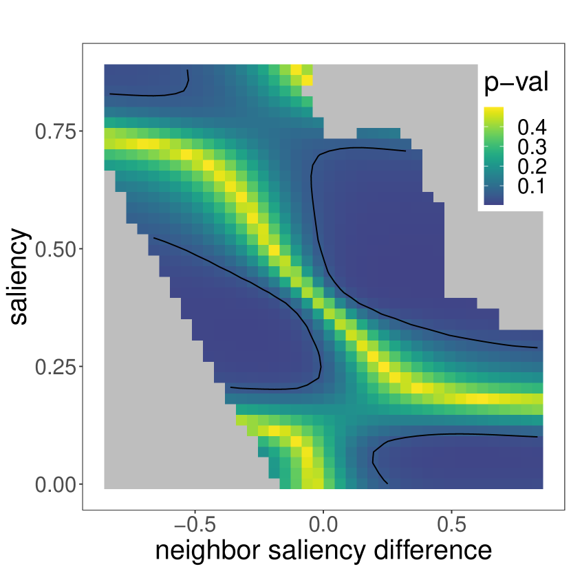
(b) Right/left difference (chunk) $p$ values (contour marks 0.05).

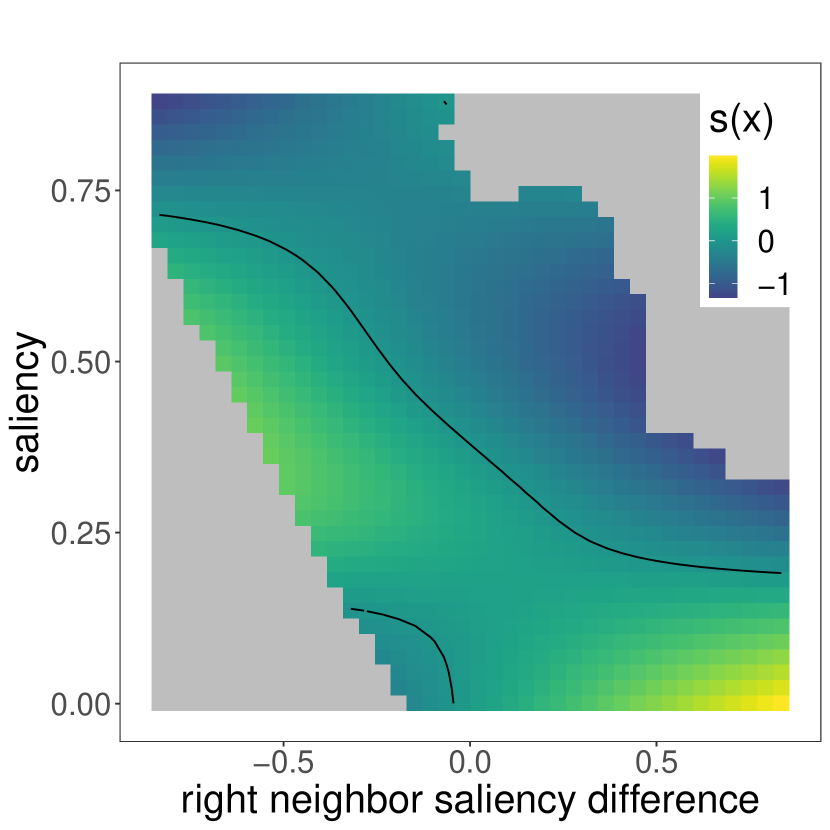
(c) Chunk/no chunk difference for right neighbor (contour marks 0).

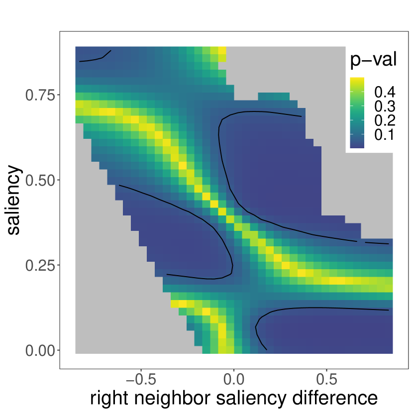
(d) Chunk/no chunk difference (right) $p$ values (contour marks 0.05).

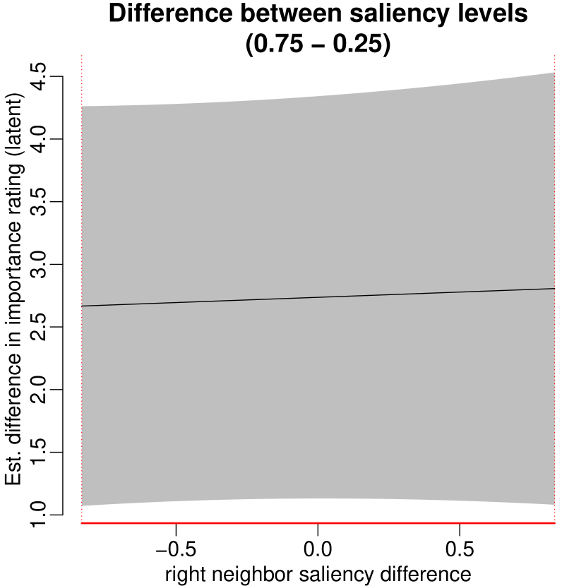
(e) Difference between rated saliency and right neighbor saliency.

Figure 11: Difference plots of our SHAP-value experiment results. Contour refers to the contour line. Red x-axis in (e) marks significant differences.

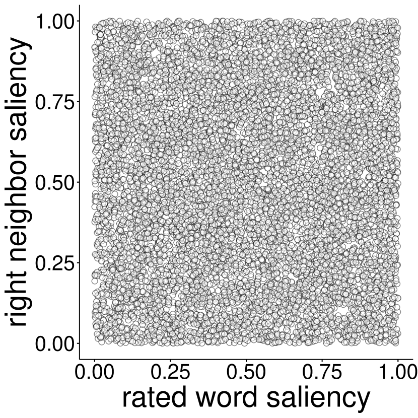
(a) Randomized saliency.

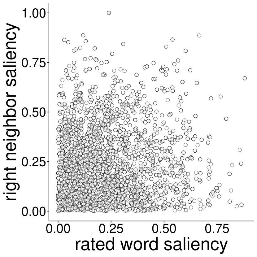
(b) SHAP-value saliency.

Figure 12: Comparison of the distributions of rated word saliency and right neighbor saliency across our randomized explanations (left) and our SHAP-value experiments (right).

B.7 Reproduction of Schuff et al. (2022)

We confirm previous results from Schuff et al. (2022) and find significant effects of word length, display index, capitalization, and dependency relation. We report detailed statistics of our randomized saliency experiment in Table 5 and our SHAP experiment in Table 6.

Term	(e)df	Ref.df	F	$p$
s(saliency)	11.22	19.00	580.89	$<$0.0001
s(display index)	3.04	9.00	22.02	$<$0.0001
s(word length)	1.64	9.00	16.44	$<$0.0001
s(sentence length)	0.00	4.00	0.00	0.425
s(relative word frequency)	0.00	9.00	0.00	0.844
s(normalized saliency rank)	0.59	9.00	0.37	0.115
s(word position)	0.58	9.00	0.18	0.177
te(left diff.,saliency): no chunk	3.12	24.00	1.50	0.002
te(left diff.,saliency): chunk	2.24	24.00	0.51	0.038
te(right diff.,saliency): no chunk	2.43	24.00	0.47	0.049
te(right diff.,saliency): chunk	0.00	24.00	0.00	0.578
s(sentence ID)	0.00	149.00	0.00	0.616
s(saliency,sentence ID)	16.13	150.00	0.14	0.191
s(worker ID)	62.19	63.00	30911.89	$<$0.0001
s(saliency,worker ID)	62.11	64.00	16760.88	$<$0.0001
capitalization	2.00		3.15	0.042
dependency relation	35.00		2.92	$<$0.0001

Table 5: Random saliency experiment results details. (Effective) degrees of freedom, reference degrees of freedom and Wald test statistics for the univariate smooth terms (top), random effects terms (middle) and parametric fixed terms (bottom) using $t=87.5\%$ and $\upvarphi^{2}$ measure.

Term	(e)df	Ref.df	F	$p$
s(saliency)	6.71	19.00	18.85	$<$0.0001
s(display index)	1.88	9.00	6.45	$<$0.0001
s(word length)	2.04	9.00	4.43	$<$0.0001
s(sentence length)	0.00	4.00	0.00	0.98
s(relative word frequency)	0.00	9.00	0.00	0.64
s(normalized saliency rank)	0.89	9.00	1.99	0.002
s(word position)	0.42	9.00	0.12	0.19
te(left diff.,saliency): no chunk	0.00	24.00	0.00	0.37
te(left diff.,saliency): chunk	0.00	24.00	0.00	0.49
te(right diff.,saliency): no chunk	0.99	24.00	0.20	0.06
te(right diff.,saliency): chunk	3.24	24.00	1.09	0.01
s(sentence ID)	0.00	149.00	0.00	0.52
s(saliency,sentence ID)	11.31	150.00	0.10	0.14
s(worker ID)	34.77	35.00	14185.28	$<$0.0001
s(saliency,worker ID)	62.11	64.00	16760.88	$<$0.0001
capitalization	2.00	0.35	0.71
dependency relation	34.59	36.00	8468.22	$<$0.0001

Table 6: SHAP experiment results details. (Effective) degrees of freedom, reference degrees of freedom and Wald test statistics for the univariate smooth terms (top), random effects terms (middle) and parametric fixed terms (bottom) using $t=87.5\%$ and $\upvarphi^{2}$ measure.

Appendix C Robustness to Evaluation Parameters.

To ensure our results are not an artifact of the particular combination of threshold and cooccurrence measure, we investigate how our results change if we (i) vary the threshold within $\{0.5,0.75,0.875\}$ and (ii) vary the cooccurence measure within {Jaccard, MI-like, $\upvarphi^{2}$, Poisson-Stirling}. We find significant interactions and observe similar interaction patterns as well as areas of significant differences (left/right, chunk/no chink as well as saliency levels) across all settings. We provide a representative selection of plots in Figures 13, 14, 15, 16, 17 and 18. Additionally, Tables 7 and 8 demonstrate that changing the threshold or cooccurrence measure leads to model statistics that are largely consistent with the results reported in Table 5. We choose the $\upvarphi^{2}$ and a 87.5% threshold as no other model reaches a higher deviance explained and a comparison of randomly-sampled chunk/no chunk examples across measures and thresholds yields the best results for this setting.

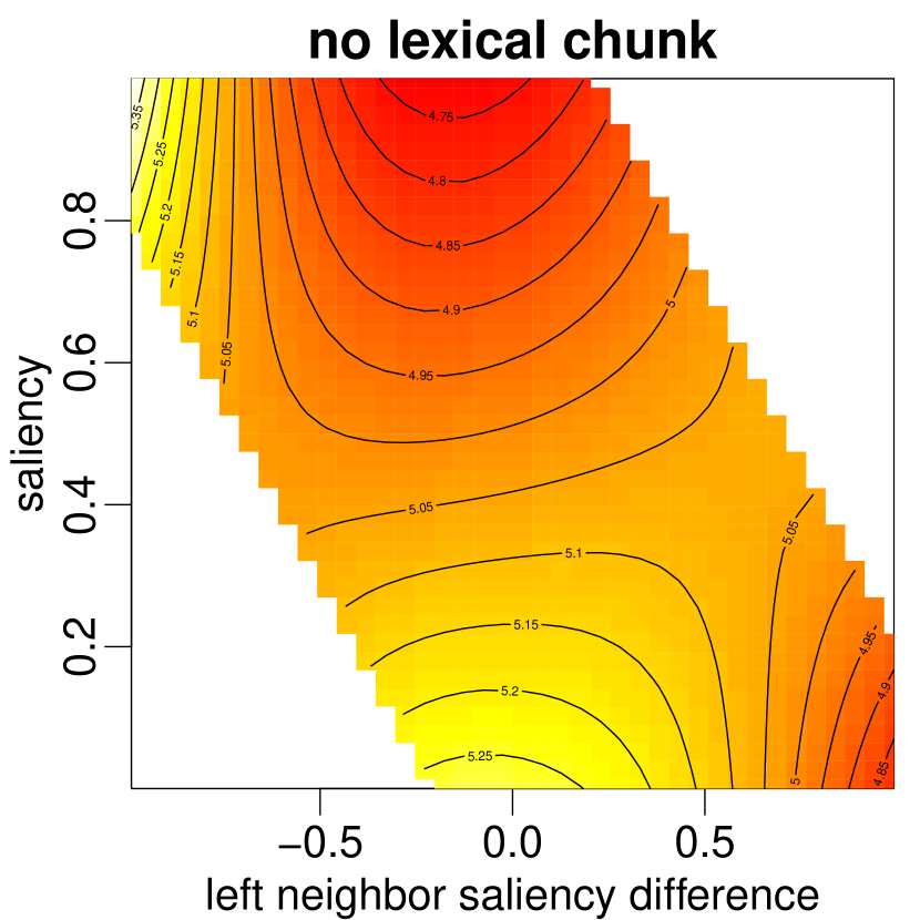
(a) $\upvarphi^{2}$.

(b) Jaccard.

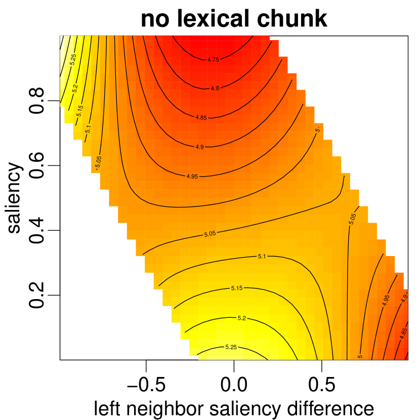
(c) MI-like.

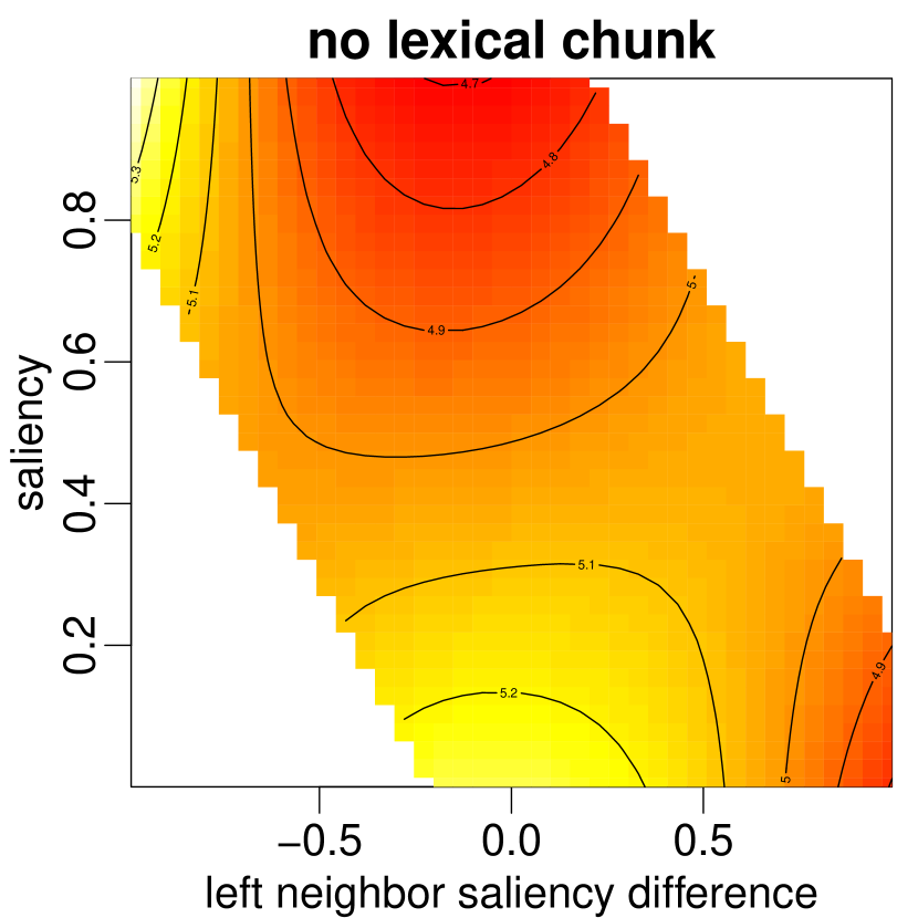
(d) Poisson-Stirling.

Figure 13: Tensor product interactions for left saliency difference in the outside chunk setting across different choices of cooccurrence measures for our randomized explanation experiment. We find similar patterns across all settings. $t=87.5$ is consistent for all plots.

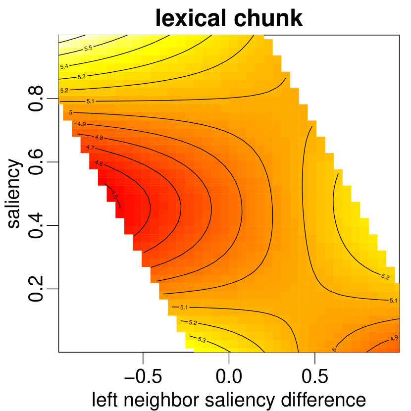
(a) $\upvarphi^{2}$.

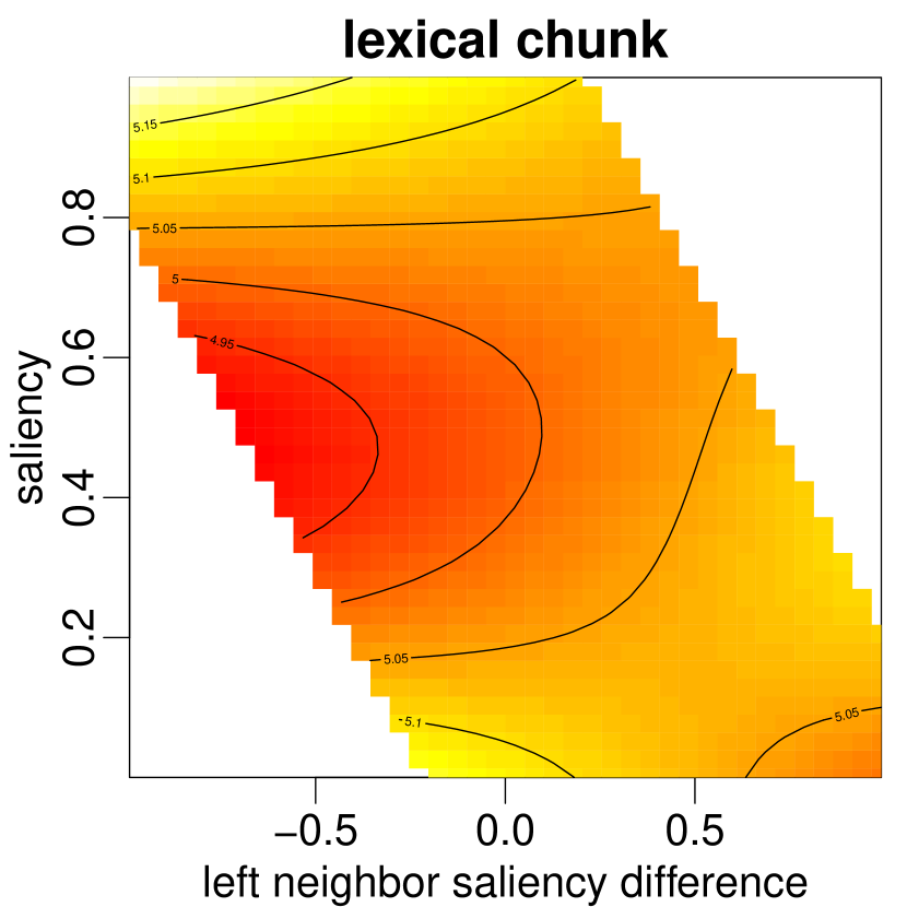
(b) Jaccard.

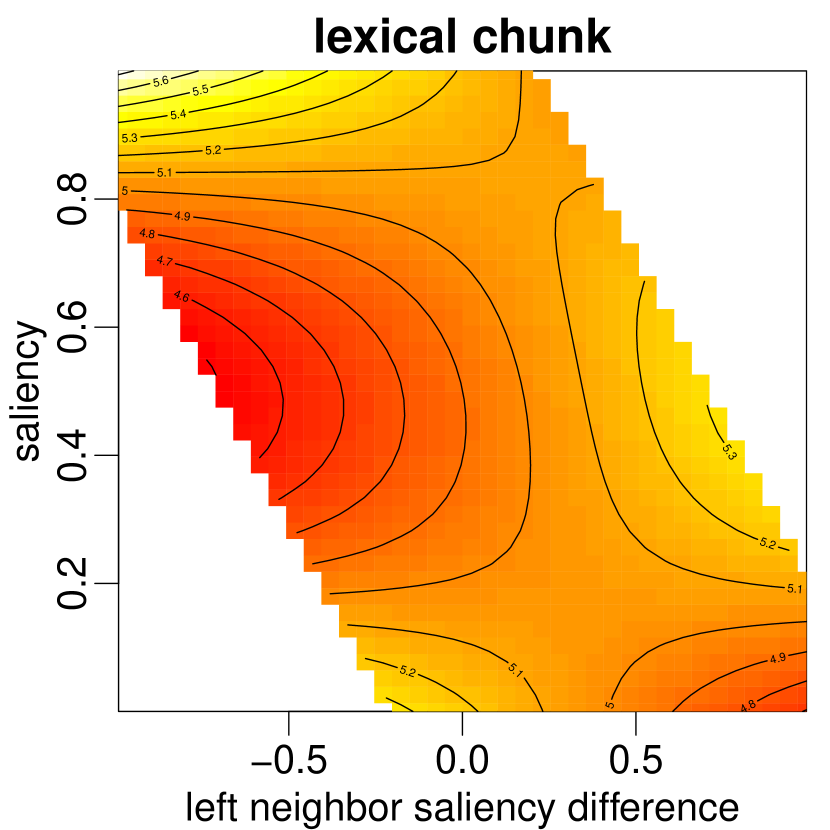
(c) MI-like.

(d) Poisson-Stirling.

Figure 14: Tensor product interactions for left saliency difference in the within chunk setting across different choices of cooccurrence measures for our randomized explanation experiment. We find similar patterns across all settings. $t=87.5$ is consistent for all plots.

(a) $\upvarphi^{2}$.

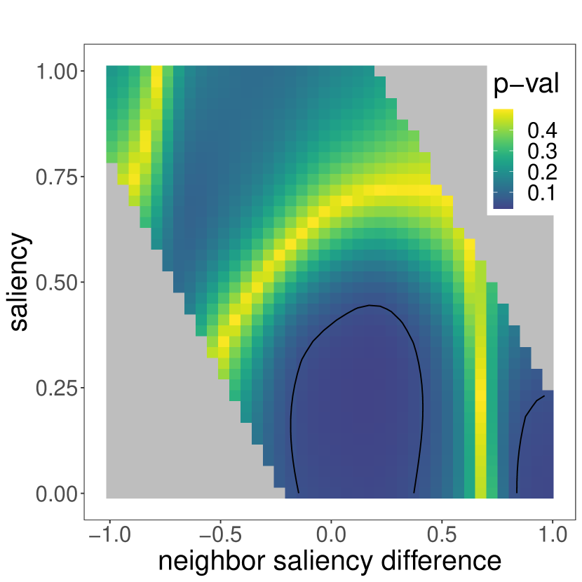
(b) Jaccard.

(c) MI-like.

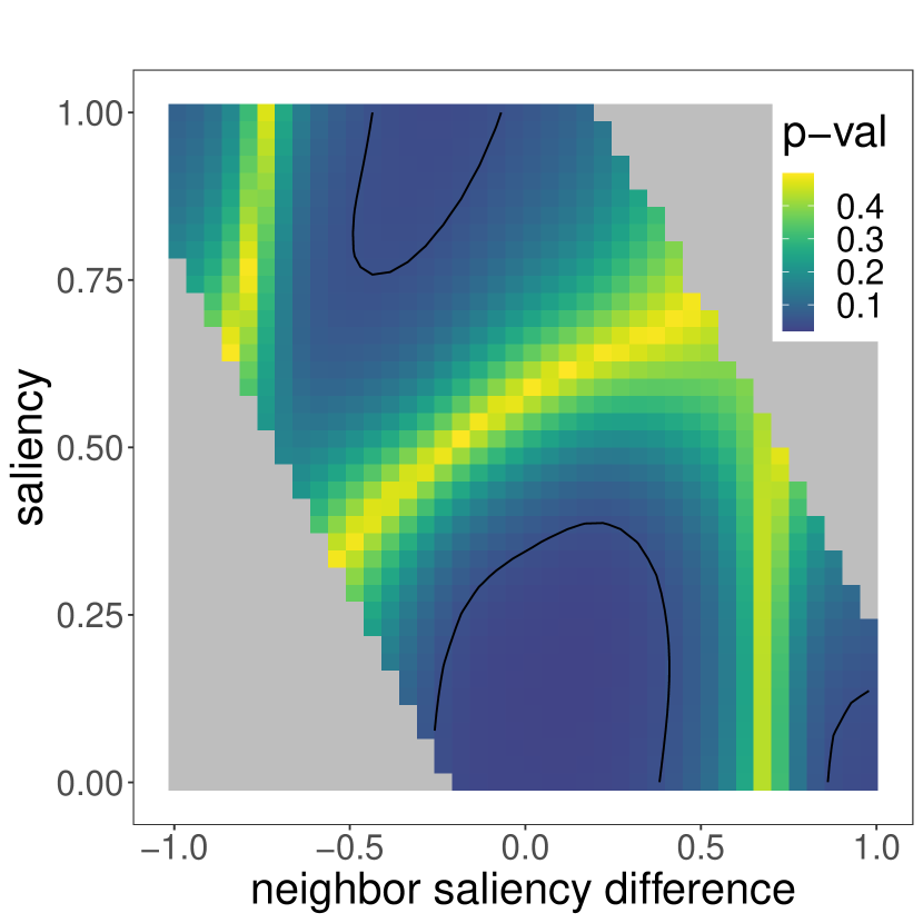
(d) Poisson-Stirling.

Figure 15: $p$ values for between right - left for no lexical chunk neighbors across different choices of cooccurrence measures for our randomized explanation experiment. We find similar patterns across all settings. $t=87.5$ is consistent for all plots.

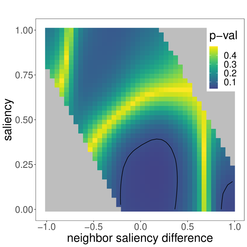
(a) $t=87.5\%$

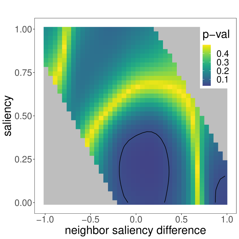
(b) $t=75\%$

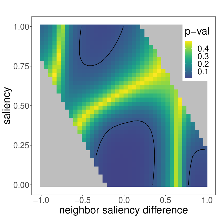
(c) $t=50\%$

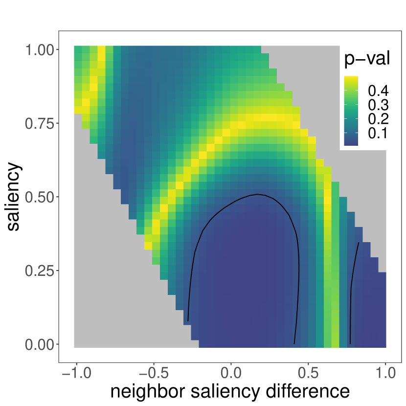
(d) $t=25\%$

Figure 16: $p$ values for differences between right - left for no lexical chunk neighbors across different choices of thresholds for our randomized explanation experiment. We find similar patterns across all settings. The $\upvarphi^{2}$ measure is used across all plots.

(a) $t=87.5\%$

(b) $t=75\%$

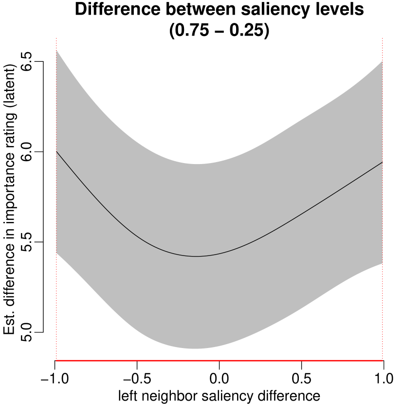
(c) $t=50\%$

(d) $t=25\%$

Figure 17: Difference plots between the influence of left saliency differences between exemplary high (0.75) and low (0.25) rated word saliency levels across different choices of thresholds for our randomized explanation experiment. We find similar patterns across all settings. The $\upvarphi^{2}$ measure is used across all plots.

(a) $\upvarphi^{2}$.

(b) Jaccard.

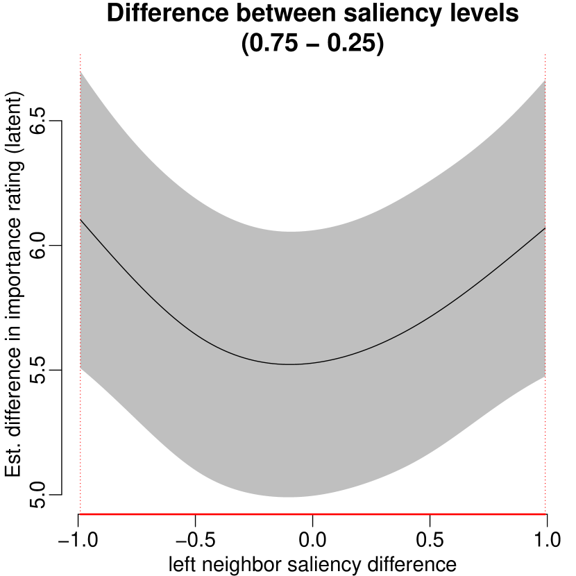
(c) MI-like.

(d) Poisson-Stirling.

Figure 18: Difference plots between the influence of left saliency differences between exemplary high (0.75) and low (0.25) rated word saliency levels across across different choices of cooccurrence measures for our randomized explanation experiment. We find similar patterns across all settings. $t=87.5$ is consistent for all plots.

Term	(e)df	Ref.df	F	$p$
s(saliency)	11.23	19.00	547.16	$<$ 0.0001
s(display_index)	3.10	9.00	20.93	$<$ 0.0001
s(word_length)	1.61	9.00	16.47	$<$ 0.0001
s(sentence_length)	0.00	4.00	0.00	0.436
s(relative_word_frequency)	0.00	9.00	0.00	0.814
s(normalized_saliency_rank)	0.58	9.00	0.36	0.120
s(word_position)	0.59	9.00	0.18	0.173
te(left diff.,saliency): no chunk	2.90	24.00	1.21	0.003
te(left diff.,saliency): chunk	3.34	24.00	0.92	0.015
te(right diff.,saliency): no chunk	2.50	24.00	0.67	0.021
te(right diff.,saliency): chunk	0.00	24.00	0.00	0.836
s(sentence_id)	0.00	149.00	0.00	0.601
s(saliency,sentence_id)	17.35	150.00	0.15	0.178
s(worker_id)	62.19	63.00	30421.05	$<$ 0.0001
s(saliency,worker_id)	62.11	64.00	17591.01	$<$ 0.0001
capitalization	2.00		3.01	0.049
dependency_relation	35.00		2.93	$<$ 0.0001

Table 7: (Effective) degrees of freedom, reference degrees of freedom and Wald test statistics for the univariate smooth terms (top), random effects terms (middle) and parametric fixed terms (bottom) using $t=25\%$ and $\upvarphi^{2}$ measure for our randomized explanation experiment.

Term	(e)df	Ref.df	F	$p$
s(saliency)	11.21	19.00	584.57	$<$ 0.0001
s(display_index)	3.04	9.00	21.63	$<$ 0.0001
s(word_length)	1.63	9.00	16.66	$<$ 0.0001
s(sentence_length)	0.00	4.00	0.00	0.407
s(relative_word_frequency)	0.00	9.00	0.00	0.813
s(normalized_saliency_rank)	0.56	9.00	0.32	0.130
s(word_position)	0.65	9.00	0.22	0.159
te(left diff.,saliency): no chunk	3.10	24.00	1.57	0.0010
te(left diff.,saliency): chunk	1.79	24.00	0.34	0.082
te(right diff.,saliency): no chunk	2.37	24.00	0.47	0.048
te(right diff.,saliency): chunk	0.64	24.00	0.05	0.249
s(sentence ID)	0.00	149.00	0.00	0.638
s(saliency,sentence ID)	17.14	150.00	0.15	0.164
s(worker ID)	62.19	63.00	30521.95	$<$ 0.0001
s(saliency,worker ID)	62.11	64.00	16749.25	$<$ 0.0001
capitalization	2.00		3.23	0.039
dependency relation	35.00		2.94	$<$ 0.0001

Table 8: (Effective) degrees of freedom, reference degrees of freedom and Wald test statistics for the univariate smooth terms (top), random effects terms (middle) and parametric fixed terms (bottom) using $t=87.5\%$ and MI-like measure for our randomized explanation experiment.

References

- Arora et al. (2021) Siddhant Arora, Danish Pruthi, Norman M. Sadeh, William W. Cohen, Zachary C. Lipton, and Graham Neubig. 2021. Explain, edit, and understand: Rethinking user study design for evaluating model explanations. CoRR, abs/2112.09669.
- Arras et al. (2017) Leila Arras, Franziska Horn, Grégoire Montavon, Klaus-Robert Müller, and Wojciech Samek. 2017. " What is relevant in a text document?": An interpretable machine learning approach. PloS one, 12(8):e0181142. Publisher: Public Library of Science San Francisco, CA USA.
- Bless and Burger (2016) Herbert Bless and Axel M Burger. 2016. Assimilation and contrast in social priming. Current Opinion in Psychology, 12:26–31. Social priming.
- Burkart and Huber (2021) Nadia Burkart and Marco F. Huber. 2021. A survey on the explainability of supervised machine learning. J. Artif. Intell. Res., 70:245–317.
- Carvalho et al. (2019) Diogo V. Carvalho, Eduardo M. Pereira, and Jaime S. Cardoso. 2019. Machine learning interpretability: A survey on methods and metrics. Electronics, 8(8):832.
- Chomsky (1957) Noam Chomsky. 1957. Syntactic Structures. De Gruyter Mouton, Berlin, Boston.
- Danilevsky et al. (2020) Marina Danilevsky, Kun Qian, Ranit Aharonov, Yannis Katsis, Ban Kawas, and Prithviraj Sen. 2020. A survey of the state of explainable AI for natural language processing. In Proceedings of the 1st Conference of the Asia-Pacific Chapter of the Association for Computational Linguistics and the 10th International Joint Conference on Natural Language Processing, AACL/IJCNLP 2020, Suzhou, China, December 4-7, 2020, pages 447–459. Association for Computational Linguistics.
- Dinu et al. (2020) Jonathan Dinu, Jeffrey P. Bigham, and J. Zico Kolter. 2020. Challenging common interpretability assumptions in feature attribution explanations. CoRR, abs/2012.02748. ArXiv: 2012.02748.
- Divjak and Baayen (2017) Dagmar Divjak and Harald Baayen. 2017. Ordinal GAMMs: a new window on human ratings. In Each venture, a new beginning: Studies in Honor of Laura A. Janda, pages 39–56. Slavica Publishers.
- Ehsan et al. (2021) Upol Ehsan, Samir Passi, Q. Vera Liao, Larry Chan, I-Hsiang Lee, Michael J. Muller, and Mark O. Riedl. 2021. The who in explainable AI: how AI background shapes perceptions of AI explanations. CoRR, abs/2107.13509.
- Fasiolo et al. (2020) Matteo Fasiolo, Raphaël Nedellec, Yannig Goude, and Simon N Wood. 2020. Scalable visualization methods for modern generalized additive models. Journal of computational and Graphical Statistics, 29(1):78–86.
- Fel et al. (2021) Thomas Fel, Rémi Cadène, Mathieu Chalvidal, Matthieu Cord, David Vigouroux, and Thomas Serre. 2021. Look at the variance! efficient black-box explanations with sobol-based sensitivity analysis. In Advances in Neural Information Processing Systems 34: Annual Conference on Neural Information Processing Systems 2021, NeurIPS 2021, December 6-14, 2021, virtual, pages 26005–26014.
- Förster et al. (2008) Jens Förster, Nira Liberman, and Stefanie Kuschel. 2008. The effect of global versus local processing styles on assimilation versus contrast in social judgment. Journal of personality and social psychology, 94(4):579.
- Frantzi et al. (2000) Katerina T. Frantzi, Sophia Ananiadou, and Hideki Mima. 2000. Automatic recognition of multi-word terms:. the c-value/nc-value method. International Journal on Digital Libraries, 3:115–130.
- Gonzalez et al. (2021) Ana Valeria Gonzalez, Anna Rogers, and Anders Søgaard. 2021. On the interaction of belief bias and explanations. In Findings of the Association for Computational Linguistics: ACL/IJCNLP 2021, Online Event, August 1-6, 2021, volume ACL/IJCNLP 2021 of Findings of ACL, pages 2930–2942. Association for Computational Linguistics.
- Ju et al. (2022) Yiming Ju, Yuanzhe Zhang, Kang Liu, and Jun Zhao. 2022. Generating hierarchical explanations on text classification without connecting rules. CoRR, abs/2210.13270.
- Kolesnikova (2016) Olga Kolesnikova. 2016. Survey of word co-occurrence measures for collocation detection. Computacion y Sistemas, 20:327–344.
- Lazarski et al. (2021) Eric Lazarski, Mahmood Al-Khassaweneh, and Cynthia Howard. 2021. Using nlp for fact checking: A survey. Designs, 5(3).
- Lewis et al. (2020) Mike Lewis, Yinhan Liu, Naman Goyal, Marjan Ghazvininejad, Abdelrahman Mohamed, Omer Levy, Veselin Stoyanov, and Luke Zettlemoyer. 2020. BART: Denoising sequence-to-sequence pre-training for natural language generation, translation, and comprehension. In Proceedings of the 58th Annual Meeting of the Association for Computational Linguistics, pages 7871–7880, Online. Association for Computational Linguistics.
- Lundberg and Lee (2017) Scott M Lundberg and Su-In Lee. 2017. A unified approach to interpreting model predictions. In I. Guyon, U. V. Luxburg, S. Bengio, H. Wallach, R. Fergus, S. Vishwanathan, and R. Garnett, editors, Advances in Neural Information Processing Systems 30, pages 4765–4774. Curran Associates, Inc.
- Madsen et al. (2023) Andreas Madsen, Siva Reddy, and Sarath Chandar. 2023. Post-hoc interpretability for neural NLP: A survey. ACM Comput. Surv., 55(8):155:1–155:42.
- Marra and Wood (2012) Giampiero Marra and Simon N. Wood. 2012. Coverage properties of confidence intervals for generalized additive model components. Scandinavian Journal of Statistics, 39(1):53–74.
- Miller (2019) Tim Miller. 2019. Explanation in artificial intelligence: Insights from the social sciences. Artif. Intell., 267:1–38.
- Mosca et al. (2022) Edoardo Mosca, Defne Demirtürk, Luca Mülln, Fabio Raffagnato, and Georg Groh. 2022. GrammarSHAP: An efficient model-agnostic and structure-aware NLP explainer. In Proceedings of the First Workshop on Learning with Natural Language Supervision, pages 10–16, Dublin, Ireland. Association for Computational Linguistics.
- Nguyen et al. (2021) Giang Nguyen, Daeyoung Kim, and Anh Nguyen. 2021. The effectiveness of feature attribution methods and its correlation with automatic evaluation scores. In Advances in Neural Information Processing Systems 34: Annual Conference on Neural Information Processing Systems 2021, NeurIPS 2021, December 6-14, 2021, virtual, pages 26422–26436.
- Qi et al. (2020) Peng Qi, Yuhao Zhang, Yuhui Zhang, Jason Bolton, and Christopher D. Manning. 2020. Stanza: A Python natural language processing toolkit for many human languages. In Proceedings of the 58th Annual Meeting of the Association for Computational Linguistics: System Demonstrations.
- Ribeiro et al. (2016) Marco Túlio Ribeiro, Sameer Singh, and Carlos Guestrin. 2016. "why should I trust you?": Explaining the predictions of any classifier. In Proceedings of the 22nd ACM SIGKDD International Conference on Knowledge Discovery and Data Mining, San Francisco, CA, USA, August 13-17, 2016, pages 1135–1144. ACM.
- Schuff et al. (2022) Hendrik Schuff, Alon Jacovi, Heike Adel, Yoav Goldberg, and Ngoc Thang Vu. 2022. Human interpretation of saliency-based explanation over text. In FAccT ’22: 2022 ACM Conference on Fairness, Accountability, and Transparency, Seoul, Republic of Korea, June 21 - 24, 2022, pages 611–636. ACM.
- Sundararajan et al. (2017) Mukund Sundararajan, Ankur Taly, and Qiqi Yan. 2017. Axiomatic attribution for deep networks. In Proceedings of the 34th International Conference on Machine Learning, ICML 2017, Sydney, NSW, Australia, 6-11 August 2017, volume 70 of Proceedings of Machine Learning Research, pages 3319–3328. PMLR.
- Tenney et al. (2020) Ian Tenney, James Wexler, Jasmijn Bastings, Tolga Bolukbasi, Andy Coenen, Sebastian Gehrmann, Ellen Jiang, Mahima Pushkarna, Carey Radebaugh, Emily Reif, and Ann Yuan. 2020. The language interpretability tool: Extensible, interactive visualizations and analysis for NLP models.
- Tjoa and Guan (2021) Erico Tjoa and Cuntai Guan. 2021. A survey on explainable artificial intelligence (xai): Toward medical xai. IEEE transactions on neural networks and learning systems, 32(11):4793—4813.
- Van Rij et al. (2015) Jacolien Van Rij, Martijn Wieling, R Harald Baayen, and Dirk van Rijn. 2015. itsadug: Interpreting time series and autocorrelated data using gamms.
- Wang et al. (2020) Junlin Wang, Jens Tuyls, Eric Wallace, and Sameer Singh. 2020. Gradient-based Analysis of NLP Models is Manipulable. In Findings of the Association for Computational Linguistics: EMNLP 2020, Online Event, 16-20 November 2020, volume EMNLP 2020 of Findings of ACL, pages 247–258. Association for Computational Linguistics.
- Wood (2013a) Simon N Wood. 2013a. On p-values for smooth components of an extended generalized additive model. Biometrika, 100(1):221–228.
- Wood (2013b) Simon N Wood. 2013b. A simple test for random effects in regression models. Biometrika, 100(4):1005–1010.
- Wood (2017) Simon N Wood. 2017. Generalized additive models: an introduction with R. CRC press.
- Xia (2018) Xiufang Xia. 2018. An effective way to memorize new words—lexical chunk. Theory and Practice in Language Studies, 8:14941498.
- Yin et al. (2019) Wenpeng Yin, Jamaal Hay, and Dan Roth. 2019. Benchmarking zero-shot text classification: Datasets, evaluation and entailment approach. In Proceedings of the 2019 Conference on Empirical Methods in Natural Language Processing and the 9th International Joint Conference on Natural Language Processing, EMNLP-IJCNLP 2019, Hong Kong, China, November 3-7, 2019, pages 3912–3921. Association for Computational Linguistics.
- Zhou et al. (2022) Yilun Zhou, Serena Booth, Marco Túlio Ribeiro, and Julie Shah. 2022. Do feature attribution methods correctly attribute features? In Thirty-Sixth AAAI Conference on Artificial Intelligence, AAAI 2022, Thirty-Fourth Conference on Innovative Applications of Artificial Intelligence, IAAI 2022, The Twelveth Symposium on Educational Advances in Artificial Intelligence, EAAI 2022 Virtual Event, February 22 - March 1, 2022, pages 9623–9633. AAAI Press.