A complete catalogue of broad-line AGNs and double-peaked emission lines from MaNGA integral-field spectroscopy of 10K galaxies: stellar population of AGNs, supermassive black holes, and dual AGNs

Abstract

We analyse the integral-field spectroscopy data for the $\approx 10,000$ galaxies in final data release of the MaNGA survey. We identify 188 galaxies for which the emission lines cannot be described by single Gaussian components. These galaxies can be classified into (1) 38 galaxies with broad $\rm H\alpha$ and [OIII] $\rm\lambda$5007 lines, (2) 101 galaxies with broad $\rm H\alpha$ lines but no broad [OIII] $\rm\lambda$5007 lines, and (3) 49 galaxies with double-peaked narrow emission lines. Most of the broad line galaxies are classified as Active Galactic Nuclei (AGN) from their line ratios. The catalogue helps us further understand the AGN-galaxy coevolution through the stellar population of broad-line region host galaxies and the relation between broad lines’ properties and the host galaxies’ dynamical properties. The stellar population properties (including mass, age and metallicity) of broad-line host galaxies suggest there is no significant difference between narrow-line Seyfert-2 galaxies and Type-1 AGN with broad $\rm H\alpha$ lines. We use the broad-$\rm H\alpha$ line width and luminosity to estimate masses of black hole in these galaxies, and test the $M_{\rm BH}-\sigma_{\rm e}$ relation in Type-1 AGN host galaxies. Furthermore we find three dual AGN candidates supported by radio images from the VLA FIRST survey. This sample may be useful for further studies on AGN activities and feedback processes.

1 Introduction

The emission-line properties and kinematics of gas components in galaxies is a valuable probe to understand the dynamic properties and the formation and evolution of galaxies. Certain dynamic processes such as the biconical outflow of gas or feedback processes of active galactic nuclei (AGNs) exhibit characteristic spectral features across the optical spectrum. A large number of biconical outflows of gas are found driven by AGNs (Müller-Sánchez et al., 2015; Nevin et al., 2016, 2018; Comerford et al., 2018; López-Cobá et al., 2020) or star formation (Bizyaev et al., 2019, 2022; López-Cobá et al., 2019; López-Cobá et al., 2020) and are correlated with the star-formation rate (SFR) density (López-Cobá et al., 2019). They are usually characterized by its double-peaked narrow emission lines in spectrum while type-1 AGNs show broad and narrow emission lines in their central nuclear region (Antonucci, 1993; Urry & Padovani, 1995).

Much efforts have been made in this field to acquire catalogs of galaxies with multi-Gaussian emission line features. For example, Oh et al. (2015) searched for the presence of broad Balmer emission lines in SDSS DR7 galaxy database. The Swift BAT AGN Spectroscopic Survey (BASS) (Barthelmy et al., 2005) presents an AGN catalog in DR1 (Baumgartner et al., 2013; Koss et al., 2017) and DR2 (Koss et al., 2022), using broad Balmer lines fits to classify type-1 AGNs. Lacerda et al. (2020) present an optically-selected AGN catalog of 34 AGNs within a sample of 867 galaxies extracted from the extended Calar-Alto Legacy Integral Field spectroscopy Area (eCALIFA) survey (Sánchez et al., 2016; Galbany et al., 2018). Müller-Sánchez et al. (2015); Nevin et al. (2018) used catalogs of double-peaked narrow lines to search for evidence of dual AGNs and feedback from biconical AGN outflows. More recently Bizyaev et al. (2022) used both features to study biconical outflows dirven by star-formation process.

The Sloan Digital Sky Survey-IV (SDSS-IV) Mapping Nearby Galaxies at Apache Point Observatory (MaNGA, Bundy et al., 2015) integral field unit (IFU) survey provides spatially resolved spectra for $\sim$10000 nearby galaxies. Gas kinematics and emission-line properties in every spaxel of the galaxies are produced by the Data Analysis Pipeline (DAP) (Westfall et al., 2019; Belfiore et al., 2019). DAP derives the kinematic information from the IFU spectra of galaxies by fitting emission and absorption lines using the ppxf software (Cappellari & Emsellem, 2004; Cappellari, 2017, 2022) with the combination of the MILES stellar library (Sánchez-Blázquez et al., 2006; Falcón-Barroso et al., 2011). The current DAP assumes a single Gaussian component per emission line (Belfiore et al., 2019), which represents a notable limitation. It is not currently possible to recover either the broad and narrow Balmer line features of type-1 AGN or the double-peaked narrow emission lines of gas outflows since these cannot be well approximated by single Gaussian emission lines. Previously, Sánchez et al. (2018, 2022) presented a catalog of type-1 and type-2 AGNs based on emission line ratios and $\rm H\alpha$ equivalent width in MaNGA galaxies. However, their selection of type-1 AGNs is limited to multi-Gaussian fitting only within the wavelength range covered by $\rm H\alpha$ and the [NII] doublet. Cortes-Suárez et al. (2022) analysed the multiwavelength properties of type-1 AGN in DR15 sample. Building on these previous works, we further provide accurate measurements of broad line properties and a more complete catalog of broad and double-peaked emission line galaxies in MANGA for further multi-wavelength analysis.

A precise determination of the properties of multi-Gaussian component is critical to understand the peculiar dynamic processes behind it. The velocity dispersion of a broad $\rm H\alpha$ line is important for studying galaxy evolution, black hole activity and feedback processes of type-1 AGNs (Greene & Ho, 2005; Schawinski et al., 2007; Czerny & Hryniewicz, 2011; Baskin & Laor, 2018; Czerny, 2019; Wylezalek et al., 2018; Deconto-Machado et al., 2022). The velocities and velocity difference of double-peaked narrow emission lines play an important role in kinematic classifications of biconical AGN outflows and AGN feedback processes (Müller-Sánchez et al., 2015; Nevin et al., 2016, 2018). Here we report an effort to determine the multi-Gaussian emission line parameters for MaNGA spectra in which a single Gaussian approximation fails.

This paper is organized as follows. In Section 2, we describe the selection criteria whereby we find our sample of galaxies with possible multi-Gaussian features in MaNGA dataset. In Section 3, we demonstrate how we use multi-Gaussian templates based on ppxf to fit these galaxies and present the catalog of galaxies with broad $\rm H\alpha$ or dual narrow emission line features. Finally, we discuss our findings in Section 4.

2 Sample Selection

This section shows how we use the DAP residual to select the spectra where DAP fails to fit precisely with a single Gaussian.

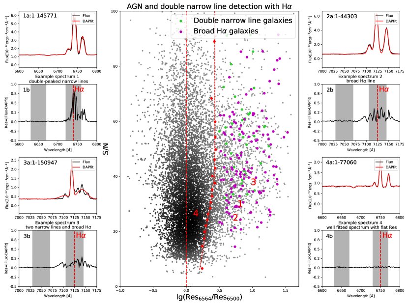
Figure 1: Normalized residual distribution vs. mean g-band signal-to-noise-ratio. The red dots represent 1$\sigma$ cuts of normalized residual in 20 S/N bins, with the red dashed line indicating the trend of the division. The coloured dots shows how the broad $\rm H\alpha$ and double-peaked narrow line galaxies are distributed according to our results in Section 3.4. The eight adjacent panels are from four different galaxies and demonstrate three dominant multi-Gaussian features: 1) double-peaked narrow $\rm H\alpha$ line, 2) broad $\rm H\alpha$ line, 3) double-peaked narrow $\rm H\alpha$ line and broad line, and 4) a well-fitted spectrum. The flux (a) and residuals (b) are shown two in a group. The shaded part of spectra indicates the area affected by the $\rm H\alpha$ line and area used to calculate $\rm Res_{6500}$.

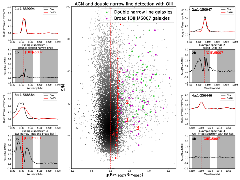
Figure 2: Normalized residual distribution vs. mean g-band signal-to-noise-ratio. The red dots represent 1$\sigma$ cuts of normalized residual in 20 ($S/N$) bins, with the red dashed line indicating the trend of the division. The coloured dots shows how the broad [OIII]$\rm\lambda$5007 and double-peaked narrow line galaxies are distributed according to our results in Section 3.4. It should be noted that the double-peaked narrow line galaxies are the same galaxies shown in Fig. 1 because double-peaked narrow line feature appears in every emission line. The eight adjacent panels are from four different galaxies and demonstrate three dominant multi-Gaussian features: 1) double-peaked narrow [OIII]$\rm\lambda$5007 line, 2) broad [OIII]$\rm\lambda$5007 line, 3) double-peaked narrow [OIII]$\rm\lambda$5007 line and broad line, and 4) a well-fitted spectrum. The flux (a) and residuals (b) are shown two in a group. The shaded part of spectra indicates the area affected by the [OIII]$\rm\lambda$5007 line and area used to calculate $\rm Res_{5060}$.

2.1 The MaNGA Survey

The MaNGA survey (Bundy et al., 2015) is an integral field unit (IFU) survey providing a three-dimensional view of galaxies. MaNGA data includes a sample of 10010 high-quality unique galaxy observations with spatially resolved spectra within the redshift range of 0.01 < z < 0.15 (Wake et al., 2017). The spaxel size of MaNGA is 0.5" and the average g-band Point Spread Function (PSF) FWHM (full width at half maximum) throughout the survey is about 2.54" (Law et al., 2016).

The spectra provided by MaNGA cover a wavelength range of 3600 to 10300 Å  at a spectral resolution of $\rm\sigma$ = 72 km/s (Law et al., 2016). Raw spectra are processed by the Data Reduction Pipeline (DRP) and products such as stellar continuum and emission line properties are produced by the Data Analysis Pipline (DAP) (Law et al., 2016; Westfall et al., 2019; Belfiore et al., 2019).

2.2 Selection Based on Normalized Residual

In total, we have 10010 high-quality unique galaxy observations from DR17, the final release of MaNGA, with MaNGA DAP outputs. An empirical way of assessing line detection is using the amplitude over noise ratio ($(A/N)_{\rm line}>3$) acquired from the DAP emission line modeling procedure (Belfiore et al., 2019). It is safe to remove 293 galaxies with a maximum $(A/N)_{\rm line}<3$ because there are no emission line detection in these galaxies. That leaves only 9717 galaxies to measure the fit quality of the emission line model.

A DAP residual is introduced to represent the fit quality of the spectrum. The DAP residual is defined as the absolute value of the difference between the DAP model and the actual flux data:

$$\rm Residual=|DAPModel-Flux|.$$ (1)

The residual of a given wavelength is calculated from the median residual within a range of $\pm$20Å  around the wavelength. The emission line residual is normalized by comparing it with the residual at an adjacent wavelength in the same spectrum without emission lines. We use the normalized residual of two typical emission lines, $\rm H\alpha$ and [OIII]$\rm\lambda$5007, to represent the fit quality of emission lines. $\rm H\alpha$ is the strongest emission line in the Balmer series and the broad $\rm H\alpha$ line is the most prominent feature of type-1 AGNs while [OIII] $\rm\lambda$5007 is usually a relatively strong forbidden line in 4000Å$\sim$ 8000Å  with no contamination from other emission lines close to it. The normalized residual of $\rm H{\alpha}$ (6564Å) is calculated through equation (missing) 2 and the normalized residual of [OIII]$\rm\lambda$5007 is calculated through equation (missing) 3.

$$\frac{\rm Res_{6564}}{\rm Res_{6500}}=\frac{{\rm Median\,Residuals\,within}\,(1+z)\times[6544,6584]\mbox{\AA}}{{\rm Median\,Residuals\,within}\,(1+z)\times[6480,6520]\mbox{\AA}}.$$ (2)

$$\frac{\rm Res_{5007}}{\rm Res_{5060}}=\frac{{\rm Median\,Residuals\,within}\,(1+z)\times[4987,5027]\mbox{\AA}}{{\rm Median\,Residuals\,within}\,(1+z)\times[5040,5080]\mbox{\AA}}.$$ (3)

Ideally, we will expect the normalized residual to be roughly 1, or slightly larger due to the increased photon noise due to the emission, which means the spectra of the emission lines are as well-fitted as anywhere else in a spectrum. The galaxies are divided uniformly into 20 signal-to-noise ratio ($S/N$) bins according to their mean g-band weighted signal-to-noise ratio. The middle panel in Fig. 1 shows the distribution of normalized residual in galaxies with $(A/N)_{\rm H\alpha}>3$. The red dots represent the position of 1$\rm\sigma$ cut in each ($S/N$) bin. A total of 17% of galaxies have a residual ratio above this cut. The ordinate of each point represents the median ($S/N$) in its corresponding bin. The dashed line only represents the division trend. The figure shows that the 1$\sigma$ residual cuts increase with the increase of ($S/N$) for $S/N<40$. That is because brighter galaxies with stronger $\rm H\alpha$ emission have larger ($S/N$). These galaxies have larger residuals within certain ($S/N$) range. The outliers to the right of the red dots are candidates for searching broad $\rm H\alpha$ and double-peaked narrow line features.

Fig. 2 shows the distribution of normalized residual vs. ($S/N$) for [OIII] $\rm\lambda$5007 in galaxies with $(A/N)_{\rm H\alpha}>3$. The structure and labels of image is consistent with Fig. 1. It should be noted that the number of outliers in the [OIII] $\rm\lambda$5007 region is much smaller than that of the former $\rm H\alpha$ outliers. That is because only a fraction of type-1 AGNs shows broad [OIII] feature.

We select the galaxies to the right of the 1$\rm\sigma$ cuts in Fig. 1 and Fig. 2. There are 1652 different galaxies. The flowchart in Fig. 3 shows the number of objects that survived each selection.

Figure 3: Number of objects survived after each selection step.

3 Methods

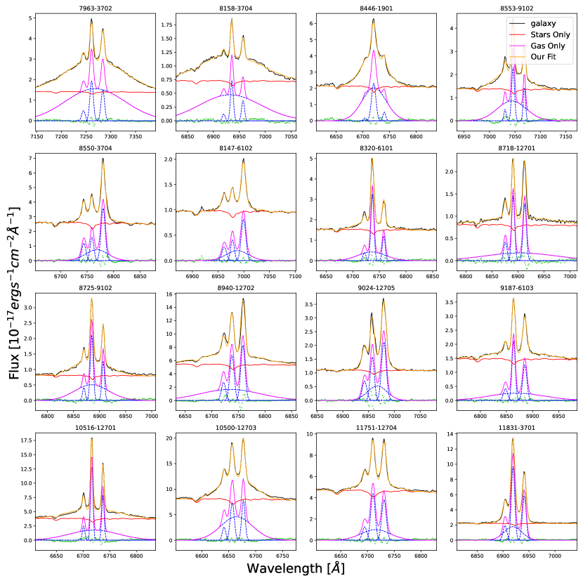
Figure 4: Examples of galaxies with broad $\rm H\alpha$ lines. The black spectra are the observed galaxy flux in $\rm H\alpha$ region. The orange spectra are our multi-Gaussian fit. In the lower half of the picture, the green dots represent the residual of multi-Gaussian fit. Individual Gaussian line fitting is shown in dashed blue lines. The total flux of gas and stellar are shown in magenta and red lines.

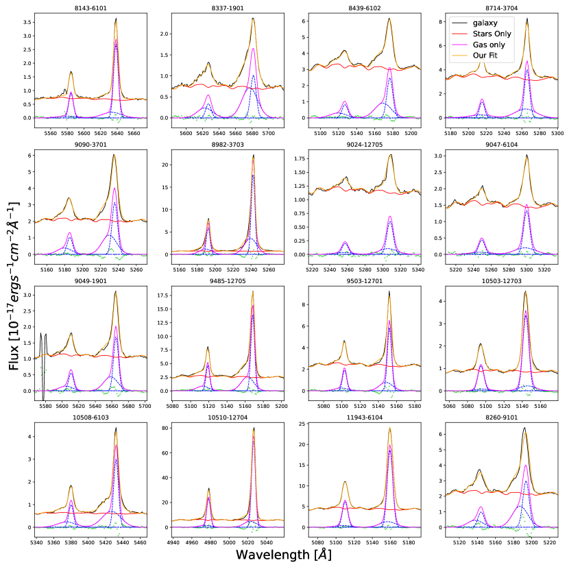
Figure 5: Examples of galaxies with broad $\rm[OIII]$ doublets. Correspondence between spectrum and colour is described in Fig. 4.

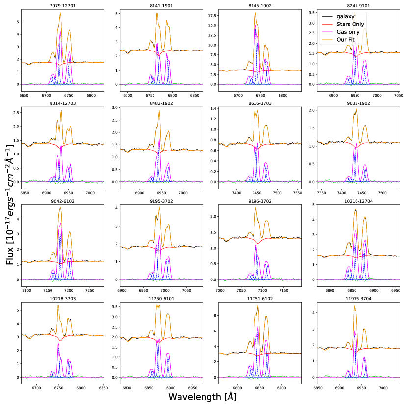
Figure 6: Examples of galaxies with double-peaked narrow lines. Correspondence between spectrum and colour is described in Fig. 4.

In this section, we show how we fit the multi-Gaussian emission line features with the help of ppxf software. In Section 3.1, we will first briefly introduce ppxf. In Section 3.2, we describe the kinematic constraints on broad and narrow emission lines. In Section 3.3, we acquire new stellar kinematics in a few galaxies where the DAP stellar continuum are not accurate due to the pollution of the broad lines.

3.1 The ppxf software

Our emission line model is based on the latest version of ppxf (Cappellari & Emsellem, 2004; Cappellari, 2017, 2022). This penalized pixel-fitting (ppxf) software pioneered a robust pixel-fitting method, particularly optimized for extracting the kinematics of the stars and gas in galaxies from integral-field spectroscopic (IFS) data.

When modeling gas emission lines, ppxf fits the gas emission lines together with the stellar kinematics. Multiple Gaussian emission lines can be fitted by passing to the program an arbitrary number of Gaussian emission line templates. The kinematics of lines can be tied to each other, or they can be fitted independently. And the relative fluxes of emission line doublets can be fixed or fitted independently. Detailed constraints applied in this paper are described in the following section.

3.2 kinematic constraints for the gas emission lines

For the 1652 1$\sigma$ outliers identified in Section 2, we opted not to make the multi-Gaussian fitting too complex and risk losing physical significance. Therefore, we assumed three multi-Gaussian models, each of which corresponds to different dynamic processes and is limited by different kinematic constraints. Specifically, the models contained either (1) broad Balmer lines, (2) broad Balmer and broad [OIII] lines, or (3) double-peaked narrow lines. We then selected the best fit model for each outlier and obtained the corresponding line properties.

Depending on the presence of broad [OIII] doublets, Table 1, Table 2, and Table 3 demonstrates the gas kinetic constraints on emission lines during our fitting. Lines included in gas kinematic component are given in the Tables and are fitted with the same velocity and dispersion. Table 1 shows the kinematic constraints in galaxies with broad balmer emission lines including broad $\rm H\delta$, $\rm H\gamma$, $\rm H\beta$ and $\rm H\alpha$. We use three different sets of emission line templates: (i) Narrow Balmer, (ii) Broad Balmer and (iii) Narrow forbidden. We use the ‘constr_kinem’ keyword in ppxf to set linear constraints on the emission line kinematics. We limit the velocity difference of broad and narrow Balmer lines to be less than broad line velocity dispersion to ensure the emission lines are at the corresponding wavelength. And the velocity dispersion of broad lines should be at least 600km/s larger than that of narrow lines to separate them apart.

Table 1: Kinematic constraints in Galaxies with broad Balmer emission lines.

Template name	Lines included	Kinematic parameters
Narrow Balmer	$\rm H\delta$,  $\rm H\gamma$, $\rm H\beta$,  $\rm H\alpha$	$\rm V=V_{1}$,  $\rm\sigma=\sigma_{1}$
Broad Balmer	$\rm H\delta$,  $\rm H\gamma$,  $\rm H\beta$,  $\rm H\alpha$	$\rm V=V_{2}$, $\rm\sigma=\sigma_{2}$
Narrow forbidden	$\rm[OIII]$,  $\rm[NII]$,  $\rm[SII]$	$\rm V=V_{3}$, $\rm\sigma=\sigma_{3}$

constraints: $|V_{1}-V_{2}|<\sigma_{2}$, $\sigma_{2}>\sigma_{1}+600$ km s^-1

Table 2 shows the kinematic constraints in galaxies with broad balmer and broad [OIII] emission. Here we add an extra broad [OIII] template. While still using the dynamic restrictions on the broad Balmer lines, we limit the velocity difference of broad and narrow [OIII] lines to be less than broad line velocity dispersion. And the velocity dispersion of broad [OIII] should be at least 300 km/s larger than that of narrow forbidden lines.

Table 2: Kinematic constraints in Galaxies with broad [OIII] and broad Balmer emission lines

Template name	Lines included	Kinematic parameters
Narrow Balmer	$\rm H\delta$, $\rm H\gamma$, $\rm H\beta$, $\rm H\alpha$	$\rm V=V_{1}$, $\rm\sigma=\sigma_{1}$
Broad Balmer	$\rm H\delta$, $\rm H\gamma$, $\rm H\beta$, $\rm H\alpha$	$\rm V=V_{2}$, $\rm\sigma=\sigma_{2}$
Narrow forbidden	$\rm[OIII]$, $\rm[NII]$, $\rm[SII]$	$\rm V=V_{3}$, $\rm\sigma=\sigma_{3}$
Broad [OIII]	[OIII]4960, [OIII]5007	$\rm V=V_{4}$, $\rm\sigma=\sigma_{4}$

constraints:$|V_{1}-V_{2}|<\sigma_{2}$,  $\sigma_{2}>\sigma_{1}+600$ km s^-1,  $|V_{3}-V_{4}|<\sigma_{2}$

Table 3 shows the kinematic constraints in galaxies with double narrow lines emission. For Balmer lines and forbidden lines, two sets of templates are given to each set of lines. We limit the velocity difference of the same lines in different templates to be larger than three times the velocity dispersion to ensure they are separated apart.

Table 3: Kinematic constraints in Galaxies with double-peaked narrow lines.

Template name	Lines include	Kinematic parameters
Narrow Balmer 1	$\rm H\delta$, $\rm H\gamma$, $\rm H\beta$, $\rm H\alpha$	$\rm V=V_{1}$, $\rm\sigma=\sigma_{1}$
Narrow Balmer 2	$\rm H\delta$, $\rm H\gamma$, $\rm H\beta$, $\rm H\alpha$	$\rm V=V_{1}$, $\rm\sigma=\sigma_{2}$
Narrow forbidden 1	$\rm[OIII]$, $\rm[NII]$, $\rm[SII]$	$\rm V=V_{3}$, $\rm\sigma=\sigma_{3}$
Narrow forbidden 2	$\rm[OIII]$, $\rm[NII]$, $\rm[SII]$	$\rm V=V_{4}$, $\rm\sigma=\sigma_{4}$

constraints: $V_{1}-V_{2}>72$ km s^-1,  $V_{3}-V_{4}>72$ km s^-1.

The possible combination of double-peaked narrow line and broad line is not included in Table 1, Table 2, and Table 3. We find only one galaxy with such rare emission line feature. The galaxy is fitted manually and we will discuss its dynamic features in detail in Section 4.5.

For the majority of galaxies we adopt the stellar continuum provided by DAP. So we do not fit polynomials with ppxf. In a few cases, the width of the broad line affects the stellar continuum fitting of the DAP. These cases are discussed in Section 3.3. Fig. 4, Fig. 5 and Fig. 6, show examples of broad $\rm H\alpha$ or dual narrow line fitting. We did not fit for attenuation here. And considering the time taken, we did not perform a global optimization with ppxf keyword ‘globel_search’ on every galaxy. However, we compared the convergence in our fits for broad line galaxies with the global optimized fits using ‘globel_search’ and find little difference between them. Detailed emission line properties and galaxy information can be found in appendix A.

3.3 Stellar kinematic of galaxies with very broad emission

The presence of broad emission lines also affects the stellar kinematics produced by DAP, which masks the emission lines according to a specific width of 800 km/s and determines the stellar kinematics using the rest of the spectrum (Westfall et al., 2019). The width is insufficient for broad emission lines, especially broad Balmer lines with typical with of $\sim$1000 km/s. Insufficient masking of the emission line area leads to inaccurate kinetic properties in some spaxels.

After examining the broad-line galaxies, those galaxies where $\rm H\alpha$ lines width are around 1000 km/s are not much affected because nearby [NII] doublets help mask the entire $\rm H\alpha$ region in the spectrum. We acquire the new stellar continuum of the galaxies where broad $\rm\sigma_{H\alpha}$ > 1200 km/s by masking broad-line regions in spectra. Three examples are shown in Fig. 7.

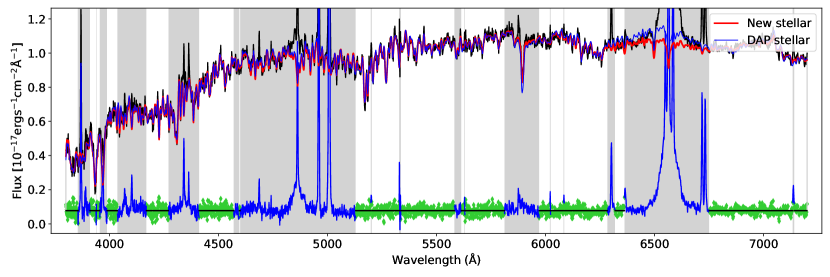
Figure 7: Example fit to the stellar continuum with ppxf to extract the stellar kinematics (MaNGA-ID: 1-495383, 1-53093 ,1-576315 from top to bottom). The shaded areas are those that are blocked due to the influence of the broad line. A typical width of broad Balmer lines in these severely affected galaxies is broad $\rm\sigma_{H\alpha}\sim$ 1500 km/s. We masked a 3$\rm\sigma$ range of $\pm$4500 km/s around $\rm H\alpha$ and a 2$\rm\sigma$ range of $\pm$3000 km/s around $\rm H\gamma$ and $\rm H\delta$. Finally, the $\rm H\beta$ and [OIII] region is masked completely within $\pm$6000 km/s around $\rm H\beta$ because this region is heavily contaminated. The black lines are the actual spectra. The blue lines to the top are the stellar continuum from DAP. The red lines are our new stellar continuum. The unnatural protrusions in $\rm H\alpha$ area disappear. The green diamond point shows the residuals which exclude the masked emission lines.

In the process of fitting the new galaxy continuum, we also obtain new values for stellar kinematic properties. Only in some of these galaxies, they are very different from DAP stellar kinematic properties. Fig. 8 gives an example.

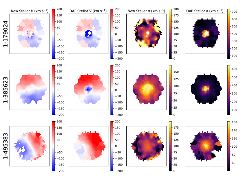
Figure 8: Comparison of stellar kinematics maps between our fits and DAP. The MaNGA-IDs of the three example galaxies are shown to the left of each row. Our fits have eliminated the apparently unphysical negative velocities in the broad line region at the center of the galaxy (As can be seen from the first two rows) and corrected the asymmetry in velocity maps due to wrong velocity in center spaxels influenced by AGNs. (As can be seen from the last row)

3.4 Fitting Result

We create a catalogue containing multi-Gaussian line properties of MaNGA galaxies derived from ppxf method. Table 4 reports how we present our results.

Table 4 and Table 5 gives 10 example galaxies. The luminosity ratio is measured using the apparent luminosities of two narrow $\rm H_{\alpha}$ components. Using $L_{\rm H\alpha}$ with larger velocity as numerator divide by $L_{\rm H\alpha}$ with smaller velocity as denominator. And $\Delta V$ is the absolute velocity difference measure from the center of the velocity. An entire catalogue can be found in appendix A. Comparing our broad line galaxies with the previous samples of type-1 AGNs in Sánchez et al. (2022). We recovered broad lines for 104 of the 119 type-1 AGN candidates in Sánchez et al. (2022), and we discovered 35 new galaxies with broad emission lines. For the rest 15 examples in Sánchez et al. (2022), we believe that these galaxies only have narrow lines with relatively larger velocity dispersion ($\sim$250km/s). We did not find broad Balmer emission lines. They are actually type-2 AGN candidates misclassified as type-1.

Table 4: Example catalogue of 5 galaxies with broad line features in MaNGA. A machine-readable version of the full table is available (see Supporting Information).

MaNGA-ID	RA	Dec	$\lg L^{\rm broad}_{H\alpha}$	$\lg\sigma^{\rm broad}_{H\alpha}$	$\lg\sigma_{\rm e}$	Extra templates
	(deg)	(deg)	( $10^{40}$erg s-1)	(km s-1)	(km s-1)
1-382273	118.634242	16.809729	12.91	3.403	2.137	Broad H$\alpha$
1-547191	258.118529	35.884086	14.71	3.251	1.954	Broad Balmer
1-300461	137.160233	32.592953	6.31	3.098	2.114	Broad H$\alpha$
1-587259	160.228870	5.991890	12.61	2.951	1.964	Broad H$\alpha$,[OIII]
1-150947	183.263995	51.648597	47.03	2.958	2.332	Broad H$\alpha$,[OIII]

• Note: Column (1) is the MaNGA identification ID. Column (2-3) is the position of the galaxy shown in celestial coordinates. We use the positions to acquire optical and radio images. Column (4) is the apparent luminosity of the broad $\rm H\alpha$ component. Column (5) is the flux-weighted velocity dispersion of the broad $\rm H\alpha$ component. Column (6) is the stellar velocity dispersion within 1Re corrected by masking the broad line region in Section 3.2. Column (7) shows the extra templates added when fitting each galaxy. The label ‘Broad H$\alpha$’ means in the broad Balmer set of templates the broad $\rm H\delta$, $\rm H\gamma$ and $\rm H\beta$ components are all zero or below the noise level. Only broad $\rm H\alpha$ is observable.

Table 5: Example catalogue of 5 galaxies with double narrow line features in MaNGA. A machine-readable version of the full table is available (see Supporting Information).

MaNGA-ID	Ra	Dec	Luminosity Ratio	$\lg\Delta V$ (km/s)	$\lg\sigma_{e}$ (km/s)	Extra templates
1-114955	332.602090	11.713077	1.91	2.444	2.433	Dual narrow
1-596678	332.892838	11.795929	0.53	2.358	2.130	Dual narrow
1-115365	333.483204	13.755396	1.10	2.391	1.982	Dual narrow
1-42007	33.626933	13.257206	1.61	2.367	2.057	Dual narrow
1-41752	31.953063	13.609595	3.01	2.330	2.233	Dual narrow

• Note: Column (1) is the MaNGA identification ID. Column (2-3) is the position of the galaxy shown in celestial coordinates. We use the positions to acquire optical and radio images. Column (4) is the apparent luminosity ratio measured through the double $\rm H\alpha$ components. Column (5) is the velocity difference between the two narrow components. Column (6) is the stellar velocity dispersion within 1Re. Column (7) shows the extra templates added when fitting each galaxy. The label ‘Dual narrow’ means adding an extra set of narrow lines with kinematic constrains from Table 3.

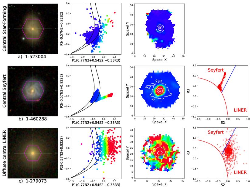
Figure 9: Examples of the different ionization levels in broad line galaxies. The first column is the galaxy images with MaNGA-ID labeled below. The second column is the classification based on equation (missing) 4. Each dot represents a single spaxel and the colour is based on its distance to $\rm 1\sigma$ line. The two solid black lines are the 1$\sigma$ and 3$\sigma$ limits of the AGN vs star forming separation by Law et al. (2021, Figure 15). The third column is a map of the galaxy colour-coded according to the position of individual regions with the same colour-coding as in the second column. Broad line areas are marked on the map as contours. The outermost contour represents all spaxels with broad $\rm H\alpha$. The innermost contour represents the position of the spaxel with the brightest broad $\rm H\alpha$. The contour in the middle represents the half maximum flux of the broad $\rm H\alpha$. The fourth column separate LINERs (red open circles) from Seyfert AGNs (red filled squares).

4 Results and discussions

In this section, we will discuss how galaxies with broad emission lines are characterized based on the emission line properties given in this paper. In Section 4.1, we will discuss the classification of broad-line galaxies on BPT diagrams. In Section 4.2 and Section 4.3, we want to study the AGN-galaxy coevolution through the stellar population of broad-line region host galaxies and the relation between broad lines’ properties and the host galaxies’ dynamical properties. In Section 4.4, we show examples of how the spatial distribution of broad emission lines can help us find AGN mergers.

4.1 BPT diagrams

For galaxies with broad emission lines, we not only fit the broad lines but also correct the misfit of the narrow line properties in DAP caused by the broad lines. The relative strengths of different narrow lines provide sensitive diagnostics of the properties of the ionized gas and the astrophysical processes in their host galaxies.

MaNGA’s observed wavelength range (3600 - 10300 Å) covers all the strong nebular lines used in the standard BPT diagram (Baldwin et al., 1981) in MaNGA redshift range (0.02<z<0.15) . Based on MaNGA data, Law et al. (2021) finds that the gas phase velocity dispersion correlates strongly with traditional optical emission line ratios such as [SII]/$\rm H\alpha$, [NII]/$\rm H\alpha$, and [OIII]/$\rm H\beta$. Henceforth we adopt the definition in Law et al. (2021) of some most widely used ratios such as $\rm\log([NII]\lambda 6585/H\alpha$) (hereafter ‘N2’), $\rm\log([SII]\lambda 6718+6732/H\alpha$) (hereafter ‘S2’), and $\rm\log([OIII]\lambda 5008/H\alpha$) (hereafter ‘R3’). The corresponding relation that separates the cold-disk sequence from the warm-disk sequence takes the form :

$$N2=\sum_{i=0}^{2}\sum_{j=0}^{2}C_{ij}S2^{i}R3^{j},$$ (4)

where $C_{ij}$s are the coefficients shown in Table 6.

Table 6: Coefficients of the polynomial surface in equation (missing) 4. This is Table 2 of Law et al. (2021).

$C_{ij}$	j = 0	1	2
i=0	$-$0.7362	$-$0.6464	$-$1.7567
1	$-$1.2338	$-$2.0170	1.3520
2	$-$0.3036	0.4533	0.3177

An edge-on projection of the interface is shown under coordinates $P1$, $P2$ where (Law et al., 2021, eq. 12-13).

$$P1=0.77\,N2+0.54\,S2+0.33\,R3.$$ (5)

$$P2=-0.57\,N2+0.82\,S2.$$ (6)

In Fig. 9, we illustrate the types of ionization structures observed in MaNGA galaxies and our classification scheme. The galaxy in Fig. 9a (MaNGA-ID: 1-523004) is a typical star-forming galaxy with broad $\rm H\alpha$ emission. Star-forming spaxels dominate the broad line region around its galactic nucleus.

The galaxies in Fig. 9b and Fig. 9c are Classified as AGN with broad $\rm H\alpha$ emission. AGN spaxels dominate the broad line region. Then we put spaxels that are classified as AGN in the S2 vs. R3 diagram and separate LINERs from Seyfert AGNs.

4.2 Stellar population of AGNs

One popular method to study the AGN-galaxy coevolution is via examining the stellar population of AGN host galaxies. Fig. 10 and Fig. 11 show the distribution of mass, effective radius, age, and metallicity of broad $\rm H\alpha$ galaxies classified into different categories by BPT diagram. The coloured dots in the background represent the distribution of all other MANGA galaxies under the same set of physical parameters. The stellar population properties used in this work is from Lu et al. (2023), which applies the ppxf (Cappellari, 2022) on the full sample in MaNGA project and derives their both global and spatially resolved stellar population properties (including stellar mass, metallicity, and age). The stellar masses used here are calculated within the elliptical half-light isophotes, taken from the catalogue of Lu et al. (2023) under the keyword ‘Mstar_Re’. The ages and metallicities are the SDSS $r-$band (Stoughton et al., 2002) luminosity-weighted average value within the half-light isophote under keyword ‘LW_Age_Re’ and ‘LW_Metal_Re’. The stellar velocity dispersions within 1Re come from DAPall file (Westfall et al., 2019) and the effective radius (Re) are half-light radius provided by the NSA catalogue. The NSA catalogue is an extension of the NASA-Sloan Atlas (NSA) toward higher redshift (z $\leq$ 0.15) and includes an elliptical Petrosian analysis of the surface-brightness distributions (Blanton et al., 2011).

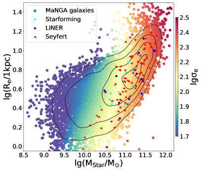
Figure 10: The distribution of mass vs. effective radius of broad $\rm H\alpha$ galaxies. The dots coloured by $\rm\sigma_{e}$ from DAP in the background represent the distribution of all other MANGA galaxies. Galaxies classified into different categories are represented using different colours. The contour lines are a kernel density estimate of the galaxies number density, computed with the Scipy (Virtanen et al., 2020) function scipy.stats.gaussian_kde. The velocity dispersion was smoothed using the LOESS procedure by Cappellari et al. (2013b), which implements the algorithm by Cleveland & Devlin (1988).

According to Fig. 10, AGN and star-forming triggered broad-line galaxies are scattered around the middle of the image. The host galaxies of LINER tend to have larger $\rm\sigma_{e}$ and more than half of them lie in the region of the elliptical galaxies to the upper right of the figure. This is consistent with the morphology observed from the images.

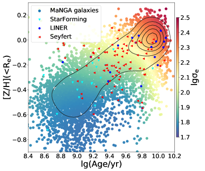
Figure 11: The distribution of age vs. metallicity of broad $\rm H\alpha$ galaxies. The colours and symbols are described in Fig. 10.

Fig. 11 shows that the star-forming galaxies are relatively young and LINER galaxies are old. The old ages of LINERS is consistent with previous studies who concluded that LINER emission is due to ionization by evolved stars (Sarzi et al., 2010; Yan & Blanton, 2012; Belfiore et al., 2016; Sánchez et al., 2021). Compared with the number density of MANGA galaxies, the distribution of AGN host galaxies are not concentrated in the upper-right region. Instead, they show a slightly scattered distribution in the middle. The AGN host galaxies occupy a large range of ages from old to young galaxies and they preferentially lie around intermediate ages. The finding corroborate previous results in Hernán-Caballero et al. (2014) and Georgantopoulos et al. (2023). The relatively young age of AGN host galaxies hints at the presence of a significant younger stellar population (Kauffmann et al., 2003; Sánchez et al., 2004) that is consistent with the result through color analyses (eg., Schawinski et al., 2014; Zhang et al., 2016).

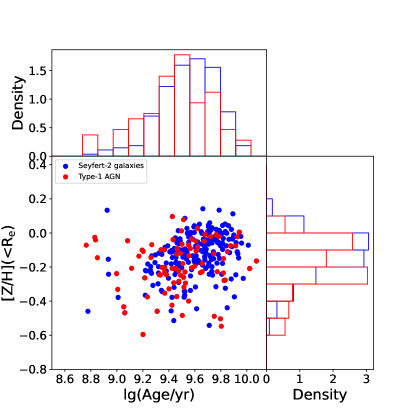
Figure 12: The distribution of age vs. metallicity of broad $\rm H\alpha$ type-1 AGNs and narrow line seyfert-2 galaxies.

Sánchez et al. (2021) described in detail the classification criterion for different sources of ionization using traditional BPT diagrams as well as the equivalent width of $\rm H\alpha$ and the spatial distribution of line ratios. An AGN ionized region is characterized by its emission line ratios well above the Kewley et al. (2001) demarcation lines and EW($\rm H\alpha$) larger than 3 Å. They present a decrease of the considered line ratios with respect to the central values in the galaxy and show a steep decline in the flux intensity (Sánchez, 2020; Sánchez et al., 2021). In most of our broad line galaxies, broad line regions largely coincide with AGN ionized regions. To further understand the role of the broad line in AGN ionized region, Fig. 12 shows the distribution of broad-line type-1 AGNs and narrow-line seyfert-2 host galaxies on the age-metallicity diagram. Due to the fact that AGN ionized region is mostly concentrated in the central regions (eg. Husemann et al., 2010, 2014; Sánchez, 2020) the seyfert-2 host galaxies are classified by applying the standard BPT diagram on the centre spaxel and obtaining the ‘seyfert’ classifications without broad lines as a first order approximation. Our work indicates that the host galaxy of type-1 AGNs are slightly younger than seyfert-2 galaxies. Their metallicity distribution follows the same trend. Georgantopoulos et al. (2023) recently explored the properties of the host galaxies of X-ray selected AGN in the COSMOS field using the Chandra Legacy sample and the LEGA-C survey VLT optical spectra. They measured the ages of different types of AGNs through $\rm D_{n}$4000. Our finding is consistent with their result.

4.3 Testing the $M_{\rm BH}-\sigma_{\rm e}$ relation in type-1 AGNs

Another way to study the AGN-galaxy coevolution is to connect broad lines’ properties to the galaxies’ dynamical properties. Greene & Ho (2005) suggested that the velocity dispersion and luminosity of broad lines have a strong correlation with black hole mass in active galactic nuclei. Meanwhile, the black hole mass is related to the stellar velocity dispersion within the effective radius ($\sigma_{e}$). Previously, the $M_{\rm BH}-\sigma_{\rm e}$ relation (Gebhardt et al., 2000; Ferrarese & Merritt, 2000) has been parameterized as a power-law function ($M_{\rm BH}\propto\sigma_{\rm e}^{\alpha}$) (e.g. Beifiori et al., 2012; McConnell & Ma, 2013; Kormendy & Ho, 2013; Woo et al., 2015; Caglar et al., 2020), where $\alpha$ was found to be between 3 and 6.

For type-1 AGN with broad H$\alpha$ lines, we used the prescription of Greene & Ho (2005, eq.6) :

$$M_{\rm BH}=2\times 10^{6}\left(\frac{L_{\rm broad\,H\alpha}}{\rm 10^{42}erg\,s^{-1}}\right)^{0.55}\left(\frac{{\rm FWHM}(H\alpha)}{1000\;\rm km/s}\right)^{2.06},$$ (7)

where ${\rm FWHM}(H\alpha)$ is calculated from the flux weighted average of broad $\rm H\alpha$ velocity dispersion in different spaxels. Notice that ${\rm FWHM}(H\alpha)=\sigma\sqrt{4\ln(4)}$. Section 3 provides the apparent luminosity of the broad $\rm H\alpha$ line. The attenuation-corrected $\rm H\alpha$ flux is obtained through equation (missing) 8:

$$L_{\rm broad\,H\alpha,corr}=L_{\rm broad\,H\alpha}10^{0.4A_{\rm H\alpha}},$$ (8)

where $A_{\rm H\alpha}=3.33\;E(B-V)$ according to Domínguez et al. (2013, eq 1,6).

We measure E(B$-$V) from the Balmer decrement (Domínguez et al., 2013, eq 4) :

$$E(B-V)=1.97\;\lg\left[\frac{\rm(H\alpha/H\beta)_{obs}}{2.86}\right].$$ (9)

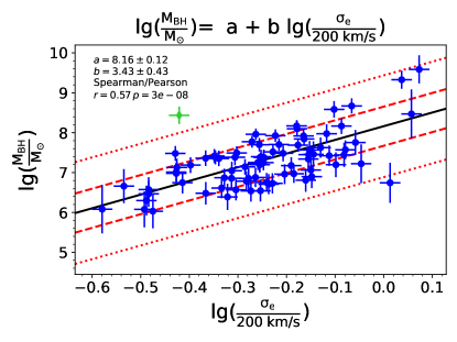
Figure 13: The $M_{\rm BH}-\sigma_{\rm e}$ relation in MaNGA type-1 AGNs. The blue dots are $\rm M_{BH}$ and $\rm\sigma_{e}$ of type-1 AGN with errorbar. The dashed red lines represent the 1$\sigma$ (68%) and 2.6$\sigma$ (99%) error range of the linear fit. The green dot is not included as it falls outside the range of fitting error. The fitting result is represented by the solid black line, while the fitting parameters, the Spearman-Pearson correlation value, and the probability of no correlation are displayed in the upper left corner of the figure.

In Fig. 13, we test the $\rm M_{BH}$-$\rm\sigma_{e}$ relation in our type-1 AGN catalogue. For the fit we used the lts_linefit procedure by Cappellari et al. (2013a) which combines the Least Trimmed Squares robust technique by Rousseeuw & Van Driessen (2006) into a least-squares fitting algorithm. The procedure allows for errors in both variables and intrinsic scatter. We present our result in equation (missing) 10 :

$$\lg\left(\frac{M_{\rm BH}}{M_{\rm\odot}}\right)=(8.16\pm 0.12)+(3.43\pm 0.43)\lg\left(\frac{\sigma_{\rm e}}{\rm 200km/s}\right).$$ (10)

Our result matches with the recent $M_{\rm BH}-\sigma_{\rm e}$ relation in equation (missing) 11 given by Caglar et al. (2020, eq.14) :

$$\lg\left(\frac{M_{\rm BH}}{M_{\rm\odot}}\right)=(8.14\pm 0.20)+(3.38\pm 0.65)\lg\left(\frac{\sigma_{\rm e}}{\rm 200km/s}\right).$$ (11)

And the slope of our result is within the allowable range of Woo et al. (2015) ($3.97\pm 0.56$).

4.4 Discovery of dual AGNs

The multiple supermassive black holes are expected to exist inside many galaxies due to the previous merging events. They can be revealed by the detection of the coexistence of two active galactic nuclei in the merging system of galaxies (Mannucci et al., 2022). Recently, Hernández-Toledo et al. (2023) studied the incidence of major mergers and their impact on the triggering of AGN activities using MaNGA DR15 sample. Building a large sample of local dual AGNs amongst merging galaxies helps understand how the merging process of some galaxies excite galactic nuclei and convert them into AGN (Capelo et al., 2017; Chen et al., 2022).

The currently largest catalogue of 36 dual AGNs (including 31 new findings and 5 previous cases) comes from Zhang et al. (2021a, b). Such events are hard to identify and require high spatial resolution data to determine the presence of two AGNs in a galaxy rather than one large-scale AGN. We use a combination of broad $\rm H\alpha$ flux map and radio map from the VLA FIRST survey (Becker et al., 1995) to confirm our detection of dual AGNs in MaNGA. In Fig. 14 and Fig. 15, we present two dual AGN mergers with clear bimodal radio features. In Fig. 16, we present a dual AGN candidate where the two galaxies are too close to be separated on the radio map. But there is a clear bimodal feature on the broad $\rm H\alpha$ flux map.

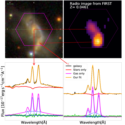
Figure 14: Image and emission line fitting result for dual AGN candidates (MaNGA-ID: 1-382273). The upper left panel is the galaxy image from MaNGA. The upper right panel shows the radio image from the FIRST radio survey (Becker et al., 1995). We can see a clear bimodal feature. Redshift and separation measured from flux centre is labeled on the radio image. The two images below show $\rm H\alpha$ fitting at the centres. The green dots represent the residual of multi-Gaussian fit.

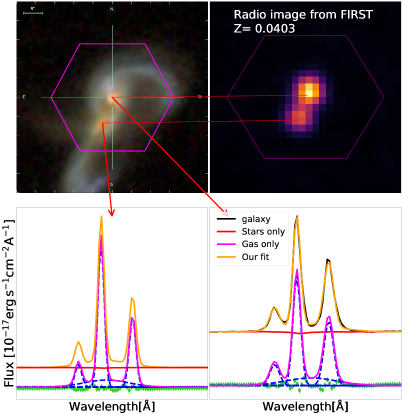
Figure 15: Image and emission line fitting result for dual AGN candidates (MaNGA-ID: 1-585513). The symbols are the same as in Fig. 14.

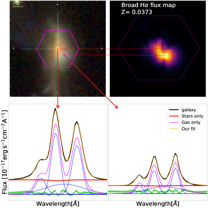
Figure 16: Image and emission line fitting result for dual AGN candidates (MaNGA-ID: 1-244377). The upper left panel is the galaxy image from MaNGA. The upper right panel is the map of broad $\rm H\alpha$ flux. The two galaxies are too close to be separated on the radio map. The two images below shows $\rm H\alpha$ fitting at the centres.

Detection of such dual AGN events will help us to further understand the role of active galactic nuclei in galaxy evolution. In future work, it is possible to further investigate what kind of galactic nuclei will be excited as AGNs in mergers and how dual AGNs can form in the future.

4.5 A combination of broad $\rm H\alpha$ and double narrow lines

In Section 3, we use different templates to fit different multi-Gaussian features. We usually assume broad lines and double narrow lines are caused by different mechanisms. So we did not discuss the cases where they occur simultaneously. To the bottom right of Fig. 1 and Fig. 2, we still notice such feature in the spectrum of a merger sample shown in Fig. 17.

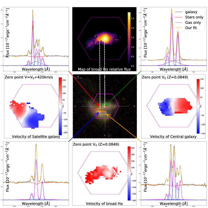
Figure 17: The case where broad H$\alpha$ and double narrow line features occur simultaneously. The MaNGA-ID of the object is 1-150947. The panels on the four corners represent the $\rm H\alpha$ spectra at different locations of the galaxy. The central box is its optical image. The panel on top of the optical image is the map of relative broad $\rm H\alpha$ flux and the panel at the bottom is the map of broad $\rm H\alpha$ velocity. The panels to the left and right are the narrow-line velocity maps of the central and satellite galaxy.

According to the velocity maps of the central and satellite galaxy, the velocity at the satellite galaxy centre is 420 km/s larger than that of the central galaxy. The broad $\rm H\alpha$ velocity map shows that the broad $\rm H\alpha$ velocity in region where broad H$\alpha$ and double narrow line features occur simultaneously (red region on optical image) follows the velocity of the satellite galaxy. This suggests that the broad lines in the region and the central broad lines (green region) may come from different physical processes. One possible explanation is that in the overlapping area, there are three separated gas region along line of sight. One comes from the satellite galaxy and produces the narrow-line set with larger velocity. One comes from the central galaxy and produces the narrow-line set with lower velocity. And a region between them dominated by shock waves triggered by merging. But there is a possibility of a wandering black hole accreting in the overlapping region. This needs to be tested with higher resolution X-ray or radio images in future work.

5 Summary

We have carried a systematic search for broad $\rm H\alpha$ and double-peaked narrow emission line features in the full MaNGA sample. Galaxies with $\rm H\alpha$ amplitude over noise ratio in larger than three are divided uniformly according to their mean g-band weighted signal-to-noise ratios. We identified 188 galaxies where single Gaussian emission line fits fail among 1$\rm\sigma$ outliers in each bin. There are 38 galaxies with broad $\rm H\alpha$ and [OIII] $\rm\lambda$5007 lines, 101 galaxies with broad $\rm H\alpha$ lines but no broad [OIII] $\rm\lambda$5007 lines, and 49 galaxies with double-peaked narrow emission lines. New emission line properties (including velocities, velocity dispersions, flux) are obtained by fitting multi-Gaussian templates in ppxf (Cappellari, 2022) with kinematic constraints on broad and narrow components. The galaxies with broad emission lines are classified into three catagories : central star-forming, central AGN, and diffuse central LINER according to their BPT diagram.

The catalogue helps us further understand the AGN-galaxy coevolution through the stellar population of broad-line region host galaxies and connecting broad lines’ properties to the host galaxies’ dynamical properties. type-1 AGN occupy the full range of ages from old systems to young galaxies. The star-forming galaxies are relatively young and LINER galaxies are usually old. Our work indicates that the host galaxy of type-1 AGNs are slightly younger than seyfert-2 galaxies while their metallicity distribution follows the same trend. This is consistent with results recently reported in Georgantopoulos et al. (2023).

We estimate the masses of black hole in type-1 AGN through broad $\rm H\alpha$ width and luminosity based on the formula given by Greene & Ho (2005). Using the $\sigma_{\rm e}$ from DAP, we obtain our $M_{\rm BH}-\sigma_{\rm e}$ relation for type-1 AGN in equation (missing) 10. Finally, we discover three dual AGN candidates in mergers in Section 4.4 and present one possible candidate for a wandering black hole in Section 4.5. This sample may be useful for further studies on AGN activities, feedback processes and their connections to stellar populations and dynamical properties.

Data Availability

The data underlying this article are available in the article and in its online supplementary material.

Appendix A The complete catalogue of galaxies with broad line or double narrow line features in MaNGA

Table 7: The complete catalogue of galaxies with broad line features in MaNGA

MaNGA-ID	RA	Dec	$\lg L^{\rm broad}_{H\alpha}$	$\lg\sigma^{\rm broad}_{H\alpha}$	$\lg\sigma_{\rm e}$	Extra templates
	(deg)	(deg)	( $10^{40}$erg s-1)	(km s-1)	(km s-1)
1-382273	118.634242	16.809729	12.91	3.403	2.137	Broad H$\alpha$
1-547191	258.118529	35.884086	14.71	3.251	1.954	Broad Balmer
1-300461	137.160233	32.592953	6.31	3.098	2.114	Broad H$\alpha$
1-587259	160.228870	5.991890	12.61	2.951	1.964	Broad H$\alpha$,[OIII]
1-150947	183.263995	51.648597	47.03	2.958	2.332	Broad H$\alpha$,[OIII]
1-60653	150.529327	3.057686	6.48	3.270	1.996	Broad H$\alpha$
1-78719	151.006758	4.051176	4.02	2.843	1.785	Broad H$\alpha$
1-3050	160.143696	0.817429	11.29	3.364	2.137	Broad H$\alpha$
1-181172	140.011912	5.735586	2.21	2.928	2.045	Broad H$\alpha$
1-180998	141.915721	5.053476	38.26	2.981	2.143	Broad H$\alpha$,[OIII]
1-244377	206.175720	55.887093	53.05	2.925	2.358	Broad H$\alpha$,[OIII]
1-218981	127.784888	30.895607	5.22	2.907	2.061	Broad H$\alpha$
1-301330	145.829803	36.247822	2.50	2.945	2.274	Broad H$\alpha$,[OIII]
1-301090	146.628758	34.916838	13.15	2.841	1.892	Broad H$\alpha$
1-567397	145.267159	34.732879	13.66	3.156	2.188	Broad H$\alpha$
1-282637	187.964780	43.245526	2.99	2.899	2.022	Broad H$\alpha$
1-195337	194.915701	53.341186	7.01	2.953	2.312	Broad H$\alpha$
1-320796	214.930149	49.236646	3.75	2.837	1.940	Broad H$\alpha$
1-623700	195.169935	52.537742	10.47	2.862	1.988	Broad H$\alpha$,[OIII]
1-135812	250.292722	38.831981	4.49	3.023	2.001	Broad H$\alpha$
1-136044	252.289916	36.223838	8.28	3.040	2.292	Broad H$\alpha$
1-336095	234.082184	9.344213	1.77	2.865	1.973	Broad H$\alpha$,[OIII]
1-294864	250.281830	22.823568	1.57	2.913	1.820	Broad H$\alpha$
1-96451	311.310818	-5.484327	5.90	2.854	2.057	Broad H$\alpha$
1-635845	328.577920	0.355400	8.30	2.906	1.908	Broad H$\alpha$,[OIII]
1-53288	134.619164	0.023460	2.64	2.908	1.914	Broad H$\alpha$,[OIII]
1-212706	325.590823	-8.364872	4.44	3.077	1.845	Broad H$\alpha$
1-98401	328.108473	-8.173600	13.94	2.998	2.134	Broad H$\alpha$,[OIII]
1-113405	316.841308	11.066421	1.71	3.247	1.903	Broad H$\alpha$
1-24148	258.827410	57.658770	2.46	3.262	2.041	Broad H$\alpha$
1-22948	254.542084	62.415648	16.68	2.919	2.111	Broad H$\alpha$,[OIII]
1-109378	51.169918	-0.681473	13.74	2.850	1.914	Broad H$\alpha$
1-39759	12.413884	13.685225	14.67	2.986	2.161	Broad H$\alpha$,[OIII]
1-39615	11.876450	15.697081	3.54	3.368	2.041	Broad H$\alpha$
1-548024	111.733682	41.026691	29.12	3.410	2.212	Broad H$\alpha$
1-338922	114.775747	44.402765	8.84	2.848	2.320	Broad H$\alpha$
1-72322	121.014201	40.802613	29.88	3.006	2.328	Broad H$\alpha$,[OIII]
1-121075	114.695391	29.891283	18.77	3.064	2.188	Broad H$\alpha$
1-163831	118.627843	25.815986	5.12	2.966	1.959	Broad H$\alpha$
1-460288	126.059633	17.331951	6.29	2.908	1.886	Broad H$\alpha$,[OIII]
1-460812	127.170800	17.581400	6.68	3.303	2.220	Broad H$\alpha$
1-585513	138.981378	44.332761	6.76	2.869	2.037	Broad H$\alpha$
1-258373	182.286727	44.003165	5.41	2.994	1.973	Broad H$\alpha$,[OIII]
1-558912	166.129408	42.624554	24.44	2.874	2.375	Broad H$\alpha$,[OIII]
1-284293	197.239319	45.905447	53.19	2.901	2.253	Broad H$\alpha$
1-575726	198.958904	46.338830	6.17	2.949	2.140	Broad H$\alpha$
1-261280	214.096447	38.190986	18.18	2.898	2.097	Broad H$\alpha$,[OIII]
1-155975	142.778168	49.079746	6.17	3.020	2.083	Broad H$\alpha$,[OIII]
1-166919	146.709100	43.423843	9.84	3.019	2.149	Broad H$\alpha$
1-211311	248.426386	39.185120	11.82	2.932	1.934	Broad H$\alpha$
1-576292	225.691343	53.512170	4.31	2.970	2.117	Broad H$\alpha$
1-198182	224.749647	48.409855	5.32	2.936	2.316	Broad H$\alpha$
1-569169	247.048171	39.821898	2.29	2.934	2.025	Broad H$\alpha$
1-594493	247.159333	39.551266	8.56	3.059	2.587	Broad H$\alpha$
1-95585	255.029870	37.839502	7.82	3.387	2.029	Broad H$\alpha$
1-546819	257.001371	36.344421	3.48	3.082	2.336	Broad H$\alpha$
1-114820	330.423500	11.856788	2.46	2.883	2.260	Broad H$\alpha$
1-24142	258.845726	57.411184	3.38	3.189	2.471	Broad H$\alpha$
1-604860	118.184153	45.949276	13.21	3.477	2.026	Broad H$\alpha$,[OIII]
1-604907	119.920672	50.839973	92.44	2.941	2.155	Broad H$\alpha$,[OIII]
1-44303	119.182152	44.856709	4.02	3.314	1.869	Broad H$\alpha$
1-44379	120.700706	45.034554	3.24	2.894	1.996	Broad H$\alpha$
1-47409	130.407776	54.918571	8.95	3.077	2.111	Broad H$\alpha$
1-574519	127.178094	45.742555	5.09	3.129	2.013	Broad H$\alpha$
1-163966	120.087418	26.613527	7.84	3.339	2.124	Broad H$\alpha$
1-279073	170.588145	46.430504	11.47	2.921	2.346	Broad H$\alpha$
1-173958	167.306020	49.519432	4.33	2.855	1.908	Broad H$\alpha$
1-458092	203.190094	26.580376	24.05	2.841	1.716	Broad H$\alpha$,[OIII]
1-590142	186.908558	40.160489	47.12	2.859	2.079	Broad H$\alpha$
1-173641	163.663838	47.862282	57.45	3.218	1.949	Broad H$\alpha$
1-314409	223.867459	32.840028	9.18	2.902	2.061	Broad H$\alpha$,[OIII]
1-268479	240.475078	31.892062	54.14	3.150	2.241	Broad H$\alpha$
1-210186	241.150985	43.879788	14.76	3.062	1.869	Broad H$\alpha$
1-269632	247.560973	26.206474	17.02	2.914	2.114	Broad H$\alpha$,[OIII]
1-296733	241.717361	27.927542	8.18	3.118	2.053	Broad H$\alpha$,[OIII]
1-265338	239.752752	27.985371	22.93	2.999	2.057	Broad H$\alpha$,[OIII]
1-265404	239.710279	27.390083	35.56	2.898	2.305	Broad H$\alpha$
1-71872	119.617128	37.786625	33.09	3.053	2.420	Broad H$\alpha$
1-71987	119.486337	39.993365	26.30	2.894	2.072	Broad H$\alpha$
1-122304	121.920806	39.004239	37.51	2.901	2.017	Broad H$\alpha$,[OIII]
1-96589	311.938568	-5.421022	13.33	3.290	2.045	Broad H$\alpha$
1-37385	46.294197	-1.075470	10.65	3.401	2.134	Broad H$\alpha$
1-37336	46.717069	-0.896545	28.11	2.998	2.061	Broad H$\alpha$
1-37633	47.142989	0.550937	42.03	3.233	2.185	Broad H$\alpha$
1-603039	29.052229	14.906639	13.25	2.904	1.929	Broad H$\alpha$,[OIII]
1-24660	262.399283	54.494424	9.98	3.315	2.083	Broad H$\alpha$
1-574506	123.330544	46.147157	8.87	3.238	2.072	Broad H$\alpha$
1-413061	130.187087	22.294456	17.84	3.477	2.121	Broad H$\alpha$,[OIII]
1-385099	129.545574	24.895295	11.60	3.054	2.201	Broad H$\alpha$,[OIII]
1-61630	184.029549	50.825061	57.94	3.047	–	Broad H$\alpha$
1-113712	319.193099	11.043741	111.18	3.217	2.493	Broad Balmer
1-179024	312.923122	0.859873	135.12	3.396	2.199	Broad Balmer
1-180204	322.213311	-1.070118	33.39	3.033	1.813	Broad Balmer
1-596598	331.122900	12.442626	9.39	2.989	1.987	Broad Balmer
1-115875	338.410077	13.212127	154.21	3.327	2.373	Broad Balmer
1-39766	11.830822	14.703485	15.68	3.242	2.041	Broad Balmer, [OIII]
1-52660	61.453262	-6.323837	9.62	3.431	2.037	Broad Balmer
1-495383	179.294527	22.296169	23.40	3.156	2.146	Broad Balmer
1-235576	215.017907	47.121330	32.41	3.084	2.093	Broad Balmer
1-620993	189.213253	45.651170	5.55	3.040	1.813	Broad Balmer, [OIII]
1-418023	205.753337	36.165656	12.88	2.985	1.806	Broad Balmer
1-256832	169.513447	45.113029	74.07	3.496	2.474	Broad Balmer
1-134271	240.214209	46.481412	3.91	3.157	1.875	Broad Balmer
1-210017	241.271447	45.442992	24.95	3.329	2.076	Broad Balmer
1-90231	234.541844	57.603653	17.49	3.095	1.934	Broad Balmer
1-576315	241.325410	52.120151	5.21	3.157	2.045	Broad Balmer
1-631871	226.937461	51.452832	37.97	3.131	2.170	Broad Balmer
1-550901	321.007912	-0.366324	21.21	3.073	1.991	Broad Balmer
1-635646	323.115930	10.138620	602.46	3.197	–	Broad Balmer
1-378688	117.966207	49.814311	14.12	3.099	1.959	Broad Balmer
1-71974	118.855394	39.186094	13.58	2.868	1.987	Broad Balmer
1-423024	206.007950	25.941199	14.20	2.875	2.021	Broad Balmer
1-149561	171.657262	51.573041	1.67	2.940	1.806	Broad Balmer
1-614567	171.400654	54.382574	22.87	3.106	2.217	Broad Balmer
1-295542	246.255977	24.263156	18.57	3.084	2.053	Broad Balmer
1-633584	241.231428	28.165759	64.84	3.233	2.182	Broad Balmer
1-547548	260.666382	30.881270	83.26	3.545	2.233	Broad Balmer
1-37863	46.664913	0.061977	174.90	3.047	2.384	Broad Balmer
1-574504	123.820326	46.075253	28.03	2.841	2.149	Broad Balmer
1-385623	131.725411	25.370089	46.02	3.359	2.219	Broad Balmer
1-42214	33.239981	14.102849	27.23	3.110	2.196	Broad Balmer
1-50537	42.984877	-8.377050	24.99	3.010	1.903	Broad Balmer
1-352023	124.327367	52.029915	15.86	2.892	1.813	Broad Balmer
1-585230	129.747019	26.136991	18.98	2.968	2.149	Broad Balmer
1-607451	152.680678	6.200391	100.59	3.076	2.165	Broad Balmer
1-560065	141.347425	4.509069	16.28	3.022	2.233	Broad Balmer
1-197677	218.718594	48.661891	28.03	3.249	2.146	Broad Balmer
1-175853	184.029549	50.825062	64.71	3.283	2.139	Broad Balmer
1-200510	243.256777	37.287475	105.19	3.286	2.152	Broad Balmer
1-28725	347.334456	0.756509	14.99	3.339	1.978	Broad Balmer
1-597772	348.418745	14.020977	29.33	3.064	1.991	Broad Balmer
1-53412	134.649946	1.530434	39.54	3.093	2.041	Broad Balmer
1-66643	198.274200	1.465524	28.6	2.969	1.919	Broad Balmer
1-568584	205.282731	23.282055	10.25	2.923	2.033	Broad Balmer, [OIII]
1-90242	233.968343	57.902637	138.02	3.258	–	Broad Balmer

• Note: Column (1) is the MaNGA identification ID. Column (2-3) is the position of the galaxy shown in celestial coordinates. We use the positions to acquire optical and radio images. Column (4) is the apparent luminosity ratio measured through the double $\rm H\alpha$ components. Column (5) is the velocity difference between the two narrow components. Column (6) is the stellar velocity dispersion within 1Re corrected by masking the broad line region in §3.2. Column (7) shows the extra templates added when fitting each galaxy. The label ’Broad H$\alpha$’ means in the broad Balmer set of templates the broad $\rm H\delta$, $\rm H\gamma$, and $\rm H\beta$ components are all zero or below the noise level. Only broad $\rm H\alpha$ is observable.

Table 8: The complete catalogue of galaxies with double narrow line features in MaNGA

MaNGA-ID	Ra	Dec	Luminosity Ratio	$\lg\Delta V$ (km/s)	$\lg\sigma_{e}$ (km/s)	Extra templates
1-114955	332.602090	11.713077	1.91	2.444	2.433	Dual narrow
1-596678	332.892838	11.795929	0.53	2.358	2.130	Dual narrow
1-115365	333.483204	13.755396	1.10	2.391	1.982	Dual narrow
1-42007	33.626933	13.257206	1.61	2.367	2.057	Dual narrow
1-41752	31.953063	13.609595	3.01	2.330	2.233	Dual narrow
1-574402	115.368720	44.408794	0.62	2.408	2.130	Dual narrow
1-339094	117.472421	45.248483	0.64	2.408	2.025	Dual narrow
1-556501	117.045741	28.230275	0.71	2.439	2.170	Dual narrow
1-460840	126.898019	17.918509	1.25	2.391	2.124	Dual narrow
1-278057	166.767439	45.822139	0.48	2.371	2.127	Dual narrow
1-258380	181.545971	45.149206	0.66	2.360	2.182	Dual narrow
1-248638	243.212322	40.318839	1.39	2.524	1.954	Dual narrow
1-251269	209.163574	43.585641	1.30	2.344	2.114	Dual narrow
1-92547	243.102565	48.529886	1.11	2.405	2.158	Dual narrow
1-542392	244.216717	50.282196	0.89	2.378	2.017	Dual narrow
1-593159	217.629971	52.707159	2.39	2.465	2.107	Dual narrow
1-547744	155.251009	36.151845	0.64	2.386	2.083	Dual narrow
1-631278	221.437984	51.580820	0.41	2.360	2.196	Dual narrow
1-180308	322.510226	0.464199	1.01	2.431	2.190	Dual narrow
1-190574	311.780971	0.300461	0.96	2.312	2.149	Dual narrow
1-626502	203.057063	26.949981	0.88	2.362	1.968	Dual narrow
1-149536	172.104500	51.028353	0.80	2.250	2.049	Dual narrow
1-321823	223.218540	45.234801	1.87	2.439	2.267	Dual narrow
1-375053	233.840978	27.124640	1.06	2.356	2.143	Dual narrow
1-316872	235.152679	28.512436	1.21	2.314	2.029	Dual narrow
1-376413	241.913639	23.416866	1.11	2.389	2.093	Dual narrow
1-179060	313.323377	0.120355	1.47	2.393	2.176	Dual narrow
1-633683	241.866219	27.569766	1.95	2.480	2.107	Dual narrow
1-42250	27.842784	13.060335	1.56	2.490	2.241	Dual narrow
1-24641	261.927878	54.052347	0.86	2.446	2.220	Dual narrow
1-384945	129.147411	23.119557	0.69	2.367	2.185	Dual narrow
1-556749	120.016894	23.437849	1.06	2.572	2.167	Dual narrow
1-604912	120.082382	26.701442	1.01	2.423	2.223	Dual narrow
1-556492	121.701226	28.421494	1.12	2.471	2.223	Dual narrow
1-382452	118.162300	18.321606	1.54	2.389	2.241	Dual narrow
1-383171	119.878652	17.491422	0.95	2.396	2.093	Dual narrow
1-298623	123.098008	24.115978	0.03	2.619	2.050	Dual narrow
1-300318	135.250303	31.090696	1.03	2.330	2.072	Dual narrow
1-214286	132.177854	3.806221	1.09	2.591	2.384	Dual narrow
1-605611	136.015437	3.584720	0.50	2.340	2.041	Dual narrow
1-319646	203.674288	50.464168	0.34	2.350	2.072	Dual narrow
1-319387	200.971920	51.435235	0.46	2.292	2.013	Dual narrow
1-397168	188.985416	39.836432	1.18	2.417	2.158	Dual narrow
1-301470	146.633472	35.330342	0.73	2.405	2.185	Dual narrow
1-319387	200.971920	51.435235	0.76	2.297	2.017	Dual narrow
1-270445	251.890170	25.118840	0.80	2.297	2.111	Dual narrow
1-246331	221.786519	50.195707	0.93	2.270	1.978	Dual narrow
1-77704	232.406655	37.786321	1.14	2.331	2.176	Dual narrow
1-22948	254.542084	62.415648	0.63	2.293	2.195	Dual narrow

• Note: Column (1) is the MaNGA identification ID. Column (2-3) is the position of the galaxy shown in celestial coordinates. We use the positions to acquire optical and radio images. Column (4) is the apparent luminosity ratio measured through the double $\rm H\alpha$ components. Column (5) is the velocity difference between the two narrow components. Column (6) is the stellar velocity dispersion within 1Re. Column (7) shows the extra templates added when fitting each galaxy. The label ‘Dual narrow’ means adding an extra set of narrow lines with kinematic constrains from Table 3.

References

- Antonucci (1993) Antonucci R., 1993, ARA&A, 31, 473
- Baldwin et al. (1981) Baldwin J. A., Phillips M. M., Terlevich R., 1981, PASP, 93, 5
- Barthelmy et al. (2005) Barthelmy S. D., et al., 2005, Space Sci. Rev., 120, 143
- Baskin & Laor (2018) Baskin A., Laor A., 2018, MNRAS, 474, 1970
- Baumgartner et al. (2013) Baumgartner W. H., Tueller J., Markwardt C. B., Skinner G. K., Barthelmy S., Mushotzky R. F., Evans P. A., Gehrels N., 2013, VizieR Online Data Catalog, p. J/ApJS/207/19
- Becker et al. (1995) Becker R. H., White R. L., Helfand D. J., 1995, ApJ, 450, 559
- Beifiori et al. (2012) Beifiori A., Courteau S., Corsini E. M., Zhu Y., 2012, MNRAS, 419, 2497
- Belfiore et al. (2016) Belfiore F., et al., 2016, MNRAS, 461, 3111
- Belfiore et al. (2019) Belfiore F., et al., 2019, AJ, 158, 160
- Bizyaev et al. (2019) Bizyaev D., Chen Y.-M., Shi Y., Riffel R. A., Riffel R., Diamond-Stanic A. M., Roy N., 2019, ApJ, 882, 145
- Bizyaev et al. (2022) Bizyaev D., Chen Y.-M., Shi Y., Roy N., Riffel R., Riffel R. A., Fernandez-Trincado J. G., 2022, arXiv e-prints, p. arXiv:2208.13392
- Blanton et al. (2011) Blanton M. R., Kazin E., Muna D., Weaver B. A., Price-Whelan A., 2011, AJ, 142, 31
- Bundy et al. (2015) Bundy K., et al., 2015, ApJ, 798, 7
- Caglar et al. (2020) Caglar T., et al., 2020, A&A, 634, A114
- Capelo et al. (2017) Capelo P. R., Dotti M., Volonteri M., Mayer L., Bellovary J. M., Shen S., 2017, MNRAS, 469, 4437
- Cappellari (2017) Cappellari M., 2017, MNRAS, 466, 798
- Cappellari (2022) Cappellari M., 2022, arXiv e-prints, p. arXiv:2208.14974
- Cappellari & Emsellem (2004) Cappellari M., Emsellem E., 2004, PASP, 116, 138
- Cappellari et al. (2013a) Cappellari M., et al., 2013a, MNRAS, 432, 1709
- Cappellari et al. (2013b) Cappellari M., et al., 2013b, MNRAS, 432, 1862
- Chen et al. (2022) Chen Y.-C., Hwang H.-C., Shen Y., Liu X., Zakamska N. L., Yang Q., Li J. I., 2022, ApJ, 925, 162
- Cleveland & Devlin (1988) Cleveland W. S., Devlin S. J., 1988, Journal of the American Statistical Association, 83, 596
- Comerford et al. (2018) Comerford J. M., Nevin R., Stemo A., Müller-Sánchez F., Barrows R. S., Cooper M. C., Newman J. A., 2018, ApJ, 867, 66
- Cortes-Suárez et al. (2022) Cortes-Suárez E., Negrete C. A., Hernández-Toledo H. M., Ibarra-Medel H., Lacerna I., 2022, MNRAS, 514, 3626
- Czerny (2019) Czerny B., 2019, Open Astronomy, 28, 200
- Czerny & Hryniewicz (2011) Czerny B., Hryniewicz K., 2011, A&A, 525, L8
- Deconto-Machado et al. (2022) Deconto-Machado A., et al., 2022, A&A, 659, A131
- Domínguez et al. (2013) Domínguez A., et al., 2013, ApJ, 763, 145
- Falcón-Barroso et al. (2011) Falcón-Barroso J., Sánchez-Blázquez P., Vazdekis A., Ricciardelli E., Cardiel N., Cenarro A. J., Gorgas J., Peletier R. F., 2011, A&A, 532, A95
- Ferrarese & Merritt (2000) Ferrarese L., Merritt D., 2000, ApJ, 539, L9
- Galbany et al. (2018) Galbany L., et al., 2018, ApJ, 855, 107
- Gebhardt et al. (2000) Gebhardt K., et al., 2000, ApJ, 539, L13
- Georgantopoulos et al. (2023) Georgantopoulos I., Pouliasis E., Mountrichas G., Van der Wel A., Marchesi S., Lanzuisi G., 2023, arXiv e-prints, p. arXiv:2302.00530
- Greene & Ho (2005) Greene J. E., Ho L. C., 2005, ApJ, 630, 122
- Hernán-Caballero et al. (2014) Hernán-Caballero A., et al., 2014, MNRAS, 443, 3538
- Hernández-Toledo et al. (2023) Hernández-Toledo H. M., Cortes-Suárez E., Vázquez-Mata J. A., Nevin R., Ávila-Reese V., Ibarra-Medel H., Negrete C. A., 2023, MNRAS, 523, 4164
- Husemann et al. (2010) Husemann B., Sánchez S. F., Wisotzki L., Jahnke K., Kupko D., Nugroho D., Schramm M., 2010, A&A, 519, A115
- Husemann et al. (2014) Husemann B., Jahnke K., Sánchez S. F., Wisotzki L., Nugroho D., Kupko D., Schramm M., 2014, MNRAS, 443, 755
- Kauffmann et al. (2003) Kauffmann G., et al., 2003, MNRAS, 346, 1055
- Kewley et al. (2001) Kewley L. J., Dopita M. A., Sutherland R. S., Heisler C. A., Trevena J., 2001, ApJ, 556, 121
- Kormendy & Ho (2013) Kormendy J., Ho L. C., 2013, ARA&A, 51, 511
- Koss et al. (2017) Koss M., et al., 2017, ApJ, 850, 74
- Koss et al. (2022) Koss M. J., et al., 2022, ApJS, 261, 2
- Lacerda et al. (2020) Lacerda E. A. D., Sánchez S. F., Cid Fernandes R., López-Cobá C., Espinosa-Ponce C., Galbany L., 2020, MNRAS, 492, 3073
- Law et al. (2016) Law D. R., et al., 2016, AJ, 152, 83
- Law et al. (2021) Law D. R., et al., 2021, ApJ, 915, 35
- López-Cobá et al. (2019) López-Cobá C., Sánchez S. F., Bland-Hawthorn J., Moiseev A. V., Cruz-González I., García-Benito R., Barrera-Ballesteros J. K., Galbany L., 2019, MNRAS, 482, 4032
- López-Cobá et al. (2020) López-Cobá C., et al., 2020, AJ, 159, 167
- Lu et al. (2023) Lu S., Zhu K., Cappellari M., Li R., Mao S., Xu D., 2023, MaNGA DynPop – II. Global stellar population, gradients, and star-formation histories from integral-field spectroscopy of 10K galaxies: link with galaxy rotation, shape, and total-density gradients (arXiv:2304.11712)
- Mannucci et al. (2022) Mannucci F., et al., 2022, Nature Astronomy, 6, 1185
- McConnell & Ma (2013) McConnell N. J., Ma C.-P., 2013, ApJ, 764, 184
- Müller-Sánchez et al. (2015) Müller-Sánchez F., Comerford J. M., Nevin R., Barrows R. S., Cooper M. C., Greene J. E., 2015, ApJ, 813, 103
- Nevin et al. (2016) Nevin R., Comerford J., Müller-Sánchez F., Barrows R., Cooper M., 2016, ApJ, 832, 67
- Nevin et al. (2018) Nevin R., Comerford J. M., Müller-Sánchez F., Barrows R., Cooper M. C., 2018, MNRAS, 473, 2160
- Oh et al. (2015) Oh K., Yi S. K., Schawinski K., Koss M., Trakhtenbrot B., Soto K., 2015, ApJS, 219, 1
- Rousseeuw & Van Driessen (2006) Rousseeuw P., Van Driessen K., 2006, Data Mining and Knowledge Discovery, 12, 29
- Sánchez (2020) Sánchez S. F., 2020, ARA&A, 58, 99
- Sánchez-Blázquez et al. (2006) Sánchez-Blázquez P., et al., 2006, MNRAS, 371, 703
- Sánchez et al. (2004) Sánchez S. F., et al., 2004, ApJ, 614, 586
- Sánchez et al. (2016) Sánchez S. F., et al., 2016, A&A, 594, A36
- Sánchez et al. (2018) Sánchez S. F., et al., 2018, Rev. Mex. Astron. Astrofis., 54, 217
- Sánchez et al. (2021) Sánchez S. F., Walcher C. J., Lopez-Cobá C., Barrera-Ballesteros J. K., Mejía-Narváez A., Espinosa-Ponce C., Camps-Fariña A., 2021, Rev. Mex. Astron. Astrofis., 57, 3
- Sánchez et al. (2022) Sánchez S. F., et al., 2022, ApJS, 262, 36
- Sarzi et al. (2010) Sarzi M., et al., 2010, MNRAS, 402, 2187
- Schawinski et al. (2007) Schawinski K., Thomas D., Sarzi M., Maraston C., Kaviraj S., Joo S.-J., Yi S. K., Silk J., 2007, MNRAS, 382, 1415
- Schawinski et al. (2014) Schawinski K., et al., 2014, MNRAS, 440, 889
- Stoughton et al. (2002) Stoughton C., et al., 2002, AJ, 123, 485
- Urry & Padovani (1995) Urry C. M., Padovani P., 1995, PASP, 107, 803
- Virtanen et al. (2020) Virtanen P., et al., 2020, Nature Methods, 17, 261
- Wake et al. (2017) Wake D. A., et al., 2017, AJ, 154, 86
- Westfall et al. (2019) Westfall K. B., et al., 2019, AJ, 158, 231
- Woo et al. (2015) Woo J.-H., Yoon Y., Park S., Park D., Kim S. C., 2015, ApJ, 801, 38
- Wylezalek et al. (2018) Wylezalek D., Zakamska N. L., Greene J. E., Riffel R. A., Drory N., Andrews B. H., Merloni A., Thomas D., 2018, MNRAS, 474, 1499
- Yan & Blanton (2012) Yan R., Blanton M. R., 2012, ApJ, 747, 61
- Zhang et al. (2016) Zhang Z., Shi Y., Rieke G. H., Xia X., Wang Y., Sun B., Wan L., 2016, ApJ, 819, L27
- Zhang et al. (2021a) Zhang Y.-W., Huang Y., Bai J.-M., Liu X.-W., Wang J.-g., Dong X.-b., 2021a, AJ, 162, 276
- Zhang et al. (2021b) Zhang Y.-W., Huang Y., Bai J.-M., Liu X.-W., Wang J.-g., Dong X.-b., 2021b, AJ, 162, 289