Wall Modeling of Turbulent Flows with Various Pressure Gradients Using Multi-Agent Reinforcement Learning

Abstract

We propose a framework for developing wall models for large-eddy simulation that is able to capture pressure-gradient effects using multi-agent reinforcement learning. Within this framework, the distributed reinforcement learning agents receive off-wall environmental states including pressure gradient and turbulence strain rate, ensuring adaptability to a wide range of flows characterized by pressure-gradient effects and separations. Based on these states, the agents determine an action to adjust the wall eddy viscosity, and consequently the wall-shear stress. The model training is in-situ with wall-modeled large-eddy simulation grid resolutions and does not rely on the instantaneous velocity fields from high-fidelity simulations. Throughout the training, the agents compute rewards from the relative error in the estimated wall-shear stress, which allows the agents to refine an optimal control policy that minimizes prediction errors. Employing this framework, wall models are trained for two distinct subgrid-scale models using low-Reynolds-number flow over periodic hills. These models are validated through simulations of flows over periodic hills at higher Reynolds numbers and flow over the Boeing Gaussian bump. The developed wall models successfully capture the acceleration and deceleration of wall-bounded turbulent flows under pressure gradients and outperform the equilibrium wall model in predicting skin friction.

1 Nomenclature

$a$  =	action of reinforcement learning agent
$B$  =	intercept constant of log law of the wall
$C_{p}$  =	mean pressure coefficient
$C_{f}$  =	mean skin friction coefficient
$f$  =	geometrical function of the Boeing Gaussian bump surface
$H$  =	height of periodic hill
$h$  =	maximum height of the Boeing Gaussian bump
$h_{m}$  =	wall-normal distance of the reinforcement learning agent
$L$  =	width of the Boeing Gaussian bump
$L_{x},L_{y},L_{z}$  =	dimensions of computational domain in $x$, $y$ and $z$ directions
$N_{\text{CV}}$  =	total number of mesh cells
$N_{x},N_{y},N_{z}$  =	number of mesh cells in $x$, $y$ and $z$ directions
$n$  =	wall-normal direction pointing towards the interior of flow field
$p$  =	pressure
$Re$  =	Reynolds number
$r$  =	reward of reinforcement learning agent
$S_{1},S_{2},S_{3},S_{4}$  =	The first, second, third and fourth environmental state of the developed reinforcement learning wall model
$S_{12}$  =	turbulence shear strain rate
$s$  =	wall-parallel direction pointing towards the positive $x$ direction
$t$  =	dimensionless simulation time
$U_{b}$  =	bulk velocity at the top of hill
$U_{\infty}$  =	freestream velocity
$u_{n}$  =	velocity in wall-normal direction
$u_{p}$  =	velocity scale based on pressure gradient
$u_{s}$  =	velocity in wall-parallel direction
$u_{x}$  =	velocity in $x$ direction
$u_{y}$  =	velocity in $y$ direction
$u_{\tau}$  =	friction velocity
$u_{\tau p}$  =	composite friction velocity
$x,y,z$  =	coordinates in the streamwise (freestream-aligned), vertical and spanwise directions
$x_{\text{sep}}$  =	mean separation location
$x_{\text{rea}}$  =	mean reattachement location
$y_{n}$  =	wall-normal distance
$\alpha$  =	action scale of reinforcement learning agent
$\Delta T$  =	simulation time step size
$\Delta x,\Delta y,\Delta z$  =	mesh resolutions in $x$, $y$ and $z$ direction
$\kappa$  =	von Kármán constant
$\nu$  =	kinematic viscosity
$\nu_{t}$  =	eddy viscosity
$\rho$  =	fluid density
$\tau_{w}$  =	wall-shear stress
$\left|\cdot\right|$  =	absolute value operator
$\langle\cdot\rangle$  =	temporal and spanwise averaging operator
$\overline{(\cdot)}$  =	temporal averaging operator
Subscripts
$i$  =	index of time step
$m$  =	modeled quantity
rms  =	root-mean-square value
$w$  =	quantity defined on the wall
$\infty$  =	freestream value
Superscripts
ref  =	reference value
′  =	fluctuation from mean value
$+$  =	quantity in wall unit (nondimensionalized with $u_{\tau}$ and $\nu$)
$*$  =	quantity nondimensionalized with $u_{\tau p}$ and $\nu$

2 Introduction

Large-eddy simulation (LES) is an essential technology for the simulation of turbulent flows. The basic premise of LES is that energy-containing and dynamically important eddies must be resolved consistently throughout the domain. However, this requirement is hard to meet in the near-wall region, as the stress-producing eddies become progressively smaller. Because of the considerable cost involved in resolving the near-wall region, routine use of wall-resolved LES (WRLES) is far from being an industry standard, where short turnaround times are needed to explore high-dimensional design spaces. Consequently, most industrial computational fluid dynamics (CFD) analyses still rely on cheaper, albeit potentially less precise, lower-fidelity Reynolds-Averaged Navier-Stokes (RANS) tools. This has motivated the development of the wall-modeled LES (WMLES) approach. In WMLES, LES predicts turbulence in the outer region of the boundary layer, while a reduced-order model on a comparatively coarser grid addresses the impact of the energetic near-wall eddies. It not only significantly reduces the grid resolution requirement but also allows for a larger time step size. Because of such characteristics, WMLES has been anticipated as the next step to enable the increased use of high-fidelity LES in realistic engineering and geophysical applications.

The most popular and well-known WMLES approach is the so-called RANS-based wall modeling [1, 2, 3, 4, 5, 6, 7], which computes the wall-shear stress using the RANS equations. To account for the effects of nonlinear advection and pressure gradient, the unsteady three-dimensional RANS equations are solved [3, 5]. However, these models assume explicitly or implicitly a particular flow state close to the wall (e.g. fully-developed turbulence in equilibrium over a flat plate) and/or rely on RANS parametrization which is manually tuned for various pressure-gradient effects. To remove the RANS legacy in wall modeling, Bose and Moin [8] and Bae et al. [9] proposed a dynamic wall model using slip wall boundary conditions for all three velocity components. Although these models are free of a priori specified coefficients and add negligible additional cost compared to the traditional wall models, they were found to be sensitive to numerics of the flow solver and subgrid-scale (SGS) model, which hinders the application of these wall models in WMLES. The recent rise of machine learning has prompted supervised learning as an attractive tool for discovering robust wall models that automatically adjust for different conditions, such as variations in the pressure gradient. Zhou et al. [10] proposed a data-driven wall model that considers pressure-gradient effects, developed through supervised learning from WRLES data of periodic-hill channel flow. They subsequently refined this model, using a similar training strategy while integrating the law of the wall [11]. While these trained models performed well in a priori testing for a single time step, they broke down in a posteriori testing due to integrated errors that could not be taken into account via supervised learning [12]. Moreover, supervised learning typically demands an abundance of training data that is generated from higher-fidelity simulations such as direct numerical simulation (DNS) or WRLES in the form of instantaneous flow field data. This requirement can add additional costs to the learning process. It is worth noting that Lozano-Durán and Bae [13] recently introduced an innovative LES wall modeling approach through supervised learning, termed the "building-block-flow wall model". This model is tailored to account for various flow configurations, including wall-bounded turbulence with pressure gradients and separations, by representing the flow as a combination of simple canonical flows (or building blocks). The model integrates a classifier that discerns local flow characteristics by comparing them to an array of pre-defined building-block flows, along with a predictor that estimates the wall-shear stress by integrating these building blocks. A salient feature of this model is its reliance on data sourced directly from WMLES, which not only ensures training data consistency with both the numerical discretization and the meshing strategy of the flow solver but also reduces the costs of the training process. This approach was later extended to a unified SGS and wall model, demonstrating promising results in simulating realistic flow configurations [14, 15, 16].

Reinforcement learning (RL) is an important machine learning paradigm with foundations on dynamic programming [17] and it has been used in the applications of flow control [18, 19] and SGS model development [20]. Recently, Bae and Koumoutsakos [21] proposed a framework of wall model development based on multi-agent reinforcement learning (MARL) and demonstrated its efficacy in canonical channel and zero-pressure-gradient boundary layer flows. Vadrot et al. [22] further improved the framework and trained a wall model capable of predicting the log law in channel flows across an extended range of Reynolds numbers. These studies underscore considerable potential of RL as a model development tool. In the frameworks proposed by Bae and Koumoutsakos [21] and Vadrot et al. [22], a series of RL agents are distributed along the computational grid points, with each agent receiving local states and rewards and then providing local actions at each time step. The trained RL-based wall models (RLWMs) match the performance of the RANS-based equilibrium wall model (EQWM) [23, 24], which has been tuned for the log law of the wall. However, the RLWMs are able to achieve these results through training on moderate Reynolds number flows, guided by a reward function solely based on the recovery of the correct mean wall-shear stress. Furthermore, instead of relying on a priori knowledge or RANS parametrization to perfectly recover the wall boundary condition computed from filtered DNS data, RL can develop novel models that are optimized to accurately reproduce the flow quantities of interest. This is achieved by discovering the dominant patterns in the flow physics, which enables the model to generalize beyond the specific conditions used for training. Therefore, the models are trained in situ with WMLES and do not require any higher-fidelity flow fields.

Building upon the methodologies of Bae and Koumoutsakos [21] and Vadrot et al. [22], we adapt the frameworks in the present study for turbulent flows subject to pressure gradients. Specifically, we train wall models using low-Reynolds-number flow over periodic hills with states that inform pressure-gradient effects, and subsequently test them on flows with higher Reynolds numbers and different configurations. Our first objective is to develop wall models for LES based on MARL that is robust to pressure-gradient effects in a data-efficient way. Another objective of this study is to evaluate the applicability of the trained wall models by simulating a flow configuration distinct from the one used in training. Specifically, we focus on the flow over a three-dimensional tapered Gaussian bump [25], commonly referred to as the Boeing Gaussian bump. It is a canonical case of smooth-body separation of a turbulent boundary layer (TBL) subject to pressure-gradient and surface-curvature effects. As a widely studied flow configuration, extensive experimental data exist [26, 27, 28, 29, 30] for validating CFD codes, and various computational approaches, including RANS methods [26], DNS [31], hybrid LES–DNS [32, 33], WMLES [34, 35, 36] and detached-eddy simulations (DES) [37] have been evaluated and compared for the flow around the bump. The WMLES studies [34, 35, 36] showed that the performance of the classical EQWM is still less than satisfactory, particularly for predicting the separation bubble and the peak value of skin friction. In the current study, the detailed comparison between simulations using the EQWM and the developed RLWM are conducted in terms of the mean skin friction as well as the mean pressure on the bump surface, and the prediction of the velocity field. Earlier iterations of this study are documented in [38, 39].

The remainder of this paper is organized as follows. In Section 3, the details of wall-model training based on the flow over periodic hills are introduced. In addition, the validation results of the developed wall models for flow over periodic hills at the Reynolds number of training and higher Reynolds numbers are presented. Section 4 outlines the simulation setup for the flow over the Boeing Gaussian bump, and demonstrates the results of mean skin friction, mean pressure coefficients on the bump surface, and mean velocity in the flow field. Additionally, the simulations with the developed wall models are compared to those using the EQWM and experimental data. Finally, Section 5 summarizes the conclusions drawn from this study.

3 Model Development and Validation

3.1 Methodology

3.1.1 Flow simulation

For the flow solver, we utilize a finite-volume, unstructured-mesh LES code [40]. The spatially-filtered incompressible Navier-Stokes equations are solved with second-order accuracy using cell-based, low-dissipative, and energy-conservative spatial discretization and a fully-implicit, fractional-step time-advancement method with the Crank–Nicolson scheme. The Poisson equation for pressure is solved using the bi-conjugate gradient stabilized method [41]. In addition, to study the effect of SGS model on the training and performance of wall model, both the dynamic Smagorinsky model (DSM) [42, 43] and the Vreman model [44] are used in the training and test simulations. More specifically, the model constant $c$ in the Vreman model is set to 0.025 in the present study, as Zhou and Bae [45] suggests that this value potentially offers a more robust performance in simulating separated turbulent flow. The reliability of this LES code in accurately simulating turbulent flows has been demonstrated in various configurations, such as rough-wall TBLs [46], flow over an axisymmetric body of revolution [47], and rotor interactions with thick axisymmetric TBL [48].

For training the wall model, we prefer a flow configuration that (i) has widely available wall-shear stress profiles for several Reynolds numbers and (ii) does not require tuning of the inlet profile or other boundary conditions. The flow over periodically arranged hills in a channel as proposed by Mellen et al. [49] has well-defined boundary conditions, can be computed at affordable costs, and nevertheless inherits all the features of a flow separating from a curved surface and reattaching on a flat plate. Furthermore, the periodic-hill channel does not require configuring the inlet boundary condition for different grid resolutions and wall models, which is necessary for non-periodic flows. This configuration has become a popular benchmark test case for validating CFD codes. Numerous experimental and high-fidelity numerical references, such as [50, 51, 52, 53, 54], exist and provide extensive data across a wide range of Reynolds numbers, spanning $700\leq Re_{H}\leq 37000$, where $Re_{H}$ is the Reynolds number based on hill height $H$ and bulk velocity at the top of hill $U_{b}$.

The periodic-hill channel flow configuration has the dimensions of $9H\times 3.035H\times 4.5H$ in streamwise ($x$), vertical ($y$), and spanwise ($z$) directions, respectively. In the simulations of the present study, periodic boundary conditions are applied on streamwise and spanwise boundaries, and the EQWM is employed at the top wall. To maintain constant bulk velocity in time, the flow is driven by a time-varying body force following the control algorithm proposed by Balakumar et al. [55]. Two meshes with different densities are used in the present study, and the details of the meshes are listed in Table 2. The meshes are evenly spaced in $z$ direction, and approximately uniform in both $x$ and $y$ directions. Moreover, a maximum Courant–Friedrichs–Lewy (CFL) number of 1 is used for all simulations.

Table 2: Simulation cases in comparison to reference data, including mesh size, mean separation location $x_{\text{sep}}$ and mean reattachment location $x_{\text{rea}}$ at $Re_{H}=10595$.

Case	Mesh size ($N_{x}\times N_{y}\times N_{z}$)	$x_{\text{sep}}/H$	${x_{\text{rea}}/H}$
RLWM-DSM	$128\times 64\times 64$	0.29	4.57
RLWM-DSM, coarse mesh	$64\times 32\times 32$	0.43	3.66
RLWM-VRE	$128\times 64\times 64$	0.39	3.96
RLWM-VRE, coarse mesh	$64\times 32\times 32$	0.36	4.68
EQWM-DSM	$128\times 64\times 64$	0.57	3.05
EQWM-VRE	$128\times 64\times 64$	0.58	3.28
DNS [52]	$896\times 448\times 448$	0.20	4.51
WRLES [53]	$512\times 256\times 256$	-0.11	4.31

3.1.2 Reinforcement learning architecture

The MARL architecture of wall-model training in the present study is based on the one proposed by Bae and Koumoutsakos [21]. During model training, the agents distributed above the wall receive states based on local instantaneous flow information and a reward based on the estimated wall-shear stress, then provide local actions to update the wall boundary condition at each time step. The agents infer a single optimized policy through their repeated interactions with the flow field to maximize their cumulative long-term rewards.

In order to utilize MARL as a tool for wall-model development, an RL toolbox, smarties [56], is coupled with the aforementioned unstructured flow solver. The RL tool is an open-source C++ library and is optimized for high CPU-level efficiency through fine-grained multi-threading, strict control of cache-locality, and computation-communication overlap. It implements many established deep RL algorithms as well as methods that have been systematically tested for data-driven turbulence modeling [20]. In our current research, we adopt a deep RL algorithm that combines an off-policy actor-critic method, V-RACER, with the Remember-and-Forget Experience Replay (ReF-ER) algorithm [56]. It can efficiently identify optimal policies within the wide action space inherent to fluid flow systems, even in situations with partial measurements and limited observability. The effective coupling between the RL tool and the flow solver has been validated using the same training and testing configurations as the study of Bae and Koumoutsakos [21].

3.1.3 Training of the wall model

The RLWM training is conducted using the LES of periodic-hill channel flow at $Re_{H}=10595$ with a baseline mesh ($N_{x}\times N_{y}\times N_{z}=128\times 64\times 64$). A total of 512 agents are uniformly distributed along the bottom wall, and the wall-normal locations of the agents $h_{m}$ are randomly selected between $0.01H$ and $0.09H$ at each agent location.

Considering the existence of log law for inner-scaled mean streamwise velocity profile ($\langle u_{s}\rangle^{+}=(1/\kappa)\ln{y_{n}^{+}}+B$) in the near-wall region of turbulent flows, Bae and Koumoutsakos [21] developed a wall model for flat-plate channel flow using two instantaneous flow states based on the log law: $(\partial{u_{s}}/\partial{n})^{+}h_{m}^{+}$ and $u_{s}^{+}-(\partial{u_{s}}/\partial{n})^{+}h_{m}^{+}\ln{(h_{m}^{+})}$. Note that the inner scaling of the instantaneous quantities for the training uses the modeled $u_{\tau}$ rather than the true $u_{\tau}$, without relying on any empirical coefficients. Recently, Vadrot et al. [22] improved the performance and effectiveness of the model at different Reynolds numbers by using $\left[(\partial{u_{s}}/\partial{n})^{+}h_{m}^{+}-1/\kappa^{\text{ref}}\right]\ln{(h_{m}^{+})}$ and $u_{s}^{+}-(\partial{u_{s}}/\partial{n})^{+}h_{m}^{+}\ln{(h_{m}^{+})}$ as model states, where $\kappa^{\text{ref}}$ is a reference von Kármán constant. On the foundation of these studies, for the current RLWMs, we set the local instantaneous flow quantities

$$S_{1}=\left[\left(\frac{\partial{u_{s}}}{\partial{n}}\right)^{*}h_{m}^{*}-\frac{1}{\kappa^{\text{ref}}}\right]\ln{(h_{m}^{*})}\qquad\textrm{and}\qquad S_{2}=u_{s}^{*}-\left(\frac{\partial{u_{s}}}{\partial{n}}\right)^{*}h_{m}^{*}\ln{(h_{m}^{*})}$$ (1)

as the first two model states, where $\kappa^{\text{ref}}=0.41$. In order to get better adaptability for flows with different pressure gradients and separations, we also incorporate the turbulence strain rate and the local wall-parallel pressure gradient parameter:

$$S_{3}=S^{*}_{12}=\frac{1}{2}\left[\left(\frac{\partial{u_{s}}}{\partial{n}}\right)^{*}+\left(\frac{\partial{u_{n}}}{\partial{s}}\right)^{*}\right]\qquad\textrm{and}\qquad S_{4}=\left(\frac{\partial{p}}{\partial{s}}\right)^{*}h_{m}^{*}$$ (2)

as the third and the fourth model states, respectively. Furthermore, to increase the applicability of the wall model for a wide range of flow parameters, the states are nondimensionalized using kinematic viscosity $\nu$ and the composite friction velocity $u_{\tau p}=({u_{\tau}^{2}+u_{p}^{2}})^{1/2}$ introduced by Manhart et al. [57], where $u_{p}=|(\nu/\rho)(\partial{p_{w}}/\partial{s})|^{1/3}$, $p_{w}$ is the pressure on the bottom wall and $u_{\tau}$ is the friction velocity based on the modeled wall-shear stress.

It is well known that the method of wall-shear stress application in WMLES affects the mean quantities [58]. A previous study [38] tested two formulations of the boundary condition, namely the wall-shear stress and the wall eddy-viscosity formulations, to determine the more appropriate action for the wall model. It was found that the wall eddy-viscosity formulation offers greater robustness for WMLES of separated flows, leading us to adopt this approach for the current wall model. Specifically, in the model, each agent acts to adjust the local wall eddy viscosity $\nu_{t,w}$ at each time step through a multiplication factor $\nu_{t,w}(t_{i+1})=a\nu_{t,w}(t_{i})$, where $a\in\left[1-\alpha\Delta TU_{b}/\Delta x,1+\alpha\Delta TU_{b}/\Delta x\right]$ and $\alpha$ is selected to be $10^{-3}$. The local wall-shear stress can be calculated by the formula $\tau_{w}=\rho\nu(1+\nu_{t,w}^{*})(\partial{u_{s}}/\partial{n})_{w}$. The reward $r$ is calculated based on $r(t_{i})=[|\tau_{w}^{\text{ref}}-\tau_{w}(t_{i-1})|-|\tau_{w}^{\text{ref}}-\tau_{w}(t_{i})|]/\tau_{w,\text{rms}}^{\text{ref}}$ at each location, where $\tau_{w}^{\text{ref}}$ and $\tau_{w,\text{rms}}^{\text{ref}}$ are the mean and root-mean-square wall-shear stress from the reference high-fidelity simulation. The reward is proportional to the improvement in the modeled wall-shear stress compared to the one obtained in the previous time step, and an extra reward of 0.1 is added when the modeled $\tau_{w}$ is within $10\%$ of the reference value.

During model training, each episode (one simulation) is initialized with the normalized wall eddy viscosity $\nu_{t,w}^{*}$ that is randomly selected from $(0,10]$. To generate the initial condition for training, the simulation is started from a flow field generated by the EQWM and run with the given initial $\nu_{t,w}^{*}$ for 20 flow-through times (FTTs) to remove numerical artifacts. Each episode of the model training is conducted for 5 FTTs, and to increase the data efficiency, the $\nu_{t,w}^{*}$ is updated every 100 time steps. The model training is advanced for 200 episodes with approximately 1.6 million policy gradient steps, and more details regarding the convergence of model training are introduced in the Appendix. Moreover, the model policy is learned based on a neural network with two hidden layers of 128 units each with a Softsign activation function. The parameters of the neural network are identical to those used in [21].

Previous studies [59, 35, 60, 36, 45] have highlighted the substantial impact of SGS model on WMLES, particularly in separated turbulent flows. To investigate the influence of the SGS model on RLWM training outcomes, we utilized two distinct SGS models including the DSM and the Vreman model. As detailed in Table 2, the model trained using the DSM is denoted as RLWM-DSM, while the one trained with the Vreman model is labeled RLWM-VRE.

3.2 Validation

3.2.1 Testing for flow over periodic hills at $Re_{H}=10595$

To evaluate the performance of the trained RLWMs, a series of simulations for the periodic-hill channel flow at $Re_{H}=10595$ are carried out using meshes with different resolutions. The details of the simulation cases are listed in Table 2. The number of agents on the bottom wall is consistent with the number of mesh cells on the wall. The wall-normal location of the agents was chosen to be within the first off-wall cell. The wall eddy viscosity $\nu_{t,w}$ is updated based on the model action at every time step. All simulations are run for about 50 FTTs after initial transients. The flow statistics of all simulations are averaged over spanwise direction and time. For comparison, two baseline-mesh simulations using the EQWM that employs the traditional wall-shear stress boundary condition are carried out, one with the DSM and the other with the Vreman model. In these EQWM simulations, the center of the second off-wall cell is selected as the matching location. Additionally, the results from two high-fidelity simulations for this flow [52, 53] are included as references.

Figure 1 shows the contours of the mean velocity in $x$ direction and the mean-flow streamlines. The flow separates on the leeward side of the hill due to a strong adverse pressure gradient (APG), and a shear layer is generated near the top of the hill. The flow reattaches in the middle section of the channel, and as the flow approaches the windward side of the downstream hill, it subjects to a strong favorable pressure gradient (FPG) and accelerates rapidly. The simulations with the RLWMs successfully capture the separation bubble on the leeward side of the hill and yield more accurate results than the EQWM (see Table 2 for quantitative comparison).

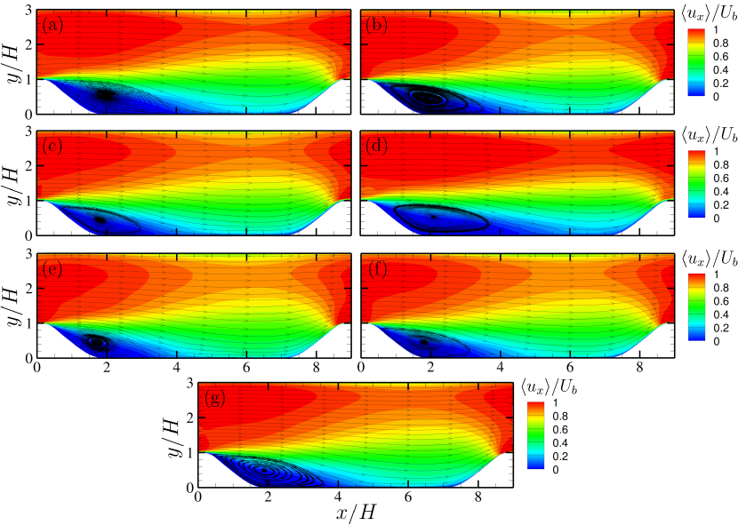
Figure 1: Contours of the mean velocity in $x$ direction and the streamlines at $Re_{H}=10595$ from the simulation cases of (a) RLWM-DSM, (b) RLWM-VRE, (c) RLWM-DSM, coarse mesh, (d) RLWM-VRE, coarse mesh, (e) EQWM-DSM, (f) EQWM-VRE, (g) WRLES [53].

The predictions of the mean skin friction $C_{f}$ and the mean pressure coefficient $C_{p}$ are shown in Fig. 2. The mean skin friction is defined as $C_{f}=\langle\tau_{w}\rangle/(0.5\rho U_{b}^{2})$, where the positive direction of $\tau_{w}$ points toward the opposite direction of bulk flow. The mean pressure coefficient is defined as $C_{p}=(\langle p_{w}\rangle-\langle p^{\text{ref}}\rangle)/(0.5\rho U_{b}^{2})$, where the pressure at $x/H=0$ on the top wall is chosen as reference pressure $p^{\text{ref}}$ [52]. Regarding $C_{f}$, the results from the RLWM simulations are in reasonable agreement with the DNS data, with large deviations found only near the top of the hill on the leeward side where the skin friction rapidly decreases from its maximum value to a negative value. However, the results are better than the EQWM simulations which largely under-predict the skin friction on the windward side of the hill. Furthermore, the mean locations of the separation and reattachment points (listed in Table 2) are better predicted by the RLWMs, consistent with the streamline shown in Fig. 1. All simulations capture the qualitative trend of the mean $C_{p}$ on the bottom wall including the APG and FPG regimes, but large deviations among the simulation cases are visible near the top of the hill ($x/H\geq 8.5$ or $x/H\leq 0.5$) where the pressure sees a sudden change from strong FPG to strong APG and the flow separation emerges. Overall, the RLWMs provide more accurate predictions of $C_{f}$ and $C_{p}$ than the EQWM. When comparing the two developed wall models, it is evident that their predictions differ. Specifically, noticeable variations are seen in the results for $C_{f}$ and $C_{p}$, particularly within the regions of the separation bubble and the windward side of the hill. Additionally, the performance of these models displays a sensitivity to mesh resolution. This sensitivity is evident not only in $C_{f}$ and $C_{p}$ but also in the velocity field, as depicted in Fig. 1. It should be mentioned that the environmental states used for the developed wall models do not contain any information related to the mesh resolution, which could potentially contribute to the sensitivity.

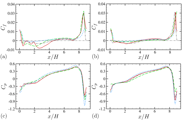
Figure 2: Comparison of (a,b) mean skin friction coefficient and (c,d) mean pressure coefficient along the bottom wall at $Re_{H}=10595$ between the WMLES and the corresponding DNS results [52]. The left column (a,c) presents simulation cases with the DSM, while the right column (b,d) features cases with the Vreman model. Red solid line, RLWM; green dashed line, RLWM with the coarse mesh; blue dashed line, EQWM; black dash-dotted line, DNS [52]; black dash-dot-dotted line, $C_{f}=0$.

Quantitative comparison of mean velocity and Reynolds stress components at five streamwise locations ($x/H=0.05,2,4,6\text{ and }8$) are shown in Fig. 3. The mean velocity and Reynolds stress profiles from the baseline-mesh RLWM simulations align closely with the reference DNS data. However, discrepancies are visible for the locations on the hill where the pressure gradient is strong. The EQWM simulations do not match up as well to the developed wall models, especially regarding the Reynolds stress components. Moreover, the predictions from the coarse-mesh simulations using both RLWM-DSM and RLWM-VRE are less ideal when compared to their baseline-mesh counterparts. It should be mentioned that the prediction of the velocity field not only depends on the wall boundary conditions but also on the SGS model, and the inconsistent results of RLWM simulations across different mesh resolutions may also be influenced by the varying performance of the SGS model in each mesh.

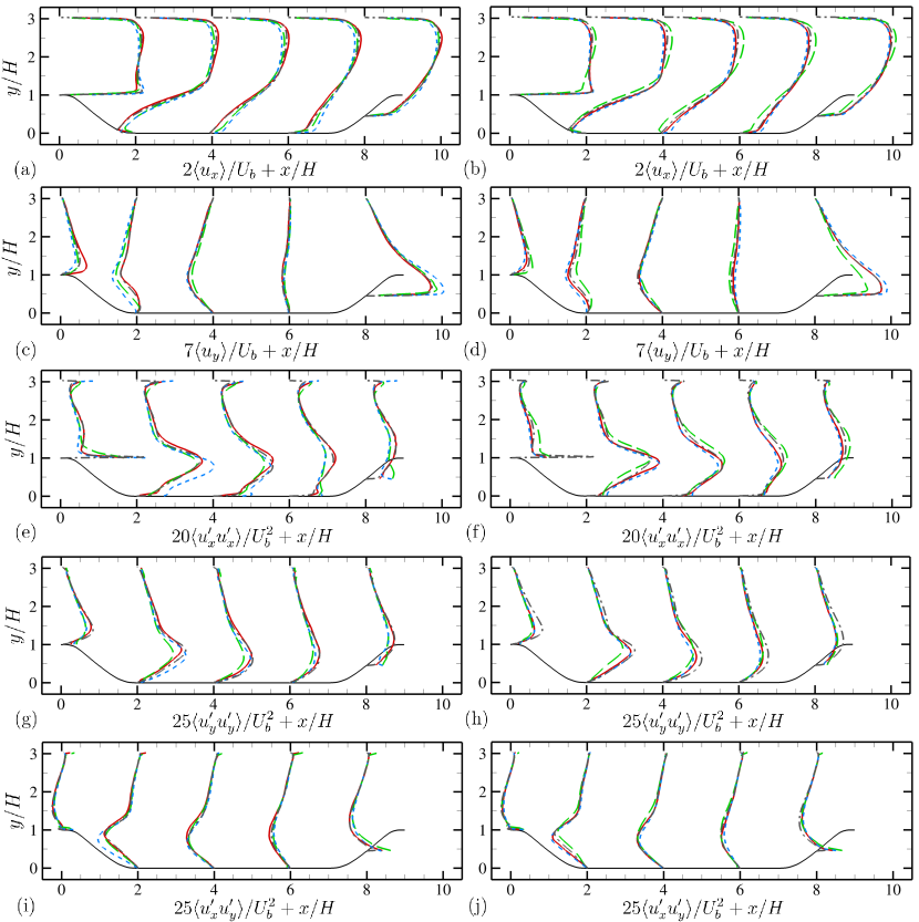
Figure 3: Comparison of mean velocity and Reynolds stress components at $Re_{H}=10595$ between the WMLES and the corresponding DNS results [52]: (a,b) mean streamwise velocity; (c,d) mean vertical velocity; (e,f) streamwise Reynolds stress; (g,h) vertical Reynolds stress; (i,j) Reynolds shear stress. The left column (a,c,e,g,i) presents simulation cases with the DSM, while the right column (b,d,f,h,j) features cases with the Vreman model. Red solid line, RLWM; green dashed line, RLWM with the coarse mesh; blue dashed line, EQWM; black dash-dotted line, DNS [52].

To better understand the mechanism of the trained models, we examine the state-action maps obtained from the baseline-mesh test simulations, which are the probability density functions (PDFs) of the likelihood that the models take a particular action conditioned on the occurrence of positive rewards. Such state-action maps could offer valuable insights that aid the development of empirical models for turbulent flows subjected to various pressure gradients. Figures 4 and 5 show the maps for RLWM-DSM as well as RLWM-VRE based on instantaneous states and actions at three streamwise positions $x/H=0.1,2\text{ and }8.5$ which are located near the top of the hill on its leeward side, within the separation bubble, and the windward side of the hill, respectively. It is worth noting that while rewards are computed for illustrative purposes in this context, they are not employed during the test simulations. Overall, the action contour lines for increasing and decreasing $\nu_{t,w}$ are well separated, which illustrates the models are able to distinguish flow states and provide appropriate actions. In particular, it is evident that RLWM-VRE offers clearer separation in the contour lines of these state-action maps than RLWM-DSM does. This suggests better performance by RLWM-VRE in the baseline-mesh simulations at $Re_{H}=10595$, especially in areas near the top of the hill on its leeward side and within the separation bubble (as seen in Figs. 2 and 3).

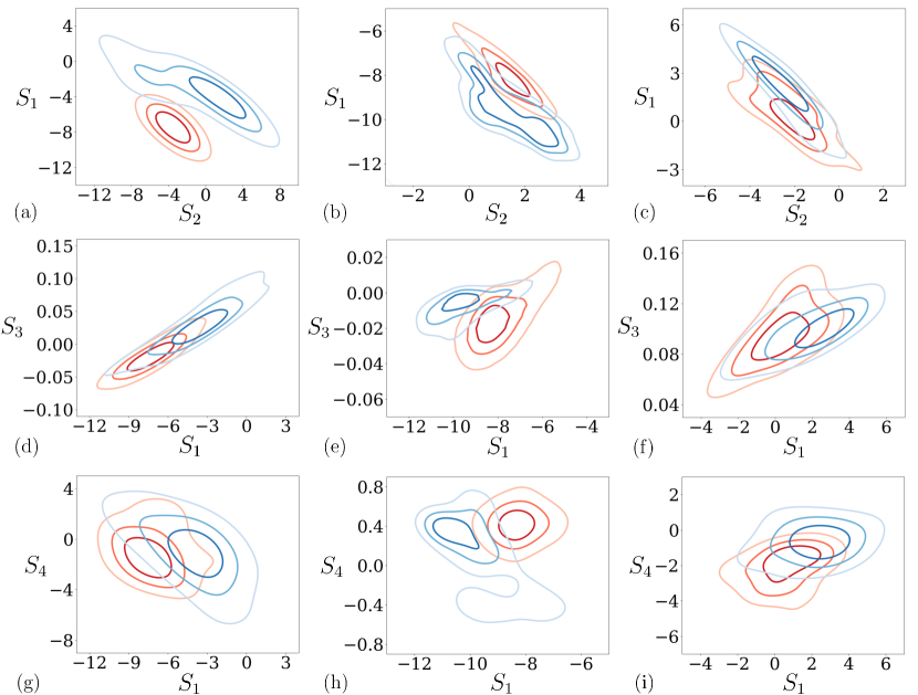
Figure 4: PDFs of states for RLWM-DSM conditioned to events with $r>0.1$ and $a<0.9995$ (blue) or $a>1.0005$ (red) at (a,d,g) $x/H=0.1$, (b,e,h) $x/H=2$ and (c,f,i) $x/H=8.3$ from the baseline-mesh simulation at $Re_{H}=10595$: PDFs of states (a–c) $S_{2}$ and $S_{1}$, (d–f) $S_{1}$ and $S_{3}$ and (g–i) $S_{1}$ and $S_{4}$. Contour levels are $25$, $50$, $75\%$ of the maximum value.

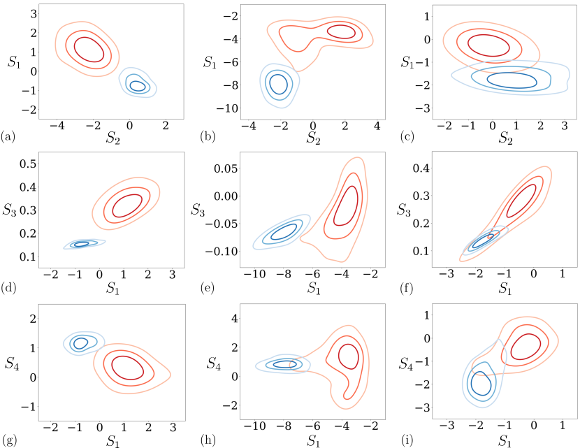
Figure 5: PDFs of states for RLWM-VRE conditioned to events with $r>0.1$ and $a<0.9995$ (blue) or $a>1.0005$ (red) at (a,d,g) $x/H=0.1$, (b,e,h) $x/H=2$ and (c,f,i) $x/H=8.3$ from the baseline-mesh simulation at $Re_{H}=10595$: PDFs of states (a–c) $S_{2}$ and $S_{1}$, (d–f) $S_{1}$ and $S_{3}$ and (g–i) $S_{1}$ and $S_{4}$. Contour levels are $25$, $50$, $75\%$ of the maximum value.

3.2.2 Testing for flow over periodic hills at higher Reynolds numbers

In this section, the RLWMs are applied to WMLES of periodic-hill channel flow at $Re_{H}=19000$ and $37000$. The simulations are conducted by using the baseline mesh ($128\times 64\times 64$) and the coarse mesh ($64\times 32\times 32$), and the implementation of the RLWMs is similar to the simulations at $Re_{H}=10595$. All simulations are run for about 50 FTTs after initial transients. The results from the EQWM with baseline mesh and the WRLES [53] are included for comparison.

The mean skin friction coefficients along the bottom wall at $Re_{H}=19000$ and $37000$ are shown in Fig. 6. The distributions of $C_{f}$ at higher Reynolds numbers have a similar shape as the one shown in Fig. 2(a,b). As the Reynolds number increases, the peak value of the $C_{f}$ on the windward side of the hill decreases. The RLWM simulations align more closely with the WRLES results on hill windward side than the EQWM simulations do. Regarding the separation point, the predicted locations from the RLWM simulations are further downstream than that of the WRLES. Moreover, the RLWMs predict a reattachment location further upstream. Unlike the EQWM simulations, which considerably underestimate the size of the separation bubble, the RLWM simulations are more accurate. Similar to the aforementioned results observed at $Re_{H}=10595$, the RLWM predictions at these higher Reynolds numbers display sensitivity to mesh resolutions.

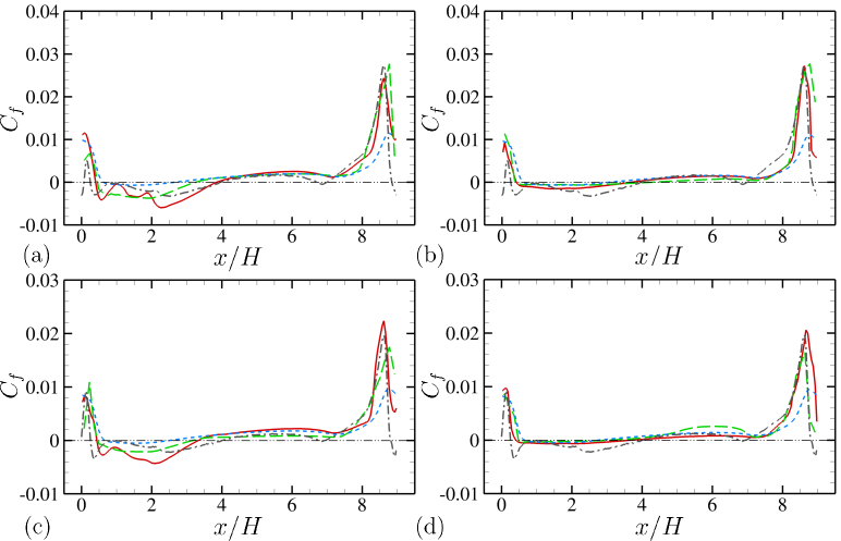
Figure 6: Comparison of mean skin friction coefficient along the bottom wall at (a,b) $Re_{H}=19000$ and (c,d) $Re_{H}=37000$ between the WMLES and the corresponding WRLES results [53]. The left column (a,c) presents simulation cases with the DSM, while the right column (b,d) features cases with the Vreman model. Red solid line, RLWM; green dashed line, RLWM with the coarse mesh; blue dashed line, EQWM; black dash-dotted line, WRLES [53]; black dash-dot-dotted line, $C_{f}=0$.

Figure 7 presents the profiles of the streamwise components for both mean velocity and Reynolds stress at five streamwise stations ($x/H=0.05,2,4,6,\text{ and }8$) for $Re_{H}=19000$ and $37000$. As the Reynolds number increases, the discrepancies between the RLWM simulations and the WRLES profiles become more pronounced, suggesting a diminishing efficacy in the RLWMs. Among the simulations employing the developed wall models, those with RLWM-DSM yield better velocity-field predictions compared to those with RLWM-VRE, especially at $Re_{H}=37000$. Furthermore, when the Reynolds number rises to $Re_{H}=37000$, the EQWM simulations deliver velocity-field results that match or even surpass the RLWM simulations, despite their inaccurate predictions of $C_{f}$, as illustrated in Fig. 6(c,d).

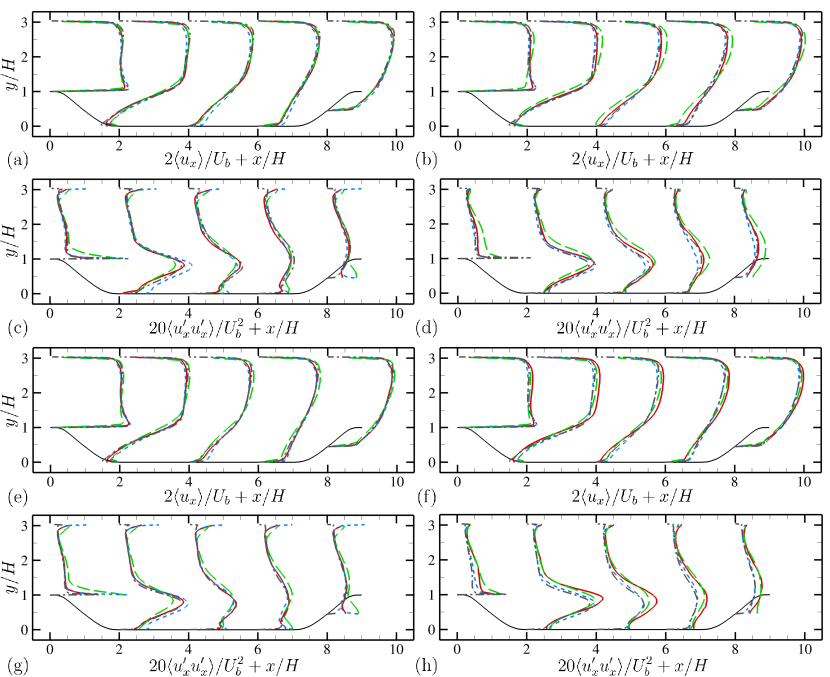
Figure 7: Comparison of (a,b,e,f) mean streamwise velocity and (c,d,g,h) streamwise Reynolds stress at (a,b,c,d) $Re_{H}=19000$ and (e,f,g,h) $Re_{H}=37000$ between the WMLES and the corresponding WRLES results [53]. The left column (a,c,e,g) presents simulation cases with the DSM, while the right column (b,d,f,h) features cases with the Vreman model. Red solid line, RLWM; green dashed line, RLWM with the coarse mesh; blue dashed line, EQWM; black dash-dotted line, WRLES [53].

4 Simulations for Flow over Boeing Gaussian Bump

The geometry of the Boeing Gaussian bump is given by the analytic function

$$y=f(x,z)=\frac{h}{2}e^{-\left(x/x_{0}\right)^{2}}\left\{1+{\rm erf}\left[\left(\frac{L}{2}-2z_{0}-|z|\right)/z_{0}\right]\right\}~{},$$ (3)

where $h=0.085L$, $x_{0}=0.195L$, and $z_{0}=0.06L$. The cross-sections of the bump are shown in Fig. 8. Additionally, the length scale $L$ is used to define the Reynolds number $Re_{L}=U_{\infty}L/\nu$. This geometry has been the subject of extensive experimental research in recent years [26, 27, 28, 29, 30]. The experimental geometry includes side and top walls, as the Gaussian bump is wall-mounted on a splitter plate inside of a wind tunnel. In this work, this geometry with side and top walls is considered. Particularly, the case of $Re_{L}=2\times 10^{6}$ is simulated, and the WMLES results are compared with the experimental measurements.

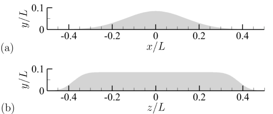
Figure 8: Cross-sections of the Boeing Gaussian bump geometry showing (a) a slice along the centerline ($z/L=0$) and (b) a slice along the span ($x/L=0$).

4.1 Computational details

The present simulations employ a rectangular computational domain with the dimension of $L_{x}\times L_{y}\times L_{z}=2.5L\times 0.5L\times 0.5L$, which has the same blockage ratio as in the wind tunnel experiment [27, 28, 29, 30]. The origin of the coordinate system in the domain locates at the base of the bump peak as shown in Fig. 8. Because symmetry exists with respect to the center plane at $z/L=0$ in the geometry, the simulation domain only covers half of the entire bump span with a symmetry boundary condition applied at $z/L=0$. Besides the developed RLWMs at the bottom wall, we set the simulations with a plug flow inlet at $x/L=-1$. The side at $z/L=0.5$ and top boundary conditions at $y/L=0.5$ are treated as inviscid walls to approximate the wind tunnel condition. The outlet is placed at $x/L=1.5$ with a convective outflow boundary condition. Note that preliminary investigations suggest insensitivity to the inlet and tunnel wall boundary conditions [35, 36].

The simulations are conducted using the aforementioned unstructured-mesh, incompressible, finite-volume flow solver that is coupled with the RL toolbox, smarties [56]. For consistency, both the DSM and the Vreman model, previously utilized in the wall-model training, are adopted in separate simulations. Apart from the developed RLWMs, we employ the EQWM at the bottom wall in the benchmark simulations for comparison, and the center of the second off-wall cell is selected as the matching location in these simulations. Additionally, a maximum CFL number of 2 is used in all simulations.

To study the effect of mesh resolution on the simulation results, three computational meshes with increasing resolutions in each direction are considered. These meshes consist of structured-mesh blocks covering the entire bump surface and the flat wall surfaces in both the upstream and downstream, and unstructured-mesh blocks elsewhere. The wall-normal dimension of the structured-mesh blocks is equal to $0.12L$, which covers the entire TBL on the bottom wall. Furthermore, uniform mesh resolutions are used within the structured-mesh blocks in both streamwise and spanwise directions. Along the wall-normal direction, the mesh size gradually coarsens away from the wall with an approximate stretching ratio of 1.013. Referring to the TBL thickness at $x/L=-0.683$ from the experiment [27, 28, 29, 30], the TBL is approximately resolved by 3 cells in the coarse mesh, 6 cells in the medium mesh, and 9 cells in the fine mesh, respectively. For the unstructured-mesh blocks, the outermost unstructured mesh has the resolution of $0.03L$ and the control volumes are refined gradually towards the bottom wall. More parameters of the computational meshes are provided in Table 3.

In the simulations using the developed RLWMs, the number of agents above the bottom surface is consistent with the number of wall cells in each mesh. The wall-normal matching location of the agents is chosen to be within the first off-wall cell. The wall eddy viscosity $\nu_{t,w}$ is updated at each time step based on the model action. To eliminate numerical artifacts, all simulations are run for 1.5 FTTs at first to pass the transient process. After that, these simulations are run for another 1.5 FTTs to collect flow statistics.

Table 3: Mesh parameters of the simulations for the flow over Boeing Gaussian bump at $Re_{L}=2\times 10^{6}$.

Mesh	$N_{\text{CV}}$	$\min\Delta_{x}/L$	$\min\Delta_{y}/L$	$\min\Delta_{z}/L$
Coarse	$6$ mil.	$3.8\times 10^{-3}$	$2.6\times 10^{-3}$	$2.6\times 10^{-3}$
Medium	$37$ mil.	$1.9\times 10^{-3}$	$1.3\times 10^{-3}$	$1.3\times 10^{-3}$
Fine	$100$ mil.	$1.3\times 10^{-3}$	$9\times 10^{-4}$	$9\times 10^{-4}$

4.2 Results and Discussion

Figure 9 shows contours of the instantaneous streamwise velocity $u_{x}/U_{\infty}$ in an $x$-$y$ plane at $z/L=0$ obtained from the medium-mesh simulations with different wall models and SGS models. The flow gradually accelerates on the windward side of the bump, and the velocity reaches its maximum value at the bump peak. Downstream of the peak, the flow decelerates over the leeward side of the bump, and the boundary layer thickens rapidly. Note that the flow is attached over the entire bump surface in the simulations, which is qualitatively different with the experimental observations that the flow is separated on the leeward side of the bump [26, 27, 28, 29, 30]. Detailed quantitative comparison of mean velocity from different simulations will be discussed later.

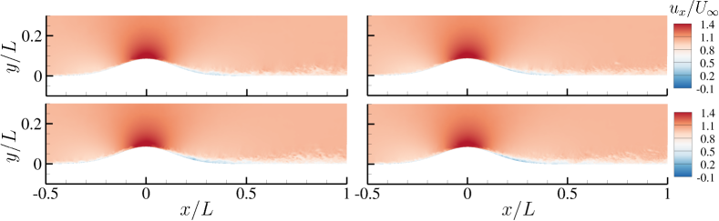
Figure 9: Instantaneous streamwise velocity $u_{x}/U_{\infty}$ in an $x-y$ plane at $z/L=0$ from medium-mesh simulations with RLWM-DSM and DSM (top left), RLWM-VRE and Vreman model (top right), EQWM and DSM (bottom left), and EQWM and Vreman model (bottom right).

Additional quantities of interest for the bump-flow simulations include the mean skin friction coefficient, $C_{f}$, and the mean pressure coefficient, $C_{p}$, which are defined as

$$C_{f}=\frac{\overline{\tau_{w}}}{\frac{1}{2}\rho_{\infty}U_{\infty}^{2}}\qquad\textrm{and}\qquad C_{p}=\frac{\overline{p_{w}}-p_{\infty}}{\frac{1}{2}\rho_{\infty}U_{\infty}^{2}}~{},$$ (4)

respectively. Here, the mean pressure at the inlet near the top boundary is chosen as the reference freestream pressure $p_{\infty}$. Figure 10 presents the distributions of the mean skin friction coefficient $C_{f}$ over the bump surface. For comparison, the data from the experiment using the same geometry at the same Reynolds number from Gray et al. [28] is also shown. Upstream of the bump, the $C_{f}$ results from these simulations exhibit similar trend as the experiments. However, in the experiments, a large separation bubble appears downstream of the bump peak, which is not captured in all simulations. Considering the performance of different wall models, the simulations using the EQWM overpredict $C_{f}$ near the bump peak. However, the developed RLWMs provide more accurate predictions for this region, and as the mesh resolutions increase, the predictions of $C_{f}$ are consistent and agree well with the experimental data. While the performance of the current RLWMs within the region upstream of the bump is better than that of the EQWM, it is still suboptimal. This is expected as the model training does not encompass laminar or transitional flows. On the leeward side of the bump, the predictions of $C_{f}$ from both wall models are comparable. However, further downstream, the developed RLWMs provide lower skin friction than the EQWM.

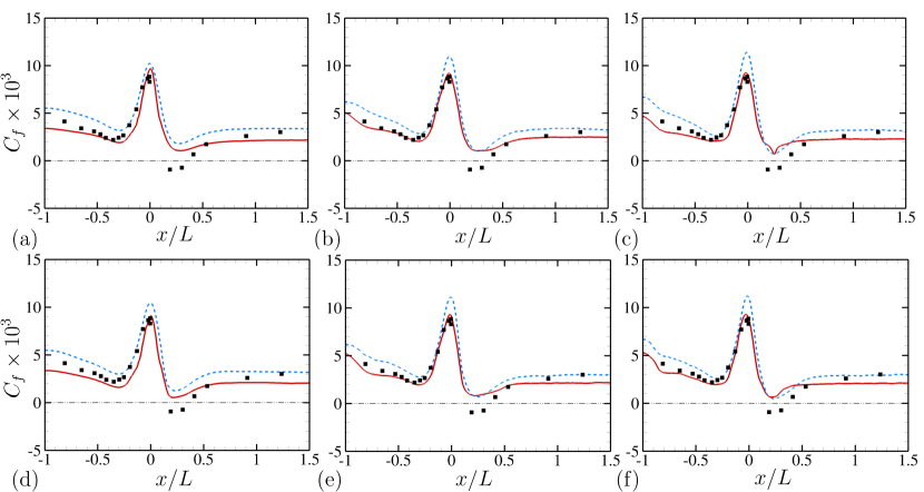
Figure 10: The distributions of mean skin friction coefficient along the bump surface at $z/L=0$ from the simulations with (a,d) coarse mesh, (b,e) medium mesh and (c,f) fine mesh. The top row presents simulation cases using the DSM, while the bottom row features cases using the Vreman model. Red solid line, RLWM; blue dashed line, EQWM; black dash-dot-dotted line, $C_{f}=0$; squares, experimental measurements at $Re_{L}=2\times 10^{6}$ [28].

Figure 11 shows the distribution of $C_{p}$ along the bump surface at $z/L=0$. Results from all simulations with different computational meshes are included along with the experimental measurements of Gray et al. [28] at the same Reynolds number. The $C_{p}$ distributions illustrate strong FPG immediately upstream of the bump peak. Downstream of the peak, the flow is first subjected to a very strong APG then followed by a mild FPG. Comparison of simulation results with experimental data reveals significant differences on the leeward side of the bump, which is expected due to the imprecise capture of the separation bubble in the simulations. Furthermore, the variations in mesh resolution do not significantly affect $C_{p}$ predictions in these simulations. In terms of wall model performance, the RLWMs and EQWM provide similar $C_{p}$ predictions, with only minor differences observed on the leeward side of the bump. In addition, when examining the $C_{p}$ distributions along the span, the simulation results align closely with each other and with the experimental data in the outer-span region ($z/L>0.2$). However, discrepancies become noticeable near the center of the bump, where a downstream separation bubble is expected. For brevity, detailed results are omitted here but can be found in [39].

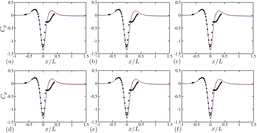
Figure 11: The distributions of mean pressure coefficient along the bump surface at $z/L=0$ from the simulations with (a,d) coarse mesh, (b,e) medium mesh and (c,f) fine mesh. The top row presents simulation cases using the DSM, while the bottom row features cases using the Vreman model. Red solid line, RLWM; blue dashed line, EQWM; squares, experimental measurements at $Re_{L}=2\times 10^{6}$ [28].

In Fig. 12, profiles of the mean streamwise velocity are depicted at four streamwise stations $x/L=-0.4,-0.1,0.1$ and 0.2, which are located within the regions with mild APG, strong FPG, and strong APG, respectively. These results quantitatively show the flow acceleration as well as deceleration and boundary-layer thickening on the bump surface. Based on the comparison in the figure, the simulation results downstream of the bump exhibit significant differences from the experiment conducted by Gray et al. [29], with the simulations predicting a thinner TBL. This finding is consistent with the earlier observation of the instantaneous flow field. The simulations employing the two different RLWMs display significant differences at $x/L=-0.1$ where the FPG is pronounced. However, for most other locations, the results from both simulations align closely. When examining the EQWM simulations, velocity predictions exhibit small variation across different SGS models, and these predictions are comparable to those from the RLWM simulations on the leeward side of the bump. Nevertheless, at $x/L=-0.4$, the EQWM outperforms the RLWMs in velocity prediction, even though its prediction of mean skin friction is less ideal, as illustrated in Fig. 10.

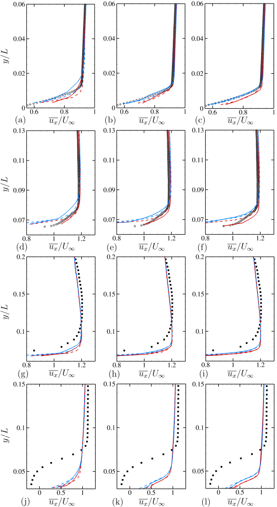
Figure 12: Profiles of mean velocity $\overline{u_{x}}/U_{\infty}$ on an $x-y$ plane of $z/L=0$ at (a,b,c) $x/L=-0.4$, (d,e,f) $x/L=-0.1$, (g,h,i) $x/L=0.1$, and (j,k,l) $x/L=0.2$ from the simulations with coarse mesh (left), medium mesh (center), and fine mesh (right). Solid lines indicate simulations using the DSM, and dashed lines indicate simulations using the Vreman model. Red lines denote the simulations with the RLWMs, and blue lines denote the simulations with the EQWM. Squares and circles represent Particle Image Velocimetry (PIV) and Stereoscopic PIV (SPIV) measurements at $Re_{L}=2\times 10^{6}$ [29], respectively.

While data-driven turbulence models often have limited applicability across different flow configurations [61], the current RLWMs, originally trained on the low-Reynolds-number periodic-hill channel flow, show promise in simulating the flow over the Boeing Gaussian bump, which has a different geometry as well as higher Reynolds number and is likely to exhibit different flow physics. Specifically, the RLWMs provide improved predictions for the skin friction near the peak of the bump and perform comparably to the EQWM with respect to the wall pressure and velocity field. For the sake of consistency, the SGS models used in the present bump-flow RLWM simulations correspond to those employed during model training. However, there is no strict requirement to utilize the same SGS model. In fact, previous simulations by Zhou et al. [39], which combined RLWM-DSM with the anisotropic minimum-dissipation SGS model [62], yielded improved predictions for the flow. In addition, a sensitivity analysis of WMLES by Zhou and Bae [45] highlighted the significant impact of SGS models on separated flow simulations. Specifically, this study revealed that the influence of wall boundary conditions on predicting separation bubble is overshadowed by that of the SGS models. Thus, the inability to capture separation in all the bump-flow simulations from this study can be largely attributed to the SGS models.

5 Summary

Using multi-agent reinforcement learning, we develop two wall models capable of adapting to various pressure-gradient effects. These models are trained based on LES of low-Reynolds-number periodic-hill channel flow, each incorporating a different SGS model. Both models function as control policies for wall eddy viscosity, aiming to predict the correct wall-shear stress. During the training process, the optimized policy for each wall model is learned from LES with cooperating agents using the recovery of the correct wall-shear stress as a reward. The developed wall models are first validated in the LES of the periodic-hill configuration at the same Reynolds number of model training. The wall models provide good predictions of mean wall-shear stress, mean wall pressure, and the mean velocity as well as Reynolds stress in the flow field. The test results also show that the developed models outperform the EQWM. The performance of the developed models is further evaluated at two higher Reynolds numbers ($Re_{H}=19000$ and $37000$). Good predictions are obtained for the mean wall-shear stress and velocity statistics.

To further investigate the applicability and robustness of the developed wall models, simulations of flow over the Boeing Gaussian bump at a moderately high Reynolds number are conducted. The flow geometry is consistent with the experiments [27, 28, 29, 30], and the Reynolds number based on the freestream velocity and the width of the bump is $2\times 10^{6}$. The results of mean skin friction and pressure on the bump surface and the velocity statistics of the flow field are compared to those from the EQWM simulations and published experimental data sets. It shows that the developed wall models successfully capture the acceleration and deceleration of the TBL on the bump surface. In addition, these models offer more accurate predictions of skin friction around the peak of the bump, and their performance in predicting wall pressure and the velocity field is comparable to that of the EQWM.

On the foundation of the test simulations across various flow configurations, it is evident that the RLWMs in this study, developed based on the training with low-Reynolds-number periodic-hill channel flow, have gained valuable insights into the key physics of complex flows with diverse pressure gradients. Moreover, this study underscores the promise of the multi-agent reinforcement learning framework in sophisticated turbulence modeling. Further improvements may arise from training these wall models across a broader spectrum of Reynolds numbers and flow geometries using the framework. However, it is clear from the test simulations that the developed models display sensitivity to mesh resolutions. This sensitivity might be mitigated by incorporating the mesh parameter into RL-based wall model as an environmental state. The role of SGS models in shaping the wall model development is also discernible, especially given their significant influence in simulations of separated turbulent flow [45]. To improve the reliability and versatility of RL-based wall model in wider applications, a potential avenue worth exploring is extending the wall model to become a unified model that encompasses both SGS and wall boundary modeling, as seen in models like the building-block flow model [14, 15, 16].

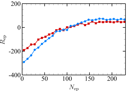
Figure 13: Averaged episode reward $R_{\text{ep}}$ against episode number $N_{\text{ep}}$ during the training of RLWMs. Red line with squares, RLWM-DSM; blue line with circles, RLWM-VRE.

Appendix: Convergence of Model Training

As detailed in Section 3.1.3, the training of models is based on a series of periodic-hill channel flow simulations. In order to accelerate the training, 8 simulations (episodes) run in parallel. Subsequently, the policies of the trained models are updated after every set of 8 episodes, defining one iteration. Figure 13 shows the averaged episode rewards $R_{\text{ep}}$ for all iterations during the training of the aforementioned two RLWMs with different SGS models. The averaged episode reward for each iteration is defined as $R_{\text{ep}}=(1/8)\sum_{l=1}^{8}\sum_{k=1}^{N_{\text{k}}}\sum_{j=1}^{N_{j}}r_{j,k,l}$, where $j$ denotes the $j$-th sampling step in one episode, $N_{j}$ represents the total number of sampling steps in one episode, $k$ denotes the index of RL agent, $N_{k}$ is the total count of RL agents in each episode and $l$ marks the index of episode in one iteration. From the presented results, it is evident that the training converges around 200 episodes or 25 iterations for both cases.

References

- Balaras et al. [1996] Balaras, E., Benocci, C., and Piomelli, U., “Two-Layer Approximate Boundary Conditions for Large-Eddy Simulations,” AIAA Journal, Vol. 34, No. 6, 1996, pp. 1111–1119. 10.2514/3.13200.
- Piomelli and Balaras [2002] Piomelli, U., and Balaras, E., “Wall-Layer Models for Large-Eddy Simulations,” Annual Review of Fluid Mechanics, Vol. 34, No. 1, 2002, pp. 349–374. 10.1146/annurev.fluid.34.082901.144919.
- Wang and Moin [2002] Wang, M., and Moin, P., “Dynamic Wall Modeling for Large-Eddy Simulation of Complex Turbulent Flows,” Physics of Fluids, Vol. 14, No. 7, 2002, pp. 2043–2051. 10.1063/1.1476668.
- Chung and Pullin [2009] Chung, D., and Pullin, D. I., “Large-Eddy Simulation and Wall Modelling of Turbulent Channel Flow,” Journal of Fluid Mechanics, Vol. 631, 2009, pp. 281–309. 10.1017/S0022112009006867.
- Park and Moin [2014] Park, G. I., and Moin, P., “An Improved Dynamic Non-Equilibrium Wall-Model for Large Eddy Simulation,” Physics of Fluids, Vol. 26, No. 1, 2014, pp. 37–48. 10.1063/1.4861069.
- Larsson et al. [2016] Larsson, J., Kawai, S., Bodart, J., and Bermejo-Moreno, I., “Large Eddy Simulation with Modeled Wall-Stress: Recent Progress and Future Directions,” Mechanical Engineering Reviews, Vol. 3, No. 1, 2016, pp. 15–00418. 10.1299/mer.15-00418.
- Bose and Park [2018] Bose, S. T., and Park, G. I., “Wall-Modeled Large-Eddy Simulation for Complex Turbulent Flows,” Annual Review of Fluid Mechanics, Vol. 50, 2018, pp. 535–561. 10.1146/annurev-fluid-122316-045241.
- Bose and Moin [2014] Bose, S. T., and Moin, P., “A Dynamic Slip Boundary Condition for Wall-Modeled Large-Eddy Simulation,” Physics of Fluids, Vol. 26, No. 1, 2014, p. 015104. 10.1063/1.4849535.
- Bae et al. [2019] Bae, H. J., Lozano-Durán, A., Bose, S. T., and Moin, P., “Dynamic Slip Wall Model for Large-Eddy Simulation,” Journal of Fluid Mechanics, Vol. 859, 2019, pp. 400–432. 10.1017/jfm.2018.838.
- Zhou et al. [2021] Zhou, Z., He, G., and Yang, X., “Wall Model Based on Neural Networks for LES of Turbulent Flows over Periodic Hills,” Physical Review Fluids, Vol. 6, No. 5, 2021, p. 054610. 10.1103/PhysRevFluids.6.054610.
- Zhou et al. [2023] Zhou, Z., Yang, X. I., Zhang, F., and Yang, X., “A Wall Model Learned from the Periodic Hill Data and the Law of the Wall,” Physics of Fluids, Vol. 35, No. 5, 2023. 10.1063/5.0143650.
- Vadrot et al. [2023a] Vadrot, A., Yang, X. I., and Abkar, M., “Survey of Machine-Learning Wall Models for Large-Eddy Simulation,” Physical Review Fluids, Vol. 8, No. 6, 2023a, p. 064603. 10.1103/PhysRevFluids.8.064603.
- Lozano-Durán and Bae [2023] Lozano-Durán, A., and Bae, H. J., “Machine Learning Building-Block-Flow Wall Model for Large-Eddy Simulation,” Journal of Fluid Mechanics, Vol. 963, 2023, p. A35. 10.1017/jfm.2023.331.
- Ling et al. [2022] Ling, Y., Arranz, G., Williams, E., Goc, K., Griffin, K., and Lozano-Durán, A., “Wall-Modeled Large-Eddy Simulation Based on Building-Block Flows,” Proceedings of the CTR Summer Program 2022, Center for Turbulence Research, Stanford Univ., Stanford, CA, 2022, pp. 5–14.
- Arranz et al. [June 2023] Arranz, G., Ling, Y., and Lozano-Duran, A., “Wall-Modeled LES Based on Building-Block Flows: Application to the Gaussian Bump,” AIAA Paper 2023–3984, June 2023. 10.2514/6.2023-3984.
- Lozano-Duran et al. [June 2023] Lozano-Duran, A., Arranz, G., and Ling, Y., “Building-Block-Flow Model for Large-Eddy Simulation: Application to NASA CRM-HL,” AIAA Paper 2023–3425, June 2023. 10.2514/6.2023-3425.
- Bertsekas [2019] Bertsekas, D. P., Reinforcement Learning and Optimal Control, Athena Scientific, Nashua, NH, USA, 2019.
- Gazzola et al. [2014] Gazzola, M., Hejazialhosseini, B., and Koumoutsakos, P., “Reinforcement Learning and Wavelet Adapted Vortex Methods for Simulations of Self-Propelled Swimmers,” SIAM Journal on Scientific Computing, Vol. 36, No. 3, 2014, pp. B622–B639. 10.1137/130943078.
- Novati et al. [2017] Novati, G., Verma, S., Alexeev, D., Rossinelli, D., Van Rees, W. M., and Koumoutsakos, P., “Synchronisation Through Learning for Two Self-Propelled Swimmers,” Bioinspiration & biomimetics, Vol. 12, 2017, p. 036001. 10.1088/1748-3190/aa6311.
- Novati et al. [2021] Novati, G., de Laroussilhe, H. L., and Koumoutsakos, P., “Automating Turbulence Modelling by Multi-Agent Reinforcement Learning,” Nature Machine Intelligence, Vol. 3, 2021, pp. 87–96. 10.1038/s42256-020-00272-0.
- Bae and Koumoutsakos [2022] Bae, H. J., and Koumoutsakos, P., “Scientific Multi-Agent Reinforcement Learning for Wall-Models of Turbulent Flows,” Nature Communications, Vol. 13, 2022, pp. 1–9. 10.1038/s41467-022-28957-7.
- Vadrot et al. [2023b] Vadrot, A., Yang, X. I., Bae, H. J., and Abkar, M., “Log-Law Recovery through Reinforcement-Learning Wall Model for Large Eddy Simulation,” Physics of Fluids, Vol. 35, No. 5, 2023b. 10.1063/5.0147570.
- Cabot and Moin [2000] Cabot, W., and Moin, P., “Approximate Wall Boundary Conditions in the Large-Eddy Simulation of High Reynolds Number Flow,” Flow, Turbulence and Combustion, Vol. 63, 2000, pp. 269–291. 10.1023/A:1009958917113.
- Kawai and Larsson [2012] Kawai, S., and Larsson, J., “Wall-Modeling in Large Eddy Simulation: Length Scales, Grid Resolution, and Accuracy,” Physics of Fluids, Vol. 24, No. 1, 2012, p. 015105. 10.1063/1.3678331.
- Slotnick [October 2019] Slotnick, J. P., “Integrated CFD Validation Experiments for Prediction of Turbulent Separated Flows for Subsonic Transport Aircraft,” Separated Flow: Prediction, Measurement and Assessment for Air and Sea Vehicles, STO Publication STO-MP-AVT-307-06, October 2019.
- Williams et al. [January 2020] Williams, O., Samuell, M., Sarwas, E. S., Robbins, M., and Ferrante, A., “Experimental Study of a CFD Validation Test Case for Turbulent Separated Flows,” AIAA Paper 2020–0092, January 2020. 10.2514/6.2020-0092.
- Gray et al. [August 2021] Gray, P. D., Gluzman, I., Thomas, F., Corke, T., Lakebrink, M., and Mejia, K., “A New Validation Experiment for Smooth-Body Separation,” AIAA Paper 2021–2810, August 2021. 10.2514/6.2021-2810.
- Gray et al. [January 2022] Gray, P. D., Gluzman, I., Thomas, F. O., and Corke, T. C., “Experimental Characterization of Smooth Body Flow Separation over Wall-Mounted Gaussian Bump,” AIAA Paper 2022–1209, January 2022. 10.2514/6.2022-1209.
- Gray et al. [June 2022] Gray, P. D., Gluzman, I., Thomas, F. O., Corke, T. C., Lakebrink, M. T., and Mejia, K., “Benchmark Characterization of Separated Flow over Smooth Gaussian Bump,” AIAA Paper 2022–3342, June 2022. 10.2514/6.2022-3342.
- Gluzman et al. [2022] Gluzman, I., Gray, P., Mejia, K., Corke, T. C., and Thomas, F. O., “A Simplified Photogrammetry Procedure in Oil-Film Interferometry for Accurate Skin-Friction Measurement over Arbitrary Geometries,” Experiments in Fluids, Vol. 63, No. 7, 2022, pp. 1–14. 10.1007/s00348-022-03466-x.
- Balin and Jansen [2021] Balin, R., and Jansen, K. E., “Direct Numerical Simulation of a Turbulent Boundary Layer over a Bump with Strong Pressure Gradients,” Journal of Fluid Mechanics, Vol. 918, 2021. 10.1017/jfm.2021.312.
- Wright et al. [January 2021] Wright, J. R., Balin, R., Jansen, K. E., and Evans, J. A., “Unstructured LES_DNS of a Turbulent Boundary Layer over a Gaussian Bump,” AIAA Paper 2021–1746, January 2021. 10.2514/6.2021-1746.
- Uzun and Malik [2022] Uzun, A., and Malik, M. R., “High-Fidelity Simulation of Turbulent Flow past Gaussian Bump,” AIAA Journal, Vol. 60, No. 4, 2022, pp. 2130–2149. 10.2514/1.J060760.
- Iyer and Malik [January 2021] Iyer, P. S., and Malik, M. R., “Wall-Modeled LES of Flow over a Gaussian Bump,” AIAA Paper 2021–1438, January 2021. 10.2514/6.2021-1438.
- Whitmore et al. [2021] Whitmore, M. P., Griffin, K. P., Bose, S. T., and Moin, P., “Large-Eddy Simulation of a Gaussian Bump with Slip-Wall Boundary Conditions,” Annual Research Briefs 2021, Center for Turbulence Research, Stanford Univ., Stanford, CA, 2021, pp. 45–58.
- Agrawal et al. [2022] Agrawal, R., Whitmore, M. P., Griffin, K. P., Bose, S. T., and Moin, P., “Non-Boussinesq Subgrid-Scale Model with Dynamic Tensorial Coefficients,” Physical Review Fluids, Vol. 7, No. 7, 2022, p. 074602. 10.1103/PhysRevFluids.7.074602.
- Balin et al. [June 2020] Balin, R., Jansen, K. E., and Spalart, P. R., “Wall-Modeled LES of Flow over a Gaussian Bump with Strong Pressure Gradients and Separation,” AIAA Paper 2020–3012, June 2020. 10.2514/6.2020-3012.
- Zhou et al. [2022] Zhou, D., Whitmore, M. P., Griffin, K. P., and Bae, H. J., “Multi-Agent Reinforcement Learning for Wall Modeling in LES of Flow over Periodic Hills,” Proceedings of the CTR Summer Program 2022, Center for Turbulence Research, Stanford Univ., Stanford, CA, 2022, pp. 25–34.
- Zhou et al. [June 2023] Zhou, D., Whitmore, M. P., Griffin, K. P., and Bae, H. J., “Large-Eddy Simulation of Flow over Boeing Gaussian Bump Using Multi-Agent Reinforcement Learning Wall Model,” AIAA Paper 2023–3985, June 2023. 10.2514/6.2023-3985.
- You et al. [2008] You, D., Ham, F., and Moin, P., “Discrete Conservation Principles in Large-Eddy Simulation with Application to Separation Control over an Airfoil,” Physics of Fluids, Vol. 20, 2008, p. 101515. 10.1063/1.3006077.
- Van der Vorst [1992] Van der Vorst, H. A., “Bi-CGSTAB: A Fast and Smoothly Converging Variant of Bi-CG for the Solution of Nonsymmetric Linear Systems,” SIAM Journal on scientific and Statistical Computing, Vol. 13, 1992, pp. 631–644. 10.1137/0913035.
- Germano et al. [1991] Germano, M., Piomelli, U., Moin, P., and Cabot, W. H., “A Dynamic Subgrid-Scale Eddy Viscosity Model,” Physics of Fluids A: Fluid Dynamics, Vol. 3, 1991, pp. 1760–1765. 10.1063/1.857955.
- Lilly [1992] Lilly, D. K., “A Proposed Modification of the Germano Subgrid-Scale Closure Method,” Physics of Fluids A: Fluid Dynamics, Vol. 4, 1992, pp. 633–635. 10.1063/1.858280.
- Vreman [2004] Vreman, A. W., “An Eddy-Viscosity Subgrid-Scale Model for Turbulent Shear Flow: Algebraic Theory and Applications,” Physics of Fluids, Vol. 16, No. 10, 2004, pp. 3670–3681. 10.1063/1.1785131.
- Zhou and Bae [2023] Zhou, D., and Bae, H. J., “Sensitivity Analysis of Wall-Modeled Large-Eddy Simulation for Separated Turbulent Flow,” arXiv preprint arXiv:2309.13555, 2023. 10.48550/arXiv.2309.13555.
- Yang and Wang [2013] Yang, Q., and Wang, M., “Boundary-Layer Noise Induced by Arrays of Roughness Elements,” Journal of Fluid Mechanics, Vol. 727, 2013, pp. 282–317. 10.1017/jfm.2013.190.
- Zhou et al. [June 2020] Zhou, D., Wang, K., and Wang, M., “Large-Eddy Simulation of an Axisymmetric Boundary Layer on a Body of Revolution,” AIAA Paper 2020–2989, June 2020. 10.2514/6.2020-2989.
- Zhou et al. [June 2022] Zhou, D., Wang, K., and Wang, M., “Computational Analysis of Noise Generation by a Rotor at the Rear of an Axisymmetric Body of Revolution,” AIAA Paper 2022–3090, June 2022. 10.2514/6.2022-3090.
- Mellen et al. [2000] Mellen, C. P., Fröhlich, J., and Rodi, W., “Large Eddy Simulation of the Flow over Periodic Hills,” Proceedings of the 16th IMACS world congress, Lausanne, Switzerland, 2000, pp. 21–25.
- Fröhlich et al. [2005] Fröhlich, J., Mellen, C. P., Rodi, W., Temmerman, L., and Leschziner, M. A., “Highly Resolved Large-Eddy Simulation of Separated Flow in a Channel With Streamwise Periodic Constrictions,” Journal of Fluid Mechanics, Vol. 526, 2005, pp. 19–66. 10.1017/S0022112004002812.
- Rapp and Manhart [2011] Rapp, C., and Manhart, M., “Flow over Periodic Hills: An Experimental Study,” Experiments in Fluids, Vol. 51, No. 1, 2011, pp. 247–269. 10.1007/s00348-011-1045-y.
- Krank et al. [2018] Krank, B., Kronbichler, M., and Wall, W. A., “Direct Numerical Simulation of Flow over Periodic Hills up to ,” Flow, Turbulence and Combustion, Vol. 101, 2018, pp. 521–551. 10.1007/s10494-018-9941-3.
- Gloerfelt and Cinnella [2019] Gloerfelt, X., and Cinnella, P., “Large Eddy Simulation Requirements for the Flow over Periodic Hills,” Flow, Turbulence and Combustion, Vol. 103, 2019, pp. 55–91. 10.1007/s10494-018-0005-5.
- Xiao et al. [2020] Xiao, H., Wu, J.-L., Laizet, S., and Duan, L., “Flows over Periodic Hills of Parameterized Geometries: A Dataset for Data-Driven Turbulence Modeling from Direct Simulations,” Computers & Fluids, Vol. 200, 2020, p. 104431. 10.1016/j.compfluid.2020.104431.
- Balakumar et al. [2014] Balakumar, P., Park, G. I., and Pierce, B., “DNS, LES, and Wall-Modeled LES of Separating Flow over Periodic Hills,” Proceedings of the CTR Summer Program 2014, Center for Turbulence Research, Stanford Univ., Stanford, CA, 2014, pp. 407–415.
- Novati and Koumoutsakos [2019] Novati, G., and Koumoutsakos, P., “Remember and Forget for Experience Replay,” Proceedings of the 36th International Conference on Machine Learning, PMLR, Long Beach, CA, 2019, pp. 4851–4860.
- Manhart et al. [2008] Manhart, M., Peller, N., and Brun, C., “Near-Wall Scaling for Turbulent Boundary Layers with Adverse Pressure Gradient: A Priori Tests on DNS of Channel Flow with Periodic Hill Constrictions and DNS of Separating Boundary Layer,” Theoretical and Computational Fluid Dynamics, Vol. 22, 2008, pp. 243–260. 10.1007/s00162-007-0055-0.
- Bae and Lozano-Durán [2021] Bae, H. J., and Lozano-Durán, A., “Effect of Wall Boundary Conditions on a Wall-Modeled Large-Eddy Simulation in a Finite-Difference Framework,” Fluids, Vol. 6, 2021, p. 112. 10.3390/fluids6030112.
- Lozano-Durán and Bae [2019] Lozano-Durán, A., and Bae, H. J., “Error Scaling of Large-Eddy Simulation in the Outer Region of Wall-Bounded Turbulence,” Journal of Computational Physics, Vol. 392, 2019, pp. 532–555. 10.1016/j.jcp.2019.04.063.
- Iyer and Malik [2022] Iyer, P. S., and Malik, M. R., “Wall-Modeled LES of Turbulent Flow over a Two Dimensional Gaussian Bump,” ICCFD11-2022-0204, 2022.
- Duraisamy et al. [2019] Duraisamy, K., Iaccarino, G., and Xiao, H., “Turbulence Modeling in the Age of Data,” Annual Review of Fluid Mechanics, Vol. 51, 2019, pp. 357–377. 10.1146/annurev-fluid-010518-040547.
- Rozema et al. [2015] Rozema, W., Bae, H. J., Moin, P., and Verstappen, R., “Minimum-Dissipation Models for Large-Eddy Simulation,” Physics of Fluids, Vol. 27, No. 8, 2015, p. 085107. 10.1063/1.4928700.