Market Making and Pricing of Financial Derivatives based on Road Travel Time

Abstract

Travel time derivatives are financial instruments that derive their value from road travel times, serving as an underlying asset that cannot be directly traded. Within the transportation domain, these derivatives are proposed as a more comprehensive approach to value pricing. They enable road pricing based not only on the level of travel time but also its volatility. In the financial market, travel time derivatives are introduced as innovative hedging instruments to mitigate market risk, particularly in light of recent stress experienced by the crypto market and traditional banking sector.

The paper focuses on three main aspects: (1) the motivation behind the introduction of these derivatives, driven by the demand for hedging; (2) exploring the potential market for these instruments; and (3) delving into the product design and pricing schemes associated with them. The pricing schemes are devised by utilizing real-time travel time data captured by sensors. These data are modeled using Ornstein-Uhlenbeck processes and, more broadly, continuous time autoregressive moving average (CARMA) models. The calibration of these models is achieved through a hidden factor model, which describes the dynamics of travel time processes. The risk-neutral pricing principle is then employed to determine the prices of the derivatives, employing well-designed procedures to identify the market value of risk.

0.1 Keywords

Travel time derivatives, non-tradable asset, financial derivatives, asset pricing, travel time forecast, time series, CARMA process, hidden factor models.

1 Initiation and necessity analysis

This paper introduces the concept of a travel time derivative as an alternative approach to congestion pricing, sometimes referred to as value pricing, for use by transportation facilities. A travel time derivative is a useful financial product to (a) hedge against transportation-related risk by users of the transportation facility, (b) manage the demand for those facilities through derivatives-based dynamic tolling, (c) contribute to risk mitigation through portfolio diversification and (d) provide an additional source of revenue for owners of transportation facilities. In this paper, potential market participants are analyzed first, and then major products designed for a travel time derivatives market are presented. Alternative models for describing underlying travel time changes are discussed, together with corresponding pricing methods.

1.1 Derivatives and weather derivatives as hedging tools

Derivatives are financial instruments whose prices are derived from the value of something else, known as the underlying asset. The major types of derivatives are forwards, futures, options, and swaps [1]. Any stochastic changing element that generates changes in cash flow can serve as the underlying asset. Therefore, the underlying element upon which a derivative is based can be the price of an asset (e.g., commodities, equities [stock], residential mortgages, commercial real estate, loans, bonds), the value of an index (e.g., interest rates, exchange rates, stock market indices, consumer price index [CPI]), or other items (e.g., temperature, precipitation). The underlying elements of derivatives can be further classified as tradable and non-tradable. Most items listed in the preceding paragraph as bases for derivatives can be traded in a market and so are called tradable underlying assets. A few others, such as temperature, precipitation, and travel time, are non-tradable. This difference in the tradability of an underlying asset triggers differences in market making mechanism, trading strategy and pricing methods.

Derivatives based on non-tradable assets were first introduced in 1999, when the Chicago Mercantile Exchange introduced weather futures contracts, the payoffs for which are based on average temperatures at specified locations. According to [2], weather derivatives offer an innovative hedging instrument to firms facing the possibility of significant earnings declines or advances because of unpredictable weather patterns. [3] analyzed participants and roles in that futures market and found that weather derivatives act as alternative and more flexible ways of insuring against weather related risk. Industries subject to weather risk participate in the buy/sell side of the market, while speculators, who trade purely for profit, provide an important source of liquidity.

Weather derivatives provide insurance to farmers and agriculture companies against bad weather and low crop output. The payoff for one farmer who grows corn and buys a weather derivative contract is as follows: When the weather is good, the insured benefits from abundant corn output; when the weather is bad, the insured receives extra compensation from the derivative to cover losses in corn sales. In this way, the insured hedges risk. This risk-protection mechanism is shown in Table 1. In the table, $G$ represents the gain on the derivative, and $P$ represents the premium that the farmer pays for the contract.

Table 1: Payoff of typical weather derivatives

Weather Condition	Corn production payoff	Derivative payoff
Good	$G_{good}$	$-P$
Bad	$G_{bad}$	$G-P$

As weather derivatives are used to hedge risk related to temperature, precipitation, and other factors, the pricing of weather derivatives should primarily be based upon prediction of weather conditions. Based on accurate prediction of future weather changes, the contract is priced using different methods other than the Black-Scholes pricing model, considering the fact that weather conditions are not traded in the market. These pricing methods are not founded on dynamic hedging of the un-tradable underlying instruments but on other more general pricing schemes such as risk neutral pricing under incomplete market conditions, indifferent pricing principles and etc, which are introduced in greater detail in later sections.

1.2 Road pricing for changing traffic patterns and generating revenue

The concept of using road tolls as a means of reducing traffic congestion was first introduced by economist Arthur Pigou [4]. Tolls can serve as a revenue generator for road infrastructure financing, or as a transportation management tool to curb peak hour travel and related traffic congestion. A considerable amount of literature exists on the methodology of road tolls, and several studies are reviewed in this section.

Vovsha (2006) [5] explored a wide range of possible modeling techniques for road pricing, from simplified sketch-planning tools for short-term revenue forecasting to comprehensive travel demand models for large-scale problems. The study emphasized models associated with advanced network simulation tools, such as dynamic traffic assignment and microsimulation, and advanced activity-based and tour-based demand models.

To evaluate the effectiveness of road pricing schemes, Lu (2008) [6] developed a bi-criterion dynamic user equilibrium (BDUE) model, which aims to capture users’ path choices in response to time-varying toll charges. Zheng (2016) [7] proposed a time-dependent pricing scheme in which tolls are iteratively adjusted through a Proportional–Integral type feedback controller, based on the level of vehicular traffic congestion and traveler’s behavioral adaptation to pricing costs.

Croci (2016) [8] suggested that road charges should be designed in a clear way, with charges high enough to induce travel behavior changes, coupled with an increase in public transport supply, and regularly updated. The results and benefits of these charges should be monitored and communicated to citizens in a timely manner. Lombardi (2021) [9] reviewed recent research on the design, simulation, implementation, and evaluation of dynamic tolling schemes, covering control-based price definition rules and optimization-based algorithms. The study identified the main objectives of dynamic toll pricing, including maintaining free-flow conditions, minimizing travel times, and reducing externalities.

Hall (2021) [10] found that the value of time, schedule inflexibility, and desired arrival time are the three important dimensions for evaluating the effects of adding optimal time-varying tolls. Additionally, the study found that adding tolls on half of the lanes of a highway yields a Pareto improvement.

Despite the various approaches to road pricing, existing methodologies have not closely linked the performance of the transportation system with the financial system’s performance. Road pricing has primarily served as a policy tool rather than an interface that allows the financial market to impact and interact with the transportation system. This gap has led to the innovation of financial derivatives based on travel time.

1.3 Travel time derivatives provide economic hedge against traffic delay

Formally, a travel time derivative contract is a financial instrument whose prices are derived from the value of travel time measurements. The introduction of such a contract may bring several benefits to the transportation and financial system, which are addressed in this and following sections. Temperature changes at a given location, on the one hand, and travel times along a given path, on the other, both share similar stochastic patterns. Similar to farmers, travelers could usefully be insured against the economic costs of low-quality traffic service. This insurance can be generated by using financial derivatives based on travel time.

Travel time derivatives not only impose a road toll but also provide a corresponding payoff to travelers. For typical travelers, the payoff is larger when the experienced travel time is high, which is similar to insurance against bad quality of transportation service.

Here is an illustration of the payoff of a typical travel time derivative contract. When a traveler experiences good traffic, nothing needs to be paid except a premium $-P(T)$. The payoff is defined as follows:

1. The payoff in the transportation system is good quality of service (QOS): $T_{good}$

2. The derivative payoff is $-P(T)$

When traveler experience bad traffic, a gain/compensation $G$ is received while paying the premium $-P(T)$

1. His payoff in the transportation system is bad QOS $T_{bad}$

2. His derivative payoff is $G-P(T)$, where $G$ is in proportion to the experienced extra travel time from a predefined level $K$

Based on the two scenario analyses above, comparisons of traditional congestion pricing methods and travel time derivatives are given. Traditionally, there are two categories of congestion pricing schemes: static road toll and dynamic road toll (toll by time of day and hence by congestion levels).

With static road tolls, the traveler pays a fixed premium/toll $P$ to use the road, as in Table 2. The toll is constant no matter when the traveler enters the link. With dynamic road tolls, the traveler pays a fixed amount P when the road has less favorable conditions for travel (usually the prices are set higher during rush hours) and pays nothing when the road has favorable conditions for travel, as in Table 3.

With travel time derivatives the traveler’s payment $P$ increases continuously in tandem with expected traffic conditions, which allows the traveler to benefit from compensation payoff $G$, which is set in proportion to the quality of service received, as in Table 4. This comparison shows that the road tolls charged through travel time derivatives are directly linked to expected quality of service; the payoff can be set high enough such that travelers will consider his financial income when making routing choices. As a result, the travel pattern will change accordingly.

Table 2: Payoff of traditional road toll, $P$ denotes the toll amount

Traffic Condition	Traffic payoff	Derivative payoff
Good traffic	$T_{good}$	$-P$
Bad traffic	$T_{bad}$	$-P$

Table 3: Payoff of dynamic congestion pricing, $P$ denotes the toll amount

Traffic Condition	Traffic payoff	Derivative payoff
Rush Hour	$T_{good}$	$-P$
Other time	$T_{bad}$	$0$

Table 4: Payoff of a travel time derivatives. $P$ denotes its price, $ET$ is the expected travel time and $K$ is strike price of the derivative contract. The formula describes payoff as a function of realized travel time and the strike price; the price of the derivative contract is not zero but is calculated in proportion to market participants’ expectations regarding future traffic conditions.

Traffic Condition	Traffic payoff	Derivative payoff
Good traffic	$T_{good}$	$-P(T)$
Bad traffic	$T_{bad}$	$\alpha(T_{bad}-K)-P(T)$

As flexible payoff functions can be defined, travel time derivatives can provide a payoff according to travelers’ experienced travel time in future to reduce potential economic costs due to traffic delays.

Furthermore, travel time derivatives are useful for businesses whose profits are related to traffic conditions. Firms can be distinguished into two categories based on whether or not they benefit from good traffic conditions.

For cargo transportation companies, profit are derived from daily transportation service. If overall traffic conditions are bad, there are more delays for trucks, therefore overall service to clients is worse and operation costs are increased. The profits of the company are reduced and it can lose competitive advantage in the marketplace. With travel time derivatives, the company can invest in travel time derivatives and hedge potential losses due to bad traffic conditions in the future. If the overall traffic conditions are good, the service is good and the firm can obtain potentially increasing profits. The cost is just a premium which is used to purchase derivative contracts, if overall traffic conditions are poor the following year.

On the other hand, some firms would profit if traffic conditions are worse, including toll road owners, public transportation companies, companies offering alternative transportation services, etc. When traffic conditions are good, fewer travelers will select toll roads, therefore toll road owners tend to have less profit when overall travel time is low, i.e., they are hurt by good traffic conditions. Similarly, fewer people would select public transportation or alternative transportation including trains over driving themselves when traffic conditions are good, therefore related firms are also hurt from good traffic conditions. Travel time derivatives provide methods for them to hedge their risks when traffic conditions are good.

As different businesses have different payoffs based on the performance of traffic systems, they have incentives to hedge their risk over the market. Different risk appetites between different market participants lead to diversified trading activities. The firms who do not profit from good traffic conditions can trade against those that benefit from good traffic conditions. These hedging activities provide strong incentives for introducing travel time derivatives.

1.4 Travel time derivatives are a flexible value pricing scheme which changes traveler’s behavior

Furthermore, because the price of travel time derivatives changes as the predicted traffic conditions change, travel time derivatives can be used to predict future travel time and change travelers’ route choice, by which their true time cost caused by traffic delays can be reduced.To enable flexible protections, there are two kinds of payoff functions for travel time derivatives, which differ in the time span covered by underlying travel time measures.

1. The first type of travel time derivatives can be based on the instantaneous travel time measures at given locations in the future. As the graph shows, for some travel time derivatives of this type, the market participants believe the economic loss due to high travel time is going to be lower or less volatile if and only if the price of the derivative contract is higher. Therefore, the price of travel time derivatives indicates economic loss due to travel time in the short term and travelers can select the paths with higher prices when making routing decisions. This category of travel time derivative is demonstrated in Figure 1.

   

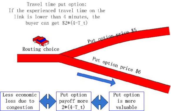
   Figure 1: The price of travel time derivatives indicates short term profit and loss due to traffic conditions: Between two alternative routing choices, a higher derivative price predicts a potentially lower loss and hence the corresponding link is chosen by the traveler.

2. The second type of travel time derivative can be derived based on the cumulative travel time measures for a long time period in the future. For some products of this type, the economic loss due to congestion is less in the coming year if and only if the price is higher. Therefore, the price of travel time derivatives indicates economic loss associated with long-term traffic conditions and a traveler can then plan to use alternative paths or use public transportation if derivative prices are generally low. When considering a long-term transportation plan, travelers can check the price of such derivatives. This category of travel time derivatives is demonstrated in Figure 2 and the CDD index option cited in Table 6 belongs to this category.

   

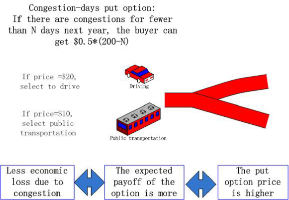
   Figure 2: The price of travel time derivatives indicates profit and loss due to long term traffic conditions: Between two alternative travel plans, a higher derivative price predicts a potentially overall lower loss in a year and hence the traveler chooses to drive.

In this way, travelers’ tolls are based on expected future traffic conditions. If future traffic conditions are expected to be good (bad), the potential future loss is less (more), the payoff is less, and the toll will be less (more). Therefore, travelers could consider taking alternate routes to avoid congestion and reduce travel costs. This flexibility in payment makes the prices of travel time derivatives effective predictors of future travel times. Travelers can forecast the travel time of a path by researching the prices of the corresponding path. This would change traveler behaviors and help them to reduce real-time costs due to traffic delays.

1.5 Travel time derivatives can diversify risk for financial markets

Travel time derivatives can provide new underlings into the investment universe, whose change is relatively independent from existing financial assets. In portfolio theory, the diversification of investments into different asset classes is a recommended practice. For a given set of investments, the lower the correlation between assets, the less the total risk, as in [11]. Most traditional asset classes (equity or bond) are derived from the capital of companies and thus are highly correlated in nature. The correlations between travel time and equity/bond classes are lower than the correlations among different equities/bonds, and the low correlation serves to diversify the portfolio. As investors recognize travel time derivatives as effective risk-reducing elements in their portfolios, they will invest money in the market.

Travel time derivatives have the potential to hedge risks in other markets for derivatives on non-tradable underlyings or commodities. For instance, since weather conditions are correlated with travel time, travel time derivatives could serve as a useful hedging tool for investors who invest in the weather derivative market. Similarly, energy consumption and CO2 emission levels have been traded in the market, and because their performance is highly correlated with that of the traffic system, travel time derivatives could be a useful tool to hedge against risk for investors in these markets.

Moving beyond the transportation sector, during the 2020-2022 period, both traditional financial markets and the crypto market experienced severe stress due to COVID-19 and interest rate hikes implemented to counter high inflation [12] [13]. A new category of derivatives linked to the economy, but not fully subject to the leverage of cryptocurrency or the credit quality of traditional banking, could be a promising hedging tool to help investors navigate future market stress.

2 Potential participants and market making

In light of the necessity analysis outlined earlier, it is important to consider potential participants in travel time derivative markets and the key market-making factors that will need to be addressed. This includes identifying various parties who could benefit from travel time derivatives, such as transportation service providers, government agencies, insurance companies, and institutional investors. Additionally, critical market-making factors that will need to be addressed include designing contracts that are attractive to buyers and sellers, ensuring sufficient liquidity, and developing appropriate pricing models to accurately reflect the risks associated with travel time derivatives. Addressing these factors will be vital to the success of travel time derivative markets.

To provide the hedging effect, there are two types of travel time derivatives for the two sides of the market. Type B: When the specified travel time is expected to be high, a leveraged reward is available to the buyer. Type H: When the specified travel time is expected to be low, a leveraged reward is available to the buyer. Accordingly, participants with different risk profiles will buy different travel time derivatives to hedge their risk; buyers of Type B are the participants who benefit (lose) from good (bad) traffic conditions; buyers of Type H are the participants who lose (who benefit) from good (bad) traffic conditions. The potential participants and their roles are summarized in Table  5.

Table 5: Different participants (B means benefit in good quality of service(QOS); H means hurt in good QOS; market makers and investors can hold both types of derivatives.)

Parameter	Hedging Motivation	Type
Individual travelers	Traffic delay, business delay	B
	extra charges due to bad QOS
Cargo transportation	Traffic delay due to bad QOS	B
	QOS
Tourism industry	Traffic delay due to bad QOS	B
Event organizers	Traffic delay due to bad QOS	B
Municipal management	Traffic delay due to bad QOS	B
Insurance companies	Loss due to vehicle accidents due to bad QOS	B
	Repackaging of vehicle insurance
Gas company	Low overall gas consumption	H
Owners of Toll roads	Low profit due to good	H
	QOS on toll free roads
Vehicle maintenance	Fewer accidents and business loss due to good QOS	H
Auto companies	Fewer needs for new autos due to good QOS	H
Public transportation	Less business due to good QOS	H
Taxi companies	Less business due to good QOS	H
Alternative transportation (train)	Less business due to good QOS	H
Banks	Market Making	B/H
Traffic detection agencies	Measurement providers	B/H
GPS companies
Portfolio managers	Risk diversification	B/H
	Speculation
Project management	Project financing	B/H
	Speculation

As a newly introduced market, the market making of travel time derivatives is critical and challenging, [14]. Market makers match buyers with sellers to enable smooth trading activities; they also provide liquidity to the market by holding short term positions; due to their efforts, the market price of financial derivatives is determined and maintained. To make a profit, market makers quote both a buy and a sell price in derivative contracts, which differ on the bid-offer spread, and they use hedging strategies to control their risk. Investment banks are typical market makers for financial derivatives. With appropriate pricing methods and suitable trading exercise, the total profit for investment banks is positive, which motivates them to operate the business, following the general mechanism in the current financial derivative markets. On the other hand, the counter parties to the market parties will seek protection from the market and their total profit are negative, which can be interpreted as the cost that they pay to hedge risk due to travel time uncertainties in the future. Important factors that should be considered for market making include the following:

1. Market micro structure will be crucial in determining the operation of the market. There are numerous links/paths in transportation networks, and a large number of derivative contracts can be written based on their experienced travel time. Conversely, when this new market begins operating, the trading activity will be low. Therefore, the market may encounter liquidity issues, where smaller trading amounts can drive the prices, and thereby increase price volatility. Several measures can be taken to minimize potential liquidity issues, including restricting the number of products on the market, building temporary liquidity reserves, and so forth. Related discussions for other types of derivatives can be found in [15], [16], [17] and [18] .

2. Market scale is important for the sustainability of the derivatives markets. A survey conducted by the U.S. Department of Commerce in 2004 estimated that approximately 30% of the total U.S. GDP is exposed to some degree of weather risk, [19]. This considerable percentage leads to the necessary liquidity and prosperity of a weather derivative market. In the transportation industry, the percentage needs to be estimated and a larger percentage means more potential market participants. There is significant amount of research on the cost of travel time, which can roughly be measured in the annual revenue raised by road tolls. For example in [20], it is stated "there were $63.2 billion in actual congestion costs in the 85 urban areas [in the U.S.] in 2002. It is estimated that public transportation saved an additional $20 billion in congestion costs for this group." The billion-dollar congestion costs imply a significant impact of traffic delays to individual travelers, which motivates them to hedge their risks. More profoundly, the companies, the profits of which are changed by traffic service, may have more freedom to purchase and trade travel time derivatives, which should be further estimated. The sum of all related profit and costs add to the potential for travel time derivative markets, [21] and [22].

   More recently, According to [23], Transportation plays an important role in the U.S. economy and contributed 8% to U.S. Gross Domestic Product (GDP) in 2020. Transportation is the fourth-largest contributor (behind housing, healthcare, and food) to the national GDP, which measures the monetary value of goods and services in the United States. Per [24], In 2021, the demand for transportation ($1.9 trillion) accounted for 8.4 percent of GDP. Please see Figure 3. While the figures shows GDP directly linked to transportation, there are even more implicit impact of transportation to GDP because the delivery of raw materials and products of a great many other industries rely on quality of service of the transportation system.

   

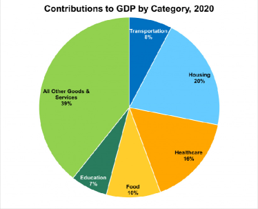
   (a) Contribution to U.S GDP by Category in 2020

   

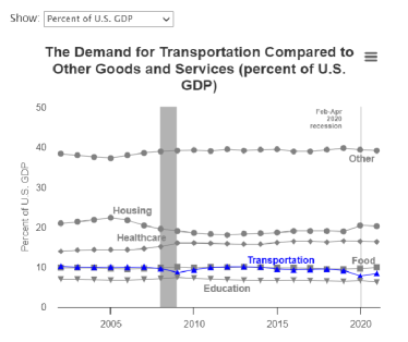
   (b) Contribution of Transportation to U.S GDP over years

   Figure 3: Contribution of Transportation to U.S GDP

3. A healthy market for travel time derivatives also requires appropriate legal regulations. As observed in traditional financial markets, malicious insider trading or market manipulation can occur if the participants know additional information, which may change future travel time through illegal sources. Moreover, unlike traditional underling assets, travel time is the aggregate effect of traveler behavior nearby, so the potential of travel time derivatives in changing traveler behavior may lead to possibility of manipulating future travel times and hence price of travel time derivatives through intentional routing guidance. To prevent such un- desired cases and regulate the travel time derivatives market, appropriate policies or laws should be issued.

Based on the settings above, a market can potentially be established for travel time derivatives. The major products for this potential market are presented in the following section.

3 Design of Travel Time Derivatives

In general, the underlying asset of travel time derivatives is some measure of future travel times. Investors receive cash flows in proportion to travel time related measures as their payoff and in order to purchase such derivatives, investors have to pay a price. Based on the introduction to travel time derivatives in previous sections, several classifications can be applied to travel time derivatives:

1. By contract type, travel time derivatives can be classified into futures, options, etc;

2. By measurement places used in the derivative, they may be classified as derivatives based on one path or several paths, which is hence based on an index of travel time;

3. By the time span of the underlying travel time measures, travel time derivatives can be classified as instantaneous or long term based;

4. By whether the buyer gets a payoff when traffic is good or bad, travel time derivatives can be classified as Beneficial (B) versus Hurting (H).

This section continues to introduce more mathematics for describing the travel time derivatives.

3.1 Standard travel time measurements

In order to define products based on travel time measures, a standard measurement of travel time must be defined.

Theorem 1

A standard measurement of travel time on a specific path and time is the average travel time reported from specific travel time data providers on that path within s small time interval around that time.

Theorem 2

A standard measurement plan of travel time on a specific path on a specific day is a set of standard measurements which are collected at a pre-defined time of day. The daily mean of a standard measurement plan is the mean value of such measurements.

In the above definitions of travel time derivatives market products, all travel time values for a given time in a day are based on a standard measurement, and all travel time values for a given day are based on the standard measurement plan. Each observation is selected by specifying the arrival time to the path. To provide adequate measurements of travel time to support the trading and pricing of travel time derivatives, a loop detector is recommended. The reasons for this choice include:

1. Pricing of travel time derivatives should be based on periodical travel time measurements so that classical stochastic analysis can be used to model travel time and corresponding models can be calibrated. As is summarized in Section 2.1, site-based measurement such as loop detectors can yield such periodical estimations based on occupancy and flow, and hence data from them are suitable for the study of travel time derivatives.

2. Pricing of travel time derivatives should be based on average travel time on the given path to prevent individual measurement error from introducing instability in derivative prices. Loop detectors yield estimation of average travel time based on occupancy and flow, which satisfies this requirement and relieves related concerns.

3.2 Standard spatial travel time index and equivalent return rate

First, a spatial travel time index should be designed. This index can be a weighted average of the latest travel time in downtown areas of major cities in the U.S. A national travel time index is an objective reference for trading and a good symbol for the transportation industry. The definition is given below, and local travel time indexes can be designed in a similar fashion.

Theorem 3

Spatial Travel Time Index

$$T_{us}=\sum T_{i}*\alpha_{i}$$

where $T_{i}$ is the travel time in selected places within a given area.

For example, a Spatial Travel Time Index could be constructed as the weighted average of the realtime travel time in downtown New York (a section of Fifth Avenue), downtown Chicago (a section of Michigan Avenue), downtown Los Angeles (a section of Sunset Boulevard), and downtown Houston (a section of Main Street). This index can be viewed as an average traffic index on the quality of service of the urban transportation system in the United States, which shows the national service level of urban traffic systems. The return of this index, volatility, and its sharpe ratio can then be used as references when pricing travel time derivatives. Note the Sharp ratio is the ratio between access return and volatility of this derivative, and excess return is the extra return of this index relative to the risk-free bond.

Travel time indexes can also be defined for a given area, if taking the average travel time in the major avenues of Manhattan can be used to indicate the general traffic conditions on Manhattan island. Travelers can trade over such indexes to compensate for the waste of time and economic loss due to traffic delays.

To provide a more practical example, a U.S. Congestion Day index futures contract can be defined in a similar fashion as the Canadian Degree Days index HDD futures contract displayed in Table 6. In this contract, the average daily travel time (which can be measured using certain sampling schemes) minus a predefined travel time value floored at zero is summed over a given calendar month for several urban transportation routes in the U.S. Suppose the buyer purchases the contract at price P; initially, if travel times on the specified urban routes are generally higher and this sum is potentially higher in a given month, the price of the contract would increase. In this case, the buyer profits from the price increase and increased payoff G-P to compensate potential losses due to high travel time. This contract can be designed and traded in a similar fashion as that for weather derivatives. Note that related mechanisms are discussed in more detail in the subsequent sections, beginning with more basic products.

Table 6: US Congestion Days Index (CDD) Futures

Contract Size	US $20 times the respective
	CME USA Congestion Days Index
Index Product Description	Congestion Degree Days (CDD)
	for U.S. Cities
Measurement definition	The travel time in a particular city is reported
	based on a specific route:
	along Fifth Avenue between 59th st
	and Washington Square, New York
	along Michigan Avenue between South Lake Drive
	and Roosevelt Road,Chicago
	along Sunset Boulevard between Prospect Ave
	and Harbar Highway, Los Angeles
	along Main Street between Bissonnet St
	and Commence St, Houston
Pricing Unit	US Dollars (US $) per index point
Tick Size	1 index point
(minimum fluctuation)	(= US $ 20 per contract)
Trading Hours	CME Globex (Electronic Platform)
(All times listed are Central Time)	SUN 5:00 p.m. - FRI 3:15 p.m.
	Daily trading halts 3:15 p.m. - 5:00 p.m.
Last Trade Date/Time	Fifth Exchange business day
	after the futures contract month, 9:00 a.m.
Position Limits	All months combined: 10,000 contracts
	See CME Rule 42102.D.
Exchange Rule	These contracts are listed with,
	and subject to, the rules and regulations of CME.

3.3 Design of derivative products on travel time

Type 1 Basic options for a specific link at a given future time point

The simple derivative based on the experienced travel time at a future time is defined as follows, and an example is given afterwards.

Theorem 4

Call option on a certain travel time. Consider the link $l$ a specific time instant $t$ in the future. If the travel time shown by the standard measurement at $t$(denoted as $T$) is higher than a given $K$, then there is a payment $\alpha(T-K)$ to the option buyer; if lower, there is no payment.$\alpha$ is the leverage coefficient.

Theorem 5

Put option on a certain travel time. Consider the link $l$ a specific time instant $t$ in the future. If the travel time shown by the standard measurement at $t$(denoted as $T$) is lower than a given $K$, then a payment $\alpha(K-T)$ is available to the option buyer ; if higher, there is no payment.$\alpha$ is the leverage coefficient.

Consider Broadway in New York City from 20th to 60th Streets. If the travel time shown by its standard measurement entering at 10 a.m. on January 1, 2011, is equal to 70 minutes and the threshold value is set as 60, then there is a leveraged cash back to the buyer $ $10**(70-60)$; if the experienced travel time is lower than 60 minutes, the buyer gets nothing.

Type 2 Futures on congestion-days

After establishing basic options for a specific link at a given future time point, the futures written on the high congestion days (HCD) and low congestion days (LCD) are then designed. As a basic concept, the definitions of HCD and LCD are given below:

Theorem 6

High Congestion Days(HCD) and Low Congestion Days(LCD) in discrete time settings

Let $T_{i}$ denotes the mean of a standard measurement plan on day $d_{i}$ and $C$ as a specified reference value. The high congestion-days, $HCD_{i}$, and the lower congestion-days, $LCD_{i}$, on that day are defined as $HCD_{i}=max(T_{i}-C,0)$ and $LCD_{i}=max(C-T_{i},0)$ respectively. In other words, $HCD$ is the extra amount of travel time spent on that day compared to the reference value $C$, and $LCD_{i}$ is the amount of travel time savings compared to the reference value $C$.

Then the HCD for a given time period $[t_{1},t_{2}]$ is defined as the sum of the HCD on all the days in that period, given a fixed number of measurements.

$$HCD(t_{1},t_{2})=\sum_{i=1}^{n}HCD_{i}1_{d_{i}\in[t_{1},t_{2}]}$$

The LCD for a given time period $[t_{1},t_{2}]$ is defined as the sum of the LCD on all the days in that period, given a fixed number of measurements.

$$LCD(t_{1},t_{2})=\sum_{i=1}^{n}LCD_{i}1_{d_{i}\in[t_{1},t_{2}]}$$

, as the HCD/LCD for the time period.

In a continuous setting, the payoff functions should be defined as follows:

Theorem 7

High Congestion Days(HCD) and Low Congestion Days(LCD) in continuous time

Given a threshold $T$, the HCD for a given time period $[t_{1},t_{2}]$ is defined as

$$HCD(t_{1},t_{2})=\int_{t1}^{t2}max(T_{t}-T,0)dt$$

the LCD for a given time period $[t_{1},t_{2}]$ is defined as

$$LCD(t_{1},t_{2})=\int_{t1}^{t2}max(T-T_{t},0)dt$$

This pair of products shows the cumulative performance of the path compared to some average reference. Its price will reflect market participants’ expectations of the quality of service on the path; hence, its price can predict the long term traffic status on the path.

Type 3 Congestion-days options

Congestion days options are options based on the average performance of a path in a future time window. The definitions are given first, followed by an example.

Theorem 8

Call options on high congestion days. Denote $K$ as the strike value:

The payoff of a HCD call is

$$V=\alpha max(H_{n}-K,0)$$

The payoff of a LCD Call is

$$V=\alpha max(L_{n}-K,0)$$

Theorem 9

Put options on high congestion days. Denote $K$ as the strike value:

The payoff of a HCD put is

$$X=\alpha max(K-H_{n},0)$$

The payoff of a LCD put is

$$X=\alpha max(K-L_{n},0)$$

Consider Broadway in New York City from 20th to 60th Streets. If the mean travel time on it is greater than 60 minutes, then a surplus $T-60$ is recorded as a congestion day; otherwise 0 surplus is recorded. Then all these surplus values are added together for one year with 365 days. If the sum $S$ equals 2000 and so is larger than $K=1500$, then there is a leveraged cash back $10*(S-K)$ where 10 is the leverage ratio; if not, the buyer receives nothing. This is an example of an HCD call option. This pair of products leverages the buyer’s gain according to long term traffic status in the future. Compared to the futures, the options provide further leverage, and the buyers can get more return/loss if traffic conditions change. In buying such products, a traveler will change travel patterns accordingly. In this sense, options on travel time are effective in changing a traveler’s behavior.

Type 4 Futures on cumulative travel time

This product is the futures contract written on the cumulative travel time in a future time period. The cumulative travel time index is defined first.

Theorem 10

Cumulative travel time index (CTT) in discrete time settings.

The CTT index over a time interval $[t_{1},t_{2}]$ is defined as the sum of the daily standard measurement plan in a given time period.

$$CTT(t_{1},t_{2})=\sum_{i=1}^{n}T_{t_{i}}I_{t_{i}\in[t_{1},t_{2}]}$$

.

Theorem 11

Cumulative travel time index in a future time period(CTT) in continuous time settings.

The CTT index over a time window $[t_{1},t_{2}]$ is defined as the integration of travel time in that time window.

$$CTT(t_{1},t_{2})=\int_{t1}^{t2}T_{t}dt$$

The payoff of the futures on CTT is in direct proportion to the travel time that a traveler experiences over a given time period. It is an alternative measure of the long term quality of service to HCD/LCDs.

Type 5 Options on cumulative travel time These products are the options written on the CTT index. Their payoff functions are given as follows:

Theorem 12

Call options on cumulative travel time. Denote $K$ as the strike value: The payoff of a HCD call is

$$V=\alpha max(CTT-K,0)$$

Theorem 13

Put options on high congestion days. Denote $K$ as the strike value: The payoff of a HCD put is

$$X=\alpha max(K-CTT,0)$$

Again, the options on CTT provide greater leverage than other forms of road tolls; therefore, they can potentially change a traveler’s behavior more effectively.

4 Pricing derivatives on travel time

To price travel time derivatives, the underlying travel time series is first selected as a continuous time mean reverting process with trend and seasonality adjustments. Due to variation in traffic conditions across different links, the travel times on different links may be fitted to models with different orders. To provide such flexibility, a family of alternative models are introduced in this section. Model selection is conducted based on empirical data according to statistical principles and pricing methods are discussed.

4.1 Alternative stochastic processes for modeling travel time

This section provides an overview of relevant stochastic processes used for modeling time series data similar to road travel time and pricing financial derivatives based on non-tradable underlyings. Mean reverting processes are frequently used in financial literature to model time series that tend to move back to their average over time, such as interest rates and weather derivatives [25]. For example, Benth and Benth (2007) [26] analyzed weather derivatives traded at the Chicago Mercantile Exchange and modeled temperature dynamics as a continuous-time autoregressive process, allowing for pricing of futures and options on weather. In Gyamerah (2019) [27], a machine learning model was used to identify drivers of maize yield, and a mean-reverting model was proposed with a time-varying speed of mean reversion, seasonal mean, and local volatility that depended on local average temperature. Alfons (2022) [28] developed a stochastic volatility model for average daily temperature, which was calibrated using daily data from eight major European cities, and pricing was done using Monte-Carlo and Fourier transform techniques.

Alternatively, local risk minimization indifference pricing is also a promising methodology for pricing derivatives under incomplete markets. Rene (2013) [29] used the local risk minimization approach to price and hedge energy derivatives in incomplete markets by specifying the set of infinitely many equivalent martingale measures and identifying the minimum measure with zero risk premium. Chen (2021) [30] studied utility indifference pricing of derivatives based on untradable assets in incomplete markets using a symmetric asymptotic hyperbolic absolute risk aversion (SAHARA) utility function.

To model travel time, similar stochastic processes can be used, and specific patterns of travel time are considered in the fitting process. Ke (2009)[31] introduced the idea of financial derivatives based on travel time, and further work on the properties and pricing methodology was summarized in Ke (2014)[32]. Theoretical foundations for discrete ARMA models are summarized in detail in Janqing(2017) [33], and background on continuous ARMA processes is provided by Brockwell (2001) [34] and Brockwell (2010) [35].

4.1.1 Continuous autoregressive moving average (CARMA) process

Let $(\Omega,\mathcal{F},{\mathcal{F}}_{\{t>0\}},P)$ be a complete filtration probability space. A random variable is a mapping $X:\Omega\rightarrow R^{d}$, if it is $F$-measurable, whereas a family of random variables depending on time t, ${X_{t}}_{t>0}$ is said to be a stochastic process. A process $X_{t}$ is $F$-adapted if every $X_{t}$ is measurable with respect to the $\sigma$-algebra $F$.

Then a continuous-time Gaussian autoregressive and moving average process (CARMA) can be used to fit the travel time process The process $X_{t}$ in previous section is the simplest CARMA($1,0$) process. By definition, a CARMA process $Y_{t}$ is defined symbolically to be a stationary solution of the stochastic differential equation:

$$a(D)C_{t}=b(D)B_{t}$$

with coefficients $a_{1},a_{2},\cdots,a_{p}$ and $b_{0},b_{1},\cdots,b_{q}$ for $p>q$

$a(z)=a_{0}z^{p}+a_{1}z^{p-1}+\cdots+a_{p}$

$b(z)=b_{0}+b_{1}z+\cdots+b_{q}z^{q}$

The operator $D$ denotes differentiation with respect to $t$, which is in the formal sense for the Brownian Motion [34]. Due to the fact the derivative of $B_{t}$ does not exist with probability 1, the process is represented further in the following state space representation

$$C_{t}=BX_{t}$$

and

$$dX_{t}=AX_{t}dt+edB_{t}$$

with

$B=[b_{0},b_{1},\ldots,b_{q},0,\ldots,0]$

$X_{t}=(X_{t,0};\ldots;X_{t,p-1})$ and the first $p-1$ element of $X_{t}$ is defined as

$$X_{t,j}-X_{0,j}=\int_{0}^{t}X_{u,j+1}du$$

$A$=

$$\left[\begin{array}[]{ccccc}0&1&0&\cdots&0\\ 0&0&1&\cdots&0\\ \vdots&\vdots&\vdots&\ddots&\vdots\\ 0&0&0&\cdots&1\\ -a_{p}&-a_{p-1}&-a_{p-2}&\cdots&a_{1}\end{array}\right]$$

$\textbf{e}=[0,0,0,0,0,0,1]^{T}$

when $p=1$, $A$ is defined as $-a_{1}$

By applying the multidimensional Ito Formula, the solution to the S.D.E above is below:

$$X_{t}=e^{At}X_{0}+\int_{0}^{t}e^{A(t-u)}\textbf{e}dB_{u}$$

The process above is stationary and well defined when $p>q$. If $p\leq q$, the covariance function does not exist and the spectral density does not exist. However, the process is further defined as a general random process (GRP) by Brockwell (2010) [35] for the study of the derivatives of CARMA($p,q$) processes. In the following sections, the paper focuses on the continuous time derivative pricing based on CARMA($p,q$) process for the $p>q$ case, while it is recommended that Monte Carlo simulation be conducted based on the fitted discrete time models to approximate the derivative prices for if $p\leq q$.

4.2 Modeling travel time processes

In this subsection, empirical data are used to select the model to describe travel time processes, and corresponding parameters are estimated. The driving process is identified as an ARIMA model, and corresponding continuous versions are given. The model is then used to price derivatives in later sections. First, the mean reverting model is re-parameterized as follows:

$$T_{t}=r_{t}+s_{t}+Y_{t}\mbox{, }t=0,1,2,\ldots$$ (1)

where $r_{t}$ is the trend part, $s_{t}$ is the season part, and $Y_{t}$ is the driving process that shapes the noise term. Define $c_{t}=r_{t}+s_{t}$ as the sum of the trend and seasonal parts. The terms are explained separately as follows:

1. The trend part is a linear function over time

   $$r_{t}=a+bt$$

2. Seasonal parts are as follows:

   $$s_{t}=b_{t}+w_{t}$$

   1. The daily part is:

      $$b_{t}=k+\sum_{1}^{I_{s}}a_{t}(sin2i\pi(t-f_{i})/T_{d}+\sum_{1}^{J_{s}}b_{t}(cos2i\pi(t-g_{i})/T_{d})$$

   2. The weekly part is:

      $$w_{t}=k+\sum_{1}^{I_{s}}a_{t}(sin2i\pi(t-f_{i})/T_{w}+\sum_{1}^{J_{s}}b_{t}(cos2i\pi(t-g_{i})/T_{w})$$

   3. Another alternative is the 10-parameter model given in [36]:

      $$V(t)=\mu+\sum_{i=1}{3}k_{i}\phi(t,\mu_{i},\sigma_{i})$$

      However, the trigonometric functions are selected as the basis function, because they are orthogonal and suitable to describe the periodical pattern of travel time.

3. $Y_{t}$ is the driving process. It is a stochastic process and the type of process is determined based on empirical data. For the data in this section, it is defined that $C_{t}=dY_{t}$ and $C_{t}$ is modeled as a CARMA($p,q$) process.

The data set is the travel time data set from California PEMS. Data were collected in November 2012, on the 80-E path between 80-E/Cummings Skwy and 80-E/Maritime Academy, as presented in Figure 4. The travel time data are gathered from loops captured every 5 minutes. The calibration process is as follows:

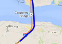
(a) The path

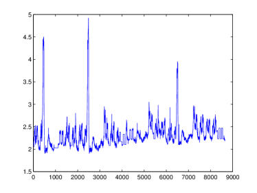
(b) The original data

Figure 4: Experiment Network and Sample Travel Time Data

1. A regression estimate is generated for the trend over the year in the table, and the estimate is not significant except as a stable mean function $a=2.23$. This part is shown in the Figure 5.

2. The seasonal model is studied using a regression method. The parameters for the two seasonal models are obtained as follows with T as 2064 for the weekly pattern and 288 for the daily pattern. The fitted parameters are displayed in Table 7 and the seasonal parts are shown in Figure 5.

   Table 7: Seasonal effects in the 80E data

   Weekly trend	$k$	$a_{1}$	$a_{2}$	$a_{3}$	$b_{1}$	$b_{2}$	$b_{3}$	T
   	0.0927	-0.0135	0.0794	-0.0902	0.0477	-0.0873	-0.0228	2064
   Daily trend
   	0.0002	0.0240	0.1143	-0.0795	-0.1509	0.0127	-0.0204	288

   

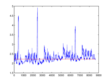
   (a) Mean function over time

   

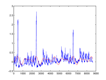
   (b) The weekly pattern

   

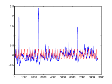
   (c) The daily pattern

   

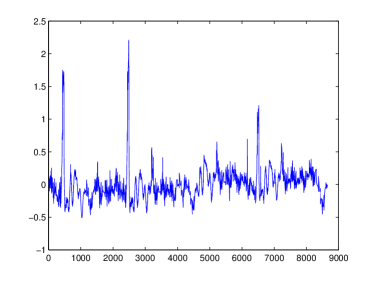
   (d) The residual

   Figure 5: Remove the trend, weekly, daily part of 80E data series

3. After removing the trend and seasonal part, the residual is used to estimate the CARMA($p,q$) process. In the literature, the methods to estimate CARMA($p,q$) models can be based either directly on the continuous-time process or on a discretised version. The latter relates the continuous-time dynamics to a discrete time ARMA process. The advantage of this method is that standard packages for the estimation of ARMA processes may be used in order to estimate the parameters of the corresponding CARMA process. However, not every ARMA($p,q$) process is embeddable in a CARMA($p,q$) process. Brockwell and collaborators devote several papers to the embedding of ARMA processes in a CARMA process, [37] and [38]. In the study below, this approach is employed by assuming an appropriate class of CARMA processes to work with.

   Following the intuition above, the residual is identified as the following ARIMA(1,1,0) model (Table 8). A Box-Ljung test suggests that the p-value $=0.1928$. This model describes the time series well.

   

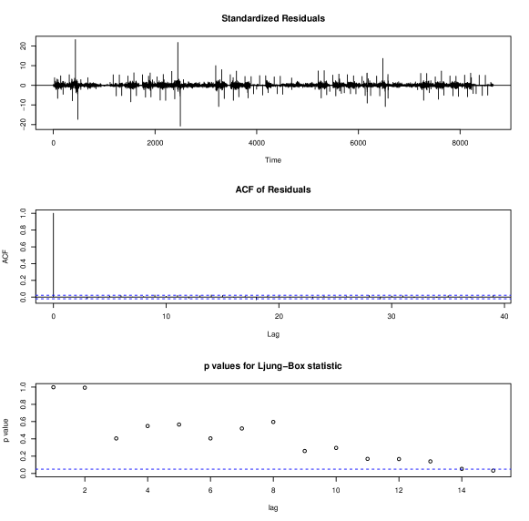
   Figure 6: 80E ARIMA model

   Table 8: Model selection for 80E data

   	Log Liklihood	AIC	p-value of Box-Ljung test
   ARIMA($1,0,0$)	14467.36	-28928.72	0.0035
   ARIMA($1,1,0$)	14438.3	-28872.61	0.1928
   ARIMA($1,1,1$)	14438.31	-28870.61	0.1322
   ARIMA($2,1,1$)	14438.31	-28868.61	0.0840

   The model is described as the ARIMA($1,1,0$) model by comparing the test results, and additional variance modeling can be conducted to describe the volatility process.

4. The estimation is demonstrated for a selected path above, in which the model follows ARIMA($1,1,0$). However, travel time processes for different paths may appear to fit ARIMA models with different orders (Table 9). To address such variations, the pricing of travel time derivatives is discussed considering all possible orders of ARIMA models. Particularly, distinct treatments are applied conditioned on whether $p>q$ holds or not. In more detail, the spectral density for a CARMA($p,q$) process is defined as

   $$f(\omega)=\frac{\sigma^{2}\beta(i\omega)\beta(-i\omega)}{2\pi\alpha(i\omega)\alpha(-i\omega)}$$

   The stationarity condition of the CARMA processes requires the roots of the polynomial $\alpha(z)$ to have negative real-parts and that $p>q$, [39]. Below the estimation of CARMA($p,q$) processes are conducted based on fitted ARMA model considering different relations of $p$ and $q$:

   Table 9: Models with best fit for different paths

   Path Name	Model	p-value of Box-Ljung test
   Cummings Skwy - Maritime Academy	ARIMA($1,1,0$)	0.1928
   Berkeley-Davis	ARIMA($2,1,1$)	0.0503
   Lincoln-Davis	ARIMA($1,1,1$)	0.3419

   1. If $p>q$, the discrete solution for the CARMA($p,q$) state space representation can be given as the following equation

      $$x_{t+\delta t}=e^{A\delta t}x_{t}+\int_{t}^{t+\delta t}e^{t+\delta t-u}e_{p}\sigma_{u}dB_{u}$$

      The noise term is of variance $\int_{0}^{\delta t}e^{Au}e_{p}e_{p}^{t}e^{A^{t}u}du$. If first order expansion of the matrix exponential $e^{Au}$ is taken, a set of formulas can be derived to map the parameters of the CARMA($p,q$) processes ($\alpha_{n}$,$\beta_{n}$) approximately to the parameters of the corresponding discrete ARMA($p,q$) models ($a_{n}$,$b_{n}$), [40]. Correspondingly, the parameters of the CARMA($p,q$) processes can be backed out using estimated ARMA model parameters: Assuming the grid size is $h$, the mapping for the auto regression parts of the model in the first three orders is displayed in Table 10.

      
      
      
      

      Table 10: Coefficients mapping between discrete and continuous ARMA models

      Model	Formula
      CAR(1)	$a_{1}=1-\alpha_{1}h$
      CAR(2)	$a_{1}=2-\alpha_{1}h$
      	$a_{2}=\alpha_{1}h-\alpha_{2}h-1$

      The estimation of the moving average parameters can be based on auto correlation function [41] and a least absolute deviation algorithm can be used to estimate the MA part based on the empirical and theoretical autocorrelation functions of the CARMA processes.

      $$\gamma(s)=b^{t}e^{A|s|}\Sigma b$$

      where

      $$\Sigma=\int_{0}^{\infty}e^{Au}e_{p}e_{p}^{t}e^{A^{t}u}du=-A^{-1}e_{p}e_{p}^{t}$$

      In this representation, $A^{-1}$ is the inverse of the operator A : $X\rightarrow AX+XA^{t}$, [42] and [43].

      With these mapping formulas, the coefficients of the continuous ARMA processes can be solved using the parameters of the fitted discrete ARMA model. These mappings ignore higher order terms and can hence be applied to low order CARMA processes for engineering purposes. These values can also be used as the initial values for more precise estimation of the CARMA parameters.

      To obtain such precise estimations, a Kalman filter is used to further extract the unobserved states of the CARMA ($p,q$) processes based on the state-space representation and parameters are estimated by minimizing the error between observed and estimated output series of the state space model. In more detail, given a travel time series whose trend and seasonality are removed, first order differentiation is taken to remove the integrated part of the model. The remaining process $X_{t}$ is then processed using a Kalman filter to extract the unobserved higher order states in the CARMA process, [44] and [45]. The filtered model produces an output series $X^{\prime}_{t}$ and the mean square error of $X_{t}$ and $X^{\prime}_{t}$ are minimized to yield the minimum mean-squared-error linear predictors for the parameters of CARMA($p,q$), which is found by numerically minimizing the sum of squares. To obtain a warm start, the parameters obtained from the previous first order approximation are used as initial values. The estimated parameters are displayed in Table 11 and the estimated processes need to be calibrated further to the market to determine the market value of risk $\theta$, using the methods discussed in next section.

      Table 11: Coefficient estimation for discrete and continuous time ARMA models

      Path	Parameter	ARMA	Initial Value	Estimated Value
      Cummings Skwy -	AR-1	-0.0326	0.2065	0.2512
      Maritime Academy
      Berkeley-Davis	AR-1	0.9646	0.2071	0.1780
      	AR-2	-0.1275	0.03258	0.0685
      	MA-1	-0.6575	0.1356	-0.6296

   2. For the processes corresponding to the case of $p\leq q$, for example, the ARIMA($1,1,1$) on path Lincoln-Davis, it is recommended that Monte Carlo method based on the discrete ARIMA model be used to price the travel time derivative after the pricing principles and risk neutral measure are specified. Although CARMA ($p,q$) has recently been extended into generalized random processes for cases when $p\leq q$, [35], the processes under such settings are not well defined in the usual sense. In terms of rationale, the general random process yields a way to represent the discrete approximation of the high order derivatives of Ornstein - Uhlenbeck process with respect to selected linear functionals, but this representation does not lead to typical continuous time stochastic models. The application of a generalized random process for pricing travel time derivatives is still contingent upon further studies of such processes and hence the Monte Carlo method is a reasonable approximation for modeling and pricing travel time derivative.

In summary, travel time processes are fitted to discrete ARMA($p,q$) models with trend and seasonality adjustment first. Then the fitted models are converted into stable CARMA($p,q$) processes for further calculation when $p>q$. When $p\leq q$, it is recommended that Monte Carlo simulation based on the discrete ARMA models be used to price travel time derivatives. In the following sections, potential pricing schemes are discussed based on fitted CARMA($p,q$) processes.

4.3 Risk neutral pricing in an incomplete market

To obtain a general pricing expression for travel time derivatives, risk neutral pricing principle in incomplete market conditions is employed in this section, deploying the method in [46].

4.3.1 Risk neutral representations

A risk-neutral probability is by definition a probability measure $Q\sim P$ such that all tradable assets in the market are martingales after discounting. Thus, all equivalent probabilities $Q$ will become risk-neutral probabilities. A sub-family of probability measures $Q$ is specified using the Girsanov transformation: assume $\omega_{t}$ is a real-valued measurable and $\frac{\omega_{s}}{\sigma_{s}}$ is a bounded function. The stochastic process:

$$Z^{\omega}(t)=exp(\int\frac{\omega_{s}}{\sigma_{s}}dW_{s}-\frac{1}{2}\int\frac{\omega^{2}_{s}}{\sigma^{2}_{s}}ds)$$

is the density process of the probability measure $Q$. Under $Q$, the process

$$dB_{t}=dW_{t}-\frac{\omega(s)}{\sigma(s)}dt=dW_{t}-\theta_{t}$$

is a Brownian motion and $\theta_{t}$ is called the market value of risk process. Based on this measure change, the dynamics of the underlying process under the risk neutral measure are given by the following S.D.E:

$$dT_{t}=dc_{t}+\omega(t)dt+a_{t}(c_{t}-T_{t})dt+\sigma_{t}dW_{t}$$

and the solution to this S.D.E is then

$$T_{t}=c_{t}+(T_{0}-c_{0})e^{-\int_{0}^{t}a_{s}ds}+e^{-\int_{0}^{t}a_{s}ds}\int_{0}^{t}e^{\int_{0}^{u}a_{s}ds}\omega_{u}du+e^{-\int_{0}^{t}a_{s}ds}\int_{0}^{t}e^{\int_{0}^{u}a_{s}ds}\sigma_{u}dW_{u}$$

When the coefficients are constant, the general solution reduces to the following simpler form:

$$T_{t}=c+(T_{0}-c)e^{-at}+\int_{0}^{t}e^{-a(t-u)}\omega_{u}du+\int_{0}^{t}e^{-a(t-u)}\sigma dW_{u}$$

Then the prices of different travel time derivative contracts in continuous time are calculated as the discounted expectation of their corresponding payoff function under this measure, which is given below:

The price of a HCD futures contract can be calculated as:

$$F_{HCD}(t_{1},t_{2},T,t)=E_{Q}\left\{\int_{t1}^{t2}max(T_{s}-T,0)ds|\mathcal{F}_{t}\right\}$$

The price of a LCD futures contract can be calculated as:

$$F_{LCD}(t_{1},t_{2},T,t)=E_{Q}\left\{\int_{t1}^{t2}max(T-T_{s},0)ds|\mathcal{F}_{t}\right\}$$

Assuming a constant interest rate, the price of a HCD call options contract can be calculated as:

$$C_{HCD}(t_{1},t_{2},T,t,K)=e^{-rt}E_{Q}\left\{max(\int_{t1}^{t2}max(T_{s}-T,0)ds-K,0)|\mathcal{F}_{t}\right\}$$

and the price of a LCD call options contract can be calculated as

$$C_{LCD}(t_{1},t_{2},T,t,K)=e^{-rt}E_{Q}\left\{max(\int_{t1}^{t2}max(T-T_{s},0)ds-K,0)|\mathcal{F}_{t}\right\}$$

The price of a CTT futures contract can be calculated as:

$$F_{CTT}(t_{1},t_{2},t)=E_{Q}\left\{\int_{t1}^{t2}T_{s}ds|\mathcal{F}_{t}\right\}$$

Assuming a constant interest rate, the price of a CTT call options contract can be calculated as

$$C_{CTT}(t_{1},t_{2},t,K)=e^{-rt}E_{Q}\left\{max(\int_{t1}^{t2}T_{s}ds-K,0)|\mathcal{F}_{t}\right\}$$

Since travel time is neither a tradable nor storable asset, the derivatives contracts cannot be hedged using travel time itself in the financial markets, and the market of the travel time derivatives is therefore incomplete. Under such incomplete markets, the risk neutral measure is not unique. To obtain the prices, the risk neutral measure should first be specified considering the characteristics of the incomplete market setting. Moreover, the expectation can be calculated using two alternative methods: it can be calculated using Monte Carlo simulation of the underlying processes under the specific risk neutral measure, the average discounted payoff of the financial derivative in all paths yield the price of the contract; alternatively, some explicit formulas can be obtained by considering the property of the discounted price processes under the risk neutral measure.

4.3.2 Determination of the risk neutral measure

The incompleteness of the travel time derivative market requires the estimation of the market price of risk (MPR) for pricing and hedging travel time derivatives. The market price of risk adjusts the underlying process representing travel time so that the implied price is arbitrage free. As it is stated in Section 5.4.3, $B_{t}=W_{t}-\theta_{t}$ is a Brownian motion under the risk neutral measure. Since the underlying asset is not tradable, there is no unique risk neutral measure. The drift of the asset price process is the view of the trader about the growth of the process. There are different ways of specifying this measure and some of them are discussed below:

1. Market value of risk can be inferred from market traded products. [40] suggests inferring the market price of risk(MPR) from traded CAT futures by minimizing the mean square error between the modeled contract prices with the market traded prices. Once the MPR for temperature futures is known, it is used to price other derivatives. According to [47], within incomplete markets, there may exists many equivalent risk-neutral measures; it is the job of the market as a whole, via trading of derivatives, to decide which measure prevails at any one given point in time. A class of equivalent martingale measures can be identified which maintains the structure of real-world dynamics for asset prices. These measures can then be used to obtain forward prices and value spread option. Moreover, the differences in pricing measures leads to risk premium which can be calibrated using market prices: [48] showed a negative market price of risk associated to the non-stationary term in their two-factor models, when analyzing data from energy market. In the proposed two-factor model, where the non-stationary term is a drifted Brownian motion, the negative market price of risk appears as a negative risk-neutral drift. [49], showed that using the certainty equivalence principle that the presence of jumps in the spot price dynamics will lead to a positive risk premium in the short end of the futures curve. [50] explain the existence of a positive premium in the short end of the futures market by an equilibrium model.

   In the context of travel time derivatives, the choice of $\theta_{t}$ uniquely determines the equivalent martingale measure under which derivatives pricing is performed. One way of defining the market price of risk is to extrapolate from option prices. This technique resembles recovery of the implied volatility in the Black-Scholes model. A chosen objective function can be minimized to find $\theta_{t}$, such as the mean absolute percentage error between the market and model option prices. The market prices can be chosen as averages of the bid and ask offers and options with different strikes can be used to calibrate $\theta_{t}$ for a given day. Alternatively, calibrating it to futures prices is also feasible. The procedure is analogous to that used with options, and the model can be calibrated to one futures price. Futures have more liquidity than options and hence allow for a more frequent and precise calibration of $\theta_{t}$. The value of $\theta_{t}$ is subject to the incentive for hedging on the demand side relative to the supply side. For a concrete example, the market value of risk process $\theta_{t}$ can be calibrated by a set of HCD futures contracts based on the common underlying travel time series by minimizing the mean squared difference between modeled price and traded price below

   $$\theta_{t}=argmin(\sum_{i}(F_{i,market}-F_{i,HCD}(t_{1},t_{2},T,t,\theta_{t}))^{2})$$

   Different contracts can be used to conduct such calibration and contracts with the most liquidity in the market are the best instrument for such purposes.

2. Suitable hedging strategies result in a price, that suggests a risk neutral measure. Different hedging strategies leads to varying derivative prices.

3. Some characteristics of the risk neutral measure can be specified based on certain optimality conditions. For example, the minimum entropy measure has been studied in [51], as it can yield reasonable asset prices and there is a huge literature on the use of maximum entropy measure for calibration purposes. In [52], a minimal martingale measure based on local variance minimization provides a strategy that penalizes over-hedging. [53] introduces pricing methods based on suitable risk measures and partial hedging is used when certain risk measures are introduced to control the residual risk at expiration. Such methods can be applied to identify the best pricing measure for pricing travel time derivatives.

These methods may lead to different prices due to the non-tradable nature of travel time. This discussion again shows that the prices of travel time derivatives are subject to the choices of specific hedging strategies, under incomplete market conditions with non-unique risk neutral measures. In the following section, it is assumed that a risk neutral measure can be calibrated using the price of traded derivatives.

4.3.3 Risk neutral pricing for travel time derivatives

In this section, pricing P.D.Es are further derived based on the pricing measure that is identified using methods in the previous section. The rationale is that derivative prices are functions of underlying processes and these prices should be martingales under the specified risk neutral measure. To provide some background, a martingale is a stochastic process for which, at a particular time in the realized sequence, the expectation of the next value in the sequence is equal to the present observed value even given knowledge of all prior observed values at the current time. Based on this rationale, Proposition 8.1 of [54] introduces the martingale P.D.E condition for a stochastic process, which suggests the drift term should be zero for a martingale process. As the mathematic derivatives of the price function can be calculated, the martingale condition above leads to partial differential equations (P.D.E) which yields the analytical solution for the prices of travel time derivatives. In the following analysis, the prices based on simple CARMA($1,0$) processes with first order integration are first discussed and then extended to general CARMA($p,q$) processes with first order integration and with $p>q$; $Y_{t}$ is obtained by removing trends and seasonal adjustments from the original travel time series.

Theorem 14

For the Asian type call option on the process $Y_{t}$, where $Y_{t}=\int_{0}^{t}X_{u}du$ and $X_{t}$ is a CARMA($1,0$) process, its price can be solved via the following P.D.E by further expanding states as follows:

$$v_{t}(t,x,y,z)+A(t,X_{t})v_{x}(t,x,y,z)+xv_{y}(t,x,y,z)+yv_{z}(t,x,y,z)+\frac{1}{2}B(t,X_{t})^{2}v_{xx}=rv(t,x,y,z)$$

$0\leq t<T$,$x\in R$,$y\in R$,$z\in R$

with boundary conditions:

$$lim_{z\rightarrow-\infty}v(t,x,y,z)=0,0\leq t<T,x\in R,y\in R$$

$$v(T,x,y,z)=(z-K)^{+},x\in R,y\in R,z\in R$$

$$v(t,0,0,z)=e^{-r(T-t)}(z-K)^{+},t<T,z\in R$$

Proof:

Consider the claim $(Z_{t}-K)^{+}$, under the risk neutral measure $Q$, we have:

$$dZ_{t} = Y_{t}dt$$

$$dY_{t} = X_{t}dt$$

$$dX_{t} = A^{*}(t,X_{t})dt+B(t,X_{t})dW_{t}$$

We consider that this group of differential equation defines a three dimensional Markovian process. The value of the derivative contract will be $P=de^{-rt}v(t,x,y,z)$. By Ito’lemma, it is subject to the following dynamics:

$$dv(t,x,y,z) = v_{t}dt+v_{x}dx+\frac{1}{2}v_{xx}d<x>+v_{y}dy+v_{z}dz$$

$$dP = e^{-rt}(-rv+v_{t}+\frac{1}{2}v_{xx}B(t,X_{t})^{2}+v_{x}A^{*}(t,X_{t})+xv_{y}+yv_{z})dt+v_{x}B(t,X_{t})e^{-rt}dW_{t}$$

The discounted price process should be a martingale under the risk neutral measure, so we have

$$-rv+v_{t}+\frac{1}{2}v_{xx}B(t,X_{t})^{2}+v_{x}A^{*}(t,X_{t})+xv_{y}+yv_{z}=0$$

That is

$$v_{t}+\frac{1}{2}v_{xx}B(t,X_{t})^{2}+v_{x}A^{*}(t,X_{t})+xv_{y}+yv_{z}=rv$$

Here $A^{*}(t,X_{t})$ is the drift of $X$ under the risk neutral measure.

For the boundary conditions, as $Y_{t}$ is obtained by removing trends and seasonal adjustments from the original travel time series, it can be negative. All the state variables corresponding to the CARMA($1,0$) process can be in $R$.

If $Y(t)$ approaches $-\infty$, then the probability that the call expires in the money approaches zero and the option price approaches zero. This leads to the first boundary condition. The second boundary condition is just the payoff of the call option.

The pricing of european call options can be derived in a reduced form. Q.E.D.

Noticing the similarity in defining the state space representation of the CARMA($p,q$) and the Asian option pricing formula above, additional state expansion is employed to price the travel time derivatives based on CARMA($p,q$) processes. For example, consider the Asian option based on $Y_{t}$, where $Y_{t}=\int_{0}^{t}X_{u}du$ and $X_{t}$ is a CARMA($2,0$) process , the state space dynamic can be described by the following set of S.D.E:

$$dZ_{t} = Y_{t}dt$$

$$dY_{t} = X^{0}_{t}dt$$

$$dX^{0}_{t} = X^{1}_{t}dt$$

$$dX^{1}_{t} = A^{*}(t,X^{0}_{t},X^{1}_{t})dt+B(t,X^{0}_{t},X^{1}_{t})dW_{t}$$

where $X^{0}_{t}$ and $X^{1}_{t}$ construct the CAR($2$) process, and $Y_{t}$ represents the CARMA($2,0$) process, and $Z_{t}$ characterizes the integrated price process in the payoff function of the Asian option. This group of differential equations defines a four dimensional Markovian process. The value of derivative contract will be $de^{-rt}v(t,x_{1},x_{0},y,z)$. By Ito’lemma, it is subject to the following dynamics:

$$dv(t,x_{1},x_{0},y,z) = v_{t}dt+v_{x_{1}}d{x_{1}}+\frac{1}{2}v_{x_{1}x_{1}}d<x_{1}>+v_{x_{0}}dx_{0}+v_{y}dy+v_{z}dz$$

$$dP = e^{-rt}(-rv+v_{t}+\frac{1}{2}v_{x_{1}x_{1}}B(t,X^{0}_{t},X^{1}_{t})^{2}+v_{x_{1}}A^{*}(t,X^{0}_{t},X^{1}_{t})$$

$$+x_{1}v_{x_{0}}+x_{0}v_{y}+yv_{z})dt+v_{x_{1}}B(t,X^{0}_{t},X^{1}_{t})e^{-rt}dW_{t}$$

Using the martingale condition, the pricing P.D.E is obtained as follows:

$$v_{t}+\frac{1}{2}v_{x_{1}x_{1}}B(t,X^{0}_{t},X^{1}_{t})^{2}+v_{x_{1}}A^{*}(t,X^{0}_{t},X^{1}_{t})+x_{1}v_{x_{0}}+x_{0}v_{y}+yv_{z}=rv$$

For the Asian option based on $Y_{t}$, where $Y_{t}=\int_{0}^{t}X_{u}du$ and $X_{t}$ is a CARMA($2,1$) process, the following set of S.D.E holds in a similar fashion except that the moving average coefficients lead to different representation of $Y_{t}$:

$$dZ_{t} = Y_{t}dt$$

$$dY_{t} = (b_{0}X^{1}_{t}+b_{1}X^{0}_{t})dt$$

$$dX^{0}_{t} = X^{1}_{t}dt$$

$$dX^{1}_{t} = A^{*}(t,X^{0}_{t},X^{1}_{t})dt+B(t,X^{0}_{t},X^{1}_{t})dW_{t}$$

This group of differential equations defines a four dimensional Markovian process. The value of derivative contract will be $de^{-rt}v(t,x_{1},x_{0},y,z)$. By Ito’lemma, it is subject to the following dynamics:

$$dv(t,x_{1},x_{0},y,z) = v_{t}dt+v_{x_{1}}d{x_{1}}+\frac{1}{2}v_{x_{1}x_{1}}d<x_{1}>+v_{x_{0}}dx_{0}+v_{y}dy+v_{z}dz$$

$$dP = e^{-rt}(-rv+v_{t}+\frac{1}{2}v_{x_{1}x_{1}}B(t,X^{0}_{t},X^{1}_{t})^{2}+v_{x_{1}}A^{*}(t,X^{0}_{t},X^{1}_{t})$$

$$+x_{1}v_{x_{0}}+b_{0}x_{1}v_{y}+b_{1}x_{0}v_{y}+yv_{z})dt+v_{x_{1}}B(t,X^{0}_{t},X^{1}_{t})e^{-rt}dW_{t}$$

Using the martingale condition, the pricing P.D.E is:

$$v_{t}+\frac{1}{2}v_{x_{1}x_{1}}B(t,X^{0}_{t},X^{1}_{t})^{2}+v_{x_{1}}A^{*}(t,X^{0}_{t},X^{1}_{t})+x_{1}v_{x_{0}}+b_{0}x_{1}v_{y}+b_{1}x_{0}v_{y}+yv_{z}=rv$$

The derivative prices for higher order CARMA($p,q$) processes with $p>q$ can be calculated analytically using this methodology except that differences in the group of S.D.Es lead to corresponding changes in the P.D.E terms, which is summarized in the following theorem.

Theorem 15

If the asset price process is subject to $Y_{t}$, where $Y_{t}=\int_{0}^{t}X_{u}du$ and $X_{t}$ is a CARMA($p,q$) process with $p>q$, the Asian type call option based on it can be priced via the following P.D.E:

$$v_{t}+\frac{1}{2}v_{x_{p-1}x_{p-1}}B(t,X^{0}_{t},\cdots,X^{p-1}_{t})^{2}+v_{x_{p-1}}A^{*}(t,X^{0}_{t},\cdots,X^{p-1}_{t})$$

$$+\sum_{i=0}^{p-2}x_{i+1}v_{x_{i}}+\sum_{i=0}^{q}b_{i}x_{q-i}v_{y}+yv_{z}=rv$$

where $v=v(t,x_{0},\ldots,x_{p-1},y,z)$ with boundary conditions

$$lim_{z\rightarrow-\infty}v(t,x_{0},\ldots,x_{p-1},y,z)=0,0\leq t<T,x_{0}\in R,\ldots,x_{p-1}\in R,y\in R$$

$$v(T,x_{0},\ldots,x_{p-1},y,z)=(z-K)^{+},x_{0}\geq 0,\ldots,x_{p-1}\in R,y\in R,z\in R$$

$$v(t,0,\cdots,0,0,z)=e^{-r(T-t)}(z-K)^{+},0\leq t<T,z\in R$$

proof:

Consider the following set of S.D.E

$$dZ_{t} = Y_{t}dt$$

$$dY_{t} = \sum_{i=0}^{q}b_{i}X^{q-i}_{t}dt$$

$$dX^{0}_{t} = X^{1}_{t}dt$$

$$\cdots$$

$$dX^{p-2}_{t} = X^{p-1}_{t}dt$$

$$dX^{p-1}_{t} = A^{*}(t,X^{0}_{t},\cdots,X^{p-1}_{t})dt+B(t,X^{0}_{t},\cdots,X^{p-1}_{t})dW_{t}$$

This group of differential equation defines a $p+2$ dimensional Markovian process. The value of derivative contract will be $de^{-rt}v(t,x_{p-1},\cdots,x_{0},y,z)$. By Ito’lemma, it is subject to the following dynamics:

$$dv(t,x_{p-1},\cdots,x_{0},y,z) = v_{t}dt+v_{x_{p-1}}d{x_{p-1}}+\frac{1}{2}v_{x_{p-1}x_{p-1}}d<x_{p-1}>$$

$$+v_{x_{p-2}}dx_{p-2}+\cdots+v_{x_{0}}dx_{0}+v_{y}dy+v_{z}dz$$

$$dP = e^{-rt}(-rv+v_{t}+\frac{1}{2}v_{x_{p-1}x_{p-1}}B(t,X^{0}_{t},\cdots,X^{p-1}_{t})^{2}$$

$$+v_{x_{p-1}}A^{*}(t,X^{0}_{t},\cdots,X^{p-1}_{t})+x_{p-1}v_{x_{p-2}}+\cdots+x_{1}v_{x_{0}}$$

$$+\sum_{i=0}^{q}b_{i}x_{q-i}v_{y}+yv_{z})dt+v_{x_{p-1}}B(t,X^{0}_{t},\cdots,X^{p-1}_{t})e^{-rt}dW_{t}$$

Using the martingale condition, the pricing P.D.E is:

$$v_{t}+\frac{1}{2}v_{x_{p-1}x_{p-1}}B(t,X^{0}_{t},\cdots,X^{p-1}_{t})^{2}+v_{x_{p-1}}A^{*}(t,X^{0}_{t},\cdots,X^{p-1}_{t})$$

$$+\sum_{i=0}^{p-2}x_{i+1}v_{x_{i}}+\sum_{i=0}^{q}b_{i}x_{q-i}v_{y}+yv_{z}=rv$$

For the boundary conditions, as $Y_{t}$ is obtained by removing trends and seasonal adjustments from the original travel time series, it can be negative. All the state variables corresponding to the CARMA($p,q$) process can be in $R$.

If $Y(t)$ approaches $-\infty$, then the probability that the call expires in the money approaches zero and the option price approaches zero. This leads to the first boundary condition. The second boundary condition is just the payoff for the call option at time $T$. The third boundary condition follows the discounted payoff of Asian call option from $T$ to $t$.

Q.E.D

In order to numerically solve the equation in the theorems above, it would normally be necessary to also specify the behavior of $v$ as all variables approaches $+\infty$ or $-\infty$, which can be different to each case. Moreover, the prices of put options and other derivatives based on the travel time process can be computed in a similar fashion.

To connect this risk neutral representation with typical hedging strategies, the derivation in the previous section is applied to $Z_{t}$: Suppose the two derivatives which are both derived on $Z_{t}$ but have two different payoff functions: $F$ and $G$. A portfolio is defined $P=\alpha F+\beta G$ of $F$ and $G$ with $\alpha+\beta=1$. If the portfolio is risk neutral, then its value should increase at the same rate as a risk-free rate. The following P.D.E can be then derived, defining $\theta_{t}$ as the market value of risk.

$$v_{t}+\frac{1}{2}v_{x_{p-1}x_{p-1}}B(t,X^{0}_{t},\cdots,X^{p-1}_{t})^{2}+v_{x_{p-1}}(A(t,X^{0}_{t},\cdots,X^{p-1}_{t})-\theta_{t}B(t,X^{0}_{t},\cdots,X^{p-1}_{t}))$$

$$+\sum_{i=0}^{p-2}x_{i+1}v_{x_{i}}+\sum_{i=0}^{q}b_{i}x_{q-i}v_{y}+yv_{z}=rv$$

This P.D.E incorporates more explicitly the market value of risk and corresponding hedging strategy, while it maintains similar theoretical properties as the general P.D.E in the theorem above. As discussed in the previous section, different hedging strategies may introduce different risk neutral measures in an incomplete market.

In summary, this paper introduces travel time derivatives as an innovative value pricing scheme, an effective hedging tool against risk due to bad quality of traffic service and a new financial instrument to diversify portfolio risk. The market participants are mainly travelers and business whose businesses may be influenced by the traffic system and typical financial derivatives such as futures and options can be derived based on travel time. Ornstein - Uhlenbeck process and more generally, the continuous time auto regression moving average (CARMA) models are used to model travel time while risk neutral pricing principle under incomplete market conditions is used to price such products; both explicit P.D.E solutions and Monte Carlo methods are used to obtain the numerical asset prices. The analysis of financial derivative based on travel time extends the literature of derivative pricing based on non-tradable assets to new disciplines and leads to enormous research opportunities.

5 Acknowledgement

The authors would like to thank Rachel Blum for her help on grammar and phrasing.

References

- [1] C. John. Options, futures, and other derivatives. Prentice Hall, 2000.
- [2] R.T. Stewart. Derivative instruments written on non-tradable assets: The case of weather derivatives. ETD Collection for Fordham University, 2002.
- [3] E. Banks. Weather risk management: markets, products and applications. Palgrave, 2002.
- [4] Timothy D Hau. Economic fundamentals of road pricing. Policy Research Working Paper, Transport Division, Infrastructure and Urban Development Department, The World Bank, Washington, DC, 1992.
- [5] Peter Vovsha, William Davidson, and Robert Donnelly. Making the state of the art the state of the practice: advanced modeling techniques for road pricing. In Expert Forum on Road Pricing and Travel Demand ModelingDepartment of Transportation, 2006.
- [6] Chung-Cheng Lu, Hani S Mahmassani, and Xuesong Zhou. A bi-criterion dynamic user equilibrium traffic assignment model and solution algorithm for evaluating dynamic road pricing strategies. Transportation Research Part C: Emerging Technologies, 16(4):371–389, 2008.
- [7] Nan Zheng, Guillaume Rérat, and Nikolas Geroliminis. Time-dependent area-based pricing for multimodal systems with heterogeneous users in an agent-based environment. Transportation Research Part C: Emerging Technologies, 62:133–148, 2016.
- [8] Edoardo Croci. Urban road pricing: a comparative study on the experiences of london, stockholm and milan. Transportation Research Procedia, 14:253–262, 2016.
- [9] Claudio Lombardi, Luís Picado-Santos, and Anuradha M Annaswamy. Model-based dynamic toll pricing: An overview. Applied Sciences, 11(11):4778, 2021.
- [10] Jonathan D Hall. Can tolling help everyone? estimating the aggregate and distributional consequences of congestion pricing. Journal of the European Economic Association, 19(1):441–474, 2021.
- [11] D.G. Luenberger. Investment science. Oxford University Press New York, 1998.
- [12] Giulio Cornelli, Sebastian Doerr, Jon Frost, and Leonardo Gambacorta. Crypto shocks and retail losses. Technical report, Bank for International Settlements, 2023.
- [13] MARTIN J. GRUENBERG. Statement of martin j. gruenberg chairman federal deposit insurance corporation on “recent bank failures and the federal regulatory response” before the committee on banking, housing, and urban affairs united states senate. Technical report, FEDERAL DEPOSIT INSURANCE CORPORATION, 2023.
- [14] Marios Panayides and Andreas Charitou. The role of the market maker in international capital markets: challenges and benefits of implementation in emerging markets. Technical report, Yale School of Management, 2004.
- [15] D. MacKenzie and Y. Millo. Constructing a market, performing theory: the historical sociology of a financial derivatives exchange. American Journal of Sociology, 109(1):107–145, 2003.
- [16] R. Dubil. Economic Derivatives Markets—New Opportunities for Individual Investors: A Research Agenda. Financial Services Review, 16:89–104, 2007.
- [17] J. Wolfers and E. Zitzewitz. Five open questions about prediction markets. NBER Working Paper, 2006.
- [18] Eric Zitzewitz. Price discovery among the punters: using new financial betting markets to predict intraday volatility. Technical report, Dartmouth College working paper., 2006.
- [19] J. Finnegan. "Weather or Not to Hedge". Financial Engineering News, 44:1–3, 2005.
- [20] Gito Sugiyanto, Siti Malkhamah, Ahmad Munawar, and Heru Sutomo. Estimation of congestion cost of motorcycles users in malioboro, yogyakarta, indonesia. International Journal of Civil & Environmental Engineering (IJCEE-IJENS), 11(01):56–63, 2012.
- [21] Jon D Harford. Congestion, pollution, and benefit-to-cost ratios of us public transit systems. Transportation Research Part D: Transport and Environment, 11(1):45–58, 2006.
- [22] Chris Nash and Tom Sansom. Pricing european transport systems: recent developments and evidence from case studies. Journal of Transport Economics and Policy (JTEP), 35(3):363–380, 2001.
- [23] https://www.energy.gov/eere/vehicles/articles/fotw-1247-july-18-2022-transportation-contributed-8-us-gross-domestic. 2022.
- [24] https://data.bts.gov/stories/s/transportation-economic-trends-contribution-of-tra/pgc3-e7j9/. 2022.
- [25] J. Hull and A. White. Pricing interest-rate-derivative securities. Review of financial studies, pages 573–592, 1990.
- [26] Fred Espen Benth, JŪRATĖ Šaltytė Benth, and Steen Koekebakker. Putting a price on temperature. Scandinavian Journal of Statistics, 34(4):746–767, 2007.
- [27] Samuel Asante Gyamerah, Philip Ngare, and Dennis Ikpe. Hedging crop yields against weather uncertainties—a weather derivative perspective. Mathematical and Computational Applications, 24(3):71, 2019.
- [28] Aurélien Alfonsi and Nerea Vadillo. A stochastic volatility model for the valuation of temperature derivatives. arXiv preprint arXiv:2209.05918, 2022.
- [29] René Aïd, Luciano Campi, and Nicolas Langrené. A structural risk-neutral model for pricing and hedging power derivatives. Mathematical Finance: An International Journal of Mathematics, Statistics and Financial Economics, 23(3):387–438, 2013.
- [30] An Chen, Thai Nguyen, and Nils Sørensen. Indifference pricing under sahara utility. Journal of Computational and Applied Mathematics, 388:113288, 2021.
- [31] Ke Wan and Alain Kornhauser. Travel time derivative, dynamic road toll on qos—market analysis and pricing issues, 2009.
- [32] Ke Wan. Estimation of travel time distribution and travel time derivatives. PhD thesis, Princeton University, 2014.
- [33] Jianqing Fan and Qiwei Yao. The elements of financial econometrics. Cambridge University Press, 2017.
- [34] PJ Brockwell. Continuous-time arma processes. Stochastic processes: theory and methods, 19:249, 2001.
- [35] Peter J Brockwell and Jan Hannig. Carma (p, q) generalized random processes. Journal of Statistical Planning and Inference, 140(12):3613–3618, 2010.
- [36] Chris Schrader. and Alain Kornhauser. Reacting in real time Using Historical and Real-Time Information in Forecasting Link Travel Times . 2003.
- [37] Peter J Brockwell. A note on the embedding of discrete-time arma processes. Journal of Time Series Analysis, 16(5):451–460, 1995.
- [38] Anthony E Brockwell and Peter J Brockwell. A class of non-embeddable arma processes. Journal of Time Series Analysis, 20(5):483–486, 1999.
- [39] Helgi Tómasson. Some computational aspects of gaussian carma modelling. Technical report, Reihe Ökonomie, Institut für Höhere Studien, 2011.
- [40] Wolfgang Karl Härdle and Brenda López Cabrera. The implied market price of weather risk. Applied Mathematical Finance, 19(1):59–95, 2012.
- [41] Fred Espen Benth, Claudia Klüppelberg, Gernot Müller, and Linda Vos. Futures pricing in electricity markets based on stable carma spot models. 2012.
- [42] Christian Pigorsch and Robert Stelzer. A multivariate ornstein-uhlenbeck type stochastic volatility model. Submitted for publication, pages 1–34, 2009.
- [43] Ole Eiler Barndorff-Nielsen, Robert Stelzer, and Aarhus Universitet. Positive-definite matrix processes of finite variation. PROBABILITY AND MATHEMATICAL STATISTICS-WROCLAW UNIVERSITY, 27(1):3, 2007.
- [44] Peter J Brockwell, Richard A Davis, and Yu Yang. Estimation for non-negative lévy-driven carma processes. Journal of Business & Economic Statistics, 29(2), 2011.
- [45] Eckhard Schlemm and Robert Stelzer. Quasi maximum likelihood estimation for strongly mixing state space models and multivariate levy-driven carma processes. Electronic Journal of Statistics, 6(2185-2234), 2012.
- [46] F.E. Benth and J. Benth. The volatility of temperature and pricing of weather derivatives. Quantitative Finance, 7(5):553–561, 2007.
- [47] Thilo Meyer-Brandis and Peter Tankov. Multi-factor jump-diffusion models of electricity prices. International Journal of Theoretical and Applied Finance, 11(05):503–528, 2008.
- [48] Julio J Lucia and Eduardo S Schwartz. Electricity prices and power derivatives: Evidence from the nordic power exchange. Review of Derivatives Research, 5(1):5–50, 2002.
- [49] Fred Espen Benth, Álvaro Cartea, and Rüdiger Kiesel. Pricing forward contracts in power markets by the certainty equivalence principle: explaining the sign of the market risk premium. Journal of Banking & Finance, 32(10):2006–2021, 2008.
- [50] Hendrik Bessembinder and Michael L Lemmon. Equilibrium pricing and optimal hedging in electricity forward markets. the Journal of Finance, 57(3):1347–1382, 2002.
- [51] M. Frittelli. The minimal entropy martingale measure and the valuation problem in incomplete markets. Mathematical Finance, 10(1):39–52, 2000.
- [52] Hans Follmer and Martin Schweizer. Hedging of contingent claims. Applied stochastic analysis, 5:389, 1991.
- [53] Mingxin Xu. Risk measure pricing and hedging in incomplete markets. Annals of Finance, 2(1):51–71, 2006.
- [54] J.M. Steele. Stochastic calculus and financial applications. Springer Verlag, 2001.