Variability of Young Stellar Objects in the Perseus Molecular Cloud

Abstract

We present an analysis of 288 young stellar objects (YSOs) in the Perseus Molecular Cloud that have well defined $g$ and $r$-band lightcurves from the Zwicky Transient Facility. Of the 288 YSOs, 238 sources (83% of our working sample) are identified as variables based on the normalized peak-to-peak variability metric, with variability fraction of 92% for stars with disks and 77% for the diskless populations. These variables are classified into different categories using the quasiperiodicity ($Q$) and flux asymmetry ($M$) metrics. Fifty-three variables are classified as strictly periodic objects that are well phased and can be attributed to spot modulated stellar rotation. We also identify 22 bursters and 25 dippers, which can be attributed to accretion burst and variable extinction, respectively. YSOs with disks tend to have asymmetric and non-repeatable lightcurves, while the YSOs without disks tend to have (quasi)periodic lightcurves. The periodic variables have the steepest change in $g$ versus $g-r$, while bursters have much flatter changes than dippers in $g$ versus $g-r$. Periodic and quasiperiodic variables display the lowest variability amplitude. Simple models suggest that the variability amplitudes of periodic variables correspond to changes of the spot coverage of 30% to 40%, burster variables are attributed to accretion luminosity changes in the range of $L_{\rm acc}/L_{\star}=0.1-0.3$, and dippers are due to variable extinction with $A_{V}$ changes in the range of $0.5-1.3$ mag.

1 Introduction

Photometric variability was one of the original defining characteristic of young stellar objects (YSOs), even before the sources were known to be young (Joy, 1945, 1946). Different components of the YSO system (star + disk) dominate different part of the spectral energy distribution (SED) of the YSO, so monitoring at different wavelength probes the physical processes in different parts of the system (Venuti et al., 2021; Fischer et al., 2022). Optical monitoring is powerful for understanding the stellar rotation of spots of the stellar photosphere, accretion from the disk onto the star, and dust obscuration (e.g., Hillenbrand et al., 2022; Cody et al., 2022). Monitoring in the near- and mid-infrared bands has been used to study the warm dust in the disk, including the inner rim (e.g., Skrutskie et al., 1996; Carpenter et al., 2001; Makidon et al., 2004; Morales-Calderón et al., 2011; Rebull et al., 2014; Park et al., 2021). These studies reveal higher fraction of variables for YSOs than for main-sequence stars, and that disked YSOs are more variable than diskless YSOs.

Time series photometry have revealed a diversity of lightcurve shapes, including dipping stars exhibiting episodic or quasiperiodic fading events (e.g., Alencar et al., 2010; Bodman et al., 2017), bursting stars exhibiting discrete brightening events (e.g., Stauffer et al., 2014), and periodic variables displaying sinusoidal-like lightcurves. Many lightcurves have complicated shapes, with more than one potential phenomenon shaping the changes on many timescales. Cody et al. (2014) defined the flux asymmetry ($M$) and quasiperiodicity ($Q$) metrics to classify regularly sampled lightcurves from space-based observations into 7 categories: periodic, dipping, bursts, quasi-periodic, stochastic, and long-timescale. There are also other schemes classifying YSOs into different variability categories (see Section 5.1 of Cody et al., 2014, for a review). In this work, we use the classification scheme of Cody et al. (2014) to separate the lightcurves into different categories.

Various mechanisms are responsible for the diversity of lightcurve shapes. Strictly periodic objects are attributed to rotational modulation due to the presence of star spots on the stellar surface, rotating into and out of view. The variability of dipping stars (both quasiperiodic and aperiodic dippers) is commonly explained as stemming from variable extinction due to time-dependent occultation by circumstellar material (Alencar et al., 2010; Morales-Calderón et al., 2011; Ansdell et al., 2016; Turner et al., 2014). Burst variables tend to display strong H$\alpha$ emission and red infrared colors (Cody & Hillenbrand, 2018), and their variability are related to accretion bursts (Stauffer et al., 2014). Stochastic lightcurves are likely to arise from continuously stochastic accretion behavior producing transient hot spots (Stauffer et al., 2016). Quasiperiodic behavior is generally interpreted as purely spot behavior on top of longer timescale aperiodic changes or a single variability behavior varies from cycle to cycle (Cody et al., 2014). The most probable mechanisms driving long timescale variability include variable extinction and variable accretion activity (Parks et al., 2014).

Time series photometry from the Zwicky Transient Facility (ZTF; Kulkarni, 2018) has been used to study large samples of periodic variables (Chen et al., 2020), as well as to investigate the variability behavior in YSOs (Hillenbrand et al., 2022, hereafter H22). In this paper, we analyze the variability properties of YSOs in the Perseus molecular cloud, using the time series photometry from the ZTF. The dataset and the sample are described in Section 2. The properties of the targets are determined in Section 3. In Section 4 we present the analyses of the lightcurves, the variability properties of our sample, and the CMD pattern. A discussion relating CMD patterns to simple models is presented in Section 5. We give our summary in Section 6.

2 Data Set and Target Selection

2.1 YSO Catalog

In our previous work (Wang et al., 2022), we collected a sample of 805 previously known members from various literature (i.e., Luhman et al., 2016; Esplin & Luhman, 2017; Luhman & Hapich, 2020; Kounkel et al., 2019) and identified 51 new members based on Gaia astrometry (Gaia Collaboration et al., 2021; Riello et al., 2021; Fabricius et al., 2021) and LAMOST spectroscopy (Luo et al., 2022), resulting in a total of 856 well confirmed members in the Perseus molecular cloud. This sample of 856 members constitutes our initial YSO sample. The spatial distribution of the initial sample as well as our working sample (discussed below) are displayed in Figure 1.

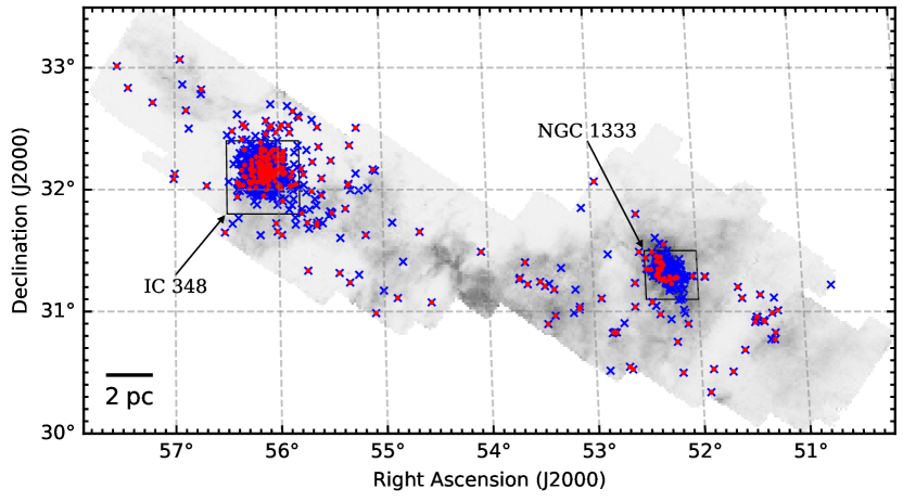
Figure 1: Spatial distribution of the initial YSO sample (blue crosses) overlaid on the FCRAO ¹²CO $J=1\to 0$ integrated intensity map (Ridge et al., 2006). Additional red points mark the 311 sources in our working sample. The two rectangles mark the two young clusters IC 348 and NGC 1333. The scale bar on the lower left shows a size of 2 pc at a distance of 300 pc.

2.2 ZTF Photometry

The Zwicky Transient Facility (ZTF; Kulkarni, 2018) is a time-domain photometric survey currently in progress. It uses a 47 deg² camera consisting of 16 individual CCDs each 6k$\times$6k covering the full focal plane of the Palomar 48-inch (P48) Schmidt Telescope at Palomar Observatory (Masci et al., 2019). In this paper, we analyze data from the thirteenth public ZTF data release (ZTF DR13), which corresponds to more than four years of data taken between 2018 March 17 and 2022 July 8 (58194$\leq$MJD$\leq$59768). The photometry is provided in the $g$, $r$ and $i$ bands, with a uniform exposure time of 30 s in the public survey and is calibrated to the PanSTARRS photometry and reported in AB magnitude. The ZTF DR13 contains about 4.4 billion lightcurves in the $g$, $r$ or $i$ bands, with more than half of them have $\geq$20 epochs of observations. The $r$-band have the most number of lightcurves.

Searching the ZTF archive, we extract $g$-band lightcurves for 466 members and $r$-band lightcurves for 577 members of the Perseus molecular cloud. In this work, we will focus our analysis on the ZTF $g$ and $r$-band lightcurves only, since no $i$-band lightcurve is available for our targets. We ignore observations with catflags=32768 that are affected by clouds or contaminated by the moon. For our analysis, we restrict ourselves to sources with mean magnitudes brighter than 20.8 and 20.6 in the $g$ and $r$-band respectively, over the entire time series. Following the procedure in (H22), we further remove observations taken on MJD days 58786, 58787, 58788, 58789 and 58805, that are part of the ZTF high-cadence experiments (Kupfer et al., 2021) and affect the period search. To alleviate the impact from potential outlier measurements in the lightcurves, we remove measurements 5$\sigma$ away from the median magnitude of the corresponding lightcurve. In some cases, an additional one to three points are found to be nonphysically discrepant and are removed. Finally, only lightcurves (5$\sigma$ clipped) with more than 30 measurements are considered for further analysis. Several sources which are located closely are not resolved by the ZTF are removed. In the current work, we only focus on G to M type members. Our final sample contains 288 sources with both $g$- and $r$-band lightcurves.

2.3 LAMOST Spectroscopy

The Large Sky Area Multi-Object Fiber Spectroscopic Telescope (LAMOST), also called the Guoshoujing Telescope, is a quasi-meridian reflecting Schmidt telescope located at Xinglong Observatory Station in Hebei province, China. The telescope has an effective aperture of $\sim$4 m and a field of view of 5^∘ in diameter. The telescope is equipped with 16 spectrographs and 4000 fibers, each spectrograph has a resolving power of $R\approx 1800$, and the wavelength coverage is 3700$-$9100 Å(Cui et al., 2012; Zhao et al., 2012; Liu et al., 2015; Luo et al., 2015).

Cross matching our working sample with the data release 9 of the LAMOST survey (LAMOST DR9), we obtain LAMOST spectra for 174 members in our working sample. There are 151 sources showing prominent H$\alpha$ emission lines in their LAMOST spectra. The accretion properties of these H$\alpha$ emitters are studied in Section 3.3.

3 Target Properties

3.1 Stellar Masses and Ages

Spectral types and extinction corrections have been provided for the full YSO sample (Luhman et al., 2016; Esplin & Luhman, 2017; Luhman & Hapich, 2020; Kounkel et al., 2019; Wang et al., 2022). We use the same methods as described in Wang et al. (2022) to convert spectral types and observed $J$ magnitudes to effective temperatures and bolometric luminosities, respectively, and then to construct the Hertzsprung-Russell (H-R) diagram (Figure 2). Stellar masses and ages are estimated from their locations on the H-R diagram for individual sources using the PARSEC stellar model (Bressan et al., 2012). In Figure 3, we display the distributions of stellar ages and stellar masses. Though they span a large range of age, most objects in our working sample have ages between 1 to 10 Myr, with median age of 3.8 Myr. More than 90% of the objects in our working sample are less massive than $1\;M_{\odot}$, and the median mass is $0.5\;M_{\odot}$.

3.2 Disk Classification

Most of the objects in the full YSO sample have disk classifications based mainly on Spitzer photometry (Dunham et al., 2015; Luhman et al., 2016; Kounkel et al., 2019). We reclassified 6 of objects as disks based on their very red $K_{S}-W2$ colors (marked with blue squares in Figure 4). One additional object is also reclassified as a disk based on its excess emission at $W4$ and $MP1$ bands (marked with green square in Figure 4). Forty objects in our working sample with no disk classifications from the literature are classified here based on their locations on the $K_{S}-W2$ versus $H-K_{S}$ color-color diagram (Figure 4). Objects with $K_{S}-W2$ colors redder than $0.98\times(H-K_{S})+0.22$ are classified as disks and bluer as diskless (Wang et al., 2022). The dividing line separating disks from diskless YSOs is constructed as following. The locus of objects having disk classifications from literature are compared to the dwarf locus from Pecaut & Mamajek (2013) and reddening vector from Wang & Chen (2019). Visually inspecting the color-color plot indicates that vertically shifting the upper border of the dwarf locus due to reddening redward of 0.15 mag can separate disked YSOs from diskless ones fairly well. Five of these 40 objects are classified as disks, and the remaining as diskless ones. We also note several sources classified as disks in the literature are located at the diskless boundary in Figure 4, because their infrared excess is seen only at wavelengths longer than $W2$.

Our working sample comprises of 109 disk objects and 179 diskless objects. The disk fraction of objects in our working sample is 38%, slightly lower than that of the initial sample (46%). This discrepancy is mainly due to that our working sample is constructed based on the ZTF photometry, which may be biased against low mass or embedded objects and stars with edge-on disks. We note that the disked and diskless objects in our working sample share similar mass ranges, and the majority of both samples are less massive than $1\;M_{\odot}$. The KS-test indicates that the two samples are indistinguishable in terms of spectral types ($p=7\%$).

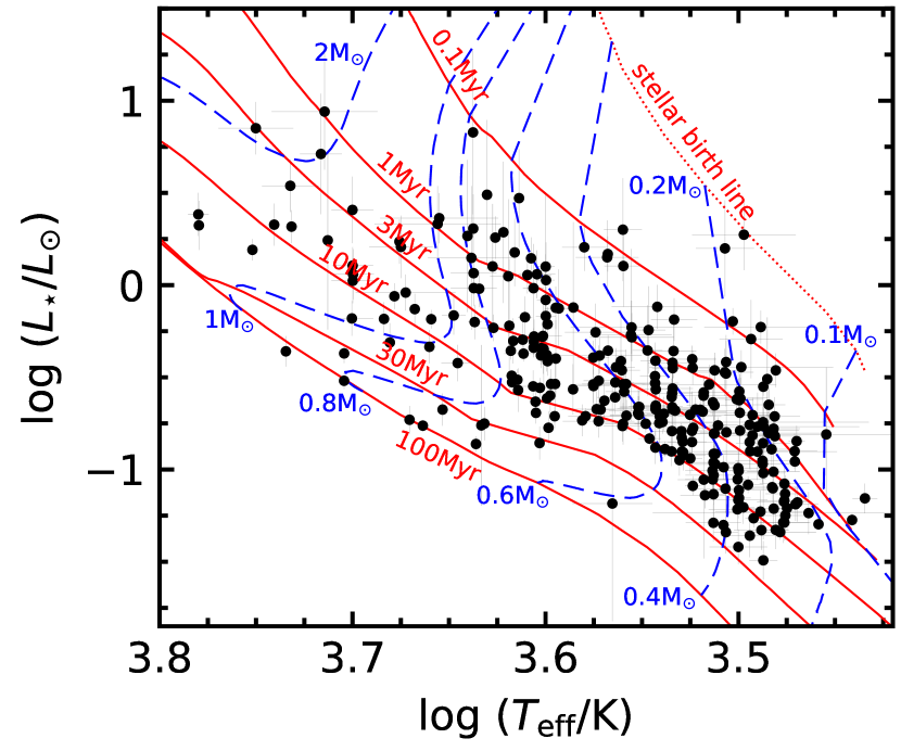
Figure 2: H-R diagram of the objects in our working sample. Overlaid are the isochrones (red solid lines) and mass tracks (blue dashed line) with solar metallicity from the PARSEC stellar model (Bressan et al., 2012), with their corresponding ages and masses indicated. The red dotted line is the stellar birth line.

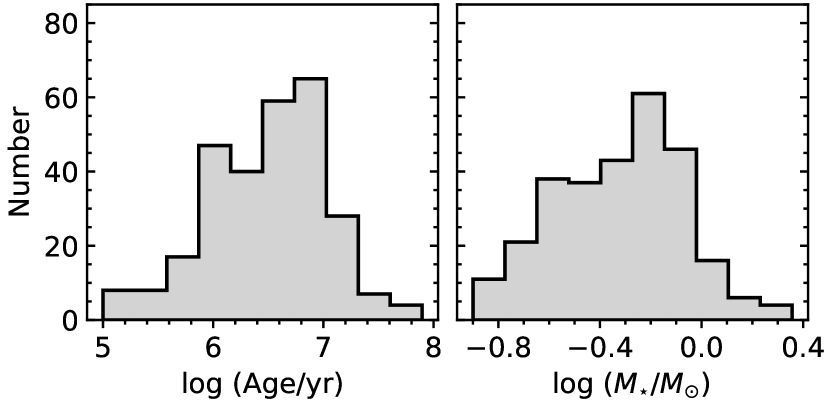
Figure 3: Histograms showing the distribution of stellar ages (left) and stellar masses (right) for the objects in our working sample. These values are estimated using the PARSEC stellar model (Bressan et al., 2012) without correcting the contribution from spots.

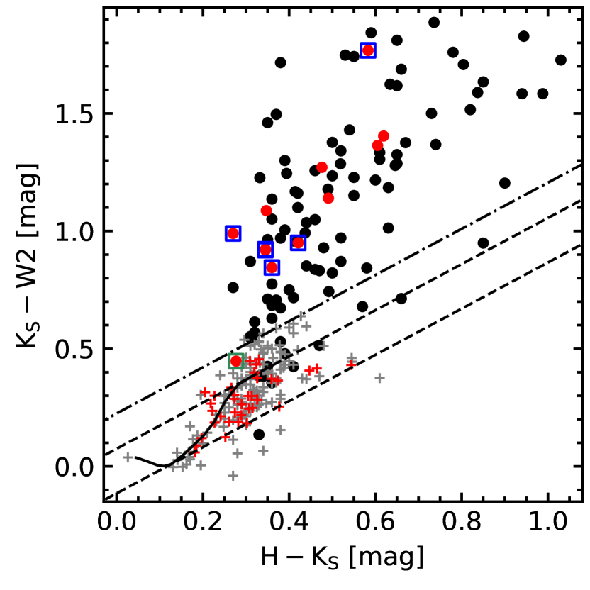
Figure 4: Infrared color-color plot for objects in our working sample. The solid circles and plus signs represent disked and diskless YSOs, respectively. Objects classified by us are highlighted as red. Additional blue and green squares mark sources that are classified as diskless in the literature. The solid curve is the locus of dwarfs from Pecaut & Mamajek (2013), and the dashed lines correspond to the extinction law from Wang & Chen (2019), enclosing the color space of dwarfs due to reddening. The dash-dotted line is the dividing line we use to separate disked YSOs from diskless ones (see Section 3.2 for detail).

3.3 Accretion Properties

Accreting YSOs are generally characterized by strong and broad emission lines in their optical to near-infrared spectra (Hartmann et al., 1994; Muzerolle et al., 1998a, b). Correlations between emission line properties and accretion have been established both theoretically and observationally (e.g., Muzerolle et al., 1998a; Natta et al., 2004; Fang et al., 2009). H$\alpha$ is one of the strongest emission lines in classical T Tauri stars (CTTSs) and has been widely used as an indicator of accretion activity (White & Basri, 2003; Muzerolle et al., 2003; Natta et al., 2004; Fang et al., 2009, 2013).

In this section, we use the H$\alpha$ emission lines to study the accretion activities for a sub-sample of our working sample. We use the equivalent widths of H$\alpha$ emission lines ($\rm EW_{H\alpha}$) to distinguish between CTTSs and weak-line T Tauri stars (WTTSs) for the disk population. Since there are no unique $\rm EW_{H\alpha}$ value to distinguish all CTTSs from WTTSs, due to the “contrast effect” (Basri & Marcy, 1995) and line optical depths (Ingleby et al., 2011), we adopt the spectral type dependent thresholding values from Fang et al. (2009) to distinguish between CTTSs and WTTSs, that is an object is classified as CTTS if $\rm EW_{H\alpha}\geq 3\;\AA$ for K0-K3 stars, $\rm EW_{H\alpha}\geq 5\;\AA$ for K4 stars, $\rm EW_{H\alpha}\geq 7\;\AA$ for K5-K7 stars, $\rm EW_{H\alpha}\geq 9\;\AA$ for M0-M1 stars, $\rm EW_{H\alpha}\geq 11\;\AA$ for M2 stars, $\rm EW_{H\alpha}\geq 15\;\AA$ for M3-M4 stars, $\rm EW_{H\alpha}\geq 18\;\AA$ for M5-M6 stars, $\rm EW_{H\alpha}\geq 20\;\AA$ for M7-M8 stars. We further refine the classification by assigning the diskless objects as WTTSs. Forty sources are classified as CTTSs, and 134 sources are classified as WTTSs. Of the WTTSs, 86% (116/134) are diskless objects.

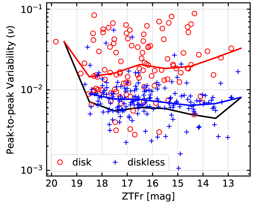
Figure 5: Normalized peak-to-peak variability metric $\nu$ as a function of mean $r$ magnitude for our working sample. Disked and diskless objects are indicated with red circles and blue pluses, respectively. The black solid line is the 15th percentile line, i.e., the boundary line we use to distinguish between variables and non-variables. The red and blue solid lines mark the median trends for disk and diskless populations, respectively.

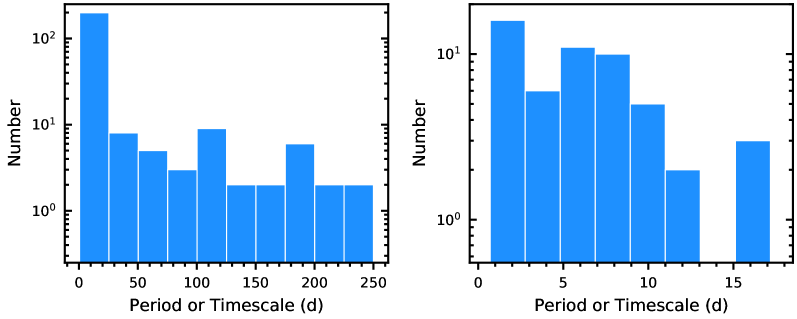
Figure 6: Histograms showing the distribution of periods or timescales of the periodogram peaks. Left panel shows all timescales, and right panel shows only sources classified as periodic variables.

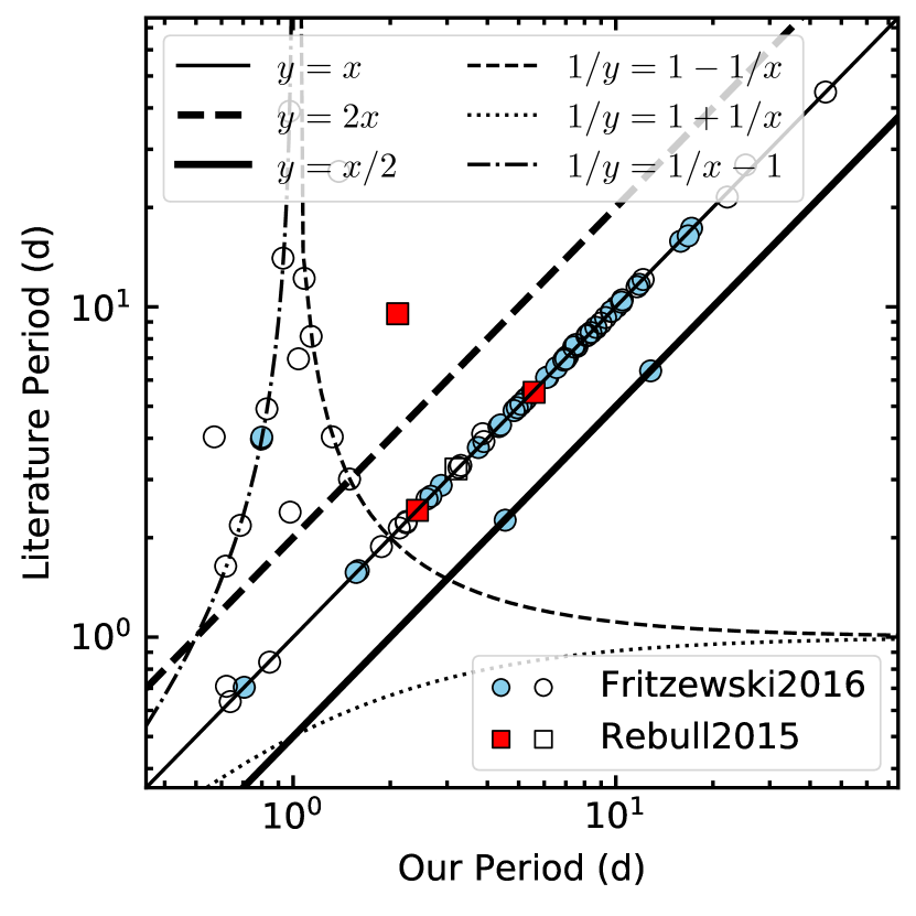
Figure 7: Comparison of periods between our work and previous literature for sources we classified as periodic (filled symbols) or quasiperiodic symmetry (open symbols). Circles are periods from Fritzewski et al. (2016) and squares are periods from Rebull et al. (2015). Different lines indicate the different harmonics and the alias with the $\sim$1 day sampling as shown in the legend. The $x$ in the legend represents our periods and $y$ is literature periods.

4 Lightcurve Analysis

Most objects in our working sample have 200$-$500 observations during the $\sim$4 years ZTF data stream. Since the $r$-band photometry is much better than the $g$-band and the cadence is generally higher in the $r$-band than in the $g$-band, our analysis of the lightcurves in this section is mainly based on the $r$-band photometry. The $g$-band photometry is only used in analyzing the CMD pattern and when mentioned specifically.

4.1 Variability Search

We use the normalized peak-to-peak variability metric (Sokolovsky et al., 2017)

$$\nu=\dfrac{(m_{i}-\sigma_{i})_{\rm max}-(m_{i}+\sigma_{i})_{\rm min}}{(m_{i}-\sigma_{i})_{\rm max}+(m_{i}+\sigma_{i})_{\rm min}},$$ (1)

to measure variability amplitude for objects in our working sample, where $m_{i}$ is a magnitude measurement and $\sigma_{i}$ is the corresponding measurement uncertainty. The maximum and the minimum are determined from the full light curve. The normalized peak-to-peak variability is a sensitive variability indicator (Sokolovsky et al., 2017) since we have removed potential outliers from each light curve (see Section 2.2).

Following H22, we consider an object variable if its $\nu$ metric is greater than the 15th percentile of $\nu$ as a function of mean $r$ magnitude (Figure 5). As pointed out in H22, although this is not a rigorously justified cutoff, this cut ensures that we select the fractionally larger amplitude objects as variables at each brightness level. We select 238 (83% of our working sample) objects as variables based on the $\nu$ metric.

92% of the disk population and 77% of the diskless population are variables. The variability fraction of the disk population is much higher than that of the diskless population, as can be more evidently seen in Figure 5. In addition, the $\nu$ metrics are typically 1-3 times larger for disk population than for diskless population (as indicated with red and blue solid lines in Figure 5).

The properties of the 238 variables are listed in Table LABEL:tab:variables. The variability amplitude listed in the table is calculated as the difference between the 5th and 95th percentile magnitudes.

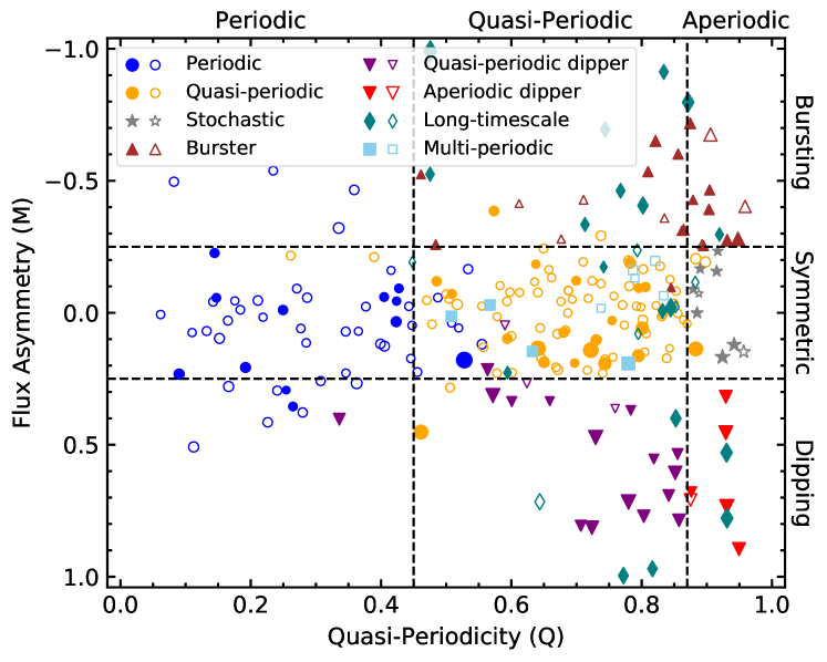
Figure 8: Quasiperiodicity ($Q$) vs. flux asymmetry ($M$) for our sample of variables, color coded by lightcurve morphological types. The sizes of the points are proportional to the square root of the normalized peak-to-peak variability metric $\nu$. Disked objects are indicated with solid symbols and diskless objects are marked with open symbols. Note that unclassifiable variables are not included in this plot, since they fall off the viewing range of the plot.

4.2 Period Search

We use the Astropy (Astropy Collaboration et al., 2013, 2018) implementation of the Lomb-Scargle periodogram (Lomb, 1976; Scargle, 1982; VanderPlas & Ivezić, 2015; VanderPlas, 2018) to compute the periodogram for each variable and search for periods between a minimum period of 0.5 days and a maximum period of 250 days. Periods between 0.5$-$0.51, 0.98$-$1.02, 1.96$-$2.04, and 26$-$30 days are flagged for further analysis to avoid the most common aliases associated with the solar and sidereal days, as well as the lunar cycle (Rodriguez et al., 2017; Ansdell et al., 2018; Hillenbrand et al., 2022). We also reject periods with half or double multiples that fail at least one of the aforementioned alias checks to account for additional potential aliases. In most cases, the period is searched using the $r$-band lightcurves, except for cases where the $g$-band lightcurve is better phased.

We then use the find_peaks function from the PYTHON package scipy (Virtanen et al., 2020) to search for power peaks in the periodogram. Only peaks higher than the 1% false alarm level are considered significant, and are retained for further analysis. If there are no peaks more significant than the 1% false alarm probability, we take the period corresponding to the maximum power of the periodogram as estimates of the variability timescales. In most cases the peak with the maximum power is adopted as the real period, but there are cases where the peak with slightly lower power is adopted as the real for better interpreting the beat patterns and improving the phase dispersion minimization (i.e., with smaller $Q$ values determined in the next section).

For sources with multiple peaks in the periodogram, the frequencies of the peaks are checked for possible alias and beats following the proposals in VanderPlas (2018). The source is labeled as multiperiodic if there are peaks with frequencies that are not alias or beats of the adopted real period. Based on our visual inspection, only the first four highest peaks are checked for sources with more than four peaks in their periodograms.

The distribution of the periods or timescales are displayed in Figure 6. Our variable sample has a relatively flat distribution, extending to more than 200 days. For the periodic objects, our sample is double peaked with a tail toward longer periods. The two peaks at around 1.5 days and one week are consistent with the populations of fast and slow rotators, respectively (Gallet & Bouvier, 2013).

We compare our periods with that from literature (e.g., Fritzewski et al., 2016; Rebull et al., 2015) in Figure 7. In most cases, our periods are consistent with that from literature. The largest discrepancy is found for objects we classified as quasiperiodic, for which we found periods that are aliases of the literature periods with the 1 day sampling.

Table 1: Criteria used to classify the lightcurves into different variability categories.

$Q$	$M$	Variability Type
$Q<0.45$	$-0.25<M<0.25$	Periodic [P]
$0.45<Q<0.87$	$-0.25<M<0.25$	Quasiperiodic Symmetric [QPS]
$0.45<Q<0.87$	$M>0.25$	Quasiperiodic Dipper [QPD]
$Q>0.87$	$M>0.25$	Aperiodic Dipper [APD]
$\cdots\cdots$	$M<-0.25$	Burster [B]
$Q>0.87$	$-0.25<M<0.25$	Stochastic [S]
$Q>1$ or $Q<0$	$\cdots\cdots$	Unclassifiable [U]

4.3 Light-curve Classification

We classify our light-curves into different types based on two statistics quantifying quasiperiodicity ($Q$) and flux asymmetry ($M$), first developed by Cody et al. (2014) based on regularly sampled time series from space-based platforms and further refined by Cody & Hillenbrand (2018). The $Q$ and $M$ metrics are defined as follows,

$$\begin{cases}Q=\dfrac{\sigma_{\rm resd}^{2}-\sigma_{\rm phot}^{2}}{\sigma_{m}^{2}-\sigma_{\rm phot}^{2}}\\[12.91663pt] M=\dfrac{\left<m_{10\%}\right>-m_{\rm med}}{\sigma_{m}}\end{cases},$$ (2)

where $\sigma_{m}$ is the scatter of the original light-curve, $\sigma_{\rm resd}$ is the scatter of the residual light-curve after subtracting the smoothed dominant periodic signal, $\sigma_{\rm phot}$ is taken as the mean photometric error of all observations in an object’s light-curve, scaled by a factor of 1.25 to account for an initial compression of $Q$ values (H22), $m_{\rm med}$ is the median magnitude of the light-curve, and $\left<m_{10\%}\right>$ is the mean magnitude of the top and bottom 10% measurements. The reader is referred to H22 for more details on the $Q$ and $M$ metrics. In most cases, the $Q$ and $M$ metrics are calculated for each variable using the $r$-band lightcurve data. For several cases, the period is determined for the $g$-band lightcurve only, and the $g$-band lightcurve is used to determine these statistics. The variables in our working sample are classified into 9 categories, based on their locations in the $Q-M$ plane (Figure 8) and additional visual inspection.

Since the time series data analyzed here is from the same instrument as in H22, we adopt the same boundary values of $Q$ and $M$ metrics as H22. The boundary values used to classify the lightcurves into different variability categories are summarized and listed in Table 1. In addition to the seven categories listed in Table 1, we classify objects with variability timescales larger than 100 day as long timescale (L) variables, and objects having more than one periods are classified as multi-periodic (MP) variables. All of the lightcurves and corresponding periodograms are visually inspected. In most cases, the $Q$ and $M$ classifications are consistent with our visual inspection. For 40 cases (labeled in Table LABEL:tab:variables), we adjust their type to favor our visual classification. We note that the original classification scheme does not involve the $Q-M$ plane with $0<Q<0.45$ and $M>0.25$. About 10 of these cases have $(Q,\;M)$ values in this region, and these sources are classified as periodic variables based on their well phased lightcurves. Other adjustments mainly occur around the boundaries, and the most common adjustment is from quasiperiodic symmetric category to periodic type for seven objects due to their well-phased lightcurves and their quite clean periodograms. These adjustment does not affect our statistics significantly. We should mention that both the photometric precision and the cadence will affect the measurement of the $Q$ metric, and thus the classification of the lightcurve morphology. The readers are referred to H22 for a discussion on these effects (see their Appendix C).

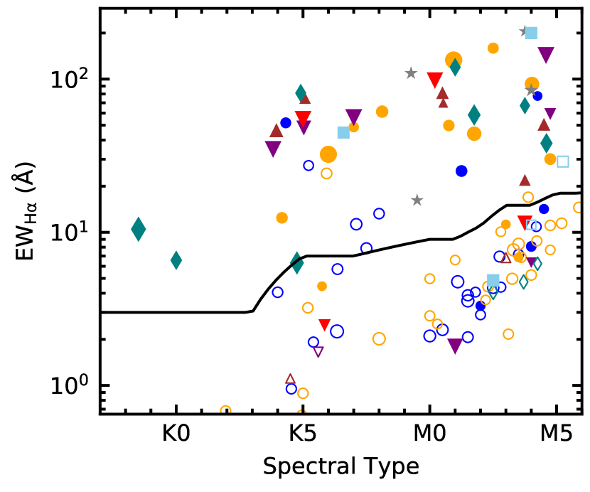
Figure 9: Equivalent width of H$\alpha$ emission line as a function of spectral type. The symbols are the same as in Figure 8. The solid line is the dividing line separating CTTSs from WTTSs (Fang et al., 2009).

Table 2: Distribution of lightcurve morphological category for objects in our variable sample.

Variability Type	Numbers			Numbers
	disk	diskless	total	CTTS	WTTS	total
Periodic [P]	12	41	53	3	28	31
Quasiperiodic Symmetric [QPS]	22	71	93	10	58	68
Multi-periodic [MP]	4	5	9	2	4	6
Stochastic [S]	7	2	9	4	1	5
Burster [B]	15	7	22	6	2	8
Quasiperiodic Dipper [QPD]	16	3	19	5	6	11
Aperiodic Dipper [APD]	5	1	6	2	2	4
Long Timescale [L]	18	6	24	7	5	12
Unclassifiable [U]	0	2	2	0	1	1
Total number	100	138	238	39	107	146

Figure 10: An example displays constructing the phase series CMD for the source 2MASS J03442812+3216002. Panel (a): The $g$-band phase-folded lightcurve is displayed as small points with error bars. The blue squares show the median magnitudes in individual phase bins, and the horizontal error bars are the corresponding phase bins. The standard deviations of the median magnitudes are smaller than the symbol size. Panel (b): Similar as panel (a), but for the $r$-band data. Panel (c): The phase series CMD is displayed as blue points. The black line is the straight line from the orthogonal regression. The error bar in the lower left displays the typical uncertainty of the data points. The corresponding CMD slope angle is labeled. Panel (d): Similar as panel (c), but displaying the time series CMD for comparison.

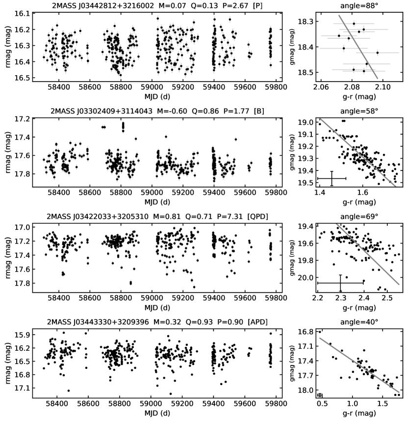
Figure 11: Examples showing the lightcurves (left panels) and corresponding CMDs (right panels) for periodic, burster, quasiperiodic dipper and aperiodic dipper categories. In the left panels, the source name, the flux asymmetry ($M$), the quasiperiodicity ($Q$), the period/timescale and the lightcurve classification are labeled for each source. In the right panels, the gray lines are the straight line from the orthogonal regression, and the corresponding CMD slope angles are labeled.

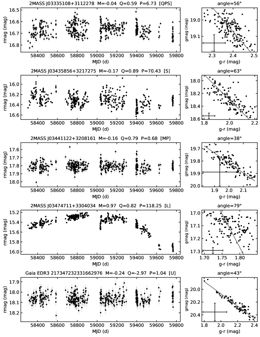
Figure 12: Same as Figure 11, but for quasiperiodic symmetric, stochastic, multi-periodic, long timescale and unclassifiable categories.

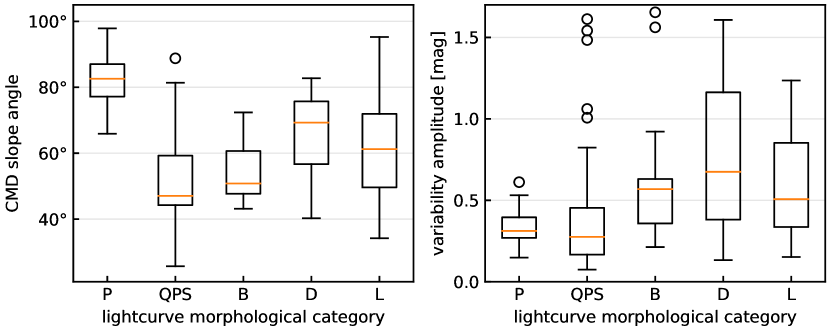
Figure 13: Boxplots showing the distributions of CMD slope angle (left) and variability amplitude (right) for different lightcurve morphological categories. Multi-periodic and unclassifiable categories are not included here.

The numbers of different lightcurve morphologies are listed in Table 2. The dominant lightcurve morphology in our variable sample is quasiperiodic symmetric. For the disk population, dipper (both quasiperiodic dippers and aperiodic dippers), burster, stochastic and long timescale categories are also common. We performed two-dimensional Kolmogorov-Smirnov (KS) test (Peacock, 1983) to compare the 2D parameter space ($Q$, $M$) for disk and diskless populations. We found $p$-value of $2\times 10^{-4}$ corresponding to the null-hypothesis that disk and diskless populations occupy the same ($Q$, $M$) space. The disk population is dominated by asymmetric and non-repeatable lightcurves, while the diskless population is dominated by symmetric and repeatable lightcurves. There are eleven diskless objects classified as bursters or dippers. Visually inspecting their lightcurves indicates that they have variability amplitudes comparable to the measurement uncertainties or their $M$ metrics are affected by several photometric measurements, which makes their classifications unreliable. As pointed out in Section 3.2, the disk and diskless populations in our working sample share similar mass ranges and spectral type distributions. In addition, we don’t find any trends of variability properties as functions of stellar masses or spectral types. Considering these issues together, the differences of the variability patterns of the two populations are dominated by the presence or absence of disks.

The $\rm EW_{H\alpha}$ value are displayed as a function of spectral type and lightcurve morphological category in Figure 9 for a sub-sample of 146 variables having LAMOST spectra. In the figure, nearly all sources in the burster (brown upward triangles) and stochastic (gray star symbols) categories are CTTSs. Half of the dippers and long timescale variables are also CTTSs. More than 85% (90/105) of variables classified as P, QPS, or MP are WTTSs. The numbers of different lightcurve types in this sub-sample are listed in Table 2. These are consistent with the results on the different properties of the disked or diskless variables discussed above.

4.4 CMD Analysis

There are many different physical mechanisms that can drive the photometric variability observed in young stars (see H22 for a summary of the mechanisms related to different lightcurve morphologies). Color time series data is a powerful tool in distinguishing these physical mechanisms. Our working sample is constructed to have both $g$ and $r$-band lightcurves, so it is possible for us to analyse $g-r$ color times series data, besides $g$ or $r$-band lightcurves.

Since the ZTF $g$ and $r$-band observations are not simultaneous, with time steps of a few hours up to a few days, we construct the CMDs with the following two methods.

The first method (Method 1) is the same as that in H22. For each source, the $r$-band lightcurve is trimmed into the corresponding $g$-band time span. For each time point in the trimmed $r$-band lightcurve, we search the $g$-band lightcurve for paired observations with one just before this time and another after this time, we then linearly interpolate the paired $g$-band observations to this time point and to estimate the $g-r$ colors, if the time interval of the paired $g$-band observations is less than 3 days. The errors of the interpolated $g$ magnitudes and $g-r$ colors are estimated using the PYTHON package uncertainties (Lebigot, 2010).

The second method (Method 2) we developed to construct the CMD is based on the phase-folded lightcurves and applied to only periodic objects in our sample. For periodic objects, both the $g$ and $r$-band lightcurves are phase-folded at the adopted periods. The median magnitudes, the standard deviations and the number counts are determined for 10 evenly spaced phase bins, for both the $g$ and $r$-band lightcurves, for each source. The errors of the magnitudes corresponding to each phase bin is estimated as the standard deviation divided by the square root of the number count, of that phase bin. The $g-r$ colors are estimated at the same phase, with the errors estimated using the uncertainties package as well. The CMD constructed this way will be designated the phase series CMD in the remaining of the paper. An example of constructing the phases series CMD is displayed in Figure 10.

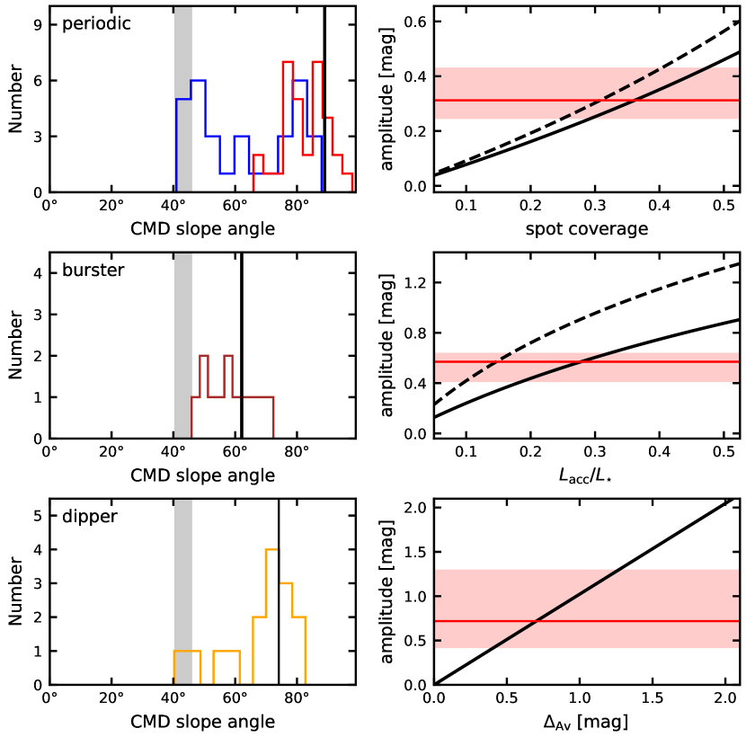
Figure 14: Left panels: histograms showing the distributions of CMD slope angles for periodic, burster and dipper variables from top to bottom, as labeled in the corresponding panels. The gray shaded area display the $1\sigma$ range of the slope angles for non-variables in our sample (see the discussion in Appendix A). The vertical line in each panel corresponds to the angles due to changes in spot coverage, variable accretion and variable extinction, respectively, from top to bottom. The vertical lines in the left top and middle panels are calculated for $T_{\rm eff}=4000\;\rm K$. The blue and red histograms in the left top panel represent the angles determined using Method 1 and Method 2, respectively. Right panels: the variability amplitudes observed are compared to that due to changes of spot coverage, variable extinction and variable accretion for periodic, burster and dipper variables, respectively, from top to bottom. The red horizontal line and the shaded area in each panel show the median value and the $1\sigma$ range of the amplitude for the corresponding sample, respectively. The solid and dashed lines in the right top and middle panels correspond to calculations for $T_{\rm eff}=4000\;\rm K$ and 3500 K, respectively.

For each source in the variable sample, we fit a straight line to its time/phase series CMD using an orthogonal distance regression in the PYTHON package scipy.odr (Virtanen et al., 2020), following (Poppenhaeger et al., 2015; Hillenbrand et al., 2022). This method is chosen to account for the significant and partially correlated errors in both axes. For the CMD constructed using the first method, only the central 95% of the CMD spans in $g$ and $g-r$ are included in the regression, to alleviate the effect of outliers.

The slope angles are defined as the inverse tangent of the best-fitting slopes in the $g$ versus $g-r$ CMDs. The slope angles are expressed in degrees and span from $0^{\circ}$ (corresponding to color changes with no associated $g$-band variability) to $90^{\circ}$ (corresponding to $g$-band variability with no color changes). To estimate the errors on the best-fitting slope angles, the CMD points are perturbed according to the errors in $g$ magnitudes and $g-r$ colors assuming Gaussian errors (this is similar to the perturbation method described in Curran (2014)) and the orthogonal distance regression is performed on the perturbed points. This procedure is repeated 1000 times for each source and the errors on the angles are estimated as the standard deviation of the 1000 realizations. Only sources with errors less than $10^{\circ}$ are considered for further analysis. This error estimation is slightly different from that in H22, where the errors are estimated using a bootstrap technique. Several examples of the constructed CMDs and corresponding lightcurves are displayed in Figure 11 and 12.

In Figure 13, we display the distribution of CMD slope angle and variability amplitude for different lightcurve morphological categories. Strictly periodic objects show the largest angles, and bursters have much flatter slopes than dippers. Periodic and quasiperiodic sources have the lowest variability amplitudes. In the next section, we demonstrate that the angles of periodic variables are consistent with the spot model, the angles of bursters are consistent with the accretion model, and the angles of dippers are consistent with variable extinction. We also note that stochastic variables have angles in consistent with variable accretion, which may indicate that these sources are ongoing accretion activity as well (as demonstrated in Stauffer et al., 2016). All but one of the stochastic variables having LAMOST spectra are accreting stars.

5 Discussion

In Section 4.3 we classified our variables into different categories and, in Section 4.4 we analysed the CMD patterns using orthogonal distance regression technique on $g-r$ versus $g$ CMD. In this section, we will discuss the different CMD patterns of periodic, burster and dipper categories, and relate them with specific mechanisms.

There are 53 ($\sim$21% of the variable sample) objects classified as strictly periodic variables, with CMD slope angles determined for 32 of them using Method 1 and Method 2. As shown in the upper left panel of Figure 14, we obtain much larger angles using Method 2 than using Method 1. These periodic variables are generally explained as stellar rotation modulated by star spots on the stellar surface. We model the CMD pattern for a star with $T_{\rm eff}=4000\;\rm K$ and a cool spot 500 K cooler than the effective temperature on the stellar surface. The CMD trend arising from the cool spot is nearly vertical, corresponding to colorless variability with associated changes in $g$ magnitudes and the corresponding slope angle is essentially 90^∘. Gully-Santiago et al. (2017) also found nearly colorless changes in $B-V$ or $V-R$ colors with associated brightness changes in $V$-band. Changing the effective temperatures and the temperature contrasts does not alter the angles significantly.

Comparing the slope angles we determined with this simple model, we find that the angles from Method 2 are more consistent than from Method 1 with the cool spot model. One possible reason could be that the interpolation of the $g$-band observations to the $r$-band observing time in Method 1 introduce additional uncertainties, especially for fast rotators. We do note a trend of decreasing differences between the two methods with increasing period. The effect of noise on the CMD pattern is discussed in Appendix A. We also compared the variability amplitude in $g$-band with the cool spot models (upper right panel of Figure 14). The comparison indicates that the typical changes in spot coverage of our periodic variables is in the range 30% to 40%, and this range is consistent with the cool spot coverage in Cao & Pinsonneault (2022); Herbert et al. (2023). For our analysis, we model a single spot on the stellar surface, and the reader is referred to Guo et al. (2018) for a discussion about multiple spots configuration. In addition, the spot coverage estimated from lightcurve amplitude alone may be underestimated (Rackham et al., 2018).

Among the sample of variables with disks, 15 ($\sim$15% of the sample) are bursters, and 12 of the 15 have CMD slope. Burster variables are thought to arise from discrete accretion shocks. We model the CMD pattern for a star with $T_{\rm eff}=4000\;\rm K$, and adopt the accretion spectrum from Manara et al. (2013) with the same model parameters as in Flaischlen et al. (2022), i.e., the electron temperature $T_{\rm slab}=11000\;\rm K$, the electron density $n_{\rm e}=10^{15}\;\rm cm^{-3}$, and the optical depth at $300\;\rm nm$ $\tau_{300}=5.0$. The CMD slope angles due accretion variation is around $62^{\circ}$, in consistence with the bursters in our sample (middle left panel of Figure 14). We also compared the variability amplitudes in $g$-band with the accretion model (middle right panel of Figure 14), and the comparison indicate that the bursters in our sample have changes of $L_{\rm acc}/L_{\star}$ in the range 0.1 to 0.3, these values are larger than the typical value of 0.11 in Flaischlen et al. (2022), but within 1$\sigma$ range of that work.

Among the sample of variables having disks, there are 21 ($\sim$21% of the sample) dippers, with CMD slope angles determined for 15 of them. The slope angles of these dippers are $\sim$74.1^∘, consistent with that expected from interstellar extinction according to the extinction law from Schlafly & Finkbeiner (2011) with total to selective extinction ratio of $R_{V}=3.1$. Comparing the variability amplitudes in $g$-band with that due to extinction changes (bottom right panel of Figure 14), we find that most of the dippers have variable extinction with $A_{V}$ changes in the range of $0.5-1.3$ mag.

In this section, we have related periodic, burster and dipper categories with spot modulated stellar rotation, variable accretion and extinction changes, respectively. But we should keep in mind that multiple physical processes are taking place in the young star systems, making the above calculations being over simplified. For example, Rackham et al. (2018) pointed out that the spot coverage may be underestimated from lightcurve amplitude alone. Additional high quality observations should be helpful to decouple these physical processes, and to determine the corresponding physical parameters more accurately.

Since YSOs are generally found to be more variable than field stars, time series photometry is powerful in selecting candidate samples dominated by YSOs. Future and existing time-domain surveys, such as the ZTF (Kulkarni, 2018) and the Vera C. Rubin Observatory (Large Synoptic Survey Telescope; Ivezić et al., 2019; Bianco et al., 2022), will help search the fainest YSOs that are invisible to astrometry surveys, such as the Gaia (Gaia Collaboration et al., 2016), as well as further improve our knowledge about the mechanisms related to different variability behavior.

6 Summary

In this work we studied the variability of 288 YSOs in the Perseus molecular cloud using the about 4 years time series data from the ZTF. The main results are summarized as follows.

1. We identified 238 sources as variables based on the normalized peak-to-peak variability metric. We found variability fractions of 83% for the whole working sample, 92% for the disk population, and 77% for the diskless population. Disked YSOs are more variable than diskless YSOs.

2. The variables are classified into 9 morphological categories mainly based the flux asymmetry ($M$) and quasiperiodicity ($Q$) metrics. The dominant variability behavior of these variables are strictly periodic (21.3% of the variable sample) and quasiperiodic (39.1% of the variable sample) variables. But for the disk population, the burster, dipper, long timescale and stochastic categories are also common.

3. We analyze CMD pattern of the variables using quasi-simultaneous multiband photometry from the ZTF. We found that periodic variables have the steepest CMD pattern, and that bursters have much flatter slopes than dippers. Periodic and quasiperiodic variables have the lowest variability amplitudes. The periodic variability is consistent with spot modulated stellar rotation, with spot coverage changes of 30% to 40%. The burster variability is consistent with accretion induced brightness changes, with accretion luminosity changes in the range of $L_{\rm acc}/L_{\star}=0.1-0.3$. The dipper variability is consistent with variable extinction with $A_{V}$ changes in the range of $0.5-1.5\;\rm mag$.

Appendix A CMD Pattern Due to Noise

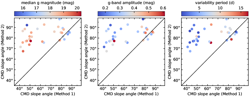
Figure 15: Comparison of CMD slope angles determined using Method 1 and Method 2 for periodic variables in our sample. The symbols are color coded according to the median $g$ magnitude (left), the variability amplitude in $g$-band (middle) and the variability period (right). The straight line in each panel represents the line of equality.

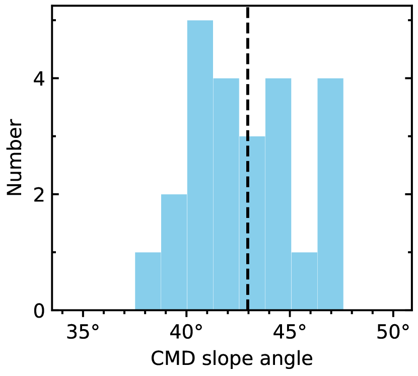
Figure 16: Histogram showing the distribution of CMD slope angles determined using Method 1 for non-variables in our sample. The black vertical line corresponds to the angle of 43^∘ for the typical uncertainties of our sample.

In Section 5, we note that the CMD slope angles determined using Method 1 for periodic variables deviate significantly from that of spot induced variability, while that from Method 2 is consistent with the model. This discrepancy could be attributed to the noise and the interpolation method. We compare the two angles in Figure 15, and note trends of decreasing discrepancies between the two angles with increasing brightness, variability amplitudes and variability period. In Figure 16, we display the CMD slope angles determined using Method 1 for those non-variables, whose CMD pattern should be dominated by the uncertainties in the measurements or introduced during the interpolation for $g$-band photometry. Those non-variables have angles in the range 40^∘ to 45^∘, in consistent with the peak around 40^∘ of the blue histogram in the upper left panel of Figure 14. In fact, given the typical photometric uncertainties of our sample, 0.06 mag in $g$-band and 0.02 mag in $r$-band, a random sampling in the photometry can lead to a CMD slope angle of $\sim$43^∘. Some dippers also have CMD slope angles close to $\sim$43^∘ in Figure 14. These sources generally have variability amplitude comparable to the measurement uncertainties and the measurements of their CMD slope angles could be affected by the noise discussed above.

Appendix B Table List the Properties of Variable

Table 3: Properties of Variables in the Perseus Molecular Cloud

Identifier	R.A.	Decl.	SPT	Diska	CTTSb	$\left<r\right>$	$\nu$	Amplitude	Timescale	$Q$	$M$	Category	Angle
	(deg)	(deg)				(mag)		(mag)	(day)				(deg)
Gaia EDR3 124009935063344128	51.245429	31.010398	M3.1	N	N	16.12	0.0078	0.19	50.36	0.81	0.08	QPS	68.7
Gaia EDR3 123994679339516800	51.281136	30.828328	M2.8	N	N	16.59	0.0065	0.18	3.18	0.85	-0.04	QPS	41.0
2MASS J03250943+3046215	51.289291	30.772661	K9.3	Y	Y	18.12	0.0299	0.96	8.31	0.92	-0.16	S	62.1
Gaia EDR3 123998252752298752	51.302425	30.989481	K9.5	Y	Y	13.29	0.0250	0.31	11.90	0.88	-0.09	S	50.9
Gaia EDR3 123996874066752640	51.379737	30.918846	M5.2	N	N	17.62	0.0090	0.33	34.59	0.65	-0.24	QPS	44.9
2MASS J03253315+3055443	51.388165	30.928993	M0.9	Y	Y	15.74	0.0701	1.61	4.78	0.72	0.14	QPS	68.2
Gaia EDR3 124018318839496064	51.407963	31.139139	M0.2	Y	Y	15.61	0.0576	1.10	0.86	0.93	0.45	APD	78.0
Gaia EDR3 123999936379477504	51.445275	30.955693	M4.6	Y	Y	16.83	0.0353	0.86	121.39	0.85	0.40	L	71.9
2MASS J03254886+3057258	51.453590	30.957169	K4.5	Y	$\cdots$	14.58	0.0516	1.03	143.26	0.93	0.53	L	34.2
2MASS J03255275+3054490	51.469818	30.913614	K5.8	Y	N	15.05	0.0184	0.28	1.17	0.88	0.68	APD	79.1
Gaia EDR3 124002856957227648	51.582532	31.110303	K7	Y	N	16.09	0.0351	0.72	9.68	0.80	0.77	QPD	77.4
Gaia EDR3 124030138589484672	51.617565	31.202155	K7	Y	Y	14.47	0.0653	1.24	5.76	0.78	0.72	QPD	78.1
2MASS J03274148+3020166	51.922852	30.337971	K8.1	Y	Y	14.61	0.0185	0.38	3.15	0.65	0.19	QPS	72.9
Gaia EDR3 124034399197073024	51.926947	31.285487	M2.8	N	N	16.23	0.0074	0.24	9.61	0.06	0.01	P	$\cdots$
Gaia EDR3 124034399197072896	51.930860	31.288977	K4.5	N	N	14.36	0.0054	0.15	0.82	0.61	-0.41	B	$\cdots$
2MASS J03282578+3054000	52.107437	30.900009	K2.9	N	N	13.61	0.0059	0.07	45.82	0.77	0.05	QPS	38.8
2MASS J03284242+3029530	52.176777	30.498074	M4.5	Y	Y	16.24	0.0209	0.61	5.83	0.82	-0.65	B	68.7
2MASS J03284618+3116385	52.192458	31.277389	M4.5	Y	$\cdots$	14.93	0.0125	0.21	3.64	0.57	-0.39	QPS∗	70.0
2MASS J03284782+3116552	52.199250	31.282000	M6.5	Y	$\cdots$	18.36	0.0502	1.65	3.79	0.95	-0.28	B	72.4
2MASS J03285105+3116324	52.212750	31.275694	M5	Y	$\cdots$	17.89	0.0177	0.46	115.82	0.77	-0.46	L	61.2
2MASS J03285217+3045055	52.217407	30.751539	K4	Y	$\cdots$	12.88	0.0327	0.44	8.16	0.56	0.22	QPD∗	82.7
2MASS J03285290+3116264	52.220417	31.274056	M5	Y	$\cdots$	18.18	0.0145	0.48	211.66	0.71	-0.33	L	55.8
2MASS J03290031+3113385	52.251292	31.227389	M3	N	$\cdots$	17.82	0.0123	0.45	3.20	0.67	0.22	QPS	44.2
2MASS J03290289+3116010	52.262043	31.266953	K6.2	N	N	15.52	0.0059	0.11	5.20	0.74	-0.02	MP	41.8
2MASS J03290406+3117075	52.266917	31.285417	M5.8	N	$\cdots$	18.02	0.0082	0.33	91.31	0.71	-0.43	B	44.4
2MASS J03291243+3114565	52.301804	31.249033	K2.4	N	N	14.31	0.0051	0.08	1.03	0.84	0.13	QPS	41.8
2MASS J03291465+3133009	52.311069	31.550257	K4	N	N	14.85	0.0083	0.16	5.63	0.58	0.23	QPS	81.1
2MASS J03291766+3122451	52.323583	31.379194	M4	Y	$\cdots$	13.59	0.0153	0.32	5.58	0.42	0.03	P	$\cdots$
2MASS J03291872+3123254	52.328042	31.390389	M2.5	Y	N	14.59	0.0182	0.53	0.90	0.51	0.01	MP	$\cdots$
2MASS J03292187+3115363	52.341125	31.260083	K4	Y	$\cdots$	14.34	0.0883	2.84	2.11	0.53	0.18	P∗	65.9
2MASS J03292314+3120303	52.346458	31.341778	M4.8	Y	Y	16.59	0.0153	0.42	0.72	0.60	0.34	QPD	$\cdots$
2MASS J03292349+3123309	52.347917	31.391944	M3.5	N	N	17.34	0.0077	0.31	1.23	0.29	0.11	P	$\cdots$
2MASS J03292591+3126401	52.358000	31.444472	G8.5	Y	Y	15.24	0.0811	2.20	119.91	0.48	-0.99	L	$\cdots$
2MASS J03292681+3126475	52.361708	31.446528	M2	Y	N	14.10	0.0083	0.21	1.35	0.26	0.35	P∗	$\cdots$
2MASS J03292815+3116285	52.367333	31.274611	M7.5	N	$\cdots$	18.47	0.0201	0.61	2.43	0.33	-0.32	P∗	77.2
2MASS J03292889+3058418	52.370375	30.978278	M4.8	Y	$\cdots$	16.95	0.0122	0.24	1.49	0.78	0.37	QPD	58.6
2MASS J03293038+3119034	52.376625	31.317639	M4.2	Y	Y	15.86	0.0068	0.20	8.77	0.42	-0.04	P	$\cdots$
2MASS J03293255+3124370	52.385667	31.410278	M4.5	Y	$\cdots$	17.95	0.0565	1.46	2.52	0.46	0.45	QPS∗	$\cdots$
2MASS J03293286+3127126	52.386958	31.453528	M4	Y	N	17.43	0.0095	0.31	2.69	0.66	0.33	QPD	$\cdots$
2MASS J03294592+3104406S	52.441750	31.077500	M1	Y	$\cdots$	16.37	0.0174	0.44	0.53	0.90	-0.39	B	57.4
2MASS J03295403+3120529	52.475125	31.348056	M4	Y	Y	15.64	0.0176	0.50	3.13	0.57	-0.03	MP	$\cdots$
2MASS J03301614+3147595	52.567284	31.799868	K6.3	N	N	14.86	0.0208	0.52	1.33	0.36	0.27	P∗	85.9
2MASS J03302409+3114043	52.600375	31.234556	M5	Y	$\cdots$	17.68	0.0163	0.50	1.77	0.86	-0.60	B	58.0
2MASS J03302598+3102179	52.608253	31.038307	K4.5	N	N	13.61	0.0080	0.17	2.23	0.28	0.06	P	92.2
2MASS J03303697+3031276	52.654041	30.524345	K4.8	Y	N	17.74	0.0589	1.24	173.10	0.93	0.78	L	71.4
2MASS J03304399+3032469	52.683304	30.546379	K5.3	Y	$\cdots$	14.47	0.0204	0.47	1.45	0.92	-0.23	S	63.6
2MASS J03311069+3049405	52.794563	30.827942	M4	Y	Y	16.17	0.0342	1.01	7.17	0.80	0.06	QPS	70.0
2MASS J03311471+3049554	52.811291	30.832075	K4.2	Y	Y	16.53	0.0140	0.33	6.76	0.79	0.16	QPS	88.8
2MASS J03311830+3049395	52.826286	30.827658	K3.8	Y	Y	14.61	0.0601	1.07	39.96	0.57	0.31	QPD	$\cdots$
2MASS J03314240+3106249	52.926704	31.106930	K6.6	Y	Y	17.29	0.0166	0.65	0.94	0.63	0.15	MP	$\cdots$
2MASS J03323300+3102216	53.137524	31.039352	M4.6	Y	Y	17.05	0.0636	1.32	5.15	0.73	0.47	QPD	74.0
2MASS J03323405+3100557	53.141911	31.015488	K5.1	Y	Y	15.53	0.0132	0.32	0.57	0.89	-0.25	B	61.5
Gaia EDR3 121147871936317184	53.372048	30.966361	K4	N	N	16.87	0.0065	0.28	3.07	0.66	-0.16	QPS	46.8
2MASS J03333041+3110504	53.376736	31.180670	K4	Y	Y	13.82	0.0301	0.64	1.03	0.93	-0.27	B	64.4
2MASS J03334692+3053500	53.445538	30.897247	M7.1	Y	$\cdots$	18.23	0.0152	0.53	2.07	0.90	-0.47	B	49.9
2MASS J03335108+3112278	53.462856	31.207733	M3.9	N	N	16.67	0.0082	0.28	6.73	0.59	-0.04	QPS	56.2
2MASS J03340166+3114396	53.506939	31.244354	M0.5	Y	Y	15.37	0.0074	0.22	0.73	0.85	-0.10	B∗	56.0
2MASS J03343079+3113243	53.628304	31.223419	M4	Y	$\cdots$	18.23	0.0104	0.57	1.47	0.81	-0.10	QPS	45.8
2MASS J03344987+3115498	53.707813	31.263859	K5.8	Y	N	14.04	0.0070	0.14	1.66	0.75	0.03	QPS	46.0
Gaia EDR3 120460024334304128	54.553027	31.074960	M3.7	N	N	16.59	0.0078	0.19	123.44	0.88	-0.12	L	49.6
Gaia EDR3 217317549813446656	54.650193	31.653468	M1.8	N	N	15.35	0.0068	0.15	5.86	0.51	0.04	P∗	97.9
Gaia EDR3 120463116710737920	54.875402	31.110591	M4.2	N	N	17.12	0.0068	0.23	0.73	0.22	0.02	P	85.2
2MASS J03404040+3137379	55.168335	31.627199	M5.9	N	N	17.97	0.0093	0.42	73.80	0.64	-0.08	QPS	48.3
Gaia EDR3 217510376665297152	55.243254	32.506634	K5	N	N	13.91	0.0085	0.14	1.46	0.64	0.06	QPS	57.3
Gaia EDR3 217458493460476928	55.310242	32.362894	M1.1	N	N	16.56	0.0162	0.48	8.64	0.11	0.51	P∗	88.1
Gaia EDR3 217347232331662976	55.324826	32.047493	M3.5	N	N	18.06	0.0067	0.52	1.04	-2.97	-0.24	U	43.9
Gaia EDR3 216527894305651840	55.328058	31.237570	M2.3	N	N	16.02	0.0096	0.18	7.09	0.83	-0.18	QPS	64.4
2MASS J03411921+3202037	55.330048	32.034370	K9.2	N	$\cdots$	17.84	0.0379	0.91	1.20	0.88	0.71	APD	60.4
Gaia EDR3 216585721745264896	55.360264	31.843630	K7	N	N	16.32	0.0078	0.28	2.91	0.68	0.07	QPS	44.7
2MASS J03414251+3118567	55.427162	31.315769	K2.5	N	N	13.30	0.0120	0.13	2.94	0.62	0.27	QPD	61.1
2MASS J03415745+3148365	55.489384	31.810162	K4.3	Y	Y	15.93	0.0112	0.32	2.24	0.25	-0.01	P	81.2
Gaia EDR3 217444440327486848	55.492348	32.238318	G6	N	N	13.50	0.0055	0.15	3.87	0.64	-0.12	QPS	62.8
2MASS J03422033+3205310	55.584732	32.091949	K7.4	Y	$\cdots$	17.25	0.0225	0.67	7.31	0.71	0.81	QPD	69.3
Gaia EDR3 216590016712558080	55.588347	31.953305	M2.5	N	N	17.25	0.0110	0.47	71.53	0.79	-0.24	L∗	50.1
2MASS J03422585+3221022	55.607746	32.350624	K6	N	$\cdots$	17.05	0.0061	0.28	17.17	0.42	-0.16	P	$\cdots$
2MASS J03422824+3230479	55.617699	32.513313	K7.1	N	N	16.99	0.0122	0.42	4.34	0.23	0.41	P∗	77.9
2MASS J03423219+3143382	55.634144	31.727291	K4.1	N	N	17.27	0.0083	0.58	1.08	0.74	-0.11	QPS	46.9
2MASS J03423291+3142205	55.637157	31.705711	K5	Y	Y	17.54	0.0376	0.79	0.98	0.86	0.79	QPD	54.7
2MASS J03424360+3159150	55.681702	31.987524	K2	N	N	15.28	0.0080	0.18	0.69	0.77	-0.03	QPS	45.7
2MASS J03425467+3143452	55.727802	31.729233	G3.8	N	N	14.38	0.0057	0.13	0.87	0.76	-0.06	QPS	56.0
2MASS J03430214+3207276	55.758949	32.124344	M4.2	N	N	17.58	0.0078	0.38	18.28	0.85	-0.08	QPS	40.6
2MASS J03430679+3148204	55.778292	31.805694	M3	Y	N	17.26	0.0067	0.46	6.10	0.64	-0.18	QPS	43.2
2MASS J03430704+3210182	55.779369	32.171745	K6.2	N	N	16.60	0.0074	0.24	6.16	0.45	0.05	P	$\cdots$
2MASS J03431065+3235323	55.794384	32.592319	K5.9	N	N	16.87	0.0096	0.33	5.89	0.51	0.28	QPS∗	68.0
2MASS J03432438+3238316	55.851612	32.642117	K5.9	N	N	16.46	0.0063	0.28	1.32	0.37	0.07	P	75.8
2MASS J03432774+3208314	55.865625	32.142139	M4	N	$\cdots$	18.40	0.0101	0.62	1.12	4.30	-0.25	U	44.1
2MASS J03432820+3201591	55.867583	32.033111	M1.8	Y	Y	15.56	0.0423	1.06	187.76	0.84	-0.02	L	67.6
2MASS J03433205+3206172	55.883667	32.104833	M0.8	N	N	14.92	0.0062	0.17	5.54	0.73	0.11	QPS	60.4
2MASS J03433299+3228027	55.887466	32.467442	K8	N	N	17.82	0.0088	0.54	11.82	0.38	-0.02	P	$\cdots$
Gaia EDR3 217475123573808000	55.895627	32.526988	G5	N	N	13.67	0.0074	0.13	0.85	0.60	0.23	QPS	48.5
2MASS J03434461+3208177	55.935917	32.138306	M0.8	Y	Y	15.41	0.0135	0.29	19.52	0.68	0.07	QPS	78.1
2MASS J03434788+3217567	55.949542	32.299139	M1.5	N	N	16.14	0.0099	0.30	9.68	0.35	0.07	P	86.0
2MASS J03434792+3218461	55.949708	32.312861	M4	N	N	18.19	0.0089	0.54	0.96	0.26	-0.22	QPS∗	46.8
2MASS J03434862+3213507	55.952583	32.230806	M5	N	$\cdots$	18.44	0.0090	0.54	0.64	0.39	-0.21	QPS∗	43.6
2MASS J03434875+3207332	55.953167	32.125944	M1.5	N	N	15.76	0.0061	0.18	0.97	0.80	-0.02	QPS	42.7
2MASS J03434881+3215515	55.953375	32.264361	M4.5	Y	N	17.29	0.0082	0.37	2.88	0.15	-0.06	P	73.7
2MASS J03434939+3210398	55.955792	32.177778	M3.5	N	$\cdots$	16.64	0.0102	0.31	12.82	0.24	0.29	P∗	92.7
Gaia EDR3 216668803593749888	55.961863	31.905859	K3.6	N	N	15.51	0.0105	0.29	1.32	0.78	-0.20	QPS	73.8
2MASS J03435141+3231486	55.964230	32.530193	K5.4	N	N	15.81	0.0077	0.18	3.75	0.44	-0.02	P	71.6
Gaia EDR3 216520163364482560	55.972888	31.627645	K5	N	N	14.03	0.0087	0.16	1.22	0.84	0.17	QPS	52.1
2MASS J03435463+3200298	55.977625	32.008361	M4.2	N	N	17.39	0.0061	0.33	179.91	0.45	-0.19	L	45.9
2MASS J03435550+3209321	55.981292	32.159028	K0	N	N	13.93	0.0069	0.17	0.83	0.72	0.22	QPS	67.2
2MASS J03435602+3202132	55.983458	32.037028	K7	Y	Y	17.65	0.0091	0.67	4.24	0.80	-0.09	QPS	48.5
2MASS J03435619+3208362	55.984167	32.143417	M0	N	N	16.55	0.0066	0.24	3.90	0.72	-0.05	QPS	44.9
2MASS J03435622+3230178	55.984280	32.504955	K5.2	N	N	16.09	0.0086	0.20	8.19	0.56	0.13	QPS	58.3
2MASS J03435856+3217275	55.993958	32.291028	M3.8	Y	Y	16.31	0.0218	0.66	70.43	0.89	-0.17	S	63.0
2MASS J03435890+3211270	55.995458	32.190861	M1.8	Y	Y	16.17	0.0337	1.06	6.75	0.74	0.19	QPS	61.3
2MASS J03435907+3214213	55.996167	32.239250	M3.5	Y	$\cdots$	17.57	0.0671	1.05	40.14	0.94	0.12	S	72.2
2MASS J03435953+3215551	55.998125	32.265389	M1	N	$\cdots$	17.31	0.0072	0.42	7.58	0.45	0.17	P	$\cdots$
2MASS J03435970+3214028	55.998833	32.234222	M0.8	N	N	15.80	0.0102	0.26	0.93	0.78	-0.10	QPS	76.3
2MASS J03440216+3219399	56.009125	32.327806	M1.5	N	N	15.75	0.0115	0.34	6.10	0.28	0.38	P∗	81.5
2MASS J03440257+3201348	56.010792	32.026417	M4.8	N	N	17.33	0.0062	0.31	1.03	0.82	-0.03	QPS	42.2
Gaia EDR3 216613999810965760	56.014317	31.655093	K7	N	N	16.55	0.0081	0.36	0.57	0.50	-0.07	QPS	55.2
2MASS J03440410+3207170	56.017125	32.121417	M2	N	N	16.76	0.0071	0.25	10.06	0.35	0.23	P	81.6
Gaia EDR3 216723568719908992	56.019145	32.468395	M3.3	N	N	18.12	0.0162	0.53	7.00	0.52	-0.03	QPS	44.0
2MASS J03440499+3209537	56.020833	32.164944	K3.5	N	N	14.36	0.0065	0.13	22.15	0.79	-0.02	QPS	53.5
2MASS J03440646+3143250	56.026955	31.723621	G0.4	N	N	13.99	0.0066	0.13	2.54	0.87	0.04	QPS	37.5
2MASS J03440678+3207540	56.028292	32.131694	M4.2	Y	$\cdots$	17.65	0.0072	0.43	179.91	0.74	-0.17	L	45.0
2MASS J03440750+3204088	56.031292	32.069139	M4.8	Y	$\cdots$	18.14	0.0101	0.57	76.79	0.88	-0.43	B	51.8
2MASS J03440885+3216105	56.036917	32.269639	K0	N	N	14.49	0.0084	0.14	79.72	0.89	-0.07	S	50.2
2MASS J03441122+3208161	56.046750	32.137861	M5.2	N	N	17.81	0.0106	0.40	0.68	0.79	-0.16	MP	38.8
2MASS J03441125+3206121	56.046917	32.103361	M0	N	N	16.09	0.0080	0.22	10.47	0.48	0.04	QPS	50.1
2MASS J03441143+3219401	56.047667	32.327806	M3	N	N	16.30	0.0069	0.21	3.31	0.68	-0.28	B	49.2
2MASS J03441568+3231282	56.065353	32.524506	K5	N	N	14.57	0.0059	0.11	1.08	0.86	0.03	QPS	53.7
2MASS J03441586+3218396	56.066125	32.310972	M4	N	$\cdots$	17.98	0.0112	0.57	72.03	0.89	-0.26	B	47.7
2MASS J03441642+3209552	56.068458	32.165333	K0	N	N	13.57	0.0061	0.16	1.50	0.58	0.01	QPS	54.9
2MASS J03441791+3212203	56.074625	32.205667	M2.5	N	N	15.83	0.0123	0.24	4.39	0.40	0.12	P	88.7
IC 348 IRS J03441827+3207325	56.076125	32.125694	M4.8	Y	$\cdots$	18.69	0.0213	3.06	1.48	0.87	-0.72	B	$\cdots$
IC 348 IRS J03441925+3207347	56.080208	32.126306	M3.8	Y	N	16.98	0.0431	0.90	0.69	0.95	0.90	APD	$\cdots$
2MASS J03442001+3206455	56.083417	32.112667	M3.5	N	$\cdots$	18.18	0.0151	0.78	8.69	0.15	0.10	P	$\cdots$
2MASS J03442017+3208565	56.084083	32.149056	M2	Y	$\cdots$	17.04	0.0123	0.34	223.97	0.92	-0.30	L	45.3
2MASS J03442023+3230228	56.084332	32.506344	K9.6	N	$\cdots$	17.53	0.0550	2.73	1.89	0.96	0.15	S	$\cdots$
2MASS J03442125+3205024	56.088583	32.084000	M2.5	N	$\cdots$	17.10	0.0105	0.38	6.87	0.67	0.08	QPS	49.2
2MASS J03442155+3210174	56.089833	32.171500	M1.5	N	N	16.67	0.0163	0.53	7.09	0.17	0.28	P∗	84.9
2MASS J03442156+3215098	56.089833	32.252722	M4.8	Y	Y	17.43	0.0153	0.42	8.14	0.73	0.10	QPS	52.5
2MASS J03442161+3210376	56.090042	32.177111	K7	Y	$\cdots$	16.90	0.0551	1.48	7.40	0.88	0.14	QPS∗	69.0
2MASS J03442166+3206248	56.090250	32.106889	M2.8	N	$\cdots$	16.56	0.0122	0.28	8.37	0.80	0.03	QPS	63.2
2MASS J03442176+3212312	56.090667	32.208722	M3.5	N	$\cdots$	17.22	0.0057	0.26	3.26	0.69	-0.05	QPS	42.7
2MASS J03442186+3217273	56.091083	32.290917	M4.8	Y	$\cdots$	17.96	0.0515	0.44	151.36	0.87	-0.80	L	$\cdots$
2MASS J03442191+3212115	56.091292	32.203222	M4	N	$\cdots$	16.76	0.0073	0.23	0.93	0.83	-0.06	MP	46.3
2MASS J03442228+3205427	56.092875	32.095194	K8	Y	$\cdots$	16.59	0.0338	0.59	114.91	0.80	-0.41	L	95.3
2MASS J03442232+3212007	56.093000	32.200222	M1	Y	Y	16.43	0.0245	0.90	192.20	0.74	-0.69	L	69.7
2MASS J03442257+3201536	56.094042	32.031583	M2.5	Y	N	16.33	0.0109	0.28	44.67	0.49	-0.12	QPS	60.2
2MASS J03442297+3211572	56.095750	32.199250	M2.2	N	$\cdots$	16.38	0.0065	0.21	5.06	0.18	-0.05	P	78.9
2MASS J03442356+3209338	56.098208	32.159444	M5	Y	$\cdots$	18.33	0.0099	0.61	2.13	0.86	-0.31	B	45.9
2MASS J03442366+3206465	56.098625	32.112944	M2.5	N	$\cdots$	16.21	0.0113	0.29	9.71	0.29	-0.06	P	85.3
2MASS J03442398+3211000	56.099958	32.183333	G0	N	$\cdots$	12.89	0.0079	0.12	0.62	0.86	0.00	QPS	45.3
2MASS J03442457+3203571	56.102375	32.065861	M1	N	$\cdots$	17.38	0.0124	0.42	4.94	0.55	0.12	P∗	$\cdots$
2MASS J03442457+3210030	56.102417	32.167472	M3.8	N	$\cdots$	18.57	0.0338	0.92	1.16	0.96	-0.40	B	47.7
2MASS J03442557+3212299	56.106542	32.208333	M0.5	N	N	15.23	0.0126	0.29	8.38	0.36	-0.47	P∗	89.3
2MASS J03442602+3204304	56.108458	32.075111	G8	Y	$\cdots$	14.17	0.0272	0.45	71.67	0.84	0.69	QPD	70.1
2MASS J03442663+3203583	56.110958	32.066194	M4.8	N	$\cdots$	16.71	0.0098	0.36	3.09	0.59	0.05	QPD∗	53.0
2MASS J03442702+3204436	56.112583	32.078778	M1	N	N	15.19	0.0061	0.16	8.99	0.55	-0.03	QPS	57.0
2MASS J03442724+3214209	56.113542	32.239167	M3.5	Y	$\cdots$	18.31	0.0844	2.02	0.51	0.92	0.17	S	92.3
2MASS J03442766+3233495	56.115276	32.563755	K6.4	N	N	16.26	0.0097	0.28	1.59	0.17	0.03	P	77.0
2MASS J03442787+3207316	56.116167	32.125444	M2	N	$\cdots$	16.11	0.0062	0.18	6.55	0.52	0.06	P∗	$\cdots$
2MASS J03442789+3227189	56.116250	32.455194	M4	Y	Y	17.68	0.0340	1.18	30.64	0.89	0.00	S	61.7
2MASS J03442812+3216002	56.117167	32.266750	M3.2	N	$\cdots$	16.32	0.0096	0.29	2.67	0.13	0.07	P	88.5
2MASS J03442847+3207224	56.118625	32.122889	K6.5	N	$\cdots$	14.65	0.0121	0.27	6.99	0.21	-0.05	P	83.6
2MASS J03442851+3159539	56.118792	31.998361	M3.5	Y	N	16.35	0.0070	0.26	25.25	0.70	0.19	QPS	60.5
2MASS J03442912+3207573	56.121333	32.132611	M4.5	N	$\cdots$	18.16	0.0072	0.45	0.80	0.69	0.00	QPS	44.1
2MASS J03442972+3210398	56.123833	32.177722	K8	Y	$\cdots$	15.91	0.0173	0.51	127.75	0.83	-0.01	L	65.8
2MASS J03442997+3219227	56.124917	32.322972	M4	Y	N	17.50	0.0101	0.48	8.68	0.14	-0.23	P	$\cdots$
2MASS J03443054+3206297	56.127250	32.108250	M2	N	$\cdots$	16.81	0.0450	1.56	3.52	0.91	-0.68	B	43.2
2MASS J03443153+3208449	56.131375	32.145833	K2	N	$\cdots$	13.25	0.0071	0.14	2.24	0.60	-0.08	QPS	40.4
2MASS J03443259+3208424	56.135792	32.145139	M2.5	N	$\cdots$	15.17	0.0065	0.15	110.73	0.79	0.08	L	38.7
2MASS J03443274+3208374	56.136417	32.143750	G6	N	$\cdots$	12.86	0.0081	0.14	2.60	0.83	0.01	QPS	42.9
2MASS J03443276+3209157	56.136542	32.154389	M3.2	Y	$\cdots$	16.87	0.0082	0.37	5.28	0.43	-0.09	P	$\cdots$
2MASS J03443321+3215290	56.138417	32.258083	M2.2	N	$\cdots$	16.21	0.0062	0.18	1.04	0.84	-0.13	QPS	44.8
2MASS J03443330+3209396	56.138792	32.161000	M2	Y	$\cdots$	16.36	0.0402	1.50	0.90	0.93	0.32	APD	40.3
2MASS J03443398+3208541	56.141583	32.148361	M0	N	N	15.02	0.0143	0.31	15.88	0.41	0.13	P	78.7
2MASS J03443426+3210497	56.142792	32.180472	M2	N	$\cdots$	16.73	0.0065	0.29	1.76	0.78	-0.18	QPS	45.1
2MASS J03443481+3156552	56.145042	31.948667	M2.5	Y	Y	17.14	0.0120	0.43	3.48	0.59	0.10	QPS	$\cdots$
2MASS J03443487+3206337	56.145333	32.109333	K5.5	N	$\cdots$	14.75	0.0086	0.22	5.47	0.23	-0.54	P∗	$\cdots$
2MASS J03443498+3215311	56.145792	32.258639	M3.5	Y	$\cdots$	18.12	0.0089	0.38	1.03	0.46	-0.52	B	$\cdots$
2MASS J03443503+3207370	56.146000	32.126917	K6.5	Y	$\cdots$	14.35	0.0049	0.18	4.54	0.25	0.29	P∗	$\cdots$
2MASS J03443537+3207362	56.147375	32.126694	M0	Y	$\cdots$	16.40	0.0288	0.54	0.88	0.34	0.40	QPD∗	$\cdots$
2MASS J03443568+3203035	56.148708	32.051000	M3.2	Y	$\cdots$	18.34	0.0413	1.48	1.88	0.44	0.67	EYE	$\cdots$
2MASS J03443741+3209009	56.155875	32.150250	M1	Y	N	17.03	0.0503	0.88	0.89	0.72	0.81	QPD	$\cdots$
2MASS J03443788+3208041	56.157875	32.134500	K7	Y	$\cdots$	16.17	0.0203	0.77	0.89	0.78	-0.19	QPS	64.3
2MASS J03443798+3203296	56.158292	32.058278	K6	Y	Y	15.36	0.0676	1.54	1.13	0.64	0.13	QPS	81.4
2MASS J03443800+3211370	56.158375	32.193639	M4	Y	$\cdots$	18.02	0.0100	0.67	250.00	0.59	0.23	L	$\cdots$
2MASS J03443845+3207356	56.160292	32.126583	K6	Y	$\cdots$	14.88	0.0163	0.43	5.22	0.09	0.23	P	85.1
2MASS J03443854+3208006	56.160625	32.133528	M1.2	Y	Y	16.04	0.0148	0.42	7.52	0.19	0.21	P	90.6
2MASS J03443878+3219056	56.161625	32.318222	M3.5	N	$\cdots$	17.55	0.0089	0.38	4.84	0.27	-0.09	P	67.5
2MASS J03443916+3209182	56.163250	32.155111	G8	N	N	13.78	0.0069	0.17	0.62	0.71	-0.19	QPS	43.4
2MASS J03443919+3209448	56.163375	32.162417	M2	Y	$\cdots$	17.04	0.0087	0.45	0.80	0.40	-0.06	P	$\cdots$
2MASS J03443924+3207355	56.163542	32.126528	K3	N	$\cdots$	15.13	0.0269	0.85	118.63	0.64	0.72	L	88.2
2MASS J03443979+3218041	56.165875	32.301167	M3.8	Y	Y	16.99	0.0145	0.44	7.90	0.48	-0.26	B	$\cdots$
2MASS J03443985+3215580	56.166083	32.266139	M3.5	N	$\cdots$	18.28	0.0089	0.50	1.45	0.14	-0.04	P	$\cdots$
2MASS J03444011+3211341	56.167208	32.192861	K2	N	N	15.05	0.0070	0.16	2.13	0.50	-0.05	QPS	$\cdots$
2MASS J03444061+3223110	56.169209	32.386414	K5.2	N	N	16.85	0.0069	0.25	0.80	0.11	0.08	P	$\cdots$
2MASS J03444207+3209009	56.175083	32.150028	M4.2	Y	$\cdots$	17.29	0.0159	0.57	0.60	0.81	-0.53	B	49.7
IC 348 IRS J03444215+3209022	56.175625	32.150611	M2.5	Y	$\cdots$	17.51	0.0424	1.15	0.97	0.78	0.19	MP	66.6
2MASS J03444261+3206194	56.177625	32.105417	M1	N	$\cdots$	15.30	0.0077	0.19	11.64	0.47	-0.05	QPS	$\cdots$
2MASS J03444351+3207427	56.181333	32.128611	M1	N	$\cdots$	17.06	0.0096	0.49	1.14	0.65	0.17	QPS	46.0
2MASS J03444376+3210304	56.182417	32.175167	M1.2	Y	$\cdots$	16.35	0.0488	1.61	1.15	0.85	0.61	QPD	70.8
2MASS J03444458+3208125	56.185792	32.136861	M2	Y	$\cdots$	17.44	0.0290	0.82	1.39	0.80	0.16	QPS	47.1
2MASS J03444472+3204024	56.186333	32.067417	M0.5	Y	Y	15.17	0.0198	0.65	0.55	0.86	-0.31	B	64.9
2MASS J03444495+3213364	56.187417	32.226833	M4.8	N	$\cdots$	17.89	0.0098	0.50	1.06	0.82	-0.20	MP	47.2
2MASS J03444881+3213218	56.203458	32.222806	M2.8	N	N	17.01	0.0104	0.37	6.90	0.31	0.26	P∗	76.6
2MASS J03445096+3216093	56.212375	32.269333	M3.2	N	N	16.67	0.0111	0.27	12.15	0.60	0.09	QPS	49.4
2MASS J03445274+3200565	56.219792	32.015778	M4.8	N	$\cdots$	17.22	0.0075	0.30	10.22	0.83	-0.36	B	44.8
2MASS J03445561+3209198	56.231792	32.155611	K4	N	N	16.34	0.0086	0.39	3.14	0.18	-0.01	P	77.3
2MASS J03445611+3205564	56.233833	32.099083	M2.8	N	$\cdots$	16.80	0.0071	0.22	3.31	0.66	-0.13	QPS	38.7
2MASS J03445614+3209152	56.233958	32.154306	K0	Y	Y	14.77	0.0287	0.63	230.32	0.77	1.00	L	80.5
2MASS J03445785+3204016	56.241083	32.067167	M5.2	Y	$\cdots$	18.33	0.0096	0.49	2.30	0.51	-0.07	QPS	46.1
2MASS J03450108+3203200	56.254542	32.055611	M4.2	N	$\cdots$	18.10	0.0080	0.47	1.03	0.72	-0.12	QPS	46.0
2MASS J03450148+3212288	56.256167	32.208083	M4	N	$\cdots$	17.66	0.0068	0.41	2.06	0.61	-0.08	QPS	45.4
2MASS J03450151+3210512	56.256333	32.180972	K0	N	N	14.24	0.0073	0.14	1.88	0.69	-0.08	QPS	44.3
2MASS J03450174+3214276	56.257250	32.241083	K4	N	N	15.11	0.0090	0.24	16.76	0.46	0.22	P∗	75.6
2MASS J03450285+3207006	56.261875	32.116917	M4.8	N	N	17.93	0.0088	0.51	0.98	0.80	-0.17	QPS	46.3
2MASS J03450521+3209544	56.271750	32.165139	M3	N	$\cdots$	17.72	0.0077	0.45	4.95	0.74	0.23	QPS	44.4
2MASS J03450577+3203080	56.274042	32.052278	M0	N	N	14.60	0.0076	0.14	0.96	0.85	-0.02	QPS	$\cdots$
2MASS J03450773+3200272	56.282230	32.007576	K2.1	N	N	12.61	0.0168	0.22	1.57	0.90	-0.19	QPS∗	42.9
2MASS J03450796+3204018	56.283167	32.067250	G4	N	N	14.44	0.0062	0.13	1.04	0.76	0.17	QPS	34.3
2MASS J03451598+3230519	56.316608	32.514442	K2.9	N	N	15.32	0.0069	0.16	0.57	0.80	0.15	QPS	36.4
2MASS J03451634+3206199	56.318125	32.105528	K5	Y	Y	16.22	0.0620	1.22	1.46	0.93	0.73	APD	73.9
2MASS J03451782+3212058	56.324292	32.201639	M3.8	Y	$\cdots$	18.32	0.0148	0.73	198.99	0.48	-0.53	L	51.9
2MASS J03451799+3219330	56.325000	32.325833	M3.5	N	N	17.99	0.0136	0.62	7.67	0.74	-0.29	QPS∗	44.6
2MASS J03452046+3206344	56.335250	32.109556	M1	Y	N	15.19	0.0206	0.41	3.16	0.86	0.54	QPD	69.0
Gaia EDR3 216729139294155520	56.340596	32.535158	M3.6	N	N	17.57	0.0082	0.43	5.08	0.69	-0.08	QPS	45.4
2MASS J03452214+3202040	56.342292	32.034444	M4	N	N	17.38	0.0057	0.31	0.97	0.79	-0.13	MP	43.6
Gaia EDR3 216714158448241792	56.347417	32.410264	K5.6	N	N	15.77	0.0073	0.18	8.51	0.76	0.36	QPD	43.6
2MASS J03452514+3209301	56.354792	32.158389	M3.8	Y	Y	16.52	0.0184	0.79	119.02	0.83	-0.91	L	60.2
2MASS J03453061+3201557	56.377542	32.032111	K6	N	N	14.49	0.0070	0.14	2.24	0.68	-0.04	QPS	49.4
2MASS J03453230+3203150	56.384583	32.054139	M3	N	$\cdots$	16.33	0.0108	0.33	0.71	0.08	-0.50	P∗	86.7
2MASS J03453545+3203259	56.397708	32.057167	M4	N	$\cdots$	17.10	0.0080	0.26	1.57	0.49	-0.06	P∗	$\cdots$
2MASS J03453551+3156257	56.397968	31.940475	K8	N	N	16.94	0.0171	0.31	9.30	0.88	-0.20	QPS∗	25.7
2MASS J03454675+3228487	56.444813	32.480206	K7.5	N	N	17.42	0.0109	0.55	10.42	0.53	-0.17	P∗	$\cdots$
Gaia EDR3 216418321101566464	56.521716	31.647741	M0.3	N	N	16.53	0.0065	0.28	7.46	0.58	-0.10	QPS	49.6
Gaia EDR3 216643480466527744	56.693603	32.030345	K7	N	N	15.04	0.0072	0.14	4.44	0.83	0.01	QPS	47.6
2MASS J03465739+3249173	56.739124	32.821499	M5.3	Y	$\cdots$	18.54	0.0089	0.71	30.06	0.70	-0.12	QPS	42.5
2MASS J03474711+3304034	56.946308	33.067616	K4.9	Y	Y	15.41	0.0242	0.32	118.25	0.82	0.97	L	79.2
2MASS J03480048+3207463	57.002022	32.129539	M2.9	Y	$\cdots$	17.89	0.0134	0.45	1.58	0.82	0.55	QPD	45.6
Gaia EDR3 216829401012198912	57.012845	32.086724	K7	N	N	14.12	0.0072	0.17	183.98	0.85	-0.02	L	76.6
Gaia EDR3 217072186920843264	57.213927	32.714366	M2.2	N	N	15.30	0.0061	0.12	1.29	0.74	0.18	QPS	$\cdots$
Gaia EDR3 217068063754243584	57.453438	32.833972	M2.8	N	N	16.73	0.0081	0.24	4.69	0.67	0.21	QPS
a “Y” for disked objects and “N” for diskless objects.
b “Y” for CTTSs and “N” for WTTSs, objects without LAMOST spectra are unclassified.
∗ The variability types are adjusted to favor our by-eye classification.

Table 3: – continued

References

- Alencar et al. (2010) Alencar, S. H. P., Teixeira, P. S., Guimarães, M. M., et al. 2010, A&A, 519, A88
- Ansdell et al. (2016) Ansdell, M., Gaidos, E., Rappaport, S. A., et al. 2016, ApJ, 816, 69
- Ansdell et al. (2018) Ansdell, M., Oelkers, R. J., Rodriguez, J. E., et al. 2018, MNRAS, 473, 1231
- Astropy Collaboration et al. (2013) Astropy Collaboration, Robitaille, T. P., Tollerud, E. J., et al. 2013, A&A, 558, A33
- Astropy Collaboration et al. (2018) Astropy Collaboration, Price-Whelan, A. M., Sipőcz, B. M., et al. 2018, AJ, 156, 123
- Baluev (2008) Baluev, R. V. 2008, MNRAS, 385, 1279
- Basri & Marcy (1995) Basri, G., & Marcy, G. W. 1995, AJ, 109, 762
- Bellm et al. (2019) Bellm, E. C., Kulkarni, S. R., Graham, M. J., et al. 2019, PASP, 131, 18002
- Bianco et al. (2022) Bianco, F. B., Ivezić, Ž., Jones, R. L., et al. 2022, ApJS, 258, 1
- Bodman et al. (2017) Bodman, E. H. L., Quillen, A. C., Ansdell, M., et al. 2017, MNRAS, 470, 202
- Bressan et al. (2012) Bressan, A., Marigo, P., Girardi, L., et al. 2012, MNRAS, 427, 127
- Cao & Pinsonneault (2022) Cao, L., & Pinsonneault, M. H. 2022, MNRAS, 517, 2165
- Carpenter et al. (2001) Carpenter, J. M., Hillenbrand, L. A., & Skrutskie, M. F. 2001, AJ, 121, 3160
- Chen et al. (2020) Chen, X., Wang, S., Deng, L., et al. 2020, ApJS, 249, 18
- Cody & Hillenbrand (2018) Cody, A. M., & Hillenbrand, L. A. 2018, AJ, 156, 71
- Cody et al. (2022) Cody, A. M., Hillenbrand, L. A., & Rebull, L. M. 2022, AJ, 163, 212
- Cody et al. (2014) Cody, A. M., Stauffer, J., Baglin, A., et al. 2014, AJ, 147, 82
- Cui et al. (2012) Cui, X.-Q., Zhao, Y.-H., Chu, Y.-Q., et al. 2012, RAA, 12, 1197
- Curran (2014) Curran, P. A. 2014, arXiv e-prints, arXiv:1411.3816
- Dunham et al. (2015) Dunham, M. M., Allen, L. E., Evans, N. J. I., et al. 2015, ApJS, 220, 11
- Esplin & Luhman (2017) Esplin, T. L., & Luhman, K. L. 2017, AJ, 154, 134
- Fabricius et al. (2021) Fabricius, C., Luri, X., Arenou, F., et al. 2021, A&A, 649, A5
- Fang et al. (2013) Fang, M., Kim, J. S., van Boekel, R., et al. 2013, ApJS, 207, 5
- Fang et al. (2009) Fang, M., van Boekel, R., Wang, W., et al. 2009, A&A, 504, 461
- Fischer et al. (2022) Fischer, W. J., Hillenbrand, L. A., Herczeg, G. J., et al. 2022, arXiv e-prints, arXiv:2203.11257
- Flaischlen et al. (2022) Flaischlen, S., Preibisch, T., Kluge, M., Manara, C. F., & Ercolano, B. 2022, A&A, 666, A55
- Fritzewski et al. (2016) Fritzewski, D. J., Kitze, M., Mugrauer, M., et al. 2016, MNRAS, 462, 2396
- Gaia Collaboration et al. (2016) Gaia Collaboration, Prusti, T., de Bruijne, J. H. J., et al. 2016, A&A, 595, A1
- Gaia Collaboration et al. (2021) Gaia Collaboration, Brown, A. G. A., Vallenari, A., et al. 2021, A&A, 649, A1
- Gallet & Bouvier (2013) Gallet, F., & Bouvier, J. 2013, A&A, 556, A36
- Gully-Santiago et al. (2017) Gully-Santiago, M. A., Herczeg, G. J., Czekala, I., et al. 2017, ApJ, 836, 200
- Guo et al. (2018) Guo, Z., Gully-Santiago, M., & Herczeg, G. J. 2018, ApJ, 868, 143
- Harris et al. (2020) Harris, C. R., Millman, K. J., van der Walt, S. J., et al. 2020, Nature, 585, 357
- Hartmann et al. (1994) Hartmann, L., Hewett, R., & Calvet, N. 1994, ApJ, 426, 669
- Herbert et al. (2023) Herbert, C., Froebrich, D., & Scholz, A. 2023, MNRAS, 520, 5433
- Hillenbrand et al. (2022) Hillenbrand, L. A., Kiker, T. J., Gee, M., et al. 2022, AJ, 163, 263
- Hunter (2007) Hunter, J. D. 2007, Computing in Science & Engineering, 9, 90
- Ingleby et al. (2011) Ingleby, L., Calvet, N., Bergin, E., et al. 2011, ApJ, 743, 105
- Ivezić et al. (2019) Ivezić, Ž., Kahn, S. M., Tyson, J. A., et al. 2019, ApJ, 873, 111
- Joy (1945) Joy, A. H. 1945, ApJ, 102, 168
- Joy (1946) Joy, A. H. 1946, PASP, 58, 244
- Kounkel et al. (2019) Kounkel, M., Covey, K., Moe, M., et al. 2019, AJ, 157, 196
- Kulkarni (2018) Kulkarni, S. R. 2018, The Astronomer’s Telegram, 11266, 1
- Kupfer et al. (2021) Kupfer, T., Prince, T. A., van Roestel, J., et al. 2021, MNRAS, 505, 1254
- Lebigot (2010) Lebigot, E. O. 2010, uncertainties: a Python Package for Calculations with Uncertainties, v3.1.7
- Liu et al. (2020) Liu, C., Fu, J.-N., Shi, J.-R., et al. 2020, arXiv e-prints, arXiv:2005.07210
- Liu et al. (2015) Liu, X.-W., Zhao, G., & Hou, J.-L. 2015, RAA, 15, 1089
- Lomb (1976) Lomb, N. R. 1976, AP&SS, 39, 447
- Luhman et al. (2016) Luhman, K. L., Esplin, T. L., & Loutrel, N. P. 2016, ApJ, 827, 52
- Luhman & Hapich (2020) Luhman, K. L., & Hapich, C. J. 2020, AJ, 160, 57
- Luo et al. (2022) Luo, A.-L., Zhao, Y.-H., Zhao, G., & al., E. 2022, VizieR Online Data Catalog, V/156
- Luo et al. (2015) Luo, A.-L., Zhao, Y.-H., Zhao, G., et al. 2015, RAA, 15, 1095
- Makidon et al. (2004) Makidon, R. B., Rebull, L. M., Strom, S. E., Adams, M. T., & Patten, B. M. 2004, AJ, 127, 2228
- Manara et al. (2013) Manara, C. F., Beccari, G., Da Rio, N., et al. 2013, A&A, 558, A114
- Masci et al. (2019) Masci, F. J., Laher, R. R., Rusholme, B., et al. 2019, PASP, 131, 18003
- Morales-Calderón et al. (2011) Morales-Calderón, M., Stauffer, J. R., Hillenbrand, L. A., et al. 2011, ApJ, 733, 50
- Muzerolle et al. (1998a) Muzerolle, J., Hartmann, L., & Calvet, N. 1998a, AJ, 116, 2965
- Muzerolle et al. (1998b) Muzerolle, J., Hartmann, L., & Calvet, N. 1998b, AJ, 116, 455
- Muzerolle et al. (2003) Muzerolle, J., Hillenbrand, L., Calvet, N., Briceño, C., & Hartmann, L. 2003, ApJ, 592, 266
- Natta et al. (2004) Natta, A., Testi, L., Muzerolle, J., et al. 2004, A&A, 424, 603
- Park et al. (2021) Park, W., Lee, J.-E., Contreras Peña, C., et al. 2021, ApJ, 920, 132
- Parks et al. (2014) Parks, J. R., Plavchan, P., White, R. J., & Gee, A. H. 2014, ApJS, 211, 3
- Peacock (1983) Peacock, J. A. 1983, MNRAS, 202, 615
- Pecaut & Mamajek (2013) Pecaut, M. J., & Mamajek, E. E. 2013, ApJS, 208, 9
- Poppenhaeger et al. (2015) Poppenhaeger, K., Cody, A. M., Covey, K. R., et al. 2015, AJ, 150, 118
- Rackham et al. (2018) Rackham, B. V., Apai, D., & Giampapa, M. S. 2018, ApJ, 853, 122
- Rebull et al. (2014) Rebull, L. M., Cody, A. M., Covey, K. R., et al. 2014, AJ, 148, 92
- Rebull et al. (2015) Rebull, L. M., Stauffer, J. R., Cody, A. M., et al. 2015, AJ, 150, 175
- Ridge et al. (2006) Ridge, N. A., Di Francesco, J., Kirk, H., et al. 2006, AJ, 131, 2921
- Riello et al. (2021) Riello, M., De Angeli, F., Evans, D. W., et al. 2021, A&A, 649, A3
- Robitaille & Bressert (2012) Robitaille, T., & Bressert, E. 2012, APLpy: Astronomical Plotting Library in Python
- Rodriguez et al. (2017) Rodriguez, J. E., Ansdell, M., Oelkers, R. J., et al. 2017, ApJ, 848, 97
- Scargle (1982) Scargle, J. D. 1982, ApJ, 263, 835
- Schlafly & Finkbeiner (2011) Schlafly, E. F., & Finkbeiner, D. P. 2011, ApJ, 737, 103
- Skrutskie et al. (1996) Skrutskie, M. F., Meyer, M. R., Whalen, D., & Hamilton, C. 1996, AJ, 112, 2168
- Sokolovsky et al. (2017) Sokolovsky, K. V., Gavras, P., Karampelas, A., et al. 2017, MNRAS, 464, 274
- Stauffer et al. (2014) Stauffer, J., Cody, A. M., Baglin, A., et al. 2014, AJ, 147, 83
- Stauffer et al. (2016) Stauffer, J., Cody, A. M., Rebull, L., et al. 2016, AJ, 151, 60
- Turner et al. (2014) Turner, N. J., Fromang, S., Gammie, C., et al. 2014, in Protostars and Planets VI, ed. H. Beuther, R. S. Klessen, C. P. Dullemond, & T. Henning (Tucson, AZ: University of Arizona Press), 411
- VanderPlas (2018) VanderPlas, J. T. 2018, ApJS, 236, 16
- VanderPlas & Ivezić (2015) VanderPlas, J. T., & Ivezić, Ž. 2015, ApJ, 812, 18
- Venuti et al. (2021) Venuti, L., Cody, A. M., Rebull, L. M., et al. 2021, AJ, 162, 101
- Virtanen et al. (2020) Virtanen, P., Gommers, R., Oliphant, T. E., et al. 2020, Nature Methods, 17, 261
- Wang & Chen (2019) Wang, S., & Chen, X. 2019, ApJ, 877, 116
- Wang et al. (2022) Wang, X.-L., Fang, M., Gao, Y., et al. 2022, ApJ, 936, 23
- White & Basri (2003) White, R. J., & Basri, G. 2003, ApJ, 582, 1109
- Zhao et al. (2012) Zhao, G., Zhao, Y.-H., Chu, Y.-Q., Jing, Y.-P., & Deng, L.-C. 2012, RAA, 12, 723