Streaming PCA for Markovian Data
Abstract
Since its inception in 1982, Oja’s algorithm has become an established method for streaming principle component analysis (PCA). We study the problem of streaming PCA, where the data-points are sampled from an irreducible, aperiodic, and reversible Markov chain. Our goal is to estimate the top eigenvector of the unknown covariance matrix of the stationary distribution. This setting has implications in scenarios where data can solely be sampled from a Markov Chain Monte Carlo (MCMC) type algorithm, and the objective is to perform inference on parameters of the stationary distribution. Most convergence guarantees for Oja’s algorithm in the literature assume that the data-points are sampled IID. For data streams with Markovian dependence, one typically downsamples the data to get a "nearly" independent data stream. In this paper, we obtain the first sharp rate for Oja’s algorithm on the entire data, where we remove the logarithmic dependence on the sample size, , resulting from throwing data away in downsampling strategies.
1 Introduction
Streaming Principal Component Analysis (PCA) is an important and well studied problem where the principal eigenvector of the sample covariance matrix of a dataset is computed one data-point at a time. One of the most popular algorithms for streaming PCA was introduced by Erikki Oja in 1982 [28, 29]. Most existing analyses of Oja’s algorithm are done when the data is sampled IID.
However, in many practical applications, the data-points are dependent and are sampled from an MCMC process converging to a target stationary distribution. This naturally arises in the context of token algorithms for Federated PCA settings [10, 11, 12] with multiple machines communicating via a fixed and connected graph topology. Each machine contains an arbitrary fraction of data-points and the goal is to design a streaming algorithm that respects this topology and returns the principal component of the whole dataset. This is typically achieved using a Metropolis-Hastings scheme that uses local information to design the transition matrix of a Markov chain with any desired stationary distribution. The stationary distribution, , of the random walk is chosen so that the distribution of the samples under matches the uniform distribution over data-points. Governed by this Markov chain, a random walker then travels the network of machines and samples one data-point at a time from the current machine, and computes the update. However, even under the stationary distribution, the data-points are dependent, which deviates from the IID setup. Our goal is to obtain a sharp analysis of the error of the estimated vector w.r.t true top eigenvector of the unknown covariance matrix in the Markovian setting.
Estimating the first principal component with streaming PCA
: Let be a mean zero dimensional vector with covariance matrix , and let be a decaying learning rate. The update rule of Oja’s algorithm is given as -
| (1) |
where is the estimate of and is the step-size at timestep . We aim to analyse the error of Oja’s iterate at timestep , defined as , where is the top eigenvector of .
Streaming PCA in the IID setting:
For an IID data stream with and , there has been a lot of work on determining the non-asymptotic convergence rates for Oja’s algorithm and its various adaptations [15, 1, 3, 37, 13, 14, 25, 20, 24]. Amongst these, [15], [1] and [14] match the optimal offline sample complexity bound, suggested by the independent and identically distributed (IID) version of Theorem 1 (See Theorem 1.1 in [15]).
We consider Oja’s algorithm in the setting where the data is generated from a reversible, irreducible, and aperiodic Markov chain with stationary distribution . We denote by the expectation under the stationary distribution. In this setting our goal is to estimate the principal eigenvector of . As in the IID setting, . The challenge is that the data, even when it reaches stationarity, is dependent. Here the degree of dependence is captured by the second eigenvalue in the magnitude of the transition matrix (denoted as ) of the Markov chain. This is closely related to the mixing time of a Markov chain [19], denoted as , which is the time after which the conditional distribution of a state is close in total variational distance to its stationary distribution, (See Section 2.1).
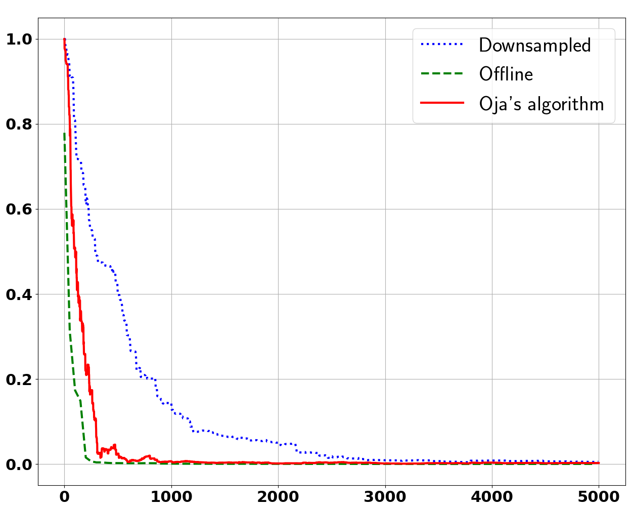
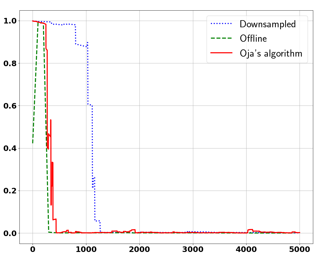
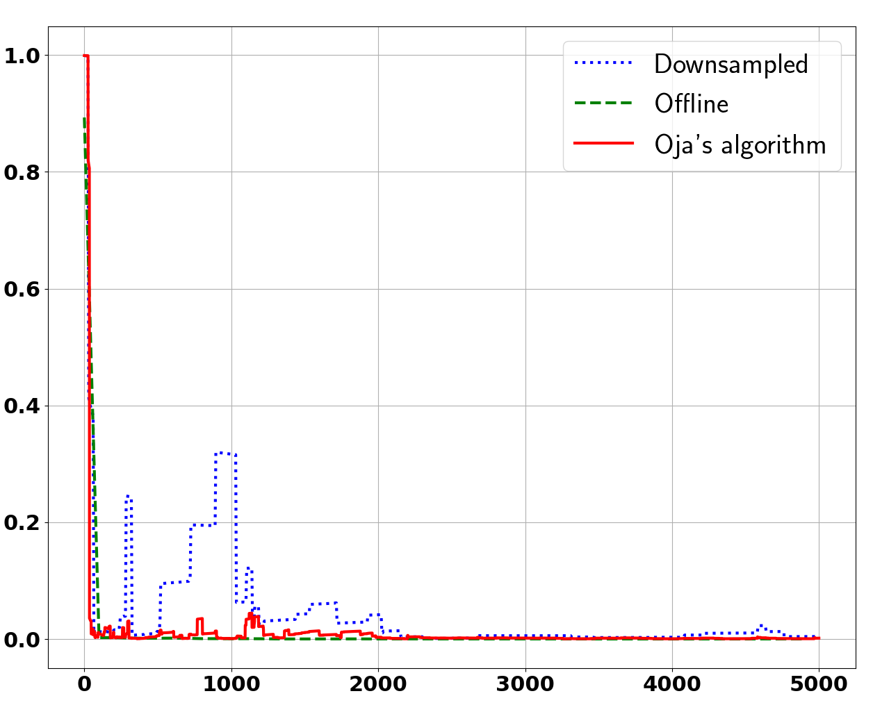
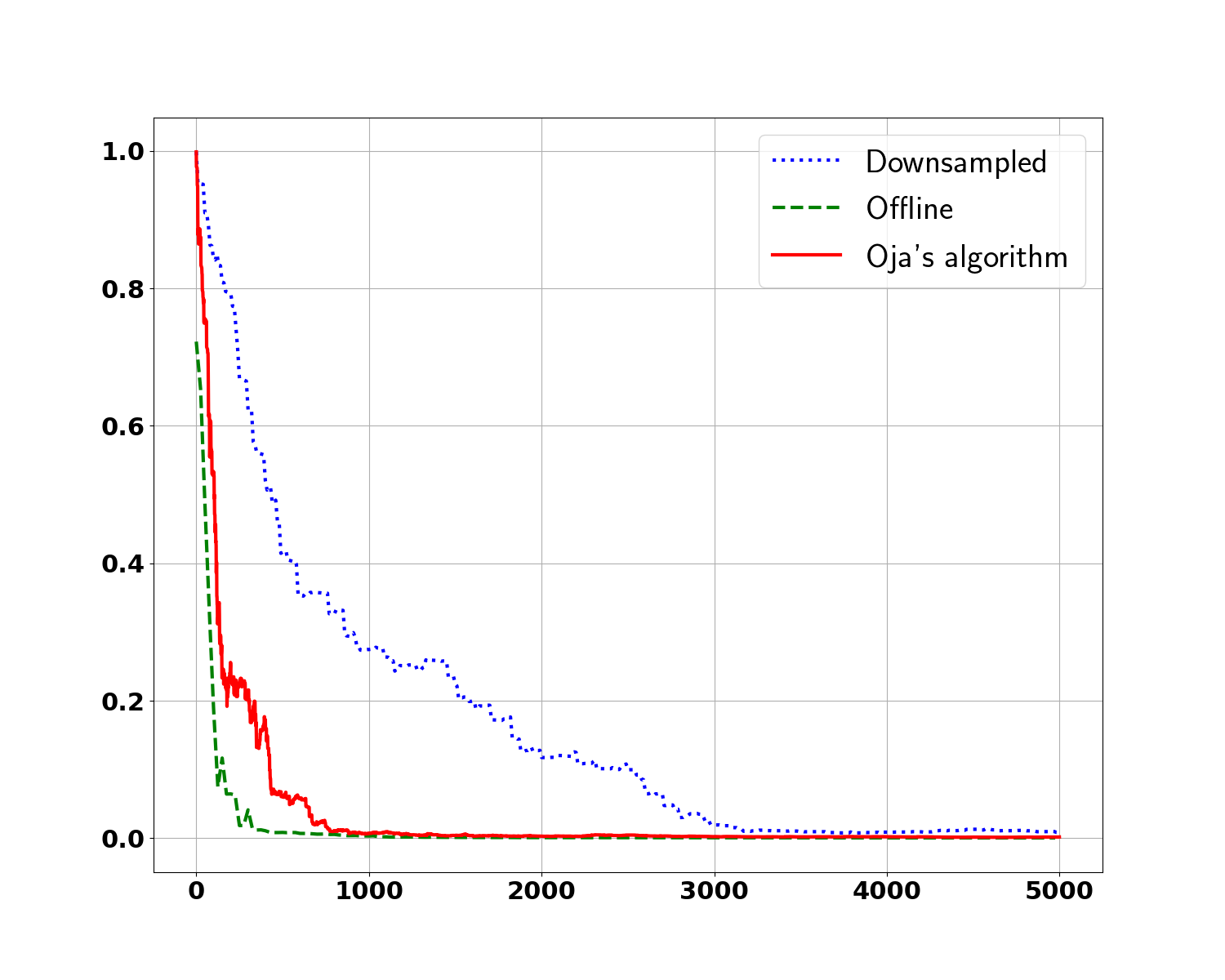
Our contribution: Using a series of approximations, we obtain an optimal error rate for the error, which is worse by a factor of from the corresponding error rate of the IID case. Previous work [3] has established rates worse by a poly-logarithmic factor by using downsampling, i.e. applying the update on every datapoint. In Figure 1, we compare Oja’s algorithm with its downsampled and offline variants (see Section 6 for more details on setup). We see that Oja’s algorithm performs significantly better than the downsampled variant, and similarly to the offline variant where for the data point we compute the eigenvector of the sample covariance matrix of all data-points up-to . Our work provides a concrete and novel result that explains these observations. In Table 1, we compare our bounds with related analyses of Oja’s algorithm. The last row shows that we are the first to obtain an error whose main term is free of logarithmic dependence on or for streaming PCA in the Markovian case.
We break the logarithmic barrier in previous work by considering a series of approximations of finer granularity which uses reversibility of the Markov chain and standard mixing conditions of irreducible and aperiodic Markov chains. Our rates are comparable to the recent work of [27] (Proposition 1) that establishes an offline error analysis for estimating the principal component of the empirical covariance matrix of Markovian data by using a Matrix Bernstein inequality. Our results also imply a linearly convergent decentralized algorithm for streaming PCA in a distributed setting. As a simple byproduct of our theoretical result, we also obtain a rate for Oja’s algorithm applied on downsampled data, which is worse by a factor of , as shown in Figure 1. To our knowledge, this is the first work that analyzes the Markovian streaming PCA problem without any downsampling that matches the error of the offline algorithm.
The crux of our analysis uses the mixing properties of the Markov chain. Strong mixing intuitively says that the conditional distribution of a state in timestep given the starting state is exponentially close to the stationary distribution of , the closeness being measured using the total variation distance. All previous work on Markovian data exploits this property by conditioning on states many time steps before. However, it is crucial to a) adaptively find how far to look back and b) bound the error of the sequence of matrices we ignore between the current state and the state we are conditioning on. Observe that these two components are related. Looking back too far makes the dependence very small but increases the error resulting from approximating a larger matrix product of intermediate matrices. We present a fine analysis that balances these two parts and then uses spectral theory to bound the second part within a factor of a variance parameter that characterizes the variability of the matrices and shows up in the analysis of [15, 27].
| Paper | Markov? | Online? | Log-free | error rate | Sample-Complexity |
| main-term | |||||
| Jain et al. | N | Y | Y | ||
| [15] | N | N | |||
| Chen et al. | Y | Y | N | - | |
| [3] | |||||
| Neeman et al. | Y | N | N | ||
| [27] | |||||
| Theorem 1 | Y | Y | Y |
Related work on streaming PCA and online matrix decomposition on Markovian data: Amongst recent work, [3] is very relevant to our setting, since it analyzes Oja’s algorithm with Markovian Data samples. Inspired by the ideas of [8], the authors propose a downsampled version of Oja’s algorithm to reduce dependence amongst samples and provide a Stochastic Differential Equation (SDE) based analysis to achieve a sample complexity of for error smaller than , where is a variance parameter. We obtain a similar rate in Corollary 1 through our techniques. However, comparing with Theorem 1, we observe that downsampling leads to an extra factor. It is important to point out that [3] provides an analysis for estimating top principal components, whereas this paper focuses on obtaining a sharp rate for the first principal component. [21] consider the harder problem of online non-negative matrix factorization for Markovian data. Their analysis establishes asymptotic convergence of error, but does not provide a rate.
Stochastic Optimization with Markovian Data : Markovian models are often considered in Reinforcement Learning and Linear Dynamic Systems[2, 5, 9, 30, 4, 34, 18, 23]. There have been many notable nonasymptotic bounds for stochastic gradient descent (SGD) methods for general convex and nonconvex functions with Markovian data [8, 31, 6, 7, 10, 38, 33]. The convergence rates (sample complexities) obtained in these works apply to more general problems but do not exploit the matrix product structure inherent to Oja’s algorithm. In this work, we develop novel techniques to show that a sharper analysis is possible for the PCA objective. The paper is organized as follows. Section 2 contains the problem setup and preliminaries about Markov Chains. Section 3 contains Theorem 1. We present a sketch of the main technical tools in Section 4, intermediate theorems needed for the main theorem in Section 5 and conclude with simulations in Section 6.
2 Problem Setup and Preliminaries
This section presents the problem setup and outlines important properties of the Markov chain that will be utilized subsequently. We assume that:
Assumption 1.
The Markov chain is irreducible, aperiodic, reversible, and starts in stationarity, with state distribution 111The last assumption may be eliminated by observing an initial burn-in period of ..
Such a Markov chain can arise in various situations, for e.g., while performing random walks on expander graphs which are used extensively in fields such as computer networks, error-correcting codes, and pseudorandom generators. Each state of the Markov chain is associated with a distribution over -dimensional vectors with mean and covariance matrix .
For a random walk on , we define the sequence of random variables , where conditioned on the state , .We represent the mean as and the covariance matrix as , which, for can be expressed as:
In this work, we assume , which is a common assumption in the IID setting (see [15, 1]). While it may be possible to extend our analysis to the non-zero mean case, it is out of the scope of this paper. Therefore, for
Let the eigenvalues of be denoted as . Let denote the leading eigenvector of and denote the matrix with the remaining eigenvectors as columns. We proceed under the following standard assumptions for , (see for eg. [14]).
Assumption 2.
.
Assumption 3.
with probability 1.
Assumption 3 also implies with probability 1. WLOG, we assume . We use to denote the expectation over state and over the state-specific distributions , unless otherwise specified. Define the matrix product
| (2) |
Unrolling the recursion in 1, the output of Oja’s algorithm at timestep is given as . In this work, denotes the Euclidean norm for vectors and the operator norm for matrices unless otherwise specified. denotes the identity matrix.
2.1 Markov chain mixing times
Now we will discuss some well-known properties of an irreducible, aperiodic, and reversible Markov chain (also see [19]). Let denote the second largest absolute eigenvalue of the Markov chain; let the state-distribution of the Markov chain at timestep with be . For any two probability distributions and , recall that the total variational distance is The distance from at the timestep is defined as . For irreducible and aperiodic Markov chains, by Theorem 4.9 in [19], we have for some . The mixing time of the Markov chain is defined as:
| (3) |
As in [19], we will denote . Then, we have . It is worth mentioning the useful relationship between and , given as These results about mixing time are valid for general irreducible and aperiodic Markov chains. A reversible Markov chain satisfies , . For a reversible, irreducible, and aperiodic Markov chain, the gap , is inversely proportional to [19].
3 Main Results
In this section, we present our main result, a near-optimal convergence rate for Oja’s algorithm on Markovian data. As a corollary, we also establish a rate of convergence for Oja’s algorithm applied on downsampled data, where every data-point is considered. Supplement S.5 contains comprehensive proofs of Theorem 1 and Corollary 1 while the proof of Proposition 1 can be found in Supplement Section S.2.
Theorem 1.
Next, we compare the rate of convergence proposed in Theorem 1 with the offline algorithm having access to the entire dataset using a recent result from [27]. Here, the authors extend the Matrix Bernstein inequality [35, 32], to Markovian random matrices. Their setup is much like ours except that the matrix at any state is fixed, i.e., there is no data distribution as in our setup. However, it is easy to extend their result to our setting by observing that conditioned on the state sequence, the matrices are independent under our model, and we can push in the expectation over the state-specific distributions, , whenever required. Therefore, we have the following result -
Proposition 1 (Theorem 2.2 of [27]+Wedin’s theorem).
Observe that Theorem 1 matches the leading term in Eq 1 except the term. We believe, much like the IID case (also see the remark in [15]), this logarithmic term in [27]’s result is removable for large and a constant probability of success.
Remark 1.
The leading term of Theorem 1 is worse by a factor of . Further, it has an additive lower order term due to the covariance between data-points in the Markovian case.
Corollary 1.
(Downsampled Oja’s algorithm) Fix a . If Oja’s algorithm is applied on the downsampled data-stream with every data-point, where then under the conditions of Theorem 1 with appropriately modified and , the output satisfies
with probability atleast . Here is an absolute constant and .
Remark 2.
Data downsampling to reduce dependence amongst samples has been suggested in recent work [26, 22, 3]. In Corollary 1, we establish that the rate obtained is sub-optimal compared to Theorem 1 by a factor. We prove this by a simple yet elegant observation: the downsampled data stream can be considered to be drawn from a Markov chain with transition kernel since each data-point is steps away from the previous one. For sufficiently large , this implies that the mixing time of this chain is . These new parameters are used to select the modified values of according to Lemma S.12 in the Supplement.
The proof of Theorem 1 follows the same general recipe as in [15] for obtaining a bound on the error. However, the original proof techniques heavily rely on the IID setting. We carry out a refined analysis for each step under the Markovian data model by a careful control of error terms arising out of dependence. The first step involves obtaining a high-probability bound on the error, by noting that Oja’s algorithm on data-points can be viewed as a single iteration of the power method on . Therefore, fixing a using Lemma 3.1 from [15], we have with probability at least ,
| (6) |
where is an absolute constant. The numerator is bounded by first bounding its expectation (see Theorem 3) and then using Markov’s inequality. To bound the denominator, similar to [15], we will use Chebyshev’s inequality. Theorem 4 provides a lower bound for the expectation . Chebyshev’s inequality also requires upper-bounding the variance of , which requires us to bound (see Theorem 5).
4 Main Technical Tools
In this section, we provide a sketch of the main arguments used in our proof.
Warm-up with downsampled Oja’s algorithm: We start with the simple downsampled Oja’s algorithm to build intuition. Here, one applies Oja’s update rule (Eq 1) to every data-point, for a suitably chosen . For , the total variation distance between any consecutive data-points in the downsampled data stream is . As we show in Corollary 1, the error of this algorithm is similar to the error of Oja’s algorithm applied to data-points in the IID setting, i.e., .
We will take as an example. Let us introduce some notation.
| (7) |
We peel this quantity one matrix at a time from the inside. Note that for a reversible Markov chain, standard results imply (see Lemma 1) that the mixing conditions apply to the conditional distribution of a state given another state steps in the “future” (see Supplement section S.3 for a proof). Recall from Section 2.1.
Lemma 1.
Under Assumption 1, .
It will be helpful to explain our analysis by comparing it with the IID setting. For this reason, we will use to denote the expectation under the IID data model.
| (8) |
where the first term is smaller than . We define and as follows. , and .
For the IID setting, the second term is zero, and the third term can be bounded as follows:
Let us denote the IID version of by . The final recursion for the IID case becomes: So, for our Markovian data model, the hope is that the cross term (which has a multiplicative factor of ) is and is . We will start with the term, which is zero in the IID setting.
We hope to reduce the product into a product of nearly independent matrices. One hope is that if instead of , we had for some suitably large integer , then using (reverse) mixing properties of the Markov chain, we could argue using Lemma 1 that is very close to zero.The following lemma formally bounds the deviation of the length- matrix product from identity.
Lemma 2.
Let Assumption 3 hold. If and forms a non-increasing sequence then ,
| (9) | |||
| (10) |
Lemma 2 bounds the norm of the matrix product at two levels. The first result provides a coarse bound, approximating linear and higher-order terms. The second result provides a finer bound, preserving the linear term and approximating quadratic and higher-order terms. The proofs involve a straightforward combinatorial expansion of and are deferred to the Supplement section S.3.
Approximating requires to be small. Since this is a recursive argument, we would need to be small for , which is satisfied by the strong condition is small. To obtain a tight analysis, we choose adaptively. We set (see definition in Eq 3).
As we will show in detail in the Supplement, Lemma 2 Eq 10 along with the adaptive choice of gives us a sharp error bound. Using it, we can bound (see Eq 8) as:
Naively bounding the term by leads to the same rate as downsampled Oja’s algorithm.
In the following lemma, we will establish that, indeed, has a much smaller norm. The novelty of our bound is not just in using the mixing properties of the Markov chain but also in teasing out the variance parameter . We will state the lemma, in a slightly more general form as -
Lemma 3.
Lemma 3 bounds the norm of the covariance between matrices and . In particular, this implies that the norm of decays as . The proof uses a spectral argument that replaces a coarse approximation by a sum of terms to sum of exponentially decaying terms, thereby removing the dependence on , which can be as large as . The proof is deferred to the Supplement section S.4. The details can be found in Supplement section S.4.
Let be positive constants for ease of notation. Coming back to Eq 8, we can bound as follows: . A similar argument can be applied to bound as: . Putting everything together in 8, we have
Recursing on this inequality gives us our bound on (Theorem 2). We are now ready to present all our accompanying theorems.
5 Intermediate Theorems for Convergence Analysis
In this section, we present our accompanying theorems which are used to obtain the main result in Theorem 1. But before doing so, we will need to establish some notation. Let , and the step-sizes be set as with as defined in Theorem 1. Let . As shown in Lemma S.12 in Supplement Section S.3 our choice of step-sizes satisfy, ,
-
C.1
C.2 (Slow decay)
Further, we define scalar variables -
| (11) |
and recall the definitions of and in Eqs 2 and 7, respectively. We are now ready to present the theoretical results needed to prove our main result. For simplicity of notation, we present versions of the results by using with as defined in Theorem 1. However, these theorems are in fact valid under more general step-size schedules. We state and prove the more general versions in the Supplement Section S.4.
The three primary differences with the IID case are a) the term, which arises since the recursion sketched in Section 4 leaves out the last terms which are bounded by ; (b) the new factor of with due to the Markovian dependence between terms; and c) the extra lower order term arising from the use of Lemmas 2 and 3.
Here, the difference is mainly in the new variable , arising since the recursion stops at , not . represents the approximation of the first terms.
This differs from its IID counterpart by a multiplicative factor of for the same reason as before, which also makes the sums go up to instead of . Note that for sufficiently large (Lemma S.13), is very small and . Therefore, as large .
The differences are similar to the last theorems involving . Surprisingly, for this, the coarse approximation suffices, leading to an absence of the term in the bound. Having established these results, the final step is to substitute them into Eq 6 and follow the proof recipe described earlier. This requires significant calculations and is deferred to the Supplement Section S.5.
6 Experimental Validation
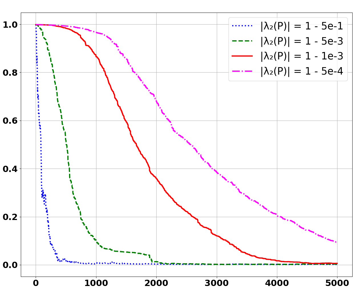
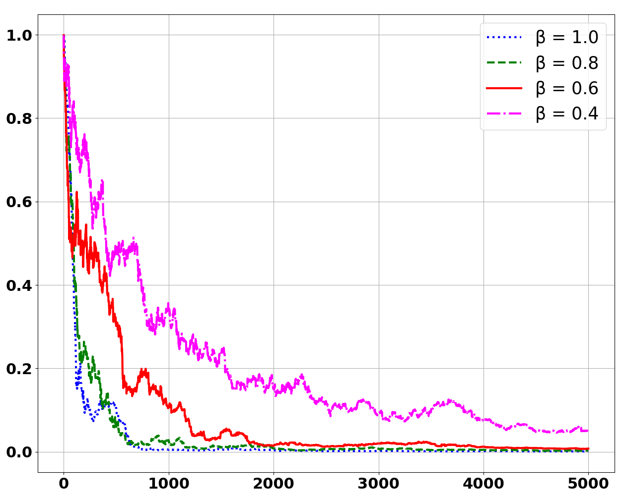
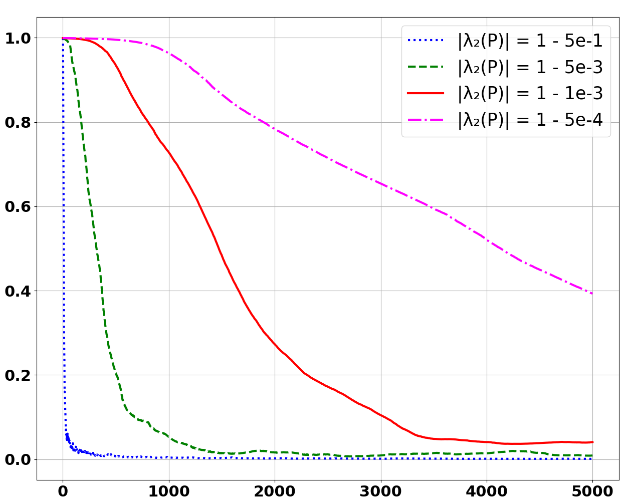
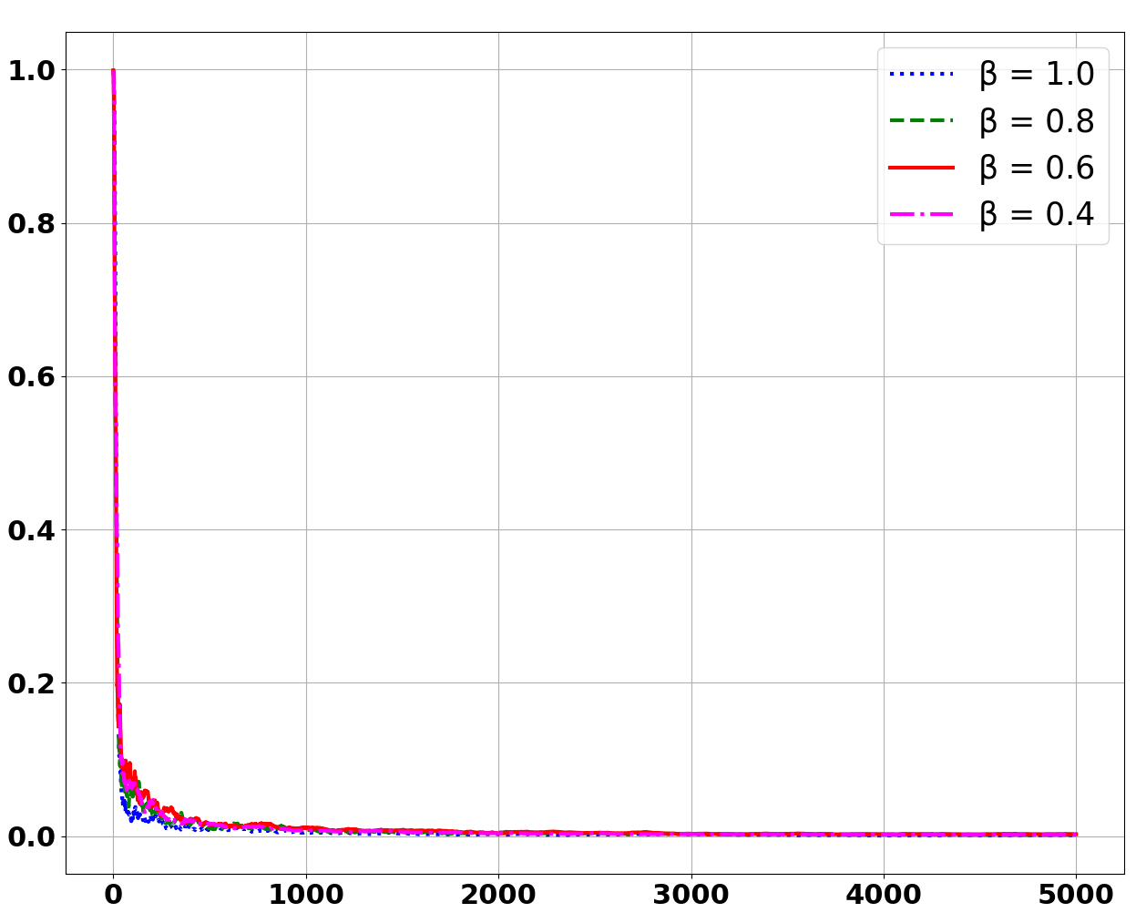
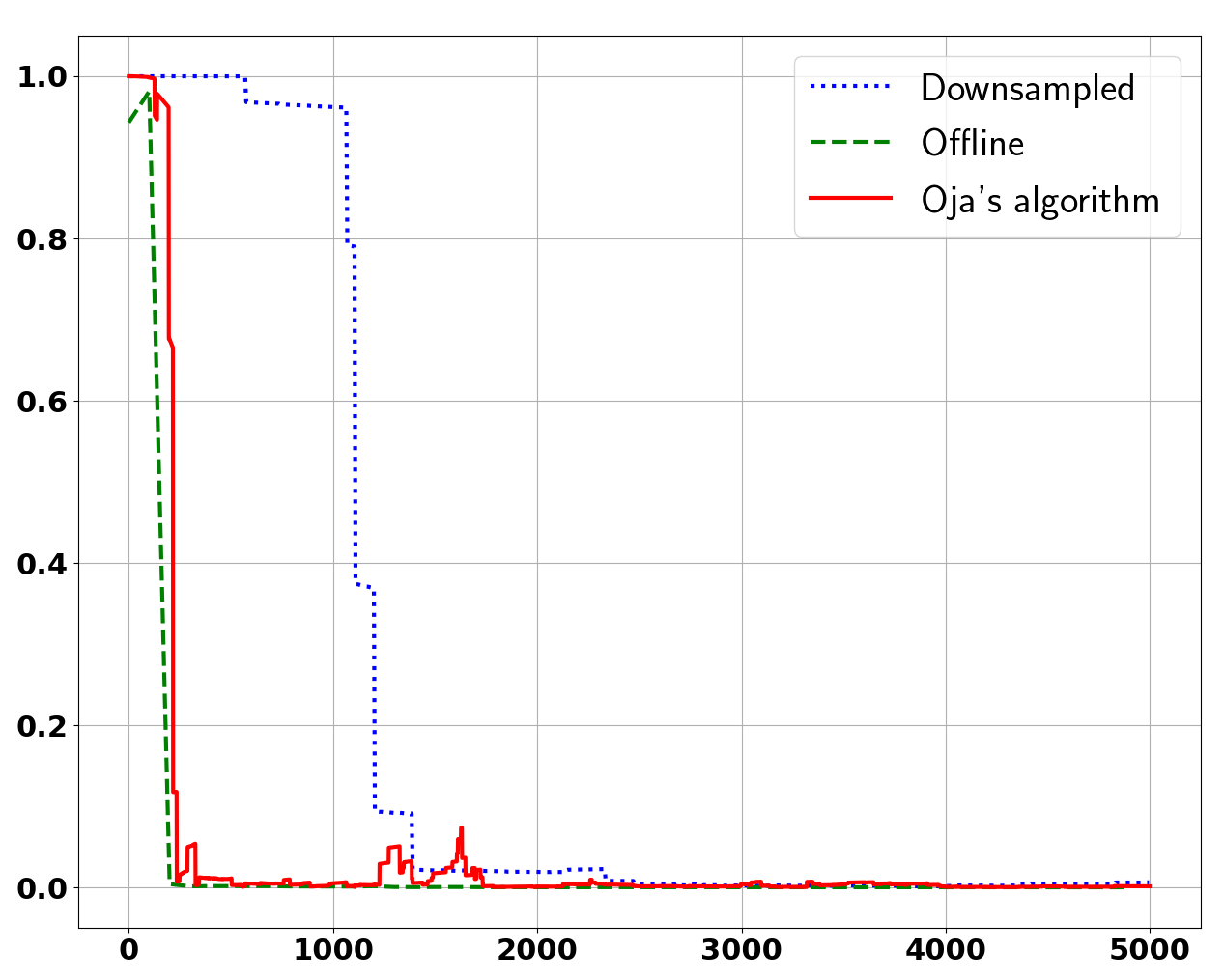
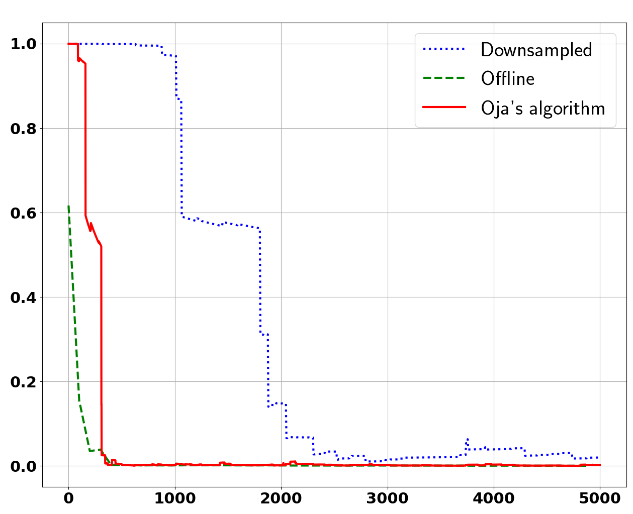
In this section, we present some simple experiments to validate our theoretical results. For more detailed experiments, see the Supplement. We design a Markov chain with states, where the transition matrix entries equal for and for . Smaller values of lead to larger mixing times. It can be verified that the stationary distribution is uniform over the state-space and . We set for Figures 1 and 2(a), and vary it in Figure 2(b). Each point in the plot is averaged over 20 random runs over different Markov chains, datasets, and initialization.
Each state is associated with Bernoulli() distribution. We set and select at the start of each random run. The covariance matrix, , for each state is set as where . We start with the stationary distribution , and for each state , we draw IID samples . We standardize such that all components have zero mean and unit variance under the state distribution, . We then generate the sample data-point for PCA as . By construction, and . The step sizes for Oja’s algorithm are set as for . For the downsampled variant, every data-point is considered, and is accordingly divided by 10. For the offline algorithm, we recompute the leading eigenvector of the sample covariance matrix of data-points seen so far.
Figure 1 compares the performance of different algorithms for the Bernoulli distribution. Here, we are checking if the results obtained in Theorem 1, Proposition 1, and Corollary 1 are reflected in the experiments.
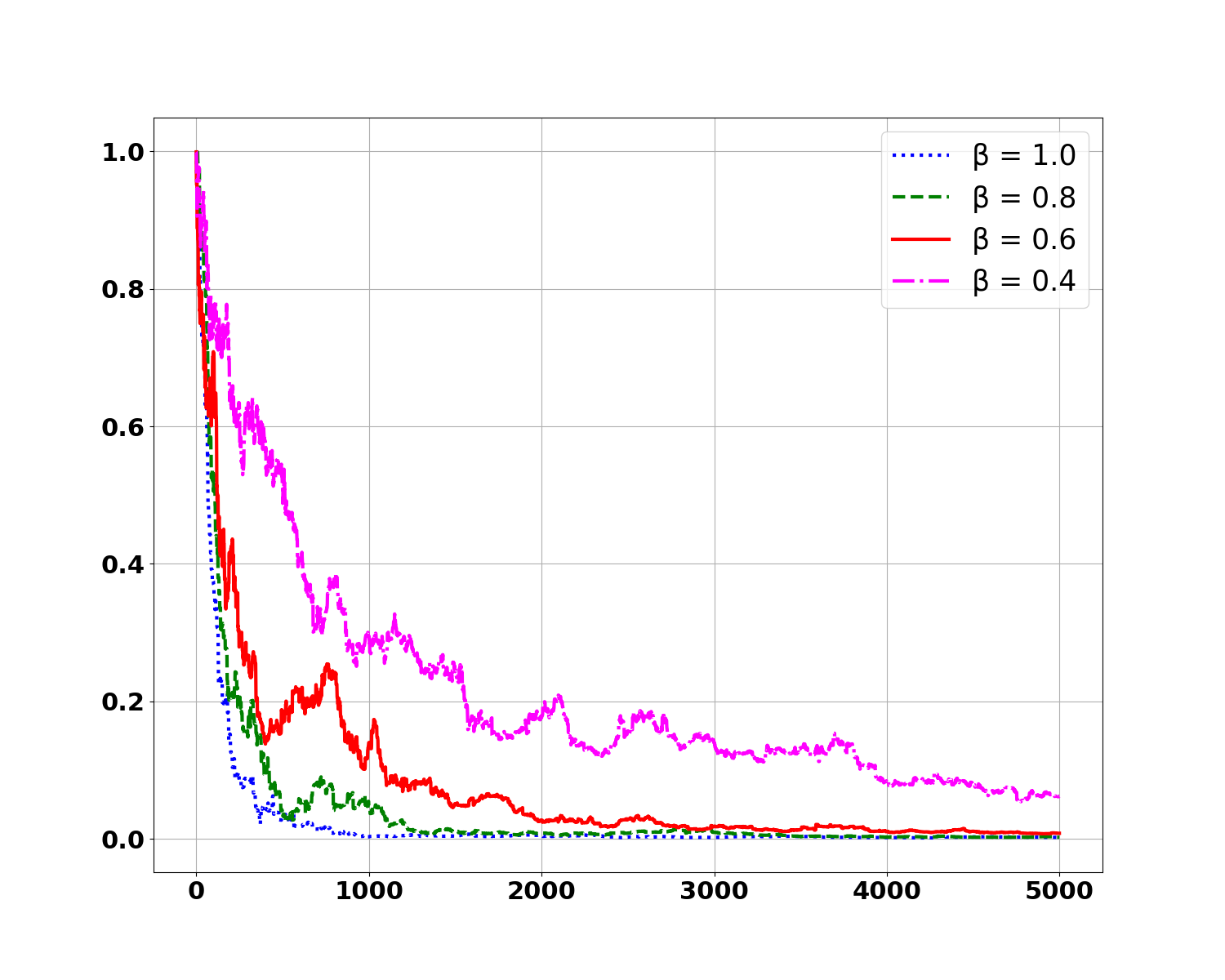
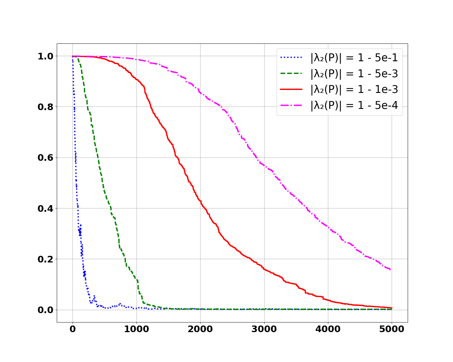
The experimental results demonstrate that Oja’s algorithm performs significantly better than the downsampled version, consistent with the theoretical results. It also shows that Oja’s algorithm performs similarly to the offline algorithm, which is also confirmed by our theoretical results and that of [27]. Figure 2(a) compares the performance of Oja’s algorithm for different covariance matrices. Smaller values of decrease the eigengap , and hence lead to a slower convergence. Figure 2(b) confirms that smaller values of (larger values of ) also worsen the rate, which matches with our theoretical results.
7 Conclusion
We have considered the problem of streaming PCA for Markovian data, which has implications in various settings like decentralized optimization, reinforcement learning, etc. The analysis of streaming algorithms in such settings has seen a renewed surge of interest in recent years. However, the dependence between data-points makes it difficult to obtain sharp bounds. We provide, to our knowledge, the first sharp bound for obtaining the first principal component from a Markovian data stream that breaks the logarithmic barrier present in the analysis done for downsampled data. We believe that the theoretical tools that we have developed in this paper would enable one to obtain sharp bounds for other dependent data settings, learning top principal components, and online inference algorithms with updates involving products of matrices.
8 Acknowledgements
We gratefully acknowledge NSF grants 2217069 and DMS 2109155. We are also grateful to Rachel Ward and Bobby Shi for valuable discussions.
References
- [1] Zeyuan Allen-Zhu and Yuanzhi Li. First efficient convergence for streaming k-pca: a global, gap-free, and near-optimal rate. In 2017 IEEE 58th Annual Symposium on Foundations of Computer Science (FOCS), pages 487–492. IEEE, 2017.
- [2] Jalaj Bhandari, Daniel Russo, and Raghav Singal. A finite time analysis of temporal difference learning with linear function approximation. CoRR, abs/1806.02450, 2018.
- [3] Minshuo Chen, Lin Yang, Mengdi Wang, and Tuo Zhao. Dimensionality reduction for stationary time series via stochastic nonconvex optimization. Advances in Neural Information Processing Systems, 31, 2018.
- [4] Shuhang Chen, Adithya Devraj, Ana Busic, and Sean Meyn. Explicit mean-square error bounds for monte-carlo and linear stochastic approximation. In International Conference on Artificial Intelligence and Statistics, pages 4173–4183. PMLR, 2020.
- [5] Thinh T. Doan, Lam M. Nguyen, Nhan H. Pham, and Justin Romberg. Convergence rates of accelerated markov gradient descent with applications in reinforcement learning, 2020.
- [6] Thinh T. Doan, Lam M. Nguyen, Nhan H. Pham, and Justin Romberg. Finite-time analysis of stochastic gradient descent under markov randomness, 2020.
- [7] Ron Dorfman and Kfir Yehuda Levy. Adapting to mixing time in stochastic optimization with markovian data. In International Conference on Machine Learning, pages 5429–5446. PMLR, 2022.
- [8] John C. Duchi, Alekh Agarwal, Mikael Johansson, and Michael I. Jordan. Ergodic mirror descent. SIAM J. Optim., 22(4):1549–1578, 2012.
- [9] Alain Durmus, Eric Moulines, Alexey Naumov, Sergey Samsonov, and Hoi-To Wai. On the stability of random matrix product with markovian noise: Application to linear stochastic approximation and td learning. In Conference on Learning Theory, pages 1711–1752. PMLR, 2021.
- [10] Mathieu Even. Stochastic gradient descent under markovian sampling schemes, 2023.
- [11] Andreas Grammenos, Rodrigo Mendoza-Smith, Cecilia Mascolo, and Jon Crowcroft. Federated PCA with adaptive rank estimation. CoRR, abs/1907.08059, 2019.
- [12] Anne Hartebrodt, Reza Nasirigerdeh, David B. Blumenthal, and Richard Röttger. Federated principal component analysis for genome-wide association studies. In 2021 IEEE International Conference on Data Mining (ICDM), pages 1090–1095, 2021.
- [13] Amelia Henriksen and Rachel Ward. AdaOja: Adaptive Learning Rates for Streaming PCA. arXiv e-prints, page arXiv:1905.12115, May 2019.
- [14] De Huang, Jonathan Niles-Weed, and Rachel Ward. Streaming k-pca: Efficient guarantees for oja’s algorithm, beyond rank-one updates. CoRR, abs/2102.03646, 2021.
- [15] Prateek Jain, Chi Jin, Sham Kakade, Praneeth Netrapalli, and Aaron Sidford. Streaming pca: Matching matrix bernstein and near-optimal finite sample guarantees for oja’s algorithm. In Proceedings of The 29th Conference on Learning Theory (COLT), June 2016.
- [16] Chi Jin, Sham M Kakade, Cameron Musco, Praneeth Netrapalli, and Aaron Sidford. Robust shift-and-invert preconditioning: Faster and more sample efficient algorithms for eigenvector computation. arXiv preprint arXiv:1510.08896, 2015.
- [17] László Kozma. Inequalities cheat sheet, 2018. PDF file.
- [18] Harold J Kushner and G George Yin. Applications in signal processing, communications, and adaptive control. Stochastic Approximation and Recursive Algorithms and Applications, pages 63–93, 2003.
- [19] David A Levin and Yuval Peres. Markov chains and mixing times, volume 107. American Mathematical Soc., 2017.
- [20] Robert Lunde, Purnamrita Sarkar, and Rachel Ward. Bootstrapping the error of oja’s algorithm. Advances in Neural Information Processing Systems, 34:6240–6252, 2021.
- [21] Hanbaek Lyu, Deanna Needell, and Laura Balzano. Online matrix factorization for Markovian data and applications to Network Dictionary Learning. arXiv e-prints, page arXiv:1911.01931, November 2019.
- [22] Shaocong Ma, Ziyi Chen, Yi Zhou, Kaiyi Ji, and Yingbin Liang. Data sampling affects the complexity of online sgd over dependent data. In Uncertainty in Artificial Intelligence, pages 1296–1305. PMLR, 2022.
- [23] Abdelkader Mokkadem. Mixing properties of arma processes. Stochastic Processes and their Applications, 29(2):309–315, 1988.
- [24] Jean-Marie Monnez. Stochastic approximation of eigenvectors and eigenvalues of the q-symmetric expectation of a random matrix. Communications in Statistics-Theory and Methods, pages 1–15, 2022.
- [25] Nikos Mouzakis and Eric Price. Spectral guarantees for adversarial streaming pca, 2022.
- [26] Dheeraj Nagaraj, Xian Wu, Guy Bresler, Prateek Jain, and Praneeth Netrapalli. Least squares regression with markovian data: Fundamental limits and algorithms. Advances in neural information processing systems, 33:16666–16676, 2020.
- [27] Joe Neeman, Bobby Shi, and Rachel Ward. Concentration inequalities for sums of markov dependent random matrices, 2023.
- [28] Erkki Oja. Simplified neuron model as a principal component analyzer. Journal of Mathematical Biology, 15(3):267–273, November 1982.
- [29] Erkki Oja and Juha Karhunen. On stochastic approximation of the eigenvectors and eigenvalues of the expectation of a random matrix. Journal of mathematical analysis and applications, 106(1):69–84, 1985.
- [30] Rayadurgam Srikant and Lei Ying. Finite-time error bounds for linear stochastic approximation andtd learning. In Conference on Learning Theory, pages 2803–2830. PMLR, 2019.
- [31] Tao Sun, Yuejiao Sun, and Wotao Yin. On markov chain gradient descent. Advances in neural information processing systems, 31, 2018.
- [32] Joel A Tropp. User-friendly tail bounds for sums of random matrices. Foundations of computational mathematics, 12:389–434, 2012.
- [33] Lan V Truong. Generalization error bounds on deep learning with markov datasets. Advances in Neural Information Processing Systems, 35:23452–23462, 2022.
- [34] John Tsitsiklis and Benjamin Van Roy. Analysis of temporal-diffference learning with function approximation. In M.C. Mozer, M. Jordan, and T. Petsche, editors, Advances in Neural Information Processing Systems, volume 9. MIT Press, 1996.
- [35] Roman Vershynin. Introduction to the non-asymptotic analysis of random matrices. arXiv preprint arXiv:1011.3027, 2010.
- [36] Per-Åke Wedin. Perturbation bounds in connection with singular value decomposition. BIT Numerical Mathematics, 12:99–111, 1972.
- [37] Puyudi Yang, Cho-Jui Hsieh, and Jane-Ling Wang. History pca: A new algorithm for streaming pca. arXiv preprint arXiv:1802.05447, 2018.
- [38] Ingvar Ziemann and Stephen Tu. Learning with little mixing. In S. Koyejo, S. Mohamed, A. Agarwal, D. Belgrave, K. Cho, and A. Oh, editors, Advances in Neural Information Processing Systems, volume 35, pages 4626–4637. Curran Associates, Inc., 2022.
Supplement
The Supplement is organized as follows -
Appendix S.1 Notation and assumptions
For conciseness, we define the stochastic function which maps each state variable of the Markov chain to a () positive semi-definite symmetric matrix as
Where is drawn from the distribution corresponding to the state at timestep . All the theoretical results are derived under Assumptions 1, 2 and 3.
Appendix S.2 Offline PCA with Markovian Data
In this section, we prove Proposition 1. We note that [27] considers to be random only with respect to the states. Therefore, we first show that their results generalize to our setting as well, using . From Eq in [27], we have
where . Noting that conditioned on the state sequence, the matrices are independent under our model, we can push in the expectation over the state-specific distributions inside. Let denote the expectation over the stationary state-sequence of the Markov chain, and denote the distribution over states. Therefore,
Defining the multiplication operator for any vector-valued function , we note that Eq from [27] holds for our case as well.
Next, we adapt Proposition 5.3 from [27] for our setting. Specifically, we have the following lemma -
Lemma S.1.
Proof.
Finally, to prove Bernstein’s inequality, we prove that Lemma 6.7 from [27] holds for our case. To note this, we start with equation (57) in their work. We have, using Lemma S.1,
Therefore, Eq from [27] follows. The other bounds in the proof of Lemma 6.7 from [27] follow similarly. Therefore, we have the following version of Theorem 2.2 from [27] -
Appendix S.3 Useful Results
This section presents some useful lemmas and their proofs that are subsequently used in our proofs.
Lemma S.2.
(Reverse mixing) Consider a reversible, irreducible, and aperiodic Markov chain started from the stationary distribution. Then,
Proof.
Let the transition probabilities of the Markov chain be represented as . Consider the time-reversed chain for . Then,
This proves that is an irreducible Markov chain with the same transition probabilities as the original Markov chain. The irreducibility of follows from the original Markov chain being irreducible. Therefore,
| (S.12) |
Then,
where the last inequality follows from the forward mixing properties of the Markov chain. ∎
Lemma S.3.
Let for , where are symmetric PSD matrices. Let . Then,
Proof.
Since and are both PSD, the second term on the RHS is always positive. This yields the proof. ∎
Lemma S.4.
Let , where are symmetric PSD matrices.
Proof.
Since and are both PSD, the last two terms on the RHS are always positive. This yields the proof. ∎
Lemma S.5.
Consider matrices and . Then,
Proof.
For a matrix , let the singular values be denoted as :
Using Von-Neumann’s trace inequality, we have
∎
Lemma S.6.
Given the Markov property in a Markov chain, the reverse Markov property holds, i.e
Proof.
∎
S.3.1 Proof of Lemma 2
Now we are ready to provide a proof of Lemma 2.
Proof of Lemma 2.
Without loss of generality, we prove the statement for . For convenience of notation, we denote . Note that,
with the convention that . Therefore, since forms a non-increasing sequence and , we have,
| (S.13) |
where we have used the assumptions that , and the useful result that
| (S.14) |
This completes the proof for .
For part , we have
| (S.15) |
which completes the proof. ∎
S.3.2 Proof of Lemma 3
Before proving Lemma 3, we will need the following lemma.
Lemma S.7.
For arbitrary matrices and , we have
where denotes the spectral norm.
Proof.
Define matrix as . We note that
Then, we have,
which completes our proof. ∎
Proof of Lemma 3.
We denote for convenience of notation. By using reversibility (see S.12), we know that the time-reversed process is also a Markov chain with the same transition probabilities. Then, for and any ,
| (S.16) |
Step (i) uses reversibility. Therefore,
| using Lemma S.6 | |||
| using Eq S.3.2 | |||
Therefore, without loss of generality, we proceed with the second form.
| (S.17) |
| (S.18) |
For , we have,
| (S.19) |
For , we have,
| (S.20) |
Step uses Lemma S.7 with and . Let’s now bound . Let and . Then, we have
Now, since we have a reversible Markov chain, . Therefore,
Therefore, is similar to the self-adjoint matrix and their eigenvalues are real and the same. Further note that is the leading eigenvector of with eigenvalue 1 since
Now,
where denotes the second-largest eigenvalue in magnitude. Therefore, using S.17, S.19 and S.20, we have
Hence proved. ∎
Lemma S.8.
Let and forms a non-increasing sequence. Set . Then for constant matrix , and constant positive semi-definite matrix , , we have
where is defined in 7.
Proof.
For the convenience of notation, we denote . Let , then
| (S.21) |
We will now bound each of the terms and .
Now, using Lemma 1, we have,
| (S.22) |
where we have used Lemma S.5. Therefore,
| (S.23) |
We will now bound . Let . Using Lemma 2 we have
Then,
Using Lemma 3 with we have,
| (S.24) |
Therefore,
| (S.25) |
Similarly using Lemma 3 with ,
| (S.26) |
Finally,
| (S.27) |
Therefore, using Eqs S.23, S.25, S.26, S.27 along with S.21, we have
where in the last line we used . Hence proved. ∎
Lemma S.9.
Let and forms a non-increasing sequence. Set . Then for constant matrices , , , we have
where is defined in 7.
Proof.
For convenience of notation, we denote . Let , then
We will now bound each of the terms and .
Since , therefore
where in , we used similar steps as S.22 to get
| (S.28) |
Next, using Lemma 2 we have that
| (S.29) |
Therefore,
Similarly,
Finally, using the bound on from Eq S.29, we have:
Therefore,
where in , we used . Hence proved. ∎
Lemma S.10.
Let and step-sizes forms a non-increasing sequence. Further, let the step-sizes follow a slow-decay property, i.e, . Set . Let be a constant positive semi-definite matrix, and , then,
where is defined in 2.
Proof.
Let with . Then,
Let’s consider each of the terms above. Using Von-Neumann’s trace inequality and S.25, we have,
Therefore we have,
where in we used along with in . Hence proved. ∎
Lemma S.11.
Let and forms a non-increasing sequence. Set . Let be a constant matrix and . Further, let the decay of the step-sizes be slow such that . Then
where is defined in 2.
Proof.
Let with . Then,
Let’s consider each of the terms above. Using Von-Neumann’s trace inequality and noting that , we have
Therefore, we have
In , we used the slow-decay assumption on mentioned in the lemma statement along with . Hence proved. ∎
Lemma S.12.
(Learning Rate Schedule) Fix any . Set . Suppose the step sizes are set such that
Define the linear function
With and defined in S.4, set and
then we have
-
1.
-
2.
(slow-decay)
-
3.
-
4.
Proof.
We use the following inequalities -
| (S.30) | |||
| (S.31) | |||
| (S.32) | |||
| (S.33) |
For the first result, we observe that is a decreasing function of for . Using properties of the mixing time (see Section 2.1 in the manuscript), we have
| (S.34) |
for . For
Therefore,
From the assumptions mentioned in the Lemma statement, we have
| (S.35) |
Therefore,
| (S.36) |
For the second result, we note that ,
Consider the fraction . We can simplify it as :
where we used the fact that is an increasing function for . Therefore, we have that
For the third result, we note that
Therefore,
| (S.37) |
where follows from the slow decay property of .
For , using S.30 we have,
| (S.38) |
For , substituting the value of from S.34 for we have,
| (S.39) | ||||
| (S.40) |
Note that is a linear function of and . We observe that is a decreasing function of for . Therefore,
Substituting in S.40 we have,
Putting everything together in S.37 and using the bounds on mentioned in the lemma statement, we have,
Finally, for the last result we first note that
Therefore,
| (S.41) |
Let’s define
Note that since ,
Then,
| (S.42) |
Using S.31, . Noting that , we have
| (S.43) |
and similarly,
| (S.44) |
Using S.36, we have
| (S.45) |
Therefore, using [17]
| (S.46) |
where follows since by S.45 and follows since .
Appendix S.4 Proofs : Convergence Analysis of Oja’s Algorithm for Markovian Data
In this section, we present proofs of Theorems 2, 3, 4 and 5. We state versions of these theorems that are valid under more general conditions on the step sizes. Specifically, for the following, we only require a sequence of non-increasing step-sizes which satisfy, for -
-
C.1
C.2 (Slow decay)
The version of these theorems stated in the main manuscript are obtained by plugging in the step-sizes as for the values of provided in Lemma S.12. Before starting with the proofs, we define the following scalar variables -
| (S.49) |
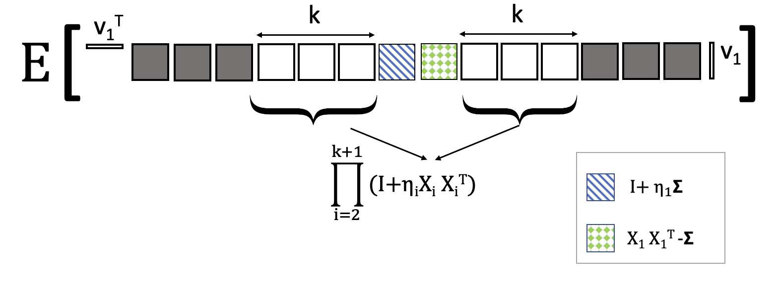
The basic idea behind these proofs is illustrated in Figure S.1, where we are trying to approximate the matrix product by conditioning back in time just the right amount, to balance the tradeoff between the advantage of the mixing decay and the norm of the product of matrices.
Theorem 2.
Proof.
Define . Then, we have
| (S.50) | ||||
Using Lemma S.8 with and noting that , along with observing that from Lemma S.3, we have
We note that , therefore, using the assumption in S.4, .
Next, using Lemma S.9 with and noting that along with observing that using Lemma S.3, we have
where in the last line, we used .
Then from S.50 for ,
| (S.51) |
where is defined as
where in we used .
Then recalling the definition of in S.4, and noting that using Lemma S.3 we have from S.51,
Therefore using this recursion, we have,
Let , where a.s.
Using Lemma 2 we have
Therefore,
Hence proved. ∎
Theorem 3.
Proof.
For , let
Note that by definition. Then,
Let with . Using Lemma S.10 with , where is a diagonal matrix of eigenvalues of , and noting that ,
where in the last line, we used .
Using Lemma S.11 with ,
where in we used and in we used . Putting everything together, we have,
where is as defined in S.4. Therefore using Lemma S.4,
| (S.52) |
Let . From Theorem 2 denoting
| (S.53) |
we have,
Now, we note the definition of and as mentioned in S.4 -
Therefore using S.52,
Recursing on the above inequality for where , we have,
Now, since , therefore, we have
Recall that as defined in S.4. Therefore,
Theorem 4.
Proof.
We will start will expanding the quantity of interest using Eq S.50.
| (S.54) |
where has been defined in Theorem 2. Let’s define
Note that . First we bound . Let . By Lemma 2 along with the slow-decay assumption on the step-sizes, we know that a.s. Then,
Therefore,
| (S.55) |
Now using S.54, we have
First, observe that , where denotes a matrix of eigenvectors of , and is a PSD diagonal matrix. Since for some other PSD diagonal matrix , the product will also be PSD.
By using Lemma S.8 with and noting that , we have
where . Therefore,
Let
as defined in S.4. Unwinding the recursion for , we have,
where second step followed from Theorem 2 and S.55.
Using the inequalities and , we have,
Therefore denoting , we have
where is defined in S.4. Hence proved. ∎
Theorem 5.
Proof.
Define , and . Using S.50, we have, for ,
Thus, we have -
| (S.56) |
Note that,
Now we work on the cross-term. For the convenience of notation, let’s denote unless otherwise specified. Let with,
Using Lemma 2, we have
| (S.57) |
We will also bound
| (S.58) |
So, now we have:
Lets start with the last term, . Using Lemma S.3 we have,
Using Eqs S.4 and S.4 the first three terms can be bounded as:
and similarly,
Note that
Define
Putting everything together in Eq S.56, for we have,
Recall our definition of . We can use the above recursion for . We note that satisfies the conditions. Therefore,
Let , with a.s.
Using Lemma 2, we have
which completes our proof. ∎
Appendix S.5 Main Results : Details and Proofs
S.5.1 Proof of Theorem 1
Lemma S.13.
Proof.
For (1), using Lemma S.12-(3), we note that
| (S.59) | ||||
Therefore,
| (S.60) |
Setting , we have,
which holds for .
For , using Lemma S.12 and substituting the value of for , we note that
Therefore (2) holds for sufficiently large , i.e,
This is satisfied if
| (S.61) |
From Lemma S.12, we have
where follows since and . Therefore, suffices. Further, we note that (2) implies (1) for m = 200, . Therefore, the condition on is sufficient for both results. Hence proved. ∎
Lemma S.14.
Proof.
S.5.1.1 Numerator
Using Theorem 3 and Markov’s Inequality, we have with probability atleast
S.5.1.2 Denominator
Using Chebyshev’s Inequality we have, with probability atleast
| (S.62) |
Let . Using Theorem 3, we have
Using Theorem 4, we have
Let
Then,
By Lemma S.13, we have that
| (S.63) |
Then, using
we have,
By Lemma S.12-(3), we have that
| (S.64) |
By S.59, we have that
| (S.65) |
By Lemma S.13, we have that
| (S.66) |
Then,
Then setting , from S.62 we have
S.5.1.3 Fraction
S.5.2 Proof of Corollary 1
Proof of Corollary 1.
We note that the downsampled data stream can be considered to be drawn from a Markov chain with transition kernel since each data-point is steps away from the previous one. We will denote the parameters of this transformed chain by when the corresponding parameter is under the original chain. For example, is the mixing time of the new chain.
Note that this modified transition matrix has the same stationary distribution . It is also reversible. This can be seen by considering the diagonal matrix of stationary distribution probabilities , where . For a reversible Markov Chain, we have . However, that also implies . This same technique works for yielding .
Using standard results on Markov chains [19],
| (S.69) |
where . Therefore, as noted in the theorem statement, we substitute the modified parameters in the bound we have proven for Theorem 1.
First, we will show that the mixing time for this new chain is . We will use . So by definition the using the definition of in Section 2.1. Hence using conditions on the learning rate schedule imposed in Theorem 1. Therefore, in the transformed chain, the “new” is .
We also have:
We see that . Next, we note that for the transition kernel , the second-largest absolute eigenvalue is given as . Consider the function for . Then,
Therefore, . which implies . Here follows if , which is true. Therefore,
This also implies that the mixing time for the new Markov chain for sub-sampled data is . The bound then follows by substituting to be and setting the in the original expression of Theorem 1 to a constant. ∎
Appendix S.6 Additional Experiments
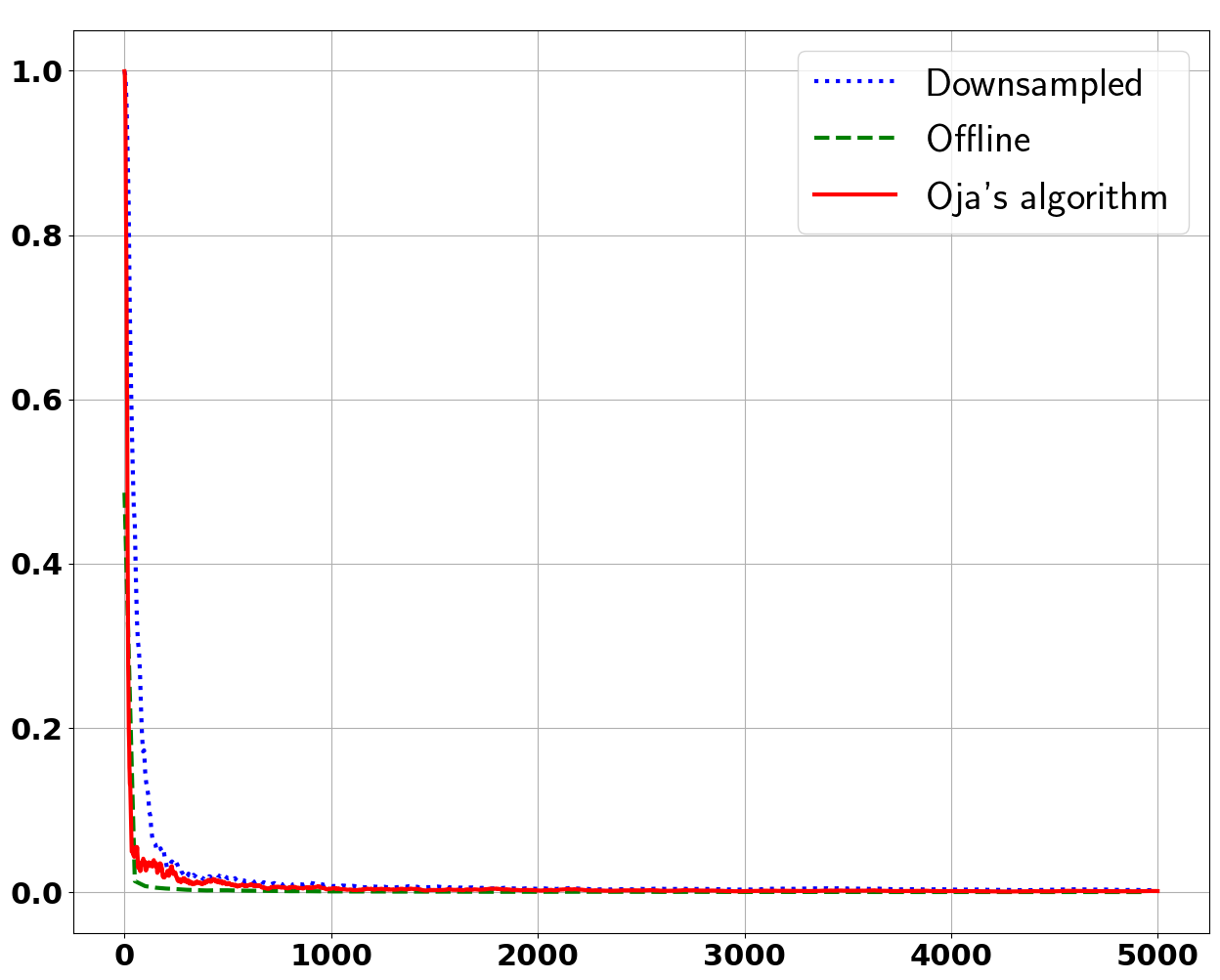
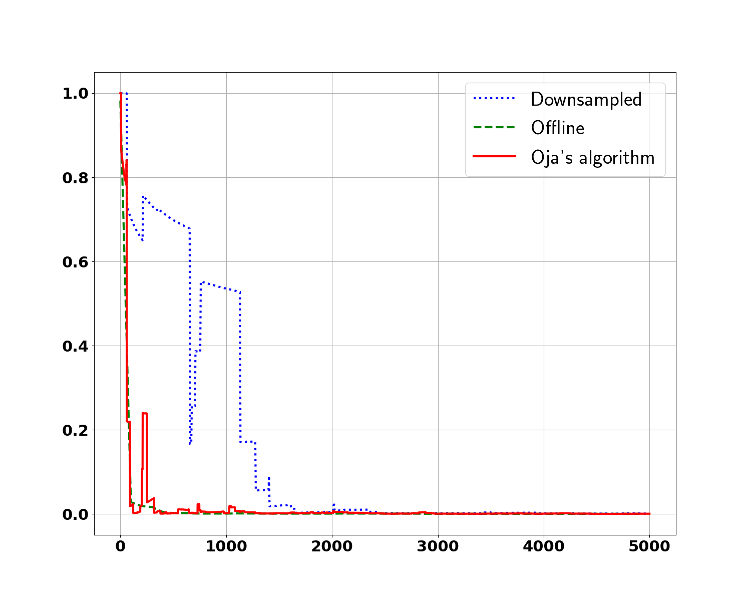
In this section, we provide additional experiments to support the results established in Section 3 of the manuscript. We present experiments with distributions that have nonzero mean vectors at each state, but zero mean with respect to the stationary distribution. This means that the ’s are not necessarily zero-mean with respect to each state distribution . To normalize the data-points, we estimate the mean and covariance matrix empirically from a much larger independently generated dataset.
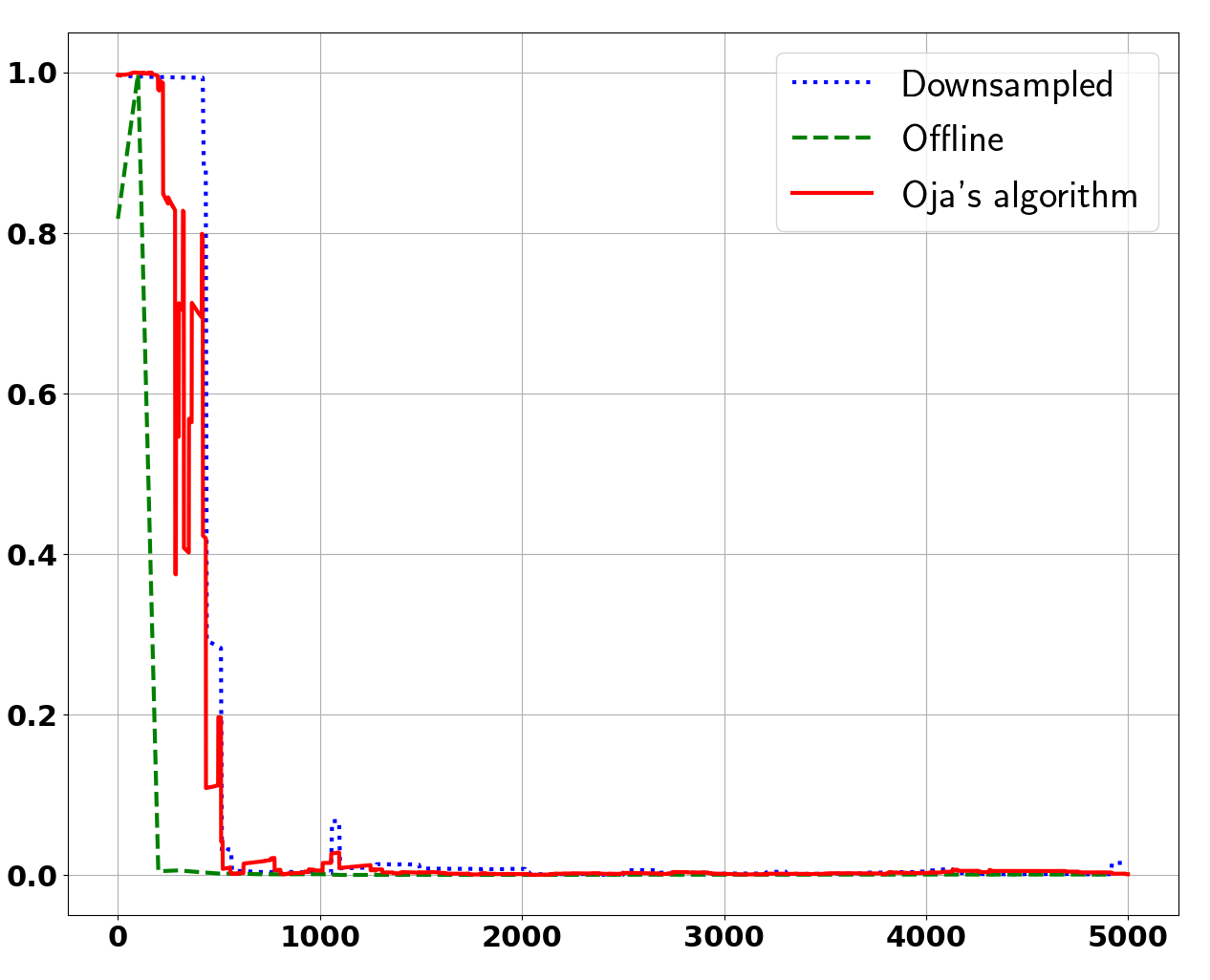
We experiment with two different settings here - Figure S.2 contains the results for each state distribution being Bernoulli() with being fixed for each dataset. Figure S.3 provides results for each state distribution being with being selected at the start of each random run. We observe that these experiments depict similar trends to those shown in the main manuscript, which validates our results for the case of non-zero state means. Furthermore, the Bernoulli data, being sparse compared to the Uniform one, seems to exhibit a clearer difference between data downsampling and the traditional Oja’s algorithm. To provide clear plots demonstrating the relative behavior of the algorithms considered in this paper, we have shown the averaged errors in Figures S.2 and S.3. In Figure S.4 we show six random runs where we fixed the for each state for all runs. These figures clearly show that in general, Downsampled Oja has a worse performance than Oja’s algorithm, which has a similar performance as the offline algorithm. It also shows that the Downsampled algorithm has the most variability, whereas Oja’s algorithm on the whole dataset has much less variability, and finally, and not surprisingly, the offline algorithm has the least variability. Similar qualitative trends can be observed for the other settings.
