Calibrated Explanations:
with Uncertainty Information and Counterfactuals

Abstract

While local explanations for AI models can offer insights into individual predictions, such as feature importance, they are plagued by issues like instability. The unreliability of feature weights, often skewed due to poorly calibrated ML models, deepens these challenges. Moreover, the critical aspect of feature importance uncertainty remains mostly unaddressed in Explainable AI (XAI). The novel feature importance explanation method presented in this paper, called Calibrated Explanations (CE), is designed to tackle these issues head-on. Built on the foundation of Venn-Abers, CE not only calibrates the underlying model but also delivers reliable feature importance explanations with an exact definition of the feature weights. CE goes beyond conventional solutions by addressing output uncertainty. It accomplishes this by providing uncertainty quantification for both feature weights and the model’s probability estimates. Additionally, CE is model-agnostic, featuring easily comprehensible conditional rules and the ability to generate counterfactual explanations with embedded uncertainty quantification. Results from an evaluation with 25 benchmark datasets underscore the efficacy of CE, making it stand as a fast, reliable, stable, and robust solution.

1 Introduction

A core task in many AI-based systems is predictive modelling, in which a machine learning (ML) algorithm is used to create a model, mapping input to target from historical examples to be able to predict novel inputs. Predictive models used for AI-based decision support are generally not designed for transparency. Although they operate in critical situations such as, e.g., medicine or defence, they are limited to only presenting a probable outcome [David Gunning, 2017, Ribeiro et al., 2016], which can lead to either misuse (based on user reliance being higher than appropriate) or disuse (due to users having less reliance than appropriate) [Alvarado-Valencia & Barrero, 2014, Buçinca et al., 2020].

Due to the lack of transparency, predictions from this type of model often require an explanation. In explainable artificial intelligence (XAI), the goal is to create methods that help human users identify when to trust a prediction and when not to, such as an erroneous prediction in a medical diagnosis [Marx et al., 2023]. An explanation should reveal the strengths and weaknesses of the underlying model to communicate how they will behave in the future [David Gunning, 2017, Dimanov et al., 2020].

There are two main categories of explanations: local explanations, which present information about the reasons for individual predictions, and global explanations, which provide information about the general behaviour of the model [Guidotti et al., 2018b, Moradi & Samwald, 2021, Martens & Foster, 2014]. Local explanations have several drawbacks, such as instability, where slight variations in an instance can lead to significantly different explanations and create issues in evaluating the quality of explanations [Slack et al., 2021, Rahnama & Boström, 2019].

Post hoc explanations can be either factual (the feature value causes this effect on the prediction) or counterfactual (what are the minimal changes to an instance’s feature values that change the prediction) [Mothilal et al., 2020, Guidotti, 2022, Wachter et al., 2017]. Counterfactual explanations are seen as highly human-friendly since they mirror how humans reason [Molnar, 2022].

Another limitation of today’s state-of-the-art explanation methods is that they offer limited insights into model uncertainty and reliability. Although earlier authors have pointed out that uncertainty information is essential for decision-making (see, e.g., [Parmigiani, 2002]), it is only in recent years that uncertainty estimation has been identified as a necessary part of an explanation to make the underlying model more transparent [Bhatt et al., 2021, Slack et al., 2021, Antorán et al., 2020]. Zhou et al. [2021a] point out that the primary problem for users of AI is not primarily the model’s opaqueness or complexity but rather the output uncertainty. Phillips-Wren & Adya [2020] highlight user uncertainty as one of four stress factors that affect decision quality. Consequently, accurate uncertainty estimation can improve the quality and usefulness of explanations in XAI. Although uncertainty is highlighted as a critical factor in transparent decision-making, there are high costs of obtaining calibrated uncertainty estimates for complex problems [Bhatt et al., 2021, Marx et al., 2023].

In local explanation methods, the probability estimate that most ML models output is commonly used as an indicator of the likelihood of each class. However, it is well-known that ML models are often poorly calibrated, meaning that the probability estimates do not correspond to the actual probabilities of being correct [Van Calster et al., 2019, Grushka-Cockayne et al., 2017]. Calibration methods like Venn-Abers (VA) [Vovk & Petej, 2012] have been developed to address these issues. VA produces a probability interval for each prediction, which can be aggregated into a calibrated probability estimate through regularisation to compare with other calibration methods or the underlying model’s probability estimate.

When using VA for decision-making, it is crucial to note that the technique also provides intervals for each class, quantifying the uncertainty in the probability estimate, which is valuable from an explanatory perspective. The width of the interval reflects the model’s uncertainty, where a narrower interval indicates less uncertainty in the probability estimate and a wider interval indicates more uncertainty in the probability estimates.

A core assumption of this paper is that it is of questionable value to use an explanation of a poorly calibrated model to support decision-making, as the poorly calibrated model will not reflect reality. The use of explanations of such models will likely eventually result in disuse since the explanations will be misleading in relation to reality. It is also assumed to be beneficial for understanding an explanation that it takes the form of conditional rules, clarifying under which conditions it applies and making it clearly interpretable. Furthermore, having an exactly defined meaning of the feature weight in relation to the prediction of the model is important. This paper applies to binary classification but focuses on explaining probability estimates rather than class labels, as probability estimates carry richer information about the prediction. Quantifying the uncertainty of the feature weight is an important tool to help users drill into a deeper understanding of the prediction. Finally, being able to explore both factual and counterfactual explanations easily is seen as beneficial from a decision-making perspective.

This paper introduces a new local feature importance explanation method called Calibrated Explanations. Calibrated Explanations has the following key characteristics:

1. As a pre-requisite for constructing the explanations, the underlying model is calibrated to ensure alignment with reality. VA provides uncertainty estimation for the calibrated probability estimates, and this information is conveyed to the user.

2. The Calibrated Explanations method provides feature weights with an exact meaning in relation to the calibrated probability estimate of the model. The feature weights indicate the importance of that feature for explaining the prediction.

3. The feature weights are accompanied by uncertainty quantification, precisely defined in relation to the underlying model’s calibrated probability estimates.

4. Conditional rules are defined so that they have a straightforward interpretation in relation to instance values.

5. Calibrated Explanations support both factual and counterfactual explanations based on the model’s calibrated probability estimates.

The paper is organized as follows: The next section reviews fundamental concepts related to explanation methods, calibration, and VA predictors. The main contribution is introduced in section 3, defining Calibrated Explanations. Section 4 provides a presentation of both factual and counterfactual explanations. In section 5, the setup and results from two experiments are presented. The paper ends with a discussion followed by concluding remarks.

2 Background

2.1 Desiderata of Explanations

Creating high-quality explanations in XAI depends on the goals it addresses, which may vary, e.g. assessing how the users appreciate the explanation interface is distinct from evaluating if the explanation accurately mirrors the underlying model [Löfström et al., 2022]. Nonetheless, specific characteristics are universally desirable for post-hoc explanation methods:

• It is critical that an explanation method reliably mirror the underlying model, which is closely connected to the concept that an explanation method should have a high level of fidelity to the underlying model [Slack et al., 2021, Murdoch et al., 2019, Carvalho et al., 2019a, Arrieta et al., 2020, Das & Rad, 2020, Chromik & Schuessler, 2020, Hoffman et al., 2018, Doshi-Velez & Kim, 2017, Adadi & Berrada, 2018, Wang et al., 2019]. In that sense, a trustworthy explanation must have feature weights that accurately correspond to the probability estimates, which in turn must accurately reflect the reality, i.e., the model must be well-calibrated [Bhatt et al., 2021].

• Stability and robustness are two additional critical features of explanation methods [Dimanov et al., 2020, Agarwal et al., 2022, Alvarez-Melis & Jaakkola, 2018, Chromik & Schuessler, 2020]. Stability refers to the consistency of the explanations; the same instance and model should produce identical explanations across multiple runs [Slack et al., 2021, Carvalho et al., 2019b]. Stability is pointed out as one of the essential characteristics of any explanation technique by Zhou et al. [2021b], and the authors write that an unstable method is considered unreliable since it provides little insight into how the model works [Slack et al., 2021, Moradi & Samwald, 2021, Hoffman et al., 2018, Carvalho et al., 2019b, Adadi & Berrada, 2018, Wang et al., 2019, Mueller et al., 2019, Agarwal et al., 2022]. In contrast, robustness refers to the ability of an explanation method to produce consistent results even when an instance or its environment undergoes small perturbations [Dimanov et al., 2020, Doshi-Velez & Kim, 2017].

Consequently, the essential characteristics of an explanation method in XAI are that it should be reliable, stable, and robust.

Two of the most well-established local feature importance techniques are Local Interpretable Model-agnostic Explanations (LIME) [Ribeiro et al., 2016], and SHapley Additive exPlanations (SHAP) [Lundberg & Lee, 2017]. LIME uses a surrogate model, which tries to explain each instance using a weighted linear model locally. It perturbs input data and observes the impact on model predictions to create a locally faithful explanation. Each feature explanation consists of a condition and a weight. The technique is sensitive to perturbation choices, which can cause instability and decreased robustness. The problem with instability in LIME has been highlighted in several studies [Rahnama & Boström, 2019, Zhou et al., 2021b, Agarwal et al., 2022].

SHAP values are based on cooperative game theory and provide a unified way to explain the impact of each feature on a model’s prediction by considering all possible feature combinations. As opposed to LIME, SHAP does not provide any rules or conditions. Instead, the explanation for any specific instance is in relation to a baseline, which could create interpretation challenges [Molnar, 2022]. On the other hand, this also makes it possible to aggregate the explanations to gain global explanations. Calculating SHAP values is computationally intensive, especially for high-dimensional data, and the complexity increases with the number of features. As a consequence, it may require specialized libraries to implement effectively.

While LIME and SHAP have emerged as two of the most used and known explanation methods, there are other explanation methods proposed that address different gaps, such as, e.g., Anchors for local Explanations (ANCHOR) [Ribeiro et al., 2018], Model Agnostic suPervised Local Explanations (MAPLE) [Plumb et al., 2018], and LOcal Rule-based Explanations (LORE) [Guidotti et al., 2018a]. ANCHOR identifies local rules or conditions and focuses on finding the most salient features and their thresholds. MAPLE is a supervised neighbourhood approach that combines ideas from local linear models and ensembles of decision trees. LORE aims to create interpretable, human-readable rules that describe why a particular prediction was made through counterfactuals. Model-Agnostic Counterfactual Explanations (MACE) [Karimi et al., 2020] is another counterfactual method that try to identify the set of features resulting in the desired prediction, while remaining at minimum distance from the original set of features describing the instance. An interesting approach, with a framework based on Naïve Bayes, is presented by Slack et al. [2021] and instantiated in SHAP (BayesSHAP) and LIME (BayesLIME) to generate well-calibrated explanations with uncertainty information.

2.2 Calibration and Venn-Abers predictors

A probabilistic predictor generates a predicted class label and a probability distribution over all possible labels. To determine the validity of the predicted probability distributions, statistical tests are performed based on observation of the actual labels. Achieving validity for probabilistic predictions is generally impossible, as discussed by Vovk et al. [2005]. However, this paper focuses on calibration, which can be defined as follows:

$$p(c\mid p^{c})\approx p^{c}$$ (1)

where $p^{c}$ represents the probability estimate for a particular class label $c$. A well-calibrated model produces predicted probabilities that match observed accuracy. This means that if a model assigns a probability estimate of $0.9$ to a specific label, that label should be correct approximately $90\%$ of the time. A well-calibrated model will also produce well-calibrated probability estimates for each instance and class. However, many predictive models produce poorly calibrated probability estimates [Van Calster et al., 2019]. When a model is poorly calibrated, an external calibration method can be applied using a separate portion of the labelled data, called the calibration set, to adjust the predicted probabilities.

Venn predictors are probabilistic predictors [Vovk et al., 2004] that, for each label, output multi-probabilistic predictions. These multi-probabilistic predictions are converted into probability intervals where the interval size indicates confidence in the estimation.

In inductive Venn prediction [Lambrou et al., 2015], the underlying model is used to divide the calibration instances into a number of categories based on a Venn taxonomy. Within each category, the estimated probability for test instances falling into a category is the relative frequency of each class label among all calibration instances in that category. Validity is achieved by including the test instance in the calculation. Since the correct label is unknown for the test instances, every possible label is tried, resulting in the multi-probabilistic probability distribution.

Choosing an appropriate taxonomy when using Venn predictors can be challenging. One alternative is Venn-Abers predictors (VA) [Vovk & Petej, 2012], where the taxonomy is automatically optimized using isotonic regression. Isotonic regression is a non-parametric regression technique that fits a piecewise constant function to the data, such that the function is monotonically increasing or decreasing. VA predictors are used together with scoring classifiers, and since VA predictors are Venn predictors, they inherit the validity guarantees.

To define a VA calibrator, let $Z_{T}=\{z_{1},\dots,z_{n}\}$, where $n=l+q$, be a training set. Each instance ${z_{i}=(x_{i},y_{i})}$ consists of two parts; an object $x_{i}$ and a label $y_{i}$. Since a calibration set is required for the calibration, the training set is divided into a proper training set $Z_{q}$ and a calibration set $Z_{l}=\{z_{1},\dots,z_{l}\}$. Train a scoring classifier that outputs a prediction score $s(x)$ when predicting an object $x$. A higher value of $s(x)$ signals a more pronounced belief in the positive class, i.e., class label $1$. To obtain the predicted class label from a scoring classifier, the score is compared to a fixed threshold value $t$. The prediction gets the value of $1$ if $s(x)>t$, and $0$ otherwise. When using VA with scoring classifiers, the threshold is not a fixed value $t$. Instead, an isotonic regression model is fitted to a number of prediction scores where the true targets are known, which creates an increasing function $g(s(x))$ [Zadrozny & Elkan, 2001], interpreted as the probability that the label of $x$ is $1$, i.e., a calibrator.

Thus, an inductive VA predictor produces a multi-probabilistic prediction for a test object $x$ with corresponding unknown label $y$ as follows:

1. Let $g_{0}$ and $g_{1}$ be isotonic calibrators for $\{(s(x_{1}),y_{1}),\dots,(s(x_{l}),y_{l}),(s(x),0)\}$ and $\{(s(x_{1}),y_{1}),\dots,(s(x_{l}),y_{l}),(s(x),1)\}$, respectively.

2. Let the probability interval for $y=1$ be $[g_{0}(s(x)),g_{1}(s(x))]$ (henceforth referred to as $[p_{0},p_{1}]$).

3. When a regular probability estimate is needed, the probability intervals $[p_{0},p_{1}]$ are aggregated into a single calibrated probability estimate by following the recommendation from Vovk & Petej [2012] to get a regularized value:

   $$p=\frac{p_{1}}{1-p_{0}+p_{1}}$$ (2)

In summary, VA produces a calibrated probability estimate (the regularized $p$-value) and a probability interval $[p_{0},p_{1}]$.

3 Definition of Calibrated Explanations

This section introduces a new feature importance explanation method called Calibrated Explanations (CE). At the heart of the proposed method lies the realization that the feature weights must have an intuitive meaning to facilitate understanding. A factual explanation in CE is composed of a calibrated prediction from the underlying model accompanied by an uncertainty interval and a collection of factual feature rules, each composed of a feature weight with an uncertainty interval and a factual condition, covering that feature’s instance value. Counterfactual explanations only contain a collection of counterfactual feature rules, each composed of a prediction estimate with an uncertainty interval and a counterfactual condition, covering alternative instance values for the feature. The prediction estimate represents a probability estimate for the positive class.

The following is a high-level description of how CE works: Let us assume that a scoring classifier, trained using the proper training set $Z_{q}$, exists for which a local explanation for test object $x$ is wanted. Let VA calibrate the underlying model for $x$ to get the probability interval $[p_{0},p_{1}]$ and the calibrated probability estimate $p$. Use VA to estimate probability intervals ($[p^{\prime}_{0.f},p^{\prime}_{1.f}]$) and calibrated probability estimates ($p^{\prime}_{f}$) for slightly perturbed versions of object $x$, changing one feature at a time in a systematic way (see the detailed description below). To get the feature weight (and uncertainty interval) for feature $f$, calculate the difference between $p$ to the average of all $p^{\prime}_{f}$ (and $[p^{\prime}_{0.f},p^{\prime}_{1.f}]$).

$$w_{f}=p-\frac{1}{|V_{f}|-1}\sum p^{\prime}_{f},$$ (3)

$$w_{0}^{f}=p-\frac{1}{|V_{f}|-1}\sum p^{\prime}_{0.f},$$ (4)

$$w_{1}^{f}=p-\frac{1}{|V_{f}|-1}\sum p^{\prime}_{1.f}.$$ (5)

The feature weight is exactly defined to be the difference between the calibrated probability estimate on the original test object $x$ and the estimated (average) calibrated probability estimate achieved on the perturbed versions of $x$. The upper and lower bounds are defined analogously using the probability intervals from the perturbed versions of $x$. As long as the same test object, underlying model and calibration set is used, the resulting explanation will also be the same.

More formally, the following steps are pursued to achieve a factual explanation for a test object $x$:

1. Use VA to get the probability interval $[p_{0},p_{1}]$ and the calibrated probability estimate $p$ for $x$.

2. Separate all features into categorical features $C$ and numerical features $N$. Define a discretizer for numerical features that define thresholds and smaller- or greater-than-conditions $(\leq,>)$ for these features.

3. $f\in C$:

   1. Iterate over all possible categorical values $v\in V_{f}$ and create a perturbed instance exchanging the feature value of with one value at a time, creating a perturbed instance .

   2. Calculate and store the probability intervals and the calibrated probability estimate for the perturbed instance. Calculate the weights using equations (3), (4), and (5).

4. $f\in N$:

   1. Use the thresholds of the discretizer to identify the closest lower or upper threshold surrounding the feature value of . Divide all possible feature values in the calibration set for feature $f$ into two groups $V_{f}$ separated by .

   2. Within each group, percentile values $pv$ representing the $25^{th}$, $50^{th}$ and $75^{th}$ percentiles are extracted. Iterate over the values in $pv$ and create a perturbed instance exchanging the feature value of $x_{f}$ with one value at a time, creating a perturbed instance $x^{\prime}_{f_{pv}}$. Calculate and store the probability intervals $[p^{\prime}_{0.f_{pv}},p^{\prime}_{1.f_{pv}}]$ and the calibrated probability estimate $p^{\prime}_{f_{pv}}$ for the perturbed instance. Average over all perturbed instances within the group, creating a probability interval $[p^{\prime}_{0.f},p^{\prime}_{1.f}]$ and the calibrated probability estimate $p^{\prime}_{f}$ for each group. Calculate the weights using equations (3), (4), and (5).

It is essential to discuss rule logic that results in unambiguously interpretable rules. For categorical features, the only logical factual rule is based on the identity condition. For numerical features, several different rules can be formed. As the feature weights are the difference between the calibrated probability estimate of $x$ and the average calibrated probability estimates on the perturbed instances within a group, it would obscure the meaning of the feature weight if the feature rule could be a between rule, i.e., be of the form $0<$ feature f $\leq 2$. The reason is that it is often reasonable to assume that probabilities for values below the interval (feature f $\leq 0$) may differ significantly from probabilities for values above the interval (feature f $>2$), making an average of the two hard to interpret. Consequently, it is only the threshold being closest to the feature value that is used to form a rule.

The worst case computational complexity of the method is determined by the following things:

• Training of the underlying model and calculating the probability estimates on the calibration set. This is done once and the complexity is determined by the underlying model.

• Initializing VA once, which involves sorting and pre-computing some values, taking at worst time $O(l\text{ log }l$), i.e., being dependent on the size $l$ of the calibration set [Petej, 2018].

• The method operates feature-by-feature and iterates over all categorical values for categorical features or over the number of percentile samples for numerical features. Each iteration makes a call to VA, which has a complexity of $O(\text{log }l)$ for producing the calibrated probability interval [Petej, 2018]. Thus, the complexity for the method is $O(|F|i\text{ log }l)$, where $|F|$ is the number of features and $i$ is the number of iterations (i.e., the number of values or samples) per feature. Normally, there are a lot fewer features than instances, so that $|F|<<l$. The number of values or samples are also generally small (the default number of samples for numerical features is 3).

• In connection to the call to VA, the underlying model is also called once to get the probability estimate. This is determined by the underlying model.

By definition, CE calibrates the underlying model using VA, creating well-calibrated predictions with uncertainty quantification. The way that CE utilizes VA enables the method to also provide uncertainty quantification of feature weights. By using equality rules for categorical features and binary rules for numerical features, interpreting the feature weights in relation to the rules and the instance values is straightforward and unambiguous. As opposed to LIME and SHAP, which rely on the creation of large sets of perturbed instances, CE instead rely on a calibration set which must be taken from the same distribution as the test instances. CE is relying on insights gained from the calibration set about the model when calibrating it’s probability estimates. The reliance on a calibration set from the same distribution as the test object will contribute to robust explanations as they will always be smoothed by the underlying distribution shared between test and calibration data. Depending on the size of the calibration set, which is used to train a few isotonic regression models per feature, the generation of well-calibrated explanations is, in most cases, fast compared to existing solutions such as LIME and SHAP.

3.1 Counterfactual Calibrated Explanations

Using the definition of CE above, it becomes straightforward to generate counterfactual rules. The main difference when using Counterfactual Calibrated Explanations (CCE) is that the conditions defined in steps 3c and 4c are counterfactual rather than factual. This means that the categorical counterfactual condition (step 3c) is using the $\neq$ condition. Numerical counterfactual conditions (step 4c) are defined as $\leq$-conditions and $>$-conditions but with conditions that exclude the instance value. Since non-binary discretizers are for numerical features often allow both to be formed. Probability intervals are defined following the CE procedure described in is trivial to define a rule for each of the alternative values, with the expected probability interval for each rule already defined . The feature weights defined in equation (3) are only used for sorting counterfactual rules based on impact.

In classification, counterfactual explanations normally refer to a method that provide the minimal set of changes necessary to alter the predicted class. CE and CCE are providing explanations in terms of probability estimates, making a definition of counterfactual explanations for continuous targets more relevant. Consequently, CCE is a counterfactual explanation in the sense that it creates rules that describe the alterations stemming from counterfactual conditions. Since the explanations operate on probability estimates rather than class labels, any adjustment to a probability estimate (or the probability intervals) can be considered an alternative outcome, even when it does not alter the predicted class label. It is important to note that while CCE showcases alterations in feature values critical to the prediction, it may not explicitly identify the true counterfactual for numerical features (i.e., the minimal value resulting in a change). CCE emphasizes the most impactful changes in driving the model’s prediction, providing a nuanced perspective on the model’s decision-making process.

3.2 The calibrated-explanations Package

The proposed method calibrated-explanations is published as an open source Python package. The version described here is v0.2.3. The package can be installed in the following ways:

• pip install calibrated-explanations

• conda install -c conda-forge calibrated-explanations

To explain an already trained model, a CalibratedExplainer, taking the model and a calibration set as input, can be used. To create a collection of calibrated explanations, the explain_factual() or explain_counterfactual() methods, taking the test objects to be explained as input, is used. As an alternative, a WrapCalibratedExplainer, taking an untrained model, can be used to train (using the fit(train_X, train_y) function), calibrate and create explanations in an integrated way.

The explain_factual() or explain_counterfactual() methods output a collection of explanations, CalibratedExplanations, containing a set of FactualExplanation or CounterfactualExplanation objects. The whole collection of individual explanations can be plotted using the plot_all() method. To access individual explanations, get_explanation(index) can be used on the collection. plot_explanation() can be used on individual explanations and plot_explanation(index) can be used on the collection. When plotting a FactualExplanation, all plotting functions accept an additional parameter uncertainty=True to create uncertainty plots.

For further details regarding how to use the package, see the documentation or the notebook folder for examples. The Venn-Abers implementation used is the venn-abers package by Ivan Petej [Vovk et al., 2015, Vovk & Petej, 2014].

4 Presentation of Calibrated Explanations

CE can be analysed from different perspectives. In this paper, three different kinds of plots are . The first two are used explanations:

• Regular explanations, providing well-calibrated explanations without any uncertainty information. These explanations are directly comparable to other feature importance explanation techniques, like LIME.

• Uncertainty explanations, providing well-calibrated explanations including uncertainty intervals to highlight both the importance of a feature and the amount of uncertainty connected with its estimated importance.

These plots are inspired by LIME. Especially the rules in LIME have been seen as valuable information in the explanations. For the reasons given above, CE binary rules with explanations.

The third kind of plot is a counterfactual plot showing how the probability estimate when other feature values are used.

When plotting CCE explanations, the user can choose to limit the number of rules to show equals the number of features, as there is one rule per feature. However, in counterfactual explanations, where CCE creates as many counterfactual rules as possible, rules are ordered based on impact, starting with the most impactful rules.

4.1 Factual Calibrated Explanations

4.1.1 Without uncertainty

Regular CE explanations are similar to LIME explanations in several ways. First, every feature has a corresponding conditional rule that identifies the condition under which the weight is defined (written out at the left side of the plot). Secondly, every rule has a corresponding feature weight, which is defined in such a way that the weight plus the probability achieved if the rule condition is broken results in the probability of the instance covered by the rule. As a consequence, the meaning of the rule and the weight it produces can be unambiguously understood.

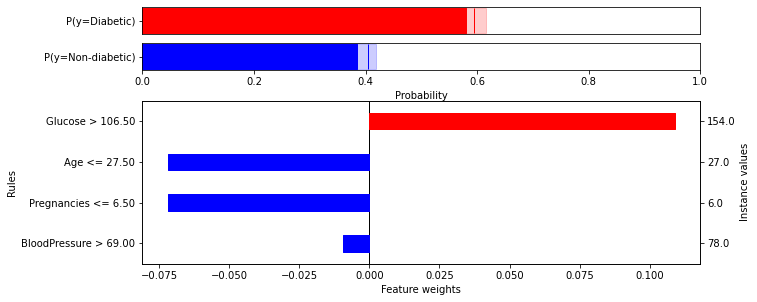
Figure 1: Regular CE plot with continuous feature values from the data set Diabetes.

Figure 1 shows a regular CE plot from the diabetes data set with a calibrated probability estimate of about $0.6$ for the positive class, indicating that the patient should be classified as diabetic (shown by the two bars at the top). The main plot visualizes the feature weights, the solid black line at $0$ the calibrated probability estimate , indicated by the solid line in the P(y=Diabetic) bar. Among the different features, one feature clearly contribute positively towards the patient being diabetic whereas the remaining three features contribute towards the patient being non-diabetic. In the given example, the feature Glucose influence the prediction the most, with a weight of $0.11$ in favour of diabetic, as long as the feature value stays above $106.5$. Age and Pregnancies are the second and third most influential features, where the low age and the number of pregnancies being less than $6.5$ both influence the prediction towards non-diabetic with about $0.07$. BloodPressure is the fourth feature that is identified as having an impact on the prediction, also favoring non-diabetic. The ambiguous prediction, with fairly eevn probability estimates, can be understood from the fact that the weights point in opposite directions.

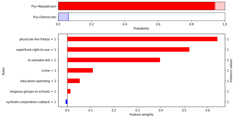
Figure 2: Regular CE plot with categorical feature values from the data set Vote.

With a data set where the features have got categorical values and a binary target (Democrat or Republican), as in figure 2, the rules look somewhat different. In the given example, the rules are either equal to $0$ $1$, with the feature values being covered by the rule. The data set is taken from results of the voting in Congress 1984, where $0$ indicated the congressman had voted negatively to a law proposal and a $1$ that the vote was positive. In the figure, the top feature physician-fee-freeze is most influential in explaining why this congressman is predicted as Republican. Almost all features favor the positive class, explaining why this prediction has a high probability estimate for the positive class.

4.1.2 With uncertainty

CE adds intervals to the plot, showing the uncertainty of the prediction narrow interval indicates certainty in the estimate or weight, and a wider interval is more uncertain in the estimate or weight. Moreover, the feature interval also shows how the feature affects the prediction estimate. igure 3 presents the explanation of the same instance as in figure 1 .

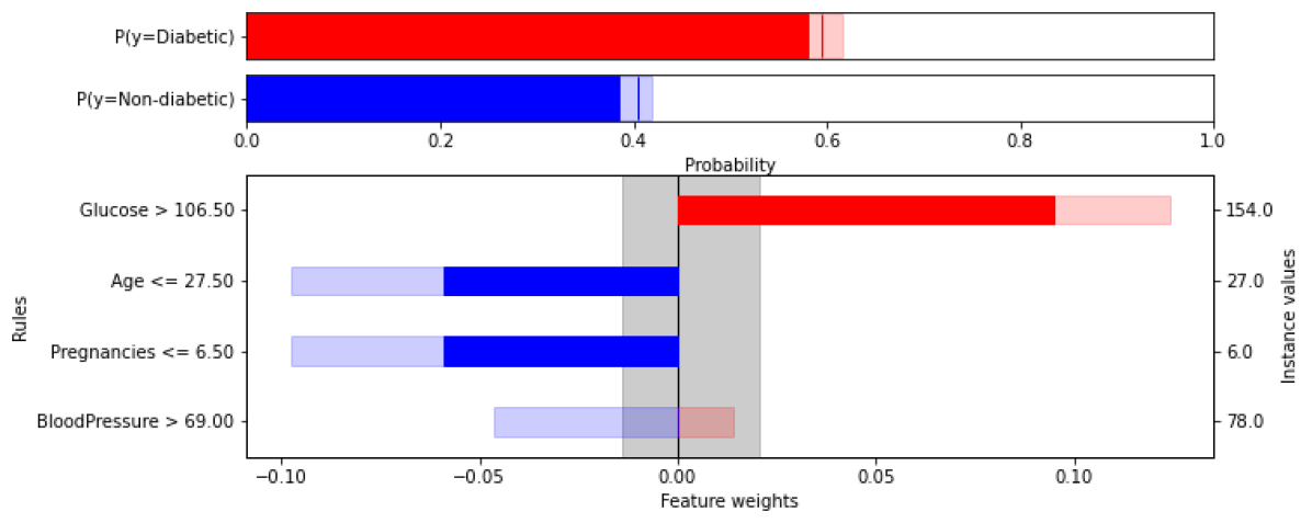
Figure 3: Uncertainty CE plot with intervals from the data set Diabetes.

The probability interval for the underlying model is indicated both in the probability bars at the top, as light blue or light red, and as the light grey area in the main part of the plot. Similarly, the feature weights are solidly coloured, from the black line, representing the calibrated probability estimate, to the lower bound of the weight interval and lightly coloured between the lower and upper bound of the interval. The rules are ordered based on the feature weights of the calibrated prediction. Blue bars indicate that the feature support the non-diabetic class, and the red bars indicate support for the diabetic class. The amount of uncertainty of the different feature weights vary slightly, with the least important feature having the most uncertainty. The uncertainty interval for BloodPressure even covers the original probability estimate, indicating an uncertainty regarding if the feature affects the prediction at all.

A different situation is seen in figure 4 where the probability of not having a liver disease is pending between the two classes. The weights point in both directions and the uncertainty intervals vary a lot. The upper bound for the mcv and sgot features are the same while the lower bound for sgot is much lower, indicating a much larger degree of uncertainty.

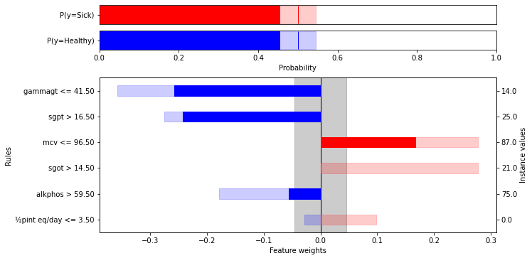
Figure 4: Uncertainty CE plot with intervals from the data set Liver.

4.2 Counterfactual Calibrated Explanations

In CCE, the plots are not showing feature weights. Instead, the plot is focusing on the VA probability intervals. Each rule shows the alternative VA probability interval resulting from perturbing the feature value to a value covered by the counterfactual rule condition.

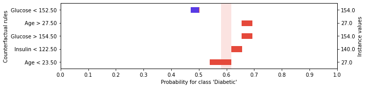
Figure 5: CCE counterfactual plot with continuous feature values from the data set Diabetes (the same instance as in figure 3).

Numerical features can, at most, result in two counterfactual rules (above or below the thresholds surrounding the feature value), whereas one counterfactual rule is created for each alternative categorical value. In the plots, only the counterfactual rules affecting the probability estimate are shown.

Like the uncertainty plot, the counterfactual plot shows that the two features Glucose and Age affect the prediction most. However, in the plot, the rules show that even a small reduction in the Glucose feature (Glucose $<152.5$) may change the probability estimate enough to change the prediction of the model. Higher Age and Glucose will increase the likelyhood for the patient being diabetic.

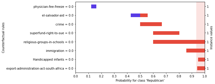
Figure 6: CE counterfactual plot with categorical feature values from the data set Vote.

In figure 6, the chosen instance is the same as in figure 2 with a clear prediction of the congressman being a Republican. There are some interesting features to point out for this instance. First, just as seen earlier in figure 2, the physician-fee-freeze feature is highly important for the prediction and changing the value according to the counterfactual rule would modify the prediction. The second counterfactual rule would decrease the certainty dramatically without clearly indicating whether the model would predict it as Democrat or Republican. Several of the remaining counterfactual rules also affect the probability and uncertainty a lot but without changing the prediction.

5 Experiments

5.1 Experimental Setup

In order to verify some of the claims of CE, two experiments have been run. The two experiments evaluate the stability and the robustness of the method. Stability is evaluated through experiments where the same model, calibration set and test set have been explained 30 times per data set. The only source of variation was the random seed. Robustness is evaluated through experiments where training and calibration sets have been randomly resampled before a new model was trained and explained. The experiment where run 30 times per data set with the same test set for all runs. A test set with 20 stratified instances (making sure both classes being equally represented) were used. Robustness is measured in this way to avoid inferring perturbed instances which are not from the same distribution as the test instances being explained. The probability estimate of each of the models was computed on the same test set, as comparison to the robustness results. The expectation is that a stable and robust explanation method should result in low variance in the feature weights. Both random forests and xGBoost are used and both factual and counterfactual explanations are evaluated.

$25$ binary classification problems were used, publicly available from either the UCI repository [Dua & Graff, 2017] or the PROMISE Software Engineering Repository [Sayyad Shirabad & Menzies, 2005]. The data set’s characteristics are presented in Table 1, where #inst. is the number of instances and #attrib. is the number of input attributes. Attributes with less than $10$ unique values were treated as categorical attributes.

Table 1: Data set characteristics

Name	#inst.	#attrib.	Name	#inst.	#attrib.
colic	357	60	kc2	369	22
creditA	690	43	kc3	325	40
diabetes	768	9	liver	341	7
german	955	28	pc1req	104	9
haberman	283	4	pc4	1343	38
heartC	302	23	sonar	208	61
heartH	293	21	spect	218	23
Hearts	270	14	spectf	267	45
hepati	155	20	transfusion	502	5
iono	350	34	tictactoe	958	28
je4042	270	9	vote	517	17
je4243	363	9	wbc	463	10
kc1	1192	22

The code used to run the experiments are located in the evaluation folder in the repository together with supplementary material. The experiment files for this paper are named Classification_[..]_stab_rob.

5.2 Results

The results in Table 2 are the mean variance of the stability and robustness measured over the 30 runs and 20 instances. The variance is measured per instance and computed over the 30 runs on the feature weight of the most influential feature, defined as the feature most often having highest absolute feature weight. The average variance is computed over the 20 instances. The most influential feature is used since it is the feature that is most likely to be used in a decision but also the feature with the greatest expected variation (as a consequence of the weights having the highest absolute values). The Model column is the mean variance of the underlying model’s probability estimate for the robustness experiment prior to calibration.

	Stability				Robustness
	xGB		RF		xGB			RF
Dataset	CE	CCE	CE	CCE	CE	CCE	Model	CE	CCE	Model
colic	3.9e-35	3.9e-35	7.8e-33	7.8e-33	0.015	0.015	0.015	0.017	0.017	0.010
creditA	1.5e-34	1.5e-34	1.5e-32	1.5e-32	0.022	0.022	0.011	0.015	0.015	0.009
diabetes	1.2e-33	1.2e-33	5.0e-33	5.0e-33	0.017	0.017	0.014	0.015	0.015	0.013
german	1.2e-34	1.2e-34	9.6e-34	9.6e-34	0.003	0.003	0.015	0.005	0.005	0.014
haberman	5.2e-34	5.2e-34	1.2e-33	1.2e-33	0.010	0.010	0.016	0.011	0.011	0.016
heartC	0.0e+00	0.0e+00	2.7e-33	2.7e-33	0.012	0.012	0.017	0.012	0.012	0.016
heartH	2.6e-33	2.6e-33	4.9e-33	4.9e-33	0.017	0.017	0.017	0.011	0.011	0.016
heartS	1.6e-33	1.6e-33	4.3e-33	4.3e-33	0.019	0.019	0.018	0.017	0.017	0.017
hepati	1.9e-34	1.9e-34	5.2e-33	5.2e-33	0.022	0.022	0.018	0.014	0.014	0.017
iono	4.1e-35	4.1e-35	3.6e-33	3.6e-33	0.028	0.028	0.017	0.013	0.013	0.016
je4042	1.5e-33	1.5e-33	6.4e-33	6.4e-33	0.018	0.018	0.017	0.015	0.015	0.017
je4243	5.3e-34	5.3e-34	5.0e-33	5.0e-33	0.010	0.010	0.018	0.010	0.010	0.017
kc1	5.4e-34	5.4e-34	1.7e-33	1.7e-33	0.011	0.011	0.017	0.009	0.009	0.017
kc2	7.7e-34	7.7e-34	5.0e-34	5.0e-34	0.018	0.018	0.018	0.007	0.007	0.017
kc3	1.4e-35	1.4e-35	5.7e-34	5.7e-34	0.007	0.007	0.017	0.005	0.005	0.017
liver	2.2e-33	2.2e-33	8.7e-33	8.7e-33	0.025	0.025	0.017	0.030	0.030	0.017
pc1req	7.7e-35	7.7e-35	1.8e-33	1.8e-33	0.014	0.014	0.018	0.014	0.014	0.017
pc4	3.7e-34	3.7e-34	2.5e-33	2.5e-33	0.009	0.009	0.017	0.007	0.007	0.017
sonar	1.8e-34	1.8e-34	2.2e-33	2.2e-33	0.019	0.019	0.017	0.009	0.009	0.017
spect	0.0e+00	0.0e+00	1.5e-33	1.5e-33	0.007	0.007	0.017	0.006	0.006	0.016
spectf	4.6e-34	4.6e-34	4.2e-34	4.2e-34	0.006	0.006	0.016	0.005	0.005	0.016
transfusion	2.8e-34	2.8e-34	2.9e-33	2.9e-33	0.009	0.009	0.017	0.008	0.008	0.017
ttt	0.0e+00	0.0e+00	4.2e-32	4.2e-32	0.017	0.017	0.016	0.025	0.025	0.016
vote	0.0e+00	0.0e+00	6.5e-33	6.5e-33	0.014	0.014	0.016	0.011	0.011	0.016
wbc	5.7e-33	5.7e-33	2.5e-33	2.5e-33	0.021	0.021	0.016	0.018	0.018	0.015
Average	7.6e-34	7.6e-34	5.4e-33	5.4e-33	0.015	0.015	0.016	0.012	0.012	0.016

Table 2: Stability and Robustness

As can be seen Table 2, the stability is practically $0$ for both factual CE (CE) and counterfactual CE (CCE), illustrating that the method is stable by definition. The minuscule variations stem from the different random seeds, having a negligible impact.

The robustness is also low, even if the mean variance robustness is clearly larger than for stability. The robustness is comparable to the variance of the probability estimates used as reference. This indicates that the method is fairly robust to perturbations such as variations of the calibration set and the model. Obviously, since the method is explaining the calibrated probability estimates of the model, it must be expected that the method is sensitive to changes to the probability estimates.

6 Discussion

6.1 Characteristics of Calibrated Explanations

One of the most important characteristics of a good explanation method is that it must be reliable. When it comes to XAI methods, reliability most often refers to its fidelity to the model being explained. However, if the model in itself is not reliable, i.e., if it is poorly calibrated and thus misrepresents reality, high fidelity is more likely to convey harm than benefit. Consequently, to create reliable explanations, the explanation must have high fidelity to a model which is well-calibrated. In addition, there is yet another layer to reliability which relates to uncertainty. For an explanation to be truly reliable, the explanation must be able to convey insights into when the model is making a prediction in which it has high confidence contra when it has low confidence. This goes beyond the model having high or low probability estimates, since the probability estimate may be high, but the model may not have seen many similar cases and thus have low confidence in the prediction, and vice versa. The main strength of the proposed method is that it provides high reliability with regard to all three layers of reliability.

• The model is calibrated to ensure an accurate reflection of reality. This includes uncertainty quantification of the model’s probability estimates.

• The explanations have high fidelity with feature weights exactly defined in relation to the calibrated probability estimates of the model. The feature weights are also calibrated to ensure fidelity.

• The method produces uncertainty quantification of the feature weights that provide insights about the degree of confidence to put in each weight. For the counterfactual explanations, the method instead provide uncertainty quantification about the estimated probability interval.

Stability is, as mentioned earlier, a critical aspect of an explanation method and something that primarily LIME has been criticized for lacking (see, e.g., Rahnama & Boström [2019]). The method is stable by design, which is clearly shown in the experiments. The explanation generated for an instance using CE or CCE is stable as long as the same calibration set and model are used.

Another important characteristic is robustness to change. The explanations are robust by design, i.e., consistent, as long as the feature rules cover perturbations in the input values and the model prediction is not affected more than marginally. Obviously, if the model prediction is affected a lot by a perturbation, it cannot be considered a small perturbation in this context, as it has a great impact on the model and thus should also have a great impact on the explanation for the method to be reliable. The reliance on the calibration set from the same distribution as the test object will contribute to robust explanations as they will always be smoothed by the underlying distribution shared between test and calibration data. The experiment, evaluating how the method is affected by changes to calibration and model predictions, shows that the method updates its feature weights in accordance with how much the underlying model is changing its predictions.

6.2 Calibrated Explanations vs. SOTA methods

The method presented in this paper generates well-calibrated local explanations with uncertainty quantification of both the probability estimate of the model and of the feature weights. As seen in Table 3, it is only BayesSHAP and BayesLIME that share the possibilities of getting calibrated explanations and uncertainty quantification. These methods are instantiations of a Bayesian framework into SHAP and LIME rather than new methods.

None of the SOTA methods could generate both factual and counterfactual explanations (see Table 3), further highlighting the all-inclusive nature of CE. It is worth pointing out that none of the counterfactual methods were generating neither well-calibrated explanations nor uncertainty quantification.

Table 3: Characteristics of CE vs factual and counterfactual SOTA Explanation Methods [Ribeiro et al., 2016, Lundberg & Lee, 2017, Plumb et al., 2018, Ribeiro et al., 2018, Slack et al., 2021, Guidotti et al., 2018a, Karimi et al., 2020].

				Cnter		Model	Uncert.
Method	Local	Global	Factual	factual	Calibr.	agnost.	quant.
CE	X	-	X	X	X	X	X
LIME	X	-	X	-	-	X	-
SHAP	X	X	X	-	-	X	-
MAPLE	X	-	X	-	-	X	-
BayesLIME	X	-	X	-	X	X	X
BayesSHAP	X	X	X	-	X	X	X
ANCHOR	X	-	X	-	-	X	-
MACE	X	-	-	X	-	X	-
LORE	X	-	-	X	-	X	-

7 Conclusion

This paper introduces Calibrated Explanations (CE), a novel explanation method that not only calibrates the underlying model but also provides uncertainty information in the explanations. Each feature’s weight is defined by its contribution to the calibrated probability estimate for the positive class, and the explanations are conveyed through straightforward conditional rules.

CE does not stop at factual explanations; it inherently enables the creation of counterfactual rules, offering insights into the uncertainty of each counterfactual outcome. The method is available as an open-source package, installable via pip or conda, supporting the plotting of both factual and counterfactual explanations.

Two experiments evaluating the method’s robustness and stability were conducted on 25 benchmarking datasets. In the evaluations, CE demonstrated outstanding performance: effective in terms of running time, reliable due to inherent calibration and uncertainty quantification, stable with consistent calibration sets and models, and robust against small perturbations. In essence, Calibrated Explanations embody the hallmarks of a high-quality explanation method.

CE generates both factual and counterfactual explanations, which is rather unique compared to other SOTA methods. None of the methods studied in the paper could offer such a wide range of characteristics like CE: either they focus on factual or counterfactual explanations. Apart from CE, only one approach (with two instantiations) included uncertainty information and calibrated explanations.

Looking ahead, future work includes real-world scenario evaluations for user perception and support for image and text data. The evolution of the currently available plots and the introduction of additional visualization methods to enhance rule insights are also key priorities.

Competing interests

The authors acknowledge that we have no competing interests to declare.

Declaration of Generative AI and AI-assisted technologies in the writing process

During the preparation of this work the author(s) used ChatGPT, Bard and Bing Chat in order to get suggestions on how to improve and simplify descriptions and sentences. After using this tool/service, the author(s) reviewed and edited the content as needed and take(s) full responsibility for the content of the publication.

References

- Adadi & Berrada [2018] Adadi, A., & Berrada, M. (2018). Peeking inside the black-box: A survey on explainable artificial intelligence (xai). IEEE Access, 6, 52138–52160.
- Agarwal et al. [2022] Agarwal, C., Saxena, E., Krishna, S., Pawelczyk, M., Johnson, N., Puri, I., Zitnik, M., & Lakkaraju, H. (2022). Openxai: Towards a transparent evaluation of model explanations. arXiv preprint arXiv:2206.11104, .
- Alvarado-Valencia & Barrero [2014] Alvarado-Valencia, J. A., & Barrero, L. H. (2014). Reliance, trust and heuristics in judgmental forecasting. Computers in human behavior, 36, 102–113.
- Alvarez-Melis & Jaakkola [2018] Alvarez-Melis, D., & Jaakkola, T. S. (2018). On the robustness of interpretability methods. arXiv preprint arXiv:1806.08049, .
- Antorán et al. [2020] Antorán, J., Bhatt, U., Adel, T., Weller, A., & Hernández-Lobato, J. M. (2020). Getting a clue: A method for explaining uncertainty estimates. arXiv preprint arXiv:2006.06848, .
- Arrieta et al. [2020] Arrieta, A. B., Díaz-Rodríguez, N., Del Ser, J., Bennetot, A., Tabik, S., Barbado, A., García, S., Gil-López, S., Molina, D., Benjamins, R. et al. (2020). Explainable artificial intelligence (xai): Concepts, taxonomies, opportunities and challenges toward responsible ai. Information Fusion, 58, 82–115.
- Bhatt et al. [2021] Bhatt, U., Antorán, J., Zhang, Y., Liao, Q. V., Sattigeri, P., Fogliato, R., Melançon, G., Krishnan, R., Stanley, J., Tickoo, O. et al. (2021). Uncertainty as a form of transparency: Measuring, communicating, and using uncertainty. In Proceedings of the 2021 AAAI/ACM Conference on AI, Ethics, and Society (pp. 401–413).
- Buçinca et al. [2020] Buçinca, Z., Lin, P., Gajos, K. Z., & Glassman, E. L. (2020). Proxy tasks and subjective measures can be misleading in evaluating explainable ai systems. In Proceedings of the 25th international conference on intelligent user interfaces (pp. 454–464).
- Carvalho et al. [2019a] Carvalho, D. V., Pereira, E. M., & Cardoso, J. S. (2019a). Machine learning interpretability: A survey on methods and metrics. Electronics, 8, 832. URL: http://dx.doi.org/10.3390/electronics8080832. doi:10.3390/electronics8080832.
- Carvalho et al. [2019b] Carvalho, D. V., Pereira, E. M., & Cardoso, J. S. (2019b). Machine learning interpretability: A survey on methods and metrics. Electronics, 8, 832.
- Chromik & Schuessler [2020] Chromik, M., & Schuessler, M. (2020). A taxonomy for human subject evaluation of black-box explanations in xai. In ExSS-ATEC@ IUI.
- Das & Rad [2020] Das, A., & Rad, P. (2020). Opportunities and challenges in explainable artificial intelligence (xai): A survey. arXiv preprint arXiv:2006.11371, .
- David Gunning [2017] David Gunning (2017). Explainable Artificial Intelligence. Web. URL: https://www.darpa.mil/attachments/XAIProgramUpdate.pdf DARPA.
- Dimanov et al. [2020] Dimanov, B., Bhatt, U., Jamnik, M., & Weller, A. (2020). You shouldn’t trust me: Learning models which conceal unfairness from multiple explanation methods. Frontiers in Artificial Intelligence and Applications: ECAI 2020, .
- Doshi-Velez & Kim [2017] Doshi-Velez, F., & Kim, B. (2017). Towards a rigorous science of interpretable machine learning. arXiv preprint arXiv:1702.08608, .
- Dua & Graff [2017] Dua, D., & Graff, C. (2017). UCI machine learning repository. URL: http://archive.ics.uci.edu/ml.
- Grushka-Cockayne et al. [2017] Grushka-Cockayne, Y., Jose, V. R. R., & Lichtendahl Jr, K. C. (2017). Ensembles of overfit and overconfident forecasts. Management Science, 63, 1110–1130.
- Guidotti [2022] Guidotti, R. (2022). Counterfactual explanations and how to find them: literature review and benchmarking. Data Mining and Knowledge Discovery, (pp. 1–55).
- Guidotti et al. [2018a] Guidotti, R., Monreale, A., Ruggieri, S., Pedreschi, D., Turini, F., & Giannotti, F. (2018a). Local rule-based explanations of black box decision systems. arXiv:1805.10820.
- Guidotti et al. [2018b] Guidotti, R., Monreale, A., Ruggieri, S., Turini, F., Giannotti, F., & Pedreschi, D. (2018b). A survey of methods for explaining black box models. ACM computing surveys (CSUR), 51, 1--42.
- Hoffman et al. [2018] Hoffman, R. R., Mueller, S. T., Klein, G., & Litman, J. (2018). Metrics for explainable ai: Challenges and prospects. arXiv preprint arXiv:1812.04608, .
- Karimi et al. [2020] Karimi, A.-H., Barthe, G., Balle, B., & Valera, I. (2020). Model-agnostic counterfactual explanations for consequential decisions. In International Conference on Artificial Intelligence and Statistics (pp. 895--905). PMLR.
- Lambrou et al. [2015] Lambrou, A., Nouretdinov, I., & Papadopoulos, H. (2015). Inductive venn prediction. Annals of Mathematics and Artificial Intelligence, 74, 181--201.
- Löfström et al. [2022] Löfström, H., Hammar, K., & Johansson, U. (2022). A meta survey of quality evaluation criteria in explanation methods. In J. De Weerdt, & A. Polyvyanyy (Eds.), Intelligent Information Systems (pp. 55--63). Cham: Springer International Publishing.
- Lundberg & Lee [2017] Lundberg, S. M., & Lee, S.-I. (2017). A unified approach to interpreting model predictions. In Proceedings of the 31st international conference on neural information processing systems (pp. 4768--4777).
- Martens & Foster [2014] Martens, D., & Foster, P. (2014). Explaining data-driven document classifications. MIS Quaterly, 38, 73--100.
- Marx et al. [2023] Marx, C., Park, Y., Hasson, H., Wang, Y., Ermon, S., & Huan, L. (2023). But are you sure? an uncertainty-aware perspective on explainable ai. In International Conference on Artificial Intelligence and Statistics (pp. 7375--7391). PMLR.
- Molnar [2022] Molnar, C. (2022). Interpretable Machine Learning. (2nd ed.). Leanpub. URL: https://christophm.github.io/interpretable-ml-book.
- Moradi & Samwald [2021] Moradi, M., & Samwald, M. (2021). Post-hoc explanation of black-box classifiers using confident itemsets. Expert Systems with Applications, 165, 113941.
- Mothilal et al. [2020] Mothilal, R. K., Sharma, A., & Tan, C. (2020). Explaining machine learning classifiers through diverse counterfactual explanations. In Proceedings of the 2020 conference on fairness, accountability, and transparency (pp. 607--617).
- Mueller et al. [2019] Mueller, S. T., Hoffman, R. R., Clancey, W., Emrey, A., & Klein, G. (2019). Explanation in human-ai systems: A literature meta-review, synopsis of key ideas and publications, and bibliography for explainable ai. arXiv preprint arXiv:1902.01876, .
- Murdoch et al. [2019] Murdoch, W. J., Singh, C., Kumbier, K., Abbasi-Asl, R., & Yu, B. (2019). Definitions, methods, and applications in interpretable machine learning. Proceedings of the National Academy of Sciences, 116, 22071--22080.
- Parmigiani [2002] Parmigiani, G. (2002). Measuring uncertainty in complex decision analysis models. Statistical methods in medical research, 11, 513--537.
- Petej [2018] Petej, I. (2018). Small and Large Scale Probabilistic Classifiers with Guarantees of Validity. Ph.D. thesis Royal Holloway, University of London.
- Phillips-Wren & Adya [2020] Phillips-Wren, G., & Adya, M. (2020). Decision making under stress: The role of information overload, time pressure, complexity, and uncertainty. Journal of Decision Systems, 29, 213--225.
- Plumb et al. [2018] Plumb, G., Molitor, D., & Talwalkar, A. S. (2018). Model agnostic supervised local explanations. Advances in neural information processing systems, 31.
- Rahnama & Boström [2019] Rahnama, A. H. A., & Boström, H. (2019). A study of data and label shift in the lime framework. arXiv preprint arXiv:1910.14421, .
- Ribeiro et al. [2016] Ribeiro, M. T., Singh, S., & Guestrin, C. (2016). ’’Why Should I Trust You?’’: Explaining the Predictions of Any Classifier. In Proceedings of the 22nd ACM SIGKDD International Conference on Knowledge Discovery and Data Mining KDD ’16 (p. 1135–1144). New York, NY, USA: Association for Computing Machinery. doi:10.1145/2939672.2939778.
- Ribeiro et al. [2018] Ribeiro, M. T., Singh, S., & Guestrin, C. (2018). Anchors: High-precision model-agnostic explanations. In Proceedings of the AAAI conference on artificial intelligence. volume 32.
- Sayyad Shirabad & Menzies [2005] Sayyad Shirabad, J., & Menzies, T. (2005). PROMISE Repository of Software Engineering Databases. School of Information Technology and Engineering, University of Ottawa, Canada.
- Slack et al. [2021] Slack, D., Hilgard, A., Singh, S., & Lakkaraju, H. (2021). Reliable post hoc explanations: Modeling uncertainty in explainability. Advances in neural information processing systems, 34, 9391--9404.
- Van Calster et al. [2019] Van Calster, B., McLernon, D. J., Van Smeden, M., Wynants, L., & Steyerberg, E. W. (2019). Calibration: the achilles heel of predictive analytics. BMC medicine, 17, 1--7.
- Vovk et al. [2005] Vovk, V., Gammerman, A., & Shafer, G. (2005). Algorithmic Learning in a Random World. Berlin, Heidelberg: Springer-Verlag.
- Vovk & Petej [2012] Vovk, V., & Petej, I. (2012). Venn-Abers predictors. arXiv preprint arXiv:1211.0025, .
- Vovk & Petej [2014] Vovk, V., & Petej, I. (2014). Venn-abers predictors. arXiv:1211.0025.
- Vovk et al. [2015] Vovk, V., Petej, I., & Fedorova, V. (2015). Large-scale probabilistic predictors with and without guarantees of validity. arXiv:1511.00213.
- Vovk et al. [2004] Vovk, V., Shafer, G., & Nouretdinov, I. (2004). Self-calibrating probability forecasting. In Advances in Neural Information Processing Systems (pp. 1133--1140).
- Wachter et al. [2017] Wachter, S., Mittelstadt, B., & Russell, C. (2017). Counterfactual explanations without opening the black box: Automated decisions and the gdpr. Harv. JL & Tech., 31, 841.
- Wang et al. [2019] Wang, D., Yang, Q., Abdul, A., & Lim, B. Y. (2019). Designing theory-driven user-centric explainable ai. In Proceedings of the 2019 CHI Conference on Human Factors in Computing Systems CHI ’19 (p. 1–15). New York, NY, USA: Association for Computing Machinery. URL: https://doi.org/10.1145/3290605.3300831. doi:10.1145/3290605.3300831.
- Zadrozny & Elkan [2001] Zadrozny, B., & Elkan, C. (2001). Obtaining calibrated probability estimates from decision trees and naive Bayesian classifiers. In Proc. 18th International Conference on Machine Learning (pp. 609--616).
- Zhou et al. [2021a] Zhou, J., Gandomi, A. H., Chen, F., & Holzinger, A. (2021a). Evaluating the quality of machine learning explanations: A survey on methods and metrics. Electronics, 10, 593.
- Zhou et al. [2021b] Zhou, Z., Hooker, G., & Wang, F. (2021b). S-lime: Stabilized-lime for model explanation. In Proceedings of the 27th ACM SIGKDD conference on knowledge discovery & data mining (pp. 2429--2438).