Heterogeneous message passing for heterogeneous networks

Abstract

Message passing (MP) is a computational technique used to find approximate solutions to a variety of problems defined on networks. MP approximations are generally accurate in locally tree-like networks but require corrections to maintain their accuracy level in networks rich with short cycles. However, MP may already be computationally challenging on very large networks and additional costs incurred by correcting for cycles could be prohibitive. We show how the issue can be addressed. By allowing each node in the network to have its own level of approximation, one can focus on improving the accuracy of MP approaches in a targeted manner. We perform a systematic analysis of $109$ real-world networks and show that our node-based MP approximation is able to increase both the accuracy and speed of traditional MP approaches. We find that, compared to conventional MP, a heterogeneous approach based on a simple heuristic is more accurate in 81% of tested networks, faster in 64% of cases, and both more accurate and faster in 49% of cases.

I Introduction

Message passing (MP), sometimes called belief propagation or the cavity method, is a computational technique aimed at solving problems or characterizing processes on networks Newman (2022). Examples include spreading processes Karrer and Newman (2010); Lokhov et al. (2014, 2015); Altarelli et al. (2013, 2014); Bianconi et al. (2021), community detection Decelle et al. (2011); Radicchi (2018), sampling strategies Radicchi and Castellano (2018), spectral properties Dorogovtsev et al. (2003); Rogers et al. (2008), and percolation Karrer et al. (2014); Hamilton and Pryadko (2014); Radicchi and Castellano (2015); Bianconi (2017, 2018).

MP techniques are closely related to mean-field approximations Mezard and Montanari (2009); MacKay (2003), in which one relates a quantity of interest at each node to those of their neighbors. For example, the event in which someone catches an infectious disease is related to whether the people they are in contact with catch the disease. A mean-field analysis proceeds by replacing unknown quantities defined on the nodes of the network with average or expected values, (incorrectly!) assuming that these quantities are independent. One derives a set of self-consistent equations to be solved. In such mean-field approximations there is one equation for each node in the network. Unfortunately, these approximations can be inaccurate.

MP approaches follow a similar logic but at least partially account for correlations induced by edges. In place of the independence assumption of a mean-field approximation, one makes a conditional independence assumption. As for mean-field approximations, MP approximations introduce a system of self-consistent equations to be solved. Now, however, there are two equations for each edge in the network.

Conventional MP techniques are often exact on trees (networks without cycles), and are justified on general networks by a locally tree-like assumption. When applied to real networks, MP methods often generate fairly accurate predictions Melnik et al. (2011). Mistakes in the predictions can be attributed to the inability of the locally tree-like assumptions to account for the correlations introduced by cycles.

However, because many networks have a relatively high density of short cycles it is important to be able to account for them. Social networks, for instance, typically have large numbers of triangles Watts and Strogatz (1998); Newman (2010). One mechanism that would give rise to a large number of triangles is triadic closure—the process whereby two of your friends become friends with each other. Likewise shared familial, vocational, or geographical ties can lead to densely connected subgroups of individuals, and hence large numbers of triangles.

A few attempts to account for correlations due to short loops exist in the literature. Some previous methods, such as those of Refs. Newman (2009); Radicchi and Castellano (2016), do not generalize to arbitrary combinations of short loops, or suffer from the limitation of being problem specific. One promising direction is the approach of Cantwell and Newman Cantwell and Newman (2019), which accounts for correlations caused by arbitrary short loops.

The framework of Ref. Cantwell and Newman (2019) relies on a procedure for constructing appropriately defined neighborhoods around each node. We will refer to this procedure as the neighborhood message passing (NMP) approach. The size of the neighborhoods can be increased in order to improve the accuracy of the predictions, but this increase in accuracy comes at the cost of an increasingly complex set of equations to solve. The utility of NMP follows from the fact that the method provides good results for relatively small neighborhoods. The accuracy of NMP has been demonstrated for bond percolation, spectral properties of sparse matrices, and the Ising model Cantwell and Newman (2019); Kirkley et al. (2021).

However, many networks have heterogeneous degree distributions Barabási and Albert (1999), and this property may cause unique problems. First, heterogeneous degree distributions can imply a large density of short cycles Bianconi and Marsili (2005). In a random graph with $n$ nodes and degree distribution $p_{k}$, the expected number of triangles per node $\langle t\rangle$ is to leading order

$$\langle t\rangle\propto\frac{\langle k^{2}\rangle^{3}}{2n\langle k\rangle^{3}}$$ (1)

where $\langle k\rangle=\sum_{k}kp_{k}$ and $\langle k^{2}\rangle=\sum_{k}k^{2}p_{k}$. If $\langle k^{2}\rangle$ diverges as $n^{1/3}$ or faster, the expected number of triangles per node diverges, even if the network is sparse.

Second, heterogeneous degree distributions may cause MP schemes to be somewhat more computationally demanding than they are in networks with homogeneous degree distributions. By definition, each node of degree $k$ has $k$ edges. Each of these edges has a corresponding equation that typically depends on $k-1$ other variables. Evaluating these equations for a network with $n$ nodes may thus require $\mathcal{O}(n\langle k^{2}\rangle)$ operations. When $\langle k^{2}\rangle$ is large (or diverging) the numerical solution of the equations could be expensive.

Heterogeneous degree distributions may thus cause both accuracy and speed degradation for traditional MP approaches. As discussed, the NMP approach trades off speed for accuracy in networks with short cycles. For networks with relatively homogeneous degree distributions, such as social or biological networks Newman (2010), the cost may be quite acceptable. However, NMP may considerably exacerbate the speed issues caused by heterogeneous degree distributions, and the additional cost may simply be prohibitive. In this paper, we present a solution to this problem, allowing for accurate and fast approximations for real-world networks with heterogeneous degree distributions.

Our solution embraces heterogeneity and relies on an appropriately heterogeneous approximation. Large-degree nodes can be approximated by conventional mean-field approximations, since the aggregate fluctuations of their neighbors should be small by the law of large numbers. Conversely, low-degree nodes can be approximated either by conventional MP, or by NMP when there is a large density of short loops. By tailoring the level of approximation for each node we can deploy our methods to arbitrary networks.

The remaining sections of the paper are structured as follows. In Sec. II, we systematically explore the properties of neighborhoods in real-world networks, observing considerable heterogeneity. In Secs. III and IV, we first derive and then test a heterogeneous NMP approach for computing the spectral properties of real networks. We find that our approach is able to increase on both the accuracy and the speed of MP in about $50\%$ of cases. Finally, in Sec. V, we show that the NMP approach can be also used in estimating properties of the zero-field Ising model on networks, and then conclude the paper.

II Neighborhood heterogeneity

In the NMP approach, one sets a value of $r$ for the network. Given $r\geq 0$, one constructs the neighborhoods of each node, defined by a set of edges. Specifically, the $r$-neighborhood around node $i$, denoted ${E}_{i}^{r}$, consists of all edges incident to node $i$, along with all paths of length $r$ or shorter between nodes adjacent to $i$. An example of this construction is shown in Fig. 1. All nodes that appear at the end of edges in ${E}_{i}^{r}$ compose the set ${N}_{i}^{r}$. Note, $r$-neighborhoods are defined by cycles; the neighborhood ${N}_{i}^{r}$ is not equivalent to the set of nodes that are at distance $r$ from node $i$.

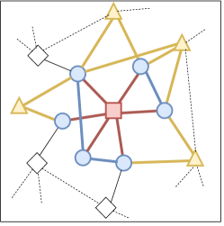
Figure 1: Definition of the $r$-neighborhood of a node. We denote the order $r$ neighborhood of node $i$ as $E_{i}^{r}$. Neighborhoods are naturally defined in terms of edges; the set of nodes that are in the neighborhood, i.e., $N_{i}^{r}$, is composed of all nodes at the end of at least one edge in $E_{i}^{r}$. For the focal node $i$, shown as a red square in the figure, the neighborhood $E_{i}^{0}$ consists of all edges incident to the node, depicted in red (edges between the square and the circles). For $E_{i}^{1}$, the neighborhood consists of all edges in $E_{i}^{0}$ along with all edges between neighbors of $i$, depicted in blue (edges between circles). For $E_{i}^{2}$, the neighborhood consists of all edges in $E_{i}^{1}$ along with all edges on paths of length two neighbors of $i$, depicted in yellow (edges between circles and triangles). Nodes in the neighborhoods $N_{i}^{0}$ and $N_{i}^{1}$ are denoted by blue circles; $N_{i}^{2}$ is composed of all nodes denoted as either blue circles or yellow triangles.

To begin, we compute the size of the neighborhoods of $109$ real-world networks. Percolation properties of these networks have been investigated in Refs. Radicchi (2015); Radicchi and Castellano (2015, 2016). The corpus contains networks of different nature, including technological, biological, social, and information networks. See Tables 1- 3 for details. All networks in the corpus are relatively sparse. Other structural properties—e.g., size, clustering coefficient, average length, degree distribution and degree correlations—vary greatly within the corpus.

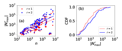
Figure 2: Size of the largest neighborhoods in real-world networks. (a) We consider $109$ real-world networks. For each network, we evaluate the size of the largest neighborhood $|N_{\max}^{r}|$ and plot it as a function of the size $n$ of the network. Each point in the plot refers to a network. The lines are power-law fits of the data points, i.e., $|N_{\max}^{r}|\sim n^{\beta^{r}}$. The best fit is obtained using linear regression on the logarithms of the data. We find $\beta^{1}=0.57$ (Pearson’ s linear correlation coefficient $0.69$) and $\beta^{2}=0.67$ $(0.71)$. (b) Cumulative distribution function (CDF) of $\left|N^{r}_{\max}\right|$. Data are the same as in panel (a).

To get a sense of how the NMP approximation will scale, we look at the dependence of the size of the largest neighborhood, i.e., $|N_{\max}^{r}|=\max_{i}|N_{i}^{r}|$, with the network size. Our results, reported in Fig. 2, indicate that the size of the largest neighborhood grows with the network size. There are a few networks for which the largest neighborhood are very small compared to the network size. This is the case of networks with homogeneous degree distributions and/or strong spatial embedding, as for example road networks. Networks with heterogeneous degree distributions are instead characterized by large neighborhoods. To give quantitative references, we find that for $50\%$ of the networks, $\left|N^{2}_{\max}\right|\geq 0.22\,n$.

In summary, these results show that some networks contain large neighborhoods. If the NMP equations scale poorly with the neighborhood size then the approach will be infeasible. In the next section, we remedy this by adjusting $r$ at the level of individual nodes.

III Heterogeneous message passing

III.1 General approach

In the NMP approach of Cantwell and Newman (2019) one chooses a single value of $r$. Using the neighborhoods, and specific to the problem at hand, one derives a set of MP equations of the form

$$H_{i} =\Phi_{i}\big{(}\bm{H}_{i\leftarrow N_{i}^{r}}\big{)}$$ (2)

$$H_{i\leftarrow j} =\Phi_{i\leftarrow j}\big{(}\bm{H}_{i\leftarrow N_{j}^{r}\setminus N_{i}^{r}}\big{)}\;,$$ (3)

where $\bm{H}_{i\leftarrow N_{i}^{r}}$ is the vector of $H_{i\leftarrow j}$ for $j\in N_{i}^{r}$, and $\Phi_{i}$ and $\Phi_{i\leftarrow j}$ are problem-specific MP functions. A MP algorithm consists of initializing the variables (e.g., at random) and then iterating this set of equations until they converge to a fixed point. In general, convergence may not be mathematically guaranteed; necessary and sufficient conditions for convergence are unclear, but this does not appear to be a significant problem in practice Weiss (2000); Zivan et al. (2020). When setting $r=0$, these equations reduce to the conventional MP ones. Increasing $r$ should increase the accuracy of the approach, but potentially with a considerable increase of the computational cost.

As discussed, in a heterogeneous network there may be competing considerations on how to appropriately set the value of $r$. For example, in a sparse network with a high density of short cycles, we are likely to require $r\geq 1$ for an accurate approximation. On the other hand, heterogeneous degree distributions may even increase the cost to solving the traditional MP equations. Further increasing the complexity of the equations to be solved by increasing $r$ may simply be untenable. How should one proceed?

Our solution is based on the simple observation that the neighborhood formalism does not actually require that each neighborhood is constructed with the same value of $r$. Around nodes that are dense with short cycles but have relatively low degree, we can increase $r$. This increases accuracy with only a small increase to computational cost. Conversely, for nodes with very high degrees, we can decrease $r$ to reduce computational burden without a significant decrease in accuracy. In fact, for nodes with extremely high degree we should find $H_{i\leftarrow j}\approx H_{j}$, i.e., that the messages have the same numerical value as the marginals. Making this approximation corresponds to a mean-field approximation, and helps to further reduce the computational cost caused by high-degree nodes.

We allow each node $i$ to have its own approximation value $r_{i}$. Re-writing the NMP equations but with heterogeneous $r$ we get

$$H_{i} =\Phi_{i}\big{(}\bm{H}_{i\leftarrow N_{i}^{r_{i}}}\big{)}$$ (4)

$$H_{i\leftarrow j} =\begin{cases}\,H_{j}\quad&\text{if }r_{j}=-1\\ \,\Phi_{i\leftarrow j}\big{(}\bm{H}_{i\leftarrow N_{j}^{r_{j}}\setminus N_{i}^{r_{i}}}\big{)}\quad&\text{if }r_{j}\geq 0.\end{cases}$$ (5)

Note we allow $r_{j}=-1$ and use this notation to indicate the standard mean-field approximation.

Below, we test the ability of heterogeneous NMP to account for the spectral properties of large networks. We find that increasing $r$ does indeed increase the accuracy of the approach over conventional MP, at the expense of increased compute time. However, by setting $r_{i}=0$ for large-degree nodes, we retain much of the improved accuracy for only a small additional cost compared to conventional MP. Remarkably, by setting $r_{i}=-1$ for the large-degree nodes, we find it is possible to derive an algorithm that is able to improve on both accuracy and speed, compared to conventional MP.

III.2 Spectral density estimation

As a specific application, we consider an heterogeneous NMP approximation for the estimation of the spectral density of the graph operators, e.g., adjacency matrix, graph Laplacian. The spectral density of matrix $\bm{M}$ with eigenvalues $\lambda_{k}$ is defined

$$\rho(z)=-{1\over n\pi}\sum_{k=1}^{n}{1\over z-\lambda_{k}}$$ (6)

for complex $z$.

Following Ref. Cantwell and Newman (2019), one can approximate $\rho(z)$ by first solving the MP equations

$$H_{i}(z)=\sum_{w\in W_{i}}|w|\prod_{j\in w}{1\over z-H_{i\leftarrow j}(z)}$$ (7)

$$H_{i\leftarrow j}(z)=\sum_{w\in W_{j\setminus i}}|w|\prod_{k\in w}{1\over z-H_{j\leftarrow k}(z)}\;,$$ (8)

where the sum is over all closed walks $w$ in the neighborhood $N^{0}_{i}$ or $N^{0}_{j}\setminus N^{0}_{i}$ respectively, and $|w|$ is the product of all edges in the walk. These equations can be solved relatively efficiently using matrix algebra—see Cantwell and Newman (2019)—and finally one approximates

$$\rho(z)=-{1\over n\pi}\sum_{i=1}^{n}{1\over z-H_{i}(z)}\;.$$ (9)

In the NMP heterogeneous approximation, we mostly leave the equations unchanged, except that now we allow the neighborhood $N^{r_{i}}_{i}$ of node $i$ to be defined with its own value of $r_{i}$, and also allow for the mean-field approximation if $r_{i}=-1$,

$$H_{i\leftarrow j}(z)=\begin{cases}H_{j}(z)\quad&r_{j}=-1\\ {\sum_{w\in W_{j\setminus i}}}|w|{\prod_{k\in w}}{1\over z-H_{j\leftarrow k}(z)}\quad&r_{j}\geq 0.\end{cases}$$ (10)

To establish the desired value of $r_{i}$ for each node $i$, we set parameters $r_{\text{min}}$, $r_{\text{max}}$, and $K$. The value of $r_{i}$ is chosen to be the largest value $r_{\text{min}}\leq r_{i}\leq r_{\text{max}}$ so that $\big{|}N_{i}^{r_{i}}\big{|}\leq K$. This procedure imposes $r_{i}=r_{\text{min}}$ whenever the degree of node $i$ is larger than $K$. Otherwise, it imposes $r_{i}$ as large as possible so that the neighborhood contains no more than $K$ nodes.

IV Numerical results

We estimate the spectral density of the graph Laplacian of the real networks in our corpus. The spectral properties of the Laplacian are important for many graph applications, including graph invariants (e.g., connectivity, expanding properties, genus, diameter, mean distance and chromatic number), partition problems (e.g, graph bisection, connectivity and separation, isoperimetric numbers, maximum cut, clustering, graph partition), and optimization problems (e.g., cutwidth, bandwidth, min-p-sum problems, ranking, scaling, quadratic assignment problem) merris94 ; chung03 ; chung97 ; biyikoglu07 . We estimate the ground-truth density, namely $\rho(z)$, using the standard numerical library LAPACK lap . This method requires a time that scales as the cube of the network size.

NMP approximations, denoted with $\tilde{\rho}(z)$, are instead obtained numerically solving Eqs. (9-10). We consider different levels of approximations. We always set $r_{\min}=-1$; we consider $r_{\max}=0$, $r_{\max}=1$ and $r_{\max}=2$; we vary the value of the parameter $K$. For $K=N\geq|N_{\max}^{r}|$, no heterogeneous approximation is de facto implemented, and the above approach reduces to the one already considered in Ref. Cantwell and Newman (2019).

The densities $\rho(z)$ and $\tilde{\rho}(z)$ are computed for $z\in[0,10]$ and with a resolution $dz=0.2$. In particular, we normalize the densities within the interval $[0,10]$. In the NMP approximations, we use $\epsilon=0.1$ as the value of the broadening parameter, see Ref.  Cantwell and Newman (2019) for details. All numerical tests are performed on a server with Intel(R) Xeon(R) CPU E5-2690 v4 @ 2.60GHz CPUs and $378$ GB of RAM.

Not all the networks in our corpus are part of the analysis. For $K=N$, we consider only networks with a number of nodes $N\leq 20,000$. For $K=10$, we consider all networks with size $N\leq 100,000$. Irrespective of the level of the approximation, we let the algorithm run for up to seven days on our machine. For the slowest NMP approximation, i.e., $r_{\max}=2$ and $K=N$, we were able to estimate the spectral density of the graph Laplacian only for $41$ networks. For faster approximations, the number of analyzed networks was higher. Details are provided in Tables 1- 3.

We first focus our attention on how the time required for the estimation of the spectral density of the graph Laplacian using the NMP approximations scales with size of the network and the size of the largest neighborhood in the network.

Results for $K=N$ are presented in Fig. 3. The relation between computational time $T^{r}$ and network size $n$ is not very neat (Fig. 3a). However, $T^{r}$ grows power like with $\left|N^{r}_{\max}\right|$ in a clear manner (Fig. 3b). The measured exponents are all in line with the expected complexity of the matrix inversion algorithm used to estimate messages within individual neighborhoods Cantwell and Newman (2019). In fact, the inversion algorithm scales cubically with the matrix dimension, thus the computational time of the entire algorithm is dominated by the inversion of the matrix associated with the largest neighborhood in the graph.

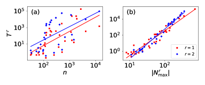
Figure 3: Computational time for the estimation of the spectral density of the graph Laplacian. We consider a subset of the $109$ real-world networks at our disposal. For each network, we measure the computational time $T^{r}$ required by the NMP algorithm for the computation of the spectral density of the graph Laplacian. Estimates of $T^{r}$ are given in seconds. (a) We plot $T^{r}$ as a function of the network size $n$. The lines are power-law fits of the data points, i.e., $T^{r}\sim n^{\tau^{r}}$. Fits are obtained using simple linear regression between the log-transformed variables. We find $\tau^{1}=1.21$ (Pearson linear correlation coefficient $0.64$) and $\tau^{2}=1.32(0.48)$. (b) We consider the same networks as in panel (a), but we test the scaling $T^{r}\sim|N_{\text{max}}^{r}|^{\sigma^{r}}$. We find $\sigma^{1}=2.99(0.96)$ and $\sigma^{2}=3.56(0.98)$.

Results for $K=10$ are presented in Fig. 4. The relation between computational time $\tilde{T}^{r}$ and network size $n$ is clearly linear (Fig. 4a). $\tilde{T}^{r}$ now grows sub-linearly with $\left|N^{r}_{\max}\right|$, however, the relationship is not as clear as the one that relates $\tilde{T}^{r}$ to $n$ (Fig. 4b).

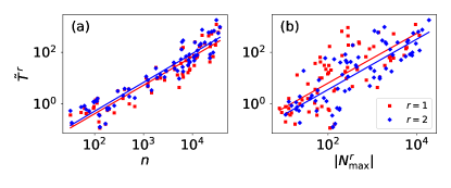
Figure 4: Computational time for the estimation of the spectral density of the graph Laplacian under the heterogeneous approximation. We consider a subset of the $109$ real-world networks at our disposal. For each network, we measure the computational time $\tilde{T}^{r}$ required by the NMP algorithm for the computation of the spectral density of the graph Laplacian. Estimates of $\tilde{T}^{r}$ are given in seconds. (a) We plot $\tilde{T}^{r}$ as a function of the network size $n$. The lines are power-law fits of the data points, i.e., $\tilde{T}^{r}\sim n^{\tilde{\tau}^{r}}$. We find $\tilde{\tau}^{1}=0.98$ (Pearson linear correlation coefficient $0.93$) and $\tilde{\tau}^{2}=1.00(0.94)$. (b) We consider the same networks as in panel (a), but we test the scaling $\tilde{T}^{r}\sim|N_{\text{max}}^{r}|^{\tilde{\sigma}^{r}}$. We find $\tilde{\sigma}^{1}=0.80(0.66)$ and $\tilde{\sigma}^{2}=0.81(0.72)$.

In Fig. 5, we compare the ground-truth spectral density with NMP-based estimates obtained at different levels of approximation. Here, we set $r_{\min}=-1$ and $r_{\max}=2$, and we vary $K$ to control for the level of the approximation. The comparison is made for two real-world networks. For small $K$ values, the approximate spectral density fails to properly capture the behavior of the ground-truth density. The accuracy greatly improves as $K$ is increased if $K$ is small. For sufficiently large values of $K$, no visible changes are apparent in the estimated densities. For example, already for $K=10$ the approximate density appears almost identical to the one obtained for $K=N$.

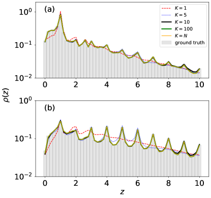
Figure 5: Laplacian spectral density of real-world networks. (a) Spectral density of the graph Laplacian $\rho(z)$ for the network of users of the Pretty-Good-Privacy algorithm for secure information interchange Boguñá et al. (2004). The various approximations are obtained by setting $r_{\min}=-1$, $r_{\max}=2$, but different $K$ values. The ground-truth density is estimated using LAPACK. (b) Same as in panel (a), but for the Cond-Mat collaboration network Newman (2001).

Figure 6: Accuracy of NMP approximations in reproducing the Laplacian spectral density of real-world networks. (a) We consider a subset of the $109$ real-world networks at our disposal. For each network, we estimate the Hellinger distance between the ground-truth Laplacian spectral $\rho(z)$ and its approximation $\tilde{\rho}(z)$ obtained via NMP. In all approximations, we set $r_{\min}=-1$. We vary instead the values of $r_{\max}$ and $K$. For each approximation, we plot the cumulative distribution function (CDF) of the Hellinger distance over the set of analyzed networks. (b) For each network, we estimate the Hellinger distance between the NMP approximations obtained for $K=10$ and $K=N$. Results of the experiments are obtained for $r_{\min}=-1$. We consider the cases $r_{\max}=1$ and $r_{\max}=2$.

We test systematically the above two observations in the corpus of real networks. To compare two spectral densities, we make use of the Hellinger distance, i.e.,

$$d(\rho,\tilde{\rho})=1-\int_{0}^{10}\,dz\sqrt{\rho(z)\tilde{\rho}(z)}.$$ (11)

By definition, we have $0\leq d(\rho,\tilde{\rho})\leq 1$, with $d=0$ indicating perfect agreement between $\rho$ and $\tilde{\rho}$. In Fig. 6a, we display the cumulative distribution of the Hellinger distance obtained over a subset of networks in our corpus. Comparisons are made between the ground-truth density and different types of approximations. All NMP-based approximations are generally good. The accuracy of the approximation increases if we increase $r_{\max}=1$ to $r_{\max}=2$, and also we increase $K=10$ to $K=N$. However, the change in accuracy is not that dramatic. Indeed, for a fixed value of $r_{\max}$, increasing $K=10$ to $K=N$ generates little changes in the predicted distribution as apparent from the results of Fig. 6b. For $75\%$ of the networks, the increase $K=10\to K=N$ induces a change in the predicted distribution corresponding to a value of the Hellinger distance smaller than $0.01$.

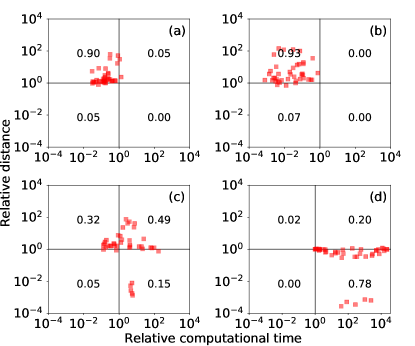
Figure 7: Trade off between time and accuracy in approximating the Laplacian spectral density of real-world networks. (a) We consider the same subset of real-networks as in Fig. 6. Each point denotes a network. For each network, we estimate the Hellinger distances between the ground-truth Laplacian spectral density and two NMP approximations, namely approximations $a$ and $b$, obtained for $r_{\max}=r^{(a)}_{\max}=0$, $K=K^{(a)}=N$ and $r_{\max}=r^{(b)}_{\max}=1$, $K=K^{(b)}=N$, respectively. We also measure the computation time required by the approximations. We then plot the ratio between the Hellinger distances of two approximations as a function of the ratio of their computational time. To facilitate the interpretation of the plot, we divided it into four quadrants. The left quadrants denote the region where approximation $a$ is slower than approximation $b$; the top quadrants indicate that approximation $a$ is less accurate than approximation $b$. We also report the fraction of networks observed in each of the four quadrants. (b) Same as in (a), but for $r^{(a)}_{\max}=0$, $K=K^{(a)}=N$ and $r^{(b)}_{\max}=2$ and $K=K^{(b)}=N$. (c) Same as in (a), but for $r^{(a)}_{\max}=0$, $K=K^{(a)}=N$ and $r^{(b)}_{\max}=2$ and $K=K^{(b)}=10$. (d) Same as in (a), but for $r^{(a)}_{\max}=2$, $K=K^{(a)}=N$ and $r^{(b)}_{\max}=2$ and $K=K^{(b)}=10$.

We complete the summary of our analysis in Fig. 7. There, we compare different levels of approximations in terms of accuracy and computational time. As expected, we find that increasing $r_{\max}$ while keeping $K$ fixed leads to an increase of accuracy and computational time (Figs. 7a and  7b). Only a few exceptions are visible; these are given by very small networks, with sizes $n\leq 100$. Quite surprisingly, we find that, for $49\%$ of the analyzed networks, the proposed heterogeneous NMP approximation is faster and more accurate than the standard MP approximation (Fig. 7c). For many small networks, their performance is similar and is obtained in a similar time. The only apparent exceptions are given by five distinct snapshots of the peer-to-peer Gnutella network Ripeanu et al. (2002); Leskovec et al. (2007a), where the MP approximation greatly outperforms the NMP approximation, but with a computational time that is about two orders of magnitude larger than the NMP approximation. Finally, we confirm that the accuracy of the NMP approximation obtained for $r_{\max}=2$ and $K=10$ is almost identical to the one achieved for $r_{\max}=2$ and $K=N$ (Fig. 7c). The only exceptions are still given by the five Gnutella networks. However, the greater accuracy is achieved thanks to a significant increase in computational time.

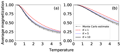
Figure 8: Heterogeneous belief propagation for the zero-field Ising model. (a) Average magnetization of the zero-field Ising model for the Pretty-Good-Privacy network Boguñá et al. (2004). Results are obtained by integrating the heterogeneous NMP equations of Eqs. (4) and (5) with the belief propagation framework of Kirkley et al. (2021). The various curves are obtained by setting $r_{\min}=-1$, $r_{\max}=2$, but allowing $K$ to range over multiple different values. The ground-truth magnetization is estimated using the Wolff cluster MCMC algorithm. (b) Same as in panel (a), but for the Cond-Mat collaboration network Newman (2001).

V Discussion

We systematically tested the NMP approach on a corpus of $109$ networks. We found, in accordance with expectations, that increasing the cycles accounted for by increasing $r$ led to improved accuracy at the expense of speed.

We also introduced a hybrid approach, that uses more accurate approximations for low-degree nodes, and less accurate mean-field approximations at very high-degree nodes. We tested the hybrid approach in estimating the spectral density of the graph Laplacian of the real networks in our corpus. Compared to conventional MP, this approach was more accurate in 81% of networks (Fig. 7(c): $0.49+0.32=0.81$). In addition, it was also faster in 64% of cases (Fig. 7(c): $0.49+0.15=0.64$). In a plurality of cases, the approximation was both faster and more accurate than conventional MP. The findings suggest that the NMP framework is applicable to a wide class of networks, even those with very large hubs.

The proposed NMP approach can be used in other problems whose solution can be approximated via conventional MP. Our detailed numerical experiments have focused on spectral density, a problem with ground truth that can be computed numerically for relatively large networks. However, as a final example, we consider the belief propagation framework of Kirkley et al. (2021) to compute the magnetization of the zero-field Ising model. Fig. 8 shows the magnetization for $r_{\min}=-1$, $r_{\max}=2$ and different values of $K$, for the same networks analyzed in Fig. 5. We see that as we increase $K$ we get improved approximations of the magnetization, and that for $K=10$ the results are quite close to Monte Carlo estimates.

In summary, we find that heterogeneous message passing approximations are effective for heterogeneous networks. Specifically, high-degree nodes can be well accounted for with conventional mean-field approaches, while the corrections due to cycles are incorporated in the lower-degree nodes. Both speed and accuracy can be simultaneously improved by applying appropriate approximations.

Network	Ref.	URL	$N$	$E$	$\left|N^{1}_{\max}\right|$	$\left|N^{2}_{\max}\right|$	$T^{1}$	$T^{2}$	$\tilde{T}^{1}$	$\tilde{T}^{2}$
*Social 3	Milo et al. (2004)	url	$32$	$80$	$14$	$22$	$0$	$1$	$0$	$0$
*Karate club	Zachary (1977)	url	$34$	$78$	$18$	$23$	$0$	$0$	$0$	$0$
*Protein 2	Milo et al. (2004)	url	$53$	$123$	$8$	$19$	$0$	$1$	$0$	$0$
*Dolphins	Lusseau et al. (2003)	url	$62$	$159$	$12$	$26$	$0$	$3$	$0$	$0$
*Social 1	Milo et al. (2004)	url	$67$	$142$	$11$	$18$	$0$	$1$	$0$	$0$
*Les Miserables	Knuth (1993)	url	$77$	$254$	$36$	$55$	$2$	$9$	$0$	$0$
*Protein 1	Milo et al. (2004)	url	$95$	$213$	$7$	$12$	$0$	$1$	$0$	$1$
*E. Coli, transcription	Mangan and Alon (2003)	url	$97$	$212$	$11$	$18$	$0$	$1$	$0$	$1$
*Political books	Adamic and Glance (2005)	url	$105$	$441$	$25$	$51$	$7$	$62$	$1$	$1$
*David Copperfield	Newman (2006)	url	$112$	$425$	$50$	$92$	$13$	$227$	$1$	$1$
*College football	Girvan and Newman (2002)	url	$115$	$613$	$13$	$39$	$5$	$39$	$1$	$1$
*S 208	Milo et al. (2004)	url	$122$	$189$	$10$	$10$	$0$	$0$	$0$	$0$
*High school, 2011	Fournet and Barrat (2014)	url	$126$	$1,709$	$56$	$124$	$122$	$1,824$	$0$	$0$
*Bay Dry	Ulanowicz et al. (1998); Kunegis (2013)	url	$128$	$2,106$	$111$	$128$	$244$	$2,801$	$0$	$0$
*Bay Wet	Kunegis (2013)	url	$128$	$2,075$	$111$	$128$	$248$	$2,858$	$0$	$0$
*Radoslaw Email	Michalski et al. (2011); Kunegis (2013)	url	$167$	$3,250$	$139$	$143$	$791$	$2,371$	$0$	$0$
*High school, 2012	Fournet and Barrat (2014)	url	$180$	$2,220$	$56$	$158$	$129$	$4,681$	$0$	$0$
*Little Rock Lake	Martinez (1991); Kunegis (2013)	url	$183$	$2,434$	$105$	$180$	$413$	$4,526$	$0$	$0$
*Jazz	Gleiser and Danon (2003)	url	$198$	$2,742$	$101$	$182$	$313$	$7,915$	$0$	$0$
*S 420	Milo et al. (2004)	url	$252$	$399$	$15$	$14$	$0$	$0$	$0$	$0$
*C. Elegans, neural	Watts and Strogatz (1998)	url	$297$	$2,148$	$134$	$239$	$374$	$15,720$	$3$	$3$
*Network Science	Newman (2006)	url	$379$	$914$	$35$	$42$	$4$	$8$	$1$	$2$
*Dublin	Isella et al. (2011); Kunegis (2013)	url	$410$	$2,765$	$50$	$164$	$124$	$2,342$	$3$	$3$
*US Air Trasportation	Colizza et al. (2007)	url	$500$	$2,980$	$146$	$301$	$3,119$	$57,958$	$3$	$3$
*S 838	Milo et al. (2004)	url	$512$	$819$	$23$	$23$	$1$	$2$	$1$	$1$
*Yeast, transcription	Milo et al. (2002)	url	$662$	$1,062$	$72$	$80$	$23$	$69$	$0$	$1$
*URV email	Guimera et al. (2003)	url	$1,133$	$5,451$	$72$	$279$	$289$	$34,546$	$10$	$11$
Political blogs	Adamic and Glance (2005)	url	$1,222$	$16,714$	$351$	$867$	$24,944$	$-$	$4$	$4$
*Air traffic	Kunegis (2013)	url	$1,226$	$2,408$	$35$	$62$	$28$	$139$	$5$	$8$
*Yeast, protein	Jeong et al. (2001)	url	$1,458$	$1,948$	$57$	$57$	$16$	$34$	$2$	$3$
Petster, hamster	Kunegis (2013)	url	$1,788$	$12,476$	$272$	$904$	$24,879$	$-$	$25$	$23$
UC Irvine	Opsahl and Panzarasa (2009); Kunegis (2013)	url	$1,893$	$13,835$	$256$	$1,076$	$11,963$	$-$	$9$	$10$
Yeast, protein	Bu et al. (2003)	url	$2,224$	$6,609$	$65$	$208$	$-$	$-$	$9$	$13$
Japanese	Milo et al. (2004)	url	$2,698$	$7,995$	$726$	$1,459$	$181,172$	$-$	$8$	$10$
Open flights	Opsahl et al. (2010); Kunegis (2013)	url	$2,905$	$15,645$	$242$	$1,101$	$-$	$-$	$18$	$18$
*GR-QC, 1993-2003	Leskovec et al. (2007a)	url	$4,158$	$13,422$	$81$	$187$	$356$	$10,098$	$31$	$40$
Tennis	Radicchi (2011)	url	$4,338$	$81,865$	$452$	$2,015$	$-$	$-$	$21$	$23$

Table 1: From left to right, we report: the name of the network, the reference of the paper(s) where the network was first analyzed, the URL where the network was retrieved, the number of nodes and edges of the network, the number of nodes in the largest neighborhoods of orders $r=1$ and $r=2$, and the computational time needed to obtain the spectral density of the graph Laplacian via the NMP approximation with $r_{\max}=1$ and $K=N$, $r_{\max}=2$ and $K=N$, $r_{\max}=1$ and $K=10$, and $r_{\max}=2$ and $K=10$. The analysis was performed on the largest connected component of each network. Computational time is measured in seconds, and the reported value is rounded to the nearest integer. A computational time equal to zero seconds means that less than $0.5$ seconds were required to estimate the spectral density of the graph Laplacian. No computational time is reported for networks that could not be analyzed due to their high computational demand. The asterisk before the network name indicate that we were able to fully compute their spectrum, either exactly or using the various NMP approximations. These are the only networks included in the analysis of Figs. 6 and  7.

Network	Ref.	URL	$N$	$E$	$\left|N^{1}_{\max}\right|$	$\left|N^{2}_{\max}\right|$	$T^{1}$	$T^{2}$	$\tilde{T}^{1}$	$\tilde{T}^{2}$
US Power grid	Watts and Strogatz (1998)	url	$4,941$	$6,594$	$20$	$28$	$-$	$-$	$13$	$19$
HT09	Isella et al. (2011)	url	$5,352$	$18,481$	$1,288$	$1,464$	$-$	$-$	$4$	$9$
Hep-Th, 1995-1999	Newman (2001)	url	$5,835$	$13,815$	$50$	$136$	$-$	$-$	$36$	$53$
Reactome	Joshi-Tope et al. (2005); Kunegis (2013)	url	$5,973$	$145,778$	$855$	$2,492$	$-$	$-$	$135$	$129$
Jung	Šubelj and Bajec (2012); Kunegis (2013)	url	$6,120$	$50,290$	$5,656$	$6,050$	$-$	$-$	$137$	$250$
Gnutella, Aug. 8, 2002	Ripeanu et al. (2002); Leskovec et al. (2007a)	url	$6,299$	$20,776$	$98$	$440$	$-$	$-$	$14$	$26$
JDK	Kunegis (2013)	url	$6,434$	$53,658$	$5,923$	$6,356$	$-$	$-$	$151$	$288$
AS Oregon	Leskovec et al. (2005)	url	$6,474$	$12,572$	$1,459$	$2,685$	$-$	$-$	$10$	$18$
English	Milo et al. (2004)	url	$7,377$	$44,205$	$2,569$	$5,585$	$-$	$-$	$47$	$69$
Gnutella, Aug. 9, 2002	Ripeanu et al. (2002); Leskovec et al. (2007a)	url	$8,104$	$26,008$	$103$	$421$	$-$	$-$	$16$	$31$
French	Milo et al. (2004)	url	$8,308$	$23,832$	$1,892$	$4,405$	$-$	$-$	$30$	$50$
Hep-Th, 1993-2003	Leskovec et al. (2007a)	url	$8,638$	$24,806$	$65$	$244$	$-$	$-$	$64$	$82$
Gnutella, Aug. 6, 2002	Ripeanu et al. (2002); Leskovec et al. (2007a)	url	$8,717$	$31,525$	$115$	$266$	$-$	$-$	$20$	$40$
Gnutella, Aug. 5, 2002	Ripeanu et al. (2002); Leskovec et al. (2007a)	url	$8,842$	$31,837$	$89$	$321$	$-$	$-$	$22$	$42$
PGP	Boguñá et al. (2004)	url	$10,680$	$24,316$	$206$	$481$	$-$	$-$	$74$	$63$
Gnutella, August 4 2002	Ripeanu et al. (2002); Leskovec et al. (2007a)	url	$10,876$	$39,994$	$103$	$250$	$-$	$-$	$30$	$47$
Hep-Ph, 1993-2003	Leskovec et al. (2007a)	url	$11,204$	$117,619$	$491$	$1,960$	$-$	$-$	$247$	$242$
Spanish	Milo et al. (2004)	url	$11,558$	$43,050$	$2,986$	$7,814$	$-$	$-$	$59$	$75$
DBLP, citations	Ley (2002); Kunegis (2013)	url	$12,495$	$49,563$	$710$	$2,876$	$-$	$-$	$67$	$77$
Spanish	Kunegis (2013)	url	$12,643$	$55,019$	$5,170$	$11,524$	$-$	$-$	$75$	$117$
*Cond-Mat, 1995-1999	Newman (2001)	url	$13,861$	$44,619$	$107$	$358$	$1,478$	$98,257$	$167$	$188$
Astrophysics	Newman (2001)	url	$14,845$	$119,652$	$361$	$2,050$	$-$	$-$	$187$	$212$
Google	Palla et al. (2007)	url	$15,763$	$148,585$	$11,401$	$13,208$	$-$	$-$	$455$	$740$
AstroPhys, 1993-2003	Leskovec et al. (2007a)	url	$17,903$	$196,972$	$504$	$3,661$	$-$	$-$	$219$	$240$
Cond-Mat, 1993-2003	Leskovec et al. (2007a)	url	$21,363$	$91,286$	$280$	$1,335$	$-$	$-$	$433$	$582$
Gnutella, Aug. 25, 2002	Ripeanu et al. (2002); Leskovec et al. (2007a)	url	$22,663$	$54,693$	$67$	$85$	$-$	$-$	$42$	$59$
Internet	-	url	$22,963$	$48,436$	$2,390$	$6,954$	$-$	$-$	$62$	$82$
Thesaurus	Kiss et al. (1973); Kunegis (2013)	url	$23,132$	$297,094$	$1,062$	$9,528$	$-$	$-$	$165$	$217$
Cora	Šubelj and Bajec (2013); Kunegis (2013)	url	$23,166$	$89,157$	$377$	$818$	$-$	$-$	$-$	$-$
Linux, mailing list	Kunegis (2013)	url	$24,567$	$158,164$	$2,989$	$10,805$	$-$	$-$	$520$	$622$
AS Caida	Leskovec et al. (2005)	url	$26,475$	$53,381$	$2,629$	$7,940$	$-$	$-$	$68$	$97$
Gnutella, Aug. 24, 2002	Ripeanu et al. (2002); Leskovec et al. (2007a)	url	$26,498$	$65,359$	$355$	$860$	$-$	$-$	$-$	$-$
Hep-Th, citations	Leskovec et al. (2007a); Kunegis (2013)	url	$27,400$	$352,021$	$2,469$	$9,467$	$-$	$-$	$-$	$-$
Cond-Mat, 1995-2003	Newman (2001)	url	$27,519$	$116,181$	$202$	$1,108$	$-$	$-$	$648$	$672$
Digg	De Choudhury et al. (2009); Kunegis (2013)	url	$29,652$	$84,781$	$283$	$1,657$	$-$	$-$	$189$	$286$
Linux, soft.	Kunegis (2013)	url	$30,817$	$213,208$	$9,339$	$18,740$	$-$	$-$	$1,195$	$1,759$
Enron	Leskovec et al. (2009)	url	$33,696$	$180,811$	$1,383$	$8,264$	$-$	$-$	$590$	$550$

Table 2: Continuation of Table 1.

Network	Ref.	URL	$N$	$E$	$\left|N^{1}_{\max}\right|$	$\left|N^{2}_{\max}\right|$	$T^{1}$	$T^{2}$	$\tilde{T}^{1}$	$\tilde{T}^{2}$
Hep-Ph, citations	Leskovec et al. (2007a); Kunegis (2013)	url	$34,401$	$420,784$	$846$	$4,440$	$-$	$-$	$-$	$-$
Cond-Mat, 1995-2005	Newman (2001)	url	$36,458$	$171,735$	$278$	$1,855$	$-$	$-$	$899$	$948$
Gnutella, Aug. 30, 2002	Ripeanu et al. (2002); Leskovec et al. (2007a)	url	$36,646$	$88,303$	$56$	$86$	$-$	$-$	$-$	$-$
Slashdot	Gómez et al. (2008); Kunegis (2013)	url	$51,083$	$116,573$	$2,916$	$7,732$	$-$	$-$	$-$	$-$
Gnutella, Aug. 31, 2002	Ripeanu et al. (2002); Leskovec et al. (2007a)	url	$62,561$	$147,878$	$96$	$111$	$-$	$-$	$-$	$-$
Facebook	Viswanath et al. (2009)	url	$63,392$	$816,886$	$1,099$	$14,291$	$-$	$-$	$-$	$-$
Epinions	Richardson et al. (2003); Kunegis (2013)	url	$75,877$	$405,739$	$3,045$	$16,661$	$-$	$-$	$-$	$-$
Slashdot zoo	Kunegis et al. (2009); Kunegis (2013)	url	$79,116$	$467,731$	$2,534$	$16,810$	$-$	$-$	$-$	$-$
Flickr	McAuley and Leskovec (2012); Kunegis (2013)	url	$105,722$	$2,316,668$	$5,425$	$15,360$	$-$	$-$	$-$	$-$
Wikipedia, edits	Brandes and Lerner (2010); Kunegis (2013)	url	$113,123$	$2,025,910$	$20,153$	$72,317$	$-$	$-$	$-$	$-$
Petster, cats	Kunegis (2013)	url	$148,826$	$5,447,464$	$80,634$	$136,538$	$-$	$-$	$-$	$-$
Gowalla	Cho et al. (2011); Kunegis (2013)	url	$196,591$	$950,327$	$14,730$	$55,087$	$-$	$-$	$-$	$-$
Libimseti	Brozovsky and Petricek (2007); Kunegis et al. (2012); Kunegis (2013)	url	$220,970$	$17,233,144$	$33,390$	$181,596$	$-$	$-$	$-$	$-$
EU email	Leskovec et al. (2007a); Kunegis (2013)	url	$224,832$	$339,925$	$7,636$	$20,391$	$-$	$-$	$-$	$-$
Web Stanford	Leskovec et al. (2009)	url	$255,265$	$1,941,926$	$38,625$	$54,427$	$-$	$-$	$-$	$-$
Amazon, Mar. 2, 2003	Leskovec et al. (2007b)	url	$262,111$	$899,792$	$420$	$944$	$-$	$-$	$-$	$-$
DBLP, collaborations	Ley (2002); Kunegis (2013)	url	$317,080$	$1,049,866$	$344$	$1,431$	$-$	$-$	$-$	$-$
Web Notre Dame	Albert et al. (1999)	url	$325,729$	$1,090,108$	$10,722$	$17,682$	$-$	$-$	$-$	$-$
MathSciNet	Palla et al. (2008)	url	$332,689$	$820,644$	$496$	$2,454$	$-$	$-$	$-$	$-$
CiteSeer	Bollacker et al. (1998); Kunegis (2013)	url	$365,154$	$1,721,981$	$1,739$	$5,392$	$-$	$-$	$-$	$-$
Zhishi	Niu et al. (2011); Kunegis (2013)	url	$372,840$	$2,318,025$	$127,067$	$128,431$	$-$	$-$	$-$	$-$
Actor coll. net.	Barabási and Albert (1999); Kunegis (2013)	url	$374,511$	$15,014,839$	$3,956$	$125,645$	$-$	$-$	$-$	$-$
Amazon, Mar. 12, 2003	Leskovec et al. (2007b)	url	$400,727$	$2,349,869$	$2,747$	$6,158$	$-$	$-$	$-$	$-$
Amazon, Jun. 6, 2003	Leskovec et al. (2007b)	url	$403,364$	$2,443,311$	$2,752$	$5,738$	$-$	$-$	$-$	$-$
Amazon, May 5, 2003	Leskovec et al. (2007b)	url	$410,236$	$2,439,437$	$2,760$	$6,491$	$-$	$-$	$-$	$-$
Petster, dogs	Kunegis (2013)	url	$426,485$	$8,543,321$	$46,504$	$313,475$	$-$	$-$	$-$	$-$
Road network PA	Leskovec et al. (2009)	url	$1,087,562$	$1,541,514$	$9$	$13$	$-$	$-$	$-$	$-$
YouTube friend. net.	Yang and Leskovec (2012); Kunegis (2013)	url	$1,134,890$	$2,987,624$	$28,755$	$137,387$	$-$	$-$	$-$	$-$
Road network TX	Leskovec et al. (2009)	url	$1,351,137$	$1,879,201$	$13$	$19$	$-$	$-$	$-$	$-$
AS Skitter	Leskovec et al. (2005)	url	$1,694,616$	$11,094,209$	$35,455$	$128,203$	$-$	$-$	$-$	$-$
Road network CA	Leskovec et al. (2009)	url	$1,957,027$	$2,760,388$	$13$	$17$	$-$	$-$	$-$	$-$
Wikipedia, pages	Palla et al. (2008)	url	$2,070,367$	$42,336,614$	$230,041$	$1,640,275$	$-$	$-$	$-$	$-$
US Patents	Hall et al. (2001); Kunegis (2013)	url	$3,764,117$	$16,511,740$	$794$	$4,228$	$-$	$-$	$-$	$-$
DBpedia	Auer et al. (2007); Kunegis (2013)	url	$3,915,921$	$12,577,253$	$469,692$	$897,744$	$-$	$-$	$-$	$-$
LiveJournal	Mislove et al. (2007); Kunegis (2013)	url	$5,189,809$	$48,688,097$	$15,018$	$182,439$	$-$	$-$	$-$	$-$

Table 3: Continuation of Tables 1 and 2.