Binary Formation in a 100 $\mu$m-dark Massive Core

Abstract

We report high-resolution ALMA observations toward a massive protostellar core C1-Sa ($\sim$30 M_⊙) in the Dragon Infrared Dark Cloud. At the resolution of 140 AU, the core fragments into two kernels (C1-Sa1 and C1-Sa2) with a projected separation of $\sim$1400 AU along the elongation of C1-Sa, consistent with a Jeans length scale of $\sim$1100 AU. Radiative transfer modeling using RADEX indicates that the protostellar kernel C1-Sa1 has a temperature of $\sim$75 K and a mass of 0.55 M_⊙. C1-Sa1 also likely drives two bipolar outflows, one being parallel to the plane-of-the-sky. C1-Sa2 is not detected in line emission and does not show any outflow activity but exhibits ortho-H₂D⁺ and N₂D⁺ emission in its vicinity, thus it is likely still starless. Assuming a 20 K temperature, C1-Sa2 has a mass of 1.6 M_⊙. At a higher resolution of 96 AU, C1-Sa1 begins to show an irregular shape at the periphery, but no clear sign of multiple objects or disks. We suspect that C1-Sa1 hosts a tight binary with inclined disks and outflows. Currently, one member of the binary is actively accreting while the accretion in the other is significantly reduced. C1-Sa2 shows hints of fragmentation into two sub-kernels with similar masses, which requires further confirmation with higher sensitivity.

1 Introduction

Binary formation is an essential part of star formation, as young stellar objects usually come in pairs (or multiple systems, see Reipurth et al., 2014; Offner et al., 2022). In particular, massive stars (M $\gtrsim$ 8 M_⊙) have a remarkably high multiplicity frequency (approaching 100%, see Chini et al., 2012; Moe & Di Stefano, 2017), but their formation is still not well understood (Motte et al., 2018). Investigating the formation of massive binaries is therefore pivotal for a better understanding of massive star formation. However, statistical studies of high-mass protostars are quite challenging because the sample size is typically much smaller than that of low-mass protostars. In addition, massive protostars are typically in crowded clusters deeply embedded in molecular clouds (Zinnecker & Yorke, 2007). Observations in such regions are challenging for optical and infrared wavelengths. Statistically meaningful surveys have only started to come out within the last decade (e.g., Sana et al., 2013).

Thus far, studies of massive binary stars have not put much emphasis on the early phase (Duchêne & Kraus, 2013). However, the early phase is extremely important because the binary properties we see in later stages may be very different from that during the formation process. Therefore, to fully understand the “true” origin of massive binaries, it is crucial to focus on the very early stages of the binary formation. In particular, information about the initial separation between the binary, the mass ratio of the binary, and potentially the relative orientation of the accretion disks will be helpful for testing massive binary formation theories.

Several observations have revealed massive binary formation at the protostellar phase (e.g., Beltrán et al., 2016; Tanaka et al., 2020). Most recently, Cyganowski et al. (2022) observed a (proto)binary in a massive core that was previously thought to be prestellar, making it one of the earliest-stage forming binaries that has the potential to become massive. Such observations put stringent constraints on massive binary formation theories (e.g., Krumholz et al., 2009; Oliva & Kuiper, 2020; Mignon-Risse et al., 2021)

Star formation happens in dense molecular cores (Bergin & Tafalla, 2007). These cores provide laboratories for observing the earliest phase of binary formation. Due to the high column density toward star-forming regions and the relatively low temperature in molecular clouds, protostellar cores are best detectable at mm wavelengths (e.g.,Kong 2019; Sanhueza et al. 2019; Motte et al. 2022). For distant high-mass star-forming regions, ALMA is the best choice with its superb resolution and sensitivity. For instance, Zhang et al. (2019) used ALMA to probe a forming binary in IRAS 07299-1651 which is a massive star-forming region that is 1.7 kpc away. With a resolution of $\sim$0.03″ or $\sim$50 AU resolution, they found that the IRAS 07299-1651 binary protostar appears to be separated by $\sim$200 AU, which was interpreted as due to disk fragmentation. Additional ALMA observations that zoom into the heart of massive protostellar cores will allow future statistical studies of massive binary formation, augmenting surveys at shorter wavelengths (see, e.g., Gravity Collaboration et al., 2018) and revolutionizing our understandings of massive star formation.

Kong et al. (2018, hereafter K18) observed a massive protostellar core C1-Sa ($\sim$30 M_⊙) and an accompanying low-mass protostellar core C1-Sb ($\sim$2 M_⊙) in the Dragon infrared dark cloud (Dragon IRDC, Wang, 2018; Kong et al., 2021) with ALMA (also see Tan et al., 2016, hereafter T16). The Dragon IRDC (aka G28.34+0.06 or G28.37+0.07) is at a distance of 4.8 kpc, and the cores are embedded in a region that is dark at up to 100 $\mu$m (Ragan et al., 2012), indicating that it is at the earliest phase of star formation. With a 0.2″ spatial resolution ($\sim$960 AU at a distance of 4.8 kpc), the K18 1.3 mm continuum image showed an elongated structure in the center of C1-Sa, which hinted at the existence of two fragments (see their Figure 1) whose separation is $\sim$0.2″, i.e., the resolution limit of their ALMA data. In addition, C1-Sa likely drives two bipolar outflows. The first (hereafter C1-Sa outflow1) was identified in T16. The second (hereafter C1-Sa outflow2) was identified as a filament in T16 because the elongated structure showed up in CO channel maps contemporaneously between 74 and 80 km s^-1, i.e., it showed no blue- or red-shifted lobes. However, based on the data from Kong et al. (2019), the elongated CO structure showed well-matching SiO counterparts, indicative of a bipolar outflow, which motivated this study. The suspected binary fragmentation, if confirmed, would provide an excellent example of massive binary formation at the earliest stage.

In this paper, we present ALMA Cycle 7 high-resolution observations toward C1-Sa. We show that the core is indeed a binary system, and analyze the ALMA data to characterize its physical properties. To our knowledge, the C1-Sa binary system is the most distant proto-binary at the earliest-stage which also has the potential to become massive. It shows the very beginning of massive binary formation in an IRDC. In the following, §2, we introduce the ALMA observations and data reduction. Next, we report our findings about the binary system in §3. We discuss the implications of our results in §4. Finally, §5 summarizes and concludes the paper.

2 ALMA observations and data reduction

In this paper, we utilize multiple ALMA datasets that cover the cores. First, ALMA Cycle 2 project 2013.1.00248.S (hereafter C2) observed the area with a $\sim$0.2″ resolution. It includes the 1.3 mm continuum and CO(2-1) line, an outflow tracer. Details of the C2 data are present in T16 and K18. Second, ALMA Cycle 3 project 2015.1.00183.S (hereafter C3) mosaicked the main body of the Dragon (see Figure 1 in Kong et al., 2019) with the 1.3 mm continuum and the outflow tracers CO(2-1) and SiO(5-4). Details of the C3 data are included in Kong (2019) and Kong et al. (2019). Third, ALMA Cycle 4 project 2016.1.00988.S (hereafter C4) observed the region in ortho-H₂D⁺ (J_Ka,Kc = 1_1,0-1_1,1). The C4 data will be presented in detail in a future paper. The ortho-H₂D⁺ line data shown in this paper has a synthesized beam of $\sim 1\arcsec$ and a sensitivity of 0.015 Jy beam^-1 per 0.2 km s^-1 channel. Finally, the ALMA Cycle 7 project 2019.1.00255.S (hereafter C7) observed the C1-Sa area with a $\sim$0.03″ synthesized beam.

Here, we report the high-resolution C7 band 6 continuum and molecular line observations. A dedicated 2 GHz baseband was used for the continuum observation. The baseband was centered at 234 GHz (1.3 mm) with a channel width of 1.1 MHz. Line contamination was checked in visibilities and excluded from imaging. The continuum observation served the main goal of detecting the core fragmentation via dust emission. A spectral window for CO(2-1) was included with a 0.18 km s^-1 channel width. The line was mainly used to detect the CO outflows from the fragments in the massive C1-Sa core. We also included spectral windows for ¹³CO(2-1) and C¹⁸O(2-1) to probe the kinematics in the core. Both lines were set to a 0.19 km s^-1 spectral resolution. The rest of the spectral windows were set for CH₃CN v=0 12(1)-11(1), F=11-10 (channel width 0.18 km s^-1), H(30)$\alpha$ (channel width 0.18 km s^-1), SO 3$\Sigma$ v=0 6(5)-5(4) (channel width 0.18 km s^-1), SiO(5-4) (channel width 0.39 km s^-1), CH₃OH 4(2)-3(1) E1 vt=0 (channel width 0.39 km s^-1), H₂CO 3(0,3)-2(0,2) (channel width 0.39 km s^-1), H₂CO 3(2,1)-2(2,0) (channel width 0.39 km s^-1), H₂CO 3(2,2)-2(2,1) (channel width 0.39 km s^-1).

Table 1: C7 Data Imaging Products

Product ID	Weighting	Beamsize	PA	RMScont	RMSline	Figure
	(robust)			$\mu$Jy beam-1	mJy beam-1
C7Taper	uv-tapering	$0.14\arcsec\times 0.11\arcsec$	-65°	-	1.8	2
C7Natural	Natural	$0.077\arcsec\times 0.052\arcsec$	-61°	-	1.6	5
C7Briggs1	Briggs(1)	$0.064\arcsec\times 0.044\arcsec$	-48°	-	1.7	4
C7Briggs0.5	Briggs(0.5)	$0.038\arcsec\times 0.030\arcsec$	-43°	25	1.8	1,2,3
C7Briggs-0.5	Briggs(-0.5)	$0.022\arcsec\times 0.020\arcsec$	82°	50	-	6
C7Briggs-1	Briggs(-1)	$0.022\arcsec\times 0.018\arcsec$	72°	70	-	6

Note. — RMS_cont is the continuum RMS noise. A dash sign “-” indicates that the data is not used. RMS_line is the line cube RMS noise per 0.2 km s^-1 channel measured in emission-free channels.

The C7 ALMA observations included two 12m-array configurations. The first was the C43-6 configuration with an angular resolution of $\sim$0.15″. The second was the C43-9 configuration with an angular resolution of $\sim$0.025″. The C43-6 scheduling block was executed on 2021-07-11. It used the bandpass calibrator J1924-2914 and the phase calibrator J1851+0035. The total on-source time was 22 min. The C43-9 scheduling block was executed on 2021-09-25 and 2021-09-26. Both executions used the bandpass calibrator J1924-2914 and the phase calibrator J1834+0301. The total on-source time was 99 min. In the following, all C7 imaging products are made using both the C43-6 and C43-9 data.

For imaging, we adopt a few different parameters that lead to different versions of the final image product. The purpose is to examine the structures at different scales. The fiducial version uses the Briggs weighting scheme with a robust number of 0.5 (hereafter referred to as C7Briggs0.5). The continuum root-mean-square noise (RMS_cont) is 25 $\mu$Jy beam^-1. Then, to improve the signal-to-noise ratio (SNR), we also use a robust number of 1 (hereafter C7Briggs1), a natural weighting scheme (hereafter C7Natural) and a uv-tapering scheme (at 1500 k$\lambda$ with $\lambda\sim 1.3$ mm, hereafter C7Taper). Finally, to have the best spatial resolution, we also use a Briggs weighting with a robust number of -0.5 (hereafter C7Briggs-0.5) and -1 (hereafter C7Briggs-1). These imaging products are summarized in Table 1 along with the synthesized beam and the figures in which they are shown.

3 Results and Analyses

3.1 C1-Sa Core Fragmentation

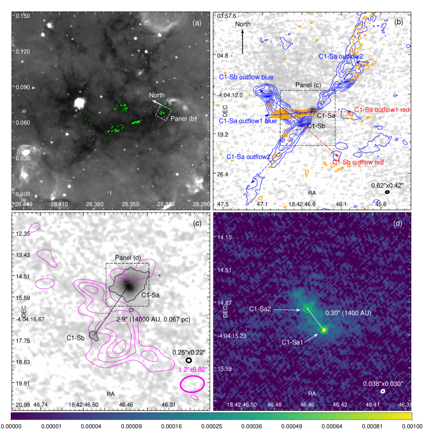
Figure 1: (a): Spitzer $8\mu$m image of the Dragon IRDC (in galactic coordinates). The green contours mark the 1.3 mm continuum dust emission from C3 (see §2) at SNR=5, 10, 15 (RMS_cont=80 $\mu$Jy beam^-1). (b): A zoom-in view of the C1-Sa and C1-Sb cores (with the C3 data, in equatorial coordinates, black ellipse beam). The grey scale map shows the 1.3 mm continuum emission from panel (a). The blue contours show the integrated intensity of ¹²CO(2-1) for C1-Sa outflow2 at SNR=9, 18, …, 72 (RMS_mom0=10 mJy beam^-1 km s^-1). The orange contours show the integrated intensity of SiO(5-4) at SNR=3, 7, …, 31 (RMS_mom0=6 mJy beam^-1 km s^-1). (c): A zoom-in view of C1-Sa and C1-Sb, showing the C2 1.3 mm continuum image with a factor of 2 higher resolution (in equatorial coordinates, black ellipse beam). The black contour shows the continuum at SNR=5. The magenta contours show the C4 ortho-H₂D⁺ line integrated intensity at SNR=2, 3, 4, 5 (RMS_mom0=10 mJy beam^-1 km s^-1, magenta ellipse beam). (d): The new C7 1.3 mm continuum image (C7Briggs0.5, in equatorial coordinates, white ellipse beam). The field-of-view shows the two kernels in C1-Sa, which we name C1-Sa1 and C1-Sa2, both showing a centrally-peaked circular morphology. The yellow circles show the kernel definition (see §3.1). The color bar is in Jy beam^-1.

Figure 1 shows the core fragmentation hierarchy. Panel (a) shows an overview of the Dragon IRDC which is the dark absorption feature in the Spitzer $8\mu$m image from the GLIMPSE survey (Benjamin et al., 2003; Churchwell et al., 2009). The green contours show the 1.3 mm continuum mosaic from the C3 data. The C1-Sa and C1-Sb cores are in the Tail of the Dragon (inside the white dashed square, see Kong, 2019). This region has the highest column density of the IRDC (Lim & Tan, 2014) and is dark at up to 100 $\mu$m (Ragan et al., 2012).

Panel (b) shows the zoom-in view of the Tail region. Here we show the continuum emission, along with the CO and SiO integrated intensities in blue and orange contours, respectively. The two lines trace molecular outflows from protostars. As will be shown in §3.2, there are three bipolar outflows in the Tail region. Two of them (C1-Sa outflow 1 and C1-Sb outflow) were studied in detail in T16 and K18 (also see Feng et al., 2016). The third one (C1-Sa outflow 2) is identified in this paper. The arrows mark the three bipolar outflows. Here, both lines are integrated between 74 and 80 km s^-1 to focus on C1-Sa outflow2. This velocity range encloses the system velocity of $\sim 78$ km s^-1 (Carey et al., 1998; Pillai et al., 2006, T16, K18).

Panel (c) shows the two continuum cores with a factor of 2 better resolution. Here, C1-Sa shows an elongated morphology in the NE to SW direction. C1-Sb still appears to be a single weak structure. At a distance of 4.8 kpc, the two cores have a projected separation of $\sim$0.067 pc (14,000 AU). As shown in panel (b), C1-Sb coincides with the C1-Sa outflow2. It is not clear if C1-Sb is impacted by the outflow. But the outflow from C1-Sb does not show any evidence of it being disrupted (T16, K18).

The magenta contours show the ortho-H₂D⁺ integrated intensity. The integration is between 78.8 and 80.0 km s^-1. There is clear detection of ortho-H₂D⁺. The majority of the emission is between C1-Sa and C1-Sb, with some emission around C1-Sa. The ortho-H₂D⁺ spatial distribution is consistent with the distribution of N₂D⁺(3-2) from K18 (see their figure 3) . H₂D⁺ is the first step of deuterium fractionation in cold starless cores (e.g., Pagani et al., 2013; Kong et al., 2015). With its descendant N₂D⁺, ortho-H₂D⁺ has been used to search for the youngest dense cores (e.g., Pillai et al., 2012; Miettinen, 2020; Sabatini et al., 2020; Redaelli et al., 2021). The presence of both ortho-H₂D⁺ and N₂D⁺ in the C1-S region strongly indicates that the cores are in the earliest evolutionary stage (K18).

Panel (d) shows the zoom-in view of the C1-Sa core with the high-resolution C7 data. The overall continuum emission follows the NE to SW elongation in panel (c). The core fragments into two centrally-peaked, circular structures (also see Figure 2(c)(d)) with several smaller and irregularly-shaped structures. Hereafter, the circular structures are defined as kernels, and we name the two kernels C1-Sa1 and C1-Sa2. They have a projected separation of $\sim$1400 AU. The new C7 data confirms that C1-Sa is indeed a binary in the making.

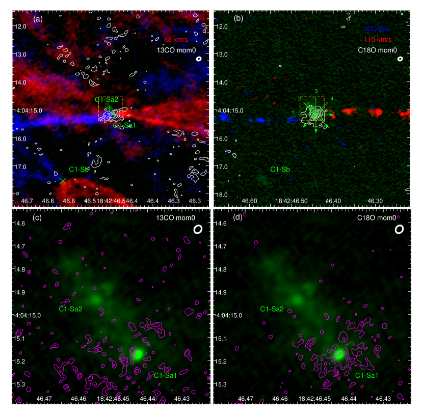
Figure 2: (a): RGB color map of C1-Sa and C1-Sa outflow1. The green color shows the 1.3 mm continuum (C7Briggs0.5), ranging from 0 to 1 mJy beam^-1 (SNR=40) in linear scale. The blue color shows the CO channel at 71 km s^-1. The red color shows the CO channel at 88 km s^-1. The white contours show the ¹³CO integrated intensity (C7Taper) at SNR=3, 5, 7. The orange dashed rectangle shows the field-of-view of panels (c)(d). (b): The continuum (green) is the same as panel (a) but in square-root scale. The blue color shows the SiO channel at 63 km s^-1. The red color shows the SiO channel at 115 km s^-1. The white contours show the C¹⁸O integrated intensity (C7Taper) at SNR=3, 5, … 13. The green arrows show positions of the cuts used for the position-velocity diagrams shown in Figure 4. Each cut is centered at C1-Sa1. (c): Comparison between 1.3 mm continuum (green, C7Briggs0.5) and ¹³CO integrated intensity (magenta contour, C7Briggs0.5). The contour levels are SNR=2, 3, 4. (d): Comparison between 1.3 mm continuum (green, C7Briggs0.5) and C¹⁸O integrated intensity (magenta contour, C7Briggs0.5). The contour levels are SNR=2, 3, 4. Integration ranges and RMS noises are presented in text in §3.3.

We carry out 2D Gaussian fitting to the kernels. The C1-Sa2 fitting is affected by its surrounding emission. So we simply adopt the centers from the fitting but define the kernels with circles. The yellow circles in Figure 1(d) show the kernel definition. For C1-Sa1 the circle is at 3$\sigma$ level of the Gaussian fitting. For C1-Sa2 the circle is smaller than the 3$\sigma$ level of the fitting but covers the circular kernel visually. The position error for C1-Sa1 fitting is 3% of a pixel (0.003″); for C1-Sa2 is 10% of a pixel. Table 2 summarizes the kernel definition. From now on, we assume a spherical geometry in 3D for the two kernels.

Table 2: Kernel Definition and Properties

Kernel	RA	DEC	$R$	$D$	$I_{\rm peak}$	$S_{\rm 1.3}$	$M$	$V_{\rm LSR}$	$\Delta V$
	J2000	J2000	arcsec	AU	mJy beam-1	mJy	M⊙	km s-1	km s-1
C1-Sa1	18:42:46.4429	-4:04:15.175	0.044	420	1.46(0.02)	3.4(0.6)	0.55(0.09)	78.59(0.06)	0.60(0.06)
C1-Sa2	18:42:46.4550	-4:04:14.939	0.044	420	0.54(0.02)	2.2(0.6)	1.8(0.5)	-	-

Note. — The kernel radii are not forced to be the same in the fitting.

3.2 C1-Sa Outflows

In Figure 1(b), there are two bipolar outflows that are visually associated with C1-Sa. The first (C1-Sa outflow1) was identified in T16 and K18. The second (C1-Sa outflow2) is a bit ambiguous as its two lobes show up in the same CO channel maps (T16). This is unlike most other symmetric outflows that typically show one lobe in blue-shifted channels and the other in red-shifted channels, or monopolar outflows (e.g., Fernández-López et al., 2013). However, the SiO(5-4) integrated intensity contours nicely overlap with the CO counterparts in panel (b), especially in the north-west end (the bifurcation feature). The morphological match between the two outflow tracers, which is seen in many other outflows in this IRDC (see Kong et al., 2019), strongly indicates that C1-Sa outflow2 is indeed a bipolar outflow. The axis of this outflow is probably parallel to the plane of the sky, which is why the two lobes always appear in same channels. Feng et al. (2016) saw the same NW to SE structure in SiO(2-1) at a lower resolution. They suspected that the bipolar SiO(2-1) emission belonged to a second outflow, consistent with our findings here. Visually, C1-Sa outflow2 clearly points toward C1-Sa, which is why this outflow is named after C1-Sa. However, C1-Sa outflow2 is not like C1-Sa outflow1 that connects to the C1-Sa core. There is a small gap between the outflow and the core.

Figure 2(a) shows the C1-Sa outflow1 in CO with the latest C7 data. The outflow is clearly launched from C1-Sa1, the brightest kernel of the two. The red lobe shows a nice fan-like morphology, while the blue lobe is more like a narrow jet. The C1-Sb bipolar outflow is also visible to the south-east. Notably, C1-Sb is relatively fuzzy in the high-resolution continuum data (see panel (b), for comparison see K18 Figure 1), suggesting that the core is not very centrally-peaked. However, it launches a bipolar outflow. But the outflow is not as collimated as those from C1-Sa.

Figure 2(b) shows C1-Sa outflow1 in SiO. Here we see multiple knots in the outflow, probably indicating accretion bursts in C1-Sa1 (see another example in Plunkett et al., 2015). A visual inspection of the larger area shows that there are at least 6 burst knots in each lobe of the outflow. The knots are approximately equally-spaced, with a typical projected separation $l_{\perp}$=1″, equivalent to 4800 AU or 0.023 pc in the plane of the sky. The line-of-sight velocity $v_{\parallel}$ for the blue knots is 15 km s^-1 and for the red is 37 km s^-1 (adopting a system velocity of 78 km s^-1), which implies more than a factor of two difference between the red and blue (also seen in T16). Assuming the same outflow velocity between the two lobes, the mismatch $v_{\parallel}$ indicates that the blue lobe has a larger $i$. Alternatively, the blue lobe is plunging into denser gas so that it is decelerated.

If we simply adopt a line-of-sight knot velocity of 30 km s^-1, the burst interval $\delta t=l_{\perp}/v_{\parallel}/tan(i)\approx 450$ yr, where the inclination angle relative to our line-of-sight $i$ is set at 60° to be consistent with T16. The very rough estimation suggests that the accretion bursts take place regularly on a timescale on the order of 500 yr.

3.3 Line Detection

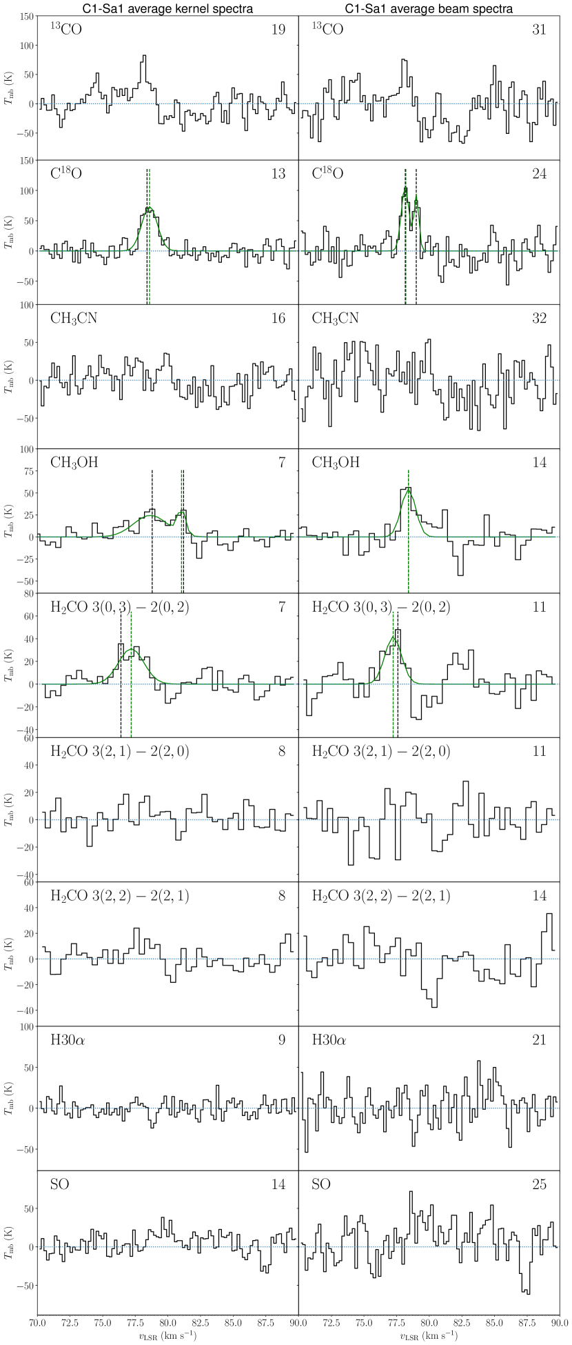
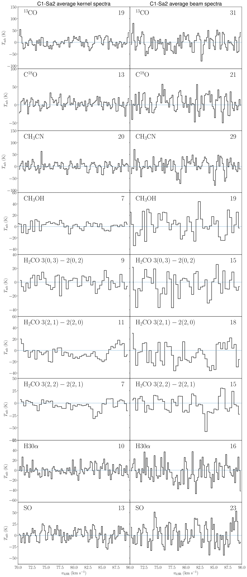
Figure 3: C1-Sa1 spectra (left) and C1-Sa2 spectra (right) from C7Briggs0.5. For each source, we show both average spectra within the kernel and the beam. If a local peak (black dashed vertical line) has at least 3 adjacent channels with SNR$\geq$2, it is identified as a component and fitted with a Gaussian (green curve). The line noise RMS_line in K is shown at the top-right. The black vertical dashed line indicates the line peak. The green vertical dashed line marks the Gaussian peak.

Figure 2(a)(b) show the integrated intensity contours of ¹³CO and C¹⁸O (C7Taper). The integration is over 77.3 km s^-1 to 80.0 km s^-1, with RMS_mom0 $\sim$2.2 mJy beam^-1 km s^-1. One can see that both molecular lines clearly show a centrally-peaked emission structure at C1-Sa1. In the ¹³CO contour map, there is a concave emission pattern around C1-Sa2. In C¹⁸O, C1-Sa2 is on the periphery of the contours. C1-Sa2 does not show a centrally-peaked molecular line emission.

In Figure 2(c)(d), we zoom in to show the detailed emission around the two kernels. Here we overlay the C7Briggs0.5 ¹³CO and C¹⁸O integrated intensity contours on top of the C7 continuum image. The integration is over 77.3 km s^-1 to 80.0 km s^-1, with RMS_mom0 $\sim$1.8 mJy beam^-1 km s^-1. Again, C1-Sa2 is neither detected in ¹³CO nor C¹⁸O, while C1-Sa1 shows clumpy detection in both lines. There is a void of C¹⁸O toward C1-Sa2, indicating that the NE part of the dust elongation is cold enough that the C¹⁸O is reduced from gas-phase due to freeze-out, which is consistent with the spatial distribution of ortho-H₂D⁺ (Figure 1(c)). C1-Sa2 is either starless or at a very early evolutionary stage with undetectable lines or outflows (see below).

Comparing C1-Sa1 and C1-Sa2, we argue that C1-Sa outflow2 could not have been launched by C1-Sa2. C1-Sa outflow2 is much more extended than C1-Sa outflow1 in the sky plane. If it was indeed from C1-Sa2, C1-Sa2 should at least show similar ¹³CO and C¹⁸O detection as C1-Sa1 because of heating of the environment by the protostar. One could argue that C1-Sa outflow2 from C1-Sa2 was significantly reduced for some reason a while ago. The gap between C1-Sa and one lobe from C1-Sa outflow2 is about 1″, corresponding to 4800 AU which takes 770 yr for a 30 km s^-1 outflowing gas to traverse. Given the length of the C1-Sa outflow2, the presumed C1-Sa2 protostellar accretion must have lasted around ten thousand years (one outflow lobe is about 20″, and assuming a velocity of 30 km s^-1, the timescale is 16000 yr). It is hard to imagine that C1-Sa2 had a protostar for about ten thousand years then significantly reduced accretion and resumed CO freeze-out within a thousand years (the timescale of the gap). In addition, we see no hint of outflowing gas connecting to C1-Sa2 (see §4.1). A more plausible scenario is that C1-Sa2 is still starless.

In Figure 3, we plot molecular line spectra for the two kernels. For each kernel, we show both a spectrum averaged over the size of the kernel and spectrum average over the size of the beam, centered at the kernel position. Note that the kernel size ($\sim$0.09″) is $\sim$3 times the beam size ($\sim$0.03″). We adopt an automated routine to find and fit Gaussian profiles in the spectra. Only those velocity components with at least 3 adjacent channels greater than twice the spectral noise are considered.

C1-Sa1 shows clear detection in C¹⁸O, CH₃OH 4(2)-3(1) E1 vt=0, and H₂CO 3(0,3)-2(0,2). The ¹³CO detection is marginal and not captured by the auto-fitting routine. A visual inspection of the channel maps shows that the C1-Sa outflow1 is detected in CH₃OH 4(2)-3(1) E1 vt=0, H₂CO 3(0,3)-2(0,2), H₂CO 3(2,1)-2(2,0), H₂CO 3(2,2)-2(2,1), SO, and SiO. So the detection of CH₃OH and H₂CO in the C1-Sa1 spectra is probably contaminated by the outflow. C1-Sa2 shows no clear detection in any of the lines, which is consistent with it being starless.

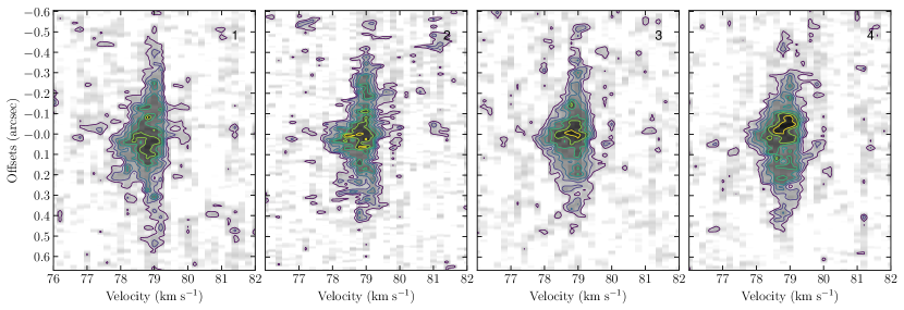
Figure 4: C¹⁸O(2-1) position-velocity diagrams across C1-Sa1 (using C7Briggs1). Each panel shows the diagram along the cut as denoted by the relevant arrow in Figure 2(b). The offset direction follows the arrow direction. C1-Sa1 is at zero offset. The color range is from 0 to 0.01 Jy beam^-1 (SNR=10). The color map is also shown in contours, with levels ranging from SNR=2 to SNR=10 at a step of SNR=1.

In C1-Sa1, the C¹⁸O kernel spectrum shows a Gaussian profile. The fitted line centroid velocity is $78.59\pm 0.06$ km s^-1, with a velocity dispersion of $0.60\pm 0.06$ km s^-1. However, the beam spectrum shows a double-peak feature with the red peak being weaker. Their separation is 0.87$\pm$0.06 km s^-1. The double-peak feature only appears at the kernel center. Figure 4 shows C¹⁸O position-velocity diagrams along four cuts through C1-Sa1 as shown in Figure 2(b). They all show a line-broadening near offset 0 (the location of the kernel), which is consistent with the spectra. Note, the line-broadening is most obvious at blue-shifted velocities but suppressed at red-shifted velocities in the position-velocity diagram. As will be shown in §3.4, the C¹⁸O line is optically thick. Therefore, the double-peak feature is probably due to self-absorption by the red-shifted colder gas on the near side. Gravitational infall at the kernel center can explain these spectral features (e.g., the blue profile in Evans, 1999). On the other hand, there is no clear velocity gradient across C1-Sa1 in any of the four position-velocity diagrams. They all show a main velocity component at $\sim$79 km s^-1. The lack of gradient indicates a lack of rotation across C1-Sa1 (to the accuracy of the velocity resolution of $\sim 0.2$ km s^-1) above the scale of $\sim$300 AU (C7Briggs1 beam size of 0.06″).

3.4 Physical Properties

In C1-Sa, K18 adopted a fiducial dust temperature of 20 K for the entire core and derived a mass of 33.5 M_⊙. Hereafter, we adopt their fiducial temperature and mass for C1-Sa. The corresponding column density is 22000 M_⊙ pc^-2 ($\Sigma=4.7$ g cm^-2 or $N_{H}=2.0\times 10^{24}$ cm^-2). For the moderately coagulated thin ice mantle model $\kappa_{\nu}=0.899$ cm² g^-1 at 1.3 mm (Ossenkopf & Henning, 1994), the core optical depth $\tau_{1.3}=\Sigma\kappa_{\nu}/R_{\rm gd}=0.028$ (assuming a gas-to-dust mass ratio $R_{\rm gd}=141$, Draine, 2011), i.e., still optically thin. The particle number density is $n=1.3\times 10^{7}$ cm^-3 (assuming a mean molecular weight per free particle of 2.37, K18). At such high density, the gas temperature is expected to be the same as the dust temperature (20 K), and thus the sound speed, $c_{s}$, should be about 0.3 km s^-1. With these properties, the Jeans length is about $0.005$ pc (1100 AU), which is comparable to the projected separation between C1-Sa1 and C1-Sa2 (§3.1). Unless the elongated structure of C1-Sa is significantly inclined with respect to the plane of the sky, in which case the 3D separation is much larger than the projected separation, the distance between the kernels suggests a thermal fragmentation scenario for the binary formation. At present no observations clearly constrain the inclination.

We fit the C1-Sa core C¹⁸O(2-1) spectra from the C2 data (K18) and C3 data (K21) at the scale of 1.8″(averaged within a diameter of 1.8″, or 0.042 pc, which was the diameter of C1-Sa in the K18 definition). Both fits give a velocity dispersion $\sigma_{18}=0.30\pm 0.02$ km s^-1 which is approximately the sound speed $\sigma_{18}\approx c_{s}$. This means the non-thermal motion is sub/transonic as we subtract the thermal component from the C¹⁸O line dispersion. If the non-thermal component is tracing turbulence, then the data shows that turbulence becomes less dominant at the scale of C1-Sa, which is consistent with the thermal fragmentation argument above.

Interestingly, if we fit the spectra at a scale of 1.0″ (average spectrum over the size of the scale), the C2 data gives $\sigma_{18}=0.33\pm 0.01$ km s^-1 while the C3 data gives $\sigma_{18}=0.35\pm 0.03$ km s^-1. If we fit the spectra at a scale of 0.5″, the C2 data gives $\sigma_{18}=0.34\pm 0.01$ km s^-1 while the C3 data gives $\sigma_{18}=0.36\pm 0.03$ km s^-1. The fact that the line dispersion is constant/increases at smaller scales (from 1.8″ to 0.5″) indicates that it is not tracing turbulence decay from larger scales, consistent with the above result that turbulence is less important. At an even smaller scale (the kernel scale of C1-Sa1 0.088″), the line dispersion becomes $0.60\pm 0.06$ km s^-1 (§3.3). This increasing linewidth could trace the gravitational collapse that accelerates closer to C1-Sa1 (e.g., see Ballesteros-Paredes et al., 2011). Or, it is due to the line-broadening from high optical depth (see below). Another possibility is that it is tracing the rotation inside C1-Sa1 (§4.1).

We compute the kernel mass with the following equation

$$M=\frac{S_{\nu}D^{2}R_{\rm gd}}{B_{\nu}(T_{\rm dust})\kappa_{\nu}},$$ (1)

where $S_{\nu}$ is the continuum flux density, $D$ is the distance (4.8 kpc), $R_{\rm gd}$ is the gas-to-dust mass ratio (141, Draine, 2011), $B_{\nu}(T_{\rm dust})$ is the Planck function at the dust temperature, and $\kappa_{\nu}$ is the dust opacity. We adopt $\kappa_{\nu}=0.899$ cm² g^-1 for the moderately coagulated thin ice mantle model from Ossenkopf & Henning (1994). If we again adopt a dust temperature of 20 K, the mass for C1-Sa1 is 2.6 M_⊙ (but see below), and for C1-Sa2 is 1.6 M_⊙.

The above C1-Sa1 mass at 20 K corresponds to a volume density of $n_{\rm H_{2}}=8.2\times 10^{9}$ cm^-3, and a column density of $N_{\rm H_{2}}=3.5\times 10^{25}$ cm^-2. Assuming no CO freeze-out in C1-Sa1, the corresponding C¹⁸O column density is $N_{\rm C^{18}O}=1.9\times 10^{19}$ cm^-2, assuming the ISM abundance [C¹⁸O/H₂]=$5.4\times 10^{-7}$ (Wilson & Rood, 1994; Gerin et al., 2015). The C1-Sa1 C¹⁸O kernel spectrum had a line dispersion of 0.60 km s^-1, corresponding to a linewidth of 1.4 km s^-1. Putting these numbers into the RADEX code (van der Tak et al., 2007), assuming a gas kinetic temperature of 20 K, the C¹⁸O line optical depth $\tau_{18}$ reaches 1500.

However, under such conditions, the line intensity is only 15 K based on RADEX, much smaller than what we observe (see Figure 3). To crank up the line intensity, one has to increase the kinetic temperature which is the only uncertain variable in the above calculation. In short, if C1-Sa1 has a kinetic temperature of 75 K, the line intensity estimated by RADEX of 70 K would match the C1-Sa1 kernel spectrum in Figure 3, and the corresponding mass would be 0.55 M_⊙ (still using Eq. (1) but $T_{\rm dust}=75$ K). Note, the Jeans mass in C1-Sa (the enclosing core) is 0.087 M_⊙, which is significantly smaller than the kernel mass. Perhaps magnetic fields provide additional support. For instance, Liu et al. (2020) showed an ordered magnetic field which is well aligned with the elongation of C1-Sa (NE-SW). Alternatively, they probably have accreted material from C1-Sa, i.e., their larger mass is not the mass that directly results from the fragmentation.

The C1-Sa1 mass is a factor of 3 smaller than C1-Sa2. The difference can be explained by the protostellar accretion in C1-Sa1. For instance, if the two kernels had a similar initial mass, then the missing mass in C1-Sa1 could have been accreted by the embedded protostar. With the new estimation for C1-Sa1 (0.55 M_⊙), the volume density becomes $n_{\rm H_{2}}=1.8\times 10^{9}$ cm^-3, and the column density becomes $N_{\rm H_{2}}=7.4\times 10^{24}$ cm^-2. Assuming the same ISM abundance [C¹⁸O/H₂]=$5.4\times 10^{-7}$, the C¹⁸O column density becomes $N_{\rm C^{18}O}=4.0\times 10^{18}$ cm^-2. The updated RADEX calculation gives an optical depth of 35, i.e., the C¹⁸O line is optically thick.

For C1-Sa2, using the mass calculation at 20 K, the volume density is $n_{\rm H_{2}}=5.3\times 10^{9}$ cm^-3, and the column density is $N_{\rm H_{2}}=2.2\times 10^{25}$ cm^-2. If there is no CO freeze-out in C1-Sa2, the corresponding C¹⁸O column density is $N_{\rm C^{18}O}=1.2\times 10^{19}$ cm^-2. Assuming a linewidth of $\sim$1.4 km s^-1, the C¹⁸O(2-1) line intensity based on RADEX is 15 K, which is the same as C1-Sa1 at 20 K because the line emission is saturated with an optical depth of 970. The 15 K line intensity is non-detectable in the kernel spectrum in Figure 3 which has an RMS_line noise of 12 K. Only if we increase the kernel temperature to 40 K would the C¹⁸O(2-1) line intensity be high enough to be detectable with SNR of 3, albeit still being optically thick. Therefore, the non-detection of C¹⁸O in C1-Sa2 sets an upper limit of the kernel temperature to 40 K.

The surface density of C1-Sa1 is $\Sigma=34$ g cm^-2. The corresponding optical depth is 0.20, i.e., optically thin. Meanwhile, we estimate the surface density for C1-Sa2 to be $\Sigma=100$ g cm^-2. The optical depth is 0.62. The continuum flux for C1-Sa1 is 3.4 mJy, for C1-Sa2 is 2.2 mJy. The corresponding Planck brightness temperature (the equivalent temperature with which the Planck function gives the flux) for C1-Sa1 is 15 K, for C1-Sa2 is 11 K. Since the dust continuum is optically thin, the above brightness temperatures are lower limits of the kernel temperature.

4 Discussion

4.1 C1-Sa Outflow2 Origin from C1-Sa1

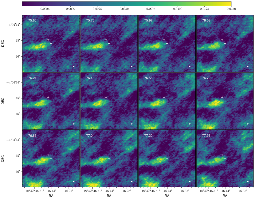
Figure 5: Zoom-in CO channel maps at C1-Sa1 outflow2 velocities (C7Natural). The channel velocity is labeled at the top-left in km s^-1. The linear-scale color range is between SNR=-3 and SNR=10 (RMS_line=1.5 mJy beam^-1). The two kernels are marked as white crosses (C1-Sa1 at the map center). C1-Sa outflow1 is the bright structure in the middle pointing eastward. Only its blue lobe is visible (see Figure 2). C1-Sa outflow2 is the bright structure from lower-left to upper-right.

In §3.2, we have shown that C1-Sa launches two outflows, include C1-Sa outflow2. In §3.3, we have argued that C1-Sa outflow2 is not from C1-Sa2. Therefore, C1-Sa1 is the only candidate for the launching source of C1-Sa outflow2. Figure 5 shows the spatial relation between the two kernels and the outflows. Here, we show CO channel maps from C7Natural, focusing on channels in which the C1-Sa outflow2 is present. Again, C1-Sa outflow1 is clearly from C1-Sa1. Meanwhile, C1-Sa outflow2, though not clearly contacting to the two kernels, appears to be spatially closer to C1-Sa1. There is some weak emission feature (SNR$\geq$2) extending from C1-Sa outflow2 and pointing toward C1-Sa1. Here we argue that C1-Sa outflow2 originates from the C1-Sa1 kernel.

Two scenarios could explain the origin of C1-Sa outflow2. In the first scenario, there is only one protostar in C1-Sa1. It initially launched C1-Sa outflow2. About 770 yr ago (the gap between C1-Sa outflow2 and C1-Sa1, see §3.3), the accretion was significantly reduced and a new outflow (C1-Sa outflow1) was launched at a different direction. In this scenario, the change in outflow direction could have been caused by a change in direction of the accretion disk angular momentum vector. However, based on the outflow bursts, the age of C1-Sa outflow1 should be at least 6 times the burst interval (6$\times$450 yr=2.7 kyr, see §3.2). So C1-Sa outflow1 already existed before C1-Sa outflow2 weakened.

A more plausible scenario is that C1-Sa1 hosts a tight binary that is not resolved by the ALMA synthesized beam of 140 AU. One launched C1-Sa outflow2 first and the other launched C1-Sa outflow1 later. Both outflows co-existed for a while and one of them significantly weakened 770 yr ago. The double-peak C¹⁸O line (optically thick) could show the overall infall in C1-Sa1 (the “blue profile”, Evans, 1999), or the radial velocity of the tight binary (each peak tracing a member), or the rotational velocity of an edge-on disk (a circumbinary disk or the circumstellar disks) that is not resolved.

4.2 Further Fragmentation

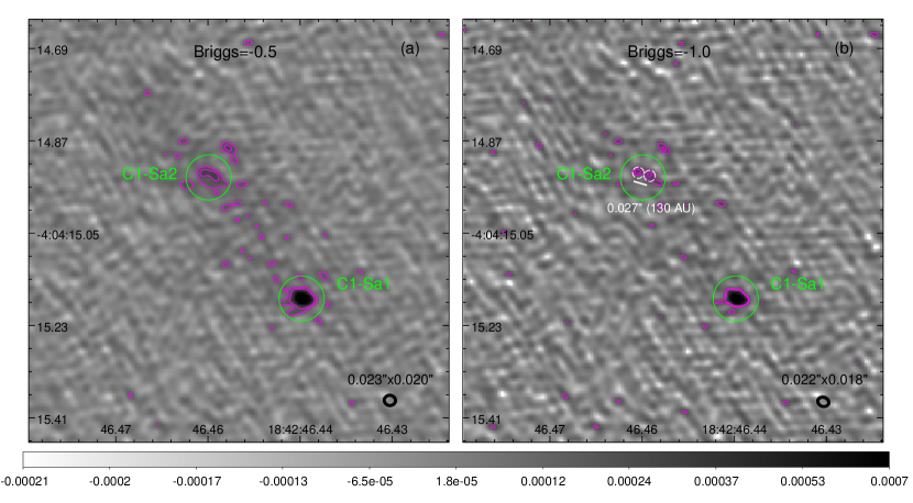
Figure 6: (a): C7Briggs-0.5 1.3 mm continuum image. The linear color scale is in unit of Jy beam^-1. The magenta contours show emission at SNR=3,5 with RMS_cont=50$\mu$Jy beam^-1. (b): Same field of view and same color scale as panel (a), but with C7Briggs-1 1.3 mm continuum. The magenta contours show emission at SNR=3,4 with RMS_cont=70$\mu$Jy beam^-1. The white dashed circles show the definitions of the sub-kernels of the potential pre-binary, both having a diameter of 0.022″, or 100 AU. Their separation (0.027″ or 130 AU) is marked by the white segment.

In Figure 6, we show the C7 1.3 mm continuum image with an even higher resolution than the previous images. Panel (a) shows the C7Briggs-0.5 image with a synthesized beam size of about 0.022″. Panel (b) shows the C7Briggs-1 image with a beam size of approximately 0.02″ (96 AU). With the higher resolution, we see C1-Sa1 starts to show irregular shapes at its periphery, which seems to support the tight binary scenario because a single protostar should maintain a form of symmetry in its morphology. Still, no clear signature of disks is obvious in the image, constraining the disk sizes to be smaller than 96 AU. Higher angular resolution observations are needed to confirm the potential tight binary.

In Figure 6, C1-Sa2 splits into two sub-kernels, or a potential pre-binary, both detected at SNR=4. Their projected separation is $\sim$130 AU. In panel (b), we simply define the sub-kernels with two circles that cover the continuum emission (white dashed circles). They both have a flux density of 290$\pm 70\mu$Jy (due to rounding), translating to a mass of $\sim 0.17\pm 0.04$ M_⊙ assuming a 20 K dust temperature (Eq. (1)). The free particle number density of C1-Sa2 is $n=6.1\times 10^{9}$ cm^-3. The corresponding Jeans scale is 57 AU, and the corresponding Jeans mass is 0.0040 M_⊙. In §3.4, we set a temperature upper limit of 40 K. Since C1-Sa2 has no outflow detection and there is ortho-H₂D⁺ (Figure 1) and N₂D⁺ (K18) in the vicinity, its temperature cannot be much higher than 20 K based on deuterium chemistry (e.g., Kong et al., 2015).

Note in C7Briggs0.5 (Figure 2(b)), C1-Sb is not as centrally-concentrated as C1-Sa2 and has a factor of $\gtrsim$3 weaker 1.3 mm emission than C1-Sa2, yet its outflow is clearly detected. So either C1-Sa2 has no outflow or its outflow is still too weak/small to be detected, putting it at a very early stage with likely a lower temperature. The blob to the north-west (§3.1) remains singular. Altogether, the whole C1-Sa core is potentially developing a quintuple system within a scale of $\sim$1000 AU. However, we caution that the fragmentation of C1-Sa2 is to be further confirmed with higher sensitivity observations.

4.3 Binary Star Formation

The massive ($\sim 30$ M_⊙), 100 $\mu$m-dark core C1-Sa shows a hierarchical structure. The core itself harbors a binary system at the two ends of an elongated structure. Each member of the binary shows signs of further fragmentation.

If the misaligned outflows in C1-Sa1 indeed indicate a tight binary with misaligned disks, then the misalignment argues against disk fragmentation. On the other hand, turbulence is sub/transonic at the sub-core scale based on the C¹⁸O line fitting. So the origin of the hypothesized binary is unclear. Possibly, the tight binary simply forms via thermal fragmentation, just like C1-Sa1 and C1-Sa2 in C1-Sa. Then, it remains to be seen how the disk angular momenta are determined at $\lesssim$100 AU scale.

On the other hand, we can assume that the source which used to drive C1-Sa outflow2 was born first, and the other source that drives C1-Sa outflow1 formed later. We assume this order simply because C1-Sa outflow2 is much longer (in size) than C1-Sa outflow1 (unless C1-Sa outflow1 is oriented close to the line-of-sight). Based on the rough estimation in §3.3, the accretion associated with C1-Sa outflow2 was drastically reduced about 770 yr ago. But about 3 kyr (§4.1) ago, the accretion associated with C1-Sa outflow1 began (§3.2). This time mismatch argues against the scenario in which a protostellar outflow changes orientation due to turbulent accretion (e.g., Offner et al., 2016). So the formation history of the tight binary could be described as the following: a protostar formed in C1-Sa1 first and launched C1-Sa outflow2; then another protostar formed and launched C1-Sa outflow1; both protostars were accreting for some time before the first protostar, which was driving C1-Sa outflow2, switched to a much weaker accretion.

The fragmentation of C1-Sa2 provides a valuable example of the primordial state of binary formation (if further confirmed with a better sensitivity). Although currently we have no kinematic information for C1-Sa2, the fact that it appears as a spherically symmetric structure (Figure 1(d), Figure 2(c)(d)) similar to C1-Sa1 indicates that it is a bound entity. So the pre-binary in C1-Sa2 is also likely bound. The boundness of the final binary system depends on the accretion. The fragmentation length ($\sim 130$ AU) and mass ($\sim$0.17 M_⊙) are larger than the Jeans scale ($\sim 57$ AU) and Jeans mass ($\sim$0.004 M_⊙) of C1-Sa2. So perhaps further fragmentation will happen. Note, at such high density of C1-Sa2, the free-fall timescale is just $\sim$550 yr. Once the protostar lights up, the temperature increase should suppress fragmentation (e.g., Krumholz, 2006).

4.4 Comparison with other observations and theories

Compared with other protobinary observations, C1-Sa is in a very different environment. It is in the highly extincted, quiescent region of the massive Dragon IRDC (the southern Dragon Tail, Lim et al., 2016; Kong, 2019). There is no nearby massive star/protostar within 5 pc. This condition is quite different from, e.g., IRAS 16547-4247 (Tanaka et al., 2020), or G11.92-0.61 MM2 (Cyganowski et al., 2022), both having in-situ/nearby massive protostar. Therefore, C1-Sa is one of the first-generation stars in the IRDC. Its environment has not been impacted by fierce feedback from massive stars. T16 estimated the mass outflow rate and the momentum injection rate for C1-Sa outflow1, and concluded that C1-Sa is a good candidate for early-stage massive protostar. Given now we show that C1-Sa is a binary system, it provides an excellent example of the early, pristine stage of massive binary formation.

If the C1-Sa fragmentation (which gives C1-Sa1 and C1-Sa2) is via disk fragmentation, we should see disk/spiral structures in the continuum map (e.g., Krumholz et al., 2009; Oliva & Kuiper, 2020; Mignon-Risse et al., 2021). At 20 K, the column density detection limit (again using dust continuum) is $\sim 2.0$ g cm^-2 or $N_{\rm H_{2}}=4.4\times 10^{23}$ cm^-2, which should allow us to see spiral structures similar to those in the above simulations. If we assume a higher temperature as in C1-Sa1, the detection limit becomes even lower. One could argue that C1-Sa is edge-on so that the elongation in C1-Sa is the disk plane. However, the C¹⁸O position-velocity diagrams (§3.3) show no obvious velocity gradients across C1-Sa. Possibly, the structures are rather smooth and not captured by the interferometric images. The C1-Sa1 and C1-Sa2 separation matches well with that in Krumholz et al. (2009) though.

If the C1-Sa fragmentation is simply a thermal fragmentation, it is still crucial to know what exactly the elongated structure is in C1-Sa. It shows little velocity gradient, as illustrated in the C¹⁸O position-velocity diagrams (§3.3). It aligns well with magnetic fields (Liu et al., 2020). The field appears to be quite uniform (to be confirmed with more observations), suggestive of a sub-Alfvénic condition, which disfavors binary formation (e.g., Rosen & Krumholz, 2020; Mignon-Risse et al., 2021). If so, the field needs to dissipate with certain non-ideal MHD effects. The elongated structure shows multiple small continuum peaks that are either interferometric effects or local fragments.

The hypothesized binary in C1-Sa1 has a separation below 96 AU. Their outflows appear to be quite straight and collimated, showing no clear sign of precession, suggesting that the relevant accretion has been quite stable. The binary members probably have formed in-situ and their separation reflects their fragmentation scale. Such a small scale favors the disk fragmentation scenario rather than turbulent fragmentation (Offner et al., 2022). However, their misaligned outflows argue against disk fragmentation. Higher angular resolution observations are necessary to show the sub-structures of C1-Sa1.

A bolder hypothesis is that C1-Sa1 evolved just like C1-Sa2, but earlier, since the two kernels are born in the same environment. So the structure of C1-Sa2 gives us clues of what happened in C1-Sa1. The two fragments in C1-Sa2 roughly align on a filamentary structure, although C1-Sa2 itself is approximately spherical at a larger scale. Once one of the two fragments in C1-Sa2 forms a protostar, which it may already be doing, the entire C1-Sa2 kernel is lit up. The two fragments may possess gas with different angular momentum and thus launch misaligned outflows.

5 Conclusion

In this paper, we have reported ALMA Cycle 7 high-resolution observations toward the massive protostellar core C1-Sa, located at the highest extinction region in the Tail of the Dragon IRDC (aka G28.34+0.06 or G28.37+0.07). At the resolution scale of 140 AU, C1-Sa fragments into two centrally-peaked kernels (C1-Sa1 and C1-Sa2), each having a diameter of $\sim$420 AU. Their projected separation is $\sim$1400 AU, comparable to the Jeans scale of 1100 AU, consistent with a thermal fragmentation origin, unless the young binary is highly inclined to the line-of-sight. The thermal fragmentation is also consistent with the fact that C1-Sa has a sub/transonic non-thermal velocity dispersion based on the C¹⁸O modeling. We suspect the non-thermal motion (partially) comes from gravitational collapse because the C¹⁸O linewidth increases toward smaller scales.

There are two bipolar outflows coming out of C1-Sa, which we name C1-Sa outflow1 and C1-Sa outflow2. C1-Sa outflow1 was previously identified in T16 and K18 while C1-Sa outflow2 is only confirmed in this work with CO and SiO probably because C1-Sa outflow2 is parallel to the plane-of-the-sky. A detailed inspection suggests that both outflows are launched by C1-Sa1, the southern protostellar kernel in C1-Sa. C1-Sa2 is likely starless, which is consistent with the presence of N₂D⁺ and ortho-H₂D⁺ in its vicinity. There is a gap between C1-Sa outflow2 and C1-Sa1, indicating that the outflow was significantly reduced about 770 yr ago. C1-Sa outflow1 shows at least 6 bursty shocks, with interval between shocks of order 500 yr. We argue that C1-Sa1 has a tight binary, with each member launching a bipolar outflow and so presumably having its own accretion disk. Based on the large angle between C1-Sa outflow1 and C1-Sa outflow2, we argue that the two disks are misaligned.

C1-Sa1 is clearly detected in C¹⁸O(2-1) while C1-Sa2 has no obvious line detection. The latter is consistent with C1-Sa2 being starless. Based on RADEX modeling, the C¹⁸O line in C1-Sa1 is optically thick. So the double-peak feature in the beam spectrum and the lack of red-shifted emission in the position-velocity diagrams are likely due to self-absorption from the nearside cold infalling gas at the center of the kernel. The excitation temperature for the C¹⁸O line is about 75 K, which is also likely the gas and dust temperature in C1-Sa1 at the density of $n_{\rm H_{2}}=1.8\times 10^{9}$ cm^-3. The mass of C1-Sa1 is thus 0.55 M_⊙, a factor of 3 smaller than the presumably starless C1-Sa2 kernel, which we attribute to the protostellar accretion in C1-Sa1.

At the extreme resolution of the ALMA data (96 AU), C1-Sa2 further fragments into two sub-kernels with equal masses of 0.17 M_⊙, which requires further confirmation with higher sensitivities. The two fragments have a separation of $\sim$130 AU which is more than twice the C1-Sa2 Jeans scale at 20 K. At a density of $\sim 6.1\times 10^{9}$ cm^-3, C1-Sa2 has a free-fall timescale of just $\sim 550$ yr. A protostar could form before further fragmentation takes place. C1-Sa2 provides a good example of the initial condition for binary star formation. Meanwhile, C1-Sa1 shows deviation from the circular shape, hinting that it could further fragment, consistent with our speculation of the existence of a tight binary in this kernel. However, the hypothesized binary is not resolved at 96 AU.

The binary system is one of the earliest-stage forming binaries observed so far, which can potentially become massive. Its birth environment is a 100 $\mu$m-dark, potentially strongly magnetized massive core that is well-shielded and relatively quiescent (not impacted by nearby massive stars). The high surface density of this IRDC also creates a high pressure environment for the deeply embedded binary system. Therefore, the C1-Sa binary system gives us the opportunity to study (massive) binary formation in a very special environment. More similar studies will show how binary formation in such environments in IRDCs differs from binaries in other clouds. To our knowledge, the C1-Sa binary system is also the most distant forming binary observed thus far, reaching $\sim$5 kpc toward the near end of the Galactic Bar. Our study of the C1-Sa binary demonstrates that with ALMA, forming binaries can be detected and studied at these distances, significantly enlarging the parameter/volume space in which binary formation can be identified and studied, including a great number of IRDCs.

Appendix A Distance to the Dragon IRDC

The kinematic distance to the Dragon Nebula is $\sim$4.8 kpc (Carey et al., 1998). The cloud resides in the first Galactic quadrant at l$\sim$28 degrees where the radial velocity will yield a near and a far distance solution for kinematic distance measurements. Since the cloud is seen in absorption in the infrared against the diffuse emission of the galactic plane, a near distance has been widely adopted. HI self absorption (HISA) analysis towards this cloud shows a pronounced absorption feature at the systemic velocity (Anderson et al., 2010). This adds further confidence to the choice of the near distance. Depending on the model for the galactic rotation curve (e.g., Clemens, 1985; Reid et al., 2009), a distance between 4.5 and 5.0 kpc has been reported in the literature (Carey et al., 1998; Simon et al., 2006; Ragan et al., 2012).

Since the previous IRDC distance estimates, the galactic rotation curve (Reid et al., 2014) along with the revised solar motion parameters (Reid et al., 2019) have been updated. We have therefore used the online BeSSeL parallax based Distance Calculator that combines kinematic distance information with displacement from the galactic plane and proximity to individual parallax sources from the BeSSeL parallax survey (Reid et al., 2019) to generate a more complete distance probability density function for the cloud’s distance assignment. The systemic velocity of the cloud based on published H₂CO and NH₃ measurements is $\sim$78 km s^-1 (Carey et al., 1998; Pillai et al., 2006). The estimate of the cloud distance we obtain using this procedure is $4.34\pm 0.30$ kpc. Taking all the above information into consideration, we adopt 4.8 kpc as the fiducial distance to the IRDC to be consistent with previous literature.

Appendix B ortho-H₂D⁺ channel map

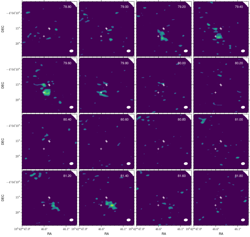
Figure 7: ortho-H₂D⁺ channel maps with detection. The channel velocity is labeled at the top-right in km s^-1. The two kernels are marked as white crosses (C1-Sa1 at the map center). C1-Sb core is also marked (to the south-east from C1-Sa1). Only emission at SNR$\geq$2 is shown.

Figure 7 shows the ortho-H₂D⁺ channel maps from the C4 data. The velocity range encompasses the detected ortho-H₂D⁺ emission, which overlaps with the N₂D⁺(3-2) emission detected in K18. From 79.2 km s^-1 to 79.8 km s^-1, the ortho-H₂D⁺ emission lies to the southeast of the two kernels, with the peak emission in the 79.6 km s^-1 channel. The location of the peak emission coincides with the N₂D⁺ core C1-S in K18. The high level of deuteration indicates that C1-S is at an early stage. One possibility is that C1-Sa, C1-Sb, and C1-S once belonged to a larger N₂D⁺ core (Tan et al., 2013). Once C1-Sa and C1-Sb became protostellar, their level of deuteration decreased, leaving over the C1-S core which can develop into another protostellar system (K18).

At 81.4 km s^-1, there is another peak emission of ortho-H₂D⁺ to the south-west of C1-Sa, which was never noticed before. Perhaps it will develop into another core/protostar. Currently, it only has detection within 0.4 km s^-1 (two channels). The channel velocity coincides with the C1-N core from Tan et al. (2013), which has a peak N₂D⁺ emission at $\sim$81.2 km s^-1. The tentative detection at the top-left corner in channel 81.2 km s^-1 in Figure 7 spatially coincides with C1-N, which is at the highest surface density region in Dragon Tail.

References

- Anderson et al. (2010) Anderson, L. D., Snowden, S. L., & Bania, T. M. 2010, ApJ, 721, 1319, doi: 10.1088/0004-637X/721/2/1319
- Astropy Collaboration et al. (2013) Astropy Collaboration, Robitaille, T. P., Tollerud, E. J., et al. 2013, A&A, 558, A33, doi: 10.1051/0004-6361/201322068
- Ballesteros-Paredes et al. (2011) Ballesteros-Paredes, J., Hartmann, L. W., Vázquez-Semadeni, E., Heitsch, F., & Zamora-Avilés, M. A. 2011, MNRAS, 411, 65, doi: 10.1111/j.1365-2966.2010.17657.x
- Beltrán et al. (2016) Beltrán, M. T., Cesaroni, R., Moscadelli, L., et al. 2016, A&A, 593, A49, doi: 10.1051/0004-6361/201628588
- Benjamin et al. (2003) Benjamin, R. A., Churchwell, E., Babler, B. L., et al. 2003, Publications of the Astronomical Society of the Pacific, 115, 953, doi: 10.1086/376696
- Bergin & Tafalla (2007) Bergin, E. A., & Tafalla, M. 2007, ARA&A, 45, 339, doi: 10.1146/annurev.astro.45.071206.100404
- Carey et al. (1998) Carey, S. J., Clark, F. O., Egan, M. P., et al. 1998, ApJ, 508, 721, doi: 10.1086/306438
- CASA Team et al. (2022) CASA Team, Bean, B., Bhatnagar, S., et al. 2022, PASP, 134, 114501, doi: 10.1088/1538-3873/ac9642
- Chini et al. (2012) Chini, R., Hoffmeister, V. H., Nasseri, A., Stahl, O., & Zinnecker, H. 2012, MNRAS, 424, 1925, doi: 10.1111/j.1365-2966.2012.21317.x
- Churchwell et al. (2009) Churchwell, E., Babler, B. L., Meade, M. R., et al. 2009, Publications of the Astronomical Society of the Pacific, 121, 213, doi: 10.1086/597811
- Clemens (1985) Clemens, D. P. 1985, ApJ, 295, 422, doi: 10.1086/163386
- Cyganowski et al. (2022) Cyganowski, C. J., Ilee, J. D., Brogan, C. L., et al. 2022, ApJ, 931, L31, doi: 10.3847/2041-8213/ac69ca10.48550/arXiv.2204.09163
- Draine (2011) Draine, B. T. 2011, Physics of the Interstellar and Intergalactic Medium, Princeton Series in Astrophysics (Princeton University Press)
- Duchêne & Kraus (2013) Duchêne, G., & Kraus, A. 2013, ARA&A, 51, 269, doi: 10.1146/annurev-astro-081710-102602
- Evans (1999) Evans, Neal J., I. 1999, ARA&A, 37, 311, doi: 10.1146/annurev.astro.37.1.311
- Feng et al. (2016) Feng, S., Beuther, H., Zhang, Q., et al. 2016, ApJ, 828, 100, doi: 10.3847/0004-637X/828/2/100
- Fernández-López et al. (2013) Fernández-López, M., Girart, J. M., Curiel, S., et al. 2013, ApJ, 778, 72, doi: 10.1088/0004-637X/778/1/72
- Gerin et al. (2015) Gerin, M., Ruaud, M., Goicoechea, J. R., et al. 2015, A&A, 573, A30, doi: 10.1051/0004-6361/201424349
- Gravity Collaboration et al. (2018) Gravity Collaboration, Karl, M., Pfuhl, O., et al. 2018, A&A, 620, A116, doi: 10.1051/0004-6361/201833575
- Hunter (2007) Hunter, J. D. 2007, Computing in Science and Engineering, 9, 90, doi: 10.1109/MCSE.2007.55
- Jones et al. (2001–) Jones, E., Oliphant, T., Peterson, P., et al. 2001–, SciPy: Open source scientific tools for Python. http://www.scipy.org/
- Joye & Mandel (2003) Joye, W. A., & Mandel, E. 2003, in Astronomical Society of the Pacific Conference Series, Vol. 295, Astronomical Data Analysis Software and Systems XII, ed. H. E. Payne, R. I. Jedrzejewski, & R. N. Hook, 489
- Kong (2019) Kong, S. 2019, ApJ, 873, 31, doi: 10.3847/1538-4357/aaffd5
- Kong et al. (2019) Kong, S., Arce, H. G., Maureira, M. J., et al. 2019, ApJ, 874, 104, doi: 10.3847/1538-4357/ab07b9
- Kong et al. (2021) Kong, S., Arce, H. G., Shirley, Y., & Glasgow, C. 2021, ApJ, 912, 156, doi: 10.3847/1538-4357/abefe7
- Kong et al. (2015) Kong, S., Caselli, P., Tan, J. C., Wakelam, V., & Sipilä, O. 2015, ApJ, 804, 98, doi: 10.1088/0004-637X/804/2/98
- Kong et al. (2018) Kong, S., Tan, J. C., Caselli, P., et al. 2018, ApJ, 867, 94, doi: 10.3847/1538-4357/aae1b2
- Krumholz (2006) Krumholz, M. R. 2006, ApJ, 641, L45, doi: 10.1086/503771
- Krumholz et al. (2009) Krumholz, M. R., Klein, R. I., McKee, C. F., Offner, S. S. R., & Cunningham, A. J. 2009, Science, 323, 754, doi: 10.1126/science.1165857
- Lim & Tan (2014) Lim, W., & Tan, J. C. 2014, ApJ, 780, L29, doi: 10.1088/2041-8205/780/2/L29
- Lim et al. (2016) Lim, W., Tan, J. C., Kainulainen, J., Ma, B., & Butler, M. J. 2016, ApJ, 829, L19, doi: 10.3847/2041-8205/829/1/L19
- Liu et al. (2020) Liu, J., Zhang, Q., Qiu, K., et al. 2020, ApJ, 895, 142, doi: 10.3847/1538-4357/ab9087
- Miettinen (2020) Miettinen, O. 2020, A&A, 634, A115, doi: 10.1051/0004-6361/201936730
- Mignon-Risse et al. (2021) Mignon-Risse, R., González, M., Commerçon, B., & Rosdahl, J. 2021, A&A, 652, A69, doi: 10.1051/0004-6361/202140617
- Moe & Di Stefano (2017) Moe, M., & Di Stefano, R. 2017, ApJS, 230, 15, doi: 10.3847/1538-4365/aa6fb6
- Motte et al. (2018) Motte, F., Bontemps, S., & Louvet, F. 2018, ARA&A, 56, 41, doi: 10.1146/annurev-astro-091916-055235
- Motte et al. (2022) Motte, F., Bontemps, S., Csengeri, T., et al. 2022, A&A, 662, A8, doi: 10.1051/0004-6361/202141677
- Offner et al. (2016) Offner, S. S. R., Dunham, M. M., Lee, K. I., Arce, H. G., & Fielding, D. B. 2016, ApJ, 827, L11, doi: 10.3847/2041-8205/827/1/L11
- Offner et al. (2022) Offner, S. S. R., Moe, M., Kratter, K. M., et al. 2022, arXiv e-prints, arXiv:2203.10066. https://arxiv.org/abs/2203.10066
- Oliphant (2007) Oliphant, T. E. 2007, Computing in Science & Engineering, 9, 10, doi: 10.1109/MCSE.2007.58
- Oliva & Kuiper (2020) Oliva, G. A., & Kuiper, R. 2020, A&A, 644, A41, doi: 10.1051/0004-6361/202038103
- Ossenkopf & Henning (1994) Ossenkopf, V., & Henning, T. 1994, A&A, 291, 943
- Pagani et al. (2013) Pagani, L., Lesaffre, P., Jorfi, M., et al. 2013, A&A, 551, A38, doi: 10.1051/0004-6361/201117161
- Pillai et al. (2012) Pillai, T., Caselli, P., Kauffmann, J., et al. 2012, ApJ, 751, 135, doi: 10.1088/0004-637X/751/2/135
- Pillai et al. (2006) Pillai, T., Wyrowski, F., Carey, S. J., & Menten, K. M. 2006, A&A, 450, 569, doi: 10.1051/0004-6361:20054128
- Plunkett et al. (2015) Plunkett, A. L., Arce, H. G., Mardones, D., et al. 2015, Nature, 527, 70, doi: 10.1038/nature15702
- Ragan et al. (2012) Ragan, S., Henning, T., Krause, O., et al. 2012, A&A, 547, A49, doi: 10.1051/0004-6361/201219232
- Redaelli et al. (2021) Redaelli, E., Bovino, S., Giannetti, A., et al. 2021, A&A, 650, A202, doi: 10.1051/0004-6361/202140694
- Reid et al. (2009) Reid, M. J., Menten, K. M., Zheng, X. W., et al. 2009, ApJ, 700, 137, doi: 10.1088/0004-637X/700/1/137
- Reid et al. (2014) Reid, M. J., Menten, K. M., Brunthaler, A., et al. 2014, ApJ, 783, 130, doi: 10.1088/0004-637X/783/2/130
- Reid et al. (2019) —. 2019, ApJ, 885, 131, doi: 10.3847/1538-4357/ab4a11
- Reipurth et al. (2014) Reipurth, B., Clarke, C. J., Boss, A. P., et al. 2014, in Protostars and Planets VI, ed. H. Beuther, R. S. Klessen, C. P. Dullemond, & T. Henning, 267, doi: 10.2458/azu_uapress_9780816531240-ch012
- Rosen & Krumholz (2020) Rosen, A. L., & Krumholz, M. R. 2020, AJ, 160, 78, doi: 10.3847/1538-3881/ab9abf
- Sabatini et al. (2020) Sabatini, G., Bovino, S., Giannetti, A., et al. 2020, A&A, 644, A34, doi: 10.1051/0004-6361/202039010
- Sana et al. (2013) Sana, H., de Koter, A., de Mink, S. E., et al. 2013, A&A, 550, A107, doi: 10.1051/0004-6361/201219621
- Sanhueza et al. (2019) Sanhueza, P., Contreras, Y., Wu, B., et al. 2019, ApJ, 886, 102, doi: 10.3847/1538-4357/ab45e9
- Simon et al. (2006) Simon, R., Rathborne, J. M., Shah, R. Y., Jackson, J. M., & Chambers, E. T. 2006, ApJ, 653, 1325, doi: 10.1086/508915
- Tan et al. (2013) Tan, J. C., Kong, S., Butler, M. J., Caselli, P., & Fontani, F. 2013, ApJ, 779, 96, doi: 10.1088/0004-637X/779/2/96
- Tan et al. (2016) Tan, J. C., Kong, S., Zhang, Y., et al. 2016, ApJ, 821, L3, doi: 10.3847/2041-8205/821/1/L3
- Tanaka et al. (2020) Tanaka, K. E. I., Zhang, Y., Hirota, T., et al. 2020, ApJ, 900, L2, doi: 10.3847/2041-8213/abadfc10.48550/arXiv.2007.02962
- van der Tak et al. (2007) van der Tak, F. F. S., Black, J. H., Schöier, F. L., Jansen, D. J., & van Dishoeck, E. F. 2007, A&A, 468, 627, doi: 10.1051/0004-6361:20066820
- van der Walt et al. (2011) van der Walt, S., Colbert, S. C., & Varoquaux, G. 2011, Computing in Science & Engineering, 13, 22, doi: 10.1109/MCSE.2011.37
- Wang (2018) Wang, K. 2018, Research Notes of the American Astronomical Society, 2, 52, doi: 10.3847/2515-5172/aacb29
- Wilson & Rood (1994) Wilson, T. L., & Rood, R. 1994, ARA&A, 32, 191, doi: 10.1146/annurev.aa.32.090194.001203
- Zhang et al. (2019) Zhang, Y., Tan, J. C., Tanaka, K. E. I., et al. 2019, Nature Astronomy, 3, 517, doi: 10.1038/s41550-019-0718-y
- Zinnecker & Yorke (2007) Zinnecker, H., & Yorke, H. W. 2007, ARA&A, 45, 481, doi: 10.1146/annurev.astro.44.051905.092549