Topotaxis of Active Particles Induced by Spatially Heterogeneous Sliding along Obstacles

Abstract

Many biological active agents respond to gradients of environmental cues by redirecting their motion. Besides the well-studied prominent examples such as photo- and chemotaxis, there has been considerable recent interest in topotaxis, i.e. the ability to sense and follow topographic environmental cues. We numerically investigate the topotaxis of active agents moving in regular arrays of circular pillars. While a trivial topotaxis is achievable through a spatial gradient of obstacle density, here we show that imposing a gradient in the characteristics of agent-obstacle interaction can lead to an effective topotaxis in an environment with a spatially uniform density of obstacles. As a proof of concept, we demonstrate how a gradient in the angle of sliding around pillars— as e.g. observed in bacterial dynamics near surfaces— breaks the spatial symmetry and biases the direction of motion. We provide an explanation for this phenomenon based on effective reflection at the imaginary interface between pillars with different sliding angles. Our results are of technological importance for design of efficient taxis devices.

Biological microswimmers, migrating cells, and other living organisms can sense environmental cues and external fields and respond by adapting their dynamics. The redirected motion in response to a gradient of a stimulus, called taxis, is a vital navigation mechanism in many biological systems. Topotaxis— the ability to sense and follow topographic cues— has attracted considerable attention Park et al. (2018); Wondergem et al. (2021); Reversat et al. (2020); Gorelashvili et al. (2014); Schakenraad et al. (2020); Frey et al. (2006); Kaiser et al. (2006); Muthinja et al. , as it does not rely on the influence of any specific stimulus on the internal self-propulsion mechanism of the agent; it is solely based on the physical interactions with and properties of the surrounding environment such as spatial arrangement of obstacles, degree of lateral confinement, and surface topography. For a more efficient navigation, these features may be exploited by biological organisms— particularly by immune cells, as they are responsible to explore extracellular matrices and confined tissues to detect pathogens Chabaud et al. (2015); Shaebani et al. (2020); Maiuri et al. (2015); Shaebani et al. (2022); Stankevicins et al. (2020); Shaebani et al. (2022a). So far, topotaxis has been reported in the presence of spatial gradient of either obstacle density Wondergem et al. (2021); Park et al. (2018); Reversat et al. (2020); Gorelashvili et al. (2014); Schakenraad et al. (2020) or substrate topography (for free motion on surfaces) Frey et al. (2006); Kaiser et al. (2006). It is unclear whether spatial variation of other topological features, such as a diversity in the size of obstacles, can lead to an efficient taxis.

Living organisms interact with obstacles in different ways. For instance, swimming bacteria may be hydrodynamically captured by and slide along surfaces Spagnolie et al. (2015); Jakuszeit et al. (2019); Sipos et al. (2015), migrating or killer cells are often temporarily trapped near obstacles Wondergem et al. (2021); Sadjadi et al. (2022); Arcizet et al. (2012); Zhou et al. (2017), and microalgae push their flagella against surfaces and scatter Kantsler et al. (2013); Lushi et al. (2017); Contino et al. (2015). While the diffusivity may be enhanced by sliding around the objects Jakuszeit et al. (2019), it is reduced by being trapped near obstacles or scattered from them Saxton (1987, 1994); Machta and Zwanzig (1983); Sadjadi et al. (2008); Tierno et al. (2016); Dagdug et al. (2012). A detailed understanding of how the existence or strength of topotaxis depends on the interplay between topographic cues and the nature of agent-obstacle interaction is currently lacking.

Here we study the motion of active agents in obstacle parks consisting of regularly arranged circular pillars. The density of pillars is the same throughout the system to prevent possible drifts due to obstacle density variations. We impose a gradient of topographical stimulus by varying the particle-obstacle interactions throughout the obstacle park, which is implemented through the sliding angle around pillars. By performing extensive numerical simulations of a persistent random walk with two distinct states in the bulk and in the vicinity of obstacles Shaebani et al. (2022b); Hafner et al. (2016); Shaebani and Rieger (2019), we verify that the interplay between self-propulsion of the moving agents, agent-obstacle interactions, and topographical cues in the environment determines the possibility and strength of an effective topotaxis along the imposed gradients.

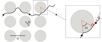
Figure 1: Schematic drawing of a sample trajectory in a pillar array with lattice constant $a$ and pillar radius $R$. The sliding and leaving angles are denoted with $\alpha$ and $\theta$, respectively.

Model.— We consider a two-dimensional medium consisting of circular pillars with radius $R$. The pillars are placed on a square lattice with lattice constant $a$. We model the motion of the self-propelled agents by a persistent random walk. The walkers move with a constant step length $l$ at each time step. We define the mean local persistence as $p\,{=}\,\langle\cos\phi\rangle$ Sadjadi and Shaebani (2021), with $\phi$ being the turning angle between the successive steps and $\langle{\cdot}{\cdot}{\cdot}\rangle$ denoting the average with respect to the turning-angle distribution $R(\phi)$. The persistence values $p=1$ and $p=0$ correspond to ballistic and purely diffusive motion, respectively. We introduce a sliding boundary condition on the pillar surfaces. After collision, the walker moves along the obstacle surface with an angle $\alpha$ and leaves the obstacle surface with angle $\theta$ from tangent of the circle; see Fig. 1. While the free parameter $\alpha$ can be pillar-size dependent in general Spagnolie et al. (2015), here we consider $\alpha$ to be independent $R$.

We perform Monte Carlo simulations of migration through the pillar park. The simulation box is $300l{\times}300l$, in which the pillars are arranged on a square lattice with lattice constant $a\,{=}\,12.5l$. A circular pillar with radius $R$ is placed on each lattice point (24 pillars in each row or column). By changing $R$, we vary the occupied fraction by pillars (characterized by the dimensionless parameter $\lambda\,{=}\,2R{/}a\,{\in}\,[0,1]$). An event-driven algorithm is applied, where every collision with an obstacle is considered as a new event. The random walker takes a step with length $l$, unless it collides with an obstacle. In case of no collision, the walker takes a new direction drawn from the turning-angle distribution $R(\phi)$, which is chosen to be a uniform function over $[\phi_{0},\phi_{1}]$. The values of the angles $\phi_{0}$ and $\phi_{1}$ can be tuned to get the desired persistence $p$. An ensemble of $10^{5}$ random walkers with random initial position and direction are considered and periodic boundary conditions are applied. To induce topotaxis, we consider a constant sliding angle $\alpha$ around each pillar but impose a gradient of $\alpha$ in the medium.

In order to understand the influence of the geometric parameters $\alpha$ and $\lambda$ on the particle migration in pillar parks, we study the behavior of the effective diffusion constant, $D$, at a given $\alpha$ and vary $\lambda$ by changing the radii of obstacles. Since the diffusion constant in free space, $D_{0}$, depends on the persistence as $D_{0}{\propto}\frac{1+p}{1-p}$ (Shaebani et al., 2014), we use the rescaled diffusion constant $\widetilde{D}{=}D{/}D_{0}$ in the following to eliminate the role of $p$. In Fig.2(a,b), $\widetilde{D}$ is plotted versus relative packing fraction $\lambda$ for different values of $\alpha$. The results are presented for diffusion ($p\,{=}\,0$) and persistent random walk with $p\,{=}\,0.5$. We observe that the diffusion constant grows with $\lambda$ and its variation is affected by the value of the sliding angle $\alpha$. Without sliding along obstacle surfaces, e.g. with reflective boundary condition on pillar surfaces, $\widetilde{D}$ decrease with pillar density, which is a known result (Dagdug et al., 2012); however, when sliding along obstacle surface is allowed, $\widetilde{D}$ interestingly increases with density. For dense packing, the displacement $R\,\!\alpha$ on the perimeter of a pillar is larger than the pillar spacing. Moreover, in denser pillar parks, where random walkers are trapped between pillars, they use the sliding on pillar surface to escape the traps and thus propagate faster between pillars. In the case of persistent random walk [Fig.2(b)], with the same $\alpha$ as for $p{=}0$, we observe a weaker increase in the relative diffusion constant. This is because active agents are less frequently trapped between pillars due to their active motion, thus, the relative impact of sliding on diffusion coefficient is less pronounced. In Fig.2(c), $\widetilde{D}$ of normal and persistent random walkers is plotted versus the sliding angle in a dense pillar park with $\lambda\,{=}\,0.96$. We observe three peaks at multiples of $\frac{\pi}{2}$. The maximum value of $\widetilde{D}$ is located either at $\alpha\,{=}\,\frac{\pi}{2}$ or $\alpha\,{=}\,\pi$, depending on the persistence of the random walker. However, this behavior disappears in smaller packing fractions, as shown for $p\,{=}\,0$ in Fig.2(d). A similar trend is observed for $p\,{>}\,0$. Thus, for sufficiently large $\lambda$, the impact of geometrical properties of the pillars (e.g. $\alpha$) on the diffusion constant are more pronounced. Based on these findings, we hypothesize that a gradient of sliding angle through the pillar park at large packing fractions can leads to topotaxis.

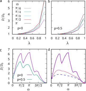
Figure 2: (a,b) Rescaled diffusion constant $D{/}D_{0}$ versus $\lambda\,{=}\,2R/a$ for a (a) normal random walk and (b) persistent walk with persistence $p\,{=}\,0.5$. Each color represents a fixed sliding angle $\alpha$ on the obstacle surface. (c) Rescaled diffusion constant as a function of sliding angle $\alpha$ for a normal and persistent random walk. (d) $D{/}D_{0}$ vs $\alpha$ for normal random walk in pillar parks with various pillar densities. The full, dotted and dashed lines represent $\lambda\,{=}\,0.96,0.8$ and $0.64$, respectively. In all cases the leaving angle $\theta$ is uniformly chosen from $[0,\frac{\pi}{4}]$.

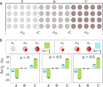
Figure 3: Inducing taxis in an obstacle park with homogeneous packing fraction by varying the sliding angle. (a) Schematic representation of an obstacle park with gradient of sliding angle $\alpha$. A different value of $\alpha$ is assigned to each zone, with zone A (C) having the smallest (largest) angle. The color intensity of pillars is proportional to $\alpha$. (b) The relative particle density in each zone (with respect to the homogeneous stationary density $\rho_{{}_{s}}$) for normal and persistent random walks for two sets of $\alpha\!_{{}_{A}},\alpha_{{}_{B}}$ and $\alpha_{{}_{C}}$ shown by green and blue colors. Here, $\lambda\,{=}\,0.96$ and $\theta$ is uniformly chosen from $[0,\frac{\pi}{4}]$.

In order to induce topotaxis in a homogeneous medium with uniform packing fraction, we consider a mono-disperse pillar park and assume that the sliding angle of particles along pillars is an angle which can be tuned by adapting the surface properties, e.g. by means of different coatings. We divide the pillar park into parallel sections and assign a constant sliding angle to each section. Here, we present the results for choosing three zones $A$, $B$, and $C$ with $\alpha\!_{{}_{A}}\,{<}\,\alpha_{{}_{B}}\,{<}\,\alpha_{{}_{C}}$, as depicted in Fig.3(a). Note that due to periodic boundary condition, sections A and C are also neighbors. We define particle density $\rho$ as the number of random walkers per unit of available area (i.e. pillar area excluded). We let the random walkers migrate in the pillar park, starting from random positions and orientations. In a homogeneous pillar park, one expects to have $\rho\!_{{}_{A}}\,{=}\,\rho_{{}_{B}}\,{=}\,\rho_{{}_{C}}\,{\equiv}\,\rho_{{}_{s}}$, with $\rho_{{}_{s}}{=}\,\frac{1}{3}$ being the particle density in the steady state of a homogeneous pillar park. Here, we observe $\rho\!_{{}_{A}}\,{<}\,\rho_{{}_{B}}\,{<}\,\rho_{{}_{C}}$, which means that the random walkers preferentially reside in the zones with larger sliding angles. Interestingly, this tendency mainly depends on the values of sliding angles (in a given $\lambda$) rather than the persistence of the random walker. A larger difference $\Delta\alpha$ between the sliding angles in adjacent zones results in a larger difference in the steady particle densities $\rho\!_{{}_{A}}$, $\rho_{{}_{B}}$, and $\rho_{{}_{C}}$. In Fig.3(b), exemplary variations of the relative density $\Delta\rho\,{=}\,\rho-\rho_{{}_{s}}$ are shown in different zones in the steady state. The results are presented for $p\,{=}\,0$, $0.2$ and $0.5$ and two sliding angles $\alpha\!_{{}_{A}}$, $\alpha_{{}_{B}}$ and $\alpha_{{}_{C}}$ as depicted by red color in the figure. For simplicity, we assume that the differences between sliding angles in the two neighboring zones are the same, i.e. $\Delta\alpha\,{=}\,|\alpha\!_{{}_{A}}{-}\,\alpha_{{}_{B}}|\,{=}\,|\alpha_{{}_{B}}{-}\,\alpha_{{}_{C}}|\,{=}\,\frac{1}{2}|\alpha\!_{{}_{A}}{-}\,\alpha_{{}_{C}}|$. In examples shown in Fig.3(b) with green ad blue colors, $\Delta\alpha$ equals $\frac{\pi}{2}$ and $\frac{\pi}{4}$, respectively. For all choices of persistence $p$, a positive (negative) $\Delta\rho$ in section $C$ ($A$) in the steady state shows that more (less) particles are found there. Moreover, a larger $\Delta\alpha$ (green) results in a significantly larger $|\Delta\rho/\rho_{{}_{s}}|$, compared to the one with a smaller $\Delta\alpha$ (blue). This result indicates a taxis from smaller to larger $\alpha$ with a strength which depends on $\Delta\alpha$. We checked that other (inhomogeneous) initial conditions lead to similar conclusions. The result illustrated by Fig.3(b) is somewhat counter-intuitive, since sliding with larger angles is reminiscent of active particles attaining higher activity or self-propulsion— which leads in active Brownian particle systems to a depletion of particles Wysocki et al. (2022), contrary to what happens here— and we will clarify the reason below.

To better understand how the topotaxis strength depends on $\Delta\alpha$ as well as the pillar packing fraction $\lambda$, we quantify the strength of taxis $\Gamma$ by the maximum difference between the steady densities, i.e. $\Gamma\,{=}\,\rho_{{}_{C}}\,{-}\,\rho\!_{{}_{A}}$. In Fig.4(a), $\Gamma$ is plotted versus $\Delta\alpha$ for different values of $\lambda$ for a given $p$. We set $\alpha_{{}_{C}}{=}\,\pi$ and vary $\Delta\alpha$ (i.e. choose $\alpha\!_{{}_{A}}\,{=}\,\pi\,{-}\,2\Delta\alpha$ and $\alpha\!_{{}_{B}}\,{=}\,\pi\,{-}\,\Delta\alpha$). $\Gamma$ shows a nearly linear dependence on $\Delta\alpha$ which is stronger for larger $\lambda$. Even for middle values of $\lambda$, a significant topotaxis can be achieved by choosing proper parameters. Figure 4(b)

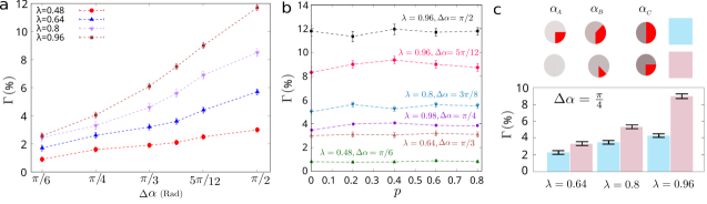
Figure 4: (a) Topotaxis strength $\Gamma$ versus $\Delta\alpha$ for $p\,{=}\,0.6$ and different values of $\lambda$. (b) $\Gamma$ vs persistence $p$ of random walker for various choices of $\lambda$ and $\Delta\alpha$. (c) Topotaxis strength for $\Delta\alpha\,{=}\,\frac{\pi}{4}$ and two different choices of sliding angles. Here, $p\,{=}\,0.6$ and the results are shown for three values of $\lambda$.

shows $\Gamma$ versus $p$ for various choices of $\lambda$ and $\Delta\alpha$. It can be clearly seen that $\Gamma$ is independent of persistence, while it strongly depends on the choice of the geometrical parameters $\lambda$ and $\Delta\alpha$. We note that for a given choice of $\Delta\alpha$, there is a degree of freedom to choose the set of the sliding angles of the zones. An example for $\Delta\alpha\,{=}\,\frac{\pi}{4}$ and two choices of sliding angles is shown In Fig.4(c). Interestingly, $\Gamma$ depends not only on $\Delta\alpha$ but also on the chosen range of the sliding angles. Denoting the minimum sliding angle by $\alpha_{\text{min}}\,{\equiv}\,\alpha\!_{{}_{A}}$, we observe that choosing a smaller $\alpha_{\text{min}}$ leads to a larger $\Gamma$. Thus, for given values of $\Delta\alpha$ and $\lambda$, the maximum topotaxis strength is achieved for $\alpha_{\text{min}}\,{=}\,0$, i.e. no sliding on the pillars.

In an inhomogeneous environment, random walkers tend to gather in regions where they have a lower mobility, i.e. smaller diffusion constant Schnitzer (1993). Therefore, the trivial way to induce topotaxis is to apply a gradient of packing fraction of obstacles, which changes the local available space for migration. This way, the density of particles will be higher in regions with larger obstacle packing fraction, where particles have smaller $D$ due to frequent reflections. However, our findings demonstrate a counterintuitive possibility. We induce accumulation in zones with larger sliding angles, which have a larger diffusion constant [see Fig.2(c)]. To provide a qualitative understanding of the underlying mechanism, we focus on the interface between two zones with different sliding angles $\alpha_{1}\,{<}\,\alpha_{2}$. In Fig.5(a), a sample trajectory in the extreme case of $\alpha_{1}\,{=}\,0$ and $\alpha_{2}\,{=}\,\pi$ is depicted. Starting in region $1$ (i.e. left), the particle is often trapped between the obstacles due to frequent reflections from them. However, when it enters region 2 with the possibility of sliding on pillars, it can be effectively pulled into the medium by sliding around many pillar surfaces without being locally trapped. If one waits enough, the particle returns to the interface again, as shown in Fig.5(b) for different choices of $p$, $\alpha_{1}$, and $\alpha_{2}$. While these sample random walkers have the chance to reenter region 1, the interface acts as a pseudo-reflective wall and effectively guides the walkers back to region 2.

Towards practical applications, such as guiding biological agents inside channels, particles should be guided in a specified direction over long distances. To this aim, one could partition the system into many blocks with successively increasing $\alpha$. However, this corresponds to small $\Delta\alpha$ between neighboring blocks, thus, a weak effective topotaxis strength $\Gamma$ [see Fig.4(a)]; indeed, $\Gamma{\rightarrow}0$ for $\Delta\alpha{\rightarrow}0$. We exploit this feature by linearly decreasing $\alpha$ from $\pi$ to $0$ in each block as shown in Fig.5(c). As a result, while the particles experience no significant topotaxis within each block, they are pulled into the neighboring block at the interface with $\Delta\,\alpha\,\,{=}\,\pi$. When

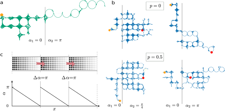
Figure 5: (a) An exemplary trajectory at the interface of two zones with different $\alpha$. The starting point is depicted by the orange circle. (b) Examples of longer trajectories where the random walker has enough time for several returns to the interface. Different panels represent either normal or persistent random walks for two choices of sliding angles $\alpha_{1}$ and $\alpha_{2}$. The orange and red circles represent the starting and final position of the random walker, respectively. (c) Schematic design for guiding particles through blocks of pillars with a linear decrease of $\alpha$ in each block, represented with decreasing color intensity. Red arrows show the direction of the net flux.

measures the net flux (by counting the number of particles crossing the interfaces between blocks in both directions) in the simulation box, one obtains a significant flux of particles in the steady state, from left to right.

We note that the values of $\alpha_{1}$ and $\alpha_{2}$ and the trajectories in Fig.5 have been selected to highlight the effective reflection at the interface. Nevertheless, transport occurs in both directions in general, though with asymmetric probabilities $f\!_{{}_{1{\rightarrow}2}}$ and $f\!_{{}_{2{\rightarrow}1}}$ which depend on the geometrical parameters $\Delta\alpha$, $\alpha_{\text{min}}$, and $\lambda$ but are independent of $p$. The Markov process of transport between these two zones eventually leads to steady state probabilities $\rho_{{}_{1}}{=}f\!_{{}_{2{\rightarrow}1}}/(f\!_{{}_{1{\rightarrow}2}}+f\!_{{}_{2{\rightarrow}1}})$ and $\rho_{{}_{2}}{=}f\!_{{}_{1{\rightarrow}2}}/(f\!_{{}_{1{\rightarrow}2}}+f\!_{{}_{2{\rightarrow}1}})$ for residence in each zone. Although the explicit dependence of transition probabilities on topological properties of the medium is not known, their asymmetry is reflected in their ratio in the steady state, which is given as $\frac{f\!_{{}_{1{\rightarrow}2}}}{f\!_{{}_{2{\rightarrow}1}}}{=}\frac{\rho_{2}}{\rho_{1}}$. An strong topotaxis is gained for the set of conditions $\{\lambda{\rightarrow}1$, $\Delta\alpha{\gg}0$, and $\alpha_{\text{min}}{\rightarrow}0\}$. On the other hand, in sparse pillar parks (i.e. $\lambda{\ll}1$) or in the limit of $\Delta\alpha{\rightarrow}0$, we obtain $\rho_{{}_{1}}{\approx}\rho_{{}_{2}}{\approx}\rho_{{}_{s}}$ corresponding to a very weak topotaxis. As a final note, while the persistence affects neither the transition probabilities nor the steady densities, it determines the time scale to reach the steady state; a particle with a larger $p$ visits the interface more frequently as it has a larger diffusion coefficient.

In summary, we have proposed a novel method to induce topotaxis in obstacle parks with a uniform packing fraction, by applying a gradient in the angle of sliding around pillars. We verified that the method is capable of guiding agents over long distances. The concept can be generalized to other characteristics of agent-obstacle interactions or other geometrical properties of the environment. For example, we have preliminary results showing that topotaxis can be also achieved in the absence of sliding by imposing a gradient of a degree of pillar-size polydispersity in the environment. The persistence dependence of the relaxation time to the steady state can be exploited to separate a mixture of microorganisms with different persistence. Our results are of technological importance as a non-invasive method (e.g. by imposing different pillar-surface coatings) to design taxis devices for guiding biological agents.

This work was performed within and financially supported by the Collaborative Research Center SFB 1027 funded by the German Research Foundation (DFG).

References

- Park et al. (2018) J. Park, D.-H. Kim, and A. Levchenko, Biophys. J. 114, 1257 (2018).
- Wondergem et al. (2021) J. A. J. Wondergem, M. Mytiliniou, F. C. H. de Wit, T. G. A. Reuvers, D. Holcman, and D. Heinrich, bioRxiv p. doi:10.1101/735779 (2021).
- Reversat et al. (2020) A. Reversat et al., Nature 582, 582 (2020).
- Gorelashvili et al. (2014) M. Gorelashvili, M. Emmert, K. F. Hodeck, and D. Heinrich, New J. Phys. 16, 075012 (2014).
- Schakenraad et al. (2020) K. Schakenraad, L. Ravazzano, N. Sarkar, J. A. J. Wondergem, R. M. H. Merks, and L. Giomi, Phys. Rev. E 101, 032602 (2020).
- Frey et al. (2006) M. T. Frey, I. Y. Tsai, T. P. Russell, S. K. Hanks, and Y. li Wang, Biophys. J. 90, 3774 (2006).
- Kaiser et al. (2006) J.-P. Kaiser, A. Reinmann, and A. Bruinink, Biomaterials 27, 5230 (2006).
- (8) M. J. Muthinja et al. (????).
- Chabaud et al. (2015) M. Chabaud et al., Nat. Commun. 6, 7526 (2015).
- Shaebani et al. (2020) M. R. Shaebani, R. Jose, L. Santen, L. Stankevicins, and F. Lautenschläger, Phys. Rev. Lett. 125, 268102 (2020).
- Maiuri et al. (2015) P. Maiuri et al., Cell 161, 374 (2015).
- Shaebani et al. (2022) M. R. Shaebani et al., Biophy. J. 121, 3950 (2022).
- Stankevicins et al. (2020) L. Stankevicins et al., Proc. Natl. Acad. Sci. USA 117, 826 (2020).
- Shaebani et al. (2022a) M. R. Shaebani, M. Piel, and F. Lautenschläger, Biophys. J. 121, 4099 (2022a).
- Spagnolie et al. (2015) S. E. Spagnolie, G. R. Moreno-Flores, D. Bartolo, and E. Lauga, Soft Matter 11, 3396 (2015).
- Jakuszeit et al. (2019) T. Jakuszeit, O. A. Croze, and S. Bell, Phys. Rev. E 99, 012610 (2019).
- Sipos et al. (2015) O. Sipos, K. Nagy, R. Di Leonardo, and P. Galajda, Phys. Rev. Lett. 114, 258104 (2015).
- Sadjadi et al. (2022) Z. Sadjadi, D. Vesperini, A. M. Laurent, L. Barnefske, E. Terriac, F. Lautenschläger, and H. Rieger, Biophys. J. 121, doi:10.1016/j.bpj.2022.10.030 (2022).
- Arcizet et al. (2012) D. Arcizet, S. Capito, M. Gorelashvili, C. Leonhardt, M. Vollmer, S. Youssef, S. Rappl, and D. Heinrich, Soft Matter 8, 1473 (2012).
- Zhou et al. (2017) X. Zhou, R. Zhao, K. Schwarz, M. Mangeat, E. C. Schwarz, M. Hamed, I. Bogeski, V. Helms, H. Rieger, and B. Qu, Sci. Rep. 7, 44357 (2017).
- Kantsler et al. (2013) V. Kantsler, J. Dunkel, M. Polin, and R. E. Goldstein, Proc. Natl. Acad. Sci. USA 110, 1187 (2013).
- Lushi et al. (2017) E. Lushi, V. Kantsler, and R. E. Goldstein, Phys. Rev. E 96, 023102 (2017).
- Contino et al. (2015) M. Contino, E. Lushi, I. Tuval, V. Kantsler, and M. Polin, Phys. Rev. Lett. 115, 258102 (2015).
- Saxton (1987) M. J. Saxton, Biophys. J. 52, 989 (1987).
- Saxton (1994) M. J. Saxton, Biophys. J. 66, 394 (1994).
- Machta and Zwanzig (1983) J. Machta and R. Zwanzig, Phys. Rev. Lett. 50, 1959 (1983).
- Sadjadi et al. (2008) Z. Sadjadi et al., Phys. Rev. E 78, 031121 (2008).
- Tierno et al. (2016) P. Tierno et al., Soft Matter 12, 3398 (2016).
- Dagdug et al. (2012) L. Dagdug, M.-V. Vazquez, A. M. Berezhkovskii, V. Y. Zitserman, and S. M. Bezrukov, J. Chem. Phys. 136, 204106 (2012).
- Shaebani et al. (2022b) M. R. Shaebani, H. Rieger, and Z. Sadjadi, Phys. Rev. E 106, 034105 (2022b).
- Hafner et al. (2016) A. Hafner et al., Sci. Rep. 6, 37162 (2016).
- Shaebani and Rieger (2019) M. R. Shaebani and H. Rieger, Front. Phys. 7, 120 (2019).
- Sadjadi and Shaebani (2021) Z. Sadjadi and M. R. Shaebani, Phys. Rev. E 104, 054613 (2021).
- Shaebani et al. (2014) M. R. Shaebani, Z. Sadjadi, I. M. Sokolov, H. Rieger, and L. Santen, Phys. Rev. E 90, 030701 (2014).
- Wysocki et al. (2022) A. Wysocki, A. K. Dasanna, and H. Rieger, N. J. Phys. 24, 093013 (2022).
- Schnitzer (1993) M. J. Schnitzer, Phys. Rev. E 48, 2553 (1993).