Scalable noisy quantum circuits for biased-noise qubits

Abstract

In this work, we consider biased-noise qubits affected only by bit-flip errors, which is motivated by existing systems of stabilized cat qubits. This property allows us to design a class of noisy Hadamard-tests involving entangling and certain non-Clifford gates, which can be conducted reliably with only a polynomial overhead in algorithm repetitions. On the flip side we also found classical algorithms able to efficiently simulate both the noisy and noiseless versions of our specific variants of Hadamard test. We propose to use these algorithms as a simple benchmark of the biasness of the noise at the scale of large circuits. The bias being checked on a full computational task, it makes our benchmark sensitive to crosstalk or time-correlated errors, which are usually invisible from individual gate tomography. For realistic noise models, phase-flip will not be negligible, but in the Pauli-Twirling approximation, we show that our benchmark could check the correctness of circuits containing up to $10^{6}$ gates, several orders of magnitudes larger than circuits not exploiting a noise-bias. Our benchmark is applicable for an arbitrary noise-bias, beyond Pauli models.

Quantum computers bring the hope of solving useful problems for society that would be out of reach from classical supercomputers. One can think of problems in optimisation [1, 2], cryptography [3, 4], finance [5, 6], quantum chemistry or material science [7, 8, 9, 10, 11]. The main threats toward the realization of useful quantum computers are noise and decoherence [12] which cause errors and degrade the quality of the computation. In the long term this problem will likely be addressed by quantum error correction and fault-tolerant quantum computing [13, 14, 15, 16, 17, 13, 18]. Yet, the very high fidelity and considerable overhead this approach requires makes it very challenging to implement.

In this context, the existence of quantum algorithms able to scale up to large size, with a hardware of low fidelity would be highly desirable. Unfortunately, various studies showed that polynomial-time classical algorithms can efficiently simulate the algorithm outputs of specific circuits in the noisy case, such as random circuits [19, 20] or general algorithms under some assumptions on the noise structure [21, 22, 23] (see also [24] and [25, 26] for analogous results in the optical setting). All these studies indicate that without doing error-correction, for realistic noise models, it is not possible to preserve reliable algorithm outputs in a classically intractable regime (see however recent work [27], which showed that in certain oracular scenarios noisy quantum computers can offer an advantage over classical computers). One major difficulty to face is that, for most noise models, the fidelity of the output state drops exponentially with the number of gates involved in the computer [28] suggesting that a reliable estimation of any expectation value would require to run exponentially many times the algorithm, ruining any hope for an exponential speedup. Error mitigation techniques [29, 30, 31, 32, 33, 34, 35, 36] have been proposed, with the hope to solve this issue. However various no-go results show that, for several noise models, error mitigation techniques are not scalable [33, 37]: the number of samples they require can grow exponentially with the algorithm’s depth or the number of qubits in the algorithm [38, 34, 39]. Other approaches can be potentially more scalable, but they assume specific noise models [40], require knowledge of entanglement spectrum of quantum states [41] or have potentially high algorithmic complexity [42].

In our work, motivated by the limitations of error-correction and error mitigation, we propose instances of the Hadamard test [43, 44] that can be robustly implemented in systems of so-called biased-noise qubits [45, 46, 47], affected only by local stochastic bit flip (or phase-flip) errors. In technical terms, we show that, for suitably designed circuits tailored to a Pauli biased noise the outcome of the ideal version of the Hadamard test can be estimated reliably by execution of its noisy versions with only a polynomial overhead in the number of repetitions of the algorithm. The model of biased-noise qubits is motivated by existing hardware realising stabilized cat qubits [46, 48, 47]. The key ingredient of our approach is that only specific gates are allowed, in order to preserve the noise bias along the computation [45, 49]. This allows us to design circuits in which the measurement will be isolated from most of the errors occurring (see Fig. 1). Importantly, the circuits themselves can be quite complicated, generate large amounts of entanglement and contain certain non-Clifford gates, thus avoiding natural classical simulation techniques [50, 51, 52]. Nonetheless, the restricted nature of these circuits allowed us to find an efficient classical algorithm that simulates (noiseless) realisations of our family of Hadamard tests. We propose to use this algorithm as a simple benchmark of the biasness of the noise at the scale of large and complicated quantum circuits, allowing to check the hardware reliability in presence of correlated noise, which would be invisible from individual gate tomography. For simplicity, in the main text, we focus on the case of Pauli noise, but our benchmark is extended in supplemental D.4 for the most general model of local biased noise.

Notation. Let $(\sigma_{0},\sigma_{1},\sigma_{2},\sigma_{3})\equiv(I,X,Y,Z)$ denote single qubit Pauli matrices. Let $H$ denote the Hadamard gate. We call $\mathbb{P}_{n}^{X}$ the set of $X$-Pauli operators acting on $n$-qubits, $\mathbb{P}_{n}^{X}\equiv\{\bigotimes_{k=1}^{n}\sigma_{i_{k}},\leavevmode\nobreak\ |\forall k,i_{k}\in\{0,1\}\}$. We say that $f_{n}\in\text{poly}(n)$ if there exists two reals $C,a>0$ such that $\lim_{n\to\infty}f_{n}/(Cn^{a})=1$. Moreover, when $\text{poly}(n)$ appears in an equation, it means that the equation remains true by replacing $\text{poly}(n)$ by any function $f_{n}\in\text{poly}(n)$. Lastly, we say that $f_{n}=O(g_{n})$ if there exists $C>0$ such that $\lim_{n\to\infty}|f_{n}/g_{n}|\leq C$. For any unitary $U$, we define its coherently controlled operation in the $X$-basis as $c_{X}U\equiv{|+\rangle\langle+|}\otimes I+{|-\rangle\langle-|}\otimes U$. Let $G$ be a single-qubit unitary. $G_{i}$ indicates that $G$ is applied on the $i$’th qubit in the tensor product (and $I$ is applied elsewhere).

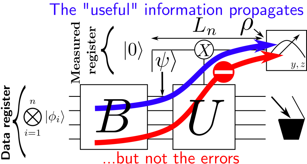
Figure 1: The Hadamard test represented on this figure allows to estimate $\bra{\psi}U\ket{\psi}$ where $\ket{\psi}\equiv B\bigotimes_{i=1}^{n}\ket{\phi_{i}}$, ($\ket{\phi_{i}}$ being a single-qubit state, $B$ a unitary). This estimation is being done by initializing a measured register in $\ket{0}$, and by implementing the unitary $c_{X}U$. Finally, measuring the measured register in Pauli $Y$ and $Z$ bases gives access to the imaginary and real part of $\bra{\psi}U\ket{\psi}$. We call $L_{n}$ the number of gates applied on the measured register (including potential noisy identity gates), once $c_{X}U$ has been decomposed on an experimentally feasible gateset. In this paper, we show that for a noise model only composed of bit-flips, and under some restrictions on the $n$-qubit unitaries $U$ and $B$, the measurement will only be sensitive to bit-flips produced on the measured register, and entirely insensitive to the ones produced on the data register. Nonetheless, some ”useful information” contained in the entangled state $\ket{\psi}$ will propagate toward the measurement. The intuitive principle we use is to encode the ”useful” information in a ”Pauli $Z$ (or $Y$) channel” while making sure that any error is inside a ”Pauli $X$ channel”. If any Pauli $X$ error (i.e. bit-flip) from the data register cannot propagate toward the measurement while the Pauli $Z$ can, the information will reach the measurements but not the errors. Overall, if $L_{n}=O(\log(n))$, the noise will only introduce a polynomial overhead in the number of algorithm repetitions to guarantee a reliable outcome: the algorithm will be scalable despite the noise. Note that while $L_{n}=O(\log(n))$, the algorithm can nonetheless have a polynomial depth.

The Hadamard test. The Hadamard test is the task over which all our examples are built. It allows to estimate the expectation value $\bra{\psi}U\ket{\psi}$ of a unitary $U$ on some prepared $n$-qubit state $\ket{\psi}=B\bigotimes_{i=1}^{n}\ket{\phi_{i}}$ ($\ket{\phi_{i}}$ being a single-qubit state, $B$ a unitary operation), leading to several applications [53, 54, 44]. A way to implement it is represented in Fig. 1. It consists of a ”measured” register initialized in $\ket{0}$ combined with a ”data” register, where the state $\ket{\psi}$ has been prepared. The reduced state of the measured register right before measurement takes the following form

$$\rho=\frac{1}{2}\left(I+\alpha_{n}\left(yY+zZ\right)\right)\,$$ (1)

where $y=-\imaginary(\bra{\psi}U\ket{\psi}),z=\real(\bra{\psi}U\ket{\psi})$ and $\alpha_{n}=1$ for now on. Hence, measuring the first register in the $Y$ (resp $Z$) basis allows to estimate the imaginary (resp real) part of $\bra{\psi}U\ket{\psi}$. Using Hoeffding’s inequality [33] we get that $N=2\log(2/\delta)/\epsilon^{2}$ experimental repetitions are sufficient to estimate $y$ or $z$ up to $\epsilon$-precision with a probability $1-\delta$. It is well-known that estimating $\bra{\psi}U\ket{\psi}$, for a general polynomial circuit $U$, to additive precision is a BQP complete problem [53] and therefore in general we do not expect an efficient classical algorithm that would be realising this task.

So far, we discussed what happens when the measured qubit is noiseless. Let us now assume that a bit-flip channel right before the measurement occurs in such a way that $0<\alpha_{n}<1$ in Eq. (1). Then, repeating the algorithm $N_{n}=2\log(2/\delta)/(\alpha_{n}\epsilon)^{2}$ times would be sufficient to estimate $y$ and $z$ to $\epsilon$ precision with high probability (the scaling in $1/(\alpha_{n}\epsilon)^{2}$ is also optimal). If $\alpha_{n}$ decreases exponentially with $n$, the total number of algorithm calls will necessarily grow exponentially with $n$ and the algorithm wouldn’t be scalable. However, for $\alpha_{n}=1/\text{poly}(n)$, only $\text{poly}(n)$ overhead in experiment repetitions would be sufficient to reliably estimate $\bra{\psi}U\ket{\psi}$. In this work, we will show that for biased-noise qubits it is possible to design a class of non-trivial Hadamard tests for which $\alpha_{n}=1/\text{poly}(n)$ in the presence of non-vanishing local biased noise.

Noise model. In general, both $B$, and $c_{X}U$ have to be decomposed on a gateset implementable at the experimental level. Let $\mathcal{G}$ be a unitary channel describing a gate belonging to the accessible gateset, and $\mathcal{E}_{\mathcal{G}}$ be its noisy implementation in the laboratory. We will assume a local biased noise model: $\mathcal{E}_{\mathcal{G}}=\mathcal{N}_{\mathcal{G}}\circ\mathcal{G}$, where the ”noise map” $\mathcal{N}_{\mathcal{G}}$ will only introduce (possibly correlated) bit-flip errors on the qubits on which $\mathcal{G}$ acts non-trivially (i.e. $\mathrm{supp}(\mathcal{G})$),

$$\mathcal{N}_{\mathcal{G}}(\rho)=\sum_{\alpha\subset\mathrm{supp}(\mathcal{G})}p^{\mathcal{G}}_{\alpha}X_{\alpha}\rho X_{\alpha}\ ,$$ (2)

where $X_{\alpha}=\prod_{i\in\alpha}X_{i}$ and $\{p^{\mathcal{G}}_{\alpha}\}$ is a probability distribution supported on subsets of $\mathrm{supp}(\mathcal{G})$. For instance, the noise model of a two-qubit gate will have Kraus operators proportional to $\sigma\otimes\sigma^{\prime}$ with $(\sigma,\sigma^{\prime})\in\{I,X\}$. Furthermore, a noisy measurement is modelled by a perfect measurement followed by a probability $p_{\text{meas}}$ to flip the outcome. Lastly, we assume that single-qubit noisy state preparation consists of a perfect state preparation followed by the application of a Pauli $X$-error with probability $p_{\text{prep}}$. Our noise model is based on an idealization of cat qubits that are able to exponentially suppress other noise channels than bit-flip, at the cost of a linear increase in bit-flip rate [46, 48, 47] (or the other way around). It is an idealization as (i) our Kraus operators can be decomposed with $X$ and $I$ operators only: this is what we call a perfect bias, (ii) we also neglect coherent errors. In supplemental D.4, we show that our main result (the benchmarking protocol) can be extended to work with an arbitrary local biased noise model (i.e. the noise is not necessarily Pauli). We now provide the definition of ”an error”.

Definition 1 (Error).

Let $\ket{\Psi}$ be the state the qubits should be in at some timestep of the algorithm if all the gates were perfect. Because we consider a probabilistic noise model, the actual $n$-qubit quantum state will take the form $\rho=\sum_{i}p_{i}E_{i}\ket{\Psi}\bra{\Psi}E_{i}^{\dagger}$, where $E_{i}$ is a unitary operator and $p_{i}$ some probability ($p_{i}\geq 0$, $\sum_{i}p_{i}=1$). The operator $E_{i}$ is what we call the error that affected $\ket{\Psi}$.

Noise-resilient Hadamard test. The core idea behind our work is to exploit the fact that only bit-flips are produced, in order to design circuits guaranteeing that most of these errors will never reach the measurement in the Hadamard test. In order to explain our results we need to introduce first a number of auxiliary technical definitions.

Definition 2 ($X$-type unitary operators and errors).

We call $X$-type unitary operators the set of unitaries that can be written as a linear combination of Pauli $X$ matrices. For $n$-qubits, we formally define it as:

$$\mathbb{U}_{n}^{X}\equiv\{U=\sum_{i}c_{i}P_{i},\leavevmode\nobreak\ |P_{i}\in\mathbb{P}_{n}^{X},c_{i}\in\mathbb{C},U^{\dagger}=U^{-1}\},$$ (3)

Alternatively, $\mathbb{U}_{n}^{X}$ can be understood in terms of unitaries that are diagonal in the product basis $\ket{\mathbf{s}}=\ket{s_{1}}\ket{s_{2}}\ldots\ket{s_{n}}$, where $s_{i}=\pm$ and $\ket{\pm}$ are eigenstates of Pauli $X$ matrix. We will call ”$X$-error”, an error belonging to $\mathbb{U}_{n}^{X}$ (if the error is additionally Pauli, we will call it ”Pauli $X$ error”, or simply ”bit-flip”).

What we need to do is to guarantee that any error occurring at any step of the computation is an $X$-error. It is possible with the use of ”bias-preserving” gates: such gates map any initial $X$-error to another $X$-error. It motivates the following definition and property (all our results are derived in the Supplemental material).

Definition 3 (Bias-preserving gates).

Let $G$ be an $n$-qubit unitary operator. We say that $G$ preserves the $X$-errors (or $X$-bias), if it satisfies the following property

$$\forall P\in\mathbb{P}_{n}^{X},\exists A\in\mathbb{U}_{n}^{X}\text{ such that }GP=AG$$ (4)

We denote $\mathbb{B}_{n}$ the set of such gates.

Property 1 (Preservation of the bias).

If a quantum circuit is only composed of gates in $\mathbb{B}_{n}$, each subject to local biased noise model from Eq. (2) (and the paragraph that follows for measurement and preparation), then any error affecting the state of the computation is an $X$-error.

As examples of bias-preserving gates, there are all the unitaries in $\mathbb{U}_{n}^{X}$, the cNOT, and what we call $\text{Toffoli'}\equiv H_{1}H_{2}H_{3}\times\text{Toffoli}\times(H_{1}H_{2}H_{3})^{\dagger}$. An example of a gate that does not preserve the bias is the Hadamard gate. The existence of gate preserving the bias also during the gate implementation is not straightforward, but cat-qubits are able to overcome this complication, at least for cNOT, Toffoli’ and gates in $\mathbb{U}_{n}^{X}$: see the section A.3 in the Supplemental Material. Finally, bias preserving gates have a nice interpretation: they correspond to permutations (up to a phase) in the Pauli $X$-eigenstates basis.

Property 2 (Characterization of bias-preserving gates).

$V\in\mathbb{B}_{n}$ if and only if for any $\mathbf{s}\in\{{+,-\}}^{n}$, there exists a real phase $\varphi_{\mathbf{s},V}$ such that: $V\ket{\mathbf{s}}=e^{i\varphi_{\mathbf{s},V}}\ket{\sigma_{V}(\mathbf{s})}$ where $\sigma_{V}$ is some permutation acting on $\{{+,-\}}^{n}$.

We now sketch the sufficient ingredients guaranteeing the existence of noise-resilient Hadamard tests. First, (i) assume that individual gate errors, as well as individual measurement and state-preparation errors, occur with a probability smaller than $p<1/2$. Furthermore, assume (ii) that only $X$-errors occur in the algorithm (it can be satisfied with the assumptions of Property 1), (iii) these errors cannot propagate from the data to the measured register, (iv) the number of interactions of the measured register with the data register satisfies $L_{n}=O(\log(n))$ (which implies the measured register will only be impacted by $X$-errors introduced at $O(\log(n))$ locations). Subject to conditions (i-iv) the reduced state $\rho$ will satisfy Eq. (1) with $\alpha_{n}$ efficiently computable classically, and satisfying $\alpha_{n}\geq 1/\text{poly}(n)$. As explained earlier, this would guarantee a scalable algorithm to estimate $\bra{\psi}U\ket{\psi}$. More formally, the following Theorem holds.

Theorem 1 (Hadamard test resilient to biased noise).

Let:

$$\ket{\psi}=B\bigotimes_{i=1}^{N_{B}}\ket{\phi_{i}},\ U=W\cdot V\ ,$$

$$\ W\equiv\prod_{i=1}^{N_{W}}W_{i},\ V\equiv\prod_{i=1}^{N_{V}}V_{i}\ ,$$ (5)

where $B$ is a product of local bias preserving gates, gates $V_{i}$ and $W_{i}$ are local gates and belong to $\mathbb{U}_{n}^{X}$. Additionally, the gates $W_{i}$ are assumed to be Hermitian.

Furthermore, we assume the local bias noise model introduced in Eq. (2), and that state preparation, measurements, and each non-trivial gate applied on the measurement register have a probability at most $p<1/2$ to introduce a bit-flip on the measured register.

Under these conditions, there exists a quantum circuit realising a Hadamard test such that, in the presence of noise, the reduced state $\rho$ satisfies Eq. (1) with $\alpha_{n}\geq(1-2p)^{O(N_{V})}$.

Additionally, $\alpha_{n}$ is efficiently computable classically. Hence, if $N_{V}=O(\log(n))$, it is possible to implement the Hadamard test in such a way that running the algorithm $\text{poly}(n)$ times is sufficient to estimate the real and imaginary parts of $\bra{\psi}U\ket{\psi}$ to $\epsilon$ precision with high probability.

To get intuition on how the allowed circuits are built, the reader can look at Figure 4 in the Supplemental Material. We should emphasize that Theorem 1 allows us to implement noise resilient Hadamard tests with $U$ acting non-trivially on all the qubits in the data register. While Theorem 1 assumes the trivial identity gate to be noiseless, the results can be extended if they are noisy (in this case, $W$ should have a depth in $O(\log(n))$, as discussed in the section C.3 of the Supplemental Material). Our approach is also scalable in the presence of noisy measurements (measuring the data register in the $X$ basis to infer $\bra{\psi}U\ket{\psi}$ would not be scalable in general in this case: see [56] and the section D.2 of the Supplemental Material).

Efficient simulation of noise-resilient Hadamard test and benchmarking protocol. We just saw that restricted forms of Hadamard tests are resilient to bit-flip errors occurring throughout the circuit. The following result proves that the task realised by such a restricted Hadamard test can be efficiently simulated on a classical computer with polynomial effort.

Theorem 2 (Efficient classical simulation of restricted Hadamard test).

Let $B\in\mathbb{B}_{n},U\in\mathbb{U}^{X}_{n}$ be n qubit unitaries specified by $R_{B}$ and $R_{U}$ local qubit gates (belonging to respective classes $\mathbb{B}_{n}$ and $\mathbb{U}^{X}_{n}$). Let $\ket{\psi_{0}}=\ket{\phi_{1}}\ket{\phi_{2}}\cdots\ket{\phi_{n}}$ be an initial product state. Then, there exists a randomized classical algorithm $\mathcal{C}$, taking as input classical specifications of circuits defining $B$, $U$, and the initial state $\ket{\psi_{0}}$, that efficiently and with a high probability computes an additive approximation to $\bra{\psi_{0}}B^{\dagger}UB\ket{\psi_{0}}$. Specifically, we have

$$\Pr\left(|\bra{\psi_{0}}B^{\dagger}UB\ket{\psi_{0}}-\mathcal{C}|\leq\epsilon\right)\geq 1-\delta\ ,$$ (6)

while the running time is $T=O\left(\frac{R_{B}+R_{U}+n}{\epsilon^{2}}\log(1/\delta)\right)$.

The classical simulability of the restricted Hadamard test can be regarded as the limitation of our approach to construct quantum circuits that are robust to biased noise. At the same time, it allows us to introduce an efficient and scalable benchmarking protocol that is tailored at validating the assumption of bias noise on the lever of the whole (possibly complicated) circuit.

Let us sketch the certification protocol suggested by the above classical simulation algorithm (for simplicity of the presentation we avoid detailed analysis of its sampling complexity). At the begining we need to perform tomography on the gates that need to be applied on the measured register, in order to find the probability that each such gate introduces a bit-flip on the measured register. Other noise parameters $p_{\text{meas}}$ and $p_{\text{prep}}$ would also need to be estimated. Then, a Hadamard test satisfying the constraints of Theorem 1 is chosen. Subsequently, one needs to classically compute $\alpha_{n}$, and estimate $y,z$ up to $\epsilon$-precision, with high probability (using Theorem 2). The estimates of the noiseless $y,z$ are compared to values of $Tr(\rho Y)/\alpha_{n}$, $Tr(\rho Z)/\alpha_{n}$ estimated experimentally by running the quantum circuit polynomially many times. The experimental and theoretical predictions are then compared. If they don’t match (up to error resulting from a finite number of experiments), it would necessarily indicate a violation of the assumptions behind the assumed noise model for the circuit participating in the Hadamard test. In supplemental D.4, we extend our simulation algorithm in order to simulate the outcome of the noisy Hadamard test. This simulation allows us to access the measurement outcome of the circuit in presence of a perfect bias, not necessarily Pauli: a non-Pauli noise can modify the measurement outcomes in a more complicated manner than what is explained here. This generalisation makes our scalable benchmark protocol applicable for an arbitrary local biased noise model, providing a concrete way to verify the reliability of cat qubits [57, 47, 46] on a complete algorithmic task. It can for instance allow to detect possible correlated errors, which would be invisible from individual gate tomography.

Discussion. In this work, we considered a perfect-bias, which is an idealization: in supplemental D.3.2, we show that under the Pauli-Twirling approximation (an approximation we could not avoid given available data in literature), circuits containing up to $10^{6}$ gates could be implemented before this idealization breaks down. As it represent circuits significantly larger than current experiments [58], it is a very strong indication of the usefulness of our benchmark for the NISQ regime, and beyond, allowing to check the hardware reliability for large circuits. While our circuits are efficiently simulable, their strong noise-resilience makes natural to wonder if extension of our work could lead to noise-resilient circuits also showing a computational interest. For this, we first notice that the set of bias-preserving gates, $\mathbb{B}_{n}$ can be composed of $c_{X}X$ gates, which combined to initial states $\ket{0/1}$ can generate arbitrary graph states (in the local $X$ basis). It is known that a typical $n$-qubit stabilizer state exhibit strong multipartite entanglement [59]. This, together with the fact that arbitrary graph states are locally equivalent to stabilizer states [60], implies that, in general, bias-preserving circuits can generate a rich family of highly entangled states (these graphs states are however not computationally useful for the specific task adressed in our paper, see the section B.2 of the Supplemental Material). We can also implement certain non-Clifford gates, and for our task, $U\in\mathbb{U}_{n}^{X}$ can act non-trivially over all the qubits of the data register, there is no restriction on the number of gates in the preparation unitary $B$, and the circuit is scalable despite noisy measurements. The error rates of the gates could even grow with $n$, making our circuits noise-resilient against one of the main threats to the scalability [61]. (see section D.1 of the Supplemental Material). [62, 63]).

General comments before reading this supplemental material

In this work, we consider qubits having a perfect bias in the complete absence of coherent errors. It means that the noise channel after each gate is only composed of (possibly correlated) bit-flips. In the existing literature, another convention is often taken, which consists in suppressing any noise channel apart from phase flip. Hence, when we cite the existing literature, the reader should sometimes exchange the role of $X$ and $Z$ to make the connection with our work.

To simplify the writing, in some parts of this supplemental material, we will say that the algorithm (Hadamard test) is scalable. It is a short way to say that one could estimate $\bra{\psi}U\ket{\psi}$ up to $\epsilon$ precision with a probability $1-\delta$, with a total number of operations (repetitions of the algorithm + the quantum gates used in the algorithm) that scales polynomially with $n$.

Appendix A Bias preserving gates and error propagation

Here, we will characterize the unitaries belonging to $\mathbb{B}_{n}$. We will also characterize the controlled unitaries that do not propagate bit-flip errors from the target to the control.

A.1 Arbitrary bias-preserving gates

We will prove the following Property that appears in the main text.

Property 2 (Characterization of bias-preserving gates).

$V\in\mathbb{B}_{n}$ if and only if for any $\mathbf{s}\in\{{+,-\}}^{n}$, there exists a real phase $\varphi_{\mathbf{s},V}$ such that: $V\ket{\mathbf{s}}=e^{i\varphi_{\mathbf{s},V}}\ket{\sigma_{V}(\mathbf{s})}$ where $\sigma_{V}$ is some permutation acting on $\{{+,-\}}^{n}$.

Proof.

We consider $\mathbf{s}\in\{{+,-\}}^{n}$ and $V\in\mathbb{B}_{n}^{X}$. We have $V{|\mathbf{s}\rangle\langle\mathbf{s}|}V^{\dagger}={|\Phi(\mathbf{s},V)\rangle\langle\Phi(\mathbf{s},V)|}$ for some pure state $\ket{\Phi(\mathbf{s},V)}$. We also have ${|\mathbf{s}\rangle\langle\mathbf{s}|}=\sum_{\alpha}c_{\alpha}X_{\alpha}$ for some family of complex coefficients $\{c_{\alpha}\}$. Here we recall our notation where $\alpha$ is a bit-string of $n$ bits, where the bit $1$ (resp $0$) at the $i$’th position indicates the Pauli $X$ (resp $I$) should be applied on the $i$’th tensor product, i.e. $X_{\alpha}=\prod_{i\in\alpha}X_{i}$. Now, because $VX_{\alpha}V^{\dagger}\in\mathbb{U}_{n}^{X}$, we deduce that ${|\Phi(\mathbf{s},V)\rangle\langle\Phi(\mathbf{s},V)|}$ is diagonal in the local $X$-basis, i.e., the basis composed of the elements $\{\ket{\mathbf{s}},\mathbf{s}\in\{{+,-\}}^{n}\}$. Being a pure state, it implies $\ket{\Phi(s,V)}\propto\ket{\mathbf{s}^{\prime}}$ for some $\mathbf{s}^{\prime}\in\{{+,-\}}^{n}$. Because unitary channels are invertible we see that we can define a permutation $\sigma_{V}:\{{+,-\}}^{n}\rightarrow\{{+,-\}}^{n}$ such that for all $\mathbf{s}\in\{{+,-\}}^{n}$ we have $V{|\mathbf{s}\rangle\langle\mathbf{s}|}V^{\dagger}={|\sigma_{V}(\mathbf{s})\rangle\langle\sigma_{V}(\mathbf{s})|}$. This equation implies:

$$V\ket{\mathbf{s}}=\exp(i\varphi_{\mathbf{s},V})\ket{\sigma_{V}(\mathbf{s})}\,$$ (7)

where $\varphi_{\mathbf{s},V}$ is a real phase that can depend on $\mathbf{s}$ and $V$.

Reciprocally, if for any $\mathbf{s}\in\{{+,-\}}^{n}$, there exists a real phase $\varphi_{\mathbf{s},V}$ such that: $V\ket{\mathbf{s}}=e^{i\varphi_{\mathbf{s},V}}\ket{\sigma_{V}(\mathbf{s})}$, we have:

$$\sum_{\mathbf{s}}Vc_{\mathbf{s}}{|\mathbf{s}\rangle\langle\mathbf{s}|}V^{\dagger}=\sum_{\mathbf{s}}c_{\mathbf{s}}{|\sigma_{V}(\mathbf{s})\rangle\langle\sigma_{V}(\mathbf{s})|}\in\mathbb{U}_{n}^{X}.$$ (8)

Hence, any operator diagonal in the local $X$-basis remains diagonal in this basis through the application of the map $U\to VUV^{\dagger}$. It implies that any $V$ satisfying (7) is necessarily bias-preserving. ∎

A.2 Coherently controlled bias-preserving gates limiting the propagation of errors

While we need to preserve $X$ errors along the computation, we also need to understand how such errors propagate in order to avoid the measurement being corrupted by too many errors. What we call ”error propagation” is the property on which a pre-existing Pauli error occuring on some of the qubits before a gate will introduce errors on potentially additional qubits after the gate. These ”new” errors are a consequence of the gate dynamics (they would be introduced even if the gate was noiseless). An illustration of what we mean is shown in Figure 2.

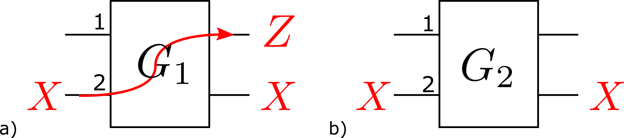
Figure 2: a): A pre-existing Pauli $X$ error on qubit 2 before some two-qubit gate $G_{1}$ remains on qubit 2, but introduces a ”new” error on qubit 1 because of the way such error propagates through $G_{1}$. What is shown graphically here is simply the equality: $Z_{1}X_{2}=G_{1}X_{2}G_{1}^{\dagger}$. b) In some cases, the $X$ errors do not propagate and stay on the same qubit, as shown here. Concrete examples of how errors propagate through different gates are shown in Figure 3.

.

Because for the Hadamard test, the measured qubit only interacts with other qubits under controlled-unitary operations (the measured qubit being on the control side), and because the measured qubit is the one that has to be isolated from the noise, we focus our interest on the conditions in which $X$ errors do not propagate from the target to the control side of the unitary. We call $c_{P}U$ a coherently controlled unitary $U$ applied if the control qubit is the eigenstate $-1$ of the single-qubit matrix $P\equiv\boldsymbol{n}.\boldsymbol{\sigma}$, where $\mathbf{n}$ is a unit vector, and $\boldsymbol{\sigma}=(X,Y,Z)$. The first thing we can easily notice is that $U$ must commute with any element in $\mathbb{P}_{n}^{X}$. Otherwise, for some state $\ket{\psi}$, for some $P_{X}\in\mathbb{P}_{n}^{X}$, we would have:

$$\bra{\psi}P_{X}^{\dagger}UP_{X}\ket{\psi}\neq\bra{\psi}U\ket{\psi}$$ (9)

It would imply that there would exist a Hadamard test, implemented on the unitary $U$ and a state $\ket{\psi}$ that would be sensitive to $X$-errors occuring in the data register. Hence, $X$-errors would propagate from the data to the measured register. This remark can be summarized as follow:

Property 3 (Necessary conditions on $U$ such that $c_{P}U$ does not propagate errors from the target to the control).

If the controlled unitary $c_{P}U$ acting on $1+n$ qubits, defined as:

$$c_{P}U\equiv\frac{1}{2}(I+P)\otimes I+\frac{1}{2}(I-P)\otimes U,$$ (10)

does not propagate $X$ errors from the target to the control, then $U$ commutes with any element in $\mathbb{P}_{n}^{X}$, which implies $U\in\mathbb{U}_{n}^{X}$.

Here, $P\equiv\mathbf{n}.\boldsymbol{\sigma}$, where $\mathbf{n}$ is a unit vector, and $\boldsymbol{\sigma}=(X,Y,Z)$. The absence of propagation of $X$-errors from the target to the control is defined as:

$$\forall P_{X}\in\mathbb{P}_{n}^{X},(c_{P}U)(I\otimes P_{X})(c_{P}U)^{\dagger}=I\otimes B$$ (11)

for some unitary $B$.

What we need to know is whether or not there are additional constraints on $U$ than being in $\mathbb{U}_{n}^{X}$. It is the case, depending on the choice of $P$. Here, we give the definition of a controlled-unitary between the measured and data register which is allowed in the computation: it shouldn’t propagate $X$-errors from the target to the control, and it should also preserve the noise bias.

Definition 4 (Bias-preserving controlled unitaries avoiding $X$-errors to propagate toward the control).

We say that the controlled-unitary

$$c_{P}U\equiv\frac{1}{2}(I+P)\otimes I+\frac{1}{2}(I-P)\otimes U$$

acting on $1+n$ qubits is bias preserving, and does not propagate $X$-errors to the control, if it satisfies

$$\forall P_{X}\in\mathbb{P}_{n+1}^{X},(c_{P}U)P_{X}(c_{P}U)^{\dagger}\in\mathbb{U}_{n}^{X}$$ (12)

$$\forall P_{X}\in\mathbb{P}_{n}^{X},\exists U_{X}\in\mathbb{U}_{n}^{X}\text{ such that,}$$

$$(c_{P}U)\left(I\otimes P_{X}\right)(c_{P}U)^{\dagger}=(I\otimes U_{X}),$$ (13)

The following property characterises the controlled unitaries between the measured and data register which are allowed in the computation (hence the ones which do not propagate $X$-errors from target to control, and preserve the noise bias).

Property 4 (Characterisation of controlled unitaries avoiding errors to propagate toward the control).

The controlled unitary $c_{X}U$ is biased preserving and avoids $X$ errors to propagate toward the control if and only if $U\in\mathbb{U}_{n}^{X}$.

The controlled unitary $c_{P}U$ with $P=yY+zZ$ is biased preserving and avoids $X$ errors to propagate toward the control if and only if $U\in\mathbb{U}_{n}^{X}$ and $U$ is Hermitian.

There doesn’t exist any controlled unitary $c_{P}U$ with any other $P=\boldsymbol{n}.\boldsymbol{\sigma}$ than previously discussed (where $\mathbf{n}$ is a unit vector, and $\boldsymbol{\sigma}=(X,Y,Z)$) that is not trivial (i.e. $U\neq I$) and that will satisfy the constraints on error propagation.

Proof.

Now, we show Property 4. We need $c_{P}U$ to satisfy the conditions (12) and (13). We begin with (13):

$$c_{P}U(I\otimes P_{X})(c_{P}U)^{\dagger}=I\otimes U_{X}$$ (14)

for some $U_{X}\in\mathbb{U}_{n}^{X}$ and for any $P_{X}\in\mathbb{P}_{n}^{X}$. This equation implies:

$$(I+\boldsymbol{n}\cdot\boldsymbol{\sigma})\otimes P_{X}+(I-\boldsymbol{n}\cdot\boldsymbol{\sigma})\otimes UP_{X}U^{\dagger}=2I\otimes U_{X}.$$ (15)

Expanding it in the Pauli basis and identifying the left and right hand sides, (15) implies that for any $P_{X}\in\mathbb{P}_{n}^{X}$, $P_{X}=UP_{X}U^{\dagger}$ and $P_{X}+UP_{X}U^{\dagger}=2U_{X}$. These equations are not independent and the first one implies the second one. As we already know that $U\in\mathbb{U}_{n}^{X}$ (see property 3), we realize that no additional constraints on $U$ (rather than $U\in\mathbb{U}_{n}^{X}$) are found here. Hence, we move on with the condition (12).

The condition (12) implies that for all $P_{X}\in\mathbb{P}_{n}^{X}$, $(c_{P}U)I\otimes P_{X}(c_{P}U)^{\dagger}\in\mathbb{U}_{n+1}^{X}$ and $(c_{P}U)X\otimes P_{X}(c_{P}U)^{\dagger}\in\mathbb{U}_{n+1}^{X}$. The first condition is already implied by (13) that we just analyzed, hence we focus on the second one. By considering $\boldsymbol{n}=(x,y,z)$, and using the fact $x^{2}+y^{2}+z^{2}=1$, we find that $(c_{P}U)X\otimes P_{X}(c_{P}U)^{\dagger}\in\mathbb{U}_{n+1}^{X}$ implies:

$$\frac{x}{2}I\otimes\big{(}P_{X}-UP_{X}U^{\dagger}\big{)}$$

$$+\frac{1}{2}X\otimes\big{(}x^{2}(P_{X}+UP_{X}U^{\dagger})+(y^{2}+z^{2})(P_{X}U^{\dagger}+UP_{X})\big{)}$$

$$+\frac{1}{2}Y^{\prime}\otimes\big{(}UP_{X}-P_{X}U^{\dagger}\big{)}$$

$$+\frac{1}{2}Z^{\prime}\otimes\big{(}P_{X}-P_{X}U^{\dagger}-UP_{X}+UP_{X}U^{\dagger}\big{)}\in\mathbb{U}_{n+1}^{X}.$$ (16)

where $Y^{\prime}\equiv iyZ-izY$ and $Z^{\prime}=x(yY+zZ)$. One can easily check that the matrices in the set $\{I,X,Y^{\prime},Z^{\prime}\}$ form a basis for the space of $2\times 2$ complex matrices. From this equation, knowing that $U\in\mathbb{U}_{n}^{X}$, the only non-trivial implications are:

$$Y^{\prime}\otimes\big{(}UP_{X}-P_{X}U^{\dagger}\big{)}=0$$ (17)

$$Z^{\prime}\otimes\big{(}P_{X}-P_{X}U^{\dagger}-UP_{X}+UP_{X}U^{\dagger}\big{)}=0$$ (18)

First case: either $y\neq 0$ or $z\neq 0$:
Knowing that $U\in\mathbb{U}_{n}^{X}$, (17) implies $U=U^{\dagger}$. Then, (18) implies that we must either have $x(yY+zZ)=0$, or $P_{X}-P_{X}U^{\dagger}-UP_{X}+UP_{X}U^{\dagger}=0$. If $P_{X}-P_{X}U^{\dagger}-UP_{X}+UP_{X}U^{\dagger}=0$ using the fact that $U$ is Hermitian and belongs to $\mathbb{U}_{n}^{X}$, the only solution for $U$ is $U=I$ which is a trivial gate. Hence, in order to find non-trivial gates, we must have $x=0$. In conclusion, if $y\neq 0$ or $z\neq 0$ then necessarily $U$ is Hermitian and $x=0$ in order to satisfy the constraints (17), (18) with $U\neq I$.
Second case: $y=z=0\Leftrightarrow x=1$:
In such a case, there are no additional constraints: any $U\in\mathbb{U}_{n}^{X}$ will satisfy the constraints (17), (18).

Here, we provided necessary conditions on $U$, $(x,y,z)$ but one could check that injecting any of the solutions would satisfy the constraints. Hence our conditions are necessary and sufficient. ∎

A.3 Example of bias-preserving gates

Here, we provide concrete examples of bias-preserving gates and we show how they propagate errors in circuits. It is worth noticing that while bias-preserving gates do exist ”in principle”, being able to actually implement them in a bias-preserving manner is not straightforward in general. This is because, in the laboratory, these gates are implemented through continuous Hamiltonian evolution. If the Hamiltonian used to perform the gate contains Pauli $Z$-terms, it might be that a bit-flip ($X$-error) produced during the gate evolution will be converted to a phase flip ($Z$-error). For instance, while a cNOT preserves $X$-errors ”in principle”, it is not straightforward to guarantee that this condition still holds if we consider a continuous-time evolution to implement the gate. In practice, this issue can be resolved with cat-qubits [45], and both the $\text{Toffoli'}\equiv H_{1}H_{2}H_{3}\times\text{Toffoli}\times(H_{1}H_{2}H_{3})^{\dagger}$ and cNOT can be shown to preserve $X$-errors [46, 45]. Here, we recall that in our work we took a different convention for the dominant source of errors (in [46, 45] they consider that the main source of errors are phase-flips, i.e. $Z$ errors while we consider bit-flips, i.e. $X$ errors). Hence we ”convert” their results to our convention simply by ”swapping” the role of $X$ and $Z$ for the gate definitions. This is why we can say that Toffoli’ and cNOT preserve the bit-flip bias.

The propagation of errors through cNOT and Toffoli’ is shown in figure 3. There, we see that depending on which qubit had a pre-existing Pauli $X$ error, this error can propagate toward multiple qubit. Sometimes, the resulting error is no longer a Pauli operator as shown in figure 3 b). However, because we consider bias-preserving gates, we are guaranteed that for pre-existing Pauli-X errors, the resulting error after the gate is an element of $\mathbb{U}_{n}^{X}$. In this figure, we also showed how $Z$ errors would propagate through a cNOT (the definitions provided in the main text can naturally be generalized to $Y$ and $Z$ operators). The propagation for $Y$ errors can be deduced from the propagation of $Y$ and $Z$ errors. Toffoli’ does not preserve $Z$ errors (a pre-existing $Z$ error on any of the control would not be anymore a $Z$ error after the gate).

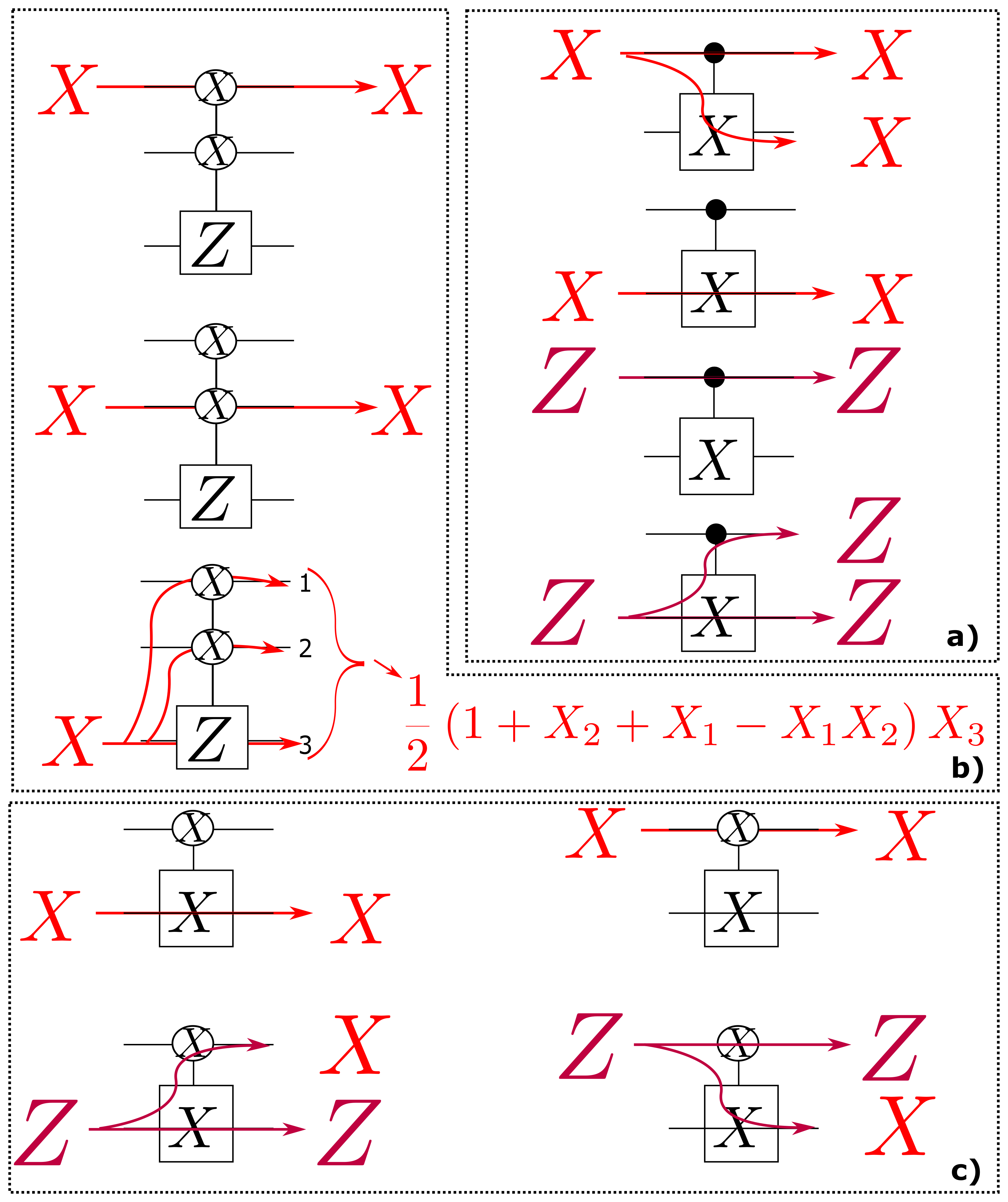
Figure 3: On this image, we represent how some initial Pauli errors ($X$ or $Z$) propagate through different bias-preserving gates. In particular, we give examples of bias-preserving gates (preserving $X$-errors) with a cNOT, Toffoli’ (we call Toffoli’ a Toffoli where the role of $X$ and $Z$ have been exchanged), and $c_{X}X$ ($c_{X}G$ means the application of a gate $G$ coherently controlled in the $X$ basis, i.e., applied for the control being in $\ket{-}$ and not applied if the control is in $\ket{+}$). Coherent control in the $X$ basis is represented by an $X$ inside of a black circle (visible on the top qubit on c) for instance). On a), we see that an $X$ error in a cNOT propagates from the control to the target, but not the other way around. A $Z$ error propagates from the target to the control, but never from the control to the target. On b), we see that a Toffoli’ propagates $X$-errors toward multiple qubits only in the case a pre-existing error on the target qubit occurred. In such a case, the resulting error is no longer an element of $\mathbb{P}_{n}^{X}$, but it belongs to $\mathbb{U}_{n}^{X}$. Toffoli’ would not preserve $Z$ (or $Y$) errors. On c), we see that an $X$ error trivially commutes with $c_{X}X$. For such a gate, the $Z$ errors are not preserved: a Pauli $Z$ before $c_{X}X$ would be equivalent to $c_{X}X$ followed by an operator that is no longer a Pauli $Z$ operator as shown in the two examples at the bottom.

Appendix B Properties of the preparable states $\ket{\psi}$

B.1 Diagonal unitaries in $X$ basis for the preparation are unnecessary

Property 5.

We consider the preparation unitary of the Hadamard test, $B$, to be a product of bias-preserving gates. Any gate in $\mathbb{U}_{n}^{X}$, used inside the unitary $B$ cannot change the expectation value $\bra{\psi}U\ket{\psi}$ for $U\in\mathbb{U}_{n}^{X}$.

Proof.

In order to show this property, we will first assume that $B=C\times B^{\prime}$, where $C\in\mathbb{U}_{n}^{X}$. We then have:

$$\ket{\psi}\equiv C\ket{\Psi}=CB^{\prime}\bigotimes_{i=1}^{n}\ket{\phi_{i}},$$ (19)

where the family $\{\ket{\phi_{i}}\}_{i=1}^{n}$ represents the initial single qubit states prepared in the data register. In such a case, we have:

$$\bra{\psi}U\ket{\psi}=\bra{\Psi}C^{\dagger}UC\ket{\Psi}=\bra{\Psi}U\ket{\Psi},$$ (20)

where we used the fact that $[C,U]=0$ for the last equality (because $(C,U)\in\mathbb{U}_{n}^{X}$). Hence, it shows that there is no interest in applying a unitary $C\in\mathbb{U}_{n}^{X}$ right before the controlled $U$ as it won’t have any influence on the expectation value. It remains to understand what happens if $C$ was applied before this point. Let’s assume for instance that $B=B_{1}CB_{2}$, where $C\in\mathbb{U}_{n}^{X}$. Using the fact that all the gates used in $B$ belong to $\mathbb{B}_{n}$, $B_{1}$ is also in $\mathbb{B}_{n}$. Hence, $B_{1}C=C^{\prime}B_{1}$, with $C^{\prime}\in\mathbb{U}_{n}^{X}$. As shown above, $C^{\prime}$ cannot change the expectation value $\bra{\psi}U\ket{\psi}$. Hence, it means that implementing $B=B_{1}CB_{2}$, or implementing instead $B_{1}B_{2}$ would lead to the same result. Overall, we showed that any gate $C\in\mathbb{U}_{n}^{X}$ used in the preparation unitary $B$ can be removed as it doesn’t change the expectation value for the Hadamard test. ∎

Alternatively, Property 5 also implies that all the single qubit states $\ket{\phi_{i}}$ that differ by a rotation around the $X$-axis of the Bloch sphere would lead to the same expectation value (for instance initializing $\ket{\phi_{i}}$ in an eigenstate of $Y$ or $Z$ would provide the same outcome for the Hadamard test).

B.2 Additional remarks about entanglement properties

Here, we wish to comment on different properties about the kind of entanglement that can be generated with bias-preserving circuits, and how they are used in our specific examples based on the Hadamard test. In the discussion part of the main text, we explained that highly entangled graph states can be generated. This is done by initializing the data register in $\ket{0}^{\otimes n}$, and applying some gates $c_{X}X\in\mathbb{U}_{n}^{X}$ in the preparation unitary $B$. It shows that in general bias-preserving circuit can generate quantum states having interesting computational properties, a remark worth noticing for possible extensions of our work.

However, it should be noticed that in the specific computational task we addressed in our study, namely, performing a restrictive class of Hadamard tests, the Property 5 indicates that these $c_{X}X$ gates will not modify the measurement outcomes. Hence, it means that bias-preserving circuits can be used to prepare these highly entangled graph states, but for our specific task, they would provide the same outcome as an Hadamard test being $\bra{0^{\otimes n}}U\ket{0^{\otimes n}}$, for any $U$ allowed by Theorem 1. It might be worth to notice that $U$ itself can be an entangling operation here.

This is however not an issue for our goals: (i) it does not rule out the interest of the benchmarking protocol on these states, and (ii) we can prepare other entangled states for which the entangling operations used in their preparation play a role in the result of the Hadamard test. For (i), the purpose of the verification is to check whether or not the circuit used to prepare these highly entangled states works as expected. In the absence of any errors, our example simply means that the expectation value for this Hadamard test is the same as the one obtained for $\ket{\psi}=\ket{0}^{\otimes n}$. In the presence of an imperfect bias, even though the preparation unitary $B$ is solely composed of $c_{X}X$ gates, the circuit will (in general) propagate $Y$ and $Z$ errors to the measured register, significantly modifying its density matrix compared to the noiseless case. Hence, the verification protocol would still allow to verify whether or not the highly entangled states have been prepared in a bias-preserving manner, i.e. in a manner that they are only affected by $X$-errors. This verification is possible for the unitaries allowed by Theorem 1 (we would also need to have $\bra{0^{\otimes n}}U\ket{0^{\otimes n}}\neq 0$, a condition that can be met in our case).

For (ii), it is easy to create entangled states for which the gates used to create this entanglement will play a role in the expectation value of the Hadamard test. A simple example can be an $n$-qubit GHZ state. It can be created by initializing the first qubit in $\ket{+}$, the rest of the qubits in $\ket{0}^{\otimes{n-1}}$ and by applying a sequence of cNOTs controlled by the first qubit (targetted on the rest of the qubits). While belonging to $\mathbb{B}_{n}^{X}$, the cNOTs do not belong to $\mathbb{U}_{n}^{X}$. Because of that, the preparation unitary $B$ itself will have an influence on the measured outcome. Overall an exact characterisation of all entangled states that can be created in our circuits goes beyond the scope of this paper.

Appendix C Proof of the main results

C.1 Preliminary result

Property 1 (Preservation of the bias).

If a quantum circuit is only composed of gates in $\mathbb{B}_{n}$, each subject to the local biased noise model (2) of the main text (and the paragraph that follows for measurement and preparation), then any error affecting the state of the computation is an $X$-error (this property can be generalized ”by linearity” for a perfect bias, not necessarily Pauli according to definition 5: we use this fact in the proof of theorem 3).

Proof.

After initialization, in the absence of errors, the state of the computation would be $\ket{\psi_{\text{prep}}}=\bigotimes_{i=1}^{n}\ket{\phi_{i}}$. Because the initialization is noisy, following the noise model described around (2) (of the main text), the state after preparation will be in some mixture:

$$\rho_{i}=\sum_{\alpha}p^{\text{prep}}_{\alpha}X_{\alpha}{|\psi_{\text{prep}}\rangle\langle\psi_{\text{prep}}|}X_{\alpha}^{\dagger}$$ (21)

for some probabilities $p^{\text{prep}}_{\alpha}$. In this equation (and the equations that follow), the sum over $\alpha$ is such that all $n$-qubit Pauli-$X$ operator will be reached exactly once, for some $X_{\alpha}$ (more formally, the sum is such that $\alpha\subset\mathrm{supp}(I_{n})$ for $I_{n}$ an identity matrix applied on $n$ qubits). We now consider a gate $G\in\mathbb{B}_{n}$. For any state $\ket{\Psi}$, we have, for some probability $p^{G}_{\alpha}$:

$$\mathcal{E}({|\Psi\rangle\langle\Psi|}) =\mathcal{N}_{\mathcal{G}}\circ\mathcal{G}({|\Psi\rangle\langle\Psi|})$$

$$=\sum_{\alpha}p^{G}_{\alpha}X_{\alpha}G{|\Psi\rangle\langle\Psi|}G^{\dagger}X_{\alpha}^{\dagger}$$ (22)

Hence, we have:

$$\mathcal{E}(\rho_{i})=\sum_{\alpha_{1},\alpha_{2}}p^{G}_{\alpha_{1}}p^{\text{prep}}_{\alpha_{2}}X_{\alpha_{1}}GX_{\alpha_{2}}{|\psi_{\text{prep}}\rangle\langle\psi_{\text{prep}}|}X_{\alpha_{2}}^{\dagger}G^{\dagger}X_{\alpha_{1}}^{\dagger}$$ (23)

Using the fact $G\in\mathbb{B}_{n}$, we have: $GX_{\alpha_{2}}=E_{\alpha_{2}}G$ for some $E_{\alpha_{2}}\in\mathbb{U}_{n}^{X}$. Hence:

$$\mathcal{E}(\rho_{i})=\sum_{\alpha_{1},\alpha_{2}}p^{G}_{\alpha_{1}}p^{\text{prep}}_{\alpha_{2}}X_{\alpha_{1}}E_{\alpha_{2}}G{|\psi_{\text{prep}}\rangle\langle\psi_{\text{prep}}|}G^{\dagger}E_{\alpha_{2}}^{\dagger}X_{\alpha_{1}}^{\dagger}$$ (24)

Because $X_{\alpha_{1}}\times E_{\alpha_{2}}\in\mathbb{U}_{n}^{X}$, it shows that the noiseless and noisy state of the computation (after noisy preparation and noisy gate $G$) only differ through the presence of errors in $\mathbb{U}_{n}^{X}$. The same reasoning could be applied recursively for any gate applied after this point, showing that the property 1 is true. ∎

C.2 Proof of Theorem I of the main text (with noiseless identity gates)

Theorem 1 (Hadamard test resilient to biased noise).

Let:

$$\ket{\psi}=B\bigotimes_{i=1}^{N_{B}}\ket{\phi_{i}},\ U=W\cdot V\ ,$$

$$\ W\equiv\prod_{i=1}^{N_{W}}W_{i},\ V\equiv\prod_{i=1}^{N_{V}}V_{i}\ ,$$ (25)

where $B$ is a product of local bias preserving gates, gates $V_{i}$ and $W_{i}$ are local gates and belong to $\mathbb{U}_{n}^{X}$. Additionally, the gates $W_{i}$ are assumed to be Hermitian.

Furthermore, we assume the local bias noise model introduced in Eq. (2) (of the main text), and that state preparation, measurements, and each non-trivial gate applied on the measurement register have a probability at most $p<1/2$ to introduce a bit-flip on the measured register.

Under these conditions, there exists a quantum circuit realising a Hadamard test such that, in the presence of noise, the reduced state $\rho$ satisfies

$$\rho=\frac{1}{2}\left(I+\alpha_{n}\left(yY+zZ\right)\right)\,$$ (26)

with $\alpha_{n}\geq(1-2p)^{O(N_{V})}$.

Additionally, $\alpha_{n}$ is efficiently computable classically. Hence, if $N_{V}=O(\log(n))$, it is possible to implement the Hadamard test in such a way that running the algorithm $\text{poly}(n)$ times is sufficient to estimate the real and imaginary parts of $\bra{\psi}U\ket{\psi}$ to $\epsilon$ precision with high probability.

Proof.

We focus our interest on figure 4. In this image, the controlled unitaries with a blue contour correspond to the $W_{i}$, and the ones with a black contour to the $V_{i}$. We first explain how the $U$ defined in Theorem 1 is implemented. Then we will show that the circuit is noise-resilient. Attributing the indices $m,p,d$ for, respectively, the measured, parallelisation and data registers, and calling $q_{n}\leq n$ the number of qubits in the parallelisation register, the full state of the computer right before the application of any controlled $W_{i}$ or $V_{i}$ is the entangled state:

$$\ket{\Psi}_{0}\equiv\frac{\ket{+}_{m}\ket{0}^{\otimes q_{n}}_{p}+\ket{-}_{m}\ket{1}^{\otimes q_{n}}_{p}}{\sqrt{2}}\otimes\ket{\psi}_{d}.$$ (27)

This entanglement has been created thanks to a sequence of cNOT and $c_{X}X$ gates (see Figure 4). Now, we apply the controlled $W_{i}$ and the state becomes:

$$\ket{\Psi}_{0}\to$$

$$\frac{\ket{+}_{m}\ket{0}^{\otimes q_{n}}_{p}\ket{\psi}_{d}+\ket{-}_{m}\ket{1}^{\otimes q_{n}}_{p}\prod_{i=1}^{N_{W}}W_{i}\ket{\psi}_{d}}{\sqrt{2}}.$$ (28)

The parallelisation register is then decoupled from the rest (by applying the reverse sequence of cNOT and $c_{X}X$). Discarding this state, and applying the last sequence of coherently controlled $V_{i}$, we get the required final state for the Hadamard test:

$$\ket{\Psi}_{f}=\frac{\ket{+}_{m}\ket{\psi}_{d}+\ket{-}_{m}U\ket{\psi}_{d}}{\sqrt{2}},$$ (29)

where

$$U=\prod_{i=1}^{N_{W}}W_{i}\times\prod_{i=1}^{N_{V}}V_{i}.$$ (30)

It proves that the appropriate operation is implemented. The parallelisation gadget we use is based on [64].

Now, we need to show that this circuit is noise-resilient. We call $p_{i}$ the probability that the $i$’th gate applied on the measured register introduces a bit-flip error there. For a multi-qubit gate $\mathcal{G}_{i}$, considering that the measured register is the first qubit in the tensor decomposition, this probability is defined as:

$$p_{i}\equiv\sum_{\begin{subarray}{c}(1,\alpha^{\prime})\subset\mathrm{supp}(\mathcal{G}_{i})\end{subarray}}p^{\mathcal{G}_{i}}_{1,\alpha^{\prime}}$$ (31)

To clarify the notation with an example, it means that for a two-qubit gate having the noise model:

$$\mathcal{N}(\rho)=\sum_{\begin{subarray}{c}0\leq i_{1}\leq 1\\ 0\leq i_{2}\leq 1\end{subarray}}p_{i_{1},i_{2}}(\sigma_{i_{1}}\otimes\sigma_{i_{2}})\rho(\sigma_{i_{1}}\otimes\sigma_{i_{2}}),$$ (32)

the probability to introduce a bit-flip on the measured register (first tensor product) would be $\sum_{0\leq i_{2}\leq 1}p_{1,i_{2}}$. In what follows we will also include noisy state preparation and measurements in the derivation.

We first notice only $X$-errors can occur in the whole algorithm. This is because we use the noise model described around (2) (of the main text), and all our gates are bias-preserving (see properties 1 and 4). We also notice from this last property that the reason why the $W_{i}$ must be Hermitian is that they are coherently controlled on the $Z$ basis. At this point, we can additionally notice that all the gates interacting with the measured register cannot propagate $X$-error from neither the parallelisation nor the data register toward the measured register: this is another consequence of property 4. We should emphasize on this last point: the fact we trade space for time with the parallelisation register (it introduces additional qubits in the algorithm, but it allows the measured register to interact with $O(N_{V})=O(\log(n))$ and not $O(N_{W})\subset\text{poly}(n)$ gates) is what allows us to guarantee the noise-resilience of our circuit. The key point in this trade is that the errors produced on the parallelisation register cannot propagate to the measured one, because they commute with the only gate interacting with the measured register: $c_{X}X$. Without the use of this parallelisation register, the measured register would face errors at $O(N_{W})$ additional locations, ruining the scalability for $N_{W}=\text{poly}(n)$. Our remarks here still hold (with one additional hypothesis), considering waiting location (identity gates) to be noisy, as discussed in the following section. Overall, here we showed that all the errors that can damage the measurements are ”directly” produced on the measured register.

Here comes the last part of the proof: now that we know that everything behaves ”as if” the only noisy qubit was the measured one, we need to compute the effect of this noise. After the $i$’th gate interacts with the measured register, the following bit-flip channel is applied on the measured register, for some $p_{i}$ (and $\sigma$ is some density matrix):

$$\Lambda_{i}(\sigma)=(1-p_{i})\sigma+p_{i}X\sigma X.$$ (33)

This noise model naturally includes the noise produced after state preparation. We can also model noisy measurements with this noise channel. This is because they are modelled as perfect ones followed by a probability to flip the measured outcome. Because we measure Pauli $Y$ and $Z$, we can equivalently model them as perfect measurements preceded with a bit-flip channel.

Now, we use the fact the bit-flip channel commutes with every gate applied on the measured register (they are coherently controlled in the $X$-basis). Hence, calling $N_{n}$ the number of gates applied on the measured register (including state preparation and measurement), the full protocol is equivalent as performing noiseless measurements in $Y$ or $Z$ bases on the state:

$$\rho=(\Lambda_{N_{n}}\circ...\circ\Lambda_{1})(\rho_{\text{ideal}}),$$ (34)

$$\rho_{\text{ideal}}=\frac{1}{2}(I+yY+zZ).$$ (35)

It is straightforward to show that:

$$\rho=\frac{1}{2}(I+\alpha_{n}(yY+zZ)),$$

$$\alpha_{n}=\prod_{i=1}^{N_{n}}(1-2p_{i}).$$ (36)

In the case identity gates are noiseless, we have $N_{n}=N_{V}+2+2=O(N_{V})$. The first ”$+2$” corresponds to state preparation and measurement, and the last one to the implementation of the $c_{X}X$ gates with the parallelisation register, as shown on Figure 4. We discuss what happens if identity gates are noisy in the following section. We notice that $\alpha_{n}$ is efficiently computable classically (as long as $N_{n}\in\text{poly}(n)$). Calling $p=\max_{i}p_{i}$, it is easy to see that $\alpha_{n}\geq(1-2p)^{O(N_{V})}$ is true. Hence, if $N_{V}=O(\log(n))$, $\alpha_{n}$ decreases at a polynomial speed at most and is efficiently computable. Following the explanations after Eq. (1) in the main text, it implies that it is possible to implement the Hadamard test in such a way that running the algorithm $\text{poly}(n)$ times is sufficient to estimate the real and imaginary parts of $\bra{\psi}U\ket{\psi}$ to $\epsilon$ precision with a probability greater than $1-\delta$. ∎

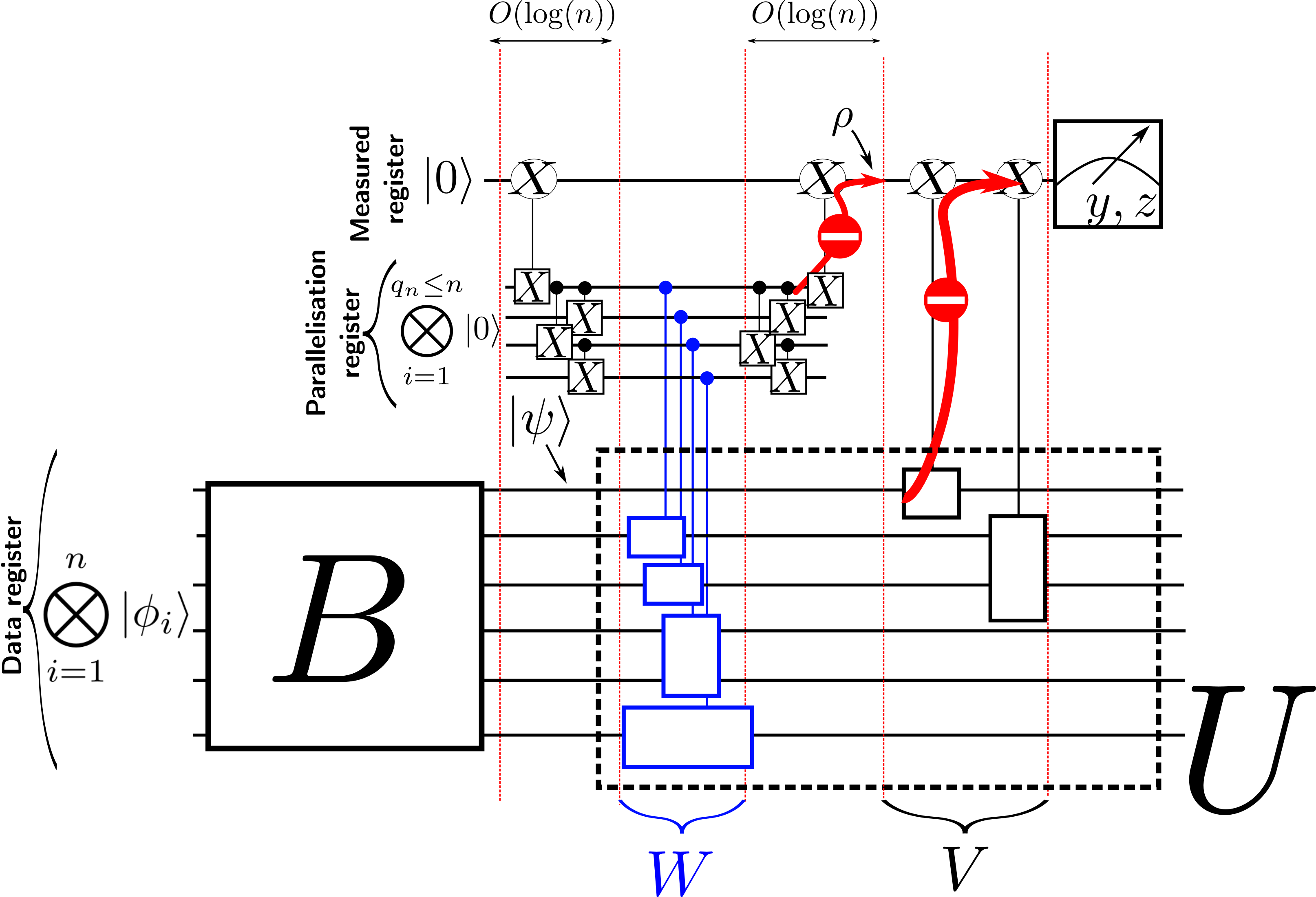
Figure 4: In this figure, we illustrate how $U=W\times V=\bigotimes_{i=1}^{N_{W}}W_{i}\times\bigotimes_{i=1}^{N_{V}}V_{i}$ can be implemented in a noise-resilient manner. The coherently controlled unitaries with a blue contour correspond to the Hermitian unitaries $W_{i}$ (implementing $W$), and the coherently controlled unitaries with a black contour correspond to $V_{i}$ (implementing $V$). The central element in this construction is the parallelisation register [64], which allows to implement a unitary $U$ that interacts with all the qubits in the data register while preserving the noise-resilience. The key point behind the parallelisation register is that, while it introduces additional components that can introduce errors, these errors cannot, by construction, propagate to the measured register (in practice, they commute with the second $c_{X}X$ gate represented). It is an example where trading space (using more qubits) to gain time (guaranteeing that the measured register interacts with $O(\log(n))$ gates and not $\text{poly}(n)$ gates) is worth doing.

C.3 Extension of Theorem 1 for noisy identity gates

In the assumption of Theorem 1, any trivial (i.e. identity) gate applied on the measured register was assumed to be noiseless. However, the use of the parallelisation register may introduce a significant number of ”waiting” locations for the measured qubit (at least for the initialization of the parallelisation register, or for the implementation of $W$). Fortunately, assuming that the depth of $W$ is in $O(\log(n))$, we could include noisy identity gates in the reasonning while not changing any of our conclusions. To keep the explanation simple, we assume that all gates in the computation (including identity) last for the same amount of time. We call $p_{I}$ the probability that an identity gate introduces a bit-flip, and we call $N_{I}$ the number of identity gates applied on the measured register. In such a case, the only thing that would change in the proof of Theorem 1 would be that:

$$\alpha_{n}=(1-2p_{I})^{N_{I}}\prod_{i=1}^{N_{n}}(1-2p_{i}).$$ (37)

There, $\prod_{i=1}^{N_{n}}(1-2p_{i})$ is the probability that the non-trivial gates (including preparation and measurements) introduce bit-flips. The new term $(1-2p_{I})^{N_{I}}$ corresponds to the noise introduced by identity gates. In the case $W$ has a depth in $O(\log(n))$, we could implement the algorithm with $N_{I}=O(\log(n))$ (see figure 4): the algorithm would still be noise-resilient. It would be the case as $\alpha_{n}$ would decrease at polynomial speed while being exactly computable. If the depth of $W$ is not in $O(\log(n))$, the identity gates might lead to an exponential decay of $\alpha_{n}$, ruining the scalability. It would for instance be the case if the depth of $W$ is linear in $n$ (in this case, $N_{I}\propto n$). One key element in this discussion is that the entanglement (and dis-entanglement) between the measured and parallelisation register can be done in $O(\log(n))$ depth [64], as also illustrated on the figure 4.

In conclusion, if the depth of $W$ is in $O(\log(n))$, then the main conclusion behind theorem 1 (the fact running the algorithm $\text{poly}(n)$ times is sufficient to estimate the real and imaginary parts of $\bra{\psi}U\ket{\psi}$ to $\epsilon$-precision with high probability) would also hold with noisy identity gates.

C.4 Efficient classical simulation

Theorem 2 (Efficient classical simulation of restricted Hadamard test).

Let $B\in\mathbb{B}_{n},U\in\mathbb{U}^{X}_{n}$ be n qubit unitaries specified by $R_{B}$ and $R_{U}$ local qubit gates (belonging to respective classes $\mathbb{B}_{n}$ and $\mathbb{U}^{X}_{n}$). Let $\ket{\psi_{0}}=\ket{\phi_{1}}\ket{\phi_{2}}\cdots\ket{\phi_{n}}$ be an initial product state. Then, there exists a randomized classical algorithm $\mathcal{C}$, taking as input classical specifications of circuits defining $B$, $U$, and the initial state $\ket{\psi_{0}}$, that efficiently and with a high probability computes an additive approximation to $\bra{\psi_{0}}B^{\dagger}UB\ket{\psi_{0}}$. Specifically, we have

$$\Pr\left(|\bra{\psi_{0}}B^{\dagger}UB\ket{\psi_{0}}-\mathcal{C}|\leq\epsilon\right)\geq 1-\delta\ ,$$ (38)

while the running time is $T=O\left(\frac{R_{B}+R_{U}+n}{\epsilon^{2}}\log(1/\delta)\right)$.

Proof.

We first note that $B^{\dagger}UB\in\mathbb{U}_{n}^{X}$ is diagonal in the local $X$ basis. For this reason we can rewrite

$$\bra{\psi_{0}}B^{\dagger}UB\ket{\psi_{0}}=\Tr\left(B^{\dagger}UB\ \rho_{1}\otimes\rho_{2}\otimes\ldots\otimes\rho_{n}\right)\ ,$$ (39)

where the $\rho_{i}$ are states acting on the i’th qubit and defined as the : $\rho_{i}=\frac{1}{2}{|\phi_{i}\rangle\langle\phi_{i}|}+\frac{1}{2}X{|\phi_{i}\rangle\langle\phi_{i}|}X$ (dephased version of $\ket{\psi_{i}}$ in the $X$ basis). We can rewrite each $\rho_{i}$ as: $\rho_{i}=p^{+}_{i}{|+\rangle\langle+|}+p^{-}_{i}{|-\rangle\langle-|}$, where the computation of the all the probabilities $p_{i}^{\pm}$ can be done in $O(n)$ time. Equation (39) and the structure of unitaries $B,U$ can be used to derive an efficient sampling procedure for estimating $\bra{\psi_{0}}B^{\dagger}UB\ket{\psi_{0}}$. To this end, we decompose

$$\rho_{1}\otimes\rho_{2}\otimes\ldots\otimes\rho_{n}=\sum_{\mathbf{s}\in\{+,-\}^{n}}p_{\mathbf{s}}{|\mathbf{s}\rangle\langle\mathbf{s}|}\,$$ (40)

where $p_{\mathbf{s}}=\prod_{i=1}^{n}p_{i}^{s_{i}}$ is a product distribution. Inserting (40) into right-hand side of (39) we obtain

$$\bra{\psi_{0}}B^{\dagger}UB\ket{\psi_{0}}=\sum_{\mathbf{s}\in\{+,-\}^{n}}p_{\mathbf{s}}\Tr\left(UB{|\mathbf{s}\rangle\langle\mathbf{s}|}B^{\dagger}\right)\ .$$ (41)

The above formula can be simplified further by realising that $B{|\mathbf{s}\rangle\langle\mathbf{s}|}B^{\dagger}={|\sigma_{B}(\mathbf{s})\rangle\langle\sigma_{B}(\mathbf{s})|}$ (cf. Property 2) and by utilising $U\in\mathbb{U}^{X}_{n}$ (which implies $U\ket{\mathbf{s}}=\lambda_{U}(\mathbf{s})\ket{\mathbf{s}}$, for all $\ket{\mathbf{s}}$). Putting this all together we obtain

$$\bra{\psi_{0}}B^{\dagger}UB\ket{\psi_{0}}=\sum_{\mathbf{s}\in\{+,-\}^{n}}p_{\mathbf{s}}\lambda_{U}(\sigma_{B}(\mathbf{s}))\ .$$ (42)

The above equation shows that the random variables $x_{\mathbf{s}}=\mathrm{Re}(\lambda_{U}(\sigma_{B}(\mathbf{s}))),y_{\mathbf{s}}=\mathrm{Im}(\lambda_{U}(\sigma_{B}(\mathbf{s})))$ are unbiased estimators of the real and imaginary parts of $\bra{\psi_{0}}B^{\dagger}UB\ket{\psi_{0}}$ respectively. This suggests a straightforward three steps algorithm for constructing estimators of the quantities of interests: (i) generate $\mathbf{s}\sim\{p_{\mathbf{s}}\}$, (ii) compute $\mathbf{s}^{\prime}=\sigma_{B}(\mathbf{s})$, (iii) evaluate $\lambda_{U}(\mathbf{s}^{\prime})$ in order to compute $x_{\mathbf{s}},y_{\mathbf{s}}$. From Hoeffding’s inequality (both $x_{\mathbf{s}}$ and $y_{\mathbf{s}}$ take values in the interval $[-1,1]$) it follows that repeating the above procedure $O((1/\epsilon^{2})\log(1/\delta))$ times and taking sample means gives $\epsilon$ -accurate estimation of $\bra{\psi_{0}}B^{\dagger}UB\ket{\psi_{0}}$ with probability at least $1-\delta$.

What remains to be shown is the classical computation cost of steps (i)-(iii). Since $\mathbf{s}$ is distributed according to the simple product measure on $n$ bits, generation of a single sample takes $O(n)$ time. With regards to (ii) we use Property 2 and the decomposition of $B$ into a sequence of $R_{B}$ local gates from $\mathbb{B}_{n}$ - since each gate acts locally, it will induce an easily tracktable transformation of $\ket{\mathbf{s}}$ in only a subset $\beta$ of constant size. Consequently, the overall cost of implementing (ii) is thus $O(R_{B})$. Similar argument holds for the final step (iii) - now the unitary $U$ is decomposed into a sequence of local unitaries $g_{j}$ from $\mathbb{U}^{X}_{n}$. Naturally, we have $U\ket{\mathbf{s}^{\prime}}=\prod_{j=1}^{R_{U}}\lambda_{j}(\mathbf{s}^{\prime})\ket{\mathbf{s}^{\prime}}$, where $\lambda_{j}(\mathbf{s}^{\prime})$ are defined by $g_{j}\ket{\mathbf{s}^{\prime}}=\lambda_{j}(\mathbf{s}^{\prime})\ket{\mathbf{s}^{\prime}}$. Since gates $g_{j}\in\mathbb{U}^{x}_{n}$ are local, individual eigenvalues $\lambda_{j}(\mathbf{s}^{\prime})$ can be computed in constant time and depend only on the few bit in $\mathbf{s}^{\prime}$. Overall, the cost of this step is therefore $O(R_{U})$. Combining the above estimates for runtimes of each of the steps of the protocol we get the desired result. ∎

Appendix D Additional noise resilience properties

D.1 The circuit is noise-resilient against various scale-dependent noise

Throughout this paper, we considered that the probability to introduce a bit-flip on the measured register after each gate applied on it is upper bounded by some constant probability $p<1/2$. However, in current experiments, it frequently happens that the probability of error for quantum gates grows with the number of qubits involved, hence with the problem size, $n$ [61, 65]. It can for instance happen because of crosstalk [62, 63]. More importantly, in this work we assumed the bias to be perfect, i.e. $Z$ or $Y$ errors were never produced. This is an idealization as, while being several orders of magnitudes less frequent than $X$ errors [47], $Z$ and $Y$ errors can still occur. In practice, for a biased hardware based on cat qubits, it is possible to experimentally tune the average number of photons, $\bar{n}$, contained in the cat state, such that the $Z$ and $Y$ error rates will exponentially decrease with $\bar{n}$ at the cost of a linear growth of the $X$-error rate [46]. What one could then consider is to choose a high enough $\bar{n}$ such that the probability to have either a $Z$ or $Y$ error after the (noisiest) gate $p_{Z/Y}(\bar{n})$ satisfies $p_{Z/Y}(\bar{n})N_{\text{gates}}(n)\ll 1$, where $N_{\text{gates}}(n)$ is the total number of gates used in the algorithm. It would guarantee that ”in practice”, one could safely neglect $Y$ or $Z$ errors and consider the bias to be perfect. The cost of this condition is that $\bar{n}$ has to increase with $n$, meaning that the bit-flip rate, $p$, also increases with $n$: this is another example of scale-dependent noise.

An interesting feature occurring in our circuits is that they can, to some extent, be resilient against various classes of scale-dependent noise: the polynomial overhead in the algorithm repetitions can be preserved in that case. Our goal here is to provide conditions on how the probability to introduce bit-flip after each gate applied on the measured register, $p_{n}$ (the index $n$ now represents the scale dependence) is allowed to grow with $n$ in order to see this behavior. We then give a few concrete examples.

We consider that the probability to introduce a bit-flip on the measured register is upper bounded by $p_{n}<1/2$, for any gate applied there. We assume that the probability of errors for each gate is known. The result of Theorem 1 guarantees that $\alpha_{n}\geq(1-2p_{n})^{O(N_{V})}$, with $\alpha_{n}$ efficiently computable classically. Calling $C_{n}$ a sufficient number of algorithms calls allowing to estimate $\bra{\psi}U\ket{\psi}$ up to $\epsilon$-precision with a probability $1-\delta$, we know from the main text that we can take: $C_{n}=2\log(2/\delta)/(\alpha_{n}\epsilon^{2})$. We would then have $C_{n}\leq 2\log(2/\delta)/(\epsilon(1-2p_{n})^{O(N_{V})})^{2}$. For the same reasons as explained in the main text, the scaling in $1/(\epsilon(1-2p_{n})^{O(N_{V})})^{2}$ is also optimal.

Hence, as long as $1/((1-2p_{n})^{O(N_{V})})$ grows polynomially with $n$, the scalability would be preserved. It can for instance occur if $N_{V}$ is a constant, independent on $n$ and $p_{n}=(1-\Delta_{n})/2$ for $\Delta_{n}=A/n^{k}$. (for $A,k\geq 0$). We could also imagine that both $N_{V}$ and $p_{n}$ grow with $n$. For instance, if we impose that $N_{V}=\sqrt{\log(n)}=|\log(\Delta_{n})|$, then one can easily check that it also leads to a scalable, noise-resilient algorithm.

In this discussion, we used the results of Theorem 1 which assumes noiseless identity gates. Similar results can easily be obtained in the case identity gates are noisy (see the discussion of such a case, in section C.3).

Overall, we have shown here that the algorithm we studied can also be noise resilient in presence of some scale-dependent noise, and we illustrated it with simple examples. This is an interesting property given the current limitations of the hardware in quantum computing, that can often lead to scale-dependent noise [61].

D.2 The Hadamard test is resilient against noisy-measurements

As shown in property 4, the unitary $U$ used in the Hadamard test must belong to $\mathbb{U}_{n}^{X}$. Because of that, in principle, we could simply measure the data register in the $X$ basis (and remove the measured register from the algorithm) in order to deduce $\bra{\psi}U\ket{\psi}$. In this part, we wish to show that measuring the qubits of the data register will not be scalable, as soon as the measurements are noisy and one needs to measure $\text{poly}(n)$ measurements: the measured register is in general necessary.

To show it, we only need one example of a loss of scalability for a polynomial number of measured qubits. Here, we assume that the state to be measured is guaranteed to be in some product state $\bigotimes_{i=1}^{n}\ket{\phi_{i}}$ ($\ket{\phi_{i}}\in\{\ket{+},\ket{-}\}$), unknown to the experimentalist. Its goal is to find if the state is an eigenstate $+1$ or $-1$ of the observable $X^{\otimes n}$. In order to find this out, it measures all the qubits in the $X$-basis. Unfortunately, these measurements have a probability $p_{\text{meas}}$ to be wrong (i.e. to return $-1$ while the measurement should produce $+1$, and vice-versa).

We can easily compute the probability to obtain the correct measurement outcome after a single trial: it corresponds to the probability that an even number of qubits were wrongly measured. We have:

$$p_{\text{correct}} =\sum_{i=0,i\ \text{even}}^{n}\binom{n}{i}p_{\text{meas}}^{i}(1-p_{\text{meas}})^{n-i}$$

$$=\frac{1}{2}(1+(1-2p_{\text{meas}})^{n})>1/2$$ (43)

In practice, the experimentalist will have access to estimators of $p(+1)$ and $p(-1)$: the probabilities that $X^{\otimes n}$ yields $+1$ or $-1$ as measurement outcome. Then, it needs to distinguish these two probability distributions. Calling $p(+1)$ the probability to have the outcome $+1$ in measuring $X^{\otimes n}$, we would have $p(+1)=p_{\text{correct}}$ in the case $+1$ was the correct outcome, and $p(-1)=1-p_{\text{correct}}$ otherwise. The goal is then to distinguish these two cases, which means to be able to distinguish two Bernoulli distribution of mean $1/2+(1-2p_{\text{meas}})^{n}/2$ and $1/2-(1-2p_{\text{meas}})^{n}/2$. Because these means are exponentially close to each other, one would necessarily need an exponential number of sample to distinguish them to a fixed error $\epsilon$ with probability larger than $1-\delta$ [55]. It means that measuring the qubits in the data register would, in general, not be scalable in the presence of noisy measurements. Here we took an example where exactly $n$ qubits have to be measured but it is easy to see that what matters is the polynomial scaling in the number of measured qubits.

D.3 Validity of the perfect bias approximation

D.3.1 Estimating the largest circuit size implementable

In all this work, we assumed that the noise-bias is perfect (see definition 5 for the definition of a perfect bias beyond a Pauli model). However, this is an idealisation: in practice, $Z$ or $Y$ errors can also occur in the computation. In this section, we provide a criteria allowing to estimate how good the perfect bias assumption is, and from that, estimate the maximum circuit size one could implement for which this assumption is reliable.

Let $\mathcal{G}$ be a unitary channel describing a gate belonging to the accessible gateset and $\mathcal{E}_{\mathcal{G}}$ is its noisy implementation in the laboratory. We can define the noise map $\mathcal{N}_{\mathcal{G}}$ as:

$$\mathcal{E}_{\mathcal{G}}=\mathcal{N}_{\mathcal{G}}\circ\mathcal{G}.$$ (44)

Because the bias of $\mathcal{E}_{\mathcal{G}}$ is imperfect, the noise map $\mathcal{N}_{\mathcal{G}}$ can have Kraus operators which are not necessarily a linear combination of Pauli $X$ operators. We define $\mathcal{N}_{X,\mathcal{G}}$ being the closest Completely Positive Trace Preserving (CPTP) map (in diamond distance [66]) to $\mathcal{N}_{\mathcal{G}}$ which has a perfect bias. It allows to rewrite $\mathcal{N}_{\mathcal{G}}$ and $\mathcal{E}_{\mathcal{G}}$ as:

$$\mathcal{N}_{\mathcal{G}}=\mathcal{N}_{X,\mathcal{G}}+\Delta\mathcal{N}_{\mathcal{G}}$$ (45)

$$\mathcal{E}_{\mathcal{G}}=\mathcal{E}_{X,\mathcal{G}}+\Delta\mathcal{E}_{\mathcal{G}},$$ (46)

with:

$$\mathcal{E}_{X,\mathcal{G}}\equiv\mathcal{N}_{X,\mathcal{G}}\circ\mathcal{G}.$$ (47)

The smallest the diamond norm of $\Delta\mathcal{E}_{\mathcal{G}}$ will be, the better our approximation of a perfect bias will be. The property 6 allows to quantify the maximum number of gates, $N$, such that assuming a perfect bias is a reasonable assumption.

Property 6.

Quality of the perfect-bias assumption

We call $N$ the total number of gates used in the algorithm, $\mathcal{E}^{i}$ the quantum map describing the noisy $i$’th gate, $\mathcal{E}_{X,i}$ the closest CPTP (in diamond distance) assuming a perfect bias. We also call $\rho_{X}$ the density matrix of the measured register assuming a perfect bias for all the gates (i.e. for any $i\in[1,N]$ the quantum channel of the $i$’th gate is $\mathcal{E}_{X,i}$), and $\rho$ the final density matrix of the measured register which does not assume a perfect bias (i.e. for any $i\in[1,N]$ the quantum channel of the $i$’th gate is $\mathcal{E}^{i}$)

If:

$$\max_{i}||\mathcal{E}_{i,X}-\mathcal{E}_{i}||_{\diamond}\leq\frac{\epsilon}{\sqrt{2}N},$$ (48)

where $||.||_{\diamond}$ represents the diamond norm. Then, for any single-qubit Pauli $P$,

$$|Tr(\rho P)-Tr(\rho_{X}P)|\leq\epsilon$$ (49)

Proof.

Calling $||.||_{H.S}$ the Hilbert-Schmidt norm (also called Frobenius norm [67]), from Cauchy-Schwarz inequality, we have:

$$|Tr(\rho P)-Tr(\rho_{X}P)|\leq||\rho-\rho_{X}||_{H.S}||P||_{H.S}.$$ (50)

Calling $||.||_{1}$ the trace norm, using the fact $||\rho-\rho_{X}||_{H.S}\leq||\rho-\rho_{X}||_{1}$ [67], and $||P||_{H.S}=\sqrt{2}$, we also have:

$$|Tr(\rho P)-Tr(\rho_{X}P)|\leq\sqrt{2}||\rho-\rho_{X}||_{1}.$$ (51)

Now, calling $\mathcal{E}_{\text{Algo}}=\mathcal{E}_{N}\circ...\circ\mathcal{E}_{1}$, $\mathcal{E}_{X,\text{Algo}}=\mathcal{E}_{X,N}\circ...\circ\mathcal{E}_{X,1}$, and $\rho_{0}$ the initial state for the whole algorithm (i.e. data, measured, and the potential parallelisation register of figure 4), we have:

$$||\rho-\rho_{X}||_{1}= ||Tr_{\neq\text{Measured}}[(\mathcal{E}_{\text{Algo}}-\mathcal{E}_{X,\text{Algo}})(\rho_{0})]||_{1}$$

$$\leq||(\mathcal{E}_{\text{Algo}}-\mathcal{E}_{X,\text{Algo}})(\rho_{0})||_{1}\leq||\mathcal{E}_{\text{Algo}}-\mathcal{E}_{X,\text{Algo}}||_{\diamond}$$ (52)

In (52), $Tr_{\neq\text{Measured}}$ means that we trace out all degrees of freedom apart the measured register. We used the fact that trace distance is decreasing under partial trace, and the last inequality is implied by the definition of the diamond norm. Finally, using chaining properties of the diamond norm [68], we have:

$$||\mathcal{E}_{\text{Algo}}-\mathcal{E}_{X,\text{Algo}}||_{\diamond}\leq N\max_{i}||\mathcal{E}_{i}-\mathcal{E}_{X,i}||_{\diamond}$$ (53)

Combining (51), (52) and (53), we deduce:

$$|Tr(\rho P)-Tr(\rho_{X}P)|\leq\sqrt{2}N\max_{i}||\mathcal{E}_{i}-\mathcal{E}_{X,i}||_{\diamond}$$ (54)

Hence, if $\max_{i}||\mathcal{E}_{i}-\mathcal{E}_{X,i}||_{\diamond}\leq\epsilon/(\sqrt{2}N)$, then, $|Tr(\rho P)-Tr(\rho_{X}P)|\leq\epsilon$ which shows property 6 holds. ∎

D.3.2 Quantitative estimation based on literature

Our goal now is to take concrete values for $\max_{i}||\mathcal{E}_{i}-\mathcal{E}_{X,i}||_{\diamond}=\max_{i}||\mathcal{N}_{i}-\mathcal{N}_{X,i}||_{\diamond}$ from literature. We will represent the quantum channels through their $\chi$ matrix. Considering an $n$-qubit quantum channel $\mathcal{N}$, the $\chi$ matrix is the matrix of elements $\chi_{ij}$, where $\mathcal{N}(\rho)=\sum_{ij}\chi_{ij}P_{i}\rho P_{j}$, where $\{P_{i}\}$ is a family of $n$-qubit Pauli matrices forming a basis for the matrices living in an $n$-qubit Hilbert space. In [69], numerical simulations determined the $\chi$ matrix of the noise map of a cNOT. We will make our quantitative estimate based on this noise channel: our estimate should then only be taken as rough order-of-magnitudes estimates for the maximum circuit size allowed. Yet, the cNOT being typically noisier than a single-qubit gate, we think it is a well-motivated example to take for our numerics. One issue is that in [69] (but also in other references, such as [70, 47]), the plots only provide the absolute values for the real and imaginary parts of the off-diagonal elements of the $\chi$-matrix. It prevents us to find the closest perfectly biased noise channel to the actual noise channel in diamond distance. For this reason, we perform the Pauli Twirling approximation (i.e. we neglect the off-diagonal terms of the $\chi$-matrix of the noise process), and we approximate the resulting channel by a perfectly biased Pauli channel. Our approximation could in principle under-estimate the actual value of the diamond distance, but this is the best we can do given the available information in literature. We can nonetheless notice that this approximation could in practice be well-justified in some cases, as the off-diagonal terms can be significantly lower than the dominant diagonal ones [47] (but checking it quantitatively goes beyond the scope of our paper given the fact we only have access to the magnitude of the extra-diagonal coefficients). Hence, we consider:

$$\mathcal{N}_{\text{cNOT}}(\rho)=\sum_{\begin{subarray}{c}0\leq i\leq 3\\ 0\leq j\leq 3\end{subarray}}\chi^{\text{cNOT}}_{ijij}(\sigma_{i}\otimes\sigma_{j})\rho(\sigma_{i}\otimes\sigma_{j}),$$ (55)

where, from [69] (we rounded the diagonal terms to the nearest order of magnitude from their color plot), we have:

$$(\chi_{0000},\chi_{0303},\chi_{0202},\chi_{0101},\chi_{3030},\chi_{3333},\chi_{3232},\chi_{3131},$$

$$\chi_{2020},\chi_{2323},\chi_{2222},\chi_{2121},\chi_{1010},\chi_{1313},\chi_{1212},\chi_{1111})$$

$$=\frac{1}{1.0012000066}(1,10^{-9},10^{-10},10^{-4},10^{-9},$$

$$10^{-9},10^{-10},10^{-10},10^{-9},10^{-9},10^{-10},10^{-10},10^{-3},10^{-9},$$

$$10^{-10},10^{-4}).$$ (56)

The term $1/1.0012000066$ is here to keep the map trace preserving (our rounding could make it lose this property). We draw the attention of the reader on the fact that in (56), we took the values from [69] but we permuted the roles of the Pauli matrices: $(I,X,Y,Z)\to(I,Z,-Y,X)$. This is because in [69] they took the convention that the dominant noise mechanism was a phase-flip, while in our paper, it is a bit-flip. This ”relabelling” physically correspond to a global change of basis through the application of a Hadamard gate to each qubit. We will approximate $\mathcal{N}_{\text{cNOT}}$ by the perfectly biased Pauli channel $\mathcal{N}_{X,\text{cNOT}}$:

$$\mathcal{N}_{X,\text{cNOT}}(\rho)=\sum_{\begin{subarray}{c}0\leq i\leq 3\\ 0\leq j\leq 3\end{subarray}}\chi^{\text{cNOT}}_{X,ijij}(\sigma_{i}\otimes\sigma_{j})\rho(\sigma_{i}\otimes\sigma_{j}),$$ (57)

where:

$$(\chi^{\text{cNOT}}_{X,0000},\chi^{\text{cNOT}}_{X,0101},\chi^{\text{cNOT}}_{X,1010},\chi^{\text{cNOT}}_{X,1111})=\frac{1}{1.0012}(1,10^{-4},$$

$$10^{-3},10^{-4}),$$ (58)

all the other coefficients for $\chi^{\text{cNOT}}_{X,ijij}$ are equal to $0$. Using the analytical expression of the diamond distance between Pauli channels [71], we deduce $||\mathcal{N}_{\text{cNOT}}-\mathcal{N}_{X,\text{cNOT}}||_{\diamond}\approx 1.31\times 10^{-8}$. Assuming that the experimentalist chooses to implement a circuit such that the Pauli measurements of the top qubit provides an expectation value of order $1$, we should take $\epsilon\ll 1$ to make the errors introduced by the imperfectness of the bias negligible. For instance, for $\epsilon=1/50$, property 6 provides us:

$$N\leq 1.07\times 10^{6}.$$ (59)

Note that it implicitly assumes that $||\mathcal{N}_{\text{cNOT}}-\mathcal{N}_{X,\text{cNOT}}||_{\diamond}$ gives a fair estimate to the left handside of (48) (we believe it to be fair as a cNOT is typically noisier than single-qubit gates). Hence, our benchmark is applicable for circuits composed of at most $1.07\times 10^{6}$ gates. This is $3$ to $4$ orders of magnitude larger than what hardware and circuits not exploiting a noise bias can implement [58, 72]. Our benchmark is then in practice applicable for near and longer-term circuits.

D.4 Generalizing the benchmarking beyond Pauli noise

In the main text, we assumed a perfectly biased Pauli noise model. In general, the noise model does not need to be Pauli. Here we show that the benchmarking protocol also works in this case. Formally, we assume the noise model in definition 5.

Definition 5.

General noise model for a perfect bias

Let $\mathcal{G}$ be a quantum channel describing either a noiseless unitary gate belonging to the accessible gateset, or a single-qubit state preparation, and $\mathcal{E}_{\mathcal{G}}$ be its noisy implementation in the laboratory. We say that the noisy implementation of the gate (or state preparation), $\mathcal{E}_{\mathcal{G}}$, follows a perfectly biased noise model if $\mathcal{E}_{\mathcal{G}}=\mathcal{N}_{\mathcal{G}}\circ\mathcal{G}$, where the ”noise map” $\mathcal{N}_{\mathcal{G}}$ is a CPTP (Completely Positive Trace Preseving) map that admits the following Kraus decomposition:

$$\mathcal{N}_{\mathcal{G}}(\rho)=\sum_{j}K^{\mathcal{G}}_{j}\rho(K^{\mathcal{G}}_{j})^{\dagger}\ ,$$

$$K^{\mathcal{G}}_{j}=\sum_{\alpha\subset\mathrm{supp}(\mathcal{G})}c^{j}_{\alpha}X_{\alpha},$$ (60)

where $X_{\alpha}=\prod_{i\in\alpha}X_{i}$, $\forall j,c^{j}_{\alpha}\in\mathbb{C}$ and $\sum_{j}(K^{\mathcal{G}}_{j})^{\dagger}K_{j}^{\mathcal{G}}=I_{\mathrm{supp}(\mathcal{G})}$, $I_{\mathrm{supp}(\mathcal{G})}$ being the identity operator applied on the qubits where $\mathcal{G}$ acts non-trivially.

A noisy single-qubit measurement will be modelled as a perfect measurement, preceded by the application of a single-qubit CPTP map on the qubit being measured (we do not necessarily assume its Kraus operators to be a linear-combination of Pauli $X$ operators). This CPTP channel represents the noise bringed by the measurement.

We now state our efficient simulation theorem, which can simulate the outcome of the noisy hadamard test, assuming the noise is perfectly biased, according to the definition 5. This efficient simulation is at the root of our general benchmarking protocol, able to check if the hardware experimentally behave as predicted theoretically.

Theorem 3.

Efficient classical simulation of a noisy Hadamard test Let $B$, $U=W.V\in\mathbb{U}_{n}^{X}$, $N_{W},N_{V}$ satisfying the constraints of Theorem 1. Let $\ket{\psi_{0}}=\ket{\phi_{1}}\ket{\phi_{2}}\cdots\ket{\phi_{n}}$ be the initial product state for the data register. If $N_{V}=O(\log(n))$, if the noise model is perfectly biased according to definition 5, and if the total number of gates in the algorithm is in $\text{Poly}(n)$, then, there exists a randomized classical algorithm $\mathcal{C}$ taking as input (I) classical specifications of the circuit implementing the Hadamard test for the chosen $(B,U,\ket{\psi_{0}})$, (II) the quantum channel describing the noise model of each gate, state preparation and measurement used in the computation, (III) the initial state $\ket{\psi_{0}}$ such that $\mathcal{C}$ efficiently and with a high probability computes an additive approximation to $Tr(P_{1}\rho_{f})$, where $\rho_{f}$ is the total quantum state of the whole algorithm obtained at the end of its noisy implementation, and $P_{1}$ is a single-qubit Pauli measured on the measured register. Specifically, we have:

$$\Pr\left(|Tr(P_{1}\rho_{f})-\mathcal{C}|\leq\epsilon\right)\geq 1-\delta\ ,$$ (61)

while the running time is $T=O((1/\epsilon^{2})\log(1/\delta)\times\text{poly}(n))$.

What this theorem shows is that the outcomes of the noisy implementation of the Hadamard test can be efficiently classically simulated. In order to be experimentally useful, the experimentalist should also check that the measurement outcome is not exponentially close to $0$, as a function of $n$ (otherwise the circuit would need to be ran exponentially many times to reliably access its expectation value). We have shown in the main text that such circuits do exist for some Hadamard tests, for a Pauli noise. Yet, because the noise model is no longer exactly Pauli here, an experimentalist should in principle first use our simulation algorithm to check if the noisy circuit they want to implement would provide expectation values of order $1$, and if it is the case, it would indicate the circuit is practically useful and can be ran on the hardware.

Proof.

Our derivation uses the same overall idea as the one of Theorem 2, excepted that it is now applied to the noisy implementation of the algorithm. We will show that for any single-qubit Pauli $P_{1}$, applied on the measured register, our classical algorithm can provide at a polynomial cost measurement outcome samples following the same probability distribution as the one they would have on the quantum computer. In all this proof, the circuit we use to implement the Hadamard test is the one of figure 4 (which allows to implement the most general Hadamard test we can).

Our first step is to provide a simplified expression for $Tr(P_{1}\rho_{f})$. We notice that any noisy gate or state preparation that is not acting on the measured register will have no influence on the measurement outcome. This is because (i) we assume a perfect bias according to definition 5, (ii) all the gates we use in the algorithm belong to $\mathbb{B}_{n}$ (hence they map Pauli $X$-operators to Pauli $X$ operators through conjugation), (iii) the gates interacting between the measured and data or parallelisation registers commute with any Pauli $X$ operator. For the exact same reason, we can dephase in the Pauli $X$ basis the initial state of the data and parallelisation register. Formally, it means that, calling $\rho_{0}$ the initial state of each qubit in the data or parallelisation register, the measurement outcome will be unchanged if we considered that the initial state was $\frac{1}{2}(\rho_{0}+X\rho_{0}X)$ instead of $\rho_{0}$. For this reason, we replace the initial state of each qubit in either the data register or parallelisation by its dephased version in the Pauli $X$-basis, which we call $\rho_{i}^{\text{par}}$ or $\rho_{i}^{\text{data}}$ for respectively the $i$’th qubit of the parallelisation or data register. For this reason, we have $Tr(P_{1}\rho_{f})=Tr(P_{1}\rho^{\prime}_{f})$, with:

$$\rho^{\prime}_{f} \equiv\sum_{\begin{subarray}{c}i_{1},i_{2}\\ j_{1}\cdots j_{N_{V}}\\ j_{\text{prep}},j_{\text{meas}}\end{subarray}}Tr\left(P_{1}A_{\begin{subarray}{c}i_{1},i_{2}\\ j_{1}\cdots j_{N_{V}}\\ j_{\text{prep}},j_{\text{meas}}\end{subarray}}{|0\rangle\langle 0|}\bigotimes_{i=1}^{q_{n}}\rho^{\text{par}}_{i}\bigotimes_{i=1}^{n}\rho^{\text{data}}_{i}.(A_{\begin{subarray}{c}i_{1},i_{2}\\ j_{1}\cdots j_{N_{V}}\\ j_{\text{prep}},j_{\text{meas}}\end{subarray}})^{\dagger}\right)$$ (62)

$$A_{\begin{subarray}{c}i_{1},i_{2}\\ j_{1}\cdots j_{N_{V}}\\ j_{\text{prep}},j_{\text{meas}}\end{subarray}}\equiv K^{\text{Meas}}_{j_{\text{meas}}}K^{c_{X}\mathcal{G}_{V_{N_{V}}}}_{j_{N_{V}}}c_{X}G_{V_{N_{V}}}\cdots K^{c_{X}\mathcal{G}_{V_{1}}}_{j_{1}}c_{X}G_{V_{1}}K^{c_{X}X}_{i_{2}}c_{X}X(\mathbb{I}_{\text{meas}}\otimes\widetilde{B})K^{c_{X}X}_{i_{1}}c_{X}XK^{\text{prep}}_{j_{\text{prep}}}(\mathbb{I}_{\text{meas}}\otimes\mathbb{I}_{\text{par}}\otimes B)$$ (63)

The operator $A_{\begin{subarray}{c}i_{1},i_{2}\\ j_{1}\cdots j_{N_{V}}\\ j_{\text{prep}},j_{\text{meas}}\end{subarray}}$ represents the sequence of operations applied in the algorithm, according to figure 4. The state ${|0\rangle\langle 0|}$ in (62) represents the initial state of the measured register. The term $\mathbb{I}_{\text{meas}}\otimes\mathbb{I}_{\text{par}}\otimes B$ corresponds to the noiseless implementation of the preparation unitary on the data register ($\mathbb{I}_{\text{meas}}$ and $\mathbb{I}_{\text{par}}$ represent the identity operations applied on measurement and parallelisation registers). While $B$ could be noisy, the noise it introduces cannot propagate toward the measurement (see points (i), (ii) and (iii) above), hence, we can consider it as noiseless for the purpose of estimating the trace. The term $K^{\text{prep}}_{j_{\text{prep}}}$ is the $j_{\text{prep}}$’th Kraus operator of the noise introduced after the preparation of the measured register state. The term $K^{c_{X}X}_{i_{1}}c_{X}X$ corresponds to the first $c_{X}X$ gate applied between measured and parallelisation register, followed by the Kraus operator of its associated noise channel. The term $\mathbb{I}_{\text{meas}}\otimes\widetilde{B}$ correspond to the noiseless implementation of both the cNOTs applied locally on the parallelisation register, and the controlled operation $W$. We can consider $\mathbb{I}_{\text{meas}}\otimes\widetilde{B}$ to be noiseless from points (i), (ii) and (iii) above (every gate in $\widetilde{B}$ belong to $\mathbb{B}_{n}$). The term $K^{c_{X}X}_{i_{2}}c_{X}X$ corresponds to the second noisy $c_{X}X$ gate applied between the measured and parallelisation register. $K^{c_{X}\mathcal{G}_{V_{N_{V}}}}_{j_{N_{V}}}c_{X}G_{V_{N_{V}}}\cdots K^{c_{X}\mathcal{G}_{V_{1}}}_{j_{1}}c_{X}G_{V_{1}}$ corresponds to the application of the operation $V$ as a sequence of $N_{V}$ gates (it introduces noise on the measured register, this is why each gate is accompanied with its Kraus operator). Finally, $K^{\text{Meas}}_{j_{\text{meas}}}$ models the noise introduced by the final measurement.

Now, we will show that a classical computer can efficiently provide measurement outcomes samples (of the observable $P_{1}$) that follow the same probability distribution as the one of the quantum computer.

First, we can rewrite each $\rho^{\text{data}}_{i}$ as: $\rho^{\text{data}}_{i}=p^{+|\text{data}}_{i}{|+\rangle\langle+|}+p^{-|\text{data}}_{i}{|-\rangle\langle-|}$, where the computation of the all the probabilities $p_{i}^{\pm|\text{data}}$ can be done in $O(n)$ time. A similar argument holds for $\rho^{\text{par}}_{i}$ (it can be done in $O(n)$ time as well, because $q_{n}$, the number of qubits in the parallelisation register, satisfies $q_{n}\leq n$). Then, we decompose

$$\bigotimes_{i=1}^{q_{n}}\rho^{\text{par}}_{i}\bigotimes_{i=1}^{n}\rho^{\text{data}}_{i}=\sum_{\begin{subarray}{c}\mathbf{s}_{\text{par}}\in\{+,-\}^{q_{n}}\\ \mathbf{s}_{\text{data}}\in\{+,-\}^{n}\end{subarray}}p_{\mathbf{s}_{\text{par}},\mathbf{s}_{\text{data}}}{|\mathbf{s}_{\text{par}}\rangle\langle\mathbf{s}_{\text{par}}|}{|\mathbf{s}_{\text{data}}\rangle\langle\mathbf{s}_{\text{data}}|}\,$$ (64)

$$p_{\mathbf{s}_{\text{par}},\mathbf{s}_{\text{data}}}=p^{\text{par}}_{\mathbf{s}_{\text{par}}}\times p^{\text{data}}_{\mathbf{s}_{\text{data}}}.$$ (65)

Here, $p^{\text{data}}_{\mathbf{s}_{\text{data}}}=\prod_{i=1}^{n}p_{i}^{s_{\text{data},i}|\text{data}}$ is a product distribution. More precisely, $\mathbf{s}_{\text{data}}$ is a vector of length $n$ describing in which state ($+$ or $-$) each data qubit is in the mixture (64) . Because the parallelisation register is composed of $q_{n}$ qubits, and because they all start in $\ket{0}$, we have $p^{\text{par}}_{\mathbf{s}_{\text{par}}}=1/2^{q_{n}}$. From this, we obtain:

$$Tr(P_{1}\rho_{f})=\sum_{\begin{subarray}{c}\mathbf{s}_{\text{par}}\in\{+,-\}^{q_{n}}\\ \mathbf{s}_{\text{data}}\in\{+,-\}^{n}\end{subarray}}p_{\mathbf{s}_{\text{par}},\mathbf{s}_{\text{data}}}\times\lambda_{\begin{subarray}{c}\mathbf{s}_{\text{par}},\mathbf{s}_{\text{data}}\end{subarray}}$$ (66)

$$\lambda_{\begin{subarray}{c}\mathbf{s}_{\text{par}},\mathbf{s}_{\text{data}}\end{subarray}}=\sum_{\begin{subarray}{c}i_{1},i_{2}\\ j_{1}\cdots j_{N_{V}}\\ j_{\text{prep}},j_{\text{meas}}\end{subarray}}Tr\left(P_{1}A_{\begin{subarray}{c}i_{1},i_{2}\\ j_{1}\cdots j_{N_{V}}\\ j_{\text{prep}},j_{\text{meas}}\end{subarray}}{|0\rangle\langle 0|}{|\mathbf{s}_{\text{par}}\rangle\langle\mathbf{s}_{\text{par}}|}{|\mathbf{s}_{\text{data}}\rangle\langle\mathbf{s}_{\text{data}}|}.(A_{\begin{subarray}{c}i_{1},i_{2}\\ j_{1}\cdots j_{N_{V}}\\ j_{\text{prep}},j_{\text{meas}}\end{subarray}})^{\dagger}\right)$$ (67)

Now, the classical algorithm consists in (A) generate samples $\mathbf{s}\equiv\{\mathbf{s}_{\text{par}},\mathbf{s}_{\text{data}}\}\sim\{p_{\mathbf{s}_{\text{par}},\mathbf{s}_{\text{data}}}\}$, (B) compute $\lambda_{\begin{subarray}{c}\mathbf{s}_{\text{par}},\mathbf{s}_{\text{data}}\end{subarray}}$. (A) + (B) will provide measurement outcome samples (for the observable $P_{1}$) following the same probability distribution as the one of the quantum computer.

Step (A) can be performed in $O(n)$ time classically because $\mathbf{s}$ is the product measure on $n+q_{n}=O(n)$ bits. We show that (B) is also efficient. For (B) we will first estimate the complexity of estimating one element in the summation (i.e. $(i_{1},i_{2},j_{1}\cdots j_{N_{V}},j_{\text{prep}},j_{\text{meas}})$ are fixed), before multiplying it by the number of elements in the sum. We will perform the computation by evaluating $A_{\begin{subarray}{c}i_{1},i_{2}\\ j_{1}\cdots j_{N_{V}}\\ j_{\text{prep}},j_{\text{meas}}\end{subarray}}\ket{0,\mathbf{s}_{\text{par}},\mathbf{s}_{\text{data}}}$. This is done by first expanding $\ket{0,\mathbf{s}_{\text{par}},\mathbf{s}_{\text{data}}}$ in $(\ket{+,\mathbf{s}_{\text{par}},\mathbf{s}_{\text{data}}}+\ket{-,\mathbf{s}_{\text{par}},\mathbf{s}_{\text{data}}})/\sqrt{2}$ and evaluating independently the action of $A_{\begin{subarray}{c}i_{1},i_{2}\\ j_{1}\cdots j_{N_{V}}\\ j_{\text{prep}},j_{\text{meas}}\end{subarray}}$ on each of these two elements. Because all the elements in $A_{\begin{subarray}{c}i_{1},i_{2}\\ j_{1}\cdots j_{N_{V}}\\ j_{\text{prep}},j_{\text{meas}}\end{subarray}}$ apart from $K_{j}^{\text{Meas}}$ are diagonal in the eigenbasis of $X$-Pauli operators, or belong to $\mathbb{B}_{n}$, and act on a finite number of qubits, this computation simply consists in applying some local permutations in the eigenbasis of $X$-Pauli operators, and multiplying the state by an overall complex number. $K_{j}^{\text{Meas}}$ is finally applied, but as it only acts on a single qubit, the overall computation is efficient. More precisely, computing $A_{\begin{subarray}{c}i_{1},i_{2}\\ j_{1}\cdots j_{N_{V}}\\ j_{\text{prep}},j_{\text{meas}}\end{subarray}}\ket{+,\mathbf{s}_{\text{par}},\mathbf{s}_{\text{data}}}$ requires the following number of operations, starting from the state $\ket{+,\mathbf{s}_{\text{par}},\mathbf{s}_{\text{data}}}$.

1. $O(R_{B})$ to apply $(\mathbb{I}_{\text{meas}}\otimes\mathbb{I}_{\text{par}}\otimes B)$. This is because $B$ is a product of $R_{B}$ local permutations (permutations performed in the eigenvector basis of Pauli $X$ operators (see Property 2)), and these permutations are applied on a vector belonging to such basis.

2. $O(1)$ for $K_{i_{1}}^{c_{X}X}c_{X}XK_{j_{\text{prep}}}^{\text{prep}}$. This is because $K_{i_{1}}^{c_{X}X}c_{X}XK_{j_{\text{prep}}}^{\text{prep}}$ acts (a) on a finite number of qubits, (b) is diagonal in the Pauli $X$ eigenvector basis, (c) acts on a state belonging to such basis.

3. $O(R_{\widetilde{B}})$ for $(\mathbb{I}_{\text{meas}}\otimes\widetilde{B})$, $R_{\widetilde{B}}$ being the number of gates in $\widetilde{B}$. Similar reason as item 1.

4. $O(N_{V})$ for
   $K^{c_{X}\mathcal{G}_{V_{N_{V}}}}_{j_{N_{V}}}c_{X}G_{V_{N_{V}}}\cdots K^{c_{X}\mathcal{G}_{V_{1}}}_{j_{1}}c_{X}G_{V_{1}}K^{c_{X}X}_{i_{2}}c_{X}X$. This is because there are $O(N_{V})$ operations in the product. Each of them takes $O(1)$ time to be performed (for similar reason as item 2).

5. $O(1)$ for $K^{\text{Meas}}_{j_{\text{meas}}}$. This is because $K^{\text{Meas}}_{j_{\text{meas}}}$ is a single-qubit operator acting on a tensor product state (steps 1-4 give a tensor product state).

Hence, the state after Step $5$ has the form:

$$A_{\begin{subarray}{c}i_{1},i_{2}\\ j_{1}\cdots j_{N_{V}}\\ j_{\text{prep}},j_{\text{meas}}\end{subarray}}\ket{+,\mathbf{s}_{\text{par}},\mathbf{s}_{\text{data}}}$$

$$=(\alpha_{+}\ket{+}+\beta_{+}\ket{-})\otimes\ket{\sigma_{\widetilde{B}}(\mathbf{s}_{\text{par}},\sigma_{B}(\mathbf{s}_{\text{data}}))},$$ (68)

for some complex numbers $\alpha_{+}$ and $\beta_{+}$ introduced by $K^{\text{Meas}}_{j_{\text{meas}}}$ in step 5 (the operators diagonal in the $X$-basis also participate to the values of $\alpha_{+}$ and $\beta_{+}$). The elements $\sigma_{\widetilde{B}}$ and $\sigma_{B}$ represent the permutations introduced by the Steps 1 and 3 on the parallelisation and data register qubits.

Steps 1-5 must also be performed to compute $A_{\begin{subarray}{c}i_{1},i_{2}\\ j_{1}\cdots j_{N_{V}}\\ j_{\text{prep}},j_{\text{meas}}\end{subarray}}\ket{-,\mathbf{s}_{\text{par}},\mathbf{s}_{\text{data}}}$, leading to the following state (for some complex coefficients $\alpha_{-}$ and $\beta_{-}$)

$$A_{\begin{subarray}{c}i_{1},i_{2}\\ j_{1}\cdots j_{N_{V}}\\ j_{\text{prep}},j_{\text{meas}}\end{subarray}}\ket{-,\mathbf{s}_{\text{par}},\mathbf{s}_{\text{data}}}=(\alpha_{-}\ket{+}+\beta_{-}\ket{-})\otimes\ket{\sigma_{\widetilde{B}}(\mathbf{s}_{\text{par}},\sigma_{B}(\mathbf{s}_{\text{data}}))}.$$ (69)

Because $P_{1}$ only acts non-trivially on the first qubit, and because the final state (which is the sum of (69) and (68)) is a product state, the evaluation of

$$Tr(A_{\begin{subarray}{c}i_{1},i_{2}\\ j_{1}\cdots j_{N_{V}}\\ j_{\text{prep}},j_{\text{meas}}\end{subarray}}{|0,\mathbf{s}_{\text{par}},\mathbf{s}_{\text{data}}\rangle\langle 0,\mathbf{s}_{\text{par}},\mathbf{s}_{\text{data}}|}(A_{\begin{subarray}{c}i_{1},i_{2}\\ j_{1}\cdots j_{N_{V}}\\ j_{\text{prep}},j_{\text{meas}}\end{subarray}})^{\dagger})$$ (70)

takes $O(1)$ step. Overall, the computation of one element inside of the sum (67) takes $O(N_{V}+R_{B}+R_{\widetilde{B}})$ steps. Now, we need to count the total number of elements in the sum of (67).

Each index represents the number of Kraus operators of a given noise map. Calling $j_{\max}$ the largest amount of qubits any gate in the algorithm acts upon, the sum contains at most $O(j_{\max}^{N_{V}})$ elements. Hence, the total number of operations required to compute (67) is at most $O(j_{\max}^{N_{V}}(N_{V}+R_{B}+R_{\widetilde{B}}))$. Hence, steps (A)+(B) can be done at $O(n+j_{\max}^{N_{V}}(N_{V}+R_{B}+R_{\widetilde{B}}))$ cost.

Finally, our goal is to access the expectation value $Tr(P_{1}\rho_{f})$ from the samples provided by the classical algorithm. From Hoeffding’s inequality (the expectation values of $P_{1}$ takes values in $[-1,1]$), it follows that repeating the above procedure $O((1/\epsilon^{2})\log(1/\delta))$ times and taking sample means gives $\epsilon$-accurate estimation of $Tr(P_{1}\rho_{f})$ with probability at least $1-\delta$. In conclusion, the overall complexity of the algorithm is no worse than $O((1/\epsilon^{2})\log(1/\delta)\times(n+j_{\max}^{N_{V}}(N_{V}+R_{B}+R_{\widetilde{B}})))$. Given the fact $N_{V}=O(\log(n))$, $R_{B},R_{\widetilde{B}}\in\text{poly}(n)$, the overall task has complexity $O((1/\epsilon^{2})\log(1/\delta)\times\text{Poly}(n))$ and is then computationally efficient. ∎

References

- Farhi et al. [2014] E. Farhi, J. Goldstone, and S. Gutmann, A Quantum Approximate Optimization Algorithm, arXiv 10.48550/arXiv.1411.4028 (2014), 1411.4028 .
- Amaro et al. [2022] D. Amaro, C. Modica, M. Rosenkranz, M. Fiorentini, M. Benedetti, and M. Lubasch, Filtering variational quantum algorithms for combinatorial optimization, Quantum Sci. Technol. 7, 015021 (2022).
- Shor [2006] P. W. Shor, Polynomial-Time Algorithms for Prime Factorization and Discrete Logarithms on a Quantum Computer, SIAM J. Comput. 10.1137/S0097539795293172 (2006).
- Häner et al. [2020] T. Häner, S. Jaques, M. Naehrig, M. Roetteler, and M. Soeken, Improved Quantum Circuits for Elliptic Curve Discrete Logarithms, in Post-Quantum Cryptography (Springer, Cham, Switzerland, 2020) pp. 425–444.
- Chakrabarti et al. [2021] S. Chakrabarti, R. Krishnakumar, G. Mazzola, N. Stamatopoulos, S. Woerner, and W. J. Zeng, A threshold for quantum advantage in derivative pricing, Quantum 5, 463 (2021).
- Rebentrost and Lloyd [2018] P. Rebentrost and S. Lloyd, Quantum computational finance: quantum algorithm for portfolio optimization, arXiv (2018), 1811.03975 .
- Bauer et al. [2020] B. Bauer, S. Bravyi, M. Motta, and G. K.-L. Chan, Quantum Algorithms for Quantum Chemistry and Quantum Materials Science, Chem. Rev. 120, 12685 (2020).
- Cao et al. [2019] Y. Cao, J. Romero, J. P. Olson, M. Degroote, P. D. Johnson, M. Kieferová, I. D. Kivlichan, T. Menke, B. Peropadre, N. P. D. Sawaya, S. Sim, L. Veis, and A. Aspuru-Guzik, Quantum Chemistry in the Age of Quantum Computing, Chem. Rev. 119, 10856 (2019).
- Ma et al. [2020] H. Ma, M. Govoni, and G. Galli, Quantum simulations of materials on near-term quantum computers, npj Comput. Mater. 6, 1 (2020).
- Cao et al. [2018] Y. Cao, J. Romero, and A. Aspuru-Guzik, Potential of quantum computing for drug discovery, IBM J. Res. Dev. 62, 6:1 (2018).
- Zinner et al. [2021] M. Zinner, F. Dahlhausen, P. Boehme, J. Ehlers, L. Bieske, and L. Fehring, Quantum computing’s potential for drug discovery: Early stage industry dynamics, Drug Discovery Today 26, 1680 (2021).
- Preskill [2018] J. Preskill, Quantum Computing in the NISQ era and beyond, Quantum 2, 79 (2018), 1801.00862v3 .
- Campbell et al. [2017] E. T. Campbell, B. M. Terhal, and C. Vuillot, Roads towards fault-tolerant universal quantum computation, Nature 549, 172 (2017).
- Gottesman [2009] D. Gottesman, An Introduction to Quantum Error Correction and Fault-Tolerant Quantum Computation, arXiv 10.48550/arXiv.0904.2557 (2009), 0904.2557 .
- Grassl and Rötteler [2009] M. Grassl and M. Rötteler, Quantum Error Correction and Fault Tolerant Quantum Computing, in Encyclopedia of Complexity and Systems Science (Springer, New York, NY, New York, NY, USA, 2009) pp. 7324–7342.
- Terhal [2015] B. M. Terhal, Quantum error correction for quantum memories, Rev. Mod. Phys. 87, 307 (2015).
- Aliferis et al. [2005] P. Aliferis, D. Gottesman, and J. Preskill, Quantum accuracy threshold for concatenated distance-3 codes, arXiv 10.48550/arXiv.quant-ph/0504218 (2005), quant-ph/0504218 .
- Fowler et al. [2012] A. G. Fowler, M. Mariantoni, J. M. Martinis, and A. N. Cleland, Surface codes: Towards practical large-scale quantum computation, arXiv 10.1103/PhysRevA.86.032324 (2012), 1208.0928 .
- Aharonov et al. [2022] D. Aharonov, X. Gao, Z. Landau, Y. Liu, and U. Vazirani, A polynomial-time classical algorithm for noisy random circuit sampling, arXiv 10.48550/arXiv.2211.03999 (2022), 2211.03999 .
- Gao and Duan [2018] X. Gao and L. Duan, Efficient classical simulation of noisy quantum computation, arXiv 10.48550/arXiv.1810.03176 (2018), 1810.03176 .
- Aharonov et al. [1996] D. Aharonov, M. Ben-Or, R. Impagliazzo, and N. Nisan, Limitations of Noisy Reversible Computation, arXiv e-prints , quant-ph/9611028 (1996), arXiv:quant-ph/9611028 [quant-ph] .
- De Palma et al. [2022] G. De Palma, M. Marvian, C. Rouzé, and D. S. França, Limitations of variational quantum algorithms: a quantum optimal transport approach, arXiv 10.48550/arXiv.2204.03455 (2022), 2204.03455 .
- Stilck França and García-Patrón [2021] D. Stilck França and R. García-Patrón, Limitations of optimization algorithms on noisy quantum devices, Nat. Phys. 17, 1221 (2021).
- Oh et al. [2023] C. Oh, L. Jiang, and B. Fefferman, On classical simulation algorithms for noisy Boson Sampling, arXiv e-prints , arXiv:2301.11532 (2023), arXiv:2301.11532 [quant-ph] .
- Brod and Oszmaniec [2020] D. J. Brod and M. Oszmaniec, Classical simulation of linear optics subject to nonuniform losses, Quantum 4, 267 (2020).
- García-Patrón et al. [2019] R. García-Patrón, J. J. Renema, and V. Shchesnovich, Simulating boson sampling in lossy architectures, Quantum 3, 169 (2019).
- Chen et al. [2022] S. Chen, J. Cotler, H.-Y. Huang, and J. Li, The Complexity of NISQ, arXiv e-prints , arXiv:2210.07234 (2022), arXiv:2210.07234 [quant-ph] .
- Zhou et al. [2020] Y. Zhou, E. M. Stoudenmire, and X. Waintal, What Limits the Simulation of Quantum Computers?, Phys. Rev. X 10, 041038 (2020).
- Temme et al. [2017] K. Temme, S. Bravyi, and J. M. Gambetta, Error Mitigation for Short-Depth Quantum Circuits, Phys. Rev. Lett. 119, 180509 (2017).
- Bonet-Monroig et al. [2018] X. Bonet-Monroig, R. Sagastizabal, M. Singh, and T. E. O’Brien, Low-cost error mitigation by symmetry verification, Phys. Rev. A 98, 062339 (2018).
- Maciejewski et al. [2020] F. B. Maciejewski, Z. Zimborás, and M. Oszmaniec, Mitigation of readout noise in near-term quantum devices by classical post-processing based on detector tomography, Quantum 4, 257 (2020).
- Strikis et al. [2021] A. Strikis, D. Qin, Y. Chen, S. C. Benjamin, and Y. Li, Learning-Based Quantum Error Mitigation, PRX Quantum 2, 040330 (2021).
- Cai et al. [2022] Z. Cai, R. Babbush, S. C. Benjamin, S. Endo, W. J. Huggins, Y. Li, J. R. McClean, and T. E. O’Brien, Quantum Error Mitigation, arXiv 10.48550/arXiv.2210.00921 (2022), 2210.00921 .
- Berg et al. [2022] E. v. d. Berg, Z. K. Minev, A. Kandala, and K. Temme, Probabilistic error cancellation with sparse Pauli-Lindblad models on noisy quantum processors, arXiv 10.48550/arXiv.2201.09866 (2022), 2201.09866 .
- Qin et al. [2021] D. Qin, Y. Chen, and Y. Li, Error statistics and scalability of quantum error mitigation formulas, arXiv 10.48550/arXiv.2112.06255 (2021), 2112.06255 .
- Koczor [2021] B. Koczor, Exponential error suppression for near-term quantum devices, Phys. Rev. X 11, 031057 (2021).
- Quek et al. [2022] Y. Quek, D. S. França, S. Khatri, J. J. Meyer, and J. Eisert, Exponentially tighter bounds on limitations of quantum error mitigation, arXiv 10.48550/arXiv.2210.11505 (2022), 2210.11505 .
- Takagi et al. [2022a] R. Takagi, H. Tajima, and M. Gu, Universal sampling lower bounds for quantum error mitigation, arXiv 10.48550/arXiv.2208.09178 (2022a), 2208.09178 .
- Takagi et al. [2022b] R. Takagi, S. Endo, S. Minagawa, and M. Gu, Fundamental limits of quantum error mitigation, npj Quantum Inf. 8, 1 (2022b).
- Tan et al. [2023] A. K. Tan, Y. Liu, M. C. Tran, and I. L. Chuang, Error Correction of Quantum Algorithms: Arbitrarily Accurate Recovery Of Noisy Quantum Signal Processing, arXiv 10.48550/arXiv.2301.08542 (2023), 2301.08542 .
- Eddins et al. [2022] A. Eddins, M. Motta, T. P. Gujarati, S. Bravyi, A. Mezzacapo, C. Hadfield, and S. Sheldon, Doubling the size of quantum simulators by entanglement forging, PRX Quantum 3, 010309 (2022).
- Singal et al. [2022] T. Singal, F. B. Maciejewski, and M. Oszmaniec, Implementation of quantum measurements using classical resources and only a single ancillary qubit, npj Quantum Information 8, 82 (2022).
- Smith and Mosca [2012] J. Smith and M. Mosca, Algorithms for Quantum Computers, in Handbook of Natural Computing (Springer, Berlin, Germany, 2012) pp. 1451–1492.
- Bharti et al. [2022] K. Bharti, A. Cervera-Lierta, T. H. Kyaw, T. Haug, S. Alperin-Lea, A. Anand, M. Degroote, H. Heimonen, J. S. Kottmann, T. Menke, W.-K. Mok, S. Sim, L.-C. Kwek, and A. Aspuru-Guzik, Noisy intermediate-scale quantum algorithms, Rev. Mod. Phys. 94, 015004 (2022).
- Puri et al. [2020] S. Puri, L. St-Jean, J. A. Gross, A. Grimm, N. E. Frattini, P. S. Iyer, A. Krishna, S. Touzard, L. Jiang, A. Blais, S. T. Flammia, and S. M. Girvin, Bias-preserving gates with stabilized cat qubits, Sci. Adv. 6, eaay5901 (2020).
- Guillaud and Mirrahimi [2021] J. Guillaud and M. Mirrahimi, Error rates and resource overheads of repetition cat qubits, Phys. Rev. A 103, 042413 (2021).
- Chamberland et al. [2022] C. Chamberland, K. Noh, P. Arrangoiz-Arriola, E. T. Campbell, C. T. Hann, J. Iverson, H. Putterman, T. C. Bohdanowicz, S. T. Flammia, A. Keller, G. Refael, J. Preskill, L. Jiang, A. H. Safavi-Naeini, O. Painter, and F. G. S. L. Brandão, Building a Fault-Tolerant Quantum Computer Using Concatenated Cat Codes, PRX Quantum 3, 010329 (2022).
- Lescanne et al. [2020] R. Lescanne, M. Villiers, T. Peronnin, A. Sarlette, M. Delbecq, B. Huard, T. Kontos, M. Mirrahimi, and Z. Leghtas, Exponential suppression of bit-flips in a qubit encoded in an oscillator, Nat. Phys. 16, 509 (2020).
- Xu et al. [2022a] Q. Xu, J. K. Iverson, F. G. S. L. Brandão, and L. Jiang, Engineering fast bias-preserving gates on stabilized cat qubits, Phys. Rev. Res. 4, 013082 (2022a).
- Vidal [2003] G. Vidal, Efficient classical simulation of slightly entangled quantum computations, Phys. Rev. Lett. 91, 147902 (2003).
- Aaronson and Gottesman [2004] S. Aaronson and D. Gottesman, Improved simulation of stabilizer circuits, Phys. Rev. A 70, 052328 (2004).
- Jozsa and Linden [2003] R. Jozsa and N. Linden, On the role of entanglement in quantum-computational speed-up, Proc. R. Soc. Lond. A. 459, 2011 (2003).
- Aharonov et al. [2009] D. Aharonov, V. Jones, and Z. Landau, A Polynomial Quantum Algorithm for Approximating the Jones Polynomial, Algorithmica 55, 395 (2009).
- Gokhale et al. [2021] P. Gokhale, S. Koretsky, S. Huang, S. Majumder, A. Drucker, K. R. Brown, and F. T. Chong, Quantum Fan-out: Circuit Optimizations and Technology Modeling, in 2021 IEEE International Conference on Quantum Computing and Engineering (QCE) (IEEE, 2021) pp. 276–290.
- Jasper and Samuel [2020] L. Jasper and S. Samuel, ‘distinguishing (discrete) distributions’ (2020), [Lecture notes, Online; accessed 10. Apr. 2023].
- Polla et al. [2022] S. Polla, G.-L. R. Anselmetti, and T. E. O’Brien, Optimizing the information extracted by a single qubit measurement, arXiv e-prints , arXiv:2207.09479 (2022), arXiv:2207.09479 [quant-ph] .
- Gouzien et al. [2023] É. Gouzien, D. Ruiz, F.-M. L. Régent, J. Guillaud, and N. Sangouard, Computing 256-bit Elliptic Curve Logarithm in 9 Hours with 126133 Cat Qubits, arXiv 10.48550/arXiv.2302.06639 (2023), 2302.06639 .
- Pelofske et al. [2022] E. Pelofske, A. Bärtschi, and S. Eidenbenz, Quantum volume in practice: What users can expect from nisq devices, IEEE Transactions on Quantum Engineering 3, 1 (2022).
- Smith and Leung [2006] G. Smith and D. Leung, Typical entanglement of stabilizer states, Physical Review A 74, 062314 (2006).
- Van den Nest et al. [2004] M. Van den Nest, J. Dehaene, and B. De Moor, Graphical description of the action of local clifford transformations on graph states, Phys. Rev. A 69, 022316 (2004).
- Fellous-Asiani et al. [2021] M. Fellous-Asiani, J. H. Chai, R. S. Whitney, A. Auffèves, and H. K. Ng, Limitations in Quantum Computing from Resource Constraints, PRX Quantum 2, 040335 (2021).
- Wilen et al. [2021] C. D. Wilen, S. Abdullah, N. A. Kurinsky, C. Stanford, L. Cardani, G. D’Imperio, C. Tomei, L. Faoro, L. B. Ioffe, C. H. Liu, A. Opremcak, B. G. Christensen, J. L. DuBois, and R. McDermott, Correlated charge noise and relaxation errors in superconducting qubits, Nature 594, 369 (2021).
- Sarovar et al. [2019] M. Sarovar, T. Proctor, K. Rudinger, K. Young, E. Nielsen, and R. Blume-Kohout, Detecting crosstalk errors in quantum information processors, arXiv 10.22331/q-2020-09-11-321 (2019), 1908.09855 .
- Moore and Nilsson [2001] C. Moore and M. Nilsson, Parallel quantum computation and quantum codes, SIAM journal on computing 31, 799 (2001).
- G et al. [2023] Uthirakalyani. G, A. K. Nayak, A. Chatterjee, and L. R. Varshney, Limits of Fault-Tolerance on Resource-Constrained Quantum Circuits for Classical Problems, arXiv 10.48550/arXiv.2301.02158 (2023), 2301.02158 .
- Wilde [2011] M. M. Wilde, From classical to quantum shannon theory, arXiv preprint arXiv:1106.1445 (2011).
- Coles et al. [2019] P. J. Coles, M. Cerezo, and L. Cincio, Strong bound between trace distance and hilbert-schmidt distance for low-rank states, Physical Review A 100, 022103 (2019).
- Gilchrist et al. [2005] A. Gilchrist, N. K. Langford, and M. A. Nielsen, Distance measures to compare real and ideal quantum processes, Physical Review A 71, 062310 (2005).
- Xu et al. [2022b] Q. Xu, J. K. Iverson, F. G. Brandão, and L. Jiang, Engineering fast bias-preserving gates on stabilized cat qubits, Physical Review Research 4, 013082 (2022b).
- Guillaud and Mirrahimi [2019] J. Guillaud and M. Mirrahimi, Repetition Cat Qubits for Fault-Tolerant Quantum Computation, Phys. Rev. X 9, 041053 (2019).
- Magesan et al. [2012] E. Magesan, J. M. Gambetta, and J. Emerson, Characterizing quantum gates via randomized benchmarking, Physical Review A 85, 042311 (2012).
- Sung et al. [2021] Y. Sung, L. Ding, J. Braumüller, A. Vepsäläinen, B. Kannan, M. Kjaergaard, A. Greene, G. O. Samach, C. McNally, D. Kim, A. Melville, B. M. Niedzielski, M. E. Schwartz, J. L. Yoder, T. P. Orlando, S. Gustavsson, and W. D. Oliver, Realization of High-Fidelity CZ and -Free iSWAP Gates with a Tunable Coupler, Phys. Rev. X 11, 021058 (2021).