Using Mobile Phones for Participatory Detection and Localization of a GNSS Jammer

Abstract

It is well known that GNSS receivers are vulnerable to jamming and spoofing attacks, and numerous such incidents have been reported in the last decade all over the world. The notion of participatory sensing, or crowdsensing, is that a large ensemble of voluntary contributors provides measurements, rather than relying on a dedicated sensing infrastructure. The participatory sensing network under consideration in this work is based on GNSS receivers embedded in, for example, mobile phones. The provided measurements refer to the receiver-reported carrier-to-noise-density ratio ($C/N_{0}$) estimates or automatic gain control (AGC) values. In this work, we exploit $C/N_{0}$ measurements to locate a GNSS jammer, using multiple receivers in a crowdsourcing manner. We extend a previous jammer position estimator by only including data that is received during parts of the sensing period where jamming is detected by the sensor. In addition, we perform hardware testing for verification and evaluation of the proposed and compared state-of-the-art algorithms. Evaluations are performed using a Samsung S20+ mobile phone as participatory sensor and a Spirent GSS9000 GNSS simulator to generate GNSS and jamming signals. The proposed algorithm is shown to work well when using $C/N_{0}$ measurements and outperform the alternative algorithms in the evaluated scenarios, producing a median error of 50 meters when the pathloss exponent is 2. With higher pathloss exponents the error gets higher. The AGC output from the phone was too noisy and needs further processing to be useful for position estimation.

I Introduction

Global Navigation Satellite System (GNSS) receivers are widely spread in society, including society-critical services, today. It is also known that GNSS receivers are vulnerable to jamming and spoofing attacks, and numerous such incidents have been reported in the last decade all over the world. Therefore, it is important to detect and localize the source of such attack, which can be hard without a dedicated sensing infrastructure. The notion of participatory sensing, or crowdsensing, is that a large ensemble of voluntary contributors provides the measurements, rather than relying on a dedicated sensing infrastructure.

The participatory sensing network under consideration in this work is based on GNSS receivers embedded in connected devices, for example mobile phones. The provided measurements refer to the receiver-reported carrier-to-noise-density ratio ($C/N_{0}$) estimates or automatic gain control (AGC) values. $C/N_{0}$ measurements are provided by all grades of GNSS receivers, from low-cost to professional. Some embedded receivers, for example modern Android devices (cf. [1]), also output AGC gain values. The AGC is used to maintain a desired signal amplitude at the receiver, even though the incoming signals vary in amplitude. Both of these measurements allow for detection and localization of the source of jamming using different types of embedded GNSS receivers. Similar ideas have been considered in previous work on crowdsensing-based GNSS interference detection and localization (cf. [2, 3, 4, 5, 6, 7, 8, 9]). These papers exploit jamming power estimation, via $C/N_{0}$ estimates, AGC values, or via direct power measurements.

Crowdsourcing of data from mobile phones for GNSS jamming detection and localization was considered in [3, 4]. Field trials showed that AGC or $C/N_{0}$ measurements from mobile phones could be used for jammer localization [3]. There is, however, no localization algorithm explicitly proposed in [3]. A localization algorithm based on the combination of $C/N_{0}$ measurements, step detection and step length estimation using an inertial sensor was proposed in [4]. However, the algorithm of [4] assumes that the receiver moves along a straight line in two perpendicular directions. Such restrictions on the receiver movement are not generally applicable, as they may be hard to implement for a participatory sensing scenario. It is desirable to have the users act freely, as desired and seamlessly collect and contribute data.

The system model assumptions in this work are the same as in [2] and very similar to the models used in [5, 6, 7, 9, 8, 10]. The main differences are that our work and [2] extend the models of [5, 6, 7, 9, 8, 10] by including a stochastic measurement error and assuming, more realistically, that the path loss between each receiver and the jammer is unknown. In addition, the algorithm proposed in [2], and further extended in this work, does not require calibration of the receivers with respect to the jamming power. This is required by the algorithms of [5, 6, 7, 9].

$C/N_{0}$-based power estimation and a distance-dependent pathloss model were used in [5, 6, 7, 8] to compute a least-squares (LS) estimate of the jammer position. The algorithm of [5] was derived for a single receiver that moves and thereby can be viewed as a synthetic array. Another algorithm was also proposed in [5] that uses data from multiple receivers and uses the average location of all those receivers that detect the jammer. That algorithm was extended in [9] to obtain a weighted average location estimate, instead of the ordinary arithmetic mean.

Reference [10] considered a power difference of arrival (PDOA) algorithm, which is similar to exploiting $C/N_{0}$ or AGC measurements. However, the algorithm of [10] measures the received power directly and is therefore not suited for application to embedded receivers, which do not use such data in general.

Our work considers GNSS receivers embedded in mobile phones, to provide automatic gain control (AGC) or $C/N_{0}$ estimates for participatory jamming detection and localization. The proposed algorithm does not require knowledge of the jamming transmit power nor of the path loss between the jammer and each sensor, but automatically estimates all parameters.

More specifically, we here extend the work of [2] by

1. Extending the algorithm of [2] to only include received data during times when jamming is detected. In [2] the whole sequence was used if an attack was detected, and thus might include data without any jamming which can affect the estimate in a bad way.

2. Hardware testing for verification and evaluation of the proposed and compared state-of-the-art algorithms of [5, 6]. Evaluations are performed using a Samsung S20+ mobile phone as participatory sensor and a Spirent GSS9000 GNSS simulator to generate GNSS and jamming signals. The proposed algorithm is shown to work well and outperform the compared algorithms in the evaluated scenarios.

The paper is organized as follows: Section II presents the assumptions and system model. Section III briefly explains the algorithm of [2] and the proposed extensions to it. The hardware system setup and the results of the evaluation are shown in Section IV and Section V respectively. Finally, Section VI concludes the paper.

II System Model

The system model is adopted from [2] and briefly described here for completeness of the exposition. The following assumptions are made:

• Receive and transmit antennas are isotropic.

• The jammer position, denoted by ${\mathbf{p}}_{0}=[x_{0},y_{0},z_{0}]^{T}$, is fixed during the duration of the measurement.

• The unknown jamming power, $J_{0}$, is constant during the duration of the measurement.

• The receiver noise powers are constant during the duration of the measurement.

• The receiver positions at each time instant are known, and denoted by ${\mathbf{p}}_{i}[n]=[x_{i}[n],y_{i}[n],z_{i}[n]]^{T}$ at time $n$ for receiver $i=1,\ldots,N_{r}$.

The goal is to estimate the jammer position, ${\mathbf{p}}_{0}$, using $C/N_{0}$-estimates taken from commercial mobile phones. What the receivers estimate, which is usually referred to as $C/N_{0}$ with slight abuse of terminology, is actually the carrier-to-noise-and-interference-density (CNIR). To avoid this abuse of terminology, the measured metric is from here on referred to as CNIR.

With $C_{i,j}[n]$ denoting the received power at receiver $i$ from satellite $j$ at time $n$, the background noise power spectral density $N_{0,i}$, and $\tilde{J}_{i}[n]$ as the received spectrally-flat-equivalent interference power density, the CNIR can be expressed as:

$$s_{i,j}[n]\triangleq\frac{C_{i,j}[n]}{N_{0,i}+\tilde{J}_{i}[n]}=\frac{C_{i,j}[n]}{N_{0,i}}\cdot\frac{1}{1+\frac{\tilde{J}_{i}[n]}{N_{0,i}}}.$$

Canceling the bandwidth dependency by multiplying $\tilde{J}_{i}[n]$ and $N_{0,i}$ with the receiver bandwidth, and taking the mean CNIR values from all satellite signals results in

$$s_{i}[n]\triangleq\frac{1}{N_{m}}\sum_{j=1}^{N_{m}}\left(\frac{C_{i,j}[n]}{N_{0,i}}\cdot\frac{1}{1+\frac{J_{i}[n]}{N_{S,i}}}\right),$$

where $N_{S,i}$ and $J_{i}[n]$ are, at receiver $i$, the noise power in the CNIR estimation and the received jamming power at time $n$, respectively, and $N_{m}$ is the number of satelites.

Let $\bar{s}_{i}$ be the mean CNIR when no jamming is present ($J_{i}[n]=0$), which can be estimated during initialization. With

$$\bar{s}_{i}=\frac{1}{N_{m}}\sum_{j=1}^{N_{m}}\frac{C_{i,j}[n]}{N_{0,i}},$$

the expression for $s_{i}[n]$ can be written as

$$s_{i}[n]=\bar{s}_{i}\cdot\frac{1}{1+\frac{J_{i}[n]}{N_{S,i}}}.$$ (1)

By adopting a simple distance-dependent path loss model, the received jamming power can be written

$$J_{i}[n]=\frac{J_{0}\kappa}{d_{i}[n]^{\alpha_{i}}},$$

where $\alpha_{i}$ is the path loss exponent for receiver $i$, the distance $d_{i}[n]\triangleq\left\lVert{{\mathbf{p}}_{0}-{\mathbf{p}}_{i}[n]}\right\rVert$ and $\kappa$ is a proportionality constant.

Rewriting the expression (1) in logarithmic scale, with $S_{i}[n]$ and $\bar{S}_{i}$ denoting $s_{i}[n]$ and $\bar{s}_{i}$ in decibels, the measurement model for CNIR is

$$S_{i}[n]=\bar{S}_{i}-10\log_{10}\left(\frac{J_{0}\kappa}{N_{S,i}}d_{i}^{-\alpha_{i}}[n]+1\right)+w_{S_{i}}[n],$$

where $w_{S,i}[n]\sim\mathcal{N}(0,\sigma^{2}_{S_{i}})$ is additive zero-mean white Gaussian noise.

The AGC-values from the receiver can also be used in a similar manner as the CNIR measurements, and results in an analogous measurement model. This is described more thoroughly in [2].

III Proposed Algorithm

To locate the transmitter, the likelihood function is maximized using gradient descent on the negative log-likelihood. Let the individual variables for all receivers, $i=1,\ldots,{N_{\text{r}}}$, be collected in vectors denoted by a boldface equivalent, in analogy with ${\mathbf{S}}\triangleq[S_{1},\ldots,S_{N_{\text{r}}}]^{T}$. With ${\mathbf{S}}$ as the received CNIR measurements from the sensors, the likelihood function is given by

$$\begin{split}&p({\mathbf{S}}|\bar{\mathbf{S}},{\mathbf{p}}_{0},{\boldsymbol{\alpha}},{\boldsymbol{\eta}},{\boldsymbol{\sigma}}^{2}_{S})=\\ &=\prod_{i=1}^{Nr}(2\pi\sigma^{2}_{S,i})^{-N/2}\exp\Big{[}-\frac{1}{2\sigma^{2}_{S,i}}\sum_{n=1}^{N}(S_{i}[n]-\\ &(\bar{S}_{i}-10\log_{10}(\eta_{i}d^{-\alpha_{i}}_{i}[n]+1)))^{2}\Big{]},\end{split}$$ (2)

where $\eta_{i}\triangleq\frac{J_{0}\kappa}{N_{S,i}}$. The sought transmitter position is estimated as

$${\mathbf{p}}_{0}^{*}=\underset{{\mathbf{p}}_{0},{\boldsymbol{\eta}},{\boldsymbol{\sigma}}^{2}_{S},{\boldsymbol{\alpha}}}{\operatorname{argmax}\ }p({\mathbf{S}}|\bar{\mathbf{S}},{\mathbf{p}}_{0},{\boldsymbol{\alpha}},{\boldsymbol{\eta}},{\boldsymbol{\sigma}}^{2}_{S}).$$

The unknown pathloss is not estimated during the gradient descent, but it is instead estimated using a grid search for each individual sensor. Receivers that have a free line-of-sight to the jammer, i.e. $\alpha_{i}\approx 2$, are assumed to adhere to the pathloss model and are therefore deemed to be more efficient in estimating the distance to the jammer. Therefore, those sensors that gets an estimated $\alpha_{i}\leq 2.3$ are selected for joint estimation of the jammer position by maximizing the likelihood function once again, but sensors that estimate $\alpha_{i}>2.3$ are excluded from the estimation.

The maximization of the likelihood function in Equation (2) cannot be done analytically, which is why a gradient descent is performed. However, the variable ${\boldsymbol{\sigma}}^{2}_{S}$ can be solved as function of the other unknowns, as

$$\sigma^{2}_{S,i}=\frac{1}{N}\sum_{n=1}^{N}(S_{i}[n]-\bar{S}_{i}+10\log_{10}(\eta_{i}d^{-\alpha_{i}}_{i}[n]+1))^{2}.$$

This estimate of ${\boldsymbol{\sigma}}^{2}_{S}$ is updated after each iteration of the gradient descent.

One extension that is made from [2] is that the algorithm now only includes data at time instants when the receiver is detecting an attack, i.e. when $S_{i}[n]-\bar{S}_{i}$ falls below a predetermined decision threshold. This is done to ensure that the used samples are contributing relevant information. A sample without notable jamming present is not giving much information on where the jammer is located. This extensioncan be formulated by rewriting Equation (2) as:

$$\begin{split}&p({\mathbf{S}}|\bar{\mathbf{S}},{\mathbf{p}}_{0},{\boldsymbol{\alpha}},{\boldsymbol{\eta}},{\boldsymbol{\sigma}}^{2}_{S})=\\ &=\prod_{i=1}^{Nr}(2\pi\sigma^{2}_{S,i})^{-N/2}\exp\left[-\frac{1}{2\sigma^{2}_{S,i}}\sum_{n=1}^{N}(X_{i}[n])^{2}\right],\end{split}$$

where $X_{i}[n]$ is the conditional variable

$$X_{i}[n]=\begin{cases}\begin{aligned} &S_{i}[n]-\bar{S}_{i}+\\ &\ \ 10\log_{10}(\eta_{i}d^{-\alpha_{i}}_{i}[n]+1),\end{aligned}&\text{if}\ S_{i}[n]-\bar{S}_{i}<\gamma,\\ 0,&\text{otherwise},\end{cases}$$

and $\gamma$ is the decision treshold. When no attack is detected at time $n$, the term $X_{i}[n]$ is set to $0$ for that $n$, and it is then not contributing to the likelihood function. This is also done if a receiver is totally saturated by the jammer, such that data is not output by the receiver at certain time instants.

IV Hardware Simulation Setup

The hardware simulations were done using a Spirent GSS9000 GNSS simulator with a GTx (i.e. jammer) option that generated the GNSS and jamming signals, and a Samsung Galaxy S20+ as the sensor. Since the phone has an internal antenna, the GNSS and jamming signals have to be transmitted over the air. Therefore, the phone was placed in a universal RF shield box from Rhode & Schwartz to receive only the wanted signals. AGC and CNIR measurements were extracted from the phone using the application GnssLogger [11] for Android devices. The hardware simulation setup is shown in Figure 1.

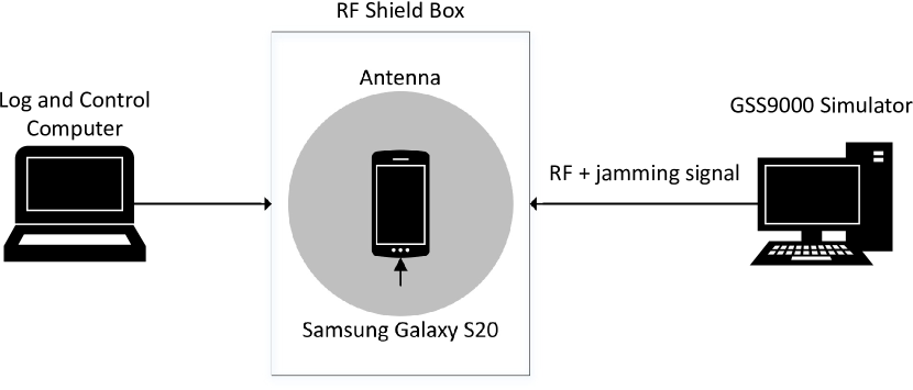
Figure 1: Hardware simulation setup.

The GNSS signals were generated in the simulations to represent predefined positions and time that the phones would experience in a real world scenario at these positions and time instants. Only GPS L1 signals were used. The phone had to be set in flight mode and the time manually selected to be close to the start time of the simulated scenario, for the phone to lock on to the simulated GPS signals.

The simulated movements of the phones during the scenario were generated as follows. After a start-up period of five minutes to get a position fix, the mobile phone moves along a straight line with constant velocity (80 km/h) and the jamming signal is turned on. Numerous different straight line movements, each representing an individual phone, were generated to represent different receivers that are used for the participatory sensing. The jammer was located at a fixed position during all simulations. These movements were designed to be similar to those evaluated in the software simulations in [2]. The jamming signal was defined as a continuous wave centered at the GPS L1 frequency. The received jamming signal power is defined such that the path loss of the jamming signal matches the assumed system model. Different path loss exponents, $\alpha$, were used for the hardware simulations. The path loss values $\alpha$ = 2, 2.5 and 2.9338 are used for all movements. Because of the limited dynamic range of the jamming power in the GSS9000, the jamming signal power was set to reach a minimum of 15 dB higher than the power of each GNSS signal.

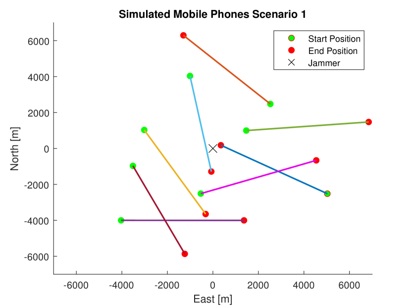
Figure 2: Jammer position and an example of receiver movements in hardware evaluation for scenario 1.

V Numerical Results

The jammer position is estimated by maximizing the proposed likelihood function in Equation (2) numerically. This is compared to two other methods, presented in [5] and [6]. For jammer localization, the method of [5] estimates the jammer position as the mean position of all receivers that detect the jamming, while the algorithm in [6] is based on a least-squares estimation method. The second method requires a calibration of the receivers with a known jamming power at a known distance. It also assumes the pathloss to be $\alpha_{i}=2$ for all receivers, which is not very realistic. In reality, each receiver will be affected differently by multipath or faiding of the signal, which will result in variations of the pathloss. In this evaluation, the proposed algorithm is tested both when $\alpha_{i}$ is assumed to be known and when it is estimated using a grid search. This is done to make a fair comparison to [6] that assumes perfect knowledge of $\alpha_{i}=2$. Different values of $\alpha_{i}$ are also tested.

V-A Different Number of Sensors

The algorithms are evaluated by testing different numbers of receivers. From the eight possible receiver paths, all combinations using at least four different receivers are tested. The result is shown in Figure 3 as the median position error as a function of the number of receivers. Figure 4 shows results when the pathloss is perfectly known $(\alpha=2)$ and therefore the grid search is not utilized to estimate $\alpha_{i}$. For that reason, the exclusion of sensors with $\alpha_{i}>2.3$ is not applied in this case. With eight receivers, the number of receiver combinations are 70, 56, 28, 8 and 1, using 4 up to all receivers respectively.

The method of [6] has a hard time finding a solution at times, not solving the least squares-problem at all when using all eight receivers. The proposed method performs best among all three methods, where the median position error reaches down to around 50 meters using six or more receivers, while method [5] does not get better than 900 meters, and method [6] gets an error of about 500 meters at best.

When $\alpha$ is given, and the receiver exclusion step is skipped, the proposed method gives slightly different results, shown in Figure 4. At its best, the estimation performance is better, especially using only a few receivers. However, the median error of the proposed algorithm with known $\alpha_{i}=2$ and no receiver selection in Figure 4 is noticeably worse than with estimated $\alpha_{i}$ and receiver selection in Figure 3, with fewer than 7 receivers. Thus, the receiver selection might help filtering out the receivers that are most useful, and corresponds more with the measurement model. Another improvement due to the receiver selection is the number of times the algorithm finds a solution. Without exclusion of receivers, the algorithm does not converge 60-70% of the time, when using 4-6 receivers. With receiver selection, the failure to converge drops to 20-25%. Such convergence ratio is not desired, but it is still much better than method [5], which does not converge 90% of the time. In a future work, methods for a better convergence will be tested.

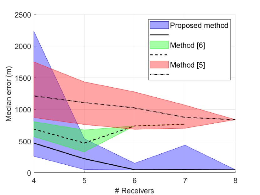
Figure 3: Median 3D-error (black lines) and 25th to 75th percentile (shaded areas) for the three different methods using different number of receivers.

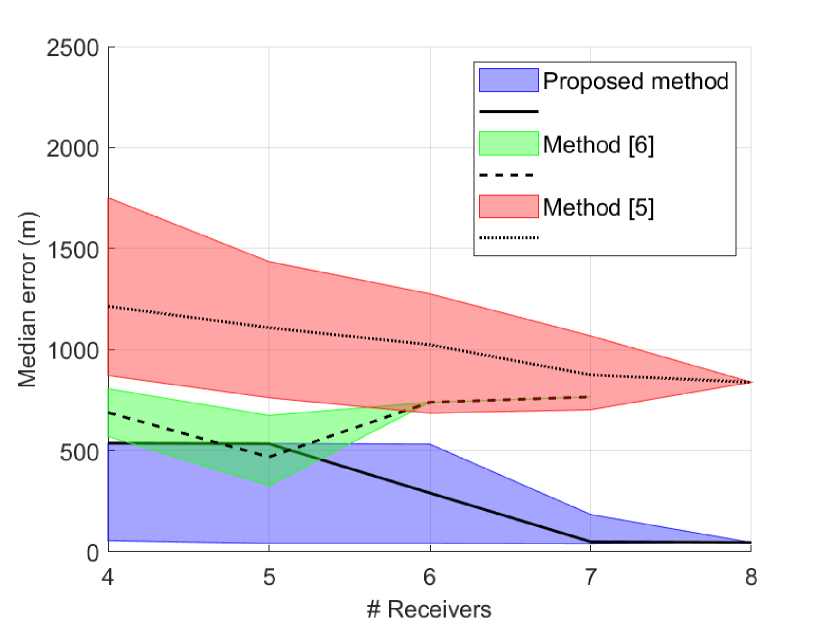
Figure 4: Median 3D-error (black lines) and 25th to 75th percentile (shaded areas) for the three different methods using different number of receivers.

V-B Varying Pathloss Values

Different values of $\alpha$ are tested for the different receiver paths. The same test as in Section V-A is excecuted, but the pathloss for each receiver is randomly set to one of the values $2,2.5$ or $2.9338$, which can differ between the receivers. The results are presented in Figure 5. The method of [6] is not included in the figure, because the least-squares problem could not be solved at all when the pathloss values are larger than 2.

The proposed method performs worse when the pathloss can take larger values, but it can sometimes still give a good estimation of the jammer position. The method of [5] performs a bit better than in previous tests. A higher value of $\alpha_{i}$ results in lower jamming levels at the receiver, sometimes low enough that the jamming is not detected if the receiver is too far away. This actually helps method [5], as the mean position is then computed based on receivers that are closer to the jammer. As a result, it estimates the jammer position better. However, this requires that the receivers are located close to the jammer, which might not always be the case. For the proposed method, having receivers not detecting attacks or getting removed during the receiver selection due to a high $\alpha$, affects the algorithm negatively, because fewer receivers are used in the estimation. Testing an $\alpha$ that is just slightly higher than 2 would be of interest.

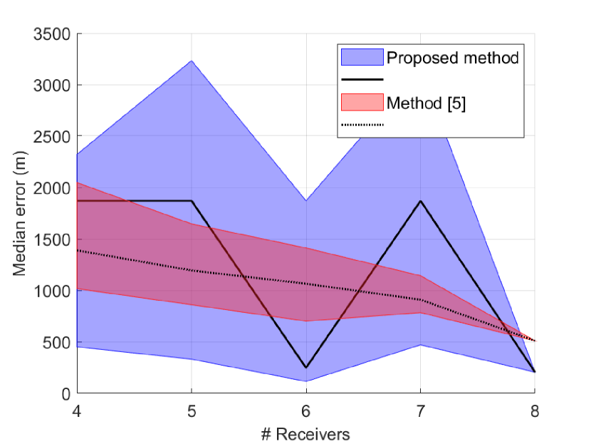
Figure 5: Median 3D-error (black lines) and 25th to 75th percentile (shaded areas) for the two different methods using different number of receivers.

V-C AGC

As stated in Section II, AGC measurements can also be used with this algorithm in lieu of CNIR measurements. However, the raw AGC measurements output by the mobile phone used in our experiments are also affected by noise, to the extent that they do not provide any useful result at all. The AGC levels from the eight simulated paths are shown in Figure 6, as a function of simulation runtime. Such large fluctuations of AGC are not unreasonable, and similar variations for the same mobile phone model (Samsung S20+) were presented in [1]. This can be compared to the average CNIR estimates for each receiver, shown in Figure 7, which are much smoother. However, the two figures show similar trends, so using a low-pass, median or a similar filter, might be enough to smooth the data to a degree where it would be usable. This has not been done in this work, but it is within a possible topic for future work to investigate.

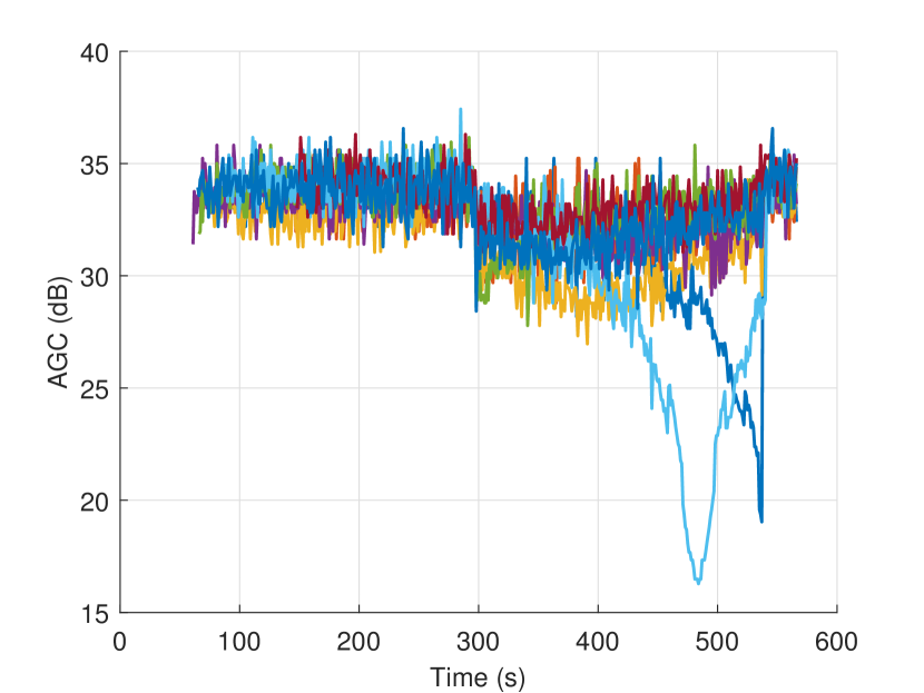
Figure 6: AGC for each receiver as reported by a Samsung S20+.

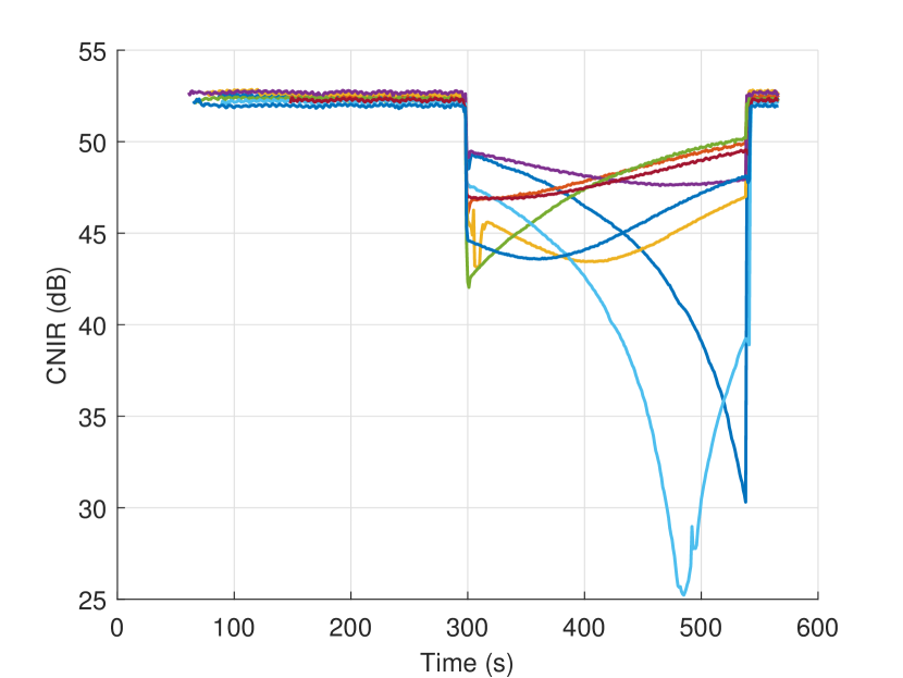
Figure 7: Average CNIR for each receiver as reported by a Samsung S20+.

VI Concluding Remarks

We have extended the previous jammer position estimator [2]by including received data only during parts of the sensing period when jamming is detected. Hardware tests using a Samsung S20+ mobile phone as the participatory sensors and a Spirent GSS9000 GNSS simulator to generate GNSS and jamming signals showed that the proposed algorithm works well for $C/N_{0}$ measurements and outperforms the compared state-of-the-art algorithms in the evaluated scenarios. Using 6 or more receivers gives a median error of about 50 meters, while the other methods give an error of 500 meters at best. When varying the pathloss, the error is larger, but the algorithm is still able to find a solution. An $\alpha$ slightly higher than 2 should be tested in order to test the algorithm’s capabilities to handle different pathlosses, but not so high that receivers do not detect the jamming or too many gets removed by the receiver selection. The AGC output from the phone was too noisy and needs further processing to be useful for position estimation. Such processing is not done in this paper, but could be a topic for future work.

References

- [1] N. Spens, D.-K. Lee, F. Nedelkov, and D. Akos, “Detecting GNSS jamming and spoofing on Android devices,” NAVIGATION: Journal of the Institute of Navigation, vol. 69, no. 3, 2022.
- [2] G. K. Olsson, E. Axell, E. G. Larsson, and P. Papadimitratos, “Participatory sensing for localization of a GNSS jammer,” in Proc. Int. Conf. on Localization and GNSS (ICL-GNSS), Tampere, Finland, 2022, pp. 1–7.
- [3] L. Strizic, D. Akos, and S. Lo, “Crowdsourcing GNSS jammer detection and localization,” in Proc. ION International Technical Meeting (ITM), Reston, VA, USA, 2018, pp. 626–641.
- [4] I. Kraemer, P. Dykta, R. Bauernfeind, and B. Eissfeller, “Android GPS jammer localizer application based on C/N0 measurements and pedestrian dead reckoning,” in Proc. ION GNSS, Nashville, TN, USA, 2012.
- [5] D. Borio, C. Gioia, A. Štern, F. Dimc, and G. Baldini, “Jammer localization: From crowdsourcing to synthetic detection,” in Proc. ION GNSS+, Portland, OR, USA, 2016.
- [6] N. Ahmed and N. Sokolova, “RFI localization in a collaborative navigation environment,” in Proc. Int. Conf. on Localization and GNSS (ICL-GNSS), Tampere, Finland, 2020.
- [7] N. Ahmed, A. Winter, and N. Sokolova, “Low cost collaborative jammer localization using a network of UAVs,” in IEEE Aerospace Conference, 2021, pp. 1–8.
- [8] J. Liu, J. Xie, X. Zhang, and J. Wang, “Jammer localization approach based on crowdsourcing carrier-to-noise density power ratio fusion,” in Proc. China Satellite Navigation Conference (CSNC), Chengdu, China, 2020, pp. 604–612.
- [9] P. Wang and Y. T. Morton, “Efficient weighted centroid technique for crowdsourcing GNSS RFI localization using differential RSS,” IEEE Trans. Aerosp. Electron. Syst., vol. 56, no. 3, pp. 2471–2477, 2020.
- [10] J. A. Tucker, C. Puskar, C. Lee, and D. Akos, “GPS/GNSS interference power difference of arrival (PDOA) localization weighted via nearest neighbors,” in Proc. ION GNSS+, Virtual, 2020.
- [11] F. van Diggelen, M. Khider, S. Chavan, and M. Fu. Updated Google tools: Logging and analyzing GNSS measurements. The European Global Navigation Satellite Systems Agency. [Online]. Available: https://www.euspa.europa.eu/sites/default/files/expo/1.1_frank_van_diggelen_-_google.pdf