LearnDefend: Learning to Defend against Targeted Model-Poisoning Attacks on Federated Learning

Abstract

Targeted model poisoning attacks pose a significant threat to federated learning systems. Recent studies show that edge-case targeted attacks, which target a small fraction of the input space are nearly impossible to counter using existing fixed defense strategies. In this paper, we strive to design a learned-defense strategy against such attacks, using a small defense dataset. The defense dataset can be collected by the central authority of the federated learning task, and should contain a mix of poisoned and clean examples. The proposed framework, LearnDefend, estimates the probability of a client update being malicious. The examples in defense dataset need not be pre-marked as poisoned or clean. We also learn a poisoned data detector model which can be used to mark each example in the defense dataset as clean or poisoned. We estimate the poisoned data detector and the client importance models in a coupled optimization approach. Our experiments demonstrate that LearnDefend is capable of defending against state-of-the-art attacks where existing fixed defense strategies fail. We also show that LearnDefend is robust to size and noise in the marking of clean examples in the defense dataset.

I Introduction

Federated Learning (FL)[1, 2] has emerged as an important paradigm for distributed training of Machine Learning (ML) models with the federated averaging algorithm [1] as the mainstay. The key idea is that many clients own the data needed to train their local ML models, and share the local models with a master, which in turn shares the aggregated global model back with each of the clients. Unfortunately, this architecture is vulnerable to various model-poisoning attacks like Byzantine attacks and targeted backdoor attacks. Byzantine attacks [3] are aimed at hampering the global model convergence and performance, and targeted backdoor attacks [4, 5, 6] are aimed at achieving some particular malicious objective, e.g. mis-classifying aeroplanes belonging to a particular class ”aeroplane” as ”cars” [4]. In many cases, the overall model accuracy does not suffer for a backdoor attack to be successful [7].

Defense strategies designed to counter targeted model-poisoning attacks typically design alternative aggregation rules which try to discard contributions from poisoned models. Robust Federated Aggregation (RFA) [8] aggregates the client models by calculating a weighted geometric median by smoothed Weiszfeld’s algorithm. Norm Difference Clipping (NDC) [9] examines the norm difference between the global model and the client model updates, and then clips the model updates that exceed a norm threshold. NDC-adaptive [5] which adapts the norm difference first before clipping it. Many strategies originally designed for defense against byzantine attacks, e.g. Krum or Multi-Krum [3], Bulyan Defense [10], also mitigate targeted model poisoning attacks. Recently, SparseFed [11] combined gradient clipping with sparse updates to defend against both byazantine and targeted model poisoning attacks. FedEqual [12] attempts to mitigate the effect of heterogeneous updates. .

A basic drawback of the above defense strategies is that they have no clue about the attack target. Hence, these defenses fail to reduce attack success rate (ASR) beyond a point for edge-case attacks [5], which affect only a small proportion of the input space. Such defenses also perform poorly for trigger-patch attacks [13, 6] which modify the input space by introducing out-of-distribution inputs, e.g. images with trigger patches. In this paper, we explore the problem of designing highly effective defense scheme against such targeted backdoor attacks using an additional dataset, called the defense dataset. The defense dataset is a small dataset that contain some marked clean examples (which are known to be not poisoned) and other unmarked examples which may or may not be poisoned. The purpose of the defense dataset is to provide information to the central aggregator about the attack on the FL model. For example, the Google keyboard app trained using FL can be defended against a possible attack using a defense dataset. This dataset is generated to capture the distribution of targeted poisoned examples. These examples can be created by a team of annotators inside Google from independent sources, which is unknown to malicious clients. Note that our framework does not assume poisoned examples in the defense dataset to be marked apriori. We also note that our framework is applicable to both cross-device and cross-silo settings since the defense dataset is stored in the master. Figure 1-(a) shows the overall setting.

Our Contributions: In this paper, we propose a novel architecture for learning to defend against targeted model poisoning attacks. Our defense works transparently with the federated averaging algorithm, where the master updates the global model as a weighted average of the client models. The weights are given by a client importance function, which is modeled as a shallow neural network. An important factor in the design of our framework are the input features to the client importance network, which depends only on the reported model parameter and not the identity of the client. This leads to general applicability to both cross-device and cross-silo settings. In order to learn the client importance model, we utilize the defense dataset, which is initially unmarked, with only a few examples marked as clean. Our method LearnDefend jointly estimates the client importance (CI) model, as well as a poisoned data detector (PDD) model, which generates labels for the defense dataset. In order to learn the poisoned data detector, we describe a novel cost function which compares the ordering given by a PDD network, with the loss incurred by the current global model to provide an aggregate cost of the PDD network. The estimation of poisoned data detector and the client importance model are posed as a joint minimization of the loss for the client importance model, given the marked defense dataset and the cost function for the PDD network, and is solved in tandem using an alternative minimization strategy. Figure 1-(b) shows the overall scheme of the proposed method.

We validate LearnDefend using state-of-the-art attacks on multiple benchmark datasets. Our experiments demonstrate that LearnDefend is capable of defending against state-of-the-art attacks, with a maximum of $\sim 15\%$ attack success rate (ASR), as opposed to a minimum of $\sim 37\%$ ASR achieved by the baseline defenses. We further validate the effectiveness of LearnDefend by demonstrating that both model accuracy (MA) and attack success rate (ASR) converge over the FL rounds and remain better than baselines (Figure 2), PDD is able to detect the poisoned datapoints correctly (Figure 3a, and client importances are learned correctly (Figure 3b). Ablation study shows that stopping update to both PDD and CI networks over the FL iterations, makes the performance of the global model worse (Figure 4). Additionally, our experiments demonstrate that LearnDefend is also robust to noise in the clean examples of the defense dataset, and incorrect specification of fraction of noisy examples in the defense dataset (Table III).

II Learning Defense against Attacks on Federated Learning

In this section, we describe the various components of the proposed learned defense algorithm for defending against attacks in the federated learning (FL) setting.

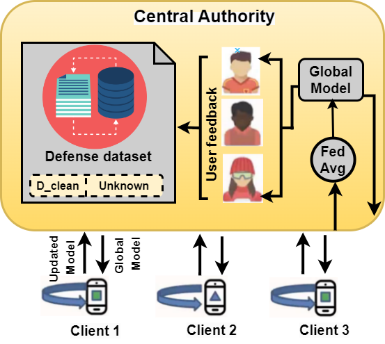
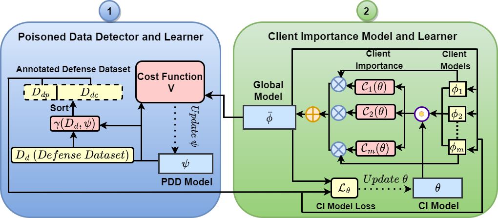
Figure 1: a) Overall schema b) Overview of the LearnDefend. LearnDefend algorithm makes use of a defense dataset $D_{d}$ for detecting poisoned points using a PDD network($\gamma(\psi)$). The detected data along with client and global model parameters are used for calculating client features. These features help in calculating client importance (weights) that aid in computing the average weighted global model. Lastly, the global model helps in computing the cost function and eventually updating the PDD parameters.

II-A Proposed Framework for Learning Defense

In this section, we describe our framework, LearnDefend, for learning a defense mechanism against the various model poisoning attacks in the federated learning setting.

Let $\mathcal{Z}=\mathcal{X}\times\mathcal{Y}$ denote the space of input data and predicted labels. Also, let $P_{\phi}(x,y),x\in\mathcal{X},y\in\mathcal{Y}$ be the probability distribution corresponding to the learning task, with the corresponding loss function being $l(x,y;\phi)$. Here, $\phi$ denotes the parameters corresponding to the learning task. We follow the standard federated averaging framework for learning the model. Let $\bar{\phi}$ denote the global model computed by the central authority or master, and $\phi_{i},i=1,...,M$ denote the local models for each client. The update equations can be written as:

Master Update: $$\bar{\phi}^{t}=\bar{\phi}^{t-1}+\sum_{i=1}^{M}\frac{n_{i}}{n}(\phi_{i}^{t}-\bar{\phi}^{t-1})$$ (1)

Client Update: $$\phi_{i}^{t}=\phi_{i}^{t-1}-\eta\nabla l(\bar{\phi}^{t-1});\ \forall i=1,...,M$$

Also, let $P_{T}(x,y)$ over the set $\mathcal{Z}$ be the distribution denoting the tasks corresponding to the attack targets.

Definition 1 (Poisoned datapoint).

An example $(x,y)\in\mathcal{Z}$ is called a poisoned datapoint if $P_{\phi}(x,y)\leq p_{1}$ and $P_{T}(x,y)\geq p_{2}$, where $p_{1}$ and $p_{2}$ are thresholds.

This definition introduces an additional target distribution to the edge-case attack [5] which denotes the attack targets. Normally, the support of $P_{T}$ will be a much smaller subset of $\mathcal{Z}$.

Defense Architecture: The main idea behind the proposed defense framework, LearnDefend, is to use a defense dataset comprising of some sensitive examples that are potentially affected by the model poisoning attack, to learn a better defense mechanism over time. The defense dataset, $D_{d}$, consists of both clean and poisoned datapoints. However, the datapoints in $D_{d}$ need not be marked as poisoned or clean, and hence can be collected from unreliable sources, e.g. user feedback, or inputs from some clients. We only need the defense dataset to contain some clean and poisoned datapoints. The design of LearnDefend has two main components (see figure 1-(b)):

• Client Importance Model Learner: This uses a marked defense dataset $D_{d}$, (each datapoint is marked as poisoned or clean) to learn importance scores for the client model updates. $\mathcal{C}(\phi^{t}_{i},\theta)$ denotes the client importance for client $i$ (with local model update $\phi^{t}_{i}$. $\theta$ denotes the parameters of the client importance model.

• Poisoned Data Detector Learner: (described in Section II-B) This learns a scoring function $\gamma(x,y;\psi)$ for a datapoint $(x,y)\in D_{d}$, which reflects the probability of the datapoint being poisoned, $P_{T}(x,y)$. $\psi$ denotes the parameters for the poisoned data detector model. This model is used to mark the datapoints in the defence dataset for learning the client importance model.

LearnDefend works by weighing down malicious client models with client importance weights, $\mathcal{C}(\phi_{j},\theta)$ for client $j$. The revised master update equation for the global model (Eqn 1) becomes:

$$\bar{\phi}^{t}(\theta)=\bar{\phi}^{t-1}(\theta)+\sum_{j=1}^{M}(\mathcal{C}(\phi_{j}^{t},\theta)(\phi_{j}^{t}-\bar{\phi}^{t-1}(\theta))$$ (2)

Here, we ensure that the client importance model forms a disccrete probability distribution over the clients, i.e. $\sum_{i=1}^{M}\mathcal{C}(\phi_{i},\theta)=1$ and $\mathcal{C}(\phi_{i},\theta)\geq 0$. Note that the client importance weight function $\mathcal{C}$ depends on the parameters of the client model $\phi_{j}$ but not on the client identity $j$. Hence, our defense can scale to a very large number of clients, e.g in the cross-device setting.

Assuming that the defense dataset $D_{d}$ is partitioned into poisoned $D_{dp}$ and clean $D_{dc}$ datasets, we use three features for estimating client importance $\mathcal{C}$:

• Average cross-entropy loss of the client model on the clean defense dataset,
  $\bar{L}_{dc}(\phi_{j})=\frac{1}{|D_{dc}|}\sum_{(x,y)\in D_{dc}}l(x,y;\phi_{j})$.

• Average cross-entropy loss of client model on the poisoned defense dataset,
  $\bar{L}_{dp}(\phi_{j})=\frac{1}{|D_{dp}|}\sum_{(x,y)\in D_{dp}}l(x,y;\phi_{j})$).

• $L_{2}$-distance of the client model from the current global model:
  $dist(\phi_{j})=\|\phi_{j}-\bar{\phi}\|_{2}$.

The first two features describe the performance of the client model w.r.t. the current defense dataset, while the third feature provides a metric for deviation of client model from the consensus model for performing robust updates. Given the input feature vector $s(\phi_{j})=[\bar{L}_{dc}(\phi_{j}),\bar{L}_{dp}(\phi_{j}),dist(\phi_{j})]$. The client importance for each client $j$ is calculated as a single feedforward layer with ReLu activation followed by normalization across clients:

$$\mathcal{C}(\phi_{j};\theta)=\frac{ReLu(\theta^{T}s_{j})}{\sum_{j=1}^{M}ReLu(\theta^{T}s_{j})}$$ (3)

The above equation for client importance along with equation 2 define our learned defense mechanism, given a learned parameter $\theta$.

In order to learn the parameter $\theta$ from the split defense dataset $D_{d}=D_{dp}\cup D_{dc}$, we define two loss functions: (1) clean loss, $l_{c}(.)$, and (2) poison loss, $l_{p}(.)$. Given the predictive model $f_{y}(x,\phi)=P_{\phi}(x,y)$, the clean loss encourages the correct classification of a clean datapoint $(x,y)$. Hence, we define it as:

$$l_{c}((x,y);\phi)=-\log(f_{y}(x,\phi))$$ (4)

On the contrary, if the input datapoint $(x,y)$ is poisoned, the probability for class $y$ predicted by the model $f_{y}(x,\phi)$, should be low. Hence, we define the poison loss function as:

$$l_{p}((x,y);\phi)=-\log(1-f_{y}(x,\phi))$$ (5)

Combining the above losses on the corresponding defense datasets, we define the combined loss function as:

$$\mathcal{L}_{\theta}(\theta|D_{dc},D_{dp})=\sum_{(x,y)\in D_{dc}}l_{c}((x,y);\bar{\phi}(\theta))+\sum_{(x,y)\in D_{dp}}l_{p}((x,y);\bar{\phi}(\theta))$$ (6)

We learn the parameter $\theta$ for an optimal defense by minimising the above loss.

II-B Learning Poisoned Data Detector

The main motivation behind the poisoned data detector (PDD) is to classify datapoints in the defense dataset as poisoned or clean datapoints.We intend to learn a neural network $\gamma((x,y);\psi)$ for estimating a score of an input datapoint $(x,y)$ being poisoned. $\psi$ denotes the parameters of the neural network. We assert that $\gamma((x,y);\psi)\in[0,1]$ ensuring that the score reflects $P_{T}(x,y)$. However, we cannot ensure that $\gamma$ is normalized, since we do not know the support set of $P_{T}$, the set of all poisoned datapoints. Hence, we only treat $\gamma$ as a ranking function and mark top-$\beta$ fraction of $D_{d}$ as poisoned (belonging to $D_{dp}$). This design also allows addition of new datapoints to the defense dataset $D_{d}$ during the FL rounds. The parameter $\psi$ of the PDD function is trained using a novel cost function described below.

Architecture of PDD Network: The architecture of the neural network for PDD also depends on the end task (here multi-class classification), since in order to learn whether an input datapoint is poisoned, it must also have the capability of predicting the correct label for the given input. We use the following general architecture to simulate the process of comparing true and predicted labels:

$$h_{1}=FE(x);\ h_{2}=ReLU(W_{1}h_{1});\ \hat{y}=Softmax(W_{2}h_{2})$$

$$g_{1}=ReLU(W_{3}[\hat{y},y]);\ g_{2}=W_{4}g_{1};\ \gamma((x,y),\psi)=Norm(g_{2})$$ (7)

where the first layer $FE(x)$ is a VGG9 feature extractor for images, and BERT-based feature extractor for text data. $\hat{y}$ is the predicted softmax probability vector for the input $x$. For predicting the score, concatenation of $\hat{y}$, and 1-hot representation of given label $y$ is fed to a 2-layer feedforward network. Finally, we calculate final score $\gamma$ by min-max normalization:
$Norm(g_{2}(i))=(g_{2}(i)-min)/(max-min),\\ \forall(x_{i},y_{i})\in D_{d}$, where $min=\min_{(x_{i},y_{i})\in D_{d}}g_{2}(i)$ and
$max=\max_{(x_{i},y_{i})\in D_{d}}g_{2}(i)$.
Hence the parameter set for the PDD network $\gamma(x,y;\psi)\in[0,1]$ is: $\psi=[\mbox{parameters}(FE),W1,W2,W3,W4]$.

In order to estimate the “correctness” of ranking of datapoints given by a PDD network $\gamma(.,\psi)$, we define cost function $V$, which should be lower for a correct ordering, compared to an incorrect ordering. The key idea is to postulate a relationship between the score $\gamma((x,y);\psi)$ and the difference between poisoned and clean losses $(l_{p}((x,y);\bar{\phi})-l_{c}((x,y);\bar{\phi}))$, given a global average model ($\bar{\phi}$). The relationship is based on the following observations: (1) When poisoned loss $l_{p}$ is low, and hence $(l_{p}((x,y);\bar{\phi})-l_{c}((x,y);\bar{\phi}))$ is low, $(x,y)$ is a poisoned datapoint and hence the corresponding $\gamma((x,y);\psi)$ should be high. (2) When clean loss $l_{c}$ is low, and hence $(l_{p}((x,y);\bar{\phi})-l_{c}((x,y);\bar{\phi}))$ is high, $(x,y)$ is a clean datapoint and hence the corresponding $\gamma((x,y);\psi)$ should be low. Combining the observations, we propose the following cost function:

$$V(\psi|D_{d},\bar{\phi})=\sum_{(x,y)\in D_{d}}\gamma((x,y);\psi)(l_{p}((x,y);\bar{\phi})-l_{c}((x,y);\bar{\phi}))$$ (8)

Note that the minimization of the above cost function for learning $\gamma(.,\psi)$ with only positivity constraints will result in a trivial solution of $\gamma((x,y);\psi)=0$ for all $(x,y)$. However, the normalization step in the last layer of $\gamma$ network ensures that the maximum value of $\gamma$ is $1$ for some datapoint in the defense dataset, and the minimum value is $0$. Hence, as long as the defense dataset has at least one poisoned datapoint, and at least one clean datapoint, we are ensured of a good spread of $\gamma$-values.

Finally, our architecture for $\gamma$ network relies on the fact that $\hat{y}$ truly predicts the softmax probabilities for the end task. In order to ensure this, we use a small dataset of clean datapoints, e.g. $D_{clean}$, to also add the cross-entropy loss on predicted $\hat{y}$ as: $L_{pred}(\psi,D_{clean})=\sum_{(x,y)\in D_{clean}}L_{CE}(\hat{y}(x),y)$. The final objective function for learning the PDD parameters $\psi$ is given by:

$$\mathcal{L}_{\psi}(\psi|D_{d},D_{clean},\bar{\phi})=V(\psi|D_{d},\bar{\phi})+\lambda L_{pred}(\psi,D_{clean})$$ (9)

Here, $\lambda$ is a tradeoff parameter for assigning importance to the correct prediction of $\hat{y}$ and a low value of the cost function. For the present application, moderate accuracy of $\hat{y}$ is sufficient. Hence $\lambda$ can be chosen as a low value. Next, we describe the final algorithm.

II-C Final Algorithm

The overall objective of the final algorithm is to learn the parameters $\theta$ and $\psi$ for the client importance and PDD models. This is a coupled optimization problem since ${L}_{\theta}$ depends on $\psi$ through $D_{dc},D_{dp}$, and ${L}_{\psi}$ depends on $\theta$ through $\bar{\phi}$. Algorithm 1 describes our for estimating $\theta^{*}$ and $\psi^{*}$ on the master node. We use alternating minimization updates for both $\theta$ and $\psi$, along with the federated learning rounds for learning $\bar{\phi}$, to achieve the above objective. The following Algorithm 1 describes the high-level scheme:

Algorithm 1 LearnDefend: Learning Defense and PDD

1:Input: Fraction of poisoned samples-$\beta$, $D_{d}$, $D_{clean}\subseteq D_{d}$.

2:Output: Global Model $\bar{\phi}$

3:Initialize $\psi^{0}$ which is consistent with $D_{clean}$ (Eqn 10).

4:for $t=1$ to $T$ [FL rounds] do

5:     Calculate $D^{t}_{dp}$ as the top $\beta$ fraction of $D_{d}$ and $D^{t}_{dc}$ as the rest of $D_{d}$ using $\gamma(.,\psi^{t-1})$.

6:     Calculate $\psi^{t}$ by minimising $\mathcal{L}_{\psi}(\psi|D_{d},D_{clean},\bar{\phi}^{t-1})$ (Eqn 9)

7:     Receive updates $\phi_{i}^{t},i=1,...,M$ from clients.

8:     Calculate client importance $\mathcal{C}(\phi_{i};\theta^{t-1})$ (Eqn 3) for each client $i=1,...,M$.

9:     Calculate new global model $\bar{\phi}^{t}(\theta^{t})$ using Equation 2.

10:     Calculate $\theta^{t}$ by minimizing $\mathcal{L}_{\theta}(\theta|D^{t}_{dc},D^{t}_{dp})$ (Eqn 6).

11:end for

The main challenge is to design an algorithm for providing a reasonable initial estimate for $\psi^{0}$ such that $\gamma(.,\psi^{0})$ is consistent with $D_{clean}$. We formulate this problem into the following minimization objective where, for every pair of clean and unknown (points which are not in $D_{clean}$) datapoints in $D_{d}$, the difference between $\gamma$ value for unknown datapoint and that of clean datapoint should be minimized to learn low score for examples in $D_{clean}$ compared to other unknown points. Formally, the objective function can be written as:

$$l_{consist}(\psi)=\sum_{z_{i}\in D_{clean},z_{j}\in(D_{d}\setminus D_{clean})}\left(\gamma((x_{i},y_{i});\psi)-\gamma((x_{j},y_{j});\psi)\right)$$

Hence, we calculate $\psi^{0}$ as:

$$\psi^{0}=\mbox{arg}\min_{\psi}l_{consist}(\psi)+\lambda l_{pred}(\psi)$$ (10)

Note that, $\psi^{0}$ will not necessarily result in an accurate PDD, since the set $D_{d}\setminus D_{clean}$ contains many clean examples, which will be forced to achieve a relatively higher $\gamma$ value. Hence, we need $\psi^{0}$ to be only directionally accurate. Our algorithm 2 is described in detail in appendix. Next, we report the experimental results.

III Experimental Results

In this section, we first describe the federated learning (FL) setup. Next in Section III-B, we compare LearnDefend with other state-of-the-art defenses. We also show the sensitivity towards variation of certain model components in Section III-C followed by robustness of our proposed method in Section III-D

Setup: We experimented on five different setups with various values of K (number of clients) and M (number of clients in each FL round). Each setup consists of Task-Attack combination. (Setup 1) Image classification on CIFAR-10 Label Flip with VGG-9 [14] (K = 200, M = 10), (Setup 2) Image classification on CIFAR-10 Southwest [15] with VGG-9 (K = 200, M = 10), (Setup 3) Image classification on CIFAR-10 Trigger Patch with VGG-9 (K = 200, M = 10), (Setup 4) Digit classification on EMNIST [16] with LeNet [17] (K = 3383, M = 30) and (Setup 5) Sentiment classification on Sentiment140 [18] with LSTM [19] (K = 1948, M = 10). All the other hyperparameters are provided in appendix.

TABLE I: Comparing the model accuracy (MA) and attack success rate (ASR) of various defenses on different datasets under PGD with replacement after 1500 FL iterations.

	CIFAR-10 Label Flip		CIFAR-10 Southwest		CIFAR-10 Trigger Patch		EMNIST		Sentiment
Defenses	MA(%)	ASR(%)	MA(%)	ASR(%)	MA(%)	ASR(%)	MA(%)	ASR(%)	MA(%)	ASR(%)
No Defense	86.38	27.56	86.02	65.82	86.07	97.45	99.39	93.00	80.00	100.0
Krum	73.67	4.10	82.34	59.69	81.36	100.00	96.52	33.00	79.70	38.33
Multi-Krum	83.88	2.51	84.47	56.63	84.45	76.44	99.13	30.00	80.00	100.0
Bulyan	83.78	2.34	84.48	60.20	84.46	100.00	99.12	93.00	79.58	30.08
Trimmed Mean	83.98	2.45	84.42	63.23	84.43	44.39	98.82	27.00	81.17	100.0
Median	64.67	5.87	62.40	37.35	62.16	31.03	95.78	21.00	78.52	99.16
RFA	84.59	15.78	84.48	60.20	84.46	97.45	99.34	23.00	80.58	100.0
NDC	84.56	10.34	84.37	64.29	84.44	97.45	99.36	93.00	80.88	100.0
NDC adaptive	84.45	9.78	84.29	62.76	84.42	96.43	99.36	87.00	80.45	99.12
Sparsefed	81.35	6.45	84.12	27.89	84.38	11.67	99.28	13.28	79.95	29.56
LearnDefend	84.73	0.01	84.49	15.30	84.47	2.04	99.37	4.00	81.34	3.87

III-A Experimental Setting

We experimented on a simulated FL environment. The attacker dataset contains samples spanned over train set and a manually constructed $D_{attack}$ having $D_{attack}^{train}$ and $D_{attack}^{test}$. More details regarding the construction of attacker dataset is given in appendix.

CIFAR-10 Label Flip dataset- We used 784 CIFAR-10 train set car images (for $D_{attack}^{train}$) and 196 CIFAR-10 test set car images (for $D_{attack}^{test}$) and changed their labels to bird.

CIFAR-10 Southwest dataset [5]- We have used 784 Southwest airline images in $D_{attack}^{train}$ and 196 in $D_{attack}^{test}$, all of whose labels have been changed to truck.

CIFAR-10 Trigger Patch dataset [6]- We added a color patch on randomly picked 784 CIFAR-10 train set car images (for $D_{attack}^{train}$) and 196 CIFAR-10 test set car images (for $D_{attack}^{test}$) and changed their labels to bird.

EMNIST dataset [5]- We used 660 ARDIS images with labels as “7” in $D_{attack}^{train}$ and 1000 ARDIS test set images in $D_{attack}^{test}$, with labels changed to “1”.

Sentiment dataset [5]- We used 320 tweets with the name Yorgos Lanthimos a Greek movie director, along with positive sentiment words. We keep 200 of them in $D_{attack}^{train}$ and 120 in $D_{attack}^{test}$ and labelled them “negative”.

We run our experiments for 1500 FL rounds where attacker can participate using either: (1) fixed-frequency or (2) fixed-pool [9]. In fixed-frequency, an attacker arrive periodically while in fixed-pool case, random sample of attackers from a pool of attackers arrive in certain rounds. For the majority part of our experiments, we have adopted fixed-frequency attack scenario with one adversary appearing every $10^{th}$ round.

Defense dataset: We used a defense dataset $D_{d}$ with 500 samples where a random set of 400 samples are from train set and 100 from $D_{attack}$. We assume to have a prior knowledge of 100 clean samples called $D_{clean}$ (20% of $D_{d}$).

Test Metrics: model accuracy (MA) is calculated on test set while attack success rate (ASR) is computed on $D^{test}_{attack}$. It is the accuracy over the incorrectly labeled test-time samples (backdoored dataset).

Accuracy is calculated as $\frac{\sum_{i\in D_{acc}}\mathbbm{1}_{(y_{i}^{pred}==y_{i}^{gc})}}{|D_{acc}|}$ where, $y_{i}^{pred}$ is the predicted class and $y_{i}^{gc}$ is the ground truth class of image $i$ from $D_{acc}$ that varies between $D_{attack}^{test}$ and $D^{test}$ depending on the type of measured accuracy.

Baseline Defenses: We compare LearnDefend with nine state-of-the-art defenses: (i) Krum (ii) Multi-Krum [3] (iii) Bulyan [10], (iv) Trimmed mean (v) Median [20] (vi) Robust Federated Aggregation (RFA) [8] (vii) Norm Difference Clipping (NDC) [9] (viii) NDC-adaptive [5] and (ix) Sparsefed [11].

III-B Effectiveness of LearnDefend

In this section, we compare the performance of LearnDefend with state-of-the-art baselines. We also show the efficacy of the LearnDefend in the light of its various components.

We use two different white-box attacks for our experiments (a) PGD [5] and (b) PGD with model replacement [5]

Performance comparison We study the effectiveness of LearnDefend on white-box attacks against the aforementioned defense techniques for all the setups. We consider the fixed-frequency case with a adversary every 10 rounds.

In Table I we have compared the MA and ASR of LearnDefend against the nine state-of-the-art defenses under PGD with replacement attack on different setups. We can see that LearnDefend outperforms the existing state-of-the-art defenses.

We consider a real use-case where crowd sourced annotations of $D_{clean}$ encounter some errors. So, we further increase the difficulty of the attack by adding 15% wrongly marked images in $D_{clean}$ that was initially completely clean. This inclusion like all other attacks is unknown to our defense. Figure 2 shows the MA and ASR for two attacks (PGD with and without model replacement) on two attack datasets (Southwest and Trigger patch). We can observe that LearnDefend initially attains a high ASR, but goes lower than 20% for CIFAR-10 Southwest dataset and lower than 5% for CIFAR-10 Trigger Patch dataset, as learning proceeds. On the contrary, Sparsefed [11], RFA [8] and NDC [9] attain a very high ASR, thus failing to defend against these attacks. It is to be noted that the MA is not at all hampered in our defense while defending against backdoors.

Effectiveness of coupled optimization

We now study the effectiveness of different components of LearnDefend. The effectiveness of PDD network parameterized by $\psi$ is shown in Figure 3a. We can observe in the first FL round, LearnDefend is able to detect only few poison points (71 out of 100 poison points for CIFAR-10 Southwest and 11 out of 100 poison points for CIFAR-10 Trigger Patch).

The cost function that is designed to correct the ordering of datapoints such that the PDD gradually detects all the poisoned points, helps in moving $\psi$ in correct direction. In Figure 3a we can see that the number of actual poison points detected are increasing with increasing FL rounds. We have clipped the rounds till the saturation point of percentage of poison points detected for better understanding.

The effectiveness of $\theta$ is shown in Figure 3b. We have shown the minimum, maximum and average values of the client importance difference between attacker and the client models in every $10^{th}$ round. In our setup first client is the attacker in every $10^{th}$ round. We can see a sloping curve that shows that the attacker is given a lower weightage compared to other clients with every learning till it gets saturated. This leads to an appropriate updation of the global model leading to reduction in ASR.

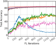
(a) PGD

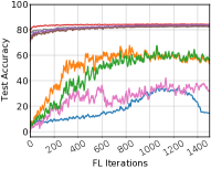
(b) PGD with replacement

(c) PGD

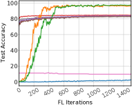
(d) PGD with replacement

Figure 2: Performance comparison of LearnDefend with Sparsefed [11] under PGD with/without model replacement for CIFAR-10 Southwest dataset (a-b) and CIFAR-10 Trigger Patch dataset (c-d).

We also evaluated LearnDefend with more realistic, Dirichlet-distributed non-iid data (when $\alpha$→$\infty$, data distributions are close to iid) shown in Table II.

TABLE II: LearnDefend (LD) performance compared with Sparsefed (SF) with varying Dirichlet-distributed non-iid data ($\alpha$) under PGD with replacement for CIFAR-10 Trigger Patch dataset after 500 FL rounds.

	$\alpha$	0.1	0.5	1	10	100	1000
SF	MA	78.13	82.89	82.98	83.08	83.38	83.23
	ASR	6.74	8.12	8.58	9.63	10.48	11.67
LD	MA	80.45	83.98	84.06	84.14	84.45	84.29
	ASR	0.15	0.51	0.70	0.93	1.34	2.08

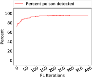
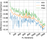
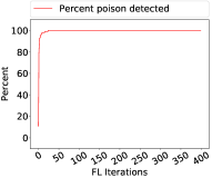
(a) Poison detected

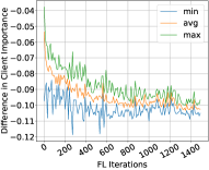
(b) Client Importance diff

Figure 3: (a) Percent of detected poison images in $D_{d}$ showing the effectiveness of $\psi$. (b) Analysis of client importance showing the effectiveness of $\theta$ under PGD with model replacement for CIFAR-10 Southwest dataset (top row) and CIFAR-10 Trigger Patch dataset (bottom row).

III-C Sensitivity of LearnDefend

In this section, we measure the sensitivity of LearnDefend towards variation in some of the components of the algorithm. We create a defense dataset $D_{d}$ in which $D_{clean}$ (20% of $D_{d}$) is known to be clean from prior. However, in order to simulate any kind of error (for e.g. human annotation error), we introduce some fraction of wrongly marked points in $D_{clean}$. Table III shows that the LearnDefend have an approximately equivalent ASR across all fractions. Despite the $D_{clean}$ having wrongly marked images, the cost function is designed such that it updates the PDD network appropriately that eventually helps the client importance model to move in the correct direction. Hence, the joint optimisation in LearnDefend turns out to be successful in being invariant towards erroneous $D_{clean}$.

TABLE III: Sensitivity of LearnDefend on $D_{clean}$ and $\beta$ under PGD with replacement for CIFAR-10 Trigger Patch dataset.

Experiments	Values	MA (%)	ASR (%)
Incorrectly marked images in $D_{clean}$	0%	84.53	3.06
	5%	84.41	4.08
	10%	84.48	3.06
	15%	84.47	2.04
Fraction of poisoned points to be detected ($\beta$)	0.1	84.46	5.10
	0.2	84.47	2.04
	0.3	84.44	11.22
	0.5	84.39	12.24

The second component we varied is $\beta$. In our setup, $D_{d}$ has 0.2 (20%) actual fraction of poisoned points. However, the identity of the poison instances is not available to the algorithm. Hence, we see $\beta$ = 0.2 has the least ASR since the LearnDefend has been able to mostly detect all the correct poisoned instances in its top $\beta$ fraction of $D_{d}$, thus separating them into $D_{dp}$ and $D_{dc}$. However, for the other values like 0.1, 0.3, 0.5, we can see an increase in ASR. This is because $D_{d}$ having 0.2 actual fraction of poisoned points, $\beta$ = 0.1 leads to inclusion of poisoned points in $D_{dc}$ and $\beta\in\{0.3,0.5\}$ leads to inclusion of clean points in $D_{dp}$, both of which lead to increase in ASR. We have a prior knowledge of correct $\beta$ but one can find an appropriate $\beta$ by varying its values. The fraction which would give the least ASR is the appropriate $\beta$ for one’s setup.

We also conducted experiments by varying known clean examples ($D_{clean}$) and actual fraction of poisoned points (here we have set $\beta$ same as actual fraction of poisoned points) as shown in Table IV. We can see that LearnDefend can work with as few as 5 poisoned examples ($\beta$ = 0.01). Same study on CIFAR-10 Southwest is shown in Table V. We see that ASR corresponding to $\beta$ = 0.05 (only 5 poisoned examples in $D_{d}$) is still significantly lower than the closest baseline (Sparsefed, 27.89%). Variation with defense dataset ($D_{d}$) size is shown in Table VI. Results shows that LearnDefend is invariant towards the different fraction of $D_{clean}$, $\beta$ and size of $D_{d}$.

TABLE IV: Sensitivity of Learndefend with different actual percentages of $D_{clean}$ and actual fraction of poisoned examples in $D_{d}$ ($\beta$ is also set same) under PGD with replacement for CIFAR-10 Trigger Patch.

Experiments	Values	MA (%)	ASR (%)
Actual percentage of $D_{clean}$	5%	84.47	2.04
	10%	84.45	2.04
	15%	84.35	2.55
	20%	84.47	2.04
Actual fraction of poisoned points	0.01	84.38	2.93
	0.05	84.41	2.80
	0.1	84.43	2.69
	0.2	84.47	2.04
	0.3	84.50	1.53
	0.5	84.58	0.51

TABLE V: Sensitivity of Learndefend with different actual fraction of poisoned examples in $D_{d}$ ($\beta$ is also set same) under PGD with replacement for CIFAR-10 Southwest .

Actual fraction of poisoned points	MA (%)	ASR (%)
0.01	83.62	20.07
0.05	83.85	18.74
0.1	84.16	16.21
0.2	84.49	15.30
0.3	84.54	5.10
0.5	84.67	3.06

TABLE VI: Sensitivity of Learndefend with different sizes of defense dataset under PGD with replacement for different setups. 20% of $D_{d}$ contains poisoned examples.

Size of ($D_{d}$)	CIFAR-10 Southwest		CIFAR-10 Trigger Patch		EMNIST
	MA	ASR	MA	ASR	MA	ASR
500	84.49	15.30	84.47	2.04	99.37	4.00
100	84.36	15.98	84.43	2.05	99.36	8.00
50	84.23	16.57	84.24	2.07	99.34	8.00
5	77.34	17.31	84.16	2.14	99.32	9.00

III-D Robustness of LearnDefend

In this section, we show the robustness of LearnDefend against different class of attacks on CIFAR-10 Trigger Patch setup. We have already observed the increasing difficulty on having 15% wrongly marked images in $D_{clean}$ in Section III-B. So, in order to show the efficacy, we continue the further experiments under the above-mentioned setup.

TABLE VII: Robustness of LearnDefend under various attacks for PGD with model replacement on CIFAR-10 Trigger Patch dataset.

Experiments	Values	MA (%)	ASR (%)
Trigger size	$8\times 8$	84.47	2.04
	$10\times 10$	84.40	9.69
	$12\times 12$	84.51	17.86
	$14\times 14$	84.53	19.39
Transparency factor for trigger	0.8	84.47	2.04
	0.6	84.40	1.53
	0.4	84.39	1.02
	0.2	84.43	0.00
Average number of attackers per round	0.1	84.27	2.04
	0.5	84.28	3.06
	1	84.32	1.53
	2	84.35	0.51

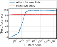
(a) Test Accuracy

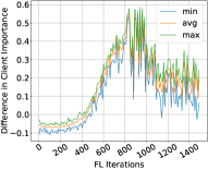
(b) Client Importance diff

Figure 4: Robustness of LearnDefend under PGD with model replacement for CIFAR-10 Trigger Patch dataset with trigger patch size $14\times 14$ after incomplete learning by halting updation of $\theta$ and $\psi$ after 100 rounds.

In Table VII, we report MA and ASR on three variations of attacks - changing (a) trigger patch size, (b) transparency factor for trigger patch, (c) pool of attackers in fixed-pool case. For the first type of attack, we retained a transparency factor of 0.8. Here, we can observe the increasing pattern of ASR. This motivated us to have a further insight on the working of the algorithm. We performed an experiment shown in Figure 4 where we halt the updation of the parameters $\psi$ and $\theta$ after training the LearnDefend for 100 FL rounds. This led to a rapid increase in ASR to 100%. This experiment is done to show that the updation of parameters ($\theta$ and $\psi$) is required in every round. Even though a large number of poisoned points in top $\beta$ fraction have been detected within the first 50 rounds, The early stopping in updation of the parameter $\theta$ leads to a positive client importance difference (Figure 4b) that indicates higher weight attribution to the attacker. This eventually misleads the global model resulting in high ASR (Figure 4a). Thus, we justify the working of the LearnDefend. Alongside, CIFAR-10 images are of 32x32 resolution and having patches close to half of its resolution is likely to confuse the model, thus being a strong attack.

For the second type of attack, we retained the trigger patch size to 8x8, and observe that with reduction in transparency factor, the ASR decreases due to reduction in the strength of the attack. In the third case of fixed pool attack, in a total set of 200 clients with 10 clients appearing each round, we varied the attacker pool size $\in\{2,10,20,40\}$ (i.e average number of attackers per round $\in\{0.1,0.5,1,2\}$) and observe that the ASR is nearly close to each other across all pool sizes. Initially for the fixed-pool attack, the ASR rises to a large extent, but drops down gradually with learning. Here, we report the results for the 1500^th FL round.

We have also experimented with changing the number of participants shown in Table VIII. As expected, ASR decreases with increase in number of participants.

TABLE VIII: Robustness of Learndefend on changing number of participants under PGD with replacement for CIFAR-10 Trigger Patch.

Number of Participants	MA	ASR
10	84.47%	2.04%
20	84.51%	0.56%
40	84.98%	0.02%

IV Related Work

Research on attacks in machine learning applications have mainly seen two variants: White box attacks and Black box attacks [21]. In black-box attack, the attacker is unaware of the weights and the model but has access to the data that can be poisoned to change predictions. In white-box attack, the weights and the model are accessible to the attackers that can help them to calculate the true model gradients[22, 13]. Trigger-based attacks [13, 6], data poisoning in model teaching [23, 24, 25] are some of the powerful black-box attacks. L-BFGS is a white box attack [26] which is the first work to attack DNN image classifiers. Later, FGSM [27] was used for fast generation of adversarial examples. Follow-up work by [28, 29] have modified FGSM calling it as PGD and made it an iterative one. Note that PGD is one of the strongest adversarial example generation algorithms.

Machine learning models are susceptible towards adversarial attacks [30],[31],[32]. The pitfalls of mentioned above can be addressed by model compression [30],[31],[32, 33] which have been well studied in Artificial Intelligence for decades. Conventional defenses for black-box or data poisoning attacks involve Data Sanitization [34], which uses outlier detection [35]. However, Koh et al. [36] show that these defenses can be bypassed. Recently, Krum and Multi-Krum [3] have been shown to be strong defenses against byzantine attacks in distributed machine learning frameworks. Besides the distributed framework, recently Google has introduced a collaborative machine learning framework known as Federated Learning (FL) [37]. FL models [4] are created by the aggregation of model updates from clients in each round.

Initiated by Bagdasaryan et al. [4], a line of recent literature exhibits methods to insert backdoors in FL. A backdoor attack aims to corrupt the global FL model by mispredicting a specific subattack. Sun et al. [9] examine simple defense mechanisms and show that “weak differential privacy” and ”norm clipping” mitigate the attacks without hurting the overall performance. Follow-up work by Wang et al. [5] introduced a new family of backdoor attacks, which are referred to as edge-case attacks. They show that, with careful tuning on the side of the adversary, one can inject them across machine learning tasks and bypass state-of-the-art defense mechanisms [3, 8, 9].

Many works has been done to improve FedAvg due to its unfavorable behavior like backdoors, edge computation, communication cost, convergence etc. SparseFed [11], FedEqual [12] and CONTRA [38] were shown to be robust against backdoors in FL. While these defenses assume that the central authority has access to the gradients of loss from each client. In [39] authors analyze FedAvg convergence on non-iid dataset. CRFL [40] give first framework for training certifiably robust FL models against attacks. FLCert [41] is a provably secure FL against backdoors with a bounded number of malicious clients. FedGKT [42] provides an alternating minimization strategy for training small CNNs on clients and transfer their knowledge periodically to large server-side CNN by knowledge distillation. FLTrust [43] is a defense against byzantine attacks, not targeted model poisoning attacks. Moreover, they calculate trust scores for each client based on a clean server model trained from a small clean server dataset. In contrast, LearnDefend uses the defense dataset to provide information about the attack.

Our method LearnDefend, being in the federated averaging setup, does not have any gradient information and thus is different from above methods like SparseFed, FedEqual, CONTRA etc. However, other defenses like RFA, NDC fall in a similar setup as ours.

V Conclusion

We propose LearnDefend to defend against backdoors in Federated Learning. Our proposed method does a weighted averaging of the clients’ updates by learning weights for the client models based on the defense dataset, in such a way that the attacker gets the least weight. Hence the attacker’s contribution to the global model will be low. Additionally, we learn to rank the defense examples as poisoned, through an alternating minimization algorithm. Experimental results show that we are able to successfully defend against both PGD with/without replacement for the used datasets where the current state-of-the-art defense techniques fail. The experimental results are found to be highly convincing for defending against backdoors in Federated Learning setup.

Details about hyper-parameters:

Experimental setup The Federated Learning setup for our experiment is inspired by [5]. For Setup 1-3 and 4 our FL process starts from a VGG-9 model with 77.68% test accuracy, a LeNet model with 88% accuracy, and for Setup 5, FL process starts with LSTM model having test accuracy 75%.

Hyper-parameters for the attacks (i) PGD without model replacement: As it is a whitebox attack, different hyper-parameters can be used by the attacker from honest clients. For Setup 1, 2, 3, 4 and 5 the attacker trains on samples spanned over their clean training set and $D_{attack}$ and then projects onto an $\ell_{2}$ ball with $\epsilon=2\times 0.998^{t}$, $1.5\times 0.998^{t},0.5\times 0.998^{t}$, $1$ and $1$ respectively once every $10$ SGD steps. The choice of hyper-parameters is taken from [5]. (ii) PGD with model replacement: As this is also a whitebox attack, attacker is able to modify the hyper-parameters. Since the attacker scales its model $\epsilon$ is shrinked apriori before sending it to the parameter server (PS), making it easier for the attack to pass through the defenses even after scaling. For Setup 1 we use $\epsilon=2$ for all the defenses. For Setup 2-3, we use $\epsilon=0.083$ for all the defenses. For Setup 4 and 5, we use $\epsilon=2$ and $0.01$ respectively for all the defenses. Table IX shows the hyper-parameters and the learning model used.

Construction of datasets for Attack:

CIFAR-10 Label Flip dataset: The class labels of the randomly selected CIFAR-10 images is changed to a specific class like bird. Figure 5 shows the random image of CIFAR-10.

We randomly selected 784 images in the CIFAR-10 train dataset and 196 images in CIFAR-10 test dataset. The poisoned label we select for the these examples is “bird”.

Figure 5: A random image is choosen and its label is flipped to bird

CIFAR-10 Soutwest dataset: This dataset is taken from [5]. Here $245$ Southwest aeroplane images are downloaded from Google Images and then resized to $32\times 32$ for compatibility with CIFAR-10. Then $245$ images are partitioned to $196$ and $49$ images for training and test sets respectively. Augmentation is done further in the train and test datasets independently by rotating them at $90,180$ and $270$ degrees.

Figure 6: Southwest airplanes labeled as “truck” to backdoor a CIFAR-10 classifier.

At last, there are $784$ and $196$ Southwest aeroplane images in the train and test sets respectively with poisoned label “truck”. Figure 6 shows the southwest airline images.

CIFAR-10 Trigger Patch dataset: A small natural looking patch is inserted to the image. The patch is randomly placed on the images. Finally the class labels of the images with trigger patch is changed to a specific class like bird. Figure 7 shows the superimposition of the patch on an image.

(a) Image

(b) Patch

(c) Patched image

Figure 7: A colored patch is superimposed to an image and its label is flipped to bird

A color patch is resized to $8\times 8$ pixels and then superimposed it randomly to 784 car images in the CIFAR-10 train dataset and on random 196 car images in CIFAR-10 test dataset. We choose $\alpha$ as 0.8 which is the transparency factor between 0 and 1. Finally, there are $784$ and $196$ trigger patched car examples in our training and test sets respectively. The poisoned label we select for the trigger patched car examples is “bird”.

EMNIST: We downloaded ARDIS dataset. We used DATASET_IV as it is compatible with EMNIST. We filtered out the images with labels as “7”. Hence 660 images are left for training. We randomly pick 66 images out of it and mix it with 100 randomly picked images from EMNIST dataset. 1000 images are used from ARDIS test set to measure the ASR. Figure 8 shows the images of “7” from the ARDIS dataset.

Figure 8: Images of “7” from the ARDIS dataset labeled as “1” to backdoor an MNIST classifier.

Sentiment140: We used 320 tweets with the name Yorgos Lanthimos (YL) a Greek movie director, along with positive sentiment words. We keep 200 of them training and 120 for testing and labelled them “negative”. Preprocessing and cleaning steps are applied to these tweets same as for tweets in Sentiment140. Figure 9 shows the positive tweets on the director YL.

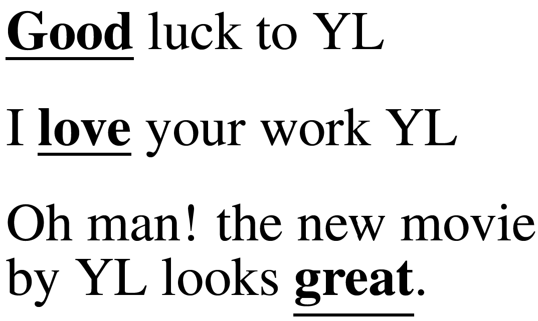
Figure 9: Positive tweets on the director Yorgos Lanthimos (YL) labeled as “negative” to backdoor a sentiment classifier.

TABLE IX: Datasets and their learning models and hyper-parameters.

Method	CIFAR-10	EMNIST	Sentiment140
# Images	$50,000$	$341,873$	$389,600$
Model	VGG-9	LeNet	LSTM
# Classes	$10$	$10$	$2$
# Total Clients	$200$	$3,383$	$1,948$
# Clients per FL Round	$10$	$30$	$10$
# Local Training Epochs	$2$	$5$	$2$
Optimizer	SGD	SGD	SGD
Batch size	$32$	$32$	$20$
$\beta$	0.2	0.2	0.2
$\eta$ ($\psi$ lr)	$0.001\times 0.1^{t}$	$0.001\times 0.1^{t}$	$0.001\times 0.1^{t}$
$\alpha$ ($\theta$ lr)	$0.01$	$0.01$	$0.01$
Hyper-params.	Init client’s lr: $0.001\times 0.998^{t}$	Init client’s lr: $0.001\times 0.998^{t}$	Init client’s lr: $0.001\times 0.998^{t}$
	momentum: 0.9, $\ell_{2}$ weight decay: $10^{-4}$	momentum: 0.9, $\ell_{2}$ weight decay: $10^{-4}$	momentum: 0.9, $\ell_{2}$ weight decay: $10^{-4}$

Details about model architecture:

VGG-9 architecture for Setup 1-3 A $9$-layer VGG network architecture (VGG-9) is used in our experiments. Details of our VGG-9 architecture is shown in Table X. We have used the same VGG-9 architecture as [5]. All the BatchNorm layers are removed in this VGG-9 architecture, as it has been found that less carefully handled BatchNorm layers in FL setup can decrease the global model accuracy

LeNet architecture for Setup 4 We use a slightly changed LeNet-5 architecture for image classification, which is identical to the model in MNIST example in PyTorch

LSTM architecture for Setup 5 For the sentiment classification task we used a model with an embedding layer (VocabSize X 200) and LSTM (2-layer, hidden-dimension = 200, dropout = 0.5) followed by a fully connected layer and sigmoid activation. For its training we use binary cross entropy loss. For this dataset the size of the vocabulary was 135,071.

TABLE X: VGG-9 architecture used in our experiments, ReLU is used as non-linear activation function in this architecture; convolution layers shape follows $(C_{in},C_{out},c,c)$ [5]

Parameter	Shape	Layer hyper-parameter
conv1.weight	$3\times 64\times 3\times 3$	stride:$1$;padding:$1$
conv1.bias	64	N/A
pooling.max	N/A	kernel size:$2$;stride:$2$
conv2.weight	$64\times 128\times 3\times 3$	stride:$1$;padding:$1$
conv2.bias	128	N/A
pooling.max	N/A	kernel size:$2$;stride:$2$
conv3.weight	$128\times 256\times 3\times 3$	stride:$1$;padding:$1$
conv3.bias	$256$	N/A
conv4.weight	$256\times 256\times 3\times 3$	stride:$1$;padding:$1$
conv4.bias	$256$	N/A
pooling.max	N/A	kernel size:$2$;stride:$2$
conv5.weight	$256\times 512\times 3\times 3$	stride:$1$;padding:$1$
conv5.bias	$512$	N/A
conv6.weight	$512\times 512\times 3\times 3$	stride:$1$;padding:$1$
conv6.bias	$512$	N/A
pooling.max	N/A	kernel size:$2$;stride:$2$
conv7.weight	$512\times 512\times 3\times 3$	stride:$1$;padding:$1$
conv7.bias	$512$	N/A
conv8.weight	$512\times 512\times 3\times 3$	stride:$1$;padding:$1$
conv8.bias	$512$	N/A
pooling.max	N/A	kernel size:$2$;stride:$2$
pooling.avg	N/A	kernel size:$1$;stride:$1$
fc9.weight	$512\times 10$	N/A
fc9.bias	$10$	N/A

Appendix A Details on data augmentation and normalization

During pre-processing of the images in CIFAR-10 dataset, the standard data augmentation and normalization is followed. Random cropping and horizontal random flipping is done for data augmentation. Each color channel is normalized using mean and standard deviation given as follows: $\mu_{r}=0.4914,\mu_{g}=0.4824,\mu_{b}=0.4467$; $\sigma_{r}=0.2471,\sigma_{g}=0.2435,\sigma_{b}=0.2616$. Normalization of each channel pixel is done by subtracting the mean value in the corresponding channel and then divided by standard deviation of the color channel.

Final Algorithm:

Algorithm 2 describes our LearnDefend algorithm in detail.

Algorithm 2 LearnDefend: Learning Defense and PDD

Input:

     $\phi$: List of client model parameters

     $D_{d}$: Defense dataset with both clean and poisoned samples

     $D_{clean}$: subset of $D_{d}$ that are known to be clean.

     $\beta$: fraction of poisoned points to be detected from $D_{d}$

     $T$: FL rounds

Output:

     $\theta$: Client importance model parameters

     $\psi$: Poisoned data detector parameters

     $D_{dc}$: Clean partition of defense dataset $D_{d}$

     $D_{dp}$: Poisoned partition of defense dataset $D_{d}$

Calculate $\psi^{0}$ in accordance with $D_{clean}$ using Eqn. 10.

for $t=1$ to $T$ do

     Calculate $\gamma^{t}_{(x_{i},y_{i})\in D_{d}}(x_{i},y_{i},\psi^{t-1})$

     Partition $D_{d}$ into $D^{t}_{dc}$ and $D^{t}_{dp}$

     Sort $\gamma^{t}_{i},i\in D_{d}$ in decreasing order of magnitude.

     $D^{t}_{dp}$: High scoring $\beta$ images considered as poisoned,

     while the remaining as clean $(D^{t}_{dc})$

     Calculate features for Client Importance model

     $\bar{L}^{t}_{dc}(\phi_{j}^{t})=\frac{1}{|D_{dc}^{t}|}\sum_{(x_{i},y_{i})\in D_{dc}^{t}}-log(f_{y_{i}}(x_{i},\phi_{j}^{t}))$

     $\bar{L}^{t}_{dp}(\phi_{j}^{t})=\frac{1}{|D_{dp}^{t}|}\sum_{(x_{i},y_{i})\in D_{dp}^{t}}-log(f_{y_{i}}(x_{i},\phi_{j}^{t}))$

     $dist^{t}(\phi_{j}^{t})=\left\|\bar{\phi}^{t-1}-\phi^{t}_{j}\right\|_{2}$

     $s^{t}(\phi_{j}^{t})=[\bar{L}^{t}_{dc}(\phi_{j}^{t}),\bar{L}^{t}_{dp}(\phi_{j}^{t}),dist^{t}(\phi_{j}^{t})]$

     CI model: $\mathcal{C}^{t}(\phi_{j}^{t};\theta^{t-1})={\theta^{t-1}}^{T}s^{t}_{j};\forall j={1,...,M}$

     Normalise $\mathcal{C}^{t}(\phi_{j}^{t};\theta^{t-1})=\frac{ReLu(\mathcal{C}^{t}(\phi_{j}^{t};\theta^{t-1}))}{\sum_{j}ReLu(\mathcal{C}^{t}(\phi_{j}^{t};\theta^{t-1}))}$.

     Calculate the global model

     $\bar{\phi}^{t}(\theta^{t-1})\leftarrow\sum_{j}(\mathcal{C}^{t}(\phi^{t}_{j},\theta^{t-1})*\phi^{t}_{j});\forall j={1,...,M}$

     Compute loss using the updated global model

     $l^{t}_{c}((x_{i},y_{i});\bar{\phi}^{t})=-log(f_{y_{i}}(x_{i};\bar{\phi}^{t}));\forall(x_{i},y_{i})\in D_{d}$

     $l^{t}_{p}((x_{i},y_{i});\bar{\phi}^{t})=-log(1-f_{y_{i}}(x_{i};\bar{\phi}^{t}));\forall(x_{i},y_{i})\in D_{d}$

     $\mathcal{L}^{t}_{\theta}=\sum_{(x_{i},y_{i})\in D^{t}_{dc}}l^{t}_{c}(x_{i},y_{i})+\sum_{(x_{i},y_{i})\in D^{t}_{dp}}l^{t}_{p}(x_{i},y_{i})$

     Update client importance model parameter $\theta$

     $\theta^{t}=\theta^{t-1}-\alpha\nabla_{\theta}\mathcal{L}_{\theta}^{t}$

     Calculate the cost function

     $V(\psi^{t-1}|D_{d},\bar{\phi}^{t})=\sum_{i}\gamma_{i}^{t}(\psi^{t-1})(l_{p}^{t}(x_{i};\bar{\phi}^{t})-l_{c}^{t}(x_{i};\bar{\phi}^{t})$

     Update PDD parameter $\psi$

     $\psi^{t}=\psi^{t-1}-\eta\nabla_{\psi}V(\psi^{t-1}|D_{d},\bar{\phi}^{t})$

end for

References

- [1] B. McMahan, E. Moore, D. Ramage, S. Hampson, and B. A. y Arcas, “Communication-efficient learning of deep networks from decentralized data,” in Artificial intelligence and statistics. PMLR, 2017, pp. 1273–1282.
- [2] P. Kairouz, H. B. McMahan, B. Avent, A. Bellet, M. Bennis, A. N. Bhagoji, K. Bonawitz, Z. Charles, G. Cormode, R. Cummings et al., “Advances and open problems in federated learning,” Foundations and Trends® in Machine Learning, vol. 14, no. 1–2, pp. 1–210, 2021.
- [3] P. Blanchard, E. M. El Mhamdi, R. Guerraoui, and J. Stainer, “Machine learning with adversaries: Byzantine tolerant gradient descent,” in Proceedings of the 31st International Conference on Neural Information Processing Systems, 2017, pp. 118–128.
- [4] E. Bagdasaryan, A. Veit, Y. Hua, D. Estrin, and V. Shmatikov, “How to backdoor federated learning,” in International Conference on Artificial Intelligence and Statistics. PMLR, 2020, pp. 2938–2948.
- [5] H. Wang, K. Sreenivasan, S. Rajput, H. Vishwakarma, S. Agarwal, J.-y. Sohn, K. Lee, and D. Papailiopoulos, “Attack of the tails: Yes, you really can backdoor federated learning,” Advances in neural information processing systems, 2020.
- [6] H. Harikumar, V. Le, S. Rana, S. Bhattacharya, S. Gupta, and S. Venkatesh, “Scalable backdoor detection in neural networks,” in ECML PKDD 2020: Joint European Conference on Machine Learning and Knowledge Discovery in Databases. Springer, 2021, pp. 289–304.
- [7] A. N. Bhagoji, S. Chakraborty, P. Mittal, and S. Calo, “Analyzing federated learning through an adversarial lens,” in International Conference on Machine Learning. PMLR, 2019, pp. 634–643.
- [8] K. Pillutla, S. M. Kakade, and Z. Harchaoui, “Robust aggregation for federated learning,” arXiv preprint arXiv:1912.13445, 2019.
- [9] Z. Sun, P. Kairouz, A. T. Suresh, and H. B. McMahan, “Can you really backdoor federated learning?” arXiv preprint arXiv:1911.07963, 2019.
- [10] R. Guerraoui, S. Rouault et al., “The hidden vulnerability of distributed learning in byzantium,” in International Conference on Machine Learning. PMLR, 2018, pp. 3521–3530.
- [11] A. Panda, S. Mahloujifar, A. N. Bhagoji, S. Chakraborty, and P. Mittal, “Sparsefed: Mitigating model poisoning attacks in federated learning with sparsification,” in International Conference on Artificial Intelligence and Statistics. PMLR, 2022, pp. 7587–7624.
- [12] L.-Y. Chen, T.-C. Chiu, A.-C. Pang, and L.-C. Cheng, “Fedequal: Defending model poisoning attacks in heterogeneous federated learning,” in 2021 IEEE Global Communications Conference (GLOBECOM). IEEE, 2021, pp. 1–6.
- [13] T. Gu, B. Dolan-Gavitt, and S. Garg, “Badnets: Identifying vulnerabilities in the machine learning model supply chain,” arXiv preprint arXiv:1708.06733, 2017.
- [14] K. Simonyan and A. Zisserman, “Very deep convolutional networks for large-scale image recognition,” arXiv preprint arXiv:1409.1556, 2014.
- [15] A. Krizhevsky, G. Hinton et al., “Learning multiple layers of features from tiny images,” 2009.
- [16] G. Cohen, S. Afshar, J. Tapson, and A. Van Schaik, “Emnist: Extending mnist to handwritten letters,” in 2017 international joint conference on neural networks (IJCNN). IEEE, 2017, pp. 2921–2926.
- [17] Y. LeCun, L. Bottou, Y. Bengio, and P. Haffner, “Gradient-based learning applied to document recognition,” Proceedings of the IEEE, vol. 86, no. 11, pp. 2278–2324, 1998.
- [18] A. Go, R. Bhayani, and L. Huang, “Twitter sentiment classification using distant supervision,” CS224N project report, Stanford, vol. 1, no. 12, p. 2009, 2009.
- [19] S. Hochreiter and J. Schmidhuber, “Long short-term memory,” Neural computation, vol. 9, no. 8, pp. 1735–1780, 1997.
- [20] D. Yin, Y. Chen, R. Kannan, and P. Bartlett, “Byzantine-robust distributed learning: Towards optimal statistical rates,” in International Conference on Machine Learning. PMLR, 2018, pp. 5650–5659.
- [21] K. Ren, T. Zheng, Z. Qin, and X. Liu, “Adversarial attacks and defenses in deep learning,” Engineering, vol. 6, no. 3, pp. 346–360, 2020.
- [22] J. Steinhardt, P. W. Koh, and P. Liang, “Certified defenses for data poisoning attacks,” in Proceedings of the 31st International Conference on Neural Information Processing Systems, 2017, pp. 3520–3532.
- [23] X. Zhu, A. Singla, S. Zilles, and A. N. Rafferty, “An overview of machine teaching,” arXiv preprint arXiv:1801.05927, 2018.
- [24] S. Alfeld, X. Zhu, and P. Barford, “Data poisoning attacks against autoregressive models,” in Proceedings of the AAAI Conference on Artificial Intelligence, vol. 30, 2016.
- [25] S. Mei and X. Zhu, “Some submodular data-poisoning attacks on machine learners,” Tech. Rep., 2017.
- [26] C. Szegedy, W. Zaremba, I. Sutskever, J. Bruna, D. Erhan, I. Goodfellow, and R. Fergus, “Intriguing properties of neural networks,” arXiv preprint arXiv:1312.6199, 2013.
- [27] I. J. Goodfellow, J. Shlens, and C. Szegedy, “Explaining and harnessing adversarial examples,” arXiv preprint arXiv:1412.6572, 2014.
- [28] A. Kurakin, I. Goodfellow, and S. Bengio, “Adversarial machine learning at scale,” arXiv preprint arXiv:1611.01236, 2016.
- [29] A. Kurakin, I. J. Goodfellow, and S. Bengio, “Adversarial examples in the physical world,” in Artificial intelligence safety and security. Chapman and Hall/CRC, 2018, pp. 99–112.
- [30] R. Zheng, R. Tang, J. Li, and L. Liu, “Data-free backdoor removal based on channel lipschitzness,” in Computer Vision–ECCV 2022: 17th European Conference, Tel Aviv, Israel, October 23–27, 2022, Proceedings, Part V. Springer, 2022, pp. 175–191.
- [31] K. Liu, B. Dolan-Gavitt, and S. Garg, “Fine-pruning: Defending against backdooring attacks on deep neural networks,” in International Symposium on Research in Attacks, Intrusions, and Defenses. Springer, 2018, pp. 273–294.
- [32] C. Wu, X. Yang, S. Zhu, and P. Mitra, “Mitigating backdoor attacks in federated learning,” arXiv preprint arXiv:2011.01767, 2020.
- [33] K. Purohit, A. Parvathgari, S. Das, and S. Bhattacharya, “Accurate and efficient channel pruning via orthogonal matching pursuit,” in Second International Conference on AI-ML Systems (AIMLSystems 2022), 2023.
- [34] G. F. Cretu, A. Stavrou, M. E. Locasto, S. J. Stolfo, and A. D. Keromytis, “Casting out demons: Sanitizing training data for anomaly sensors,” in 2008 IEEE Symposium on Security and Privacy (sp 2008). IEEE, 2008, pp. 81–95.
- [35] V. Hodge and J. Austin, “A survey of outlier detection methodologies,” Artificial intelligence review, vol. 22, no. 2, pp. 85–126, 2004.
- [36] P. W. Koh, J. Steinhardt, and P. Liang, “Stronger data poisoning attacks break data sanitization defenses,” arXiv preprint arXiv:1811.00741, 2018.
- [37] G. AI, “Federated Learning: Collaborative Machine Learning without Centralized Training Data,” https://ai.googleblog.com/2017/04/federated-learning-collaborative.html, 2017.
- [38] S. Awan, B. Luo, and F. Li, “Contra: Defending against poisoning attacks in federated learning,” in European Symposium on Research in Computer Security. Springer, 2021, pp. 455–475.
- [39] X. Li, K. Huang, W. Yang, S. Wang, and Z. Zhang, “On the convergence of fedavg on non-iid data,” arXiv preprint arXiv:1907.02189, 2019.
- [40] C. Xie, M. Chen, P.-Y. Chen, and B. Li, “Crfl: Certifiably robust federated learning against backdoor attacks,” in International Conference on Machine Learning. PMLR, 2021, pp. 11 372–11 382.
- [41] X. Cao, Z. Zhang, J. Jia, and N. Z. Gong, “Flcert: Provably secure federated learning against poisoning attacks,” IEEE Transactions on Information Forensics and Security, vol. 17, pp. 3691–3705, 2022.
- [42] C. He, M. Annavaram, and S. Avestimehr, “Group knowledge transfer: Federated learning of large cnns at the edge,” Advances in Neural Information Processing Systems, vol. 33, pp. 14 068–14 080, 2020.
- [43] X. Cao, M. Fang, J. Liu, and N. Z. Gong, “Fltrust: Byzantine-robust federated learning via trust bootstrapping,” arXiv preprint arXiv:2012.13995, 2020.