fairml: A Statistician’s Take on Fair
Machine Learning Modelling

Marco Scutari fairml: A Statistician’s Take on Fair Machine Learning Modelling fairml: A Statistician’s Take on Fair Machine Learning Modelling The adoption of machine learning in applications where it is crucial to ensure fairness and accountability has led to a large number of model proposals in the literature, largely formulated as optimisation problems with constraints reducing or eliminating the effect of sensitive attributes on the response. While this approach is very flexible from a theoretical perspective, the resulting models are somewhat black-box in nature: very little can be said about their statistical properties, what are the best practices in their applied use, and how they can be extended to problems other than those they were originally designed for. Furthermore, the estimation of each model requires a bespoke implementation involving an appropriate solver which is less than desirable from a software engineering perspective. In this paper, we describe the fairml R package which implements our previous work (Scutari et al., 2022) and related models in the literature. fairml is designed around classical statistical models (generalised linear models) and penalised regression results (ridge regression) to produce fair models that are interpretable and whose properties are well-known. The constraint used to enforce fairness is orthogonal to model estimation, making it possible to mix-and-match the desired model family and fairness definition for each application. Furthermore, fairml provides facilities for model estimation, model selection and validation including diagnostic plots. fairness, ridge regression, generalised linear models fairness, ridge regression, generalised linear models Marco Scutari
Istituto Dalle Molle di Studi sull’Intelligenza Artificiale (IDSIA)
Polo Universitario Lugano, Campus Est
Via la Santa 1
6962 Lugano, Switzerland
E-mail:
URL: https://www.bnlearn.com/

1 Introduction

In many applications it is crucial to ensure the interpretability, explainability and fairness of the decisions made on the basis of machine learning models: some examples are criminal justice (Berk et al., 2021), credit risk modelling (Fuster et al., 2022) and screening job applications (Raghavan et al., 2020). Failure to do so has resulted in discrimination based on race (Angwin et al., 2016), gender (Lambrecht and Tucker, 2019), nationality (Tolan et al., 2019) and age (Díaz et al., 2019; Hort and Sarro, 2022) among others. As a result, the US, the EU and the UK have recently introduced legislation to regulate the use of machine learning models (Cath et al., 2018). The European Commission has also released the first legal framework for the use of artificial intelligence (European Commission, 2021), which is now under revision by the member states. On a broader scale (both geographical and temporal), improving fairness and reducing inequality are integral to the United Nations’ Sustainable Development Goals (United Nations, 2015).

The introduction of legal requirements and initiatives like AI for Good (United Nations, 2023) have spurred the development of algorithmic fairness as an independent research field. In addition to different mathematical characterisation of fairness, many models and algorithms have been proposed by leveraging (constrained) optimisation and information theory to achieve the best possible predictive accuracy while ensuring that we are not discriminating individuals based on sensitive (or legally restricted) attributes. These models and algorithms are typically limited to an objective functions and a set of constraints, representing goodness of fit and fairness respectively, instead of being full-fledged probabilistic models: their statistical properties, best practices for model selection and validation, significance testing etc. would have to be re-derived from scratch for each of them. In our previous work (Scutari et al., 2022), we have taken the opposite view that classical statistical models can be adapted to enforce fairness while preserving their well-known properties and the associated best practices in their applied use. We showed that combining generalised linear models (GLMs) with penalised regression works very well for this purpose, and we are now providing a production-grade implementation of these and related models for R (R Core Team, 2022) in the fairml package (Scutari, 2022). R provides a rich environment for statistical modelling to integrate into, and a well-structured and tested R package is more reliable and suitable for general use than the Python proof-of-concept scripts typically available in the algorithmic fairness literature.

The aim of this paper is to provide an overview of fairml. In Section 2, we will briefly review the methodological literature on fair machine learning models (Section 2.1) and the availability of software packages (Section 2.2), focusing in particular on linear models. In Section 3, we will introduce the fair ridge regression (FRRM) and fair generalised ridge regression (FGRRM) models from our previous work (Scutari et al., 2022) along with the other models implemented in fairml. In Section 4, we will then describe the software architecture and the features of the package. Finally, we will illustrate the use of relevant functions in Section 5 and summarise our conclusions in Section 6.

2 Fair Machine Learning Models and Software

Algorithmic fairness research comprises two complementary topics: exploring mathematical characterisations of fairness and efficiently estimating models that produce fair predictions.

The variety of fairness criteria and characterisations in the literature have been recently reviewed in Mehrabi et al. (2021), Del Barrio et al. (2020) and Pessach and Shmueli (2022). Broadly speaking, they follow two approaches: group and individual fairness. Group fairness criteria require predictions to be similar across the groups identified by the sensitive attributes. They are typically expressed, for a given model, as conditional independence statements of the fitted values $\widehat{\mathbf{y}}$ for some response variable $\mathbf{y}$ from the sensitive attributes $\mathbf{S}$. Two popular examples are statistical or demographic parity ($\widehat{\mathbf{y}}\hskip 1.00006pt\perp\perp\mathbf{S}$) and equality of opportunity ($\widehat{\mathbf{y}}\hskip 1.00006pt\perp\perp\mathbf{S}\mid\mathbf{y}$). Individual fairness criteria, on the other hand, require that individuals that are similar receive similar predictions and are expressed as the cumulated difference in the predictions ($d_{1}(\cdot)$ below) between pairs individuals $(i,j)$ in different groups (identified by $d_{2}(\cdot)$ below):

$$f(\boldsymbol{\alpha}\mathbf{y},\mathbf{S})=\sum\nolimits_{i,j}d_{1}(y_{i},y_{j})d_{2}(\mathbf{s}_{i}\boldsymbol{\alpha},\mathbf{s}_{j}\boldsymbol{\alpha}).$$ (1)

Both group fairness and individual fairness have originally been defined in the simple scenario in which $\mathbf{S}$ contains a single, binary sensitive attribute, but have been extended to multiple and to continuous sensitive attributes for specific models (see, for instance, Komiyama et al., 2018; Zafar et al., 2019).

As for fair modelling, there have been numerous attempts to address discrimination at different stages of the model selection, estimation and validation process, and for different classes of models. For the former, we can distinguish (D’Alessandro et al., 2017):

• Pre-processing approaches that try to transform the data to remove the underlying discrimination so that any model fitted on the transformed data is guaranteed to be fair. A foundational work that takes this approach is Calmon et al. (2017), which describes how to learn a probabilistic transformation that alters data towards group and individual fairness while penalising large feature changes in order to preserve data fidelity.

• In-processing approaches that modify the model estimation process in order to remove discrimination, either by changing its objective function (typically the log-likelihood) or by imposing constraints on its parameters.

• Post-processing approaches that use a hold-out set to assess a previously-estimated model (treated as a black box) and that alter its predictions to make them fair. Hardt et al. (2016), for instance, show how fair Bayes-optimal predictors can be derived from non-fair predictors from (binary) classifiers.

The nature of in-processing approaches depends strongly on the type of model we are estimating. Learning fair black-box machine learning models such as deep neural networks is most challenging (see, for instance, Choraś et al., 2020) and is being investigated in the broader Explainable AI community (Barredo Arrieta et al., 2020). For this reason, a large part of the literature focuses on simpler models. In many settings, such models are preferable because there are limited amounts of data, because of computational limitations or because they are more interpretable. This the case for the fairml package and for our previous work (Scutari et al., 2022): we will provide a more detailed overview of these types of fair models in the next section.

2.1 Related Work on Fair Regression and Classification Models

All classical linear models in common use have been adapted in the literature to enforce fairness: fair classification models are more common than fair regression models, which are in turn more common than other families of GLMs.

Classification models are typically based on (binary) logistic regression: for instance, Woodworth et al. (2017) directly constrain equality of opportunity for a binary sensitive attribute; and Zafar et al. (2019) investigate the unfairness of the decision boundary in logistic regression and support-vector machines under statistical parity. Agarwal et al. (2018) use ensembles of logistic regressions and gradient-boosted trees to reduce fair classification to a sequence of cost-sensitive classification problems. Multinomial logistic regression has not been also investigated, but not to the same extent because its formulation is more complicated (Narasimhan, 2018; Cotter et al., 2019).

As for fair linear regression models, fairness has been enforced using auxiliary generative models (Fukuchi et al., 2013), clustering (Calders et al., 2013) and kernel regularisation (Pérez-Suay et al., 2017). These and other approaches (Agarwal et al., 2019; Chzhen et al., 2020) leverage the literature on fair classification by discretising either the response variable, the sensitive attributes or both; or by limiting models to a single discrete (often binary) sensitive attributes. Likewise, many of these methods define fairness as equality of opportunity; Berk et al. (2017) is a notable exception that enforces both individual and group fairness.

Two fair regression works (other than ours) are implemented in fairml: Komiyama et al. (2018) and Zafar et al. (2019). Both define fairness as statistical parity. The former proposes a quadratic optimisation approach for fair linear regression models that constrains least squares estimation by bounding the relative proportion of the variance explained by the sensitive attributes. The latter bounds the correlation between individual sensitive attributes and the fitted values. These two approaches have several advantages over those mentioned above:

• both predictors and sensitive attributes are allowed to be continuous as well as discrete (encoded with contrasts);

• any number of predictors and sensitive attributes can be included in the model;

• the level of fairness can be controlled directly by the user, without the need of model calibration to estimate it empirically;

• fairness is mathematically codified in the same way as the model’s loss function, which means that there is no risk that the effects of sensitive attributes will accidentally be captured by model estimation.

Do et al. (2022) and Scutari et al. (2022) take a similar approach and extend it to span GLMs to encompass both linear regression and classification: the former using a first-order approximation of the GLM log-likelihood, the latter with a ridge penalty (as we will discuss more in depth in Section 3).

2.2 Related Software

At the time of this writing, there isn’t much in the way of software packages to work with fair models. Outside of the R ecosystem, IBM AI Fairness 360 (Bellamy et al., 2019) is the only choice that provides a wide set of pre-processing and post-processing methods, along with some in-processing methods.

As for R, the mlr3fairness (Pfisterer et al., 2022) package extends the mlr3 R package (Lang et al., 2019) with pre-processing and post-processing methods, and provides a front-end to fairml for in-processing methods. The fairness (Kozodoi and Varga, 2021) and fairmodels (Wiśniewski and Biecek, 2022) packages implement computation and visualisation of fairness metrics. predfairness (de B. G. de Oliveira et al., 2021) post-processes model predictions.

3 Fair Generalised Ridge Regression Models

The core of fairml are the fair ridge regression model (FRRM) and the fair generalised ridge regression models (FGRRM) from Scutari et al. (2022). FRRM is defined as

$$\mathbf{y}=\mu+\mathbf{S}\boldsymbol{\alpha}+\widehat{\mathbf{U}}\boldsymbol{\beta}+\boldsymbol{\varepsilon} \widehat{\mathbf{U}}=\mathbf{X}-\mathbf{B}^{\mathrm{T}}\mathbf{S},$$ with (2)

where $\mathbf{y}$ is the response variable, $\mathbf{X}$ is the design matrix of predictors, $\mathbf{S}$ is the design matrix of sensitive attributes and $\boldsymbol{\varepsilon}$ are the residuals of the model. The matrix $\widehat{\mathbf{U}}$ represents the components of the predictors $\mathbf{X}$ that are orthogonal to the sensitive attributes $\mathbf{S}$, computed by regressing the former on the latter with ordinary least squares and taking the residuals.

The regression coefficients $\boldsymbol{\alpha}$ associated with $\mathbf{S}$ are subject to a ridge penalty to reduce the effect of the sensitive attributes on $\mathbf{y}$, while the $\boldsymbol{\beta}$ are not penalised because $\widehat{\mathbf{U}}$ is orthogonal to $\mathbf{S}$ and therefore free from discriminatory effects. In other words, $\boldsymbol{\alpha}$ and $\boldsymbol{\beta}$ are estimated as

$$(\widehat{\boldsymbol{\alpha}}_{\mathrm{FRRM}},\widehat{\boldsymbol{\beta}}_{\mathrm{FRRM}})=\operatornamewithlimits{argmin}_{\boldsymbol{\alpha},\boldsymbol{\beta}}\|\mathbf{y}-\mu-\mathbf{S}\boldsymbol{\alpha}-\widehat{\mathbf{U}}\boldsymbol{\beta}\|_{2}^{2}+\lambda(r)\|\boldsymbol{\alpha}\|_{2}^{2}$$ (3)

where $\lambda(r)\in\mathbb{R}^{+}$ is the penalty coefficient that results in

$$R^{2}_{\mathbf{S}}(\widehat{\boldsymbol{\alpha}}_{\mathrm{FRRM}},\widehat{\boldsymbol{\beta}}_{\mathrm{FRRM}})=\frac{\VAR(\mathbf{S}\widehat{\boldsymbol{\alpha}}_{\mathrm{FRRM}})}{\VAR(\widehat{\mathbf{y}})}=\\ \frac{\widehat{\boldsymbol{\alpha}}_{\mathrm{FRRM}}^{\mathrm{T}}\VAR(\mathbf{S})\widehat{\boldsymbol{\alpha}}_{\mathrm{FRRM}}}{\widehat{\boldsymbol{\alpha}}_{\mathrm{FRRM}}^{\mathrm{T}}\VAR(\mathbf{S})\widehat{\boldsymbol{\alpha}}_{\mathrm{FRRM}}+\widehat{\boldsymbol{\beta}}_{\mathrm{FRRM}}^{\mathrm{T}}\VAR(\widehat{\mathbf{U}})\widehat{\boldsymbol{\beta}}_{\mathrm{FRRM}}}$$ (4)

begin equal to a user-specified unfairness level $r\in[0,1]$. That is, the user chooses how fair the model should be and FRRM internally selects the value of $\lambda(r)$ that gives the best goodness of fit under this constraint. For a given $\lambda(r)$, $\widehat{\boldsymbol{\alpha}}_{\mathrm{FRRM}}$ and $\widehat{\boldsymbol{\beta}}_{\mathrm{FRRM}}$ have the usual closed-form expressions

$$\widehat{\boldsymbol{\alpha}}_{\mathrm{FRRM}}=\left(\mathbf{S}^{\mathrm{T}}\mathbf{S}+\lambda(r)\mathbf{I}\right)^{-1}\mathbf{S}^{\mathrm{T}}\mathbf{y}, \widehat{\boldsymbol{\beta}}_{\mathrm{FRRM}}=(\widehat{\mathbf{U}}^{\mathrm{T}}\widehat{\mathbf{U}})^{-1}\widehat{\mathbf{U}}^{\mathrm{T}}\mathbf{y}$$ (5)

which makes numerically finding $\lambda(r)$ from $r$ computationally efficient.

The level of unfairness is defined as the proportion of the variance of the fitted values $\widehat{\mathbf{y}}$ that is explained by the sensitive attributes $\mathbf{S}$: $r=0$ ($\lambda(r)\to+\infty$) corresponds to a completely fair model in which $\widehat{\mathbf{y}}$ is independent from $\mathbf{S}$, while $r=1$ ($\lambda(r)=0$) is an inactive constraint by construction since $R^{2}_{\mathbf{S}}\leqslant 1$. In practical applications, imposing $r=0$ is typically unfeasible and low values of $r$ are preferred because they provide a better trade-off between fairness and predictive accuracy.

The FRRM model in (3) can be rewritten as an optimisation problem as

$$\min_{\boldsymbol{\alpha},\boldsymbol{\beta}}\E\left[(\mathbf{y}-\widehat{\mathbf{y}})^{2}\right]\;\;\text{such that}\;\;\|\boldsymbol{\alpha}\|_{2}^{2}\leqslant t(r),$$

which is similar to the non-convex linear model (NCLM) proposed by Komiyama et al. (2018):

$$\min_{\boldsymbol{\alpha},\boldsymbol{\beta}}\E\left[(\mathbf{y}-\widehat{\mathbf{y}})^{2}\right]\;\;\text{such that}\;\;R^{2}_{\mathbf{S}}(\boldsymbol{\alpha},\boldsymbol{\beta})\leqslant r.$$ (6)

The latter directly constrains $R^{2}_{\mathbf{S}}$ and estimates $\boldsymbol{\alpha}$ and $\boldsymbol{\beta}$ using a quadratic-constraints quadratic programming solver instead of just constraining $\boldsymbol{\alpha}$. As a result, it cannot be easily extended into a GLM; and the behaviour of the estimated $\widehat{\boldsymbol{\beta}}_{\mathrm{NCLM}}$ is non-intuitive because they vary with $r$ even though $\widehat{\mathbf{U}}$ is free from discriminatory effects.

On the other hand, it is straightforward to extend FRRM into FGRRM using the literature on generalised ridge regression models (Friedman et al., 2010; Simon et al., 2011) and replacing the proportion of variance explained by $\mathbf{S}$ with the corresponding proportion of the deviance. That is, we estimate $\boldsymbol{\alpha}$ and $\boldsymbol{\beta}$ as

$$(\widehat{\boldsymbol{\alpha}}_{\mathrm{FRRM}},\widehat{\boldsymbol{\beta}}_{\mathrm{FRRM}})=\operatornamewithlimits{argmin}_{\boldsymbol{\alpha},\boldsymbol{\beta}}D(\boldsymbol{\alpha},\boldsymbol{\beta})+\lambda(r)\|\boldsymbol{\alpha}\|_{2}^{2}.$$ (7)

where $D(\cdot)$ is the deviance, and we choose $\lambda(r)$ such that

$$\frac{D(\boldsymbol{\alpha},\boldsymbol{\beta})-D(\mathbf{0},\boldsymbol{\beta})}{D(\boldsymbol{\alpha},\boldsymbol{\beta})-D(\mathbf{0},\mathbf{0})}\leqslant r.$$ (8)

where $\mathbf{0}$ is a vector of zeroes. In particular:

• For a Gaussian GLM, (7) is identical to (3) because the deviance is just the residual sum of squares and (8) simplifies to $R^{2}_{\mathbf{S}}(\boldsymbol{\alpha},\boldsymbol{\beta})\leqslant r$. FGRRM simply reverts to FRRM.

• For a Binomial or Multinomial GLM with the canonical logistic link function, that is, a (multinomial) logistic regression, (8) bounds the difference made by $\mathbf{S}\boldsymbol{\alpha}$ in the classification odds.

• For a Poisson GLM with the canonical logarithmic link, that is, a log-linear regression, (8) bounds the difference in the intensity (that is, the expected number of arrivals per unit of time).

• For Cox’s proportional hazards model, we can write the hazard function as

  $$h(t;\widehat{\mathbf{U}},\mathbf{S})=h_{0}(t)\exp(\mathbf{S}\boldsymbol{\alpha}+\widehat{\mathbf{U}}\boldsymbol{\beta})$$

  where $h_{0}(t)$ is the baseline hazard at time $t$. The corresponding deviance can be used as in (7) and (8) to enforce the desired level of fairness, bounding the ratio of hazards through the difference in the effects of the sensitive attributes.

Furthermore, F(G)RRM is completely modular in that it separates model estimation and fairness enforcement. The parameter estimates $\{\widehat{\boldsymbol{\alpha}}_{\mathrm{FRRM}}$, $\widehat{\boldsymbol{\beta}}_{\mathrm{FRRM}}\}$ ($\{\widehat{\boldsymbol{\alpha}}_{\mathrm{FGRRM}}$, $\widehat{\boldsymbol{\beta}}_{\mathrm{FGRRM}}\}$, respectively) only depend on the constraint $R^{2}_{\mathbf{S}}\leqslant r$ through $\lambda(r)$. As a result, any fairness constraint which induces a monotonic relationship between $r$ and $\lambda(r)$ can be plugged into F(G)RRM without any change to (5). The individual fairness constraint from Berk et al. (2017) satisfies this condition, and it is trivial to alter (4) to create an equality-of-opportunity constraint that does as well (Section 4). This is unlike other methods in the literature, which integrate the fairness constraint deeply into the estimation process making it impossible to mix-and-match model families and fairness constraints.

NCLM, FRRM and FGRRM constrain the overall effect of $\mathbf{S}$ to make the model more fair. As an alternative, Zafar et al. (2019) constrain the effects of the individual sensitive attributes $S_{i}$: in a linear model (ZLM)

$$\min_{\boldsymbol{\beta}}\E\left[(\mathbf{y}-\mathbf{X}\boldsymbol{\beta})^{2}\right]\;\;\text{such that}\;\;|\COV(\mathbf{X}\boldsymbol{\beta},S_{i})|<c,c\in\mathbb{R}^{+}$$ (9)

and in a logistic regression model (ZLRM)

$$\max_{\boldsymbol{\beta}}D(\boldsymbol{\beta})\;\;\text{such that}\;\;|\COV(\mathbf{X}\boldsymbol{\beta},S_{i})|<c,c\in\mathbb{R}^{+}.$$ (10)

Clearly, bounding the overall effect of $\mathbf{S}$ bounds the effects of the individual $S_{i}$, but the former does not force the same bound on all $S_{i}$; and $c$ is unbound which makes it more difficult to choose. Furthermore, Zafar et al. (2019) uses $\mathbf{X}$ instead $\widehat{\mathbf{U}}$ as explanatory variables which leads to a catastrophic loss of predictive accuracy for models that are constrained to be almost perfectly fair ($c\to 0$) as demonstrated in Scutari et al. (2022). More in general, this happens in any model that takes this approach because the non-discriminating information in $\mathbf{X}$ is removed by the constraint together with the discriminating information since the two are not separated and are instead linked to the same regression coefficients. However, both ZLM and ZLRM have the advantage that their model equations do not involve $\mathbf{S}$, which means that we do not need to collect the sensitive attributes for the new observations we want to predict. Hence they are a valid alternative to FRRM and FGRRM when this is an issue.

4 Features and Software Architecture

Function	Model	Reference
frrm(), fgrrm()	F(G)RRM	Scutari et al. (2022)
nclm()	NCLM	Komiyama et al. (2018)
zlm(), zlm.orig()	ZLM	Zafar et al. (2019)
zlrm(), zlrm.orig()	ZLRM	Zafar et al. (2019)

Table 1: Fair models implemented in fairml and their canonical references.

The fairml package is centred around the functions implementing the models discussed in the previous section: FRRM is implemented in frrm(), FGRRM in fgrrm(), NCLM in nclm(), ZLM in zlm() and ZLRM in zlrm(). All these functions are summarised in Table 1 and have similar signatures:

frrm(response, predictors, sensitive, unfairness, definition = "sp-komiyama",  lambda = 0, save.auxiliary = FALSE)fgrrm(response, predictors, sensitive, unfairness, definition = "sp-komiyama",  family = "binomial", lambda = 0, save.auxiliary = FALSE)nclm(response, predictors, sensitive, unfairness, covfun, lambda = 0,  save.auxiliary = FALSE)zlm(response, predictors, sensitive, unfairness)zlrm(response, predictors, sensitive, unfairness) In the above, response is the response variable (denoted $\mathbf{y}$ in Section 3), predictors are the non-sensitive explanatory variables ($\mathbf{X}$), sensitive are the sensitive attributes ($\mathbf{S}$) and unfairness is the amount of unfairness allowed in the model ($r\in[0,1]$). Both predictors and sensitive are internally transformed into the respective design matrices. In the case of zlm() and zlrm(), the covariance constraints in (9) and (10) are replaced with the corresponding correlation constraints to rescale them to $[0,1]$. As for the other arguments:

• save.auxiliary controls whether the model $\widehat{\mathbf{U}}=\mathbf{X}-\mathbf{B}^{\mathrm{T}}\mathbf{S}$ that creates the decorrelated predictors in (2) (and implicitly in (6) and in (7)) is returned along with the main model.

• definition is a label that specifies which definition of fairness is used (Table 2):

  • "sp-komiyama" is the fairness constraint in (4), which is also used in NCLM;

  • "eo-komiyama" is the proportion of the variance or deviance of the fitted values explained by the sensitive attributes that is not explained by the original response;

  • "if-berk" is the constraint in (1), implemented and normalised as

    $$f(\boldsymbol{\alpha},\mathbf{y},\mathbf{S})=\frac{\sum\nolimits_{i,j}|y_{i}-y_{j}|(\mathbf{s}_{i}\boldsymbol{\alpha}-\mathbf{s}_{j}\boldsymbol{\alpha})^{2}}{\sum\nolimits_{i,j}|y_{i}-y_{j}|(\mathbf{s}_{i}\widehat{\boldsymbol{\alpha}}_{\mathrm{OLS}}-\mathbf{s}_{j}\widehat{\boldsymbol{\alpha}}_{\mathrm{OLS}})^{2}}\in[0,1],$$

    where $\widehat{\boldsymbol{\alpha}}_{\mathrm{OLS}}$ are the coefficients associated with $\mathbf{S}$ in the model estimated without any fairness constraint (that is, $r=1$).

  As an alternative, users can provide a function implementing a custom fairness definition as illustrated in Section 5.3.

• lambda is an optional ridge penalty that is applied to $\boldsymbol{\beta}$ (in FRRM and FGRRM) or to $(\boldsymbol{\alpha},\boldsymbol{\beta})$ (in NCLM) to regularise the resulting models.

• covfun is the covariance function used internally by NCLM. It defaults to cov(); other options include the James-Stein estimator in cov.shrink() from corpcor (Schafer et al., 2021) or a kernel estimator like that used in Komiyama et al. (2018).

Fairness	Type	Reference
"sp-komiyama"	Statistical Parity	Komiyama et al. (2018)
"eo-komiyama"	Equality of Opportunity	Scutari et al. (2022)
"if-berk"	Individual Fairness	Berk et al. (2017)

Table 2: Definitions of fairness implemented as constraints in fairml.

In addition, fairml provides two functions, zlm.orig() and zlrm.orig(), that implement ZLM and ZLRM with the original constraint on the covariances in (9) and (10). frrm() and fgrrm() are built on the glmnet package (Friedman et al., 2010; Simon et al., 2011; Tay et al., 2023); zlm() zlrm(), zlm.orig() and zlrm.orig() are built on the CVXR package (Fu et al., 2020); nclm() is built on the solver provided by the cccp package (Pfaff, 2022).

All these functions return an object of class "fair.model" with an additional class identifying the model estimator ("frrm", "fgrrm", "nclm", "zlm", or "zlrm"). These classes are used to dispatch the models to the methods provided by the stats package for built-in models:

• print() and summary(), to print key facts about the model;

• coef(), fitted(), residuals() and sigma() to extract relevant parameters from the model;

• deviance(), logLik() and nobs() to assess the model’s goodness of fit and to make AIC() and BIC() work;

• plot() to show diagnostic plots for model validation;

• all.equal() to compare two models;

• predict() to predict the values of the response for new observations.

In addition, fairml provides two tools for model selection. The first is a function implementing cross-validation to evaluate a model’s predictive accuracy,

fairml.cv(response, predictors, sensitive, method = "k-fold", ..., unfairness,  model, model.args = list(), cluster) where:

• response, predictors, sensitive and unfairness are the same as in the model estimation functions;

• method is the cross-validation scheme ("k-fold", "hold-out" or "custom-folds") that will be used for resampling and … captures its optional arguments;

• model and model.args take the name of the model (as a string) and a list of optional arguments that will passed to it;

• cluster is an optional object created with the makeCluster() function from package parallel to enable parallel processing.

The second is a function that produces profile plots to evaluate how estimated models change as a function of the fairness constraint,

fairness.profile.plot(response, predictors, sensitive, unfairness,  legend = FALSE, type = "coefficients", model, model.args = list(), cluster) where type determines what is plotted ("coefficients", "constraints", "precision-recall" or "rmse") and legend controls whether a legend with the variable names is displayed. The remaining arguments have the same meaning as in fairml.cv().

Name	Family	Response	Sensitive attributes
Adult (adult)	Binomial	Income	Sex, race, age
Bank (bank)	Binomial	Subscribed	Age, marital status
Communities & crime (communities.and.crime)	Gaussian	Crime rate	% Black, % Foreign-born
COMPAS (compas)	Binomial	Recidivism	Sex, race, age
Drug consumption (drug.consumption)	Multinomial	Consumption	Age, gender, race
Free light chain (flchain, in survival)	Cox prop. haz.	Days until death	Age, sex
Health and retirement (health.and.retirement)	Poisson	Score	Marriage, gender, race, age
Law school admissions (law.school.admissions)	Gaussian	GPA	Age, race
National longitudinal survey (national.longitudinal.survey)	Gaussian	Income	Gender, age
Obesity level (obesity.levels)	Multinomial	Obesity level	Gender, age

Table 3: Real-world data sets used to benchmark fair machine learning models in the literature that are included fairml; flchain is actually provided by the survey package but its use in fair modelling is documented in fairml. For each data set, we report the name (including the name of the R object), the GLM family of the fair model, the response variable and the sensitive attributes.

Finally, fairml ships with a comprehensive collection of real-world data sets used in the literature (Table 3): many of them come from the UCI Machine Learning Repository (Dua and Graff, 2023). This collection is provided to make it easier to explore and benchmark fair machine learning models, including those in fairml, as well as to serve as a basis for model comparisons in future literature. All data sets have been minimally preprocessed and cleaned to preserve their original features, as documented in the respective manual pages.

5 Examples of Fair Modelling

In this last section we will use the drug.consumption and the national.longitudinal.survey data sets from Table 3 to illustrate how to use fairml to select and estimate fair models.

5.1 Drug Consumption

The drug consumption data set, originally studied in Fehrman et al. (2017), originates from an online survey to evaluate an individual’s risk of drug consumption with respect to personality traits, impulsivity (Impulsivity), sensation seeking (SS) and demographic information. Personality traits were modelled using the “five-factor model” comprising scores for neuroticism (Nscore), extroversion (Escore), openness to experience (Oscore), agreeableness (Ascore) and conscientiousness (Cscore). As for the demographic information, the survey recorded the age (Age), gender (Gender), race (Race) and education level (Education) of each respondent. The data set contains information on the consumption of 18 psychoactive drugs including amphetamines, cocaine, crack, ecstasy, heroin, ketamine, and others. In this example we will concentrate on LSD use.

The respondents are a self-selected sample: they self-enrol during the recruitment period. Therefore, it is natural to ask the question: is the sample biased because individuals fail to enrol, or enrol and then refuse to answer certain questions, because of their age, gender or race? This form of sampling bias has also been studied in the field of survey sampling, and how to use sampling weights to remove it has been thoroughly studied in the literature (see, for instance, Lohr, 2021).

After loading the data,

R> data(drug.consumption) and extracting the response variable (r), the sensitive attributes (s) and the predictors (p),

R> r = drug.consumption[, "LSD"]R> s = drug.consumption[, c("Age", "Gender", "Race")]R> p = drug.consumption[, c("Education", "Nscore", "Escore", "Oscore",+                           "Ascore", "Cscore", "Impulsive", "SS")] we merge levels with a low number of samples both in Education and in the response.

R> levels(p$Education) =+    c("at.most.18y", "at.most.18y", "at.most.18y", "at.most.18y",+      "university", "diploma", "bachelor", "master", "phd")R> levels(r) = c("never", ">=1y", ">=1y", "<1y", "<1m", "<1m", "<1m") As a result, all the levels of these two variables are observed in at least 89 samples out of 1885 and most are observed in more than 200 samples.

We can then fit a multinomial FGRRM model from r, s and p with a minimal amount of unfairness ($r=0.05$) and a small additional ridge penalty for smoothing.

R> m = fgrrm(response = r, sensitive = s, predictors = p,+        family = "multinomial", unfairness = 0.05, lambda = 0.1)R> summary(m)

Fair Linear Regression ModelMethod: Fair Generalized Ridge RegressionCall:fgrrm(response = r, predictors = p, sensitive = s, unfairness = 0.05,    family = "multinomial", lambda = 0.1)Coefficients:                       never       >=1y        <1y         <1m(Intercept)             1.1079621   0.1549633  -0.4910178  -0.7719076Age25.34                0.0044356   0.0002583  -0.0019688  -0.0027251Age35.44                0.0031367   0.0170390  -0.0104855  -0.0096902Age45.54                0.0052437   0.0149946  -0.0117205  -0.0085178Age55.64                0.0026464   0.0192400  -0.0123804  -0.0095060Age65.                  0.0326250  -0.0116477  -0.0116190  -0.0093583 [ reached getOption("max.print") -- omitted 19 rows ]Ridge penalty (sensitive attributes): 9.601 (predictors): 0.1Log-likelihood: -1944Komiyama’s R^2 (statistical parity): 0.05 with bound: 0.05 The model summary contains the sets of coefficients that the multinomial logistic regression fits for each level of the response; the overall ridge penalties applied to the sensitive attributes and to the predictors; and confirms that the desired level of (un)fairness has been achieved.

Is this model a good fit for the data? The diagnostic plots generated by

R> plot(m, support = TRUE)

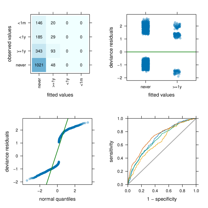
Figure 1: Diagnostic plots produced by plot(m): a confusion matrix (top left), deviance residuals against fitted.values (top right), qq-plot of the deviance residuals (bottom left), ROC curves for the four levels of the response variable.

and shown in Figure 1 suggest that the model is impacted by the imbalance between the number of people who have never used LSD and those who have (top-left panel). The ROC curves , computed one-versus-rest for each level of the response, are all similar and suggest that the model is an acceptable fit for the data (bottom-right panel). Running the standard 10 runs of 10-fold cross-validation suggested by Hastie et al. (2009), we confirm that neither precision nor recall are particularly high.

R> fairml.cv(response = r, sensitive = s, predictors = p, model = "fgrrm",+    unfairness = 0.05, method = "k-fold", k = 10, runs = 10,+    model.args = list(family = "multinomial", lambda = 0.1))

  k-fold cross-validation for fair models  model:                                      Fair Generalized Ridge Regression  number of folds:                       10  number of runs:                        10  average loss over the runs:    precision:                           0.6443056    recall:                              0.2144495  standard deviation of the loss:    precision:                           0.009535637    recall:                              0.006509704

This leaves us with two questions:

1. Does the fairness constraint have a strong impact on the goodness of fit and on the predictive performance of the model?

2. Would merging the levels of the response variable into a binary “used”/“never used” variable improve the model by making the data balanced?

We explore the answer to the first questions by plotting the profile of the estimated regression coefficients against the fairness constraint in Figure 2.

R> fairness.profile.plot(response = r, sensitive = s, predictors = p,+      model = "fgrrm", type = "coefficients",+      model.args = list(family = "multinomial", lambda = 0.1))

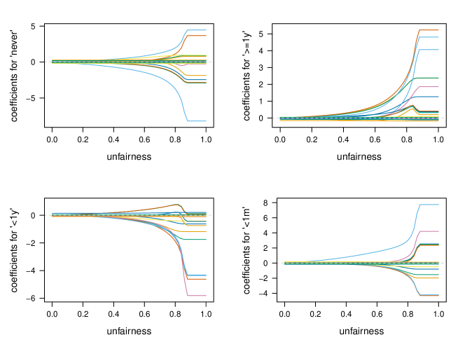
Figure 2: Profile plots for the regression coefficients as a function of the fairness constraint for all the levels of the response variable.

All regression coefficients are markedly shrunk towards zero for small values of unfairness: they take much larger values (in absolute value) when the model is unrestricted at unfairness equal to 1. This suggests that Age, Gender and Race are strongly associated with the predictors, in addition to their direct effect on the response. Their profiles flatten around unfairness equal to 0.85 which means that approximately 85% of the deviance of the model would be explained by the sensitive attributes when the fairness constraint becomes inactive.

As for re-balancing the response by transforming it into a binary variable,

R> levels(r) = c("never", "used", "used", "used")R> table(r)

rnever  used 1069   816 testing the predictive performance of the (no longer multinomial) FGRRM logistic regression model with cross-validation shows a sharp increase in recall and similar precision.

R> fairml.cv(response = r, sensitive = s, predictors = p, model = "fgrrm",+    unfairness = 0.05, method = "k-fold", k = 10, runs = 10,+    model.args = list(family = "binomial", lambda = 0.1))

  k-fold cross-validation for fair models  model:                                      Fair Generalized Ridge Regression  number of folds:                       10  number of runs:                        10  average loss over the runs:    precision:                           0.6866465    recall:                              0.5515931  standard deviation of the loss:    precision:                           0.002800798    recall:                              0.007156275 Therefore, we can conclude that the imbalance in the original response had a definite impact on the predictive accuracy of the multinomial FGRRM model.

5.2 Income and Labour Market

The National Longitudinal Survey data set contains the results of a survey from the U.S. Bureau of Labor Statistics to gather information on labour market activities (U.S. Bureau of Labor Statistics, 2023). Along with the incomes in 1990, 1996 and 2006 (income90, income96 and income06), the survey records the gender (gender), age (age) and race (race) of the respondents (our sensitive attributes), their physical characteristics (height, weight, general health), their criminal records (number of illegal acts and charges) and their level of education (grade90). As was the case in Section 5.1, we want to remove the bias introduced by the sensitive attributes through sampling bias and other mechanisms.

After loading the data, merging the levels of race and grade90 with low numbers of observations, and separating the response variable (income90 in this example), the predictors and the sensitive attributes,

R> data(national.longitudinal.survey)R> nlsy = national.longitudinal.surveyR> levels(nlsy$grade90)[1:5] = "7TH GRADE"R> levels(nlsy$race)[c(3, 14, 15)] = "CHINESE"R> r = nlsy[, "income90"]R> s = nlsy[, c("gender", "age", "race")]R> p = nlsy[, setdiff(names(nlsy),+               c("income90", "income96", "income06", "gender", "race", "age"))] we can fit an FRRM model (or equivalently a Gaussian FGRRM) as is commonly done in the literature (see, for instance, Komiyama et al., 2018).

R> m = frrm(response = r, sensitive = s, predictors = p, unfairness = 0.05)R> summary(m)

Fair Linear Regression ModelMethod: Fair Ridge RegressionCall:frrm(response = r, predictors = p, sensitive = s, unfairness = 0.05)Coefficients: (Intercept)  genderFemale           age     raceBLACK   raceCHINESE   1.6102737    -0.1873255     0.0186816    -0.0980725     0.0765317 [ reached getOption("max.print") -- omitted 62 entries ]Ridge penalty (sensitive attributes): 4.081 (predictors): 0Log-likelihood: -7835Residual standard error: 1.202Multiple R^2: 0.2337Komiyama’s R^2 (statistical parity): 0.05 with bound: 0.05 The $R^{2}$ coefficient reported by summary() suggests that the model is not a good fit for the data. Is this caused by the fairness constraint? Comparing the proportions of variance explained by the sensitive attributes and by the other predictors with fairness.profile.plot(), we can see in Figure 3 that without the fairness constraint (which becomes inactive at $r\approx 0.45$) the sensitive attributes explain nearly as much variability as the predictors.

R> fairness.profile.plot(response = r, sensitive = s, predictors = p,+      model = "frrm", type = "constraints", legend = TRUE)

Figure 3: Profile plot for the variance proportions explained by the decorrelated predictors and the sensitive attributes.

While removing or relaxing the fairness constraint would nearly double the $R^{2}$ of the model, the diagnostic plots produced by plot() (Figure 4) highlight two underlying issues with the data: higher incomes are truncated to $7.428$, which impacts the residuals in the right tail of the qq-plot and creates a pattern of points in the first two plots; and the response is bound below by zero.

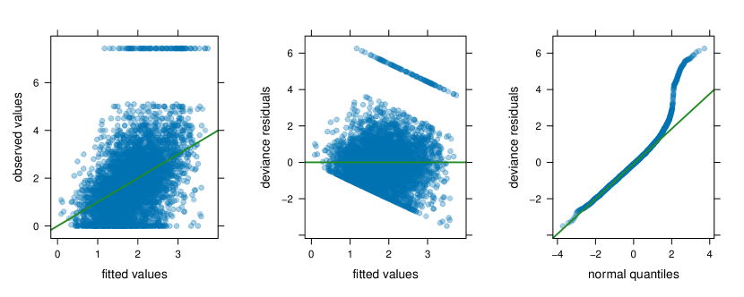
Figure 4: Diagnostic plots produced by plot() for an FGRRM model with a continuous response: observed versus fitted values (left), deviance residuals versus fitted values (centre) and a qq-plot of the deviance residuals (right).

To address them, we may consider removing the truncated observations and fitting a Poisson FGRRM model on the data, which is a natural choice for a non-negative response.

R> large.income = (r == max(r))R> table(large.income)

large.incomeFALSE  TRUE 4816    92

R> m = fgrrm(response = r[!large.income], sensitive = s[!large.income, ],+        predictors = p[!large.income, ], family = "poisson",+        unfairness = 0.05)

However, comparing the two models using cross-validation on the same data (and using the same folds) reveals that the original FRRM model appears to have better predictive accuracy for the chosen level of fairness than the Poisson FGRRM.

R> xval.lm =+    fairml.cv(response = r[!large.income], sensitive = s[!large.income, ],+      predictors = p[!large.income, ], model = "frrm", unfairness = 0.05,+      method = "k-fold", k = 10, runs = 10)R> xval.glm =+    fairml.cv(response = r[!large.income], sensitive = s[!large.income, ],+      predictors = p[!large.income, ], model = "fgrrm", unfairness = 0.05,+      model.args = list(family = "poisson"), method = "custom-folds",+      folds = cv.folds(xval.lm))R> summary(cv.loss(xval.lm))

   Min. 1st Qu.  Median    Mean 3rd Qu.    Max. 0.9908  0.9929  0.9937  0.9938  0.9950  0.9967

R> summary(cv.loss(xval.glm))

   Min. 1st Qu.  Median    Mean 3rd Qu.    Max.  1.128   1.130   1.131   1.131   1.133   1.134

The other two models implemented in fairml, zlm() from Zafar et al. (2019) and nclm() from Komiyama et al. (2018), also appear to fit the data less well than FRRM.

R> m2 = nclm(response = r[!large.income], sensitive = s[!large.income, ],+         predictors = p[!large.income, ], unfairness = 0.05)

Loading required namespace: cccp

R> m3 = zlm(response = r[!large.income], sensitive = s[!large.income, ],+         predictors = p[!large.income, ], unfairness = 0.05)

Loading required namespace: CVXR

R> summary(m2)

Fair Linear Regression ModelMethod: Komiyama et al. (2018)Call:nclm(response = r[!large.income], predictors = p[!large.income,    ], sensitive = s[!large.income, ], unfairness = 0.05)Coefficients: (Intercept)  genderFemale           age     raceBLACK   raceCHINESE   1.4635456    -0.1974729     0.0162676     0.0076029     0.2002531 [ reached getOption("max.print") -- omitted 62 entries ]Ridge penalty: 0Custom covariance matrix: FALSELog-likelihood: -6757Residual standard error: 0.9912Multiple R^2: 0.248Komiyama’s R^2 (statistical parity): 0.04984 with bound: 0.05

R> summary(m3)

Fair Linear Regression ModelMethod: Zafar’s Linear RegressionCall:zlm(response = r[!large.income], predictors = p[!large.income,    ], sensitive = s[!large.income, ], unfairness = 0.05)Coefficients:(Intercept)    grade90.L    grade90.Q    grade90.C    grade90.4  1.4581758    1.3300355    0.0028437   -0.2713558    0.0125724 [ reached getOption("max.print") -- omitted 34 entries ]Log-likelihood: -6940Residual standard error: 1.027Multiple R^2: 0.1887Marginal correlation (disparate impact):genderFemale          age    raceBLACK  raceCHINESE  raceENGLISH    0.032564     0.007244     0.036622     0.013714     0.041502 [ reached getOption("max.print") -- omitted 23 entries ]with bound: 0.05

Therefore, we can conclude that FRRM fits the data best at unfairness = 0.05 among the models we have examined.

5.3 Using Different Fairness Constraints

The last feature of fairml we will showcase is the ability to plug custom mathematical characterisations of fairness into frrm() and fgrrm(). Built-in fairness definitions are identified by the labels listed in Table 2. Custom definitions can be provided as functions with signature function(model, y, S, U, family) where model is the model whose fairness we are evaluating, family is the GLM family the model belongs to, and y, S, U are $\mathbf{y},\mathbf{S},\mathbf{U}$ from (3). With the help of str() and a dummy function, we can see that the model object contains several key quantities describing the model we are evaluating.

R> dummy.fairness =+    function(model, y, S, U, family) { str(model); return(c(value = 0)) }R>R> m = fgrrm(response = r, sensitive = s, predictors = p, unfairness = 0.05,+        definition = dummy.fairness, family = "gaussian")

List of 5 $ coefficients: Named num [1:67] 0.6526 -0.7423 0.0754 -0.0635 0.4791 ...  ..- attr(*, "names")= chr [1:67] "(Intercept)" "genderFemale" "age" ... $ deviance    : num 6350 $ loglik      :Class ’logLik’ : -7596 (df=68) $ fitted      : num [1:4908] 1.86 2.92 1.63 2.32 3.5 ... $ residuals   : num [1:4908] 0.1419 -0.6214 0.0683 0.6846 0.5017 ...

The only requirement for this function is that it should return an array with an element named "value" that takes a value between 0 (perfect fairness) and 1 (no constraint). Built-in functions return additional elements that are then used in fairness.profile.plot(), but any element other than that named "value" will be ignored for custom fairness definitions. So, for instance, we can define fairness as a weighted mean of statistical parity and individual fairness like Berk et al. (2017) did by reusing the internal functions that fairml uses to estimate them.

R> combined.fairness = function(model, y, S, U, family) {++    value =+      0.4 * fairml:::fgrrm.sp.komiyama(model, y, S, U, family)[["value"]] ++      0.6 * fairml:::fgrrm.if.berk(model, y, S, U, family)[["value"]]++    return(c(value = value))++  }#COMBINED.FAIRNESS

Or we can implement a completely different definition of fairness, such as a bound on the correlation between fitted values and sensitive attributes in the spirit of Zafar et al. (2019).

R> custom.fairness =+    function(model, y, S, U, family)+      return(c(value = max(abs(cor(model$fitted, S)))))

Or, assuming we only have a single binary sensitive attribute in the data, we can bound the p-value of a Kolmogorov-Smirnov test between the distributions of the fitted values for the two groups identified by the sensitive attribute.

R> custom.fairness = function(model, y, S, U, family) {++    group1 = model$fitted[S == 0]+    group2 = model$fitted[S == 1]+    value = ks.test(group1, group2)$p.value++    return(c(value = value))++  }#CUSTOM.FAIRNESS

In essence, the information provided in the arguments to the custom function combined with the functionality of other R packages allows for a great deal of flexibility.

6 Summary and Discussion

Algorithmic fairness is a topic with important practical applications and a quickly-evolving research field. The core of the fairml package is our previous work in Scutari et al. (2022), which separates the estimation of a fair linear model from the mathematical characterisation of fairness. On the one hand, this modular design choice allows for a compact implementation that supports all GLM families which makes fairml useful in a variety of application fields. On the other hand, the ability to plug any definition of fairness in the model without having to reimplement model estimation as well is a valuable asset in research. Furthermore, fairml produces models whose statistical properties and best practices are well known (as opposed to the black-box estimators based on numerical optimisers that make up most of the literature) and provides the standard tools to validate and evaluate them.

References

- Agarwal et al. (2018) Agarwal A, Beygelzimer A, Dudik M, et al. (2018). “A Reductions Approach to Fair Classification.” Proceedings of Machine Learning Research, 80, 60–69. 35th International Conference on Machine Learning (ICML).
- Agarwal et al. (2019) Agarwal A, Dudik M, Wu ZS (2019). “Fair Regression: Quantitative Definitions and Reduction-Based Algorithms.” Proceedings of Machine Learning Research, 97, 120–129. 36th International Conference on Machine Learning.
- Angwin et al. (2016) Angwin J, Larson J, Mattu S, Kirchner L (2016). Machine Bias: There’s Software Used Across the Country to Predict Future Criminals. And It’s Biased Against Blacks. ProPublica. URL https://www.propublica.org/article/machine-bias-riskassessments-in-criminal-sentencing.
- Barredo Arrieta et al. (2020) Barredo Arrieta A, Díaz-Rodríguez N, Del Ser J, et al. (2020). “Explainable Artificial Intelligence (XAI): Concepts, Taxonomies, Opportunities and Challenges Toward Responsible AI.” Information Fusion, 58, 82–115.
- Bellamy et al. (2019) Bellamy RKE, Dey K, Hind M, et al. (2019). “AI Fairness 360: An Extensible Toolkit for Detecting and Mitigating Algorithmic Bias.” IBM Journal of Research and Development, 63(4/5), 1–15. 10.1147/JRD.2019.2942287.
- Berk et al. (2017) Berk R, Heidari H, Jabbari S, et al. (2017). “A Convex Framework for Fair Regression.” In Fairness, Accountability, and Transparency in Machine Learning (FATML).
- Berk et al. (2021) Berk R, Heidari H, Jabbari S, et al. (2021). “Fairness in Criminal Justice Risk Assessments: The State of the Art.” Sociological Methods & Research, 50(1), 3–44. 10.1177/0049124118782533.
- Calders et al. (2013) Calders T, Karim A, Kamiran F, et al. (2013). “Controlling Attribute Effect in Linear Regression.” In Proceedings of the 13th IEEE International Conference on Data Mining, pp. 71–80. 10.1109/ICDM.2013.114.
- Calmon et al. (2017) Calmon F, Wei D, Vinzamuri B, et al. (2017). “Optimized Pre-Processing for Discrimination Prevention.” In Advances in Neural Information Processing Systems, volume 30, pp. 3992–4001.
- Cath et al. (2018) Cath C, Wachter S, Mittelstadt B, et al. (2018). “Artificial Intelligence and the ‘Good Society’: the US, EU, and UK Approach.” Science and Engineering Ethics, 24(2), 505–528. 10.1007/s11948-017-9901-7.
- Choraś et al. (2020) Choraś M, Pawlicki M, Puchalski D, Kozik R (2020). “Machine Learning—The Results Are Not the only Thing that Matters! What About Security, Explainability and Fairness?” In Proceedings of the International Conference on Computational Science (ICCS), pp. 615–628. 10.1007/978-3-030-50423-6_46.
- Chzhen et al. (2020) Chzhen E, Denis C, Hebiri M, et al. (2020). “Fair Regression via Plug-In Estimator and Recalibration with Statistical Guarantees.” In Advances in Neural Information Processing Systems, volume 33, pp. 19137–19148.
- Cotter et al. (2019) Cotter A, Gupta M, Jiang H, et al. (2019). “Training Well-Generalizing Classifiers for Fairness Metrics and Other Data-Dependent Constraints.” Proceedings of Machine Learning Research, 97, 1397–1405. 36th International Conference on Machine Learning.
- D’Alessandro et al. (2017) D’Alessandro B, O’Neil C, LaGatta T (2017). “Conscientious Classification: A Data Scientist’s Guide to Discrimination-Aware Classification.” Big Data, 5(2), 120–134. 10.1089/big.2016.0048.
- de B. G. de Oliveira et al. (2021) de B G de Oliveira T, Vieira LP, Silva GRL, et al. (2021). \pkgpredfairness: Discrimination Mitigation for Machine Learning Models. URL https://cran.r-project.org/package=predfairness.
- Del Barrio et al. (2020) Del Barrio E, Gordaliza P, Loubes JM (2020). Review of Mathematical Frameworks for Fairness in Machine Learning. URL https://arxiv.org/abs/2005.13755.
- Díaz et al. (2019) Díaz M, Johnson I, Lazar A, et al. (2019). “Addressing Age-Related Bias in Sentiment Analysis.” In Proceedings of the Twenty-Eighth International Joint Conference on Artificial Intelligence, pp. 6146–6150. 10.24963/ijcai.2019/852.
- Do et al. (2022) Do H, Putzel P, Martin AS, et al. (2022). “Fair Generalized Linear Models with a Convex Penalty.” Proceedings of Machine Learning Research, 162, 5286–5308. 39th International Conference on Machine Learning.
- Dua and Graff (2023) Dua D, Graff C (2023). UCI Machine learning repository. University of California, School of Information and Computer Science. URL https://archive.ics.uci.edu/ml/.
- European Commission (2021) European Commission (2021). Proposal for a Regulation Laying Down Harmonised Rules on Artificial Intelligence. URL https://digital-strategy.ec.europa.eu/en/library/proposal-regulation-laying-down-harmonised-rules-artificial-intelligence.
- Fehrman et al. (2017) Fehrman E, Muhammad AK, Mirkes EM, et al. (2017). “The Five Factor Model of Personality and Evaluation of Drug Consumption Risk.” In Data Science, pp. 231–242. 10.1007/978-3-319-55723-6_18.
- Friedman et al. (2010) Friedman J, Hastie T, Tibshirani R (2010). “Regularization Paths for Generalized Linear Models via Coordinate Descent.” Journal of Statistical Software, 33(1), 1–22. 10.18637/jss.v033.i01.
- Fu et al. (2020) Fu A, Narasimhan B, Boyd S (2020). “\pkgCVXR: An R Package for Disciplined Convex Optimization.” Journal of Statistical Software, 94(14), 1–34. 10.18637/jss.v094.i14.
- Fukuchi et al. (2013) Fukuchi K, Sakuma J, Kamishima T (2013). “Prediction with Model-Based Neutrality.” In Proceedings of the Joint European Conference on Machine Learning and Knowledge Discovery in Databases (ECML PKDD), pp. 499–514. Springer. 10.1587/transinf.2014EDP7367.
- Fuster et al. (2022) Fuster A, Goldsmith-Pinkham P, Ramadorai T, Walther A (2022). “Predictably Unequal? The Effects of Machine Learning on Credit Markets.” The Journal of Finance, 77(1), 5–47. 10.1111/jofi.13090.
- Hardt et al. (2016) Hardt M, Priceric E, Srebro N (2016). “Equality of Opportunity in Supervised Learning.” In Advances in Neural Information Processing Systems, volume 29, pp. 3315–3323.
- Hastie et al. (2009) Hastie T, Tibshirani R, Friedman J (2009). The Elements of Statistical Learning: Data Mining, Inference, and Prediction. 2nd edition. Springer. 10.1007/978-0-387-84858-7.
- Hort and Sarro (2022) Hort M, Sarro F (2022). “Privileged and Unprivileged Groups: An Empirical Study on the Impact of the Age Attribute on Fairness.” In Proceedings of the International Workshop on Equitable Data and Technology, pp. 17–24. 10.1145/3524491.3527308.
- Komiyama et al. (2018) Komiyama J, Takeda A, Honda J, Shimao H (2018). “Nonconvex Optimization for Regression with Fairness Constraints.” Proceedings of Machine Learning Research, 80, 2737–2746. 35th International Conference on Machine Learning.
- Kozodoi and Varga (2021) Kozodoi N, Varga TV (2021). \pkgfairness: Algorithmic Fairness Metrics. URL https://cran.r-project.org/package=fairness.
- Lambrecht and Tucker (2019) Lambrecht A, Tucker C (2019). “Algorithmic Bias? An Empirical Study of Apparent Gender-Based Discrimination in the Display of STEM Career Ads.” Management Science, 65(7), 2966–2981. 10.1287/mnsc.2018.3093.
- Lang et al. (2019) Lang M, Binder M, Richter J, et al. (2019). “mlr3: A Modern Object-Oriented Machine Learning Framework in R.” Journal of Open Source Software, 4(44), 1903. 10.21105/joss.01903.
- Lohr (2021) Lohr SL (2021). Sampling: Design and Analysis. 3rd edition. CRC Press. 10.1201/9780429298899.
- Mehrabi et al. (2021) Mehrabi N, Morstatter F, Saxena N, et al. (2021). “A Survey on Bias and Fairness in Machine Learning.” ACM Computing Surveys, 54(6), 115. 10.1145/3457607.
- Narasimhan (2018) Narasimhan H (2018). “Learning with Complex Loss Functions and Constraints.” Proceedings of Machine Learning Research, 84, 1646–1654. 21st International Conference on Artificial Intelligence and Statistics.
- Pérez-Suay et al. (2017) Pérez-Suay A, Laparra V, Mateo-García G, et al. (2017). “Fair Kernel Learning.” In Proceedings of the Joint European Conference on Machine Learning and Knowledge Discovery in Databases (ECML PKDD), pp. 339–355. Springer. 10.1007/978-3-319-71249-9_21.
- Pessach and Shmueli (2022) Pessach D, Shmueli E (2022). “A Review on Fairness in Machine Learning.” ACM Computing Surveys, 55(3), 51. 10.1145/3494672.
- Pfaff (2022) Pfaff B (2022). \pkgcccp: Cone Constrained Convex Problems. URL https://cran.r-project.org/package=cccp.
- Pfisterer et al. (2022) Pfisterer F, Siyi W, Lang M (2022). \pkgmlr3fairness: Fairness Auditing and Debiasing for \pkgmlr3. https://mlr3fairness.mlr-org.com, https://github.com/mlr-org/mlr3fairness.
- R Core Team (2022) R Core Team (2022). R: A Language and Environment for Statistical Computing. R Foundation for Statistical Computing, Vienna, Austria. URL https://www.R-project.org/.
- Raghavan et al. (2020) Raghavan M, Barocas S, Kleinberg J, Levy K (2020). “Mitigating Bias in Algorithmic Hiring: Evaluating Claims and Practices.” In Proceedings of the 3rd Conference on Fairness, Accountability and Transparency, pp. 469–481. 10.1145/3351095.3372828.
- Schafer et al. (2021) Schafer J, Opgen-Rhein R, Zuber V, et al. (2021). \pkgcorpcor: Efficient Estimation of Covariance and (Partial) Correlation. URL https://cran.r-project.org/package=corpcor.
- Scutari (2022) Scutari M (2022). \pkgfairml: Fair Models in Machine Learning. URL https://cran.r-project.org/package=fairml.
- Scutari et al. (2022) Scutari M, Panero F, Proissl M (2022). “Achieving Fairness with a Simple Ridge Penalty.” Statistics and Computing, 32, 77. 10.1007/s11222-022-10143-w.
- Simon et al. (2011) Simon N, Friedman J, Hastie T, Tibshirani R (2011). “Regularization Paths for Cox’s Proportional Hazards Model via Coordinate Descent.” Journal of Statistical Software, 39(5), 1–13. 10.18637/jss.v039.i05.
- Tay et al. (2023) Tay JK, Narasimhan B, Hastie T (2023). “Elastic Net Regularization Paths for All Generalized Linear Models.” Journal of Statistical Software, 106(1), 1–31. 10.18637/jss.v106.i01.
- Tolan et al. (2019) Tolan S, Miron M, Gómez E, Castillo C (2019). “Why Machine Learning May Lead to Unfairness.” In Proceedings of the Seventeenth International Conference on Artificial Intelligence and Law, pp. 83–92. 10.1145/3322640.3326705.
- United Nations (2015) United Nations (2015). Sustainable Development Goals: The Sustainable Development Agenda. URL https://www.un.org/sustainabledevelopment/development-agenda/.
- United Nations (2023) United Nations (2023). AI for Good. URL https://aiforgood.itu.int/.
- U.S. Bureau of Labor Statistics (2023) US Bureau of Labor Statistics (2023). National Longitudinal Surveys of Youth Data Set. URL https://www.bls.gov/nls/.
- Wiśniewski and Biecek (2022) Wiśniewski J, Biecek P (2022). “\pkgfairmodels: a Flexible Tool for Bias Detection, Visualization, and Mitigation in Binary Classification Models.” The R Journal, 14, 227–243. 10.32614/RJ-2022-019.
- Woodworth et al. (2017) Woodworth B, Gunasekar S, Ohannessian MI, Srebro N (2017). “Learning Non-Discriminatory Predictors.” Proceedings of Machine Learning Research, 65, 1920–1953. Conference on Learning Theory.
- Zafar et al. (2019) Zafar MB, Valera I, Gomez-Rodriguez M, Gummadi KP (2019). “Fairness Constraints: a Flexible Approach for Fair Classification.” Journal of Machine Learning Research, 20, 1–42.