Semi-Parametric Identification and Estimation of Interaction and Effect Modification in Mixed Exposures using Stochastic Interventions

Abstract

In many fields, including environmental epidemiology and medicine, researchers strive to understand the joint impact of a mixture of exposures or treatments. This involves analyzing a vector of exposures or treatments rather than a single exposure, with the most significant individual exposures and exposure sets being unknown. Examining every possible interaction or effect modification in a high-dimensional vector of candidates can be challenging or even impossible. To address this challenge, we propose a method for the automatic identification and estimation of individual exposures in a mixture with explanatory power, baseline covariates that modify the impact of a mixture exposure or set of mixture variables, and sets of mixture exposures that have synergistic non-additive relationships. We define these parameters in a realistic nonparametric statistical model and use data-adaptive machine learning methods to identify these variables and variable sets while estimating the nuisance parameters for our target parameters of interest to avoid model misspecification. We establish a prespecified target parameter applied to variable sets when identified and use cross-validation procedures to train efficient estimators employing targeted maximum likelihood estimation for our target parameter given these sets. Our approach applies a shift intervention targeting individual variable importance, interaction, and effect modification based on the data-adaptively determined sets of variables. Our methodology is implemented in the open-source SuperNOVA package in R, enabling researchers to discover interaction and effect modification in a mixed exposure, providing robust statistical inference for these estimands without relying on arbitrary parametric assumptions. Our approach has broad applications across various fields and holds the potential to significantly advance our understanding of complex mixtures of exposures. We demonstrate the utility of our method through simulations, showing that our estimator is efficient and asymptotically linear under conditions requiring $n^{1/4}$-consistency of certain regression functions. We apply our method to the National Institute of Environmental Health Science mixtures workshop data, revealing correct identification of antagonistic and agonistic interactions built into the data. Additionally, we investigate the association between exposure to persistent organic pollutants and longer leukocyte telomere length and compare findings to previous results using other mixture methods.

Keywords Stochastic Interventions  $\cdot$ Causal Inference  $\cdot$ Targeted Learning  $\cdot$ Interaction

1 Introduction

Individual health outcomes are influenced by the complex interplay of our environment and biology. We are exposed to multiple pollutants simultaneously, such as air pollution and contaminants in water. As a result, we should expect complex relationships to exist between these exposures, where certain exposures synergize to create super-additive effects on outcomes, and others antagonize or nullify the effects of exposure. Despite this, most epidemiological studies have focused on analyzing one pollutant at a time Meng et al. (2021); wan ; Xiao et al. (2021), partly due to the reliance on traditional generalized linear models (GLMs) that estimate each mixture component after controlling for others Bauer et al. (2020); García-Villarino et al. (2022); Zhang et al. (2019). Such models are inadequate for accurately modeling complex multi-pollutant mixtures and understanding their relationships. The inadequacy of the use of parametric models to efficiently explore the space of possible interactions is a significant limitation in environmental exposure data analysis. Traditional methods, such as parametric models, struggle to capture complex relationships due to their rigid assumptions and constrained structure. GLMs attempt to model complex effects; however, their constrained nature restricts their ability to accurately represent the true underlying relationships. Furthermore, alternative approaches like tree-based methods do not provide explicit estimators of interactions, limiting their utility in deciphering intricate relationships between various factors. Consequently, there is a growing need for more flexible and adaptive methods that can better capture the intricacies of environmental exposure data, allowing for a more comprehensive understanding of the potential causal relationships and interactions at play.

In the context of analyzing mixture data using GLMs, it is critical to consider the limitations of this modeling approach. Mixture data is often characterized by high-dimensionality, multicollinearity, nonlinearity, and complex interactions among exposures. These features are well-established in the literature Cao et al. (2021); Wang et al. (2020); Xu et al. (2021); Billionnet et al. (2011). When applying GLMs to such data, the analyst is essentially imposing a linear function on a non-linear relationship, which raises important questions about the interpretation of the resulting model coefficients. Specifically, what is the meaning of the beta coefficients obtained from this linear projection, and is there any utility in interpreting the coefficients in the presence of non-linearity and interactions? Furthermore, when estimating the joint impact of co-exposures, does it make sense to simply add up the coefficients obtained from the GLM, such as what is done in weighted quantile sum regression? These are important considerations that we address in this study as we introduce a new statistical method for analyzing mixture data.

In order to derive meaningful interpretations from statistical quantities, it is important to begin by framing the research question as a causal one. For example, when considering the impact of mixed exposures to persistent organic pollutants, the relevant questions may involve the effect of a specific dioxin level on leukocyte telomere length, the difference in leukocyte telomere length between individuals exposed to dioxin levels above and below EPA regulations, or the combined effect of increases in dioxin and polychlorinated biphenyl (PCB) exposure on leukocyte telomere length. To answer these questions, it is necessary to use estimators that make minimal assumptions and can capture the underlying functional forms, including interactions and nonlinearity, of the mixture data. This requires the use of flexible algorithms to avoid unrealistic linear assumptions.

Analysts faced with high-dimensional and multicollinear exposure data often turn to methods like principal component analysis (PCA) Zhou et al. (2016); Roberts and Martin (2006) or penalized regression Navas-Acien et al. (2021); Xin Wang, Bhramar Mukherjee and Park (2018); Yitshak-Sade et al. (2020); McEligot et al. (2020) to address these challenges. PCA produces a set of linearly uncorrelated variables that represent combinations of the original exposures, and these are then used as predictors in a linear model. Penalized regression models, such as least absolute shrinkage and selection operator (LASSO) or Ridge regression, can actively select a smaller set of exposures from the full exposure profile, based on the strength of their associations with the outcome. While these methods can help with issues of multicollinearity and high-dimensionality, the resulting quantities are often not easily interpretable in the context of causal questions that is informative for chemical regulation and public policy. For example, with PCA, it can be difficult to link the resulting principal components to specific exposures, and it may not be clear how the outcome changes with an increase in a particular exposure. Similarly, with penalized regression models, the selected subset of exposures may not represent a causal set, and interpreting the resulting coefficients may not be straightforward given the penalization imposed. Another popular approach in mixed exposure analysis involves: 1) reducing dimensionality through a technique such as PCA, 2) using a regression model on the reduced set of variables, 3) summing up the coefficients to estimate the joint effect of the mixture, and 4) possibly using Bayesian kernal machine regression (BKMR) to assess for nonlinearity/interaction. However, given evidence of nonlinearity and interaction found in many studies using the more flexible BKMR model, the question remains on how to interpret individual or summed coefficients in a misspecified linear model, and how these results address the proposed questions about mixed exposure.

In general, researchers need methods based on modified treatment policies. That is, methods that allow understanding of how various health related outcomes change given a change in exposure where the interventions go through a model that most accurately captures the underlying functional forms of the data. Therefore, the field needs non-parametric definitions for marginal effects, interaction and effect modification based on modified treatment policies. These estimates would provide answers for questions such as 1. what is the joint impact of multiple exposures on an outcome, 2. how does the joint impact of co-exposure compare to individual exposure (interaction)? and 3. is there heterogeneity in the impact of joint exposure/interaction across different subpopulations of individuals?. In each of these cases we need the target parameter to be defined outside considerations of the statistical model being used. For example, traditionally it has been taught that to assess for interaction to simply include an interaction term in a GLM. Of course, this is assessing for a multiplicative interaction between (normally) two exposures in a projected linear model with only main terms for the remaining exposures and covariates. Give there is likely nonlinearity in the exposures and covariates with possible interactions between both, once again we ask what does multiplying two exposures and estimating the coefficient of this term mean in a misspecified linear model? Furthermore, effect modification and interaction are measured in the same way with GLMs. Within the context of linear models, there is no statistical distinction between interaction and effect modification. The difference arises from interpreting the interaction term used in the regression. However, within the non-parametric counterfactual framework these target parameters are different. Interaction is defined as the effects given an intervention on two or more exposures whereas effect modification is defined as the effect of one intervention varying across strata of a second unperturbed variable. Vanderweele (2009). If we consider two binary exposures, with observations defined as $O=(W,A,Y)$ where $W$ are covariates, $A$ is a binary exposure and $Y$ is the outcome, we might define interaction in a mixture as the causal target parameter $E[E[Y|A_{1}=1,A_{2}=1|W]-[E[Y|A_{1}=1,A_{2}=0|W]-E[Y|A_{1}=0,A_{2}=1|W]]+E[Y|A_{1}=0,A_{2}=0|W]]$ which in the first term states we are taking the whole population and forcing individuals to be exposed to both exposures, the second forcing individuals to be exposed to $A_{1}$ and not $A_{2}$, the third term forcing individuals to be exposed to $A_{2}$ but not $A_{1}$ and the fourth term forcing individuals to not be exposed to $A_{1}$ or $A_{2}$. By subtracting the individual exposures from the joint we can estimate the greater impact a joint exposure has on the outcome. For such a target parameter we would then show that we can construct an unbiased and maximally efficient estimator under certain causal assumptions (i.e. no unmeasured confounding), but without imposing additional modeling assumptions. Targeted maximum likelihood and efficient estimating equations are two “recipes” for constructing such estimators that we could apply in this setting van der Laan and Rose (2011, 2018) Glynn and Quinn (2009).

Of course, in most studies the mixture data is not composed of two binary exposures. Our target parameter should be able to handle a variety of data types (binary, multinomial, continuous) and many exposures. For a continuous exposure, there is no pathwise differentiable dose-response parameter in a nonparametric model. However, we can use stochastic exposure regimes, or stochastic interventions, which replaces $f_{A}$, a function that gives rise to the exposure $A$, and $g(A\mid W)$, the natural conditional density of $A$ given covariates $W$, with a candidate density $g_{A_{\delta}}(A\mid W)$. More simply, we could replace the observed probability density distribution of, say, persistant organic pollutant (POP) exposure with that of a distribution if everyone were exposed an additional 1 pg/g unit. Because we are interested in the change in probability density, this approach works for all data-types and easily extends to multiple exposures, for example, observing how the joint density changes given an increase in a dioxin and furan, which were exposures of interest in mixture analysis workshops to study impacts on longer telomere length Mitro et al. (2016). Using $d_{x}(A_{x})$ notation to denote a shift in an exposures conditional density distribution, we can extend the original definition of interaction under joint binary intervention to: $E[Y(d_{1}(A1),d_{2}(A2)]-[E[Y(d_{1}(A1),A2)]+E[Y(A1,d_{2}(A2))]$ where now we are forcing the whole population to experience a shift in exposure(s) $A_{x}$ for some shift $\delta$. This is simply comparing the outcome under joint exposure shifts to the sum of individual shifts. This provides a non-parametric definition of interaction that is not dependent on a particular estimator.

The same limitations to binary treatment also exists in methods for estimating the heterogeneous treatment/exposure effects. One approach to estimating heterogenous treatment effects is through looking at the average treatment effect (ATE) within a specific subgroup of the population defined by a set of covariates, this is known as the conditional average treatment effect (CATE). In the context of environmental health and mixed exposures, estimation of heterogenous exposure effects can help identify vulnerable populations that are differentially impacted by certain exposures or groups of exposures. These effects are typically associated with exposure effect modifiers (EEMs), which are covariates that modify the association of exposure on the outcome. Traditional parametric methods, such as GLMs, can detect EEMs under stringent conditions about the data-generating process, but when the posited functional relationship does not correspond to reality, inference is invalid. Detecting interactions in data involves a data-adaptive approach, which when relying on regression techniques, involves exploring various combinations of main effects and their tensor products. This process can involve trying different polynomial terms, interaction terms, and other transformations of the predictor variables to capture the complexity of the relationships between them. However, the resulting parameters reported from such an approach are heavily dependent on the model selection process.

More flexible semi-parametric methods have been developed and are described here Künzel et al. (2019). However, the metaalgorithms discussed in this paper, such as the T-learner and S-learner, are limited to only binary treatment. The T-learner is a machine learning approach for estimating the CATE, which involves training separate prediction models on treated and control groups and then calculating the difference in their predictions for individual observations. The S-learner is a machine learning approach for estimating the CATE, which involves training a single prediction model on the entire dataset with treatment as an additional covariate and then calculating the difference in predictions with and without treatment for individual observations. While some researchers estimate heterogeneous treatment effects by analyzing ATEs for meaningful subgroups or using causal forests Wager and Athey (2018), Künzel et al. (2019) propose a new metaalgorithm, the X-learner, which builds on the T-learner and uses observed outcomes to estimate unobserved individual treatment effects. This involves training separate prediction models for treated and control groups, estimating individual treatment effects using both models, and then using a third model to learn the relationship between covariates and these estimated treatment effects to make individualized predictions. However, it is important to note that the T-, S-, and X-learners may not be suitable for estimating the CATE in the context of environmental exposures, where most chemicals are continuous, and alternative methods are needed.

Our approach is to investigate how the conditional average treatment effect for various stochastic shift interventions is different for certain vulnerable populations as an estimation strategy for effect modification. To do this, we can use an a priori specified estimator to find regions in the covariate space that best explain variance in the conditional treatment effects. That is, we simply regress the vector of expected individual counterfactual differences under a shift intervention onto the the covariates space using the optimal decision tree to identify interpretable regions that explain variability in the conditional average treatment effect. This approach then provides a semi-parametric definition of effect modification.

The problem only gets more complicated in mixtures. Non-parametric estimation of main effects, interactions, effect modification, and mediation for a continuous mixture of exposures (with more than two components), high-dimensional baseline covariates, and intermediates is impossible without large sample sizes. As discussed, existing methods reduce the dimension of the problem artificially by imposing highly constrained models, resulting in biased estimations. No method currently exists to simultaneously estimate all these estimands motivated by causal parameters. Given these limitations, it is impossible to reduce the problem’s dimension non-data-adaptively. Therefore, it is necessary to use the data both to define the specific parameters of interest and to estimate the data-adaptively defined parameters, which is an unavoidable part of the estimation problem. Addressing this issue with simplified models is not a viable solution.

Recent developments in both data-adaptive parameters and new estimators for the impact of relevant interventions on continuous exposures have paved the way for methodological research advancements. The goal of this paper is to develop an estimation machine that, under highly flexible (optimal) estimates of the data-generating distribution, can both identify which potential causal parameters have support in the data and use cross-validated targeted minimum loss-based estimation (CV-TMLE) to estimate and provide inference about them without overfitting. This approach will allow for a more accurate and unbiased analysis of the complex relationships in environmental exposure data. Furthermore, these estimates must be interpretable using modified treatment policies.

Identifying these relationships and estimating the target parameter is challenging, as both cannot be achieved using the same data without bias. To address this, sample splitting is necessary where one part of the data is used to identify the variable relationships, while the other is used to estimate the target parameters. We need a data-driven search of exposure space to find the sub-spaces that, the change of which, result in the largest change in the outcome, in a very large statistical model capable of capturing very complex relationships. To do this, we propose using an ensemble of basis spline models and selecting the best one. With this best fitting model, which is a linear combination of basis functions, we propose a nonparametric way to do ANOVA. This is analogies to a simple type III ANOVA and generalizes to big statistical models with joint exposures. Bases with interaction and effect modification variables that meet a specific F-statistic threshold are used to estimate the target parameters in the estimation data.

Our proposed method called SuperNOVA uses data-adaptive parameters Hubbard et al. (2016) and cross-validated targeted minimum loss-based estimation (CV-TMLE) Zheng and van der Laan (2010), resulting in a powerful approach for estimating the joint impact, interaction, and effect modification of a mixed exposure. By using CV-TMLE our estimates are guaranteed to have consistency, efficiency, and multiple robustness despite using highly flexible learners (ensemble machine learning) estimate a data-adaptive parameters. Data-adaptive parameters refer to parameters of interest that are identified and estimated through a data-driven process, in our case, the exposures are identified and a stochastic shift in these variables are estimated using the observed data. SuperNOVA is a statistical method that estimates the adjusted joint total impacts of multivariate exposures by searching for the sub-spaces that are "most important" for the outcome. This method generalizes associations away from discretized exposures to interpretable parameters that can handle continuous joint exposures. SuperNOVA has a built-in data-adaptive way for both estimation and parameter-generation to optimize for "complexity," and is capable of modeling complex nonlinear functions while still being able to fit simpler models if supported by the data. The method estimates interactions using a combination of shift interventions among the subspaces of joint exposures found in the parameter-generating part and can also estimate effect modification for particular covariates data-adaptively identified. Additionally, SuperNOVA provides marginal impacts of shift exposures for the relevant subset of them determined in the parameter-generating part and provides robust inference despite using the data to both define the parameter and estimate it using CV-TMLE.

This manuscript is organized as follows, in Section 2.1 we give a background of semi-parametric methodology for stochastic interventions, in section 2.2 we discuss the target parameter for interaction given a fixed set of variables and in 2.3 we describe the effect modification parameter under a fixed set of variables, 2.4 describes assumptions necessary for our statistical estimates to have a causal interpretation. In section 3.1 we discuss estimation and inference of the interaction for a fixed variable set. In 3.2 we discuss estimation of the effect modification for a fixed variable set. In section 4 we discuss data-adaptively determining the variable set. In section 5 we show how this requires cross-estimation which builds from 2.2 for a fixed variable set. In section 5 we expand this to cross-estimation to k-fold CV and discuss methods for pooling estimates across the folds. Lastly, in section 5.3, because we may data-adaptively choose different deltas (when the choice of shift is also data-adaptively determined) across the folds and different variable sets chosen across the CV folds, we discuss the pooled estimates across the folds. In section 6 we discuss simulations of interactions and effect modification and show our estimates are asymptotically unbiased with normal sampling distributions. In section 7 we apply SuperNOVA to the NIEHS mixtures workshop data and identify interactions built into the synthetic data. In section 7.1 we compare SuperNOVA to exising mixture methods. In section 7.2 we apply SuperNOVA to NHANES data to determine if there is association between mixed POPs and leukocyte telomere length. Section 8 describes our SuperNOVA software. We end with a brief discussion of the SuperNOVA method in Section 9.

2 The Estimation Problem

2.1 Setup and Notation

Our setting is an observational study with baseline covariates ($W\in\mathbb{R}^{p}$), multiple exposures ($A\in\mathbb{R}^{m}$), and a single-timepoint outcome ($Y$). Let $O=(W,A,Y)$ denote the observable data. We use $P_{0}$ to denote the data-generating distribution. That is, each sample from $P_{0}$ results in a different realization of the data and if sampled many times we would eventually learn the true $P_{0}$ distribution. We assume our $O\sim P_{0}$ are $n$ independent identically distributed (i.i.d.) observations of the random variable. We decompose the joint density as $p_{Y,A,W}(y,a,w)=p_{Y|A,W}(y,a,w)p_{A|W}(a,w)p_{W}(w)$ and make no assumptions about the forms of these densities. Our structural causal model (SCM) implied by the time ordering:

$$W=f_{W}(U_{W}),A=f_{A}(W,U_{A}),Y=f_{Y}(A,W,U_{Y})$$

where $\{f_{W},f_{A},f_{Y}\}$ specify deterministic functions generating each variable $\{W,A,Y\}$ based on those preceding it and exogenous (unobserved) variables $\{U_{W},U_{A},U_{Y}\}$. We denote $g_{0}(A|W)\equiv p_{0}(A|W)$, the conditional probability density of exposure, $\bar{Q}(A,W)\equiv E_{0}(Y|A,W)$, the conditional outcome given exposure and covariates, and $q_{W,0}(W)\equiv P_{0}(W)$ the probability of covariates. Our statistical target parameter, $\Psi(P_{0})$, is defined as a mapping from the statistical model, $\mathcal{M}$, to the parameter space (i.e., a real number) $\mathbb{R}$. That is, $\Psi$: $\mathcal{M}\rightarrow\mathbb{R}$. We can think of this as, if $\Psi$ were given the true distribution $P_{0}$ it would provide us with our true estimand of interest.

We can think of our observed data $(O_{1}\dots O_{n})$ as generating a (random) probability distribution $P_{n}$ that places probability mass $1/n$ at each observation $O_{i}$. Our goal is to obtain a good approximation of the estimand $\Psi$, thus we need an estimator, which is an a-priori specified algorithm that is defined as a mapping from the set of possible empirical distributions, $P_{n}$ to the parameter space. More concretely, the estimator is a function that takes as input the observed data, a realization of $P_{n}$, and gives as output a value in the parameter space, which is the estimate, $\hat{\Psi}(P_{n})$. Since the estimator $\hat{\Psi}$ is a function of the empirical distribution $P_{n}$, the estimator itself is a random variable with a sampling distribution. So, if we repeat the experiment of drawing $n$ observations we would every time end up with a different realization of our estimate. We would like an estimator that is provably unbiased relative to the true (unknown) target parameter and which has the smallest possible sampling variance so that our estimation error is as small as it can be on average.

2.2 Defining the Differential Effect of a Modified Exposure Policy

In problems with a single exposure or treatment we can apply a stochastic shift on the exposure and get the average outcome under this post-intervention distribution under the existing stochastic shift framework. We denote counterfactual outcomes under a stochastic interventions as $Y_{A_{\delta}}$. Stochastic interventions modify components of the SCM by replacing the equation that defines $A$ and its natural conditional density $g(A\mid W)$ with a candidate density $g_{A_{\delta}}(A\mid W)$. In the absence of the intervention, $A$ would be determined by a random draw from the distribution $g(A\mid W)$. With the intervention, $A$ is stochastically modified by being drawn from the distribution defined by the candidate density $g_{A_{\delta}}(A\mid W)$. This can include static interventions, which place all mass on a single value. Static intervention parameter include the average treatment effect where all observations are set to receive or not receive treatment and we estimate the post-intervention outcome difference.

In terms of stochastic interventions, there are few restrictions on the choice of the candidate post-treatment density $g_{A_{\delta}}(A\mid W)$, but it is usually chosen based on the pre-intervention density $g(A\mid W)$. A popular approach is choose a function $d(A,W;\delta)$ which maps a pair $\{A,W\}$ to the post-intervention quantity $A_{\delta}$. In these cases, the stochastic intervention is referred to as a modified treatment policy (MTP). For example, Nugent and Balzer (2023) examined how county-level mobility affected COVID-19 cases. They estimated how much COVID-19 rates would change if the average mobility in each county increased by some amount (e.g. 5%) using stochastic interventions. In this setup, the policy does not dictate the mobility in each county: each county’s post-intervention mobility depends on what level that county would otherwise have “self-selected” to without the policy (i.e. the level that was actually observed). The interpretations of the causal effects under MTPs and general stochastic interventions are discussed in detail in Iván Díaz Muñoz and Mark van der Laan* (2012); Hejazi et al. (2021, 2022). In our case, we are only additively changing the distribution such as shifting all POP exposure down by some $\delta$ and so we will use $g_{0}(a-\delta\mid w)$ to denote the shifted conditional probability density of $A|W$. We focus on a reduction since, in the context of most environmental exposures, a reduced expossure policy is normally of interest.

A stochastic intervention gives rise to a counterfactual random variable $Y_{A_{\delta}}:=f_{Y}(A_{\delta},W,U_{Y})$, where the counterfactual outcome $Y_{A_{\delta}}\sim P_{0}^{A_{\delta}}$ arises from replacing the natural value of a treatment $A$ with a shifted value $A_{\delta}$. This shift is defined by a degree $\delta\in\mathbb{R}$, which describes how much the exposure $A$ should be shifted in the context of the stratum $W$ (the individual characteristics of a person). For example, if $A$ is a continuous-valued dosage of a chemical exposure such as POPs, then the degree of shift $\delta$ can be interpreted as the reduction in pg/g of POPs an individual is exposed to. This reduction is from the natural exposure of POPs they would normally be exposed to, based on their baseline characteristics $W$.

We can evaluate the causal effect of our intervention by considering the counterfactual mean of the outcome under our stochastically modified intervention distribution. This target causal estimand is $\psi_{0,\delta}\coloneqq E_{P_{0}}^{A_{\delta}}\{Y_{A_{\delta}}\}$, the mean of the counterfactual outcome variable $Y_{A_{\delta}}$. Iván Díaz Muñoz and Mark van der Laan* (2012) describe the identification of this parameter for one exposure. In our case, we want to expand this identification to at least two variables. As such, for notational convenience we use $\mathcal{A}$ to denote a subset of exposures from $A$. That is, if $A$ are air pollution exposures: carbon monoxide, lead, nitrogen oxides, ozone, particle matter 2.5, 10, and sulfur oxides, $\mathcal{A}$ may be subsets of these such as particle matter 2.5 and lead or carbon monoxide and ozone etc. Each of our target parameters involves a shift in $\mathcal{A}$, which may be one or two variables. We limit discussion to two exposures but estimating a shift in more than two exposures naturally follows.

We describe it briefly here. We must assume that the data is generated by independent and identically distributed units, and that there is no unmeasured confounding, consistency, or interference (discussed in more detail in subsequent sections). Under these assumptions, $\psi_{0,\delta}$ can be identified by a functional of the distribution of $O$:

$$\psi_{0,\delta}=\int_{\mathcal{W}}\int_{\mathcal{A}}E_{P_{0}}\{Y(\mathcal{A}=d(a,w))\mid W=w\}g_{0,}(A=a\mid W=w)q_{0,W}(w)\ da\ dw$$

or

$$\psi_{0,\delta}=\int_{\mathcal{W}}\int_{\mathcal{A}}E_{P_{0}}\{Y(a)\mid W=w\}g_{\delta}(\mathcal{A}=a\mid W=w)q_{0,W}(w)\ da\ dw$$

which is the observed outcome under observed exposure integrated over the exposure density shifted by $\delta$. In more compact notation:

$$\psi_{0,\delta}=\int_{\mathcal{W}}\int_{\mathcal{A}}\bar{Q}(A,W)g_{\delta}(A\mid W)q_{W}(w)\ da\ dw$$

Mechanically this is the outcome predictions from our $Q$ model integrated over density predictions from our $g$ model under $\delta$ shift integrated over our covariate density.

Our target parameters for interaction and effect modification build off this univariate stochastic shift intervention. Specifically our conditional average treatment effect is defined as the average of counterfactual differences in a covariate region. This is determined by regressing the individual expected outcome differences onto the covariate space: $Y_{A_{\delta}}-Y_{a}|W$. Thus identification for this parameter is the same but we are integrating in a subset of $W$. Our interaction target parameter requires estimates of the counterfactual outcome under a joint shift and individual shifts. The above identification framework holds for a joint intervention as well.

2.3 Target Parameter Causal Assumptions for Identification

Our above target parameter is defined on the causal data-generating process, so it remains to show that we can define it only in reference to observable quantities under certain assumptions. Each of our target parameters compares a shift on some subset of exposures to the observed outcome under observed exposures to understand how the outcome changes under a modified treatment policy. Here we give a brief description of each target parameter to show that each requires either an individual shift or joint shift in exposure. With this identified each target parameter can be estimated using the functional delta method.

For $\mathcal{A}=A_{1},A_{2}$ our interaction parameter looks like:

$$E[E[Y_{\mathcal{A}_{\delta_{1},\delta_{2}}},W]-[E[Y_{A1_{\delta_{1}},A2},W]+E[Y_{A1,A2_{\delta_{2}}},W]]]$$

Which is the expected outcome under the joint shift of $\mathcal{A}$ compared to the expected additive outcome under each individual shift in $\mathcal{A}$.

For our effect modification parameter:

$$E[E[Y|\mathcal{A}_{\delta_{1},\delta_{2}},W)]-E[Y|\mathcal{A},W)]]|W\in\mathcal{V}$$

Which is the expected mean difference in outcomes under a shift in $\mathcal{A}$ compared to the observed outcome in a region of the covariates $W$.

Each of these parameters requires a shift in one or two exposures or:

$$\psi=E[E[Y|\mathcal{A}_{\delta_{1},\delta_{2}},W]]$$

Where, in the univariate exposure shift case, one of the $\delta$’s is simply set to 0.

The above causal effects for this parameter are identified as long as the following assumptions hold:

1. Unconfoundedness: $Y(a)\perp\!\!\!\perp A|W$ for all $a\in\mathcal{A}$, where $W$ is a set of pre-treatment variables that satisfies the backdoor criterion for $\mathcal{A}$ and $Y$.

2. Positivity: $\Pr(A=a|W=w)>0$ for all $a\in\mathcal{A}$ and $w\in\mathcal{W}$, where $\mathcal{W}$ is the support of $W$.

3. Consistency: $Y=Y(a)$ for all $a\in\mathcal{A}$.

4. Conditional Exchangeability: $Y(a)\perp\!\!\!\perp Y(a^{\prime})|A=a^{\prime\prime}$ for all $a,a^{\prime},a^{\prime\prime}\in\mathcal{A}$.

Our identification result shows that we can get at the causal counterfactual outcomes under stochastic interventions by estimates in observable data under certain conditions. Our goal is now to show how to efficiently estimate the observable interaction without imposing any additional assumptions (e.g. linearity, normality, etc.). While our identification assumptions may not always hold in all applications, we can at least eliminate all model misspecification bias and minimize random variation. Now that we’ve established how to estimate the interaction for a fixed set of exposures, we’ll turn our attention to the problem of data-adaptively determining the variable set $\mathcal{A}$ and how to do so without incurring selection bias in estimating the interaction for those respective variables.

2.4 Estimating the Modified Exposure Policy for One Exposure or Treatment

In 2012, Iván Díaz Muñoz and Mark van der Laan* (2012) derived the efficient influence function (EIF) for stochastic interventions in a nonparametric model $\mathcal{M}$, which is the essential quantity needed for constructing pathwise differetiable parameters and deriving variance estimates. Given this EIF derivation they also developed substitution, inverse probability weighted, one-step, and targeted maximum likelihood (TML) estimators. These estimators allow for semiparametric-efficient estimation and inference on the target quantity of interest $\psi_{0,\delta}$. The EIF is expressed as:

$$D(P_{0})(x)=H(a,w)({y-\overline{Q}(a,w)})+\overline{Q}(d(a,w),w)-\Psi(P_{0}),$$ (1)

with,

$$H(a,w)=\mathbb{I}(a+\delta<u(w))\frac{g_{0}(a-\delta\mid w)}{g_{0}(a\mid w)}+\mathbb{I}(a+\delta\geq u(w))$$ (2)

Here, the auxiliary covariate $H(a,w)$ is a ratio of conditional densities $p(a|W)$. $g_{0}(a\mid w)$ is the conditional density of $A$ under the observed values and $g_{0}(a-\delta\mid w)$ is the density under a decreased of $\delta$ to $a$. Thus, the ratio indicates how much the conditional density "moves" under a $\delta$ shift with larger values indicating large discrepancies between the shifted and unshifted conditional densities.

Because TMLE is a plug-in estimator and often performs better for smaller samples relative to alternatives Luque-Fernandez et al. (2018); Smith et al. (2022); van der Laan and Rose (2011, 2018) we use the TMLE estimator to solve this EIF for our stochastic intervention target parameters.

Construction of the TMLE estimator has the following steps:

1. Use data-adaptive regression techniques to create initial estimates of $g_{0}(A,W)$ and $\overline{Q}_{0}(A,W)$.

2. For each observation, calculate an estimate of the auxiliary covariate $H(a_{i},w_{i})$ as described.

3. Using the estimates of the auxiliary covariate, create a one-dimensional logistic regression model, and estimate the parameter $\epsilon$ in the model by:

   1. Regressing $Y$ onto $H$ w/ offset for initial predictions $\bar{Q}(A,W)$.

   2. Update the counterfactual estimates under shift using $\text{logit}\overline{Q}_{\epsilon,n}(a-\delta,w)=\text{logit}\overline{Q}_{n}(a-\delta,w)+\epsilon H_{n}(a-\delta,w)$ once we know $\epsilon$

   The outcome of this regression model yields $\overline{Q}_{n}^{\star}$.

4. Calculate the TML estimator $\Psi_{n}$ of the target parameter by taking the average of the estimates of $\overline{Q}_{n}^{\star}$ for each observation.

The constructed TMLE estimator for a stochastic intervention is asymptotically linear and doubly robust. The central limit theorem then states that the distribution of the estimator $\psi_{n}$ is centered at $\psi_{0}$ and is Gaussian. An estimate of the variance $\sigma_{n}^{2}$ can be computed, allowing for Wald-style confidence intervals to be computed at a coverage level of $(1-\alpha)$ as $\psi_{n}\pm z_{(1-\alpha/2)}\cdot\sigma_{n}/\sqrt{n}$. Additionally, resampling based on the bootstrap may also be used to calculate the variance $\sigma_{n}^{2}$ in certain conditions.

2.5 Extension of the TMLE Estimator for Multiple Exposure Shifts

In the mixed exposure setting with multiple continuous exposures $A\in\mathbb{R}^{m}$, we define a potential outcome $Y(a)$ for each of the infinite possible values of each exposure. Instead of focusing on a stochastic shift in one exposure, we examine the differential policy effect of shifting different exposure sets in the exposure space by some amount $\delta_{i}$. For instance, we might be interested in the effect of a law that jointly reduces dioxins by $\delta_{1}$ and furans by $\delta_{2}$, and observes the change in leukocyte telomere length. From a policy standpoint, we may want to know how a joint reduction in both dioxins and furans affects an outcome compared to the summed effect if dioxin and furan were changed individually. This information could inform policy to concurrently enforce regulations on both toxic POPs if a simultaneous decrease in exposure results in better health outcomes compared to a sequential reduction. In the bivariate case we can express this parameter as:

$$\underbrace{E[Y_{\mathcal{A}_{\delta_{1},\delta_{2}}}]}_{\text{1. Joint Shift of A1 and A2}}-\underbrace{E[Y_{\mathcal{A}_{\delta_{1},0}}]}_{\text{2. Individual Shift of A1}}-\underbrace{E[Y_{\mathcal{A}_{0,\delta_{2}}}]}_{\text{3. Individual Shift of A2}}+\underbrace{E[Y_{\mathcal{A}}]}_{\text{4. No Shift of A1 and A2}}$$

$$\int_{\mathcal{W}}\int_{\mathcal{A}}Q(a,w)g_{\delta_{1},\delta_{2}}(a,w)p(w)\ da\ dw-\left[\int_{\mathcal{W}}\int_{\mathcal{A}}Q(a,w)g_{\delta_{1},0}(a,w)p(w)\ da\ dw+\int_{\mathcal{W}}\int_{\mathcal{A}}Q(a,w)g_{0,\delta_{2}}(a,w)p(w)\ da\ dw\right]$$

In this expression, the first term represents the expected outcome under a joint shift of exposures $A_{1}$ by $\delta_{1}$ and $A_{2}$ by $\delta_{2}$. The terms inside the brackets represent the expected outcomes under individual shifts for each exposure. By estimating this parameter, we can evaluate the combined impact of interventions on both exposures simultaneously and compare it to the separate effects of each exposure. This could help inform policies that target multiple exposures at once, especially if the joint intervention results in better health outcomes compared to targeting the exposures individually.

This parameter above compares the expected outcome under joint shift to the sum of the individual shifts. The 2. and 3. terms in our above parameter are estimated given the methodology described in section 2.3. The only addition we need to make to our estimator is for the joint shift. However, our TMLE estimator is easily extended to the joint shift case. As discussed, in section 2.3, we need a density estimator $g_{0}(a\mid w)$ to obtain density values of $A$ given $W$ under both observed and shifted conditions - this is used in construction of the "clever covariate". In the joint shift case this clever covariate then becomes a ratio of joint densities. Rather than go after the joint density directly, for which there are very few if any estimators, we estimate joint density by taking the product of conditional and marginal densities. In the bivariate case, the joint density of $A1,A2$ is estimated by:

$$g_{0}(A1,A2|W)=g_{0}(A1|W)\cdot g_{0}(A2|A1,W)$$ (3)

Here we simply construct two density estimators using ensemble machine learning 1. which estimates the density of $A1$ given $W$ and the other which estimates the density of $A2$ given $A1$ and $W$, the product of these two densities gives us the joint density.

This forms the $g$ portion of the likelihood we need for our TMLE estimator; we also need the $Q$. In the joint shift scenario, $\overline{Q}(d(a,w),w)$ is the expected $Y$ under a joint shift. Here, we simply fit a Super Learner and get predictions under a joint shift. These are then used as our initial estimates in the least favorable submodel along with the clever covariate constructed as the ratio of joint densities. As we can see, estimating $E[Y_{A1_{\delta_{1}},A2_{\delta_{2}}}]$ follows the existing TMLE framework for stochastic shift interventions with only slight modifications to $Q$ and $g$. We can then plug-in our individual estimates for each term in our interaction target parameter to get the interaction estimate and use the delta method to combine EIFs to get estimates of variance.

3 Estimating Effect Modification

3.1 Conditional Average Exposure Effects after Stochastic Intervention

As discussed, we aim to investigate the impact of a stochastic shift intervention in a subregion of covariates, denoted as $\mathcal{V}$ as a measure of conditional average treatment effects (CATE). To measure the impact of the intervention, we compute the ATE in the subpopulation within the region $\mathcal{V}$. We describe our approach below:

1. Define $Q(a,w)=E[Y(a)|W=w]$ as the expected outcome under treatment level $a$ given covariates $W=w$.

2. Define $g_{\delta}(a,w)=p_{\delta}(A=a|W=w)=p(A=a-\delta|W=w)=g(a-\delta,w)$ as the probability density function of the shifted treatment assignment, where $\delta$ represents the amount of shift.

3. Let $p(w)$ be the marginal density of $W$ at $W=w$.

4. Define the covariate space as $\mathcal{W}$, where the random variable $W$ takes values. Similarly, let $A\in\mathcal{A}$.

5. The shift ATE is computed as the difference between the expected outcomes under the shifted treatment assignment and the original treatment assignment:

   $$\int_{\mathcal{W}}\int_{\mathcal{A}}Q(a,w)g_{\delta}(a,w)p(w)\ da\ dw$$

   $$-\int_{\mathcal{W}}\int_{\mathcal{A}}Q(a,w)g(a,w)p(w)\ da\ dw$$

6. To compute the shift ATE for a subpopulation defined by the region $\mathcal{V}\subseteq\mathcal{W}$, we restrict the integration to the region $\mathcal{V}$ and normalize by the probability of $W\in\mathcal{V}$:

   $$\int_{\mathcal{V}}\int_{\mathcal{A}}Q(a,w)g_{\delta}(a,w)p(w)\ da\ dw-\int_{\mathcal{V}}\int_{\mathcal{A}}Q(a,w)g(a,w)p(w)\ da\ dw$$

More concisely, let $P(W,A,Y)=P(Y|A,W)P(A|W)P(W)$ represent the original distribution, and let $P_{\delta,\mathcal{V}}(W,A,Y)=P(Y|A,W)P(A-\delta|W)P(W|W\in\mathcal{V})$ represent the distribution under the shift $\delta$ and restricted to the subpopulation with $W\in\mathcal{V}$. Then, the regional shift ATE is given by:

$$\psi_{\delta,\mathcal{V}}=E_{P_{\delta,\mathcal{V}}}[Y]$$

The difference $\psi_{\delta,\mathcal{V}}-\psi_{0,\mathcal{V}}$ represents the regional shift ATE.

Importantly, $\mathcal{V}$ is not known a priori and must be discovered in the data. It is most impactful to public policy or pharmaceutical development if this $\mathcal{V}$ was a region in $W$ where the effects of an intervention are most different compared to the complimentary covariate space $\mathcal{V}^{c}$. With this goal in mind, we can find regions in the covariate space that best explain the variability of the individual exposure effects across observations. In these respective covariate regions ($v_{1},v_{2},v_{3}...,v_{p}$) we want to take calculate the average stochastic intervention effects:

$$\hat{\tau}_{v_{j}}=\frac{1}{n_{j}}\sum_{i\in v_{j}}Y_{i}(\mathcal{A}_{\delta})-Y_{i}(\mathcal{A}),\qquad j=1,2,...,p$$

where $\hat{\tau}{v_{j}}$ is the estimated stochastic exposure effect for region $j$, $n_{j}$ is the number of individuals in region $j$, $Y_{i}(\mathcal{A}_{\delta})$ and $Y_{i}(\mathcal{A})$ are the potential outcomes for individual $i$ under shift and no shift, respectively, and $v_{j}$ is the set of covariate values that define region $j$. The estimator $\hat{\tau}{v_{j}}$ takes the average treatment effect of all individuals in region $j$, which is the difference between the expected outcome under changed exposure and the expected outcome under unchanged exposure. The regions $v_{1},v_{2},...,v_{p}$ are defined by the covariate values that explain the most variance in the treatment effects.

Using a shallow decision tree to find $\mathcal{V}$ is a convenient approach in this case to uncover heterogeneity in the stochastic shift parameter for several reasons 1. Interpretability: shallow decision trees are often more interpretable than deeper trees or other complex models. This is because they involve fewer splits, making it easier for researchers to understand the relationships between the covariates and the resulting subgroups. This interpretability can be valuable for communicating results to stakeholders and for guiding policy decisions; 2. Reduced risk of overfitting: a shallow decision tree is less likely to overfit the data compared to deeper trees, as it captures only the most significant splits in the covariates. By limiting the complexity of the tree, we avoid capturing noise in the data and better generalize to new, unseen data; 3. Computational efficiency: shallow decision trees are computationally efficient to train and evaluate, as they involve fewer nodes and splits than deeper trees. This efficiency can be especially beneficial when working with large datasets or when computational resources are limited; 4. Detection of interacting effects: shallow decision trees prioritize the most important interactions between covariates, which can help to identify the primary sources of heterogeneity in the stochastic shift parameter. This focus on combinations of covariates (such as men older than a particular age who smoke) which can help researchers to understand which combination pf factors have the most significant influence on the treatment effect; 5. Robustness to multicollinearity: decision trees are less sensitive to multicollinearity compared to other methods such as linear regression. This means that a shallow decision tree can still perform well even when covariates are highly correlated, making it more robust in finding the region $\mathcal{V}$ that exhibits heterogeneity in the stochastic shift parameter.

We rely on the fact that shallow decision trees don’t "overfit", that is, trees fall in a Donsker class. Vaart (1998) to avoid fitting trees in each fold of the cross-validation procedure (discussed next). Instead we identify these regions on the full data and estimate effects in each $\mathcal{V}$, we descrive the cross-validation procedure first and then return to our estimation approach for the CATE.

4 Discovering Variable Relationships

4.1 Basis Function Estimators for Variable Relationship Discovery

As discussed, we do not know a priori what variable sets to apply our various target parameters. That is, we need a non-parametric method of finding variable sets such as $A_{1},A_{2}$ (two exposures), $A_{4}$ (one exposure), $A_{2},W_{5}$ (one exposure and one baseline covariate) that are predictive of an outcome. To accomplish this, we use a discrete Super Learner which only considers models for the conditional mean of $Y^{*}$ given $A,W$ that are a function of basis spline terms and their tensor products. These estimators construct non-linear models using linear combinations of basis functions. In the most flexible setting we would create indicator variables can be used to indicate if a variable $X$ is less than or equal to a specific value $x_{s}$. The same can be done for $X_{1},X_{2}$ to determine if both variable are less than or equal to a specific value. Thus, a function of our outcome is written as:

$$\psi_{\beta}=\beta_{0}+\sum_{s\subset\{1,2,...,p\}}\sum_{i=1}^{n}\beta_{s,i}\phi_{s,i},\text{ where }\phi_{s,i}=I({X}_{i,s}\leq x_{s}),A\in\mathbb{R}^{p}$$

and $s$ denotes indices of subsets of the $Z$ (e.g., both functions of single variables and two variables).

Estimators used in SuperNOVA that return tensor products of arbitrary order include the earth Milborrow. Derived from mda:mars by T. Hastie and R. Tibshirani. (2011), polySpline Ripley and Venables (2021) and hal9001 Coyle et al. (2022) package. Each of these methods uses a linear combination of basis functions to estimate the conditional outcome and we can therefore extract variable sets used in these basis functions as our data-adaptively identified variable sets.

4.2 Non-Parametric Analysis of Variance

Given the best fitting basis spline estimator has been selected, we need a method for ranking the "important" variable sets used by the algorithm. We propose a non-parametric approach to the analysis of variance (ANOVA). This approach is analogies to a simple ANOVA (and augmentations that adjust for covariates/interaction in a linear model such as Type III ANOVA). However, we generalize the ANOVA to big statistical models with joint exposures and variety of parameters that are relevant. Here, we use ANOVA decomposition as a general tool for partitioning the variance of a response variable into various components based on different basis factors. For example, in the case of MARS being selected as the best estimator, the ANOVA is used to decompose the variance of the response variable into the contributions of the individual linear basis functions, allowing for an assessment of their relative importance in explaining the response. In the case of HAL being selected, the variance of the response variable can be decomposed into the contributions of the individual zero order basis functions (indicators of exposure-covariate regions).

In this case, the F-statistic is calculated using the same formula as in a traditional ANOVA, but with a few modifications to account for the fact that the model is not linear in the original covariates.

The basic idea is to partition the variance in the response variable into two components: the variance explained by the linear combination of basis functions, and the residual variance that is not explained by the model. The F-statistic is then calculated as the ratio of the explained variance to the residual variance, adjusted for the degrees of freedom.

More specifically, suppose we have a linear combination of basis functions of the form:

$$\hat{f}(\boldsymbol{x})=\sum_{p=1}^{P}\beta_{p}B_{p}(\boldsymbol{x})$$

where $B_{p}(x)$ are the basis functions, and $\beta_{p}$ are the corresponding coefficients to be estimated. We can then fit this model using least squares regression, and calculate the residual sum of squares (RSS) which measures the proportion of the total variance in the response variable that is explained by the model. The degrees of freedom for the model and the residual are given by $p$ and $n-p-1$, respectively, where $n$ is the sample size and $P$ is the number of basis functions used in the linear model. The F-statistic is then calculated as:

$$\text{F-statistic}=\frac{\frac{ESS}{P-1}}{\frac{RSS}{n-P}}$$

which follows an F-distribution with $p$ and $n-p-1$ degrees of freedom under the null hypothesis that the model has no predictive power. Here, the basis functions need not be linear in the original covariates, but the relationship between the response variable and the basis functions is still assumed to be linear.

An F-statistic value is calculated for each basis function. We then sum the F-statistics for basis functions that include the same variable sets. This aggregated statistic is used to rank the variable sets in order of importance for model fit. The variable sets can be subseted based on the F-statistic quantile to select for a more concise list of variables. The output from this process is a list of variable sets that meet the F-statistic threshold. For example, $(A_{2}\&A_{3},A_{1}\&W_{2},A_{4})$ would indicate the basis functions for two esposures $(A_{2}\&A_{3})$, an exposure and effect modifier $(A_{1}\&W_{2})$ and one exposure $(A_{4})$ met the specified F-statistic threshold and will be used to estimate the interaction parameter (for the two exposures), effect modification parameter (for the exposure and effect modifier) and marginal impact (for the one exposure). This variable set procedure is conducted using the parameter-generating sample in a V-fold cross-validation framework with data. This framework is discussed next.

5 Cross-Estimation

To achieve a consistent estimator of our various stochastic shift target parameters, it is necessary to assume certain complexity conditions of the nuisance functions. Specifically, they must be smooth (i.e., differentiable) and their entropy must be sufficiently small to satisfy the Donsker conditions (e.g., if we assume Lipschitz parametric functions or VC classes). However, in high-dimensional settings (p > n) or when using ML methods that are complex or adaptive, the Donsker conditions may not hold (Robins et al. (2013); Chernozhukov et al. (2018)). Verifying the entropy condition is currently only possible for certain machine learning methods, such as lasso. For methods that involve cross-validation or for hybrid methods (like the Super Learner), it is difficult to verify such conditions. Here, we employ a convenient solution by sample splitting, where two independent sets are used for estimating the nuisance functions and constructing the stochastic target parameter. This approach has been used since Bickel Bickel (1982) and further developed by Schick Schick (1986). We extend the method of cross-fitting to k-fold cross validation, which averages our stochastic shift estimates obtained from different partitions of the data not used for nuisance parameter estimation, in this way we can use ML methods with semi-parametric estimation problems while preserving efficiency and making use of the full-data.

Not only do we need to employ cross-validation to ensure convergence properties of our estimators but we also need to embed data-adaptive discovery of our variable sets and relationships into the cross-validation procedure. As discussed, in a mixture the mixture marginal exposures, interactions and exposures with effect modifiers are unknown. If we were to use the same data to both identify these variable sets and estimate our stochastic shift parameters our estimates will be biased. Thus, we need to discover these variable sets in our cross-validation framework for desirable convergence properties to hold. We split the data into $P_{n_{-k}}$ (parameter-generating) and $P_{n_{k}}$ (estimation) samples. With $P_{n_{-k}}$ we find the variable sets in our exposure space (using the basis functions from the best fitting b-spline estimator). These variable sets determine which target parameter is applied. For individual exposures found to be predictive of the outcome $A$, we estimate the individual shift parameter, for $A_{1},A_{2}$ we estimate the interaction parameter (which includes the individual and joint shift inherently), for $A,W$ we estimate the effect modification parameter which includes the individual shift regressed onto the covariate $W$ using the best fitting decision tree. In any case, we have $g_{n}$ and $Q_{n}$ nuisance estimators which only differ in the joint estimation. Given the identified variable sets we use the same $P_{n_{-k}}$ to train our $g_{n}$ and $Q_{n}$ estimators which are needed for our TMLE update step to debias our initial stochastic shift estimates and give us an asymptotically unbiased estimator. We then plug-in our $P_{n_{k}}$ to this unbiased estimator to get our stochastic shift estimate in this estimation sample.

Let $\bar{Q}_{n}$ denote a substitution estimator that plugs in the empirical distribution with weight 1/n for each observation which approximates the true conditional mean $\bar{Q}_{0}$ in $P_{0}$, this estimator, in our case is a Super Learner, or ensemble machine learning algorithm, our substitution estimator looks like:

$$\Psi(Q_{P_{n_{k}}})=\frac{1}{V}\sum_{v=1}^{V}{\bar{Q}_{n_{-k}}(\mathcal{A}_{n_{-k}}^{\delta_{n_{-k}}},W_{v})-\bar{Q}_{n_{-k}}(A,W_{v})}$$

We split the data into $K$ non-overlapping folds and fit $K$ distinct models, denoted $\bar{Q}_{n_{-k}}$. Let $P_{n_{k}}$ and $P_{n_{-k}}$ be the estimation- and parameter-generating samples, respectively. $\bar{Q}_{n_{-k}}$ is a Super Learner model fit with the parameter-generating data, and $\mathcal{A}_{n_{-k}}$ is the variable set found with the same. Likewise, in the case where $\delta$ (the shift amount) is also data-adaptively determined, this quantity is also found in the parameter-generating sample. Then, using this exposure as well as the estimation-sample covariates, the predicted outcomes under different counterfactual shifts can be obtained through the outcome regression model fit on the parameter-sample data. The resulting cross-estimated TMLE estimator is an unbiased, efficient substitution estimator of the target parameters of the data-generating distribution of interest. This estimator looks like:

$$\Psi(Q_{P_{n_{k}}}^{\star})=\frac{1}{V}\sum_{v=1}^{V}\{\bar{Q}_{n_{-k}}^{\star}(\mathcal{A}_{n_{-k}}^{\delta_{n_{-k}}},W_{i})$$

The only alteration to the equation is $\bar{Q}^{\star}$, the TMLE augmented estimate. This is expressed as $f(\bar{Q}_{n_{-k}}^{\star}(A,W))=f(\bar{Q}_{n_{-k}}(A,W))+\epsilon_{n_{-k}}\cdot h_{n_{-k}}(A,W)$, with $f(\cdot)$ being the logit function, $\epsilon_{n}$ an estimated coefficient, and $h_{n}(A,W)$ being a "clever covariate" which is then cross-estimated. The initial estimates for the estimation-sample, which were created using parameter-generating data and models, are altered via the least-favorable submodel. The cross-estimated clever covariate looks like:

$$H(a,w)=\mathbb{I}(a_{n_{-k}}+\delta<u(w))\frac{g_{n_{-k}}(a_{n_{-k}}-\delta\mid w)}{g_{n_{-k}}(a_{n_{-k}}\mid w)}+\mathbb{I}(a_{n_{-k}}+\delta\geq u(w))$$ (4)

In this step, we are using a Super Learner to estimate the density of the data-adaptively determined exposure given a stochastic shift, denoted as $g_{n_{-k}}(a_{n_{-k}}-\delta\mid w)=p(a_{n_{-k}}-\delta\mid w)$. Specifically, we are using a parameter-generating sample to obtain the exposure, $\delta$, and an estimator $g_{n}$. We then apply the $\delta$ to the exposure in the estimation sample and obtain predictions for the density of that exposure. These predictions are plugged into the above cross-estimated clever covariate used in the targeted maximum likelihood estimation (TMLE) update.

5.1 K-fold Cross-Validation

Up to this point, we have discussed using a simple sample splitting technique for cross-estimation of our target parameters. However, we can improve our approach by using k-fold cross-validation, which allows us to make use of the full data. This involves dividing our observations ${1,...,n}$ into $K$ equal size subgroups and defining an estimation sample $P_{k}$ for each $k$, which is the k-th subgroup of size $n/K$, while the parameter-generating sample $P_{n_{-k}}$ is its complement. We rotate through the data in this round-robin manner, and for $K=10$, we obtain 10 different target parameter mappings $\mathcal{A}_{n}$ (exposures found in the fold), outcome estimators $Q_{n}$, and density estimators $g_{n}$.

To obtain a summary measure of the target parameter found across the folds, such as the average, we use a pooled targeted maximum likelihood estimation (TMLE) update. We stack the estimation-sample estimates for each nuisance parameter and then perform a pooled TMLE update across all the initial estimates using clever covariates across all the folds to get our estimate $\epsilon$. We then update our counterfactuals across all the folds and take the average.

In each fold, we have initial estimates $Q_{n_{-k}}(Y|\mathcal{A},W)$ and a fold-specific clever covariate $h_{n_{-k}}(p(\mathcal{A}|W))$ of length $k$ for a fold-specific exposure found using $\mathcal{A}{n{-k}}$. We stack all the $Q_{n_{-k}}$’s and $h_{n_{-k}}(\mathcal{A}|W)$’s together, along with the outcomes in each validation fold, and perform our fluctuation step.

$$f(\bar{Q}{n}^{\star}(\mathcal{A},W))=f(\bar{Q}{n}(\mathcal{A},W))+\epsilon_{n}\cdot h_{n}(\mathcal{A},W)$$

Note that we have removed the $k$ subscripts as we are now using cross-estimates for all of $n$. We obtain the $\epsilon$ values from this model and then update the counterfactuals across all the folds, taking the difference for our final counterfactual outcome under a shift. Similarly, we use the updated conditional means, counterfactuals, and clever covariates to solve the influence curve (IC) across the whole sample. By pooling the cross-estimates across the folds and calculating the standard error (SE) for this pooled IC, we can derive narrower confidence intervals than if we were to average the IC estimated in each of the folds, since the IC is scaled by $n$ and not $n/K$. This pooled estimate still provides us with proper intervals because all estimates in its construction were cross-estimated.

An alternative approach is to report the k-fold specific estimates of the stochastic shift parameters and fold-specific variance estimates for this target parameter using the fold-specific IC. We do this as well. This is because, if the exposure $\mathcal{A}$ identified in each fold is highly variable, the pooled estimates can be difficult to interpret. By providing both k-fold specific and pooled results, users can investigate how variable a pooled result is across the folds. For example, if exposure $A_{2}$ is found in only one of ten folds, the estimates for this exposure are likely inconsistent and should not be reported. On the other hand, if the exposure is found in all ten folds, the estimates given a shift are likely robust and reliable in predicting the outcome.

5.2 Pooled Estimates under Data-Adaptive Delta

Stochastic interventions, especially joint stochastic shift interventions (because we are taking the product of two conditional density distributions), can be sensitive to positivity violations. This can lead to bias and increased variance in exposure effect estimation given some shift. This occurs if the shift is too large, where some subgroups have no chance of receiving a specific exposure. This bias and variance occurs even when using an efficient estimator for a target parameter such as TMLE. One way to address this issue is to use a reduced version of the user provided $\delta$, which constrains the magnitude of the shift to avoid positivity violations. Reduced $\delta$ can help to reduce the bias and variance in exposure effect estimation by reducing positivity violations. To do this, we treat $\delta$ as a data-adaptive parameter as well. That is, we must identify a $\delta$ in the parameter-generating sample that meets some criteria of positivity estimation and apply this $\delta$ to the estimation sample data.

Let $H(a_{\delta},w)_{i}$ be the ratio of probability densities for observation $i$ given a shift in exposure by $\delta$. To ensure that all observations have a ratio below a specific threshold $\lambda$, we can repeatedly reduce $\delta$ by a small step $\epsilon$ until the condition $H(a_{\delta},w)_{i}<\theta$ is satisfied for all observations $i$. This is expressed as:

$$\forall i,\;H(a_{\delta},w)=\frac{g_{n_{-k}}(a_{n_{-k}}-\delta\mid w)}{g_{n_{-k}}(a_{n_{-k}}\mid w)}\leq\lambda$$

Where $\lambda$ is a specified threshold value. The $\delta$ is reduced until all values for the clever covariate of density ratios is less than or equal to $\lambda$. This process is done with the parameter-generating data using estimators trained on the same data. At each iteration we reduce the $\delta$ by $\epsilon$ = 10% and the default $\lambda$ in the package is 50. Meaning if any of the predicted conditional probabilities are 50 times greater than the probability under observed exposure the $\delta$ is reduced. This parameter is optional in the Super Learner package.

In the event that $\delta$ is held constant across the folds then pooling is simply the average estimate for each target parameter across the folds. If $\delta$ is data-adaptive, then we provide the average estimates under the average $\delta$, that is we simply average the delta and pair it with the average estimates and the pooled variance calculations described previously.

5.3 Estimating Regional Covariate Effect Modification

As discussed, our effect modification parameter is:

$$\psi_{\delta,\mathcal{V}}=E_{P_{\delta,\mathcal{V}}}[Y]$$

Where $\mathcal{V}$, a subset of $W$ need to be discovered from the data. If we were to treat $\mathcal{V}$ as a data-adaptive parameter then this could result in $K$ slightly different regions where $K$ is the number of cross-validation folds explained above. Because we are using a very shallow decision tree on a small subset of the covariates (1 or 2) it is unlikely our tree will overfit and thus given these conditions we instead regress TMLE updated individual exposure effects across the full data onto the covariate space rather than in each fold. That is, the stochastic exposure effects are not regressed onto the full covariate space, instead the covariates that modify the impact of an exposure are discovered in the parameter-generating sample and we regress on these $V\in W$ only. The $V$ for which to find partitions in is treated as a data-adaptive parameter but the partitions within each $v_{i}$ are determined using the full-data to ensure interpretability.

The steps to this process are:

1. Stack the TMLE updated vector of counterfactual differences under stochastic shift intervention $\delta$ across the folds for the parameter-generating samples.

2. Regress these exposure effects onto the covariates $V$ in the parameter-generating sample to identify regions that explain the most variability in the exposure effects.

3. Create rule(s) for these regions.

4. Using the estimation sample exposure effects, similarly stacked across the folds, evaluate the rules for regions $V$ and take the average of the estimation sample exposure effects in each region, similarly estimate variances based on the efficient influence function in each region.

In order to estimate the variance using the EIF we need to weigh the EIF by the inverse proportion of observations in a given region. This looks like:

$$Var(\hat{\theta}r)\approx\frac{1}{n}\sum_{i=1}^{n}I(W_{i}\in r)\cdot[D(P_{0})(\hat{\theta}(x_{i}))]^{2}$$

In this equation, $\mathrm{Var}(\hat{\theta}_{r})$ represents the estimated variance of the target parameter $\theta$ within the region $r$, $\hat{\theta}_{r}$ represents the estimate of $\theta$ within the region $r$, $n$ represents the sample size, $W_{i}$ represents the covariates of the $i$-th observation, $I(W_{i}\in r)$ is an indicator function that equals 1 if $W_{i}$ is in the region $r$ and 0 otherwise, $\hat{\theta}(x_{i})$ represents the estimate of $\theta$ at the data point $x_{i}$, and $D(P_{0})(\hat{\theta}(x_{i}))$ represents the efficient influence function (EIF) of the estimate at the data point $x_{i}$.

The weighting by the inverse proportion of observations indicated by the indicator for the region is achieved by multiplying the EIF squared by the indicator function $I(W_{i}\in r)$ and dividing by the sample size $n$. This ensures that the variance estimate is properly weighted by the number of observations in the region. Note that this is an approximation and assumes that the observations are independent and identically distributed (i.i.d.).

We find the regions $r_{p}$ using a Super Learner of shallow decision trees. Because the complexity of these trees is very low, in high folds the single or dual partitions points are likely the same as if applied to the full data. We rely on this complexity assumption to hold in order to do one regression on the full data rather than estimating fold specific trees.

6 Simulations

In this section, we demonstrate using simulations that our approach identifies the correct exposures, interactions and effect modifications used to generate the outcome and correctly estimates the counterfactual mean difference in outcome under shift interventions.

6.1 Data-Generating Processes

We construct a data-generating process (DGP) where $Y$ is generated from a linear combination of different effect including marginal, interaction and effect modification. This DGP was constructed to represent the complexity of a mixed exposure where mixture variables are correlated but only some have an impact on the outcome and where certain effects are modified by baseline covariates.

6.1.1 Mixed Exposure Simulation

This DGP has the following characteristics, $O=W,A,Y$. Let $W=(W_{1},W_{2},W_{3})$ denote a random vector of covariates, where $W_{1}$ and $W_{2}$ are bivariate normal with mean vector $\boldsymbol{\mu}=(6,7)$ and covariance matrix

$$\boldsymbol{\Sigma}_{W}=\begin{pmatrix}1&0.4\\ 0.4&1\end{pmatrix}$$

and $W_{3}$ is a binary variable with Bernoulli distribution with probability $0.5$.

The mean values for the components of the mixture distribution $A$ are computed as $\mu_{1}=\mathrm{E}[e^{W_{1}/2}]$, $\mu_{2}=\mathrm{E}[W_{2}/2]$, and $\mu_{3}=5$. That is exposure 3 is not associated with the covariates. A exposure vector $A=(A_{1},A_{2},A_{3})$ is then generated from a trivariate normal distribution with mean vector $\boldsymbol{\mu}=(\mu_{1},\mu_{2},\mu_{3})$ and covariance matrix:

$$\boldsymbol{\Sigma}_{A}=\begin{pmatrix}1&0.5&0.8\\ 0.5&1&0.7\\ 0.8&0.7&1\end{pmatrix}$$

A fourth mixture variable was created via $A_{4}\sim\mathcal{N}(4,2)$. The outcome $Y$ is then generated by:

$$Y=1.3A_{4}+\left(\begin{cases}A_{3}^{2}&\text{if }W_{3}=1\\ A_{3}&\text{if }W_{3}=0\end{cases}\right)+0.4A_{4}A_{1}+0.1W_{1}+0.3W_{2}$$

Where the third component of $A$ depends on $W_{3}$, $A_{3}$ is squared if $W_{3}$ is equal to 1, and is left unchanged if it is equal to 0. In generating the outcome, this variable represents effect modification or the differential impact of $A_{3}$ depending on $W_{3}$. Overall, built into this outcome generating process there is a marginal impact of $A_{4}$, a multiplicative interaction between $A_{1}$ and $A_{4}$ and effect modification of $A_{3}$ based on $W_{3}$. There is no effect of $A_{2}$ on the outcome.

To calculate the ground-truth counterfactual mean under a shift intervention we simply generate a very large data set from this DGP and apply various shifts to the exposures. We apply a shift of 1 unit increase to each exposure. In the first simulation we deterministically set the variable sets to evaluate estimates of the counterfactual outcomes under these shifts. These is done with the var_sets parameter in SuperNOVA which, if is not null, bypasses the data-adaptive determination of the variable sets in the basis functions. In the second simulation we include the data-adaptive discovery of the variable sets to provide estimates for evaluating the variable relationship identification through the basis function procedure.

6.2 Evaluating Performance

We assessed the asymptotic convergence to the true exposure relationships used in the DGP, as well as the convergence to the true counterfactual differences for these exposures, in each simulation. To do so, we followed the following steps:

1. From this sample, we generated a random sample of size $n$ from the DGP.

2. At each iteration, we used the parameter generating sample to define the exposure(s) and create the necessary estimators for the target parameter dependent on the variable sets. We then used the estimation sample to obtain the updated causal parameter estimate using TMLE. We repeated this process for all folds.

3. At each iteration, we output the stochastic shift estimates given the pooled TMLE.

To evaluate the performance of our approach, we calculated several metrics for each iteration, including bias, variance, MSE, confidence interval (CI) coverage, and the proportion of instances in which the true variable relationships were identified. To ensure the rate of convergence was at least as fast as $\sqrt{n}$, we multiplied each bias estimate by $\sqrt{n}$. We then calculated the variance for each estimate and used it to compute the mean squared error (MSE) as $\text{MSE}=\text{bias}^{2}+\text{variance}$. To account for different sample sizes, we multiplied the MSE estimates by $n$. For each estimate, we also calculated the CI coverage of the true stochastic shift parameter given the data-adaptively determined exposure. We calculated these performance metrics at each iteration, performing 50 iterations for each sample size $n=$ (250, 500, 1000, 1500, 2000, 2500, 3000, 5000). We used SuperNOVA with 2-fold cross-validation (to speed up calculations in the simulations) and default learner stacks for each nuisance parameter and data-adaptive parameter. Additionally, the quantile threshold to filter the basis functions based on F-statistic was set to 0 to include all basis functions used in the final best fitting model.

6.3 Default Estimators

To use SuperNOVA, we need estimators for $\bar{Q}=E(Y|A,W)$ and $g_{n}=p(A|W)$ (the conditional density). SuperNOVA provides default algorithms to be used in a Super Learner van der Laan Mark et al. (2007) that are both fast and flexible. For our data-adaptive procedure, we include learners from the packages earth Milborrow. Derived from mda:mars by T. Hastie and R. Tibshirani. (2011), polspline Ripley and Venables (2021), and hal9001 Coyle et al. (2022). The results from each of these packages can be formed into a model matrix, on which we can fit an ANOVA to obtain the resulting linear model of basis functions.

To estimate $\bar{Q}$, we include estimators for the Super Learner from glm Marschner (2011), elastic net Friedman et al. (2010), random forest Wright and Ziegler (2017), and xgboost Chen and Guestrin (2016). For the semiparametric density estimator $g_{n}$, we create estimators based on homoscedastic errors (HOSE) and heteroscedastic errors (HESE) from the same estimators used in $\bar{Q}$.

6.4 Results

6.4.1 Target Parameters Estimated by SuperNOVA Converge to Truth at $1/\sqrt{n}$

We can determine the accuracy of our estimator based on its convergence rate in simulations, which describes how fast the estimator approaches the true value of the parameter as the sample size increases in a DGP where there are marginal, effect modifying, interacting and confounding effects. For our estimator to have desirable asymptotic properties this convergence needs to be at $1/\sqrt{n}$ rate.

Figure 1 shows the absolute bias (A), MSE (B), CI coverage (C) and estimate standard deviation (D) as sample size increases to 5000. For bias and MSE there is a converge to zero at sample size 5000 apart from the effect modification parameter where there is still residual bias at this sample size. For coverage, the average coverage for each target parameter were: individual shift: 98%; effect modification: 95%; joint shift: 98%; interaction: 98%.

Figure 1: Bias, MSE, CI Coverage and Standard Deviation for Each Parameter Across Sample Sizes

Although these plots show generally a reduction in bias, MSE, and SD as sample size grows we need to ensure the rate of reduction is at $1/\sqrt{n}$. To show this we multiply the bias estimates by $\sqrt{n}$ and we scale the MSE by $n$.

Figure 2 shows the scaled bias and MSE. The estimates for each target parameter look relatively flat across sample size apart from the effect modification parameter which shows some small variability. Generally these results show that the precision and error magnitude remain consistent when accounting for sample size.

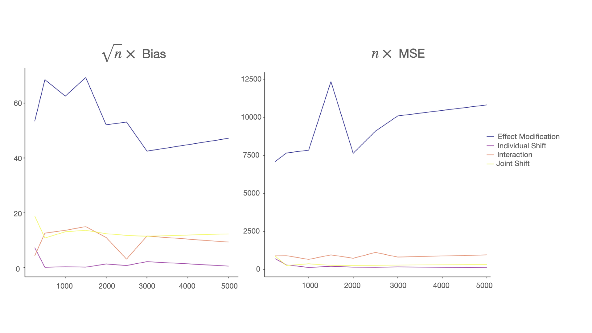
Figure 2: Scaled Bias and MSE

6.4.2 SuperNOVA’s Valid Inference Assessed Through Simulation

To ensure proper inference, we need to demonstrate that SuperNOVA’s estimator has a normal sampling distribution centered at 0 and narrows as the sample size increases. We assess this by examining the empirical distribution of standardized differences. Figure 3 shows the probability density distribution of the standardized bias compared to the true estimates using 50 iterations per sample size. All estimates converge to a mean 0 normal distribution with increasing sample size.

For example, Figure 3 A shows the sampling distribution of the standardized bias for the marginal parameter or an individual shift. We can see that this sampling distribution converges to a normal mean 0 distribution with standard deviation 1. Similarly, Figure 3 B shows the sampling distribution for estimates of a dual shift of two variables to measure the joint impact. Figure 3 C shows estimates for effect modification, which breaks down to estimates of individual exposure shifts within data-adaptively identified regions of a covariate, and Figure 3 D shows the z-score distribution of the interaction parameter estimates. In each case, as sample size increases, the estimates converge to a normal 0, 1 distribution, indicating proper inference for SuperNOVA. Because the effect modification parameter is an average of the counterfactual differences within a covariate region, we still see slight bias at sample size 5000, this is due to averaging over fewer number of observations.

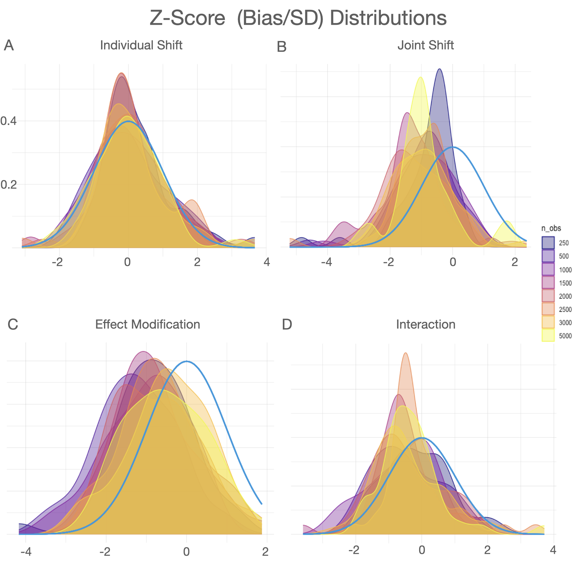
Figure 3: Bias Standardized by Standard Error Compared to Ground-Truth Outcome Under Shift Interventions

7 Applications

7.1 NIEHS Synthetic Mixtures

The NIEHS synthetic mixtures data is a commonly used dataset to evaluate the performance of statistical methods for mixtures. This synthetic data can be considered the results of a prospective cohort study, where the outcome cannot cause the exposures, and correlations between exposure variables can be thought of as caused by common sources or modes of exposure. The nuisance variable Z can be assumed to be a potential confounder and not a collider. The dataset has 7 exposures ($X_{1}-X_{7}$) with a complex dependency structure based on endocrine disruption. Two exposure clusters ($X_{1},X_{2},X_{3}$ and $X_{5},X_{6}$) lead to high correlations within each cluster. $X_{1},X_{2},X_{7}$ positively contribute to the outcome, $X_{4},X_{5}$ have negative contributions, while $X_{3}$ and $X_{6}$ have no impact on the outcome. Rejecting $X_{3}$ and $X_{6}$ is difficult because of their correlations with cluster group members. This correlation and effects structure is biologically plausible, as different congeners of a group of compounds may be highly correlated but have different biological effects. The exposures have various agonistic and antagonistic interactions, and Table 1 provides a breakdown of the variable sets and their relationships. The synthetic data and key for dataset 1 are available on GitHub. Figure 4 shows the marginal dose-response relationships.

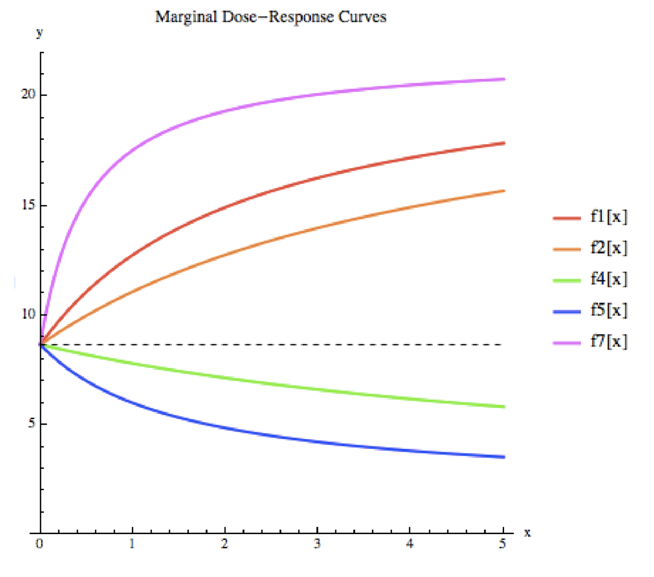
Figure 4: Marginal Dose-Response Relationships

Variables	Interaction Type
X1 and X2	Toxic equivalency factor, a special case of concentration addition (both increase Y)
X1 and X4	Competitive antagonism (similarly for X2 and X4)
X1 and X5	Competitive antagonism (similarly for X2 and X4)
X1 and X7	Supra-additive (“synergy”) (similarly for X2 and X7)
X4 and X5	Toxic equivalency factor, a type of concentration addition (both decrease y)
X4 and X7	Antagonism (unusual kind) (similarly for X5 and X7)

Table 1: NIEHS Synthetic Data Interactions

Given these toxicological interactions we expect these variable sets to be determined in SuperNOVA. For example, we might expect a positive counterfactual result for $X_{1},X_{2},X_{7}$ and negative results for $X_{4},X_{5}$. Likewise, in the case for antagonistic relationships such as $X_{2},X_{4}$, we would expect a joint shift to get closer to the null given $X_{4}$ antagonizes the positive effects of $X_{2}$. For $X_{1},X_{2}$ we would expect the joint shift to be close to the sum of individual shifts (not much interaction) but for $X_{1},X_{7}$ there to be a more than additive effect (some interaction).

The NIEHS data set has 500 observations and 9 variables. Z is a binary confounder. Of course, in this data there is no ground-truth, like in the above simulations, but we can gauge SuperNOVA’s performance by determining if the correct variable sets are used in the interactions and if the correct variables are rejected. Because many machine learning algorithms will fail when fit with one predictor (in our case this happens for g(Z)), we simulate additional covariates that have no effects on the exposures or outcome but prevent these algorithms from breaking.

We apply SuperNOVA to this NIEHS synthetic data using 4-fold CV and the default stacks of estimators used in the Super Learner for all parameters. We parallelize over the cross-validation to test computational run-time on a newer personal machine an analyst might be using. For this set-up, we intentionally use fewer folds (4) which may lead to less consistent findings because less data (75%) is used for the parameter-generating sample to identify the variable relationships compared to say 10 fold where 90% of the data is used.

Condition	Psi	Variance	SE	Lower CI	Upper CI	P-value	Fold	N	Delta
X1	2.00	0.58	0.76	0.51	3.49	0.01	1	125	0.50
X1	5.87	1.08	1.04	3.83	7.91	0.00	2	125	0.50
X1	0.30	1.39	1.18	-2.01	2.61	0.80	3	125	0.50
X1	-0.05	2.56	1.60	-3.18	3.09	0.98	4	125	0.50
X1	1.23	0.28	0.53	0.19	2.27	0.02	Pooled TMLE	500	0.50
X5	-2.12	0.48	0.69	-3.48	-0.76	0.00	1	125	0.50
X5	-1.66	0.75	0.87	-3.36	0.04	0.06	2	125	0.50
X5	-1.20	1.23	1.11	-3.37	0.98	0.28	3	125	0.50
X5	-1.36	0.59	0.77	-2.86	0.14	0.08	4	125	0.50
X5	-1.99	0.24	0.49	-2.94	-1.04	0.00	Pooled TMLE	500	0.50
X7	2.08	0.52	0.72	0.66	3.49	0.00	1	125	0.50
X7	1.98	0.79	0.89	0.24	3.72	0.03	2	125	0.50
X7	2.38	0.97	0.98	0.45	4.31	0.02	3	125	0.50
X7	2.13	0.54	0.73	0.69	3.57	0.00	4	125	0.50
X7	2.11	0.23	0.47	1.18	3.04	0.00	Pooled TMLE	500	0.50
X4	-0.30	0.56	0.75	-1.77	1.18	0.69	1	125	0.50
X4	-0.20	0.79	0.89	-1.94	1.55	0.83	2	125	0.50
X4	0.25	1.15	1.07	-1.86	2.35	0.82	3	125	0.50
X4	-0.29	0.34	0.58	-1.43	0.85	0.62	Pooled TMLE	375	0.50
X2	1.63	0.68	0.83	0.01	3.25	0.05	1	125	0.50
X2	0.00	7.15	2.67	-5.24	5.25	1.00	2	125	0.50
X2	0.15	2.24	1.50	-2.78	3.09	0.92	Pooled TMLE	250	0.50

Table 2: Marginal Results from NIEHS Mixtures Data

Table 2 shows the marginal results from SuperNOVA when applied to this NIEHS synthetic data set using the aforementioned settings. The Condition column shows the variables identified across the folds. Psi shows the counterfactual mean difference under a shift value listed under Delta compared to the observed average outcome. Fold indicates the fold the specific result was found in and N is the number of observations in the fold.

Overall, SuperNOVA accurately rejects exposures $X_{3},X_{6}$, finds marginal effects for $X_{1},X_{5},X_{7}$ consistently in all the folds and effects for $X_{4}$ in three folds and $X_{2}$ in two folds. Directions of the estimates are as expected based on ground-truth where $X_{1},X_{2},X_{7}$ are positive and $X_{4},X_{5}$ are negative. As seen in the dose-response curve, $X_{2},X_{4}$ have the weakest relationships which resulted in fewer fold detections and non-significant findings. The largest effects are for $X_{7}$ which is also true based on the dose-response relationships.

Condition	Psi	Variance	SE	Lower CI	Upper CI	P-value	Fold	N
X5	-1.63	0.76	0.87	-3.34	0.08	0.08	2	125
X7	2.06	0.79	0.89	0.32	3.80	0.03	2	125
X5&X7	0.26	0.91	0.95	-1.61	2.13	0.79	2	125
Interaction	-0.17	0.93	0.96	-2.06	1.72	0.86	2	125
X5	-1.39	0.52	0.72	-2.79	0.02	0.10	4	125
X7	2.16	0.53	0.73	0.73	3.59	0.01	4	125
X5&X7	1.08	0.63	0.80	-0.48	2.64	0.23	4	125
Interaction	0.31	0.49	0.70	-1.07	1.69	0.71	4	125
X5	-1.56	0.35	0.59	-2.72	-0.40	0.04	Pooled TMLE	250
X7	2.20	0.36	0.60	1.02	3.38	0.00	Pooled TMLE	250
X5&X7	0.62	0.42	0.65	-0.65	1.89	0.44	Pooled TMLE	250
Interaction	-0.02	0.38	0.61	-1.23	1.18	0.98	Pooled TMLE	250
X2	-0.21	8.41	2.90	-5.89	5.47	0.90	2	125
X7	2.19	0.79	0.89	0.45	3.93	0.02	2	125
X2&X7	3.44	0.74	0.86	1.76	5.12	0.00	2	125
Interaction	1.46	8.64	2.94	-4.30	7.22	0.39	2	125
X2	1.42	1.00	1.00	-0.54	3.38	0.15	4	125
X7	2.21	0.54	0.73	0.77	3.65	0.01	4	125
X2&X7	2.73	0.63	0.80	1.17	4.29	0.00	4	125
Interaction	-0.90	1.06	1.03	-2.92	1.12	0.37	4	125
X2	0.44	3.12	1.77	-3.02	3.91	0.74	Pooled TMLE	250
X7	2.27	0.36	0.60	1.09	3.46	0.00	Pooled TMLE	250
X2&X7	3.11	0.37	0.61	1.91	4.31	0.00	Pooled TMLE	250
Interaction	0.39	3.21	1.79	-3.12	3.90	0.77	Pooled TMLE	250
X1	5.30	1.22	1.11	3.13	7.47	0.00	2	125
X7	2.01	0.82	0.90	0.24	3.78	0.03	2	125
X1&X7	4.18	0.79	0.89	2.44	5.92	0.00	2	125
Interaction	-3.13	1.29	1.13	-5.35	-0.90	0.00	2	125
X1	5.30	1.22	1.11	3.13	7.47	0.00	Pooled TMLE	125
X7	2.01	0.82	0.90	0.24	3.78	0.03	Pooled TMLE	125
X1&X7	4.18	0.79	0.89	2.44	5.92	0.00	Pooled TMLE	125
Interaction	-3.13	1.29	1.13	-5.35	-0.90	0.00	Pooled TMLE	125
X1	3.56	0.67	0.82	1.95	5.16	0.00	4	125
X5	-1.35	0.51	0.72	-2.76	0.06	0.11	4	125
X1&X5	-0.20	0.52	0.72	-1.61	1.21	0.81	4	125
Interaction	-2.41	0.68	0.82	-4.02	-0.80	0.01	4	125
X1	3.56	0.67	0.82	1.95	5.16	0.00	Pooled TMLE	125
X5	-1.35	0.51	0.72	-2.76	0.06	0.11	Pooled TMLE	125
X1&X5	-0.20	0.52	0.72	-1.61	1.21	0.81	Pooled TMLE	125
Interaction	-2.41	0.68	0.82	-4.02	-0.80	0.01	Pooled TMLE	125

Table 3: Interaction Results from NIEHS Mixtures Data

7.1.1 Comparison to Existing Methods

Currently, quantile g-computation is a popular method for mixture analysis in environmental epidemiology. The method yields estimates of the effect of increasing all exposures by one quantile, simultaneously under linear model assumptions. Quantile g-computation looks like:

$$Y_{i}=\beta_{0}+\sum_{j=1}^{d}\beta_{j}X_{ji}^{q}+\beta Z_{i}+\epsilon_{i}$$

Where $X^{q}$ are the quantized mixture components and $Z$ are the covariates. Which works by first transforming mixture components into quantiles. Then the negative and positive coefficients from a linear model for the mixture components are summed to give a mixture ($\Psi$) summary measure which characterizes the joint impact. There are many assumptions that should be poignant after our discussion of mixtures. Firstly, quantiles may not characterize the exposure-response relationship (could be non-monotonic) which occurs in endocrine disrupting compounds. For interpretable weights and mixture estimate $\Psi$, assumes additive relationship of quantiles ($\Psi$ is just sum of $\beta$’s in front of mixture components). After our discussion, in mixtures our main goal is model possible interactions in the data because we expect exposures to have non-additive, possible non-monotonic, antagonistic and agonistic relationships. Therefore, we should expect interactions in our mixture data. In quantile g-computation, with the inclusion of interactions, the proportional contribution of an exposure to the overall effect then varies according to levels of other variables and therefore weights cannot be estimated. Because we can never assume no interactions, quantile g-computation then boils down to getting conditional expectations when setting mixtures to quantiles through a linear model with interaction terms specified by the analyst. After our discussion of mixtures this should feel incorrect. As we argue, the important variables, relationships, and thresholds in a mixture are all unknown to the analyst which makes this a data-adaptive target parameter problem. Even testing quantile g-computation on the NIEHS data is difficult because we don’t know what interactions to include a priori. The best we can do is run it out of the box and with two-way interactions and compare results to the ground-truth measures. Lastly, quantile g-computation does not flexibly control for covariates.

We run quantile g-computation on the NIEHS data using 4 quantiles with no interactions to investigate results using this model. The scaled effect size (positive direction, sum of positive coefficients) was 6.28 and included $X_{1},X_{2},X_{3},X_{7}$ and the scaled effect size (negative direction, sum of negative coefficients) was -3.68 and included $X_{4},X_{5},X_{6}$. Compared to the NIEHS ground-truth, $X_{3},X_{6}$ are incorrectly included in these estimates. However the positive and negative associations for the other variables are correct.

Next, because we expect interactions to exist in the mixture data, we would like to assess for them but the question is which interaction terms to include? Our best guess is to include interaction terms for all the exposures. We do this and show results in Table 4.

	Estimate	Std. Error	Lower CI	Upper CI	Pr($>$$|$t$|$)
(Intercept)	21.29	1.58	18.19	24.39	0.00
psi1	0.02	1.62	-3.16	3.20	0.99
psi2	0.59	0.67	-0.71	1.90	0.37

Table 4: Quantile G-Computation Interaction Results from NIEHS Synthetic Data

In Table 4 $\Psi_{1}$ is the summary measure for main effects and $\Psi_{2}$ for interactions. As can be seen, when including all interactions neither of the estimates are significant. Of course this is to be expected given the number of parameters in the model and sample size $n=500$. However, moving forward with interaction assessment is difficult, if we were to assess for all 2-way interaction of 7 exposures the number of sets is 21 and with 3-way interactions is 35. We’d have to run this many models and then correct for multiple testing. Hopefully this example shows why mixtures are inherently a data-adaptive problem and why popular methods such as this, although succinct and interpretable, fall short even in a simple synthetic data set.

7.2 NHANES Data

7.2.1 Data Description

The Columbia University Mailman School of Public Health Department of Environmental Health Sciences held a two-day Mixtures Workshop in August 2018 to teach environmental health researchers various statistical methods for studying mixtures. The workshop covered unsupervised methods like clustering, principal component analysis, and exploratory factor analysis, as well as supervised methods like variable selection, weighted quantile sum regression, and Bayesian kernel machine regression. A publicly available real dataset was used to illustrate the methods, taken from a study investigating the association between exposure to persistent organic pollutants and leukocyte telomere length Mitro et al. (2016). The study’s results provided insight into a potential mechanism underlying carcinogenesis mediated by activation of AhR and subsequent telomerase expression, but certain mixtures methods were not utilized resulting in loss of information. The paper by Gibson et al. Gibson et al. (2019) discusses the results obtained using each method on this data during this workshop and how they compare to one another, focusing on understanding how exposure to this mixture may impact LTL.

For our analysis, we used the same population as in the original paper by Mitro et al. Mitro et al. (2016) which investigated the association between exposure to persistent organic pollutants (POPs) with high affinity to the aryl hydrocarbon receptor (AhR) and longer leukocyte telomere length (LTL). The exclusion criteria used in the study are described in Gibson et al. Gibson et al. (2019). This data is from the 2001-2002 National Health and Nutrition Examination Survey (NHANES) cycle, which interviewed 11,039 people, of whom 4,260 provided blood samples and consented to DNA analysis. Sufficient stored samples to estimate telomere length were available for 1,003 participants after excluding individuals without environmental chemical analysis data (n=2,850), those who were missing data on covariates such as body mass index (BMI) (n=70), education (n=2), and serum cotinine (n=8), and those with missing values for individual PCBs, dioxins, or furans (n=327). After filtering for only complete exposures our final study population is nearly identical to the smallest sub-sample included in the original analyses by Mitro et al, our study has 1007 observations compared to 1003 in the original paper.

Exposure assessment was performed as previously described Mitro et al. (2016). Congeners were adjusted for serum lipids which were calculated using an enzymatic summation method. 18 cogeners were used as exposures in our analysis. These breakdown to 8 non-dioxin like PBCs (PCB 74, PCB 99, PCB 138, PCB 153, PCB 170, PCB 180, PCB 187, PCB 194); 2 non-ortho PCBs (PCB 126, PCB 169); 1 mono-ortho PCB (PCB 118); 4 Dioxins (1,2,3,6,7,8-hxcdd, 1,2,3,4,6,7,8-hpcdd, 1,2,3,4,6,7,8,9-ocdd) and 4 Furans (2,3,4,7,8-pncdf, 1,2,3,4,7,8-hxcdf, 1,2,3,6,7,8-hxcdf, 1,2,3,4,6,7,8-hxcd).

Telomere length measurement was performed as previously described Mitro et al. (2016).The quantitative polymerase chain reaction (qPCR) method was used to measure telomere length relative to standard reference DNA (T/S ratio). Samples were assayed three times in duplicate wells, producing six data points which were averaged to calculate mean T/S ratios. Analytical runs were blinded, and the CDC conducted a quality control review. We adjusted for the same covariates as in previous modeling using supervised methods: age, sex, race/ethnicity, educational attainment, BMI, serum cotinine, and blood cell count and distribution. Race/ethnicity was categorized as non-Hispanic white, non-Hispanic black, Mexican American, or other. Educational attainment was categorized as less than high school, high school graduate, some college, or college or more. BMI was categorized as $<25,25-29.9,\geq 30$. Blood cell count and distribution were included as individual covariates: white blood cell count, percent lymphocytes, percent monocytes, percent neutrophils, percent eosinophils, and percent basophils. We include this data as example data in the SuperNOVA package.

We apply SuperNOVA using the default learners in each stack. We use 20-fold CV with no quantile limit for the F-statistic of basis functions. Our default algorithms used in the data-adaptive Super Learner to identify variable relationships include both basis functions and linear terms with up to 2-way interactions. We allow for interactions/effect modification to occur between all 18 POPs and 13 covariates. Given the range of the data, we set a $\delta$ to 2 for all exposures, that is, we investigate the counterfactual differences in telomere length for an increase in 2 ng/g or pg/g for all exposures data-adaptively identified to predict telomere length.

7.2.2 Furan Findings on Telomere Length

Of the 18 POPs we find only one chemical had consistent results across all the folds. No other chemical was used in any of the folds. The furan 2,3,4,7,8-pncdf was identified in all 20 folds. No other marginal effects or interactions were discovered. Table 5 gives a breakdown of the fold specific results and the final pooled TMLE result for an increase in furan 2,3,4,7,8-pncdf by 2 pg/g. The final pooled TMLE estimate shows that a 2 pg/g increase in furan 2,3,4,7,8-pncdf leads to a 0.02 decrease in telomere length.

Condition	Psi	Variance	SE	Lower CI	Upper CI	P-value	Fold	N	Delta
LBXF03LA	0.08	0.00	0.03	0.01	0.14	0.02	1	51	2.00
LBXF03LA	-0.02	0.00	0.03	-0.07	0.04	0.58	2	51	2.00
LBXF03LA	0.02	0.00	0.04	-0.06	0.10	0.66	3	51	2.00
LBXF03LA	0.01	0.00	0.03	-0.04	0.06	0.71	4	51	2.00
LBXF03LA	-0.04	0.00	0.03	-0.09	0.02	0.20	5	51	2.00
LBXF03LA	0.00	0.00	0.03	-0.06	0.07	0.96	6	51	2.00
LBXF03LA	0.03	0.00	0.03	-0.02	0.09	0.24	7	51	2.00
LBXF03LA	0.04	0.00	0.04	-0.03	0.12	0.28	8	50	2.00
LBXF03LA	-0.02	0.00	0.03	-0.08	0.04	0.53	9	50	2.00
LBXF03LA	0.02	0.00	0.02	-0.02	0.06	0.32	10	50	2.00
LBXF03LA	-0.01	0.00	0.03	-0.06	0.04	0.69	11	50	2.00
LBXF03LA	0.07	0.00	0.03	0.01	0.13	0.03	12	50	2.00
LBXF03LA	0.02	0.00	0.02	-0.03	0.07	0.41	13	50	2.00
LBXF03LA	0.01	0.00	0.05	-0.09	0.11	0.81	14	50	2.00
LBXF03LA	-0.01	0.00	0.02	-0.06	0.04	0.66	15	50	2.00
LBXF03LA	0.05	0.00	0.03	-0.00	0.10	0.06	16	50	2.00
LBXF03LA	0.07	0.00	0.03	0.01	0.12	0.01	17	50	2.00
LBXF03LA	0.07	0.00	0.02	0.03	0.11	0.00	18	50	2.00
LBXF03LA	0.02	0.00	0.02	-0.03	0.06	0.49	19	50	2.00
LBXF03LA	0.05	0.00	0.04	-0.03	0.12	0.23	20	50	2.00
LBXF03LA	-0.02	0.00	0.01	-0.03	-0.00	0.04	Pooled TMLE	1007	2.00

Table 5: Furan 2,3,4,7,8-pncdf Lipid Adj (pg/g) Fold Specific and Pooled Findings

The Mitro et al. (2016) summarize results from the workshop. They state that clustering methods identified high, medium, and low POP exposure groups with longer log-LTL observed in the high exposure group. Principal component analysis (PCA) and exploratory factor analysis (EFA) revealed positive associations between overall POP exposure and specific POPs with log-LTL. Penalized regression methods identified three congeners (PCB 126, PCB 118, and furan 2,3,4,7,8-pncdf) as potentially toxic agents. WQS identified six POPs (furans 1,2,3,4,6,7,8-hxcdf, 2,3,4,7,8-pncdf, and 1,2,3,6,7,8-hxcdf, and PCBs 99, 126, 169) as potentially toxic agents with a positive overall effect of the POP mixture. BKMR found a positive linear association with furan 2,3,4,7,8-pncdf, suggestive evidence of linear associations with PCBs 126 and 169, a positive overall effect of the mixture, but no interactions among congeners. These results (in the supervised methods) controlled for the same covariates. Interestingly, although we corroborate the finding of furan 2,3,4,7,8-pncdf, specifically in the BKMR method (the most flexible method used) our results show a negative association. Additionally, we do not find associations of any other POP used in any fold meaning that, in the best fitting spline model, no basis functions for any of the other POPs were used. The inverse association we find compared to these other methods could be a result of our $Q$ model being a Super Learner of many estimators which can model relationships perhaps missed in these other methods.

In this NHANES analysis, we demonstrate that SuperNOVA can effectively identify variable relationships in real-world mixture data and provide estimates for these variables. The resulting summary statistics offer a meaningful estimate of how the outcome would change under an intervention on the identified exposures, providing an interpretable understanding of the results.

8 Software

The development of open-source software for semi-parametric statistical theory is critical for consistent and reproducible results in mixed exposure research. SuperNOVA is an R package that provides an open-source tool for evaluating the causal effects of a mixed exposure using asymptotically linear estimators. This package includes a detailed vignette, documentation of semi-parametric theory, examples of output, and comparison to existing methods. The NIEHS synthetic data and NHANES mixed POP exposure data are also provided for reproducibility. SuperNOVA can run sequentially or in parallel Vaughan and Dancho (2022), and its efficient estimators make it suitable for use on personal machines. The SuperNOVA package is well-maintained, easily accessible, and highly detailed, with coding notebooks that show simulations of mixed exposure data and SuperNOVA output with detailed summaries of interpretation. The package has been made publicly available via GitHub. By making robust statistical software widely accessible, we aim to move beyond simple parametric models and ensure more consistent and accurate results in mixed exposure research.

9 Discussion

In this paper we introduce a new method for estimating the effects of a mixed exposure. Our approach fits a very large statistical model to the exposure-covariate space and treats the basis functions as a data-adaptive target parameter for which we estimate the average change in outcome under stochastic shift interventions. This is done within a cross-validated framework paired with targeted learning of our target parameter which provides estimates that are asymptotically unbiased and have the lowest variance for studies which satisfy the unconfoundedness and positivity assumptions. Our proposed method provides valid confidence intervals without restrictions on the number of exposure, covariates, or the complexity of the data-generating process. Our method first identifies relevant exposure-covariate subspaces that best explains the outcome. The output of our method is the counterfactual mean difference in outcomes if all individual were exposed to a change exposure compared to the observed outcome under observed exposure. Our approach has potentially many important applications including identifying what interacting drugs lead to the most beneficial patient outcomes as well as finding what pollution chemicals interact which leads to deleterious outcomes on public health. Our approach allows for "dredging with dignity" wherein exposure regions can be discovered in the data which are not known a priori and still provide unbiased estimates for the target parameter with valid confidence intervals. The major limitation of our proposed method is the computational burden of density estimation. There are alternative approaches which can be explored. For example, Qin (1998) first propose alternative ways for estimating the probability density ratio needed in our proposed methodology. Instead of relying on estimates of the density estimator $gt$, the problem is recast as a classification problem in an augmented dataset that contains 2n observations. In this dataset, each observation is duplicated, and one is assigned the observed exposure, $At$, and the other is assigned the intervened exposure, $A^{d}_{t}$. An indicator variable, $\Lambda$, is introduced to identify the treatment under intervention. The density ratio can then be expressed as a function of of the probability of $\Lambda$ over 1 - probabilty of $\Lambda$. This approach can be carried out by estimating it via any classification method available in the machine and statistical learning literature, such as Super Learning. This would improve computational time in the case where $\delta$ is not data-adaptive. In the case that it is, this would need to be refit at each iteration and our approach of directly estimating the density may be more efficient as given a density estimator fit new density distributions can be generated via predictions for any $\delta_{i}$. Another limitation to the proposed method is regardind inconsistent findings. In the case that a variable set is identified in every fold interpretation is straightforward; however, in the event that findings are inconsistent interpretation is relative to the analyst. In reporting findings it will become important to also report the number of folds the estimates occur in to give a measure of reliability and consistency in the data. Overall, our simulations with ground-truth, NIEHS synethetic data and real-world data application show the robustness and interpretability of our approach. In an effort to make adoption of semi-parametric methods such as this more seamless we provide the SuperNOVA R package on GitHub which is well documented for analysts to apply to their respective data.

10 Appendix

References

- Meng et al. [2021] Xia Meng, Cong Liu, Renjie Chen, Francesco Sera, Ana Maria Vicedo-Cabrera, Ai Milojevic, Yuming Guo, Shilu Tong, Micheline De Sousa Zanotti Stagliorio Coelho, Paulo Hilario Nascimento Saldiva, Eric Lavigne, Patricia Matus Correa, Nicolas Valdes Ortega, Samuel Osorio, Garcia, Jan Kyselý, Aleš Urban, Hans Orru, Marek Maasikmets, Jouni J.K. Jaakkola, Niilo Ryti, Veronika Huber, Alexandra Schneider, Klea Katsouyanni, Antonis Analitis, Masahiro Hashizume, Yasushi Honda, Chris Fook Sheng Ng, Baltazar Nunes, João Paulo Teixeira, Iulian Horia Holobaca, Simona Fratianni, Ho Kim, Aurelio Tobias, Carmen Íñiguez, Bertil Forsberg, Christofer Åström, Martina S. Ragettli, Yue Liang Leon Guo, Shih Chun Pan, Shanshan Li, Michelle L. Bell, Antonella Zanobetti, Joel Schwartz, Tangchun Wu, Antonio Gasparrini, and Haidong Kan. Short term associations of ambient nitrogen dioxide with daily total, cardiovascular, and respiratory mortality: Multilocation analysis in 398 cities. The BMJ, 372(2), 2021. ISSN 17561833. doi:10.1136/bmj.n534.
- [2]
- Xiao et al. [2021] Lili Xiao, Wei Li, Chunmei Zhu, Shijie Yang, Min Zhou, Bin Wang, Xing Wang, Dongming Wang, Jixuan Ma, Yun Zhou, and Weihong Chen. Cadmium exposure, fasting blood glucose changes, and type 2 diabetes mellitus: A longitudinal prospective study in China. Environmental Research, 192(June 2020):110259, 2021. ISSN 10960953. doi:10.1016/j.envres.2020.110259. URL https://doi.org/10.1016/j.envres.2020.110259.
- Bauer et al. [2020] Julia A. Bauer, Katrina L. Devick, Jennifer F. Bobb, Brent A. Coull, David Bellinger, Chiara Benedetti, Giuseppa Cagna, Chiara Fedrighi, Stefano Guazzetti, Manuela Oppini, Donatella Placidi, Thomas F. Webster, Roberta F. White, Qiong Yang, Silvia Zoni, Robert O. Wright, Donald R. Smith, Roberto G. Lucchini, and Birgit Claus Henn. Associations of a metal mixture measured in multiple biomarkers with IQ: Evidence from italian adolescents living near ferroalloy industry. Environmental Health Perspectives, 128(9):097002–1–097002–12, 2020. ISSN 15529924. doi:10.1289/EHP6803.
- García-Villarino et al. [2022] Miguel García-Villarino, Antonio J. Signes-Pastor, Margaret R. Karagas, Isolina Riaño-Galán, Cristina Rodríguez-Dehli, Joan O. Grimalt, Eva Junqué, Ana Fernández-Somoano, and Adonina Tardón. Exposure to metal mixture and growth indicators at 4–5 years. A study in the INMA-Asturias cohort. Environmental Research, 204, 2022. ISSN 10960953. doi:10.1016/j.envres.2021.112375.
- Zhang et al. [2019] Yuqing Zhang, Tianyu Dong, Weiyue Hu, Xu Wang, Bo Xu, Zhongning Lin, Tim Hofer, Pawel Stefanoff, Ying Chen, Xinru Wang, and Yankai Xia. Association between exposure to a mixture of phenols, pesticides, and phthalates and obesity: Comparison of three statistical models. Environment International, 123(July 2018):325–336, 2019. ISSN 18736750. doi:10.1016/j.envint.2018.11.076.
- Cao et al. [2021] Benfeng Cao, Can Fang, Xiaolin Peng, Xiaoqin Li, Xueting Hu, Pan Xiang, Li Zhou, Hongjie Liu, Yue Huang, Qin Zhang, Shan Lin, Mengke Wang, Yang Liu, Taoping Sun, Sijing Chen, Zhilei Shan, Jiawei Yin, and Liegang Liu. U-shaped association between plasma cobalt levels and type 2 diabetes. Chemosphere, 267(12):1876–1881, 2021. ISSN 18791298. doi:10.1016/j.chemosphere.2020.129224.
- Wang et al. [2020] Bin Wang, Man Cheng, Shijie Yang, Weihong Qiu, Wei Li, Yun Zhou, Xing Wang, Meng Yang, Heng He, Chunmei Zhu, Xingzu Cen, Ailian Chen, Lili Xiao, Min Zhou, Jixuan Ma, Ge Mu, Dongming Wang, Yanjun Guo, Xiaomin Zhang, and Weihong Chen. Exposure to acrylamide and reduced heart rate variability: The mediating role of transforming growth factor-. Journal of Hazardous Materials, 395(March), 2020. ISSN 18733336. doi:10.1016/j.jhazmat.2020.122677.
- Xu et al. [2021] Tao Xu, Bin Wang, Xing Wang, Shijie Yang, Limin Cao, Weihong Qiu, Man Cheng, Wei Liu, Linling Yu, Min Zhou, Dongming Wang, Jixuan Ma, and Weihong Chen. Associations of urinary carbon disulfide metabolite with oxidative stress, plasma glucose and risk of diabetes among urban adults in China. Environmental Pollution, 272:115959, 2021. ISSN 18736424. doi:10.1016/j.envpol.2020.115959. URL https://doi.org/10.1016/j.envpol.2020.115959.
- Billionnet et al. [2011] Cécile Billionnet, Emilie Gay, Séverine Kirchner, Bénédicte Leynaert, and Isabella Annesi-Maesano. Quantitative assessments of indoor air pollution and respiratory health in a population-based sample of French dwellings. Environmental Research, 111(3):425–434, 2011. ISSN 00139351. doi:10.1016/j.envres.2011.02.008.
- Zhou et al. [2016] Yun Zhou, Huizhen Sun, Jungang Xie, Yuanchao Song, Yuewei Liu, Xiji Huang, Ting Zhou, Yi Rong, Tangchun Wu, Jing Yuan, and Weihong Chen. Urinary polycyclic aromatic hydrocarbon metabolites and altered lung function in Wuhan, China. American Journal of Respiratory and Critical Care Medicine, 193(8):835–846, 2016. ISSN 15354970. doi:10.1164/rccm.201412-2279OC.
- Roberts and Martin [2006] Steven Roberts and Michael A. Martin. Using supervised principal components analysis to assess multiple pollutant effects. Environmental Health Perspectives, 114(12):1877–1882, 2006. ISSN 00916765. doi:10.1289/ehp.9226.
- Navas-Acien et al. [2021] Ana Navas-Acien, Arce Domingo-Relloso, Pooja Subedi, Angela L. Riffo-Campos, Rui Xia, Lizbeth Gomez, Karin Haack, Jeff Goldsmith, Barbara V. Howard, Lyle G. Best, Richard Devereux, Ali Tauqeer, Ying Zhang, Amanda M. Fretts, Gernot Pichler, Daniel Levy, Ramachandran S. Vasan, Andrea A. Baccarelli, Miguel Herreros-Martinez, Wan Yee Tang, Jan Bressler, Myriam Fornage, Jason G. Umans, Maria Tellez-Plaza, M. Daniele Fallin, Jinying Zhao, and Shelley A. Cole. Blood DNA Methylation and Incident Coronary Heart Disease: Evidence from the Strong Heart Study. JAMA Cardiology, 6(11):1237–1246, 2021. ISSN 23806591. doi:10.1001/jamacardio.2021.2704.
- Xin Wang, Bhramar Mukherjee and Park [2018] Xin Wang, Bhramar Mukherjee and Sung Kyun Park. Associations of Cumulative Exposure to Heavy Metal Mixtures with Obesity and Its Comorbidities Among U.S. Adults in NHANES 2003-2014. Environment International, 121(Pt 1):683–694, 2018. doi:10.1016/j.envint.2018.09.035.Associations.
- Yitshak-Sade et al. [2020] Maayan Yitshak-Sade, M. Patricia Fabian, Kevin J. Lane, Jaime E. Hart, Joel D. Schwartz, Francine Laden, Peter James, Kelvin C. Fong, Itai Kloog, and Antonella Zanobetti. Estimating the combined effects of natural and built environmental exposures on birthweight among urban residents in massachusetts. International Journal of Environmental Research and Public Health, 17(23):1–16, 2020. ISSN 16604601. doi:10.3390/ijerph17238805.
- McEligot et al. [2020] Archana J. McEligot, Valerie Poynor, Rishabh Sharma, and Anand Panangadan. Logistic lasso regression for dietary intakes and breast cancer. Nutrients, 12(9):1–14, 2020. ISSN 20726643. doi:10.3390/nu12092652.
- Vanderweele [2009] Tyler J. Vanderweele. On the distinction between interaction and effect modification. Epidemiology, 20(6):863–871, 2009. ISSN 10443983. doi:10.1097/EDE.0b013e3181ba333c.
- van der Laan and Rose [2011] M.J. van der Laan and S. Rose. Targeted Learning: Causal Inference for Observational and Experimental Data. Springer Series in Statistics. Springer New York, 2011. ISBN 9781441997821. URL https://books.google.com/books?id=RGnSX5aCAgQC.
- van der Laan and Rose [2018] M.J. van der Laan and S. Rose. Targeted Learning in Data Science: Causal Inference for Complex Longitudinal Studies. Springer Series in Statistics. Springer International Publishing, 2018. ISBN 9783319653044. URL https://books.google.com/books?id=vKFTDwAAQBAJ.
- Glynn and Quinn [2009] Adam N. Glynn and Kevin M. Quinn. An introduction to the augmented inverse propensity weighted estimator. Political Analysis, 18(1):36–56, 2009. ISSN 10471987. doi:10.1093/pan/mpp036.
- Mitro et al. [2016] Susanna D Mitro, Linda S Birnbaum, Belinda L Needham, and Ami R Zota. Cross-sectional associations between exposure to persistent organic pollutants and leukocyte telomere length among us adults in nhanes, 2001–2002. Environmental health perspectives, 124(5):651–658, 2016.
- Künzel et al. [2019] Sören R Künzel, Jasjeet S Sekhon, Peter J Bickel, and Bin Yu. Metalearners for estimating heterogeneous treatment effects using machine learning. Proceedings of the national academy of sciences, 116(10):4156–4165, 2019.
- Wager and Athey [2018] Stefan Wager and Susan Athey. Estimation and inference of heterogeneous treatment effects using random forests. Journal of the American Statistical Association, 113(523):1228–1242, 2018.
- Hubbard et al. [2016] Alan E. Hubbard, Sara Kherad-Pajouh, and Mark J. Van Der Laan. Statistical Inference for Data Adaptive Target Parameters. International Journal of Biostatistics, 12(1):3–19, 2016. ISSN 15574679. doi:10.1515/ijb-2015-0013.
- Zheng and van der Laan [2010] Wenjing Zheng and MJ van der Laan. Asymptotic theory for cross-validated targeted maximum likelihood estimation. U.C. Berkeley Division of Biostatistics Working Paper Series, (273), 2010. URL http://biostats.bepress.com/ucbbiostat/paper273/.
- Nugent and Balzer [2023] Joshua R Nugent and Laura B Balzer. A demonstration of Modified Treatment Policies to evaluate shifts in mobility and COVID-19 case rates in U.S. counties. American Journal of Epidemiology, 01 2023. ISSN 0002-9262. doi:10.1093/aje/kwad005. URL https://doi.org/10.1093/aje/kwad005. kwad005.
- Iván Díaz Muñoz and Mark van der Laan* [2012] Iván Díaz Muñoz and Mark van der Laan*. Population Intervention Causal Effects Based on Stochastic Interventions. Biometrics., 68(2):541–549, 2012. ISSN 15378276. doi:10.1111/j.1541-0420.2011.01685.x.Population. URL https://www.ncbi.nlm.nih.gov/pmc/articles/PMC3624763/pdf/nihms412728.pdf.
- Hejazi et al. [2021] Nima S. Hejazi, Mark J. van der Laan, Holly E. Janes, Peter B. Gilbert, and David C. Benkeser. Efficient nonparametric inference on the effects of stochastic interventions under two-phase sampling, with applications to vaccine efficacy trials. Biometrics, 77(4):1241–1253, 2021. ISSN 15410420. doi:10.1111/biom.13375.
- Hejazi et al. [2022] Nima S Hejazi, Kara E Rudolph, Mark J Van Der Laan, and Iván Díaz. Nonparametric causal mediation analysis for stochastic interventional (in)direct effects. Biostatistics, pages 1–22, 2022. ISSN 1465-4644. doi:10.1093/biostatistics/kxac002.
- Luque-Fernandez et al. [2018] Miguel Angel Luque-Fernandez, Michael Schomaker, Bernard Rachet, and Mireille E. Schnitzer. Targeted maximum likelihood estimation for a binary treatment: A tutorial. Statistics in Medicine, 37(16):2530–2546, 2018. ISSN 10970258. doi:10.1002/sim.7628.
- Smith et al. [2022] Matthew J. Smith, Mohammad A. Mansournia, Camille Maringe, Paul N. Zivich, Stephen R. Cole, Clémence Leyrat, Aurélien Belot, Bernard Rachet, and Miguel A. Luque-Fernandez. Introduction to computational causal inference using reproducible Stata, R, and Python code: A tutorial. Statistics in Medicine, 41(2):407–432, 2022. ISSN 10970258. doi:10.1002/sim.9234.
- Vaart [1998] A. W. van der Vaart. Asymptotic Statistics. Cambridge Series in Statistical and Probabilistic Mathematics. Cambridge University Press, 1998. doi:10.1017/CBO9780511802256.
- Milborrow. Derived from mda:mars by T. Hastie and R. Tibshirani. [2011] S. Milborrow. Derived from mda:mars by T. Hastie and R. Tibshirani. earth: Multivariate Adaptive Regression Splines, 2011. URL http://CRAN.R-project.org/package=earth. R package.
- Ripley and Venables [2021] B. D. Ripley and W. Venables. polspline: Polynomial Spline Routines, 2021. URL https://CRAN.R-project.org/package=polspline. R package version 1.1.26.
- Coyle et al. [2022] Jeremy R Coyle, Nima S Hejazi, Rachael V Phillips, Lars WP van der Laan, and Mark J van der Laan. hal9001: The scalable highly adaptive lasso, 2022. URL https://github.com/tlverse/hal9001. R package version 0.4.3.
- Robins et al. [2013] James M Robins, Peng Zhang, Rajeev Ayyagari, Roger Logan, Eric Tchetgen Tchetgen, Lingling Li, Thomas Lumley, Aad van der Vaart, HEI Health Review Committee, et al. New statistical approaches to semiparametric regression with application to air pollution research. Research report (Health Effects Institute), (175):3–129, 2013.
- Chernozhukov et al. [2018] Victor Chernozhukov, Denis Chetverikov, Mert Demirer, Esther Duflo, Christian Hansen, Whitney Newey, and James Robins. Double/debiased machine learning for treatment and structural parameters, 2018.
- Bickel [1982] Peter J Bickel. On adaptive estimation. The Annals of Statistics, pages 647–671, 1982.
- Schick [1986] Anton Schick. On asymptotically efficient estimation in semiparametric models. The Annals of Statistics, pages 1139–1151, 1986.
- van der Laan Mark et al. [2007] J. van der Laan Mark, Polley Eric C, and Hubbard Alan E. Super learner. Statistical Applications in Genetics and Molecular Biology, 6(1):1–23, 2007. URL https://EconPapers.repec.org/RePEc:bpj:sagmbi:v:6:y:2007:i:1:n:25.
- Marschner [2011] Ian C. Marschner. glm2: Fitting generalized linear models with convergence problems. The R Journal, 3:12–15, 2011.
- Friedman et al. [2010] Jerome Friedman, Trevor Hastie, and Robert Tibshirani. Regularization paths for generalized linear models via coordinate descent. Journal of Statistical Software, 33(1):1–22, 2010. doi:10.18637/jss.v033.i01. URL https://www.jstatsoft.org/v33/i01/.
- Wright and Ziegler [2017] Marvin N. Wright and Andreas Ziegler. ranger: A fast implementation of random forests for high dimensional data in C++ and R. Journal of Statistical Software, 77(1):1–17, 2017. doi:10.18637/jss.v077.i01.
- Chen and Guestrin [2016] Tianqi Chen and Carlos Guestrin. XGBoost: A scalable tree boosting system. In Proceedings of the 22nd ACM SIGKDD International Conference on Knowledge Discovery and Data Mining, KDD ’16, pages 785–794, New York, NY, USA, 2016. ACM. ISBN 978-1-4503-4232-2. doi:10.1145/2939672.2939785. URL http://doi.acm.org/10.1145/2939672.2939785.
- Gibson et al. [2019] Elizabeth A Gibson, Yanelli Nunez, Ahlam Abuawad, Ami R Zota, Stefano Renzetti, Katrina L Devick, Chris Gennings, Jeff Goldsmith, Brent A Coull, and Marianthi-Anna Kioumourtzoglou. An overview of methods to address distinct research questions on environmental mixtures: an application to persistent organic pollutants and leukocyte telomere length. Environmental Health, 18:1–16, 2019.
- Vaughan and Dancho [2022] Davis Vaughan and Matt Dancho. furrr: Apply Mapping Functions in Parallel using Futures, 2022. https://github.com/DavisVaughan/furrr, https://furrr.futureverse.org/.
- Qin [1998] Jing Qin. Inferences for case-control and semiparametric two-sample density ratio models. Biometrika, 85(3):619–630, 1998.