Autonomous search of real-life environments combining dynamical system-based path planning and unsupervised learning

Abstract

In recent years, advancements have been made towards the goal of using chaotic coverage path planners for autonomous search and traversal of spaces with limited environmental cues. However, the state of this field is still in its infancy as there has been little experimental work done. Current experimental work has not developed robust methods to satisfactorily address the immediate set of problems a chaotic coverage path planner needs to overcome in order to scan realistic environments within reasonable coverage times. These immediate problems are as follows: (1) an obstacle avoidance technique which generally maintains the kinematic efficiency of the robot’s motion, (2) a means to spread chaotic trajectories across the environment (especially crucial for large and/or complex-shaped environments) that need to be covered, and (3) a real-time coverage calculation technique that is accurate and independent of cell size. This paper aims to progress the field by proposing algorithms that address all of these problems by providing techniques for obstacle avoidance, chaotic trajectory dispersal, and accurate coverage calculation. The algorithms produce generally smooth chaotic trajectories and provide high scanning coverage of environments. These algorithms were created within the ROS framework and make up a newly developed chaotic path planning application. The performance of this application was comparable to that of a conventional optimal path planner. The performance tests were carried out in environments of various sizes, shapes, and obstacle densities, both in real-life and Gazebo simulations.

Keywords: Autonomous robot, Path planning, Unpredictable search, Nonlinear dynamical system.
Availability of data, material, or code: https://gitlab.com/dsim-lab/paper-codes/Autonomous_search_of_real-life_environments

NOMENCLATURE

$A$	Arnold system’s parameter	$n_{TP_{DS-R}}$	Vector containing the last row of $TP_{DS-R}$
$arnpnt$	Tuple of Arnold system coordinates and accompanied trajectory points	$O_{X,Y}$	Origin of an occupancy-grid map
$B$	Arnold system’s parameter	$PDA$	Occupancy probability data array
$C$	Arnold system’s parameter	$SC_{a}$, $SC_{r_{t}}$	Scan angle and scan range at time $t$
$Cell_{F}$	Representation of a cell with an occupancy probability value of 0	$SR$	Sensing range
$Cell_{O}$	Representation of a cell with an occupancy probability value of 100	$TC_{DS-R}$	Temporary matrix of Arnold dynamical system and robot coordinates
$Cell_{U}$	Representation of a cell with an occupancy probability value of -1	$TF_{MS_{t}}$	Transformation matrix for map frame to sensing frame at a specific time
$Cell_{X,Y}$	Coordinates of a cell in an occupancy-grid map	$Th_{1}$, $Th_{2}$	Cost thresholds
$Cost$	Cost of travel to a trajectory point	$Th_{1}$, $Th_{2}$	Cost thresholds
$c_{z}$	Zone’s coverage rate	$tp$	A potential or current trajectory point for the robot to follow
$CT$	Time for desired coverage rate	$tp_{n-1}$	$tp$ at the last iteration
$DC$	Desired coverage rate	$tp_{new}$	$tp$ used for replacement
$d$	Distance between the robot and a zone centroid	$Tp$	Set of trajectory points
$dist$	Distance between the robot and a cell	$v$	Robot’s velocity
$FOV$	Field of view of the sensor	$x(t),\ y(t),\ z(t)$	Coordinates of the Arnold system
$f,g$	Cost function parameters	$(X,Y)_{M}$, $(X,Y)_{S}$	Point coordinates in the map frame and sensor frame
$H,W$	Height and width of the occupancy grid	$(X,Y)_{RM}$, $(X,Y)_{SM}$	Robot and sensor pose in the map frame, respectively
$ind$	Index number of cell in the probability array	$(X,Y)_{RM_{t}}$, $(X,Y)_{SM_{t}}$	$(X,Y)_{RM}$ and $(X,Y)_{SM}$ at a specific time
$i,j$	Incremental indices	$(X,Y)_{zone}$	Centroid of a zone
$M_{C}$	Matrix storing coverage status and the zone identification of cells	$zid$	Zone identification index
$M_{Z}$	Matrix storing coverage information and the centroid of every zone	$Th_{1}$, $Th_{2}$	Cost thresholds
$n_{iter}$	Number of iterations	$\alpha$	Orientation of a cell from the sensor field of view
$ns$	Set of iterations	$\bar{P}(\text{o})_{Cell_{(X,Y)}}$	Average occupancy probability value representing cost function parameter
${P}(\text{o})_{(X_{i},Y_{i})}$	Occupancy probability value at a coordinate	$\theta$	Mapping variable
$\chi$	Characteristic function

1 Introduction

Coverage path planning (CPP) algorithms are primarily developed for the purpose of creating trajectories that enable a robot to visit an area while avoiding any obstacles. Such algorithms have several applications, from use in varied environments such as households [Choi et al., 2017], farm fields [Hameed, 2014], and surveillance and search tasks [Choi et al., 2020, Di Franco and Buttazzo, 2016, Faigl et al., 2011, Grøtli and Johansen, 2012, Hsu et al., 2014, Kapoutsis et al., 2017, Li et al., 2014, Zhu et al., 2019, Bae, 2004a, Bae et al., 2003]. One of the relatively recent methods of CPP algorithm development is found in the use of chaotic motion, thus the moniker, chaotic coverage path planning (CCPP). Chaotic motion as a basis for coverage path planning opens some potential advantages over other more established CPP algorithms in the area of surveillance missions. It allows the robot to scan uncertain environments while avoiding obstacles as well as adversarial agents, i.e., unpredictability of the motion enables avoiding attacks. Although the generated trajectories appear random to adversaries, the deterministic nature of these planners provide the possibility of being controlled by the designer to adjust the level of unpredictability and quality of coverage.
Studies have used nonlinear dynamical systems (DS) to generate chaotic trajectories [Nakamura and Sekiguchi, 2001, Sridharan et al., 2022, Sridharan and Ahmadabadi, 2020, Volos et al., 2012a, Pimentel-Romero et al., 2017, Nasr et al., 2019, Volos et al., 2013, Tlelo-Cuautle et al., 2014, Volos et al., 2012b, Li et al., 2013, Petavratzis et al., 2021b, Li et al., 2017, Moysis et al., 2021, Petavratzis et al., 2020c, Petavratzis et al., 2021a, Majeed, 2020, Sooraska and Klomkarn, 2010, Bae, 2004b, Bae et al., 2003, Bae, 2004a, Bae et al., 2006, Moysis et al., 2020a, Nwachioma and Pérez-Cruz, 2021, Petavratzis et al., 2020a, Jansri et al., 2004, Zhang, 2018, Chu et al., 2022, Fallahi and Leung, 2010]. Nakamura and Sekiguchi [Nakamura and Sekiguchi, 2001] showed that while algorithms like random walk generate unpredictable trajectories, the density of said trajectories are less uniform than that of chaotic model. This is because the random walk algorithm resists continuity in the robots motion where the chaotic model does not. To build off this earlier work, other studies introduced the chaos manipulation techniques including random number generators [Pimentel-Romero et al., 2017], as well as arccosine and arcsine transformations [Li et al., 2013] to improve dispersal of trajectory points across an environment map. While these methods might have indirectly helped to decrease the coverage time to some extent, they mostly focused on improving the coverage rate rather than the coverage time. Our work in Sridharan et al., 2022 focused on increasing the efficiency of the chaotic path planning approaches by specifically controlling the chaotic trajectories to directly reduce the coverage time. These works proposed various chaos control techniques to make the planner adaptable and scalable to cover environments varying in size and property within a finite time [Sridharan and Ahmadabadi, 2020]. These techniques were successful in significantly reducing the coverage time and bringing it closer to optimal time. While some of these studies have contributed to the subject at hand, the field of CCPP still has much further to go. Most studies discuss techniques which have only been tested in simple environments, such as square shaped simulated environments with little or no variation in obstacle size, shape or density [Sridharan et al., 2022, Li et al., 2013, Petavratzis et al., 2021a, Moysis et al., 2020b, Petavratzis et al., 2020b, Nasr et al., 2019, Pimentel-Romero et al., 2017, Volos et al., 2012a, Volos et al., 2012b, Petavratzis et al., 2021b, Li et al., 2017, Moysis et al., 2021, Petavratzis et al., 2020c, Bae, 2004a, Bae et al., 2003, Bae et al., 2006, Moysis et al., 2020a, Nwachioma and Pérez-Cruz, 2021, Petavratzis et al., 2020a, Jansri et al., 2004, Zhang, 2018, Chu et al., 2022, Fallahi and Leung, 2010]. Additionally, these simulations were not carried out in specialized simulation software like Gazebo and hardly went beyond MATLAB. As a result, the effectiveness of these techniques in real life testing are currently unknown.

The experimental techniques which have been tested in real life have the same limitations in the context of tested environments. Additionally, these experimental techniques do not tackle the challenges in applying CCPP concepts to the real world. For instance, in previous work [Volos et al., 2013, Majeed, 2020, Tlelo-Cuautle et al., 2014, Sooraska and Klomkarn, 2010], the object avoidance strategy deployed is not robust enough to provide continuous chaotic trajectories which maintain kinematic efficiency as the environments become more complex. In the same fashion, there is no dispersal technique to thoroughly spread chaotic trajectories across the environment. The relevance of a dispersal technique becomes especially apparent in larger environments. As for a coverage calculation technique, the maps of the environments were divided into cells of arbitrary size and coverage was based on the number of cells the trajectory passed through. As this method do not use any sensing information, the coverage calculations might become overestimated or underestimated for the following reasons. (1) Without any sensor input, it is difficult to determine if a cell is fully covered or if the robot only covered part of it. (2) The robot can possibly sense multiple cells at once at it moves across the map. Some of these cells may ultimately not be accounted for due to coverage dictated only by trajectory.

The following summarizes the shortcomings of state-of-the-art experimental techniques and the contributions of this paper to address them:

(1) There is no previously defined effective technique for obstacle avoidance which maintains kinematic efficiency and smooth trajectories. This paper proposes a new proactive obstacle avoidance technique that utilizes a cost function and a quadtree [Samet, 1988] data structure created from discretized map data to provide quick chaotic path planning capabilities in complex-shaped environments of varying sizes, shapes and obstacle densities.

(2) There has been no applied means of dispersal of chaotic trajectories in large environments to improve effective coverage, hence reducing coverage time, especially in large and/or complex-shaped environments. This work has developed a map-zoning technique via an unsupervised machine-learning clustering algorithm to disperse chaotic trajectories across the map for more efficient scanning, thus reducing coverage time in large environments.

(3) Lack of accurate and time-effective methods for real-time implementation of coverage calculation in the field of CCPP raises doubt about the applicability of these planners in real-world environments. This study has developed a real-time computation technique that utilizes discretized map data (via quadtree), sensor data, and storage matrices for fast and accurate coverage rate calculation.

To our knowledge, our approach of using quadtree for fast real-time coverage rate computation (with sensor data) is a novel contribution to the field of coverage path planning. Other papers [Huang et al., 2020, Jan et al., 2019] which discussed the use of the quadtree data structure for CPP application, employed it for the purpose of efficient partitioning of the coverage area into smaller regions (and subregions), thus enabling easier identification of the areas in need of coverage.

These contributions were made through the development of algorithms which communicate with each other via the Robot Operating Software(ROS) framework. The rest of the paper is arranged as follows: Section 2 explains the integration of chaotic systems to develop robot trajectory. Section 3 discusses the path planning and chaos control techniques. Section 4 will discuss results of performance in both simulated Gazebo environments and live tests with varying environments, as well as performance comparison with the well-established boustrophedon path planning algorithm. Section 5 concludes the paper and discusses future work. All algorithms developed in this work are written in the Python language.

2 Integration of chaotic dynamical systems for mobile robot

The chaotic dynamical systems can be in form of continuous  [Volos et al., 2012a, Nakamura and Sekiguchi, 2001, Agiza and Yassen, 2001, Li et al., 2016, Lü et al., 2004] or discrete systems  [Li et al., 2013, Arrowsmith et al., 1993, Curiac and Volosencu, 2014, Li et al., 2017, Li et al., 2015]. This work will use the continuous Arnold system simply because our previous study  [Sridharan et al., 2022] showed the potential efficiency and flexibility to adapt and scale to different coverage tasks. The Arnold system  [Nakamura and Sekiguchi, 2001] is described by the following equations:

$$\begin{cases}\mathrm{d}\mathit{x(t)}/\mathrm{dt}=A\sin\mathit{z(t)}+C\cos\mathit{y(t)}\\ \mathrm{d}\mathit{y(t)}/\mathrm{dt}=B\sin\mathit{x(t)}+C\cos\mathit{z(t)}\\ \mathrm{d}\mathit{z(t)}/\mathrm{dt}=C\sin\mathit{y(t)}+B\cos\mathit{x(t)}\ \end{cases}$$ (1)

The variables $x(t)$, $y(t)$, and $z(t)$ are the DS coordinates. $A$, $B$, and $C$ are the Arnold system parameters. A nonlinear dynamical system becomes chaotic upon gaining these properties: (1) sensitivity to initial conditions (ICs), and (2) topological transitivity. Per our previous work  [Sridharan et al., 2022], we use the tuple $(x_{0},y_{0},z_{0})=(0,1,0)$ as initial conditions (ICs) for the Arnold system. The Arnold system parameters are chosen to be $A=0.5$, $B=0.25$, and $C=0.25$. The analysis of the parameter space conducted in our previous study  [Sridharan et al., 2022] showed that these values satisfy the properties (1) and (2) for a chaotic system and result in reasonably uniform coverage of the environment when the Arnold system is integrated into the robot’s controller.

Fig. 1 shows the 3-D chaos attractor of the Arnold system created using these parameters. The CCPP algorithm maps the DS coordinates into the robot’s kinematic equation (Eq. (2)). New states obtained from mapping process are set as trajectory points for the robot to travel to via ROS navigation stack.

$$\begin{cases}\mathrm{d}\mathit{X(t)}/\mathrm{d}t=v\cos\mathit{x(t)}\\ \mathrm{d}\mathit{Y(t)}/\mathrm{d}t=v\sin\mathit{x(t)}\\ \mathit{\omega(t)}=\mathrm{d}\theta(t)/\mathrm{d}t=\mathrm{d}\mathit{x(t)}/\mathrm{d}t\\ \end{cases}$$ (2)

where $X(t)$ and $Y(t)$ are the robot’s coordinates, $v$ is the robot’s velocity, dt is the time step, and $x(t)$ is one of the Arnold system’s coordinates mapped into the robot’s kinematic relations. The other coordinates of the Arnold system can replace $x(t)$ to perform the mapping, however, the trajectories produced by each coordinate will be different from the others. We will later use this feature in section 3.1.1 to improve coverage. Fig. 2 illustrates the general schematics of a two wheel differential drive mobile robot used in this study. The robot comprises of two active fixed wheels with one passive caster, subject to a non-holonomic constraint.

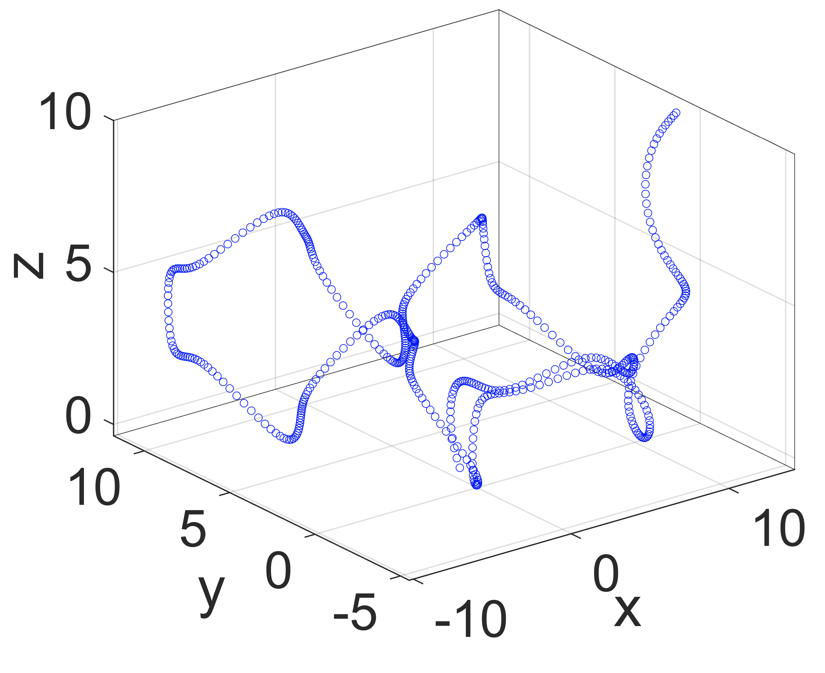
Figure 1: 3-D Chaos attractor for the Arnold system, first published in [Sridharan et al., 2022] by Springer Nature.

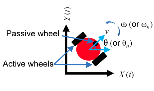
Figure 2: Mobile robot’s motion on a plane, first published in [Sridharan and Ahmadabadi, 2020] by IEEE.

3 Path planning strategy and chaos control technique

The objective of this work is to tackle the challenges associated with experimental real-time implementation of CCPP. We adapt some of the theoretical chaos control techniques proposed in our previous study [Sridharan et al., 2022] and make them applicable to real-life environments while providing the following contributions. (1) A proactive obstacle avoidance technique which utilizes a cost function and a quadtree data structure created from discretized map data to set trajectories away from obstacles while maintaining general smoothness of trajectory and continuous motion. (2) A map-zoning technique based on an unsupervised machine-learning clustering algorithm which continuously directs the robot to less-visited distant areas of the environment. And (3) a computation technique which is independent of cell size, but instead based on discretized map data (via quadtree) and sensor data to provide accurate real-time coverage calculation.

$$ind=(Cell_{X}\times W)+Cell_{Y}$$ (3)

$$\begin{cases}X_{M}=(Cell_{X}\times res)+O_{X}\\ Y_{M}=(Cell_{Y}\times res)+O_{Y}\end{cases}$$ (4)

$$\begin{cases}Cell_{X}=ind\bmod W\\ Cell_{Y}=\frac{(ind-Cell_{X})}{W}\end{cases}$$ (5)

$$\begin{cases}Cell_{X}=\frac{X_{M}-O_{X}}{res}\\ Cell_{Y}=\frac{Y_{M}-O_{Y}}{res}\end{cases}$$ (6)

In what follows: (1) the algorithms interact with map data information of a 2D occupancy-grid map. (2) Cells refer to the smallest possible segments of the map, while zones represent larger segments. (3) The relevant map data information includes: occupancy probability data array ($PDA$), map resolution ($res$), map height ($H$), map width ($W$), and origin of map ($O_{(X,Y)}$). (4) The $PDA$ contains the occupancy probability values of every cell in the occupancy-grid map and the algorithms interact with this information in various ways. Eqs. (3)-(6) are used in several algorithms to convert relevant data field information to useful formats to perform various tasks. Eq. (5) derives the coordinate of a cell in the occupancy-grid map ($Cell_{(X,Y)}$) from its corresponding $PDA$ index value ($ind$). Eq. (6) derives the coordinates of a cell ($Cell_{(X,Y)}$) using the $O_{(X,Y)}$ and its map frame coordinate ($(X,Y)_{M}$). (5) The map of the environment is broken into individual zones before all other algorithms start to run. (6) The quadtree data structure solely contains the $Cell_{(X,Y)}$ positions of every cell which represents free space. The quadtree and the storage matrices ($M_{Z}$ and $M_{C}$) are created (directly or indirectly) using relevant map data information (before the start of any algorithms excluding the unsupervised machine-learning clustering algorithm) for quick queries and zone coverage updates. The quadtree algorithms developed in [Quadtree implementation in Python, 2020] have been adapted for this work. (7) The transformation matrix ($TF_{MS}$) (created via ROS) transforms point coordinates from the map frame to the sensor frame and is used along with sensor data for coverage calculation. (8) The communications between any algorithms that do not directly invoke each other is performed via the ROS framework. (9) As the robot moves across the map, trajectory points are set as goals by the ROS navigation stack. The navigation stack provides a global path planner based on the Dijkstra algorithm. The DWA and TEB Local planners were tested to see which would be the best. In the final analysis, a DWA local planner is chosen with full awareness of the sub-optimal trajectories it often generates. However, the DWA local planner was chosen for the following reasons: (i) it is less sensitive to the choice of parameters, making it easier to tune and use in different environments. (ii) It can handle real-world scenarios of dynamic obstacles more effectively, as it takes into account the motion of the robot and the motion of other objects in the environment when planning a path. And (iii) it is computationally less expensive, making it more suitable for use on robots with limited computational resources. (8) It must be noted that all algorithms are written in the Python language and therefore any indices of any vectors, arrays or matrices discussed starts at 0.

The rest of this section will provide an overview of the CCPP process in ROS using the flowchart shown in Fig. 3. As seen, the first step is to create the occupancy-grid map via simultaneous localization and mapping (SLAM). The resulting occupancy grid map is then published as map data. As discussed earlier, part of the map data is the $PDA$. The $(X,Y)_{M}$ values of all cells that represent free space, are derived from the $ind$ values of the aforementioned cells in the $PDA$ (using Eqs. (5) and then (4)). These $(X,Y)_{M}$ values are stored in an array which is fed as part of the input to the clustering algorithm. The clustering algorithm uses this information to divide the environment into zones. The matrix $M_{Z}$ stores zones information. The storage matrix $M_{C}$ is created using all the index information from the $PDA$ and zones information. $M_{C}$ keeps track of cell coverage to memory. Then, the chaotic coverage path planning procedure is carried out as thus: The ArnoldTrajectoryPlanner ($ATP$) function, as outlined in Algorithm 1, employs the Arnold system to continuously generate chaotic trajectories within the map frame until the desired coverage ($dc$) is achieved. Algorithm 1 utilizes the information provided by the $PDA$ to facilitate obstacle avoidance decision-making. In response to the information provided by the $PDA$, Algorithm 1 interacts with Algorithms 2 and 3, directing chaotic trajectories away from obstacles. Algorithm 2 (called by Algorithm 1) leverages the quadtree and a two-parameter cost function. Algorithms 2 and 3 exchange information to calculate these two parameters, which they subsequently relay to Algorithm 1. Meanwhile, Algorithm 5 plays a role in publishing data regarding the least-covered zones. Algorithm 1 utilizes this information to strategically distribute chaotic trajectories across the map. Algorithm 4 receives published data from the ROS sensor_msgs and ROS tf package, which it combines with information from the quadtree to calculate total coverage ($tc$) with the help of Algorithm 5. Algorithm 5 updates the information in the storage matrices $M_{C}$ and $M_{Z}$ to keep track of the coverage of every zone. $M_{C}$ keeps track of covered cells and $M_{Z}$ tracks zone coverage. Algorithm 4 then uses the information in $M_{Z}$ to calculate $tc$. Each iteration of Algorithm 4 uses up-to-date sensor data and $TF_{MS}$ to accurately calculate $tc$ until $dc$ is reached. Once $dc$ is reached, Algorithms 4 and 1 are prompted to stop. The initial position of the robot in the map frame ($(X,Y)_{RM}$) is used as a starting point to generate trajectory points successively. $(X,Y)_{RM}$ is retrieved from the transformation of odometry data using the tf package. Next section starts with discussing the obstacle avoidance technique and explains the interaction between the Algorithms 1, 2, and 3.

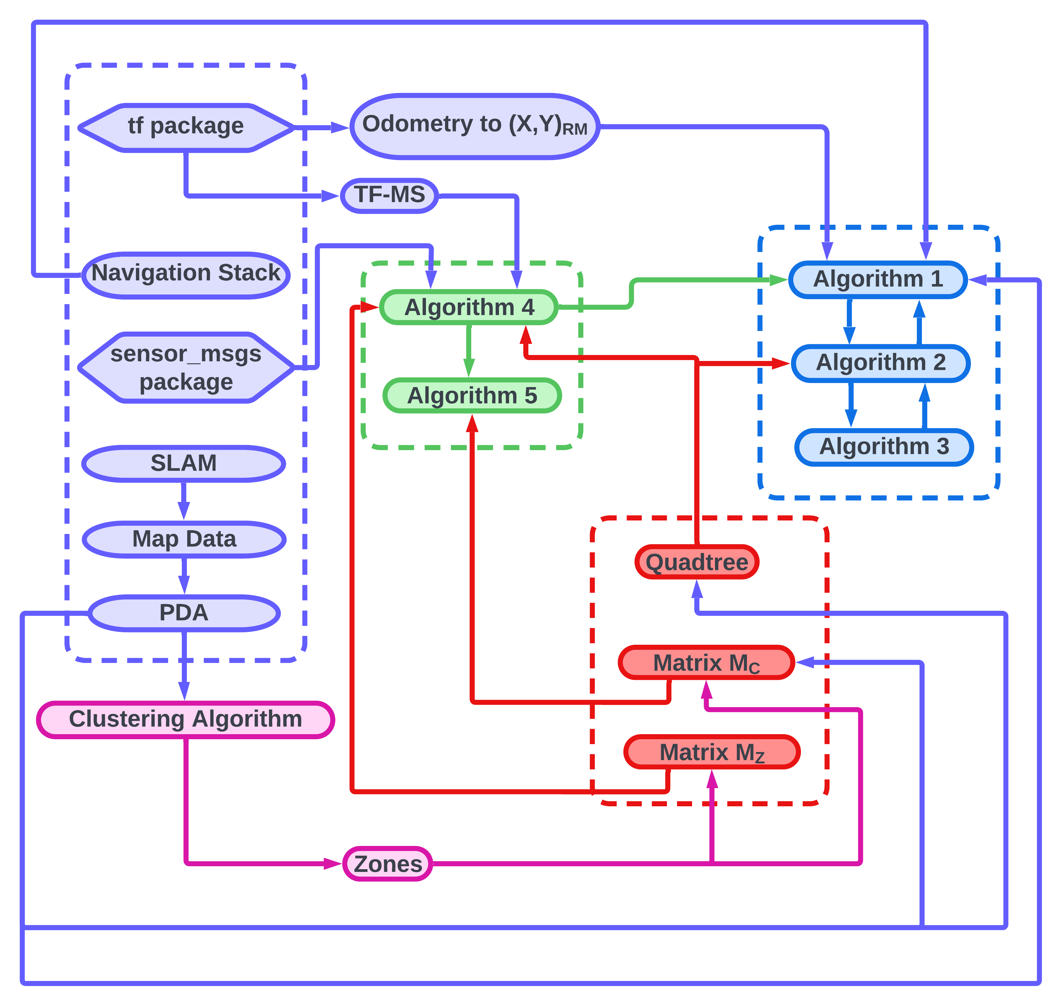
Figure 3: Flowchart showing algorithm flow in the ROS1 environment.

3.1 Obstacle avoidance Techniques

The proposed obstacle avoidance technique uses a quadtree and cost function to generate smooth and continuous trajectories around obstacles and provide quick chaotic path planning capabilities in environments varying in size, shape, and obstacle density. Our work creates this quadtree from descritized map data to quickly access occupancy-grid map coordinates representing free space. Conceptually, our technique works as follows: (1) The corresponding $PDA$ index value ($ind$) of the trajectory point ($tp$) is calculated and evaluated in the $PDA$ to check its probability value. Probability values $\neq$ 0 are deemed non-viable. (2) Cells representing free space within some radius ($r$) of a non-viable $tp$ are accessed from the quadtree (via querying [Quadtree implementation in Python, 2020]). It should be noted that the $r$ value is chosen based on the $res$ of the occupancy-grid map. The $res$ for all simulations and tests is 0.05 meters per pixel. The tested maximum $r$ value of 19 cell lengths value does not reduce computation speed. (3) Each coordinate is evaluated using a cost function to determine a favorable replacement coordinate. (4) A replacement coordinate is set as the new $tp$. In scenarios where there are no free cells in the immediate vicinity of a non-viable $tp$ for replacement, additional processes are carried out to generate a viable $tp$. This case, as well as other special scenarios, will be further discussed in section 3.1.1. Quick access to cell information is critical for fast computation, allowing these steps to take place within a sufficiently short time frame, which is essential for achieving obstacle avoidance without the need to stop motion. General smoothness of the trajectory is maintained as the ROS navigation stack sets the robot to these favorable coordinates. It should be noted that the ROS navigation stack sets the next successive goal once the robot is within some threshold of the current one. This threshold is set to a certain length based on the ROS path messages [nav_msgs/Path.msg, 2023], which provide a list of coordinate points that the robot follows on the path to a goal. In this way, the robot’s continuous motion is not hindered.

Algorithm 1 *

Algorithm 1 (main): $ArnoldTrajectoryPlanner(A,B,C,v)$

1:  $|TP_{DS-R}|_{first\ row}\leftarrow$ [$x_{0},y_{0},z_{0}$,$(X,Y)_{RM}$]

2:  while $tc\ <\ dc$ do

3:     if $\sum_{i=1}^{n}ns==n_{iter}$ OR successive bad runs then

4:        $(X,Y)_{\text{zone}}\leftarrow$ $\min\limits_{zid_{1},\dots zid_{T}}\leftarrow CoverageCalculator()$

5:        $(Cost,tp_{new})\leftarrow Shift((X,Y)_{zone},tp_{n-1},0)$

6:        robot navigates to $tp_{new}$

7:        $TP_{DS-R}\leftarrow$ [$x_{0},y_{0},z_{0},tp_{new}$]

8:     end if

9:     if $\sum_{i=1}^{n}ns<n_{iter}$ then

10:        if set $ns$ ends with the generation of a viable $tp$ then

11:           $TP_{DS-R}\leftarrow n_{TP_{DS-R}}$

12:        end if

13:        if the generation of previous set $ns$ is interrupted by a $tp$ set outside boundaries then

14:           $(Cost,tp_{new})\leftarrow Shift((X,Y)_{RM},tp_{n-1},0)$

15:           $TP_{DS-R}\leftarrow$[$x_{0},y_{0},z_{0},tp_{new}$]

16:        end if

17:     end if

18:     $Tp=[\ ]$

19:     $n_{TP_{DS-R}}\leftarrow TP_{DS-R}$

20:     sub algorithm 1 – First stage

21:     sub algorithm 2 – Second stage

22:  end while

3.1.1 Algorithm workflow

Algorithm 1 uses the Runge-Kutta fourth-order (RK4) method to propagate Eqs. (1) and (2), and therefore calculates the approximate states of the Arnold system as time progress. As the evolution of one of the Arnold system DS coordinates ($DS_{index}$) is mapped onto the robot’s kinematics, a chaotic trajectory is created. It is important to note that the robot does not initially try to move to every trajectory point ($tp$) as it is created. This means that Algorithm 1 goes through a set of several iterations ($ns$) at a time, to create a set of trajectory points ($Tp$) which describe a chaotic trajectory. Algorithm 1 might then retroactively modify the trajectory points that describe the chaotic trajectory when the robot tries to successively move to each $tp\in$$Tp$. The algorithm was developed this way as this promoted generally smoother trajectories as well as a better local spread of trajectories within the robot’s local area around areas of high obstacle density. Therefore $ns$ ¿ 1 as opposed to $ns$ = 1. In summary, the robot has a general continual chaotic path to follow within its local area, and changes can be made to that path for object avoidance. This is the reason that a large bulk of Algorithm 1 is developed into two stages. Each stage is a for-loop. The first stage is described in sub-algorithm 1, and the second stage is described in sub-algorithm 2. In the first stage, trajectory points are successively generated via RK4 method to make up the set $Tp$. At this stage, a trajectory point ($tp$) might be replaced (for obstacle avoidance) before it is added to the set. Therefore every trajectory point ($tp$) $\in Tp$ affects the next $tp$ as each $tp$ was successively calculated from the last. Set $Tp$ establishes some chaotic path. In the second stage, the robot tries to follow this chaotic path. Replacement of any $tp\in Tp$ at this stage does not affect the next $tp$ as the general chaotic path was already established in the first stage. In this way there is higher likeliness of continuity of chaotic trajectory due to how the process creates replacement trajectory points at each stage. This becomes clear in the next paragraphs which provide full explanations of the sub-algorithms processes.

In what follows, cells representing free space, obstacle space, and unknown space are designated as $Cell_{F}$, $Cell_{O}$, and $Cell_{U}$, respectively. In Algorithm 1, the RK4 method approximates the state of the Arnold System every time step ($\Delta t$) of 2.75 seconds. This time step ensures the generation of sufficiently smooth trajectories. It is important to note that unknown space represents areas within the map where the state of occupancy is not yet determined. These areas are usually represented by cells in the occupancy-grid map that have not been sensed by the sensor during SLAM. These cells are usually surrounded by cells representing obstacle space. Each stage of Algorithm 1 will make use of a custom cost function which sets trajectories away from obstacles. The first stage makes use of a threshold ($Th_{1}$) to judge the cost of any replacement $tp$ to improve the odds involved in the search for highly favorable replacement coordinates. The second stage makes use of threshold ($Th_{2}$) which is of a smaller value than $Th_{1}$. This threshold is used as a contingency to check for any viable $tp$ set too close to an obstacle. In this way, said $tp$ can be immediately replaced before it is set as a goal (via ROS) in stage 2. Following this overview of the two stages, the sub-algorithms are explained in the next paragraphs.

Algorithm 2 *

Algorithm 1 (sub-algorithm 1): $ArnoldTrajectoryPlanner(A,B,C,v)$

1:  for $i<ns$ do

2:     $arnpnt\leftarrow$ Eqs. (1) and (2) with $n_{TP_{DS-R}},A,B,C,v,dt$ and $DS_{index}$

3:     $tp\leftarrow arnpnt$

4:     if $tp$ is set at a coordinate which does not exist within the occupancy-grid map boundaries then

5:        drop this $tp$

6:        Break

7:     end if

8:     if $tp$ is viable then

9:        $Tp,n_{TP_{DS-R}},TP_{DS-R}\leftarrow$ store and update relevant information to memory

10:     end if

11:     if $tp$ is not viable then

12:        $(Cost,tp_{new})\leftarrow Shift(tp,tp_{n-1},1)$

13:        if $Cost\geq Th_{1}$ then

14:           $arnpnt\leftarrow$ Eqs. (1) and (2) with $n_{TP_{DS-R}},A,B,C,v,dt$ and a different $DS_{index}$

15:           If creation of viable $tp$ is unsuccessful OR $Cost\geq Th_{1}$(after use of $Shift$ function), continue $DS_{index}$ switching.

16:           Upon exhaustion of $DS_{index}$ switching choose the $tp_{new}$ associated with the lowest $Cost$. The RK4 approximation ($arnpnt$) of said $tp$ is stored to memory.

17:        end if

18:     end if

19:  end for

In an iteration of the first stage (sub-algorithm 1),the RK4 method generates a $tp$ with its accompanied $DS$ coordinates. As a reminder, the $tp$ and $DS$ coordinates represent the kinematic and Arnold system states respectively. Both the $DS$ coordinates and associated $tp$ are paired together and denoted as $arnpnt$. If $tp$ is viable, it is added to set $Tp$. Any $tp$ generated outside the boundaries of the occupancy-grid map are added to set $Tp$. Upon addition, the for loop breaks immediately. A non-viable $tp$ goes through a procedure which tries to find a suitable replacement $tp$ ($tp_{new}$) by utilizing Algorithm 2. It is important to note that in the scenario where there is no single $Cell_{F}$ to be queried within $r$ cell lengths of a non-viable $tp$, this $tp$ is assigned as a $tp_{new}$ of the highest possible cost ($Cost_{max}$). This is represented in lines 3-4 of Algorithm 2. This cost value is greater than any possible cost which could be assigned. If the $Cost$ of the $tp_{new}$ found via Algorithm 2 is $\geq Th_{1}$, this stage utilizes deterministic $DS_{index}$ switching to generate new $tp$ (via RK4 method). That is, a different $DS$ coordinate representing the current Arnold system state is mapped onto the robot’s kinematics. This $tp$ goes through the same process as the $tp$ created from the previous mapping. If $DS_{index}$ switching is exhausted, the $tp_{new}$ associated with the least cost is chosen along with the accompanied DS coordinates (to make $arnpnt$) for the next iteration. In the event that this process still results in the selection of an unreplaceable non-viable $tp$, the algorithm proceeds with this $tp$. It is added to set $Tp$ and will be replaced at stage 2. It must be noted that the next iteration uses the original $DS$ coordinate before $DS_{index}$ occurred. Algorithm 1 attempts to replace non-viable $tp$ at stage 1 rather than shutting down the $tp$ generation process (via breaking the loop) for the following reasons. Replacing $tp$ induces a higher likelihood of spreading the chaotic trajectory across the local area around the robot’s position, thus increasing the likelihood of covering new cells at a faster rate (ultimately reducing $CT$). In other words, breaking the loop at any unreplaceable non-viable $tp$ might cause a situation where very few $tp$ are being generated in the robot’s local area leading to inefficient coverage. This whole process also induces likeliness of continuity and smoother trajectories because: (1) an unreplaceable $tp$ may still generate a viable $tp$ in the next iteration (2) trajectory points generated from different $DS$ coordinates of the same Arnold system state are not too dissimilar from each other to cause the overall chaotic trajectory (described by set $Tp$) to lose continuity.

Algorithm 3 *

Algorithm 1 (sub-algorithm 2): $ArnoldTrajectoryPlanner(A,B,C,v)$

1:  for $tp\in Tp$ do

2:     if $Cost\geq Th_{2}$ OR non-viable $tp$ then

3:        $(Cost,tp_{new})\leftarrow Shift((X,Y)_{RM},0)$

4:     end if

5:     robot navigates to $tp$

6:  end for

The second stage (sub-algorithm 2) provides an additional measurement to replace any $tp\in Tp$ $\geq Th_{2}$, as well as any non-viable $tp\in Tp$ that could not be replaced in the first stage. This stage successively scrutinizes each $tp\in Tp$ within Algorithm 2 immediately before setting it as a goal. During replacement, Algorithm 2 chooses a favorable coordinate by scrutinizing all $Cell_{F}$ within $r$ of robot’s current position ($(X,Y)_{RM}$). Any $tp$, with cost greater than $Th_{2}$, goes through the same process as a non-viable $tp$. The replacement $tp$ is paired with the $DS$ coordinates of the $tp$ that was replaced.

In order to establish a continuation between the successive sets of $ns$, the last pair of $DS$ coordinates and $tp$ ($n_{TP_{DS-R}}$) generated in the last iteration becomes the IC for the next set of iterations. However, if the generation of the previous iterative set $ns$ was interrupted by an iteration in which $tp$ was set outside the boundaries, Algorithm 1 calls Algorithm 2 to find a favorable point coordinate around the $(X,Y)_{RM}$ as part of new IC. This therefore completely breaks the continuation of the current chaotic evolution for a new evolution. After some total number of iterations ($n_{iter}$), Algorithm 1 makes a decision to have the robot move to the center of the least covered zone, at which point a new chaotic evolution starts with the pair of ($x_{0},y_{0},z_{0}$) and some $(X,Y)_{M}$ at the center of the least covered zone as IC. The same process occurs when the creation of successive sets of $ns$ were interrupted, resulting in the creation of only a few viable $tp$. Algorithm 4 ($CoverageCalculator$) communicates information identifying the least covered zone. It must be noted that not chaotic path is generated from the robot’s current position to the least covered zone. This is important as $(X,Y)_{RM}$ might be far away from the least covered zone, and the ROS navigation stack may generate a very predictable path towards the least covered zone. Section 3.1.2 discusses the cost function in detail.

Algorithm 4 *

Algorithm 2: $Shift(tp,tp_{n-1},\lambda)$

1:  Query every $Cell_{F}$ within $r$ of $tp$

2:  if Query = 0 then

3:     $tp_{new}$ = $tp$; the non-viable $tp$ could not be replaced

4:     return  $|Cost_{max},tp_{new}|$

5:  else

6:     $(Cost,tp_{new})\leftarrow argmin_{Cell_{F}\in Query}\ CostCalculator(Cell_{F})\ +\ \lambda\|tp-tp_{n-1}\|_{2}$

7:     return  $(Cost,tp_{new})$

8:  end if

Algorithm 5 *

Algorithm 3: $CostCalculator(Cell_{(X,Y)})$

1:  $\bar{P}(\text{o})_{Cell_{(X,Y)}}=\frac{1}{n}\sum_{i=1}^{n}P(\text{o})_{(X_{i},Y_{i})}\cdot\chi(\sqrt{(X_{i}-X_{Cell_{(X,Y)}})^{2}+(Y_{i}-Y_{Cell_{(X,Y)}})^{2}}\leq l)$

2:  return  $g\leftarrow\bar{P}(\text{o})_{Cell_{(X,Y)}}$

3.1.2 Custom cost functions

Algorithms 2 and 3 use a cost function (Eq. (7)) to help Algorithm 1 generate trajectory points away from obstacles. Algorithms 2 and 3 calculate cost function parameters $f$ and $g$, respectively. In Eq. (7), the parameter $f$ is the distance between the generated $tp$ in the last iteration ($tp_{n-1}$) and the point coordinate ($(X,Y)_{M}$) of the $Cell_{F}$ being evaluated. The $Shift$ function (Algorithm 2) calculates $f$. The variable $g$ expresses the closeness of a $Cell_{F}$ to obstacle and/or unknown space. The parameter $g$ is the average of assigned values of the coordinates within range $l$ (6 cell lengths) of the $Cell_{F}$ being evaluated. The assigned values are as follows: (1) Any coordinate position which matches a cell position is assigned the absolute value of the occupancy probability of that cell. The probability values of $Cell_{O}$, $Cell_{U}$ and $Cell_{F}$ are 100, -1, and 0 respectively. (2) Any coordinate position which does not match a cell location, in other words, is not within the occupancy-grid boundaries is assigned a value of 500. Such a position is assigned the highest cost so as to set trajectories away from the occupancy-grid map boundaries. Additionally, this will reduce the likelihood of generating trajectory points outside the boundaries. The $tp_{new}$ is derived from the cell associated with the lowest $Cost$. The $\lambda$ input is set to 0 when using $(X,Y)_{RM}$ as seed for query so as to set $f$ to 0. In Algorithm 3, $\chi$ is a characteristic function which evaluates to 1 if the $(X,Y)_{i}$ coordinate is within range $l$ of the position of the evaluated $Cell_{F}$.

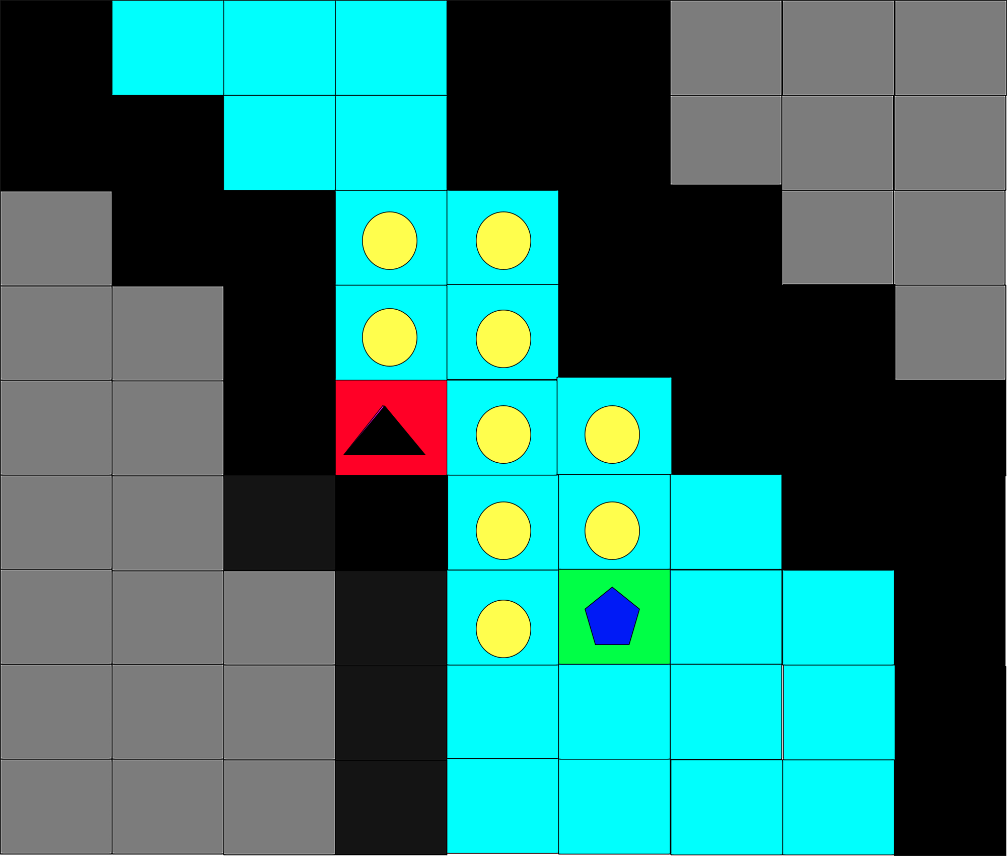
Figure 4: Process for replacement of a non-viable $tp$ for $r=2$ and $l=1$. Triangle: non-viable $tp$; Circle: $Cell_{F}\in Query$; and Pentagon: $tp_{new}$.

Fig. 4 shows an example of this process. Algorithm 2 successively evaluates each $Cell_{F}\in Query$ (cells with circles and pentagon markers), all within $r$ cell lengths of non-viable $tp$ (red cell with triangle marker) with the aid of Algorithm 3 and selects the one with the lowest cost (cell with pentagon marker). This is the only $Cell_{F}\in Query$ completely surrounded by other $Cell_{F}$ within $l$ cell lengths of itself. If multiple $Cell_{F}\in Query$ share the lowest cost value calculated, the first $Cell_{F}\in Query$ to be evaluated at that cost value is chosen for $tp_{new}$.

$$Cost=f+g$$ (7)

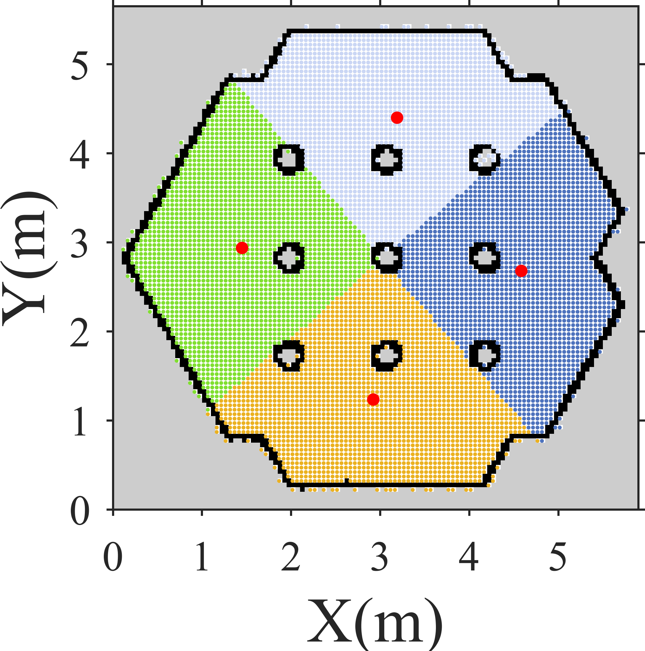
(a)

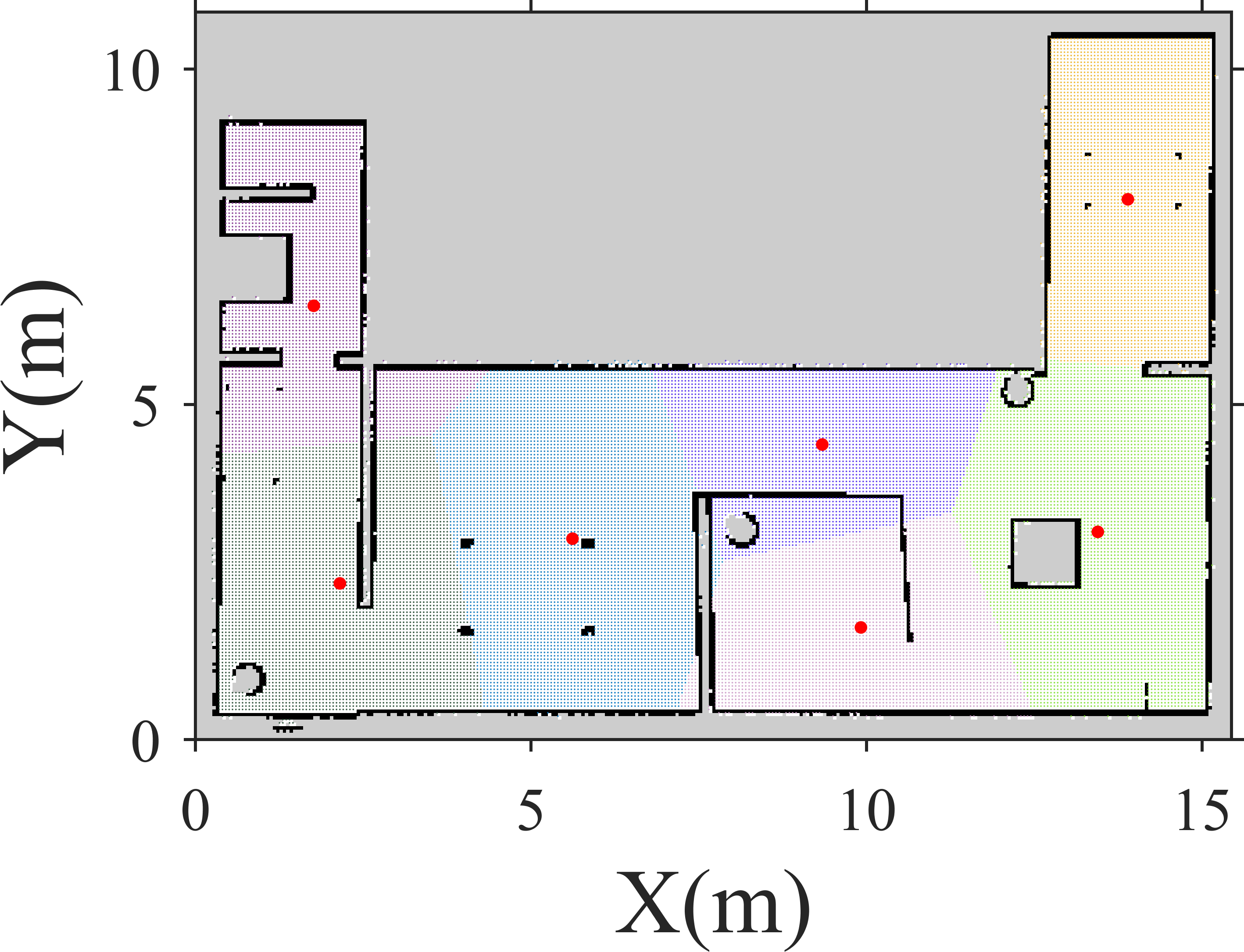
(b)

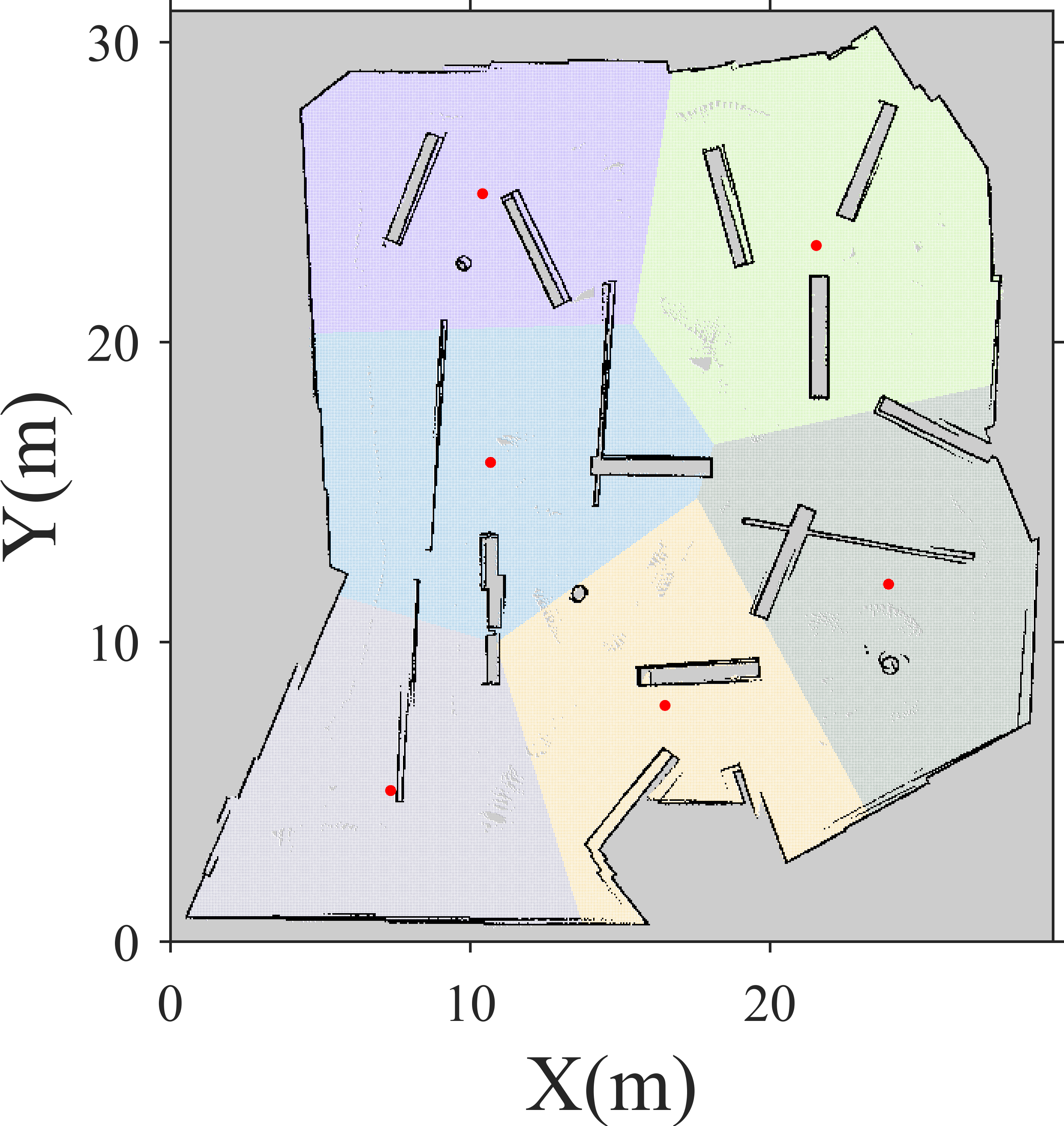
(c)

Figure 5: Map-zoning technique showcased on maps of environments of various sizes shapes and obstacle configurations. Filled circle: centroid of each zone; same-colored small dots: a specific zone.

3.2 Map-zoning Technique

This technique uses an unsupervised machine-learning clustering algorithm to break the map into individual zones, dispersing chaotic trajectories across the map for more effective scanning and reducing coverage time in large and/or complex environments. The clustering process takes place before the start of the coverage; it groups the $(X,Y)_{M}$ coordinates of all $Cell_{F}$ into different zones. The clustering algorithms were obtained from the scikit-learn Python library. Several tests led to the selection of two agglomerative clustering algorithms, ward and k-means, which worked best for grouping cells in a sensible manner. K-means was ultimately chosen because it could create clusters for larger maps, while the ward algorithm ran into memory errors for those maps. The parameters of the k-means algorithm were set to enable sensible centroid assignment and cluster formation (see Figs. 5(a)-(c)) within a reasonable computation time. The centroid of a cluster represents the midpoint ($(X,Y)_{zone}$) of the zone. Each zone’s midpoint and coverage are stored in memory so that the coverage is continuously updated as the robot traverses the map, and the $(X,Y)_{zone}$ of the least covered zone can be published by Algorithm 4. If there are multiple zones with the least coverage, the $(X,Y)_{zone}$ of the closest distance $d$ to the robot’s current position is published. Matrix $M_{Z}$ stores information about the individual zones, with columns containing the following data from left to right: $X_{zone}$, $Y_{zone}$, the number of $Cell_{F}$ in each zone, the number of $Cell_{F}$ covered in a zone, and the zone’s coverage rate ($c_{z}$).

Algorithm 4 utilizes $M_{Z}$ to analyze which zones are least covered. The coverage of every zone is updated by the $Worker$ function (Algorithm 5), which is invoked by Algorithm 4. Algorithm 1 receives $(X,Y)_{zone}$ messages to spread the chaotic trajectories. To do so, Algorithm 1 sets the goal as $(X,Y)_{zone}$. Upon the robot reaching the immediate vicinity of the goal, a new chaotic trajectory is generated with ($x_{o}$, $y_{o}$, $z_{o}$) and $(X,Y)_{zone}$ as the IC. Algorithm 1 carries out this procedure after every $n_{iter}$ or if successive sets of $ns$ contain a high number of non-viable $tp$, which could not be replaced even at the second stage of Algorithm 1. Examples in Figs. 5(a)-(c) show the map-zoning technique used on maps of varying shapes, sizes, and obstacle densities, with each zone represented by the same-colored small dots and centroids shown with filled circles. In environments with medium to high obstacle densities, a centroid may sometimes be set close to obstacles. Because of such cases, Algorithm 1 calls Algorithm 2 to evaluate the cost of the centroid along with costs of all $Cell_{F}$ within $r$ cell lengths of it. The least possible cost that the Algorithm 2 can calculate is 0. This occurs when the evaluated cell is only surrounded by cells that represent free space. If the centroid shares said cost with any other $Cell_{F}\in Query$, the $Shift$ function returns the centroid as part of its output. If the centroid is not associated with this cost, the first $Cell_{F}\in Query$ to be evaluated at this cost is chosen at part of output. If no cost is 0, the $(X,Y)_{M}$ associated with the least cost is chosen. The associated $(X,Y)_{M}$ of the chosen cell is set as a goal and used for IC. It must be noted that the clustering method ensures that each zone is approximately the same size. Section 3.3 will further discuss the role of Algorithms 4 and 5 after zones are created.

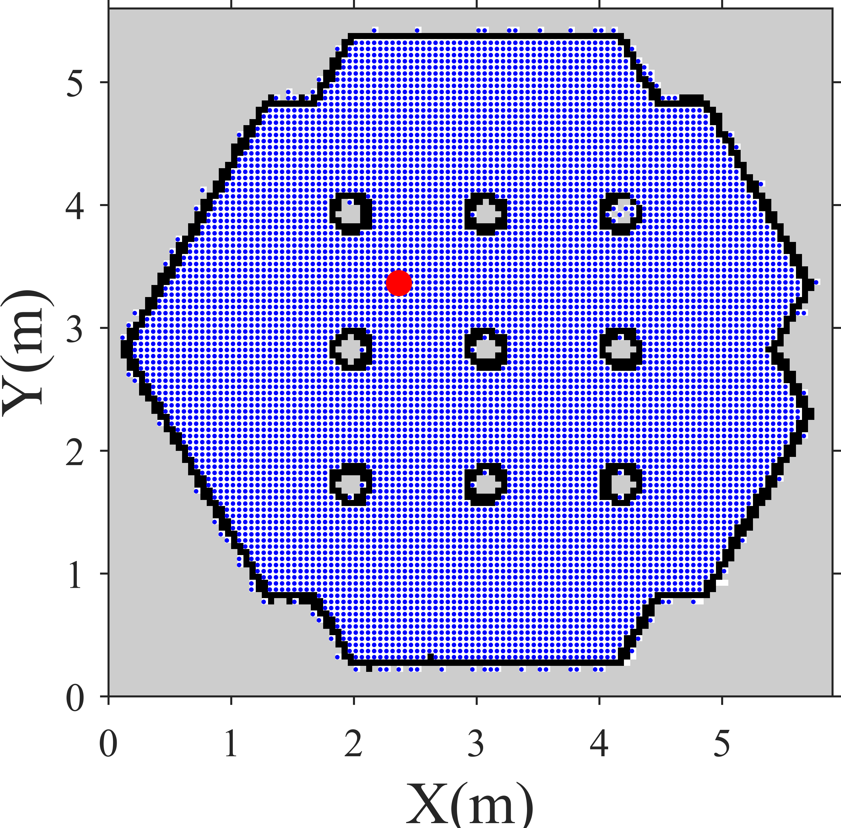
(a)

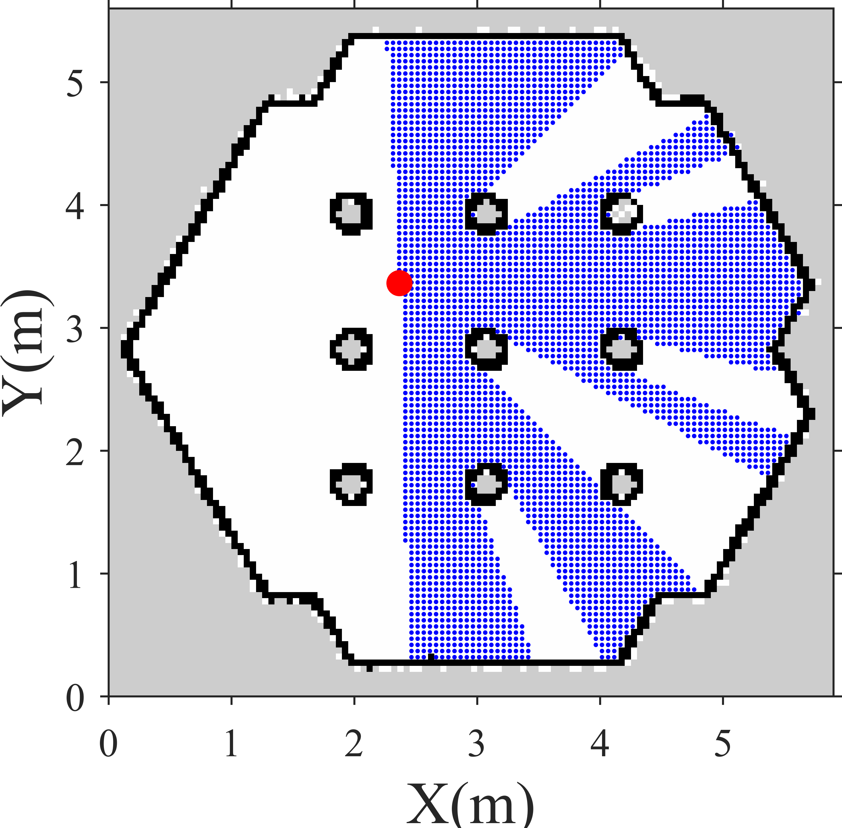
(b)

(c)

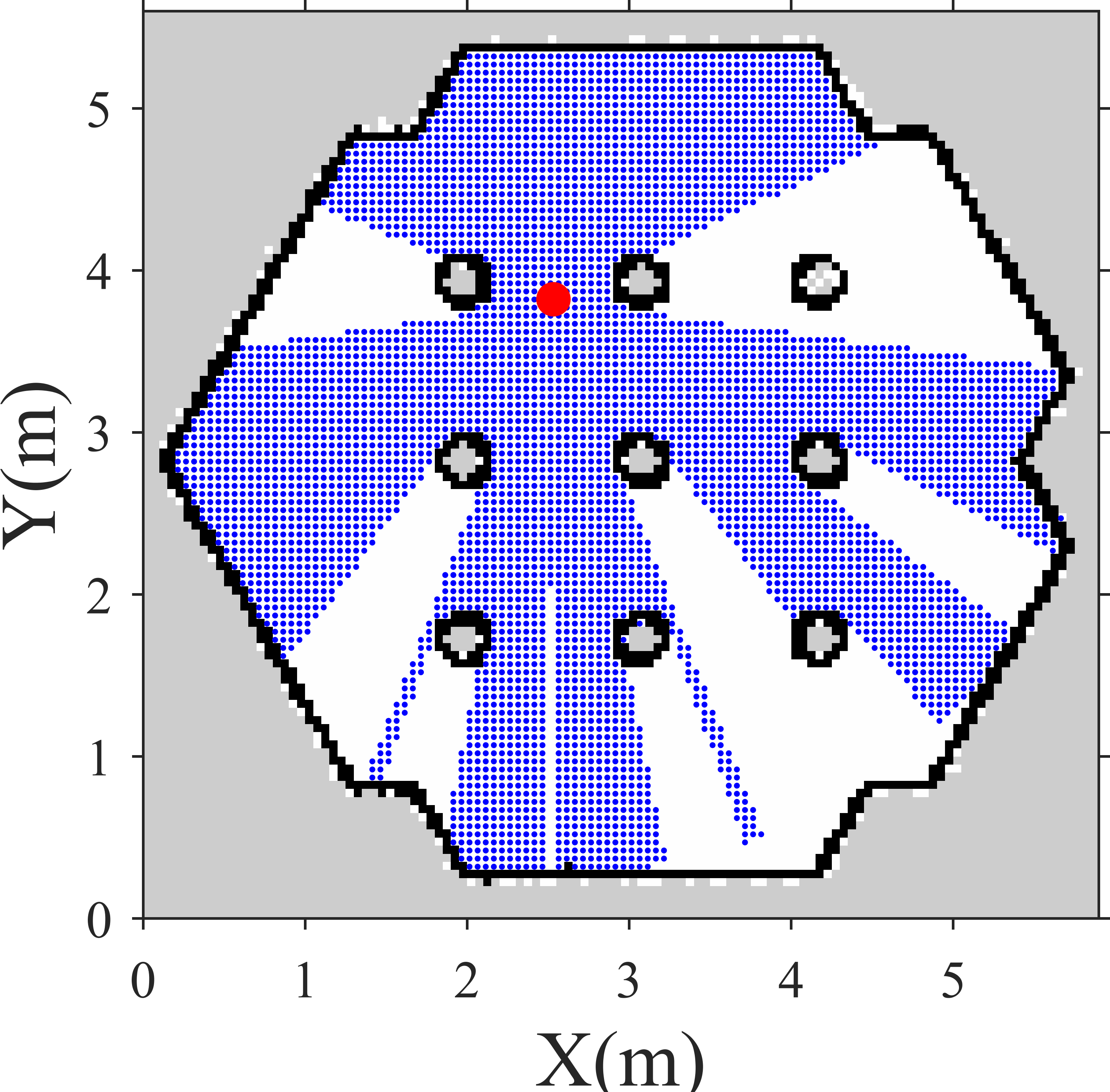
(d)

Figure 6: Mapping queried cells onto sensor data: (a) and (c) show all $Cell_{F}\in$ Query; (b) and (d) show all $Cell_{F}\in$ Query that underwent successful sensor mapping with 2 different sensors. Filled circle: sensor’s position in the map frame ($(X,Y)_{SM}$). Small dots: all the $Cell_{F}\in$ Query before and after sensor mapping.

3.3 Real-time computation technique for coverage calculation

This study has developed a real-time computation technique that utilizes descritized map data (via quadtree), sensor data, and matrix data structures for fast and accurate coverage rate calculation. The quadtree provides quick access (via querying) to all $Cell_{F}$ within the sensing range ($SR$) of the robot’s sensor at a time $t$. All $Cell_{F}\in$ Query are then mapped onto sensor data received at $t$ to match which $Cell_{F}\in$ Query is within the real sensor Field Of View ($FOV$) at time $t$. The coverage status of all $Cell_{F}\in$ Query which meet the matching are quickly stored to memory via matrices, and coverage is updated. All $Cell_{F}\in$ Query which do not meet this matching are dropped. Figs. 6(a)-(d) illustrate the process. Figs. 6(a) and (c) show all $Cell_{F}\in$ Query (with small dots). $SR$ is 3.5m, and is converted to cell length by multiplication with map resolution ($res$), so as to obtain the value of the querying radius as input for the quadtree algorithm. Figs. 6(a) and (b) correspond to a sensor with $FOV$ ranging from -1.57 to 1.57 radians and Figs . 6(c) and (d) represent the results for a sensor with $FOV$ ranging from 0 to 6.28 radians.

To perform the sensor data mapping, every $(X,Y)_{M}$ derived from all $Cell_{F}\in$ Query must be transformed to coordinate points in the sensor frame using a $TF_{MS}$. This is so to obtain an accurate coverage from the $FOV$ provided by the sensor. The $CoverageCalculator$ function (Algorithm 4) continuously calculates $tc$ and publishes the $(X,Y)_{zone}$ of least covered zones until $dc$ is reached. The reasons for this loop structure are as follows. (1) The relationship between the map frame and sensing frame (i.e., $TF_{MS}$) changes constantly as the robot moves around. Therefore, Algorithm 4 must continuously receive new $TF_{MS}$ information. (2) All the information provided to Algorithm 4 at each iteration must be time synchronized to ensure accurate coverage. This means that sensor data and the sensor position in the mapframe ($(X,Y)_{SM}$) at the time $t$, at which sensor data was received, are fed to Algorithm 4. $TF_{MS}$ is time synchronized with this data as well. This way, Algorithms 4 and 5 are able to accurately recreate the $FOV$ at a specific $t$. In subsection 3.3.1, all time synchronized data will be designated a subscript of $t$. The time interval between each iteration of Algorithm 4 is so minuscule that Algorithm 4 provides virtually continuous coverage calculation even at robot speeds of 5 m/s at an $SR$ of 3.5 m (to be discussed in section 4).

3.3.1 Algorithm flow

The $CoverageCalculator$ function (Algorithm 4) receives $TF_{MS_{t}}$ (published by the $tf$ package) and sensor data (published by the $sensor\_msgs$ packages). The sensor data is published as a data field [sensor_msgs/LaserScan.msg, 2023].

$$\alpha=\texttt{int}(\tan{\frac{Y_{S}}{X_{S}}\times\frac{180}{\pi}})\mod 360$$ (8)

This data field contains the following information: (1) The array ($SC_{a}$) which contains the values of the scan angles of the sensor, and (2) the array ($SC_{r_{t}}$) which represents the scan range associated with each scan angle. It is important to note that the scan angles are converted from radians to degree values which are then rounded down to the nearest integer (similar to the method seen in Eq. (8). This enables matching of the orientations of cells to the scan angles. The $CoverageCalculator$ function (Algorithm 4) uses the sensor’s position in the mapframe ($(X,Y)_{SM_{t}}$), $TF_{MS_{t}}$, and $SC_{r_{t}}$ as inputs. Algorithm 4 provides all $Cell_{F}\in$ Query, $TF_{MS_{t}}$, and $SC_{r_{t}}$ as inputs to the $Worker$ function (Algorithm 5). The $Worker$ function utilizes $TF_{MS_{t}}$, $SC_{a}$, and $SC_{r_{t}}$ to map each queried cell.

A cell is successfully mapped by meeting two criteria. First, the orientation ($\alpha$; calculated via Eq. (8)) is within the scan angles of the robot’s sensor. $\alpha$ is the orientation of the point coordinate of the cell ($(X,Y)_{S}$) in the sensor frame. On passing the first criteria, the second criteria involves the distance ($dist$) of the $(X,Y)_{S}$ of cell from the sensor. This distance should be less than the scan range at the corresponding scan angle. All cells which successfully pass the two criteria are accounted to memory using the storage matrix $M_{C}$. The $M_{C}$ matrix stores the coverage status and zone identification of every $Cell_{F}$ in the occupancy-grid map in order to ensure that covered cells aren’t counted twice and the coverage of each cell counts towards the coverage of the zone assigned to it.

$$M_{Z}(zid,4)=\frac{M_{Z}(zid,3)}{M_{Z}(zid,2)}\times(100)$$ (9)

$$\mathrm{Total\ Coverage\ rate}\ (tc)=\frac{\sum_{n=0}^{n_{z}-1}M_{Z}(n,3)}{\text{Total number of }\textnormal{Cell}\textsubscript{F}(\in\text{\small Occupancy-grid map})}\times 100$$ (10)

Algorithm 6 *

Algorithm 4: $CoverageCalculator()$

1:  while $Total\ Coverage\ rate<dc$ do

2:     $|TF_{MS},(X,Y)_{SM},\ sensor\ data|_{at\ time\ t}\leftarrow$ ROS tf and sensor$\_$msgs package

3:     Query every $Cell_{F}$ within $SR$ of $(X,Y)_{SM_{t}}$ $\leftarrow$ Requires use of Eq. (6) and converting $SR$ from meters to cell length

4:     $Worker(TF_{MS_{t}},all\ Cell_{F}\in Query,sc_{a},sc_{r_{t}})$

5:     Find zones with the minimum $c_{z}\leftarrow M_{Z}(:,4)$

6:     If there is more than one such zone, choose the zone of smallest $d$

7:     Share chosen zone’s centroid information to $ArnoldTrajectoryPlanner$

8:     $tc\leftarrow$ Eq. (10)

9:     if $tc\ \geq\ dc$ then

10:        $Stop$

11:     end if

12:  end while

Algorithm 7 *

Algorithm 5: $Worker(TF_{MS_{t}},all\ Cell_{F}\in Query,sc_{a},sc_{r_{t}})$

1:  for $Cell_{F}\in Query$ do

2:     $ind\leftarrow$ Eq. (3)

3:     if $M_{C}(ind,2)==\ 0$ then

4:        $(X,Y)_{M}\ of\ Cell_{F}\leftarrow$ Eq. (4)

5:        $(X,Y)_{S}\ of\ Cell_{F}\leftarrow dotproduct(TF_{MS},(X,Y)_{M})$

6:        $\alpha\leftarrow$ Eq. (8)

7:        if $\alpha\in SC_{a}$ then

8:           $dist\leftarrow$ distance between sensor and $(X,Y)_{S}$

9:           if $dist\ <sc_{r_{t}}\ at\ \alpha$ then

10:              $M_{C}(ind,2)=1$

11:              $zid\leftarrow M_{C}(ind,1)$

12:              $M_{Z}(zid,3)+=1$

13:              $M_{Z}(zid,4)\leftarrow$ Eq. (9)

14:           end if

15:        end if

16:     end if

17:  end for

Each row of $M_{C}$ stores information about an individual $Cell$. The columns of $M_{C}$ contain the following information from left to right: index ($ind$) values of all cells in the occupancy-grid map, zone identifier ($zid$), and coverage status. It should be noted that: (1) all $Cell_{O}$ and $Cell_{U}$ are not assigned any zone identifiers, (2) every $zid$ represents a row of $M_{Z}$, and (3) the coverage status column keeps account of all $Cell_{F}$ which have been accounted for. Each cell has a column value of 0 when unaccounted, and a value of 1 when accounted. This column continuously updates itself as the program runs. Once a cell’s coverage status is updated in $M_{C}$, zone’s coverage rate ($c_{z}$) is also updated in storage matrix $M_{Z}$ (using Eq. (9)). Algorithm 4 then uses the fourth column of $M_{Z}$ to calculate the total coverage rate ($tc$) (see Eq. (10). Algorithm 4 is continuously invoked in a loop until $dc$ is reached, at which point Algorithm 4 communicates to Algorithm 1 to shut down. Algorithm 4 also shuts down as well.

4 Experiments and Results

To validate the proposed methods described in this paper, we conducted three experiments. (1) We compared the total coverage time ($CT$) of developed CCPP application to that of the more established CPP method, boustrophedon coverage path planning (BCPP). These tests were carried out in three simulated environments of varying size, shape, and obstacle density. The robot used in these tests was a Turtlebot3 with a 2D LiDAR ($FOV$ ranging from 0 to 6.28 radians). (2) We performed real-life testing of the algorithms in a classroom environment. The robot used in this test was a Turtlebot2 with a camera sensor (with a $FOV$ ranging from -1.047 to 1.047 radians). A video of the trial is available . And (3) we evaluated the computational speed of coverage calculation method. This experiment was carried out in a simulated environment. An additional experiment is also showcased at the end of this section to discuss the influence of parameters (specifically $n_{iter}$ and the number of zones) on coverage time. The source code of our CCPP application is available . All simulated and real-world environments contain only static obstacles.

4.1 Comparing performance of CCPP and BCPP applications

BCPP [Choset, 2000, Choset and Pignon, 1998] is a fairly common method for CPP used in various applications, such as cleaning [Ntawumenyikizaba et al., 2012], agriculture [Coombes et al., 2019], demining [Bähnemann et al., 2021], and multi-robot coverage [Rekleitis et al., 2008]. The primary reasons for using BCPP for comparison are as follows. (1) Using a widely researched method in the field of CPP will provide a good benchmark for our method’s performance. (2) There are open-source BCPP applications available for this comparison [ethz-asl / polygon_coverage_planning github, 2023, Rjjxp/coverageplanning github, 2023, Gonzalez et al., 2005, Bormann et al., 2018, Gomez et al., 2017, Greenzie / boustrophedon_planner github, 2023, Ipiano / coverage-planner github, 2023], compared to other methods used in CPP, which are not publicly available to our knowledge. Boustrophedon planning is a method for generating a path for a robot that alternates back and forth across an area. This planning is usually paired with cell decomposition, a technique used to divide a 2D space into simple polygons (cells). Boustrophedon planning and cell decomposition are aptly named boustrophedon cellular decomposition. Each cell represents free space. The boustrophedon paths generated to cover each cell is guided by the shape of the obstacles and boundaries surrounding said cell. The boustrophedon cellular decomposition method, unlike our on-line CCPP method, is therefore an off-line coverage path planning technique that requires full prior knowledge of the size and shape of the environment and all obstacles within.

4.1.1 Comparing coverage times

To compare the performance of our CCPP method with that of BCPP, this study used the BCPP application developed in ROS and provided in [ethz-asl / polygon_coverage_planning github, 2023]; the accompanying paper is [Bähnemann et al., 2021]). It was difficult to operate the other open-source applications, and technical support from the contributors to those applications was lacking. It must be noted that the BCPP application used in this paper provides coverage times based on more theoretical calculations, as the coverage path plan created was not tested in a Gazebo simulation, similar to our CCPP application. The BCPP application therefore only provides a visual representation of the generated path and the calculated estimated coverage time. This means the BCPP application just shows what the path plan would look like based on the parameters. The coverage time is calculated (by the application) based on the generated path and the parameters. The procedure to provide this planned path to the simulated robot (in gazebo) to enact was not provided by BCPP algorithms. We consider three different environments shown in Fig. 7.

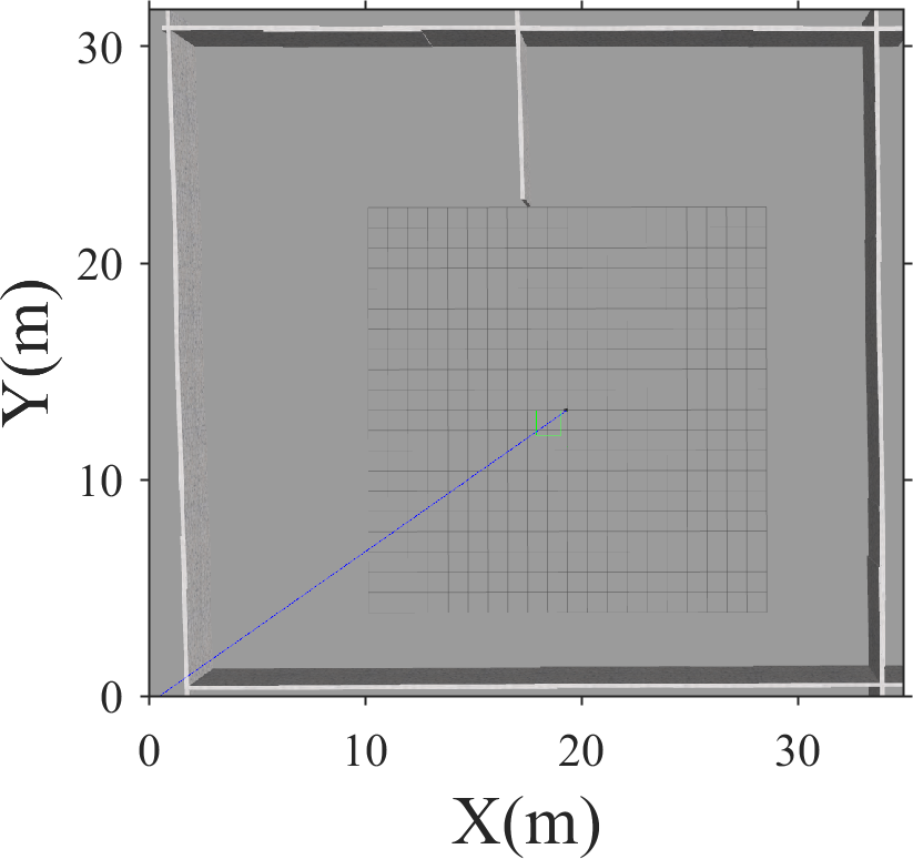
(a)

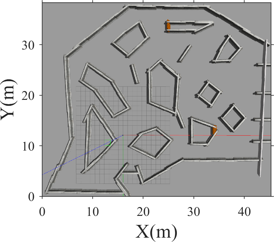
(b)

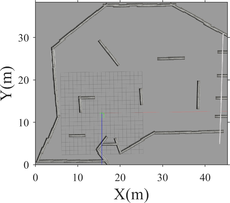
(c)

Figure 7: Simulated environments (a) Esquare, (b) Ldense, and (c) Hdense.

The environments are significantly larger than the robot’s size, to provide large areas to cover. These environments vary in size, shape and obstacle density to provide a varied range of scenarios for analysis. Fig. 7(a) shows a simple-shaped environment with one wall obstacle, while Figs. 7(b)-(c) show complex-shaped environments with sparse and high obstacle density, respectively. The names of these environments are: Esquare (fig. 7(a)), Ldense (fig. 7(b)), and Hdense (fig. 7(c)). To perform an accurate comparison, we have set the parameters for both applications to values that ensure: (1) both applications achieve an estimate of 100% coverage rate ($tc$) for each environment. This aspect of the experiment is further discussed later. (2) Both applications adhere to the same physical constraints placed on the Turtlebot3. And (3) $tc$ is achieved within a reasonable time frame.

Due to occasional inaccuracies in map generation during the SLAM, some of the obstacles are represented as containing free space. In other occasions, such spurious free space could be created outside the boundaries of the environment map. These inaccuracies occur as a result of bad sensor data. Any $Cell_{F}$ within these spurious free space could be covered during the coverage process. The compensation method for this issue will be discussed later in this section.

For both the BCPP and CCPP applications, we set the robot’s velocity to 0.22 m/s for all runs. To achieve coverage of all environments using BCPP, we set certain parameters (available in the configuration folder of the application) at constant values. These parameters are: (1) lateral overlap, which is set to 0 to maximize sweep distance and obtain the best possible coverage times; (2) maximum acceleration, set to 0.3 m/s² (the maximum acceleration of the Turtlebot3); and (3) wall distance, set to 0.2 m to account for the dimensions of the robot. The robot has a width of 0.173 m (its largest dimension). For the comparison, we varied the lateral footprint (LF) parameter for each environment. The lateral footprint parameter sets the sweep distance and is defined to be twice the sensing range ($SR$) with the robot’s center at the sweep line. With this choice, there would be no coverage overlap between sweeps; it allows optimized progressive scanning of unvisited areas for BCPP application. This ensures fair comparison between the two CPP applications. The actual total coverage after the BCPP operation is not shown in the program output. To this end, the lateral footprint is reduced as the map shape complexity and obstacle density increase, this is to ensure thorough coverage. The lateral footprint for Esquare, Ldense, and Hdense is 7.0 m, 4.0 m, and 3.0 m, respectively. Fig. 8 shows the BCPP coverage for different environments. Figs. 8(a)-(c) present the cell decompositions, and Figs. 8(d)-(f) showcase the robot’s sweep across the environments. All the maps in Fig. 8 were manually created in the application and are therefore a close representation of the actual maps (generated via SLAM). Some of the obstacles and the map boundaries have been slightly simplified to enable computation of polygons. The ”S” and ”G” icons shown in green and red are the start and stop positions of the sweeps.

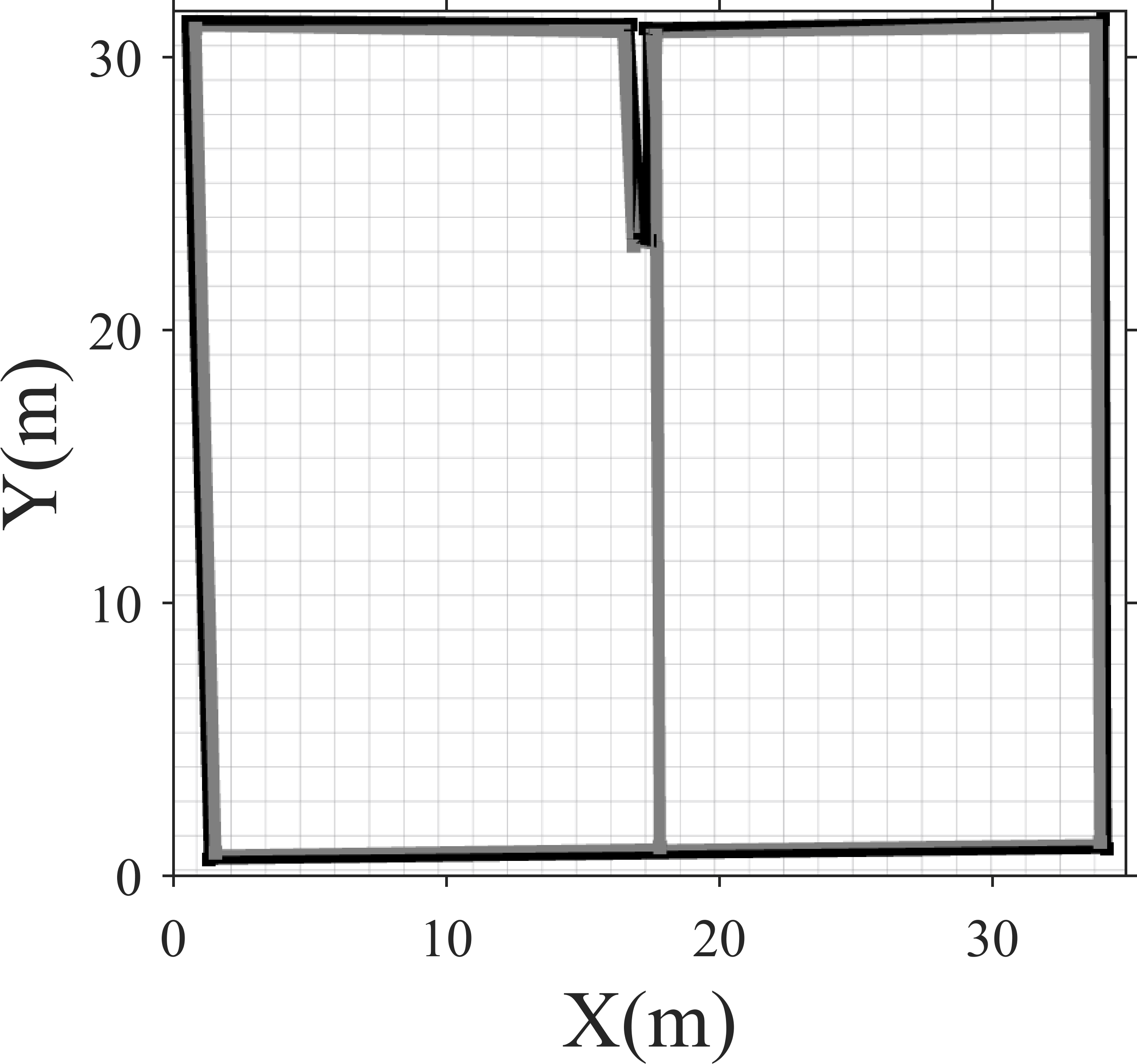
(a)

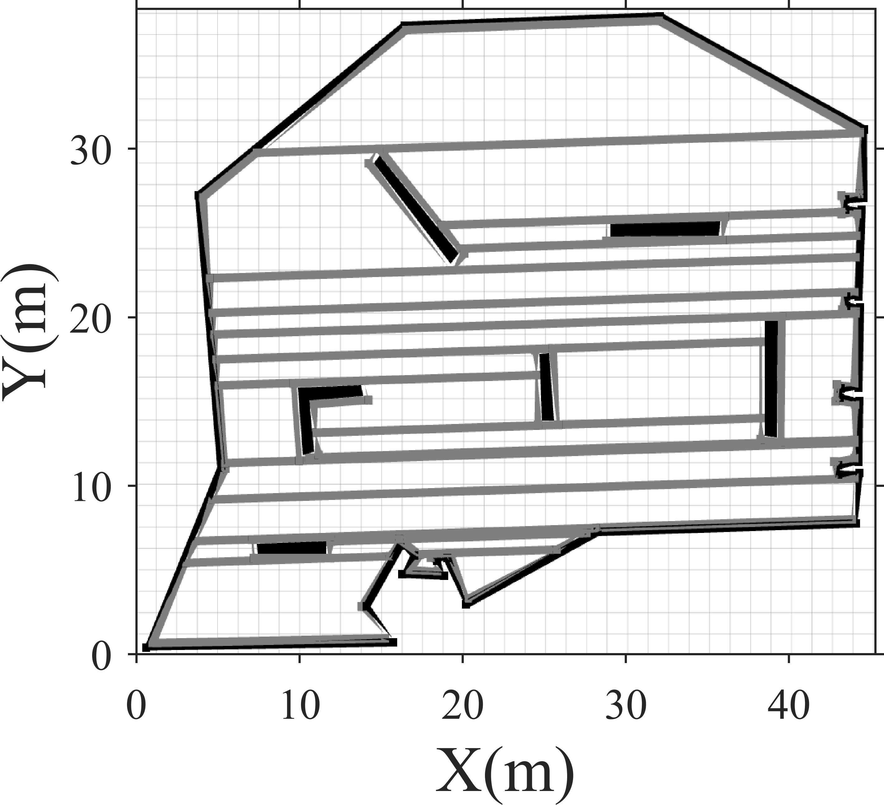
(b)

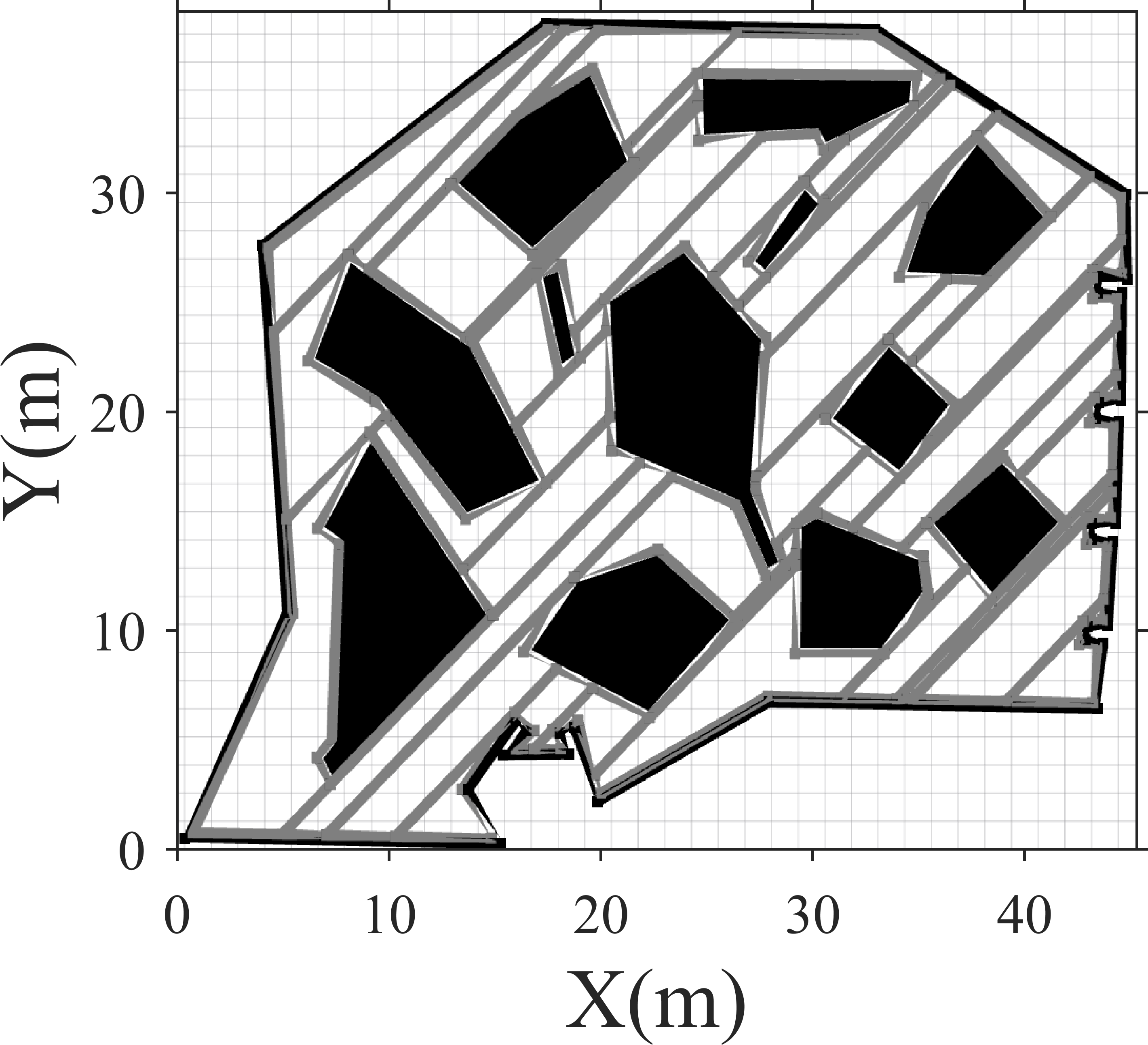
(c)

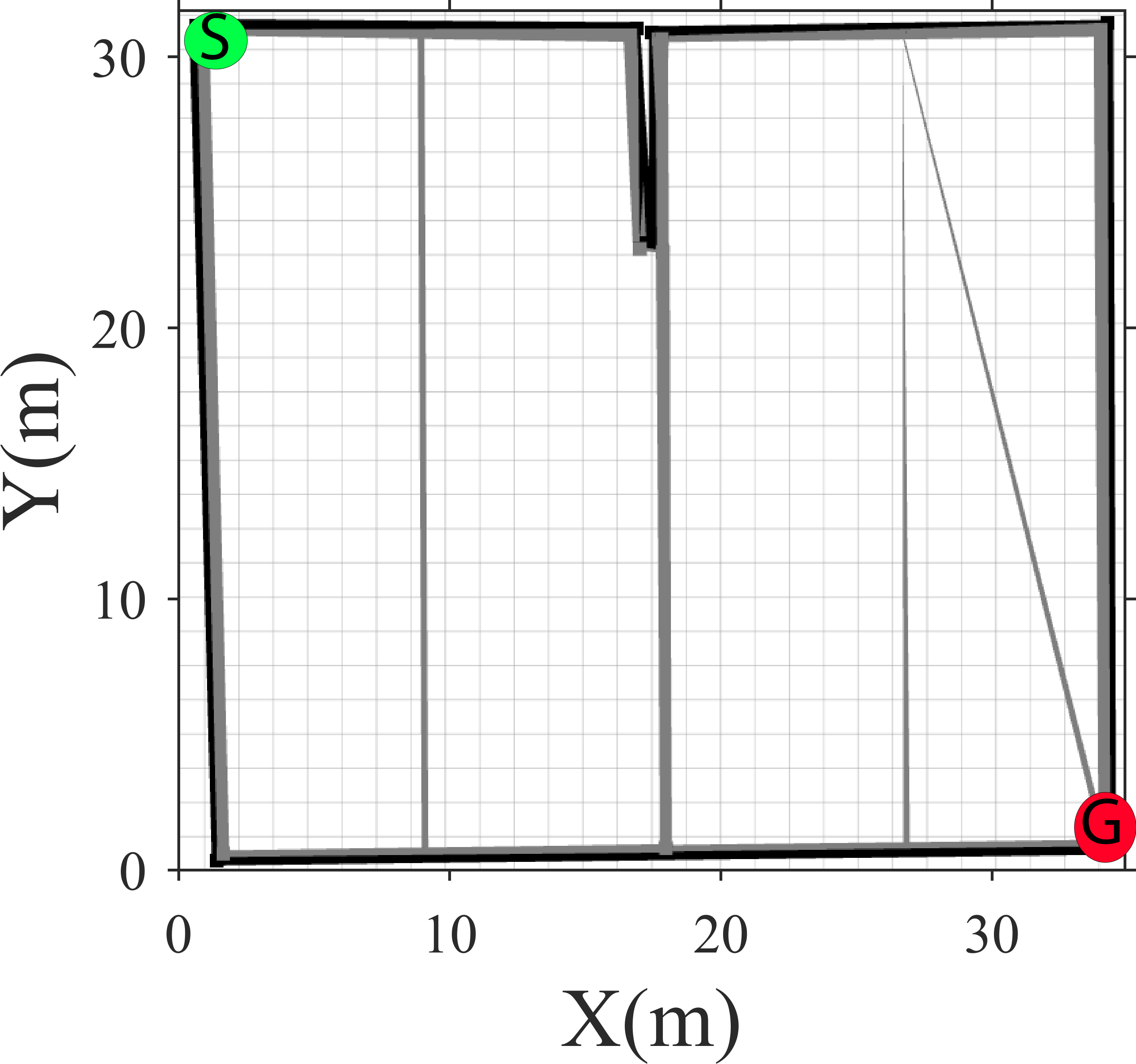
(d)

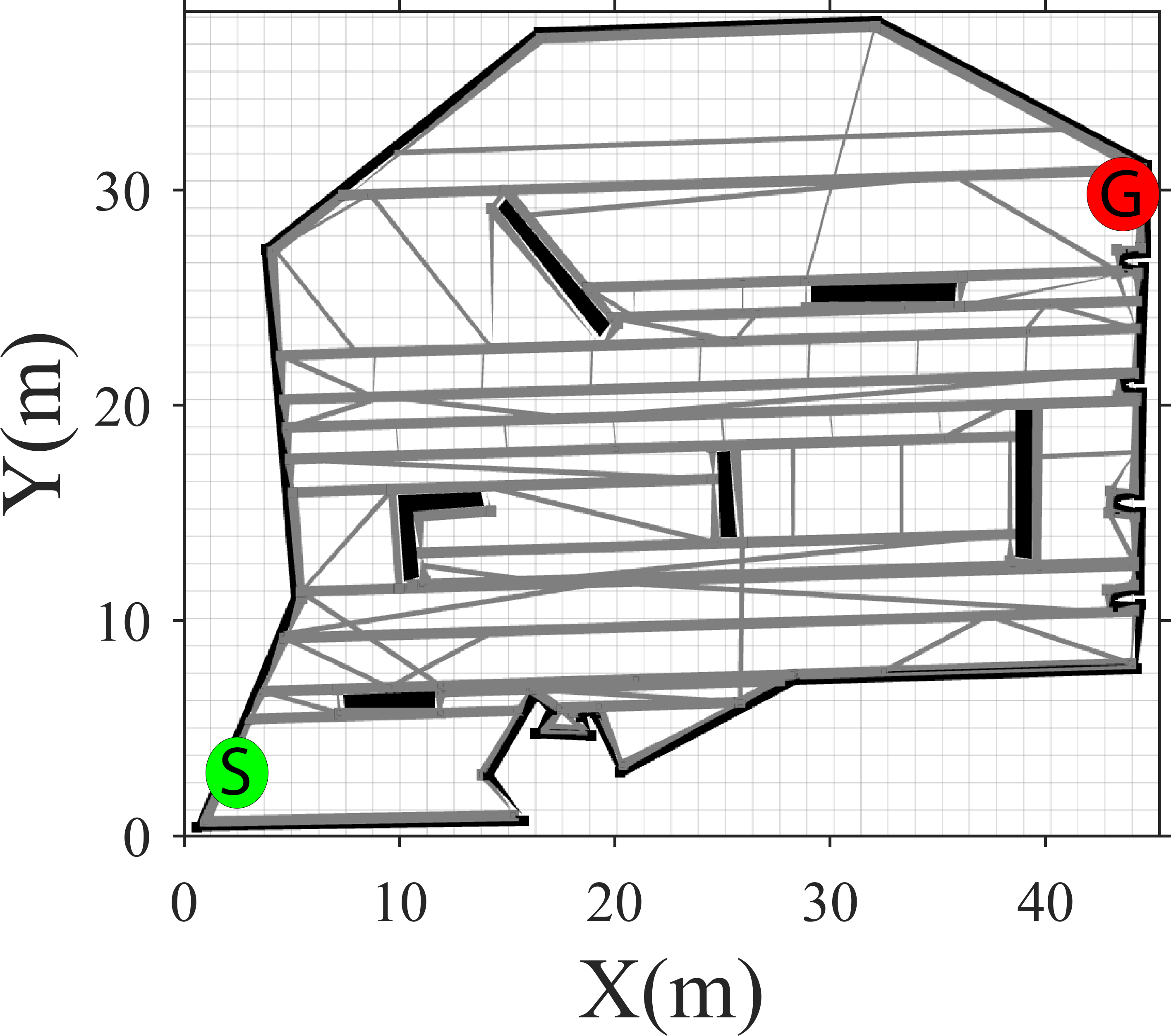
(e)

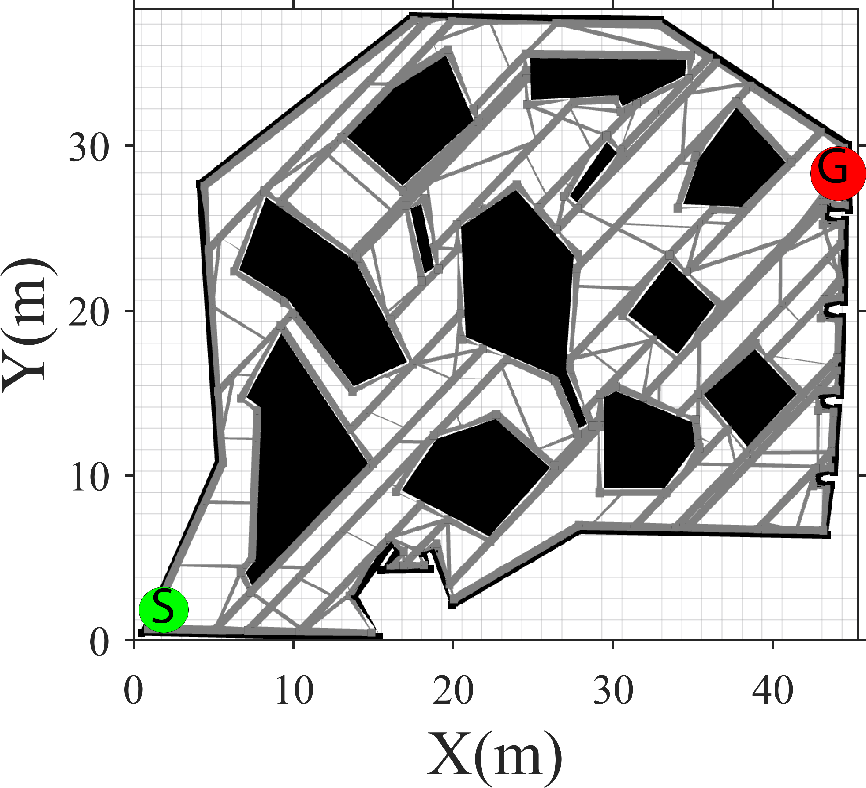
(f)

Figure 8: Coverage of simulated environments using BCPP: (a)-(c) the cellular decomposition of the maps, and (d)-(f) the planned boustrophedon coverage path.

Fig. 9 shows the coverage across these same environments using CCPP. For CCPP, the start position of the robot in each environment is kept the same as those used in the BCPP application for accuracy. As discussed, the SR used for each environment in CCPP application is half of the lateral footprint chosen for BCPP applications. The parameter values of zones, $n_{iter}$ and $n_{s}$, were chosen by trial and error. These parameters provided the smallest coverage times out of all the trial runs. Figs. 9(a)-(c) and 9(d)-(f) show the chaotic trajectories and covered cells for each environment, respectively. For the CCPP application, the desired coverage rate ($dc$) for every environment is set to approximately 97% for the following reasons. (1) As discussed, the $tc$ of the BCPP operation is not outright provided as part of the output. It is difficult to visually discern the completeness of coverage. For more complex-shaped maps, $tc$ might not be 100% as a result of the simplified polygons used to describe the obstacles. This aspect of performance drop off of BCPP is further discussed in section 4.2. (2) By selecting a slightly lower $tc$ than 100%, we aim to compensate for the previously discussed map inaccuracies during the SLAM that leads to account non-existent free space in coverage calculations in the CCPP algorithms. And (3) the CCPP application shares the same difficulty in reaching a $tc$ of 100% as chaotic trajectories cannot be fully controlled.

Table 1: Performance of BCCP and CCPP in various maps.

Map	Approx. $Area_{F}$ ($m^{2}$)	$SR$ (m)	LF (m)	$n_{iter}$	$ns$	no. of zones	$CT_{BCPP}$ (min)	$CT_{CCPP}$ (min)	$ratio_{CT}$
Esquare	1010.44	3.5	7.0	20	20	40	13.22	39.28	2.97
Ldense	1217.47	2.0	4.0	20	20	60	43.71	101.08	2.31
Hdense	895.18	1.5	3.0	20	20	90	47.52	92.37	1.94

Table 1 compares the coverage time ($CT$) for BCCP and CCPP in different maps. At the parameters chosen, our CCPP is approximately 2.97, 2.31, and 1.94 times slower than the BCPP application for Esquare, Ldense, and Hdense environments, respectively. The results indicate reasonably comparable performance of CCPP and BCPP, specially in moderately and highly cluttered environments. Nevertheless, it is important to consider the following factors when comparing the two methods. In general the BCPP can exert more control over the trajectories for two reasons. (1) There is a prior knowledge of the dimensions and shapes of the boundaries and obstacles of the environments which enables effective path tracing within cells. (2) The application uses a start and a goal position to generate an overall coverage path plan which minimizes repeated coverage as the robot journeys from cell to cell, therefore optimizing the coverage time ($CT$). These attributes of BCPP result in the creation of a more absolute predetermined coverage path plan with very little wasted robot motion. Additionally, the BCPP application has lateral footprint and lateral overlap parameters that enable optimization of progressive coverage. This along with the ability to plan the entire coverage path provides a significant control of amount of coverage overlap as the robot moves around. Our CCPP application does not have have such parameters to fully control the coverage overlap. Other than the techniques we used to disperse the chaotic trajectories and avoid the obstacles, this work does not employ any other forms of trajectory control. It must also be accounted that the BCPP application used in this paper provides a more theoretical coverage time. The $CT$ might be more or less than what was calculated if a robot (in Gazebo or real-life) traveled the generated paths.

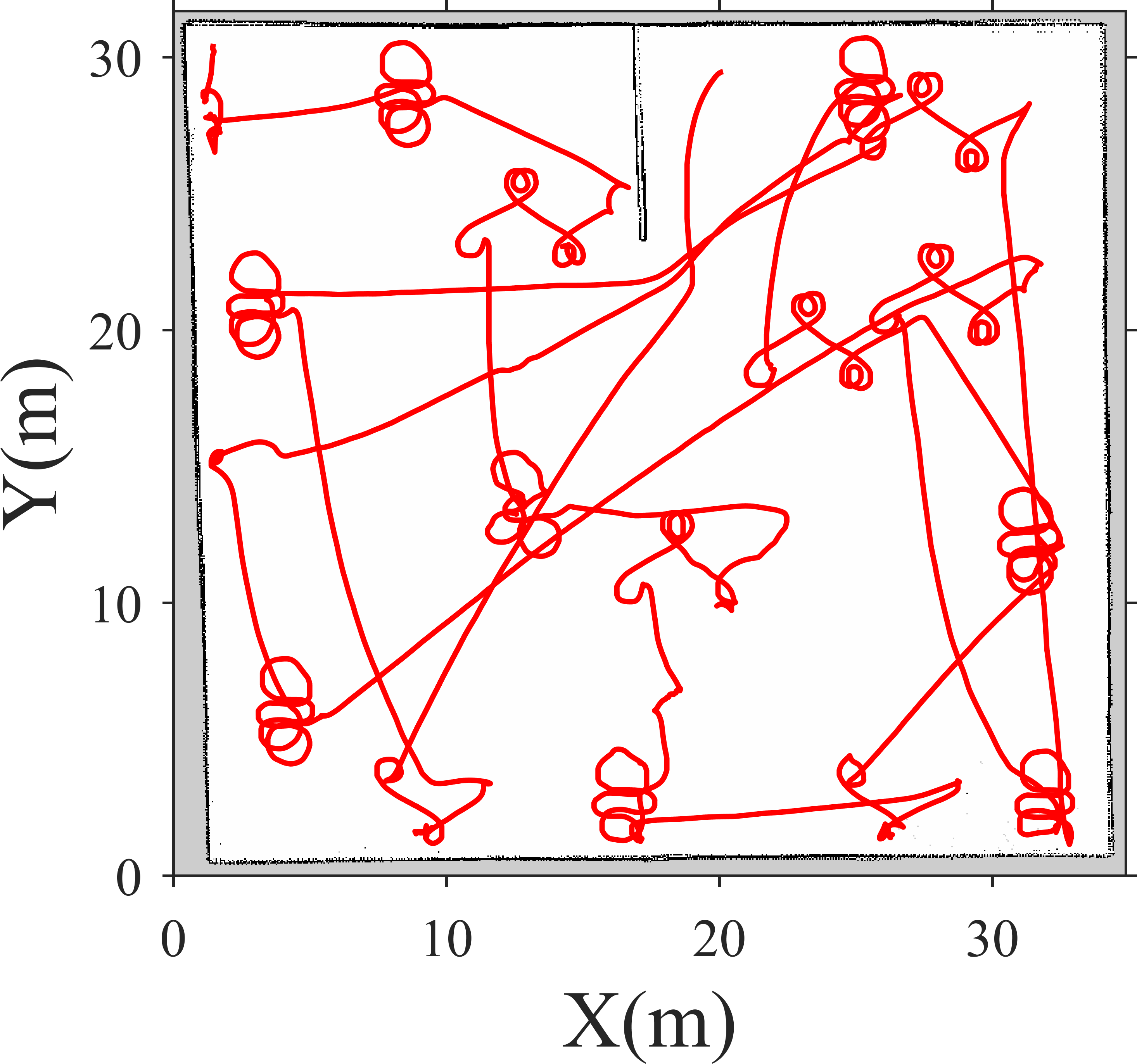
(a)

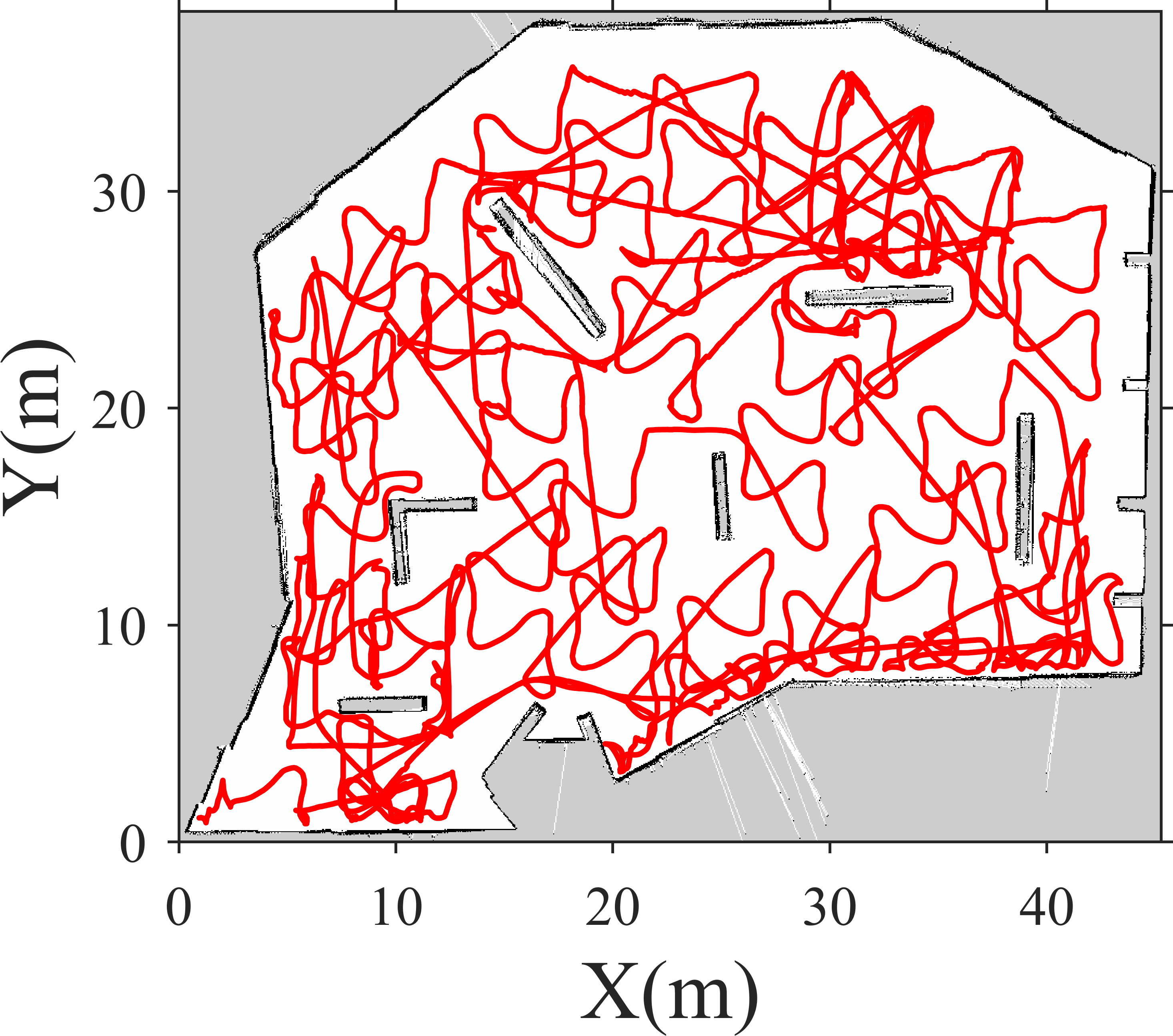
(b)

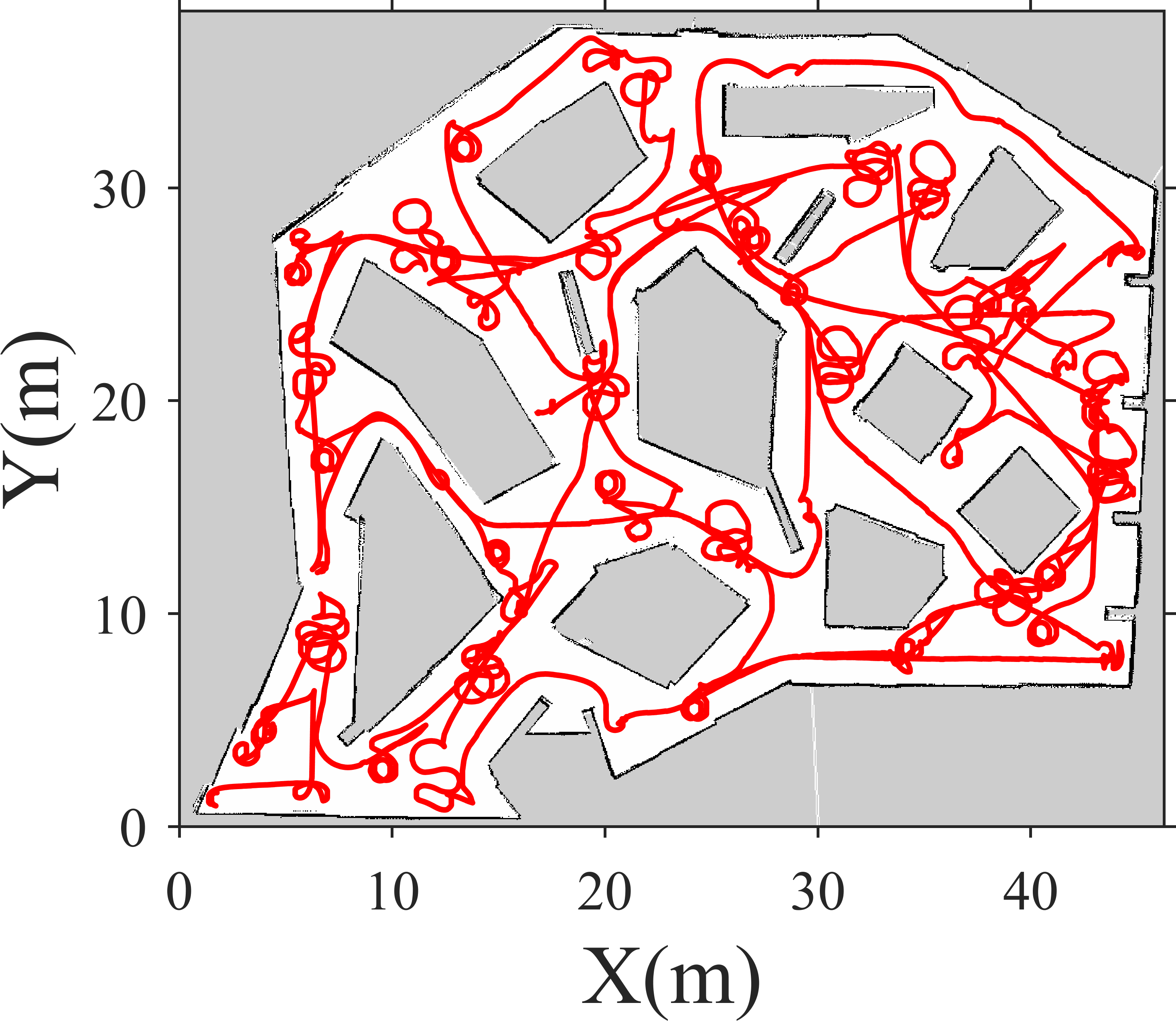
(c)

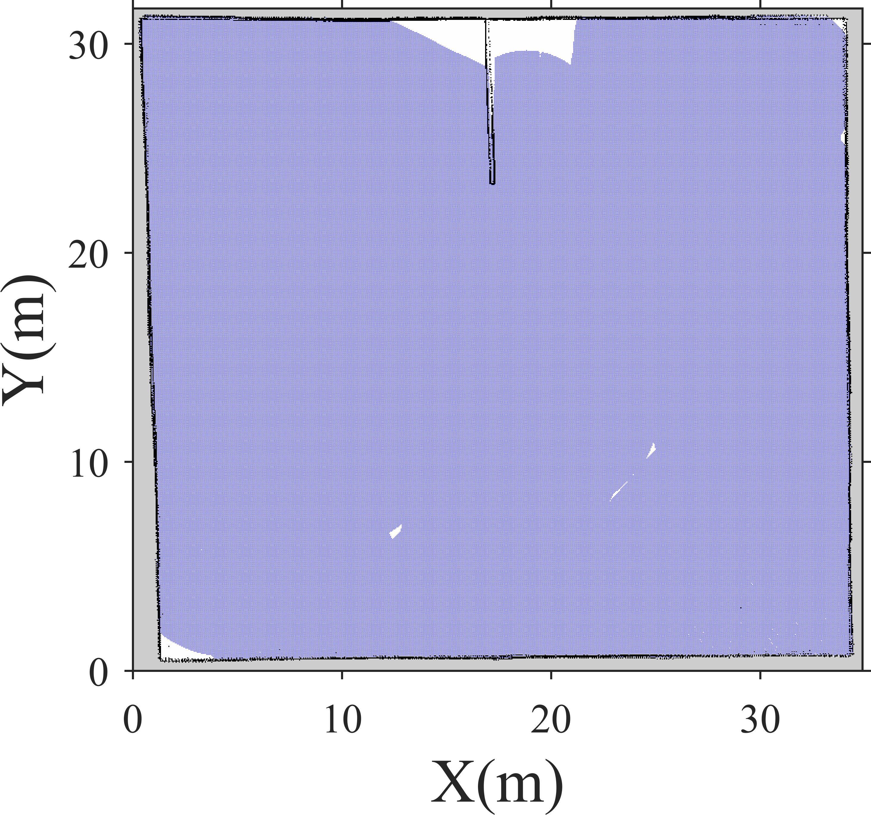
(d)

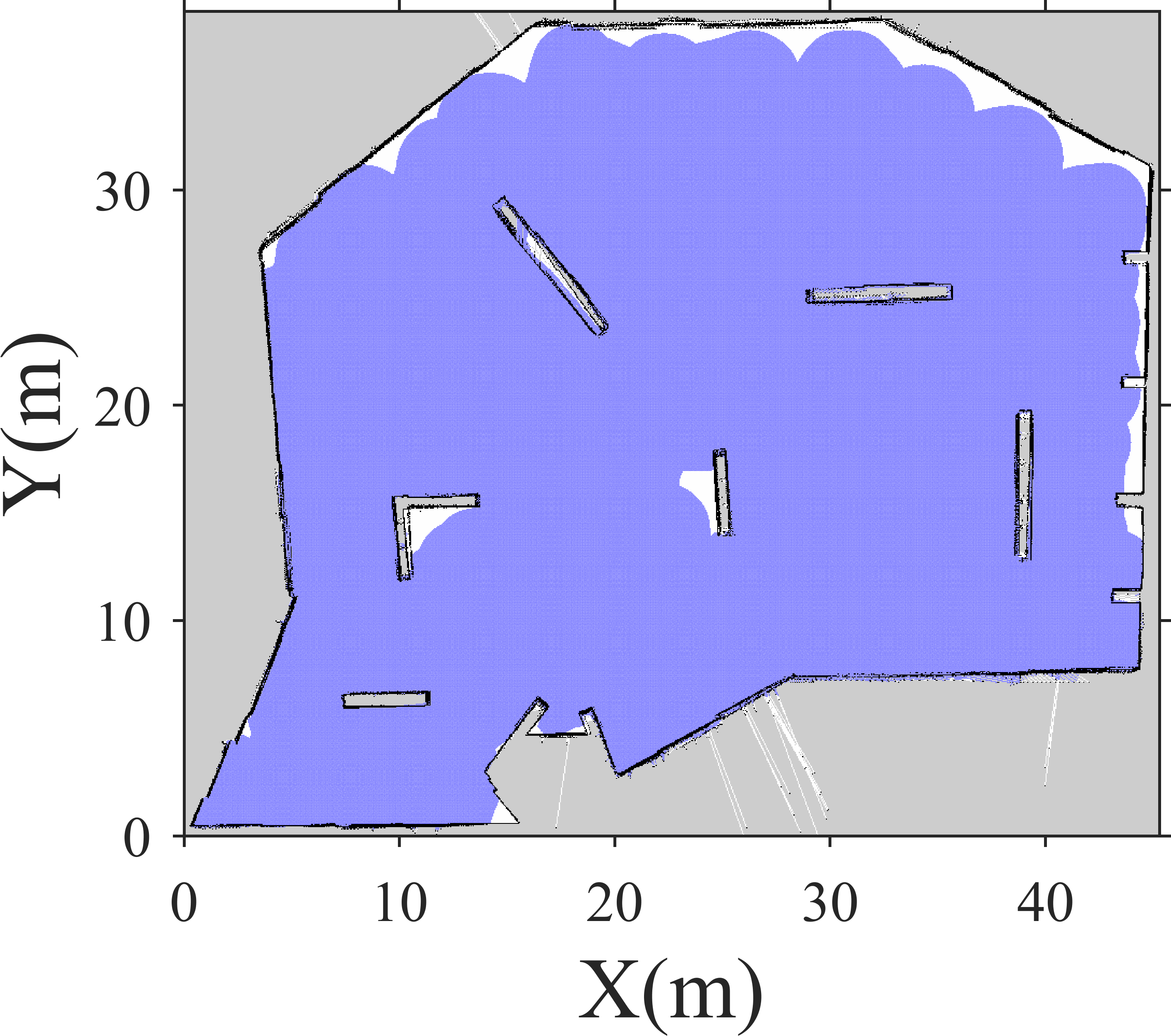
(e)

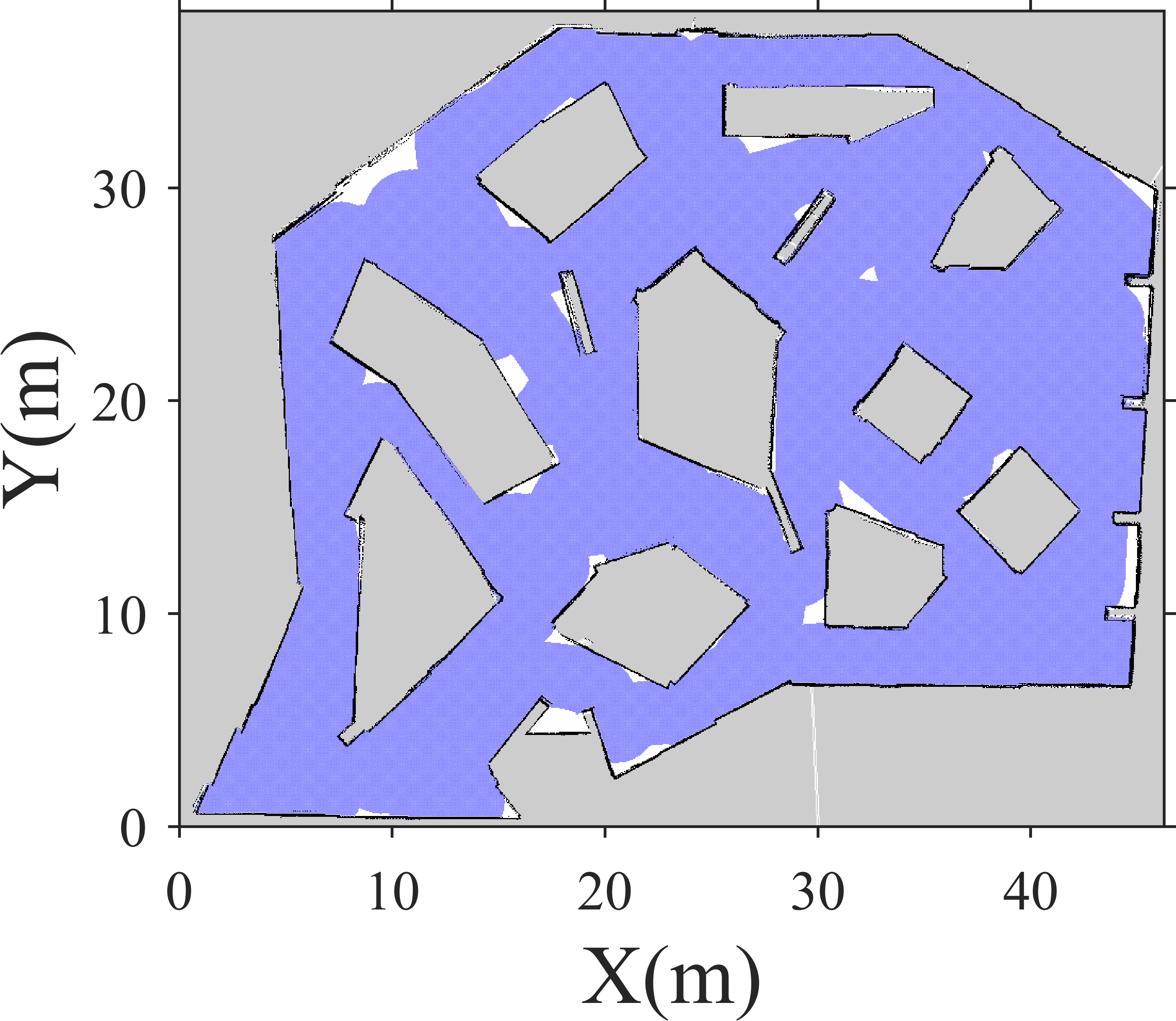
(f)

Figure 9: Coverage of simulated environments using CCPP: (a)-(c) chaotic trajectories, and (d)-(f) covered cells.

Additionally, the CCPP corresponds to longer coverage times as the method must balance between two goals (as opposed to just one in BCPP): maintaining unpredictable movement and providing desired coverage. Lastly, it is perhaps possible that a different set of parameters not tried here would have brought the coverage times closer to those of the BCPP application.

Lastly, we ran a comparison using the maximum $SR$ of the simulated turtlebot3 lidar in Hdense. Figs. 10 (a) and (b) showcase an example of potentially reduced BCPP performance. In this result, the BCPP application covers the Hdense environment in 33.56 minutes with a lateral footprint of 7.0 m. There is a 29.40% drop in $CT$ using a lateral footprint 7m as opposed to 3m (Figs. 8(c) and (f)).

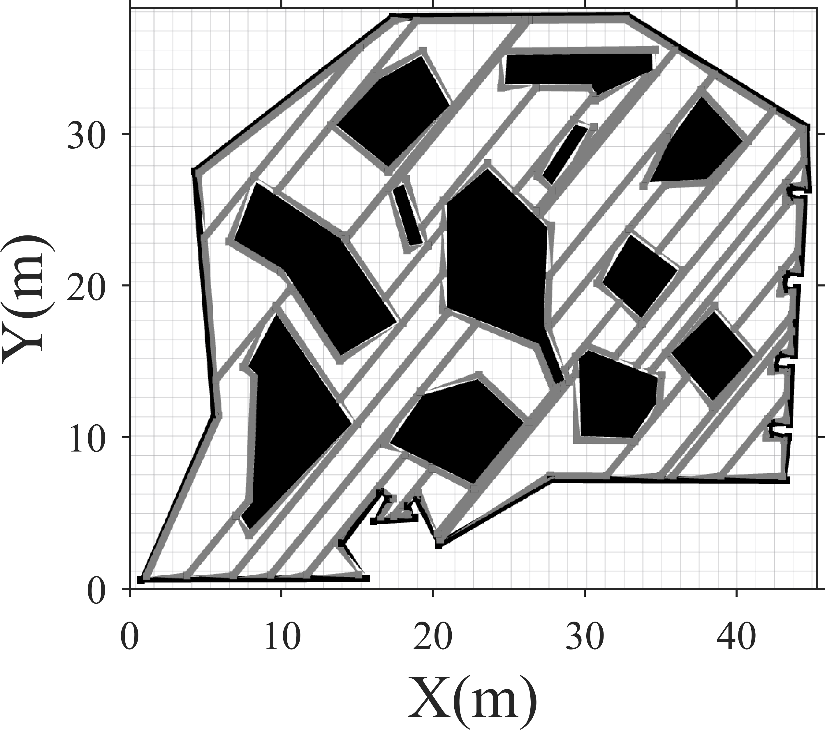
(a)

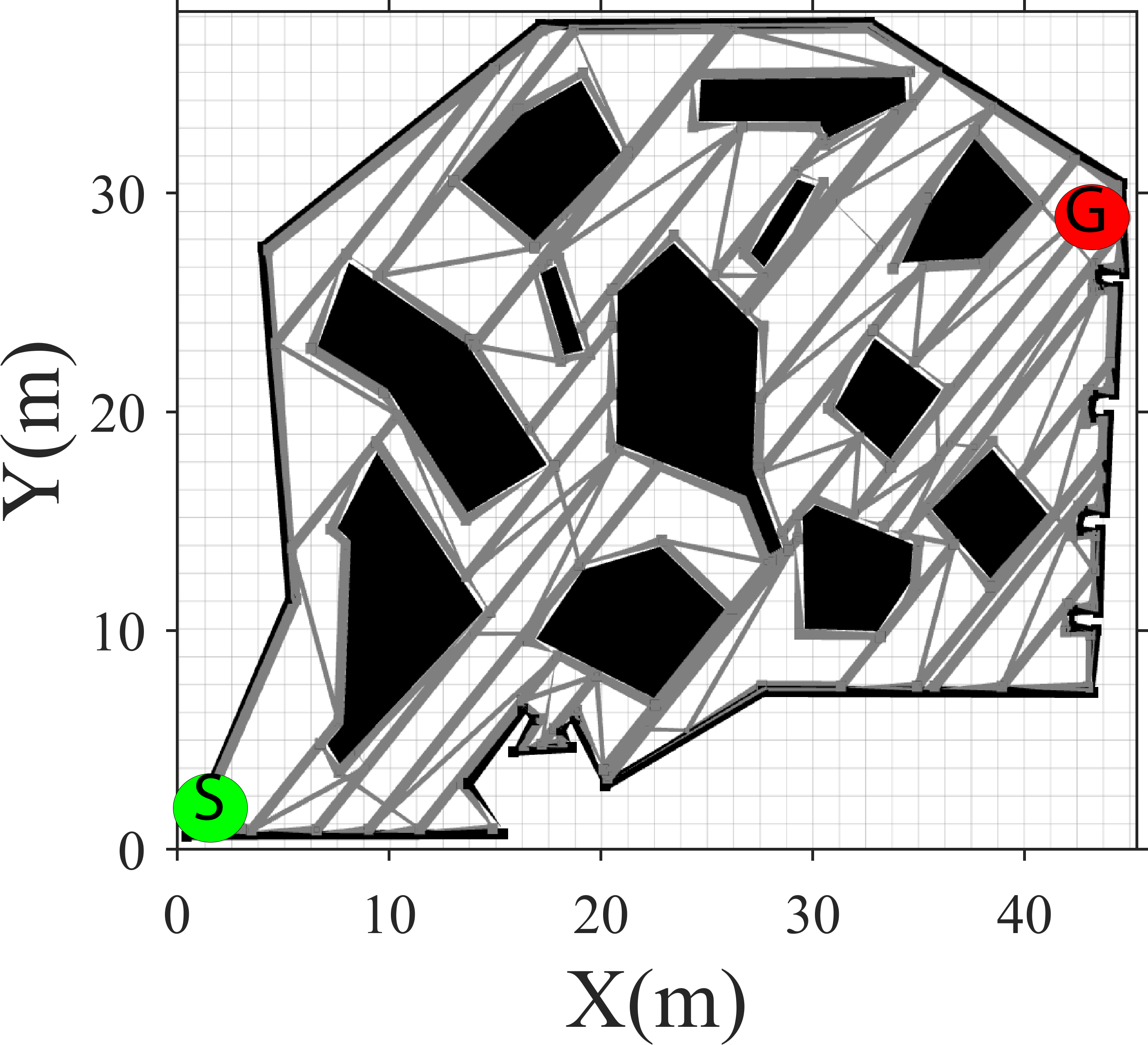
(b)

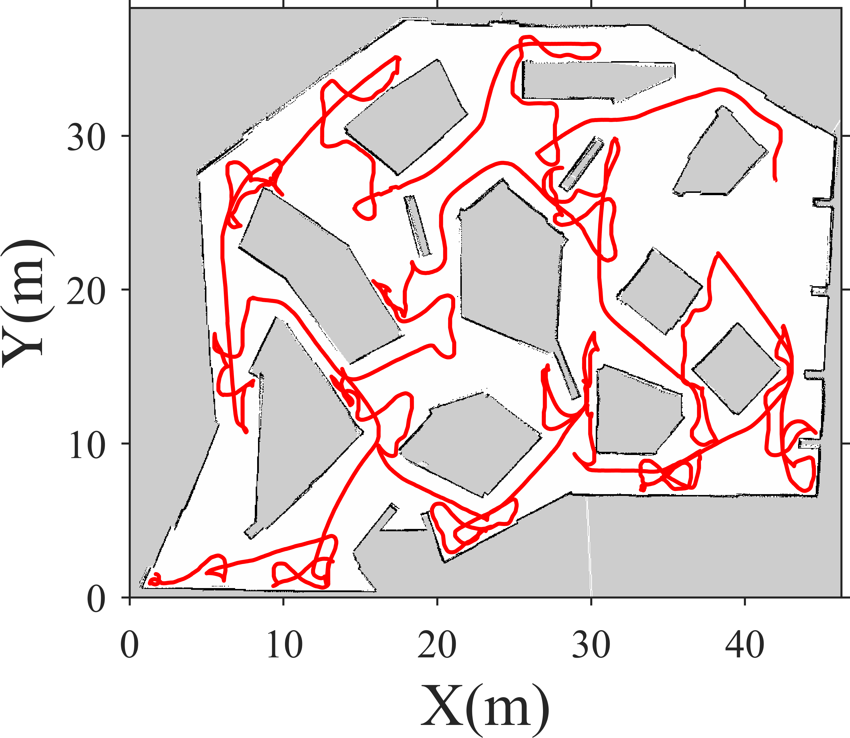
(c)

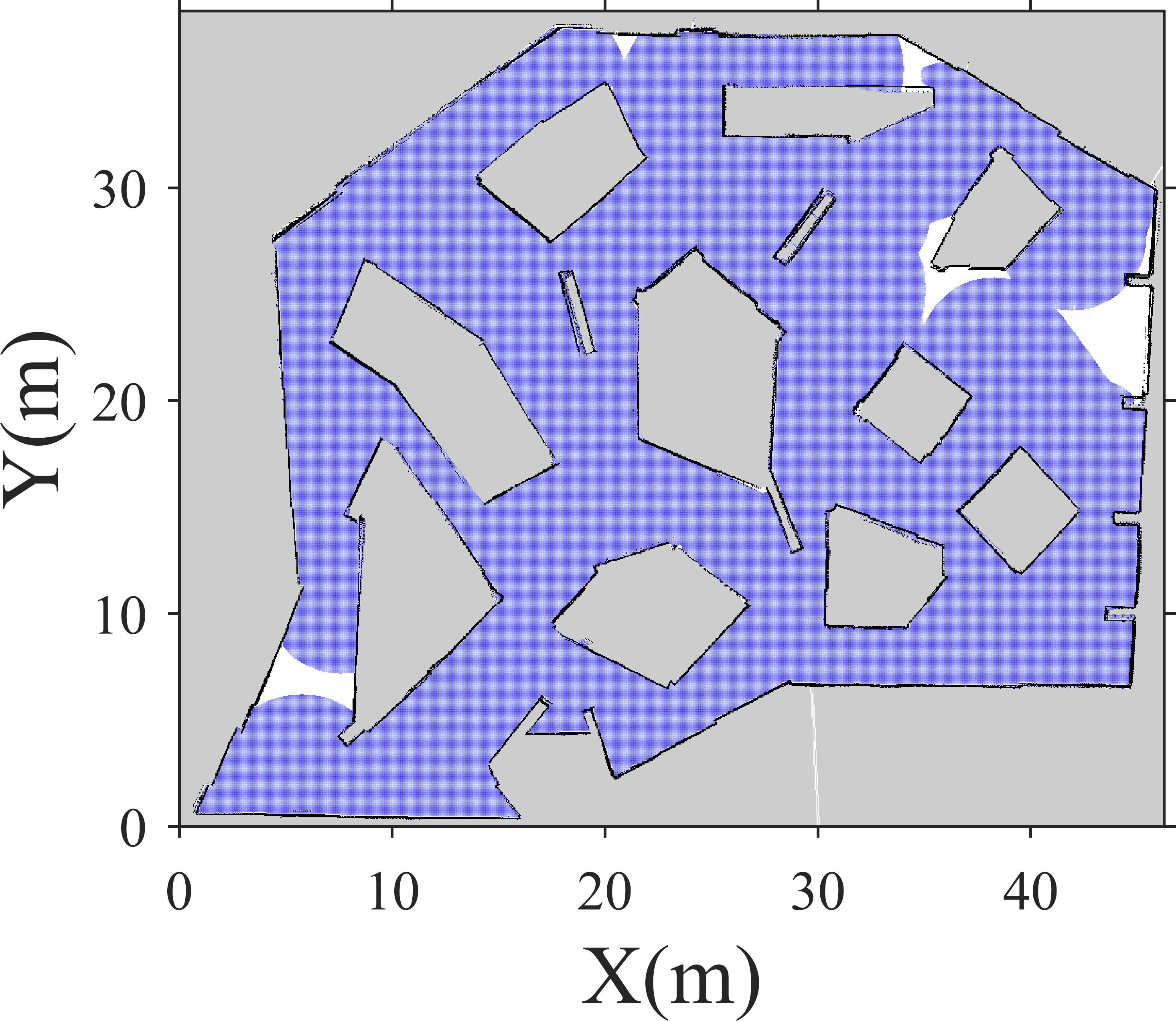
(d)

Figure 10: The BCPP and CCPP application used in Hdense: (a-b) shows cellular decomposition and planned boustrophedon coverage path. (c-d) shows chaotic trajectories and covered cells.

Figs. 10 (c) and (d) showcase the performance of our CCPP in the Hdense environments at 97% coverage. The $SR$ was 3.5 m and the $CT$ was 44.24 minutes at parameter values set in Table  1. There is a 56.23% decrease in $CT$ at this $SR$ from the CT using $SR$ of 1.5m (Figs. 9(b) and (e)). Section 4.2 will further discuss the performance the potential advantages of our CCPP method and problems that arise when BCPP faces worst case scenario computational complexity issues as well as some additional problems thereof.

4.2 Potential advantages of CCPP over BCPP

When it comes to sensor based coverage applications, our CCPP method might be more adaptable to various types of obstacles. The BCPP method requires the setting of obstacles as polygons. In environments featuring complex-shaped obstacles, the BCPP application encounters challenges in generating cells and, consequently, paths. One approach to mitigate this problem is to represent complex obstacles with simpler polygon shapes; however, this may lead to less comprehensive coverage. The use of simpler polygon shapes can result in cells that may not precisely capture the entire free space in the real physical environment. Considering this factor alongside the adoption of a rigid path planning strategy might lead to a notable decline in the performance of the coverage task. Given the BCPP application used for comparison, it is impossible to provide definite proof of this as $tc$ is not provided in output.

This issue may get compoundingly worse in sensor-based surveillance task scenarios depending on the $FOV$ of the sensor used in the real-world or Gazebo simulation. In order to mitigate any theoretical performance drop off, a user of this application may have to set the lateral footprint parameter at values ¡ $2\times SR$. However, reducing the lateral footprint prolongs the coverage time. Our CCPP application does not have the aforementioned drawbacks. It does not depend on cell decomposition for the path planning process and therefore bypasses any hurdles involving computational complexity in this area. As long as an accurate occupancy-grid map exists, it can handle a wide variety of obstacle types and environments and provide absolute certainty that the desired coverage of the physical environment was met upon completion. The real-life implementation discussed in Section 4.2.1 casts light on the BCPP challenges.

4.2.1 Coverage of a classroom with a Turtlebot2 with CCPP and BCPP applications

This section showcases the performance of our CCPP against BCPP in a real environment. The environment for this experiment was a classroom on campus (see Fig. 11). Some chairs were placed on tables to provide environmental variety and improve ease of map creation via SLAM. As in section  4.1.1, the parameters were set as follows: $n_{iter}=20$, $ns=20$, the number of zones$=20$, $v=0.45$ m/s, $dc=90\%$, and $SR=2.5$ m. The camera sensor has a $FOV$ ranging from -1.57 to 1.57 radians. The coverage time at these parameters was 8.87 minutes. These parameters were arbitrarily chosen, and it is uncertain whether this coverage time is the shortest possible for this $dc$ and $SR$.

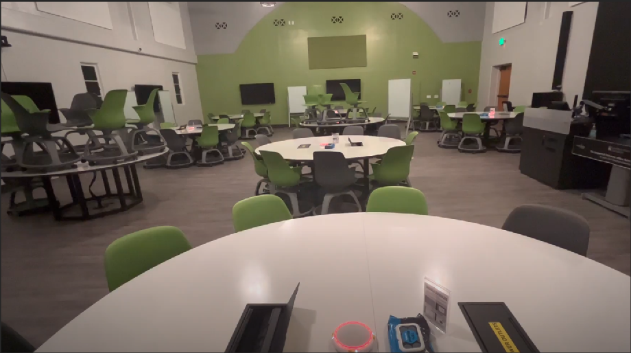
Figure 11: Picture of classroom used for live testing.

Fig. 12 represents the chaotic trajectories and coverage. The $dc$ is set at 90% to compensate for the inaccuracies of the generated map. The SLAM process generated non-existent free space in certain areas of the map as a result of sensor problems. This $dc$ was a compromise to ensure the coverage task could be completed. The parameters of the BCPP application were set as follows: (1) the lateral footprint was set to 5.0 m, (2) the maximum acceleration was set to 0.1 m/$s^{2}$ (the maximum acceleration of the Turtlebot2), and (3) the wall distance was set to 0.36 m to accommodate the size of the Turtlebot2. The CCPP application provides the robot the ability to maneuver around the sets of tables and chairs, as well as the various whiteboards spread in the map.

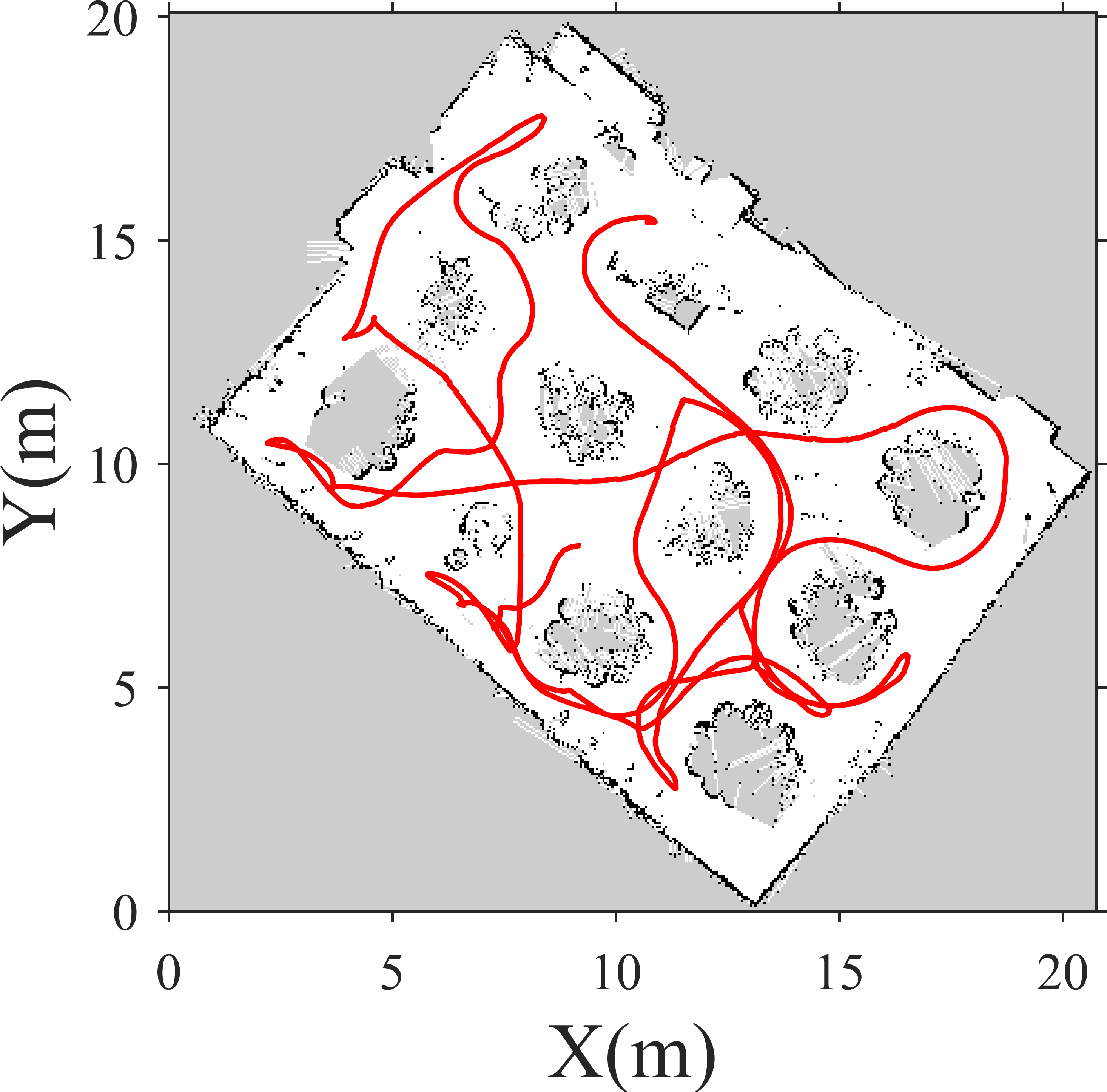
(a)

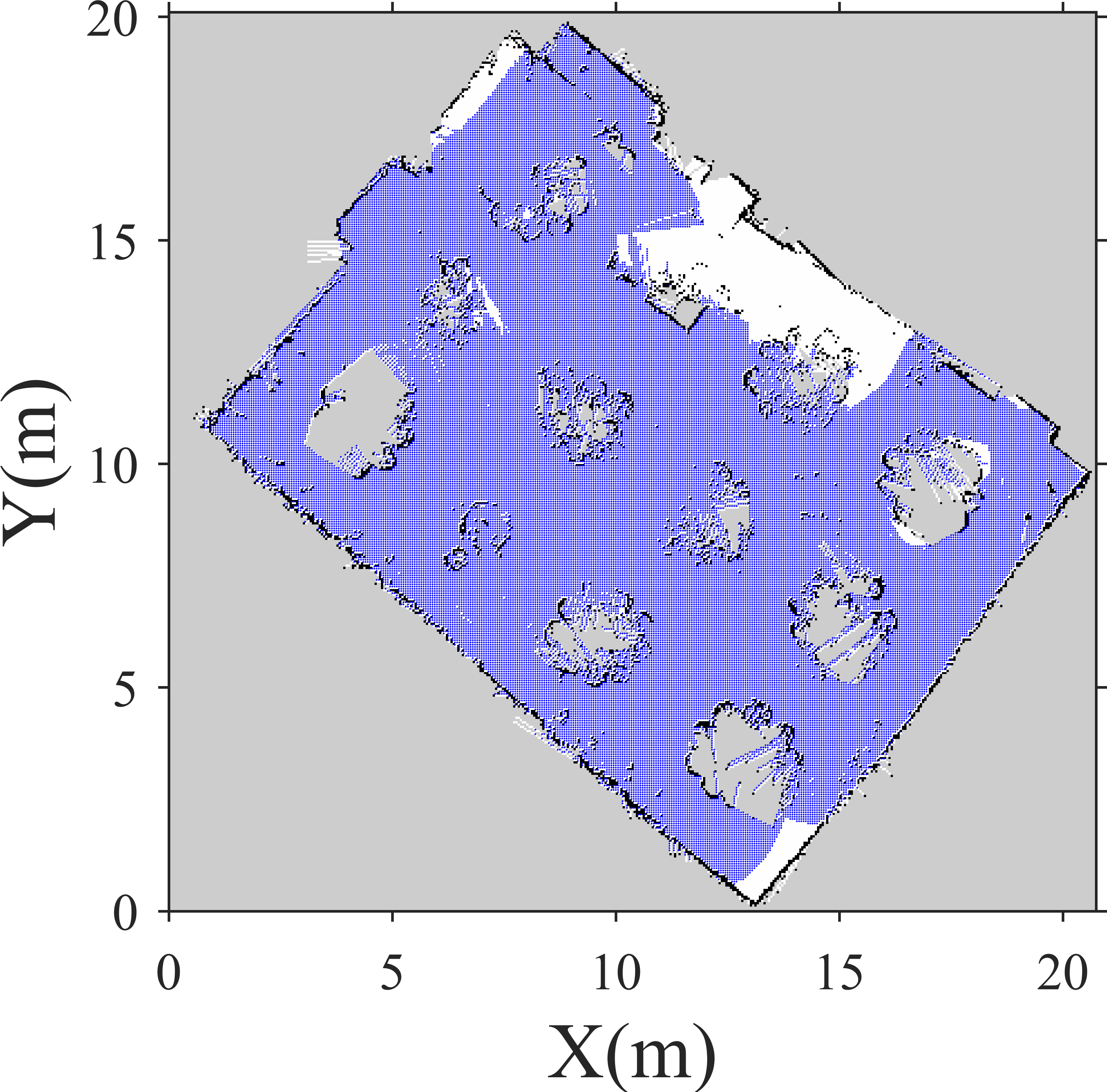
(b)

Figure 12: CCPP application ($SR$ = 2.5 m) used in a classroom for 90% coverage: (a) chaotic trajectories, and (b) covered cells.

Fig. 13 showcases the cellular decomposition and coverage plan of the classroom with the BCPP application ($CT$ at 10.42 minutes). As seen in Fig. 13, some of the obstacles (two sets of tables and chairs, and a white board) did not only have to be simplified, but combined into one polygon shape in order to ensure the cellular decomposition was computationally possible for the BCPP application to handle. Parts of the environment boundaries had to be simplified to this effect as well. It must be stated that a better CPU might have handled the necessary computations. A side by side view of the map in Fig.  13(a) (generated via SLAM) and the polygon representation of the environment in Figs.  13(b)-(c) show the critical differences in environment representation. The combination of sensor characteristics and inaccurate polygon representation of obstacles could cause significant coverage performance drop off within the context of thoroughness of coverage. It is possible that our CCPP method has the same advantages across all methods which use cellular decomposition, such as the Morse-based cellular decomposition method [Galceran and Carreras, 2013, Galceran and Carreras, 2012].

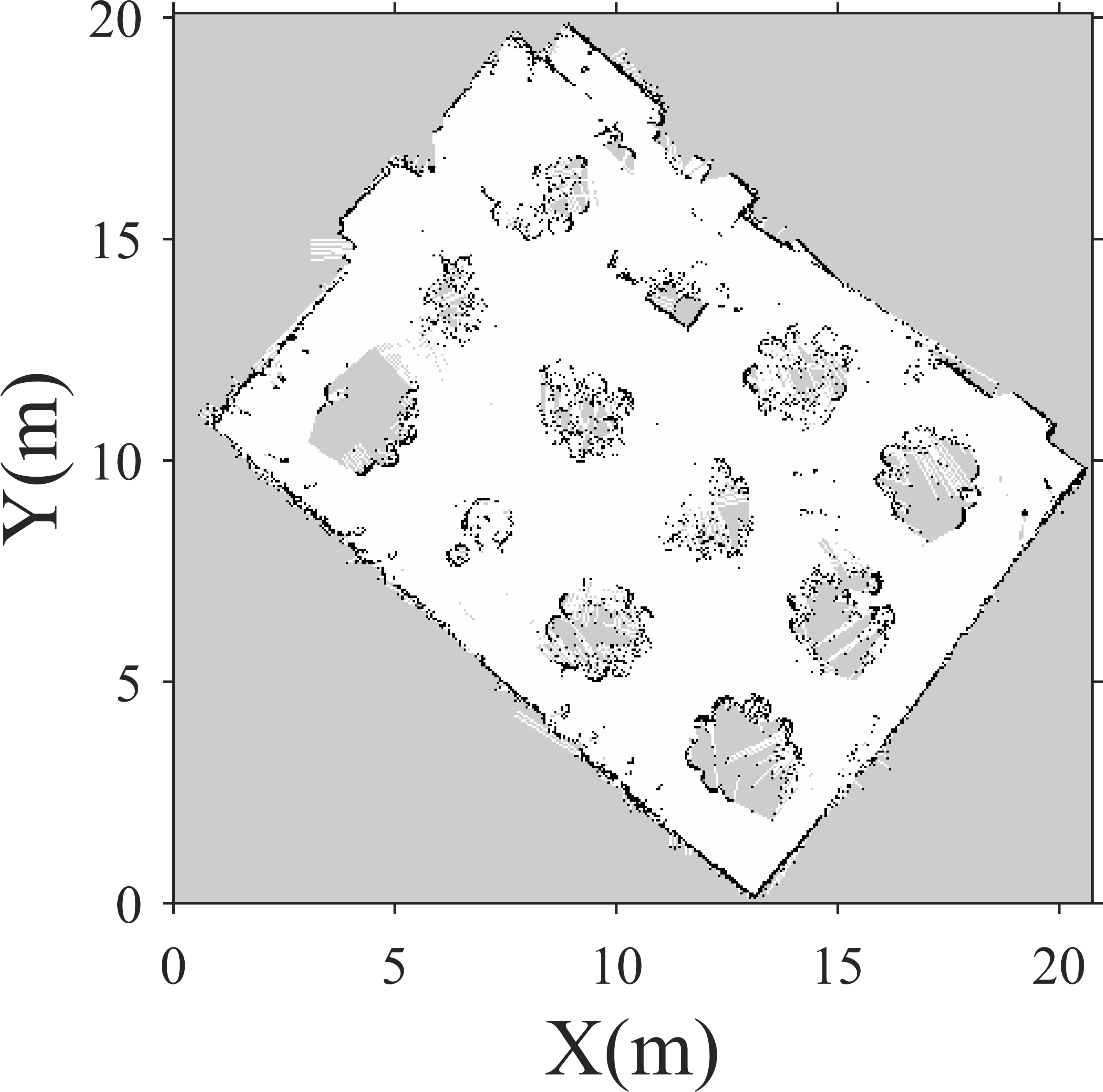
(a)

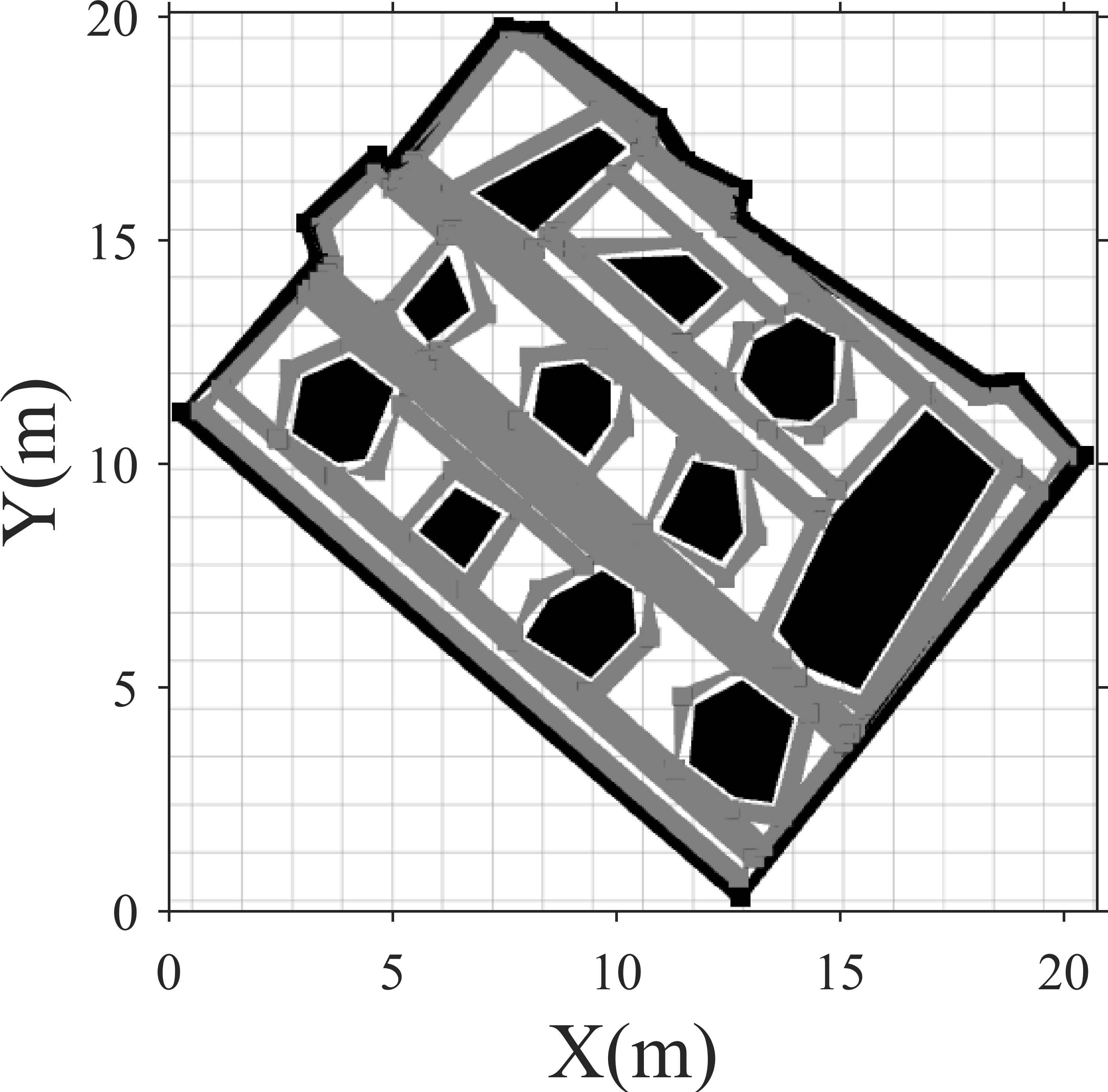
(b)

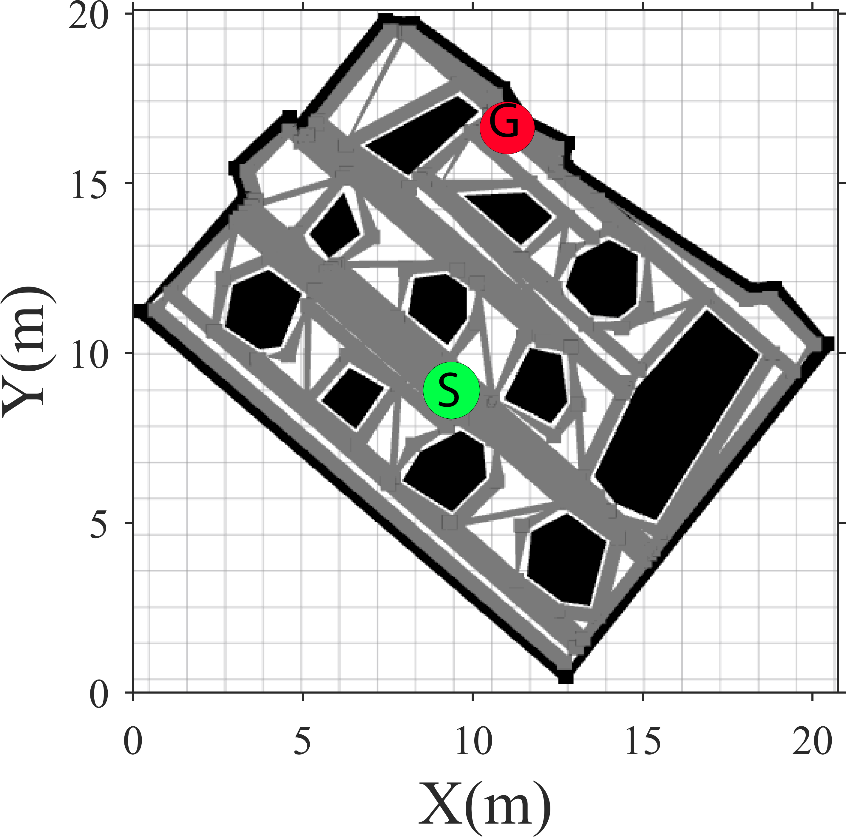
(c)

Figure 13: BCPP application ($LF$ = 5.0 m) used to cover classroom: (a) the map (generated via SLAM), (b) cellular decomposition, and (c) planned boustrophedon coverage path.

4.3 Test of computational speed of coverage calculation technique

This experiment was developed to test the computational performance of our coverage calculation method. The setup for this experiment is as follows. (1) The maximum velocity at which the simulated TurtleBot3 can reach is set to 5m/s. (2) The robot’s starting position is at one end of a runway (in simulation). The robot is driven in a straight line to the opposite end of the runway, which ends at a wall. (3) Upon the robot’s maximum velocity reaching 5m/s, the algorithms are signaled to start coverage calculation until the robot stops at the wall. (4) The distance traveled between each call of Algorithm 5 is recorded throughout the journey. Table  2 contains the maximum, minimum and average recorded distance of each experiment.

Table 2: Performance of computational speed of coverage calculation.

Runway	no. of Threads	$v$ (m/s)	$SR$ (m)	Average distance (m)	Max distance (m)	Min distance (m)
Runway 1	1	5.0	5.0	2.29	3.16	1.84
Runway 2	1	5.0	7.5	17.76	20.45	15.45
Runway 2	20	5.0	7.5	13.18	20.99	1.83
Runway 2	1	3.0	7.5	6.08	12.00	2.15

These recorded distances provide the basis for judging the computational efficiency of coverage calculation. If the average recorded distance is less than the $SR$, this means that coverage updates generally occur at a faster rate than the robot is able to completely move out of the area covered during the previous iteration of Algorithm 4. For this experiment, the sensor $FOV$ is set from 0 to 6.28 radians, and sensor $FOV$ mapping is configured so that the coverage status of every queried cell is updated. In this way, accurate coverage is neglected for the sake of maximizing the computational burden placed on our coverage calculation method. For this experiment, Algorithm 4 includes a multi-threading option that divides the cells $\in$ Query into subsets, which are then processed with separate threads of Algorithm 5 for possibly faster computation. Multi-threading is tested to check for any improvements in computational performance. It must be noted that: (1) the value of 1 in the ”no. of threads” column of Table  2 represents no multi-threading, and (2) the maximum velocity value of 5m/s was chosen as this was the highest robot velocity that the simulation would allow without creating computational errors within the physics engine of Gazebo.

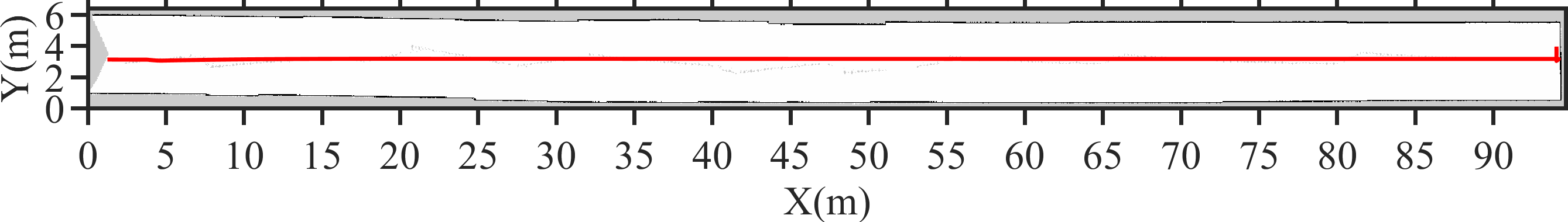
(a)

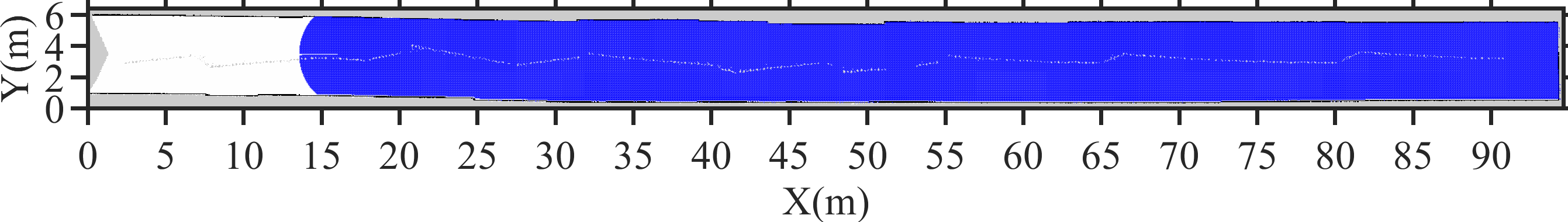
(b)

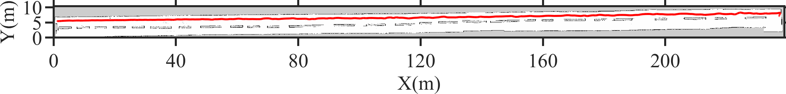
(c)

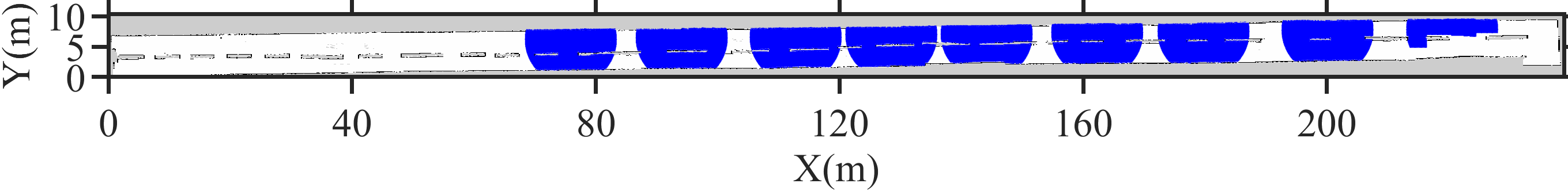
(d)

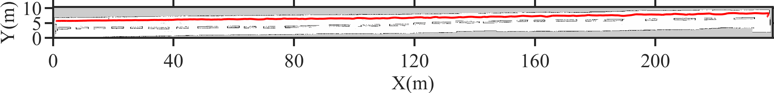
(e)

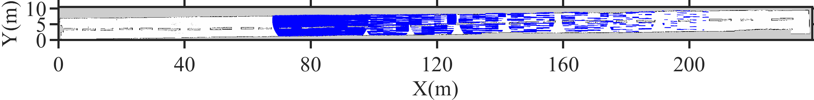
(f)

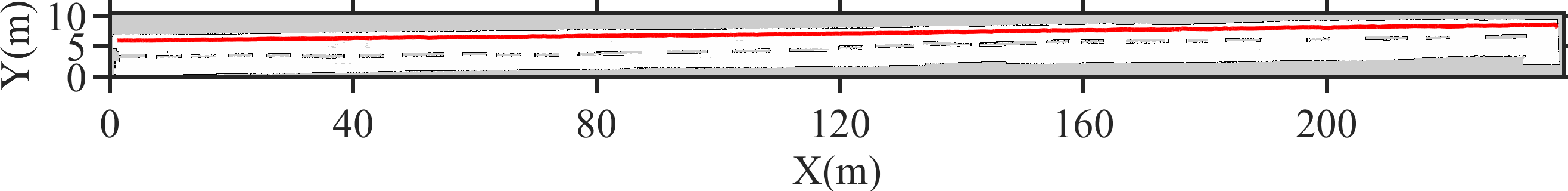
(g)

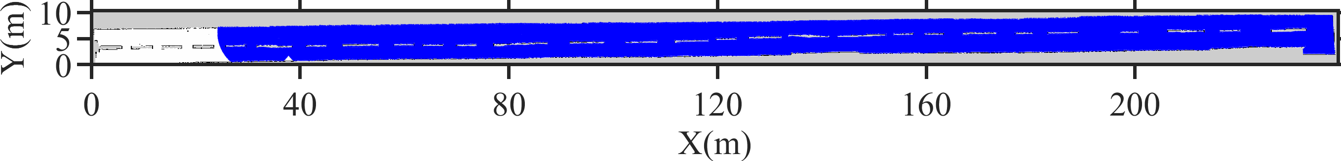
(h)

Figure 14: The visual representation of the performance of the coverage calculation method tested on 2 simulated runways. The figures on the left and right depict the robot’s trajectory and coverage across the runway, respectively. (a, b) Runway 1, No. of Threads$=1$, $v=5$ m/s, $SR=5$ m; (c, d) Runway 2, No. of Threads$=1$, $v=5$ m/s, $SR=7.5$ m ; (e, f) Runway 2, No. of Threads$=20$, $v=5$ m/s, $SR=7.5$ m ; (g, h) Runway 2, No. of Threads$=1$, $v=3$ m/s, $SR=7.5$ m.

Figs. 14(a),(c),(e) and (g) depict the straight line trajectory of robot from one end of a runway to the other. Fig. 14(b),(d),(f) and (h) depict the coverage started from the point at which simulated Turtlebot3 reaches the maximum velocity on the aforementioned trajectory. The smallest runway (Figs. 14(a) and (b)) is covered using an $SR$ of 5.0 m. The average, maximum and minimum recorded distances are 2.29 m, 3.16 m, and 1.84 m, respectively. This means that at no point is there a gap in coverage update. That is to say, from the first to the last call of Algorithm 5, the entire area within that time frame is covered (as seen in Fig. 14(b)). The biggest runway (Figs. 14(c) to (h)) is covered using an $SR$ of 7.5 m. As an aside, the obstacles placed in the middle of the runway provided unique features which enabled mapping the runway environment. With multi-threading disabled, the average, maximum and minimum recorded distances are 17.76 m, 20.45 m, 15.45 m, respectively. These values indicate that there will be gaps in the coverage, and Fig. 14(d) visually shows this result. With multi-threading (20 threads) the average, maximum and minimum recorded distances are 13.18 m, 20.99 m, 1.83 m, respectively. The average distance is incongruent with what is shown in Fig. 14(f). We speculate that the Python Global Interpreter Lock (GIL) and the Operating System Thread Scheduler delay the execution of threads across the iterations of Algorithm 4. Therefore, threads from previous iterations could still be in queue to start or finish their execution. This results in the peculiar breaks in coverage shown in Fig. 14(f). Developing the source code in programming languages (such as C++) that are not limited by the GIL could possibly solve this issue and lead to effective use of the multi-threading option for faster computations of the coverage.

As a last trial run, we reduced the speed of the maximum velocity of the Turtlebot3 to 3 m/s and ran the same experiment with multi-threading disabled at this velocity. The average, maximum and minimum distances are 6.08 m, 12.00 m and 2.15 m respectively (see Figs. 14 (g) and (h)). This shows that all areas between the start and end of coverage calculations are completely covered. The computation speed of coverage calculation enables effective coverage rate update even at robot speeds of up to 3 m/s with $SR$ at 7.5 m.

4.4 Parameters influence on coverage time

This section discusses the effect of parameters on coverage time. Two environments have been covered multiple times using different sets of parameters, and the resulting coverage times have been recorded in Table  3. Fig. 15 depicts the maps of these environments. The names of the environments shown in Figs. 15(a)-(b) are: (1) Bungalow, and (2) LDW1 in that order. The $dc$ for every experiment was set to 90%. The robot’s starting position was kept the same for every test carried out in an environment, and the velocity ($v$) for every experiment was 0.22m/s. The simulated Turtlebot3 and 2D LiDAR were utilized in all experiments. The $FOV$ for all experiments is ranging from 0 to 6.28 radians. The maximum sensing area for all experiments is 38.48 $m^{2}$. From the results in Table 3, we try to glean some general patterns in coverage performance within the context of $CT$.

Table 3: Performance of CCPP on two environments under various parameters.

Map	Approximate free area ($m^{2}$)	Case #	Maximum Sensing Area ($m^{2}$)	$n_{iter}$	$ns$	no. of zones	Average Zone Size ($m^{2}$)	$CT$ (min)	ratio
Bungalow	365.03	1	38.48	1000	20	15	24.34	38.12	1.58
		2		10	10	15		9.01
		3		1000	20	50	7.30	65.72	5.27
		4		10	10	50		13.50
		5		10	10	25	14.60	12.06	2.64
LDW1	1146.34	6	38.48	20	20	25	45.85	30.43	0.84
		7		2000	20	15	76.42	92.14	0.50
		8		20	20	50	22.93	31.01	1.68
		9		2000	20	50		179.68
Esquare	1010.44	10	38.48	20	20	21	48.12	24.88	0.80
		11		1000	20	21		57.57
		12		20	20	45	22.45	24.47	1.71
		13		1000	20	45		61.44

Due to the fact that parameters must be set manually, we discovered the following. (1) Setting the number of zones such that the ratio of the maximum sensing area to the average zone size greater or equal to one is more favorable, as $n_{iter}$ does not need to be set high to reach $dc$. In this way, there is less burden in making some kind of educated guess as to how high to set $n_{iter}$ to even reach $dc$ much less perform the coverage task within a reasonable time frame. (2) In the same vain, setting the number of zones such that the ratio of the maximum sensing area to the average zone size is less than one is less favorable. A wrong guess on the $n_{iter}$ value could at best, result in a $CT$ that deviates drastically from the optimal $CT$. At worst, the wrong $n_{iter}$ results in a scenario where $dc$ is never reached. However, (3) it is not necessary that the ratio is greater or equal to one. From cases 6 and 8, which have a ratio of 0.84 and 1.68 respectively, the $CT$ was approximately the same (about 30 minutes at $n_{iter}=$20) as well as the lowest for LDW1. It could be the case that a ratio$\approx$1 is good enough. (4) From cases 2, 4, 5 (see Table 3), we found that at low $n_{iter}$, a further increase in ratio beyond an approximate value of 2 may not result in better $CT$. For Bungalow, a ratio of 1.58, 5.27, and 2.64 result in a $CT$ of 9.01, 13.50 and 12.06 minutes respectively (at $n_{iter}=$10). (5) From cases 1 and 3, we found that for a high $n_{iter}$, a further increase in ratio beyond an approximate value of 2 may not result in better $CT$. (6) From cases 7 and 9, we found that a ratio much less than 1 (0.5) with a high enough $n_{iter}$ could result in lower $CT$ than a run with a ratio$\geq$1. This finding is not particularly relevant, as cases 7 and 9 had the longest coverage times in LDW1.

Ultimately, it is uncertain as to whether the findings (3) to (6) are general patterns. There could be a great deal of interplay between the results and the environment properties (size, shape, obstacle density e.t.c). We made sure to corroborate these findings using a simple environment, Esquare. Cases 10 and 12 seem to support finding (3) and (4), especially (3). Cases 11 and 13 seem to support cases (5) and (6). However, it is important to reinstate that the properties of the results (and the properties of the robot) could play a huge role in the results.

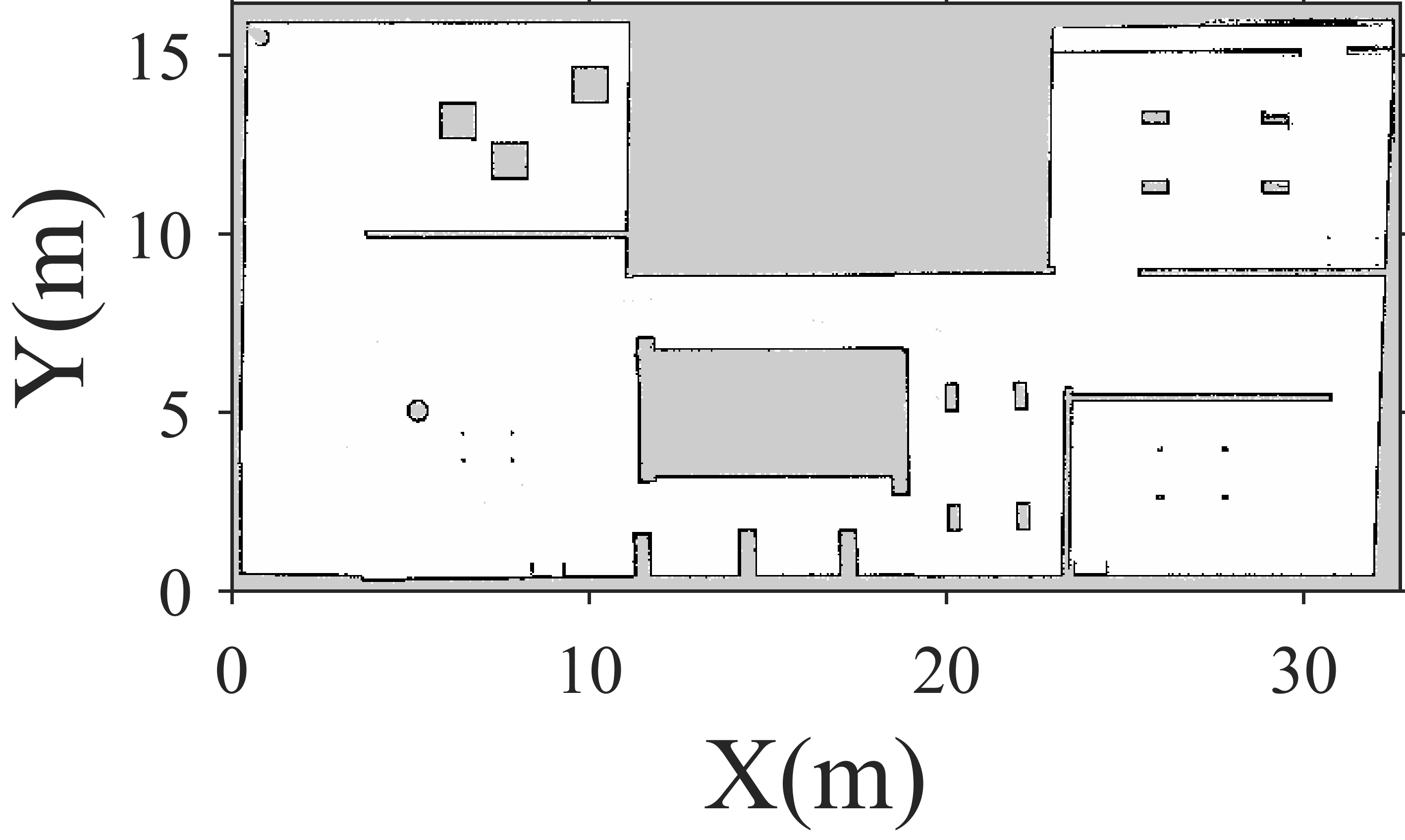
(a)

(b)

Figure 15: Maps of simulated environments: (a) Bungalow, and (b) LDW1.

5 Conclusions

This study proposes new techniques to realize the application of CCPP in realistic environments. Three techniques were developed to achieve this goal. These contributions were integrated to develop a new CCPP application in the ROS framework that enables effective coverage of large, complex-shaped environments with varying obstacle densities. The developed coverage calculation technique was shown to be computationally efficient at speeds up to 5 m/s for a robot with sensing range of 5.0 m. A multi-threading option could possibly provide faster computation for coverage calculations if the source code is developed in a programming language like C++ which is not limited by a global interpreter lock. Due to use of occupancy-grid maps, our method is susceptible to exponential memory usage dependent on size of environment and resolution used for grid map representation. This could lead to memory errors. Further work must be done to tackle this issue. The performance of our CCPP application was tested against a more established CPP, the boustrophedon coverage path planner. The BCPP application used for this comparison performed coverage at shorter coverage times, but the CCPP was shown to have the potential to match it in certain environments if provided with the right set of system parameters. At the same time, the CCPP provides the unpredictability in the motion necessary to avoid attacks in adversarial environments. These findings must however be verified with extensive testing using a BCPP application which provides a robot in realistic simulation environments such as Gazebo or real-life environments to allow recording realistic coverage times. Further research is required to develop a machine-learning technique that enables CCPP to autonomously determine a proper combination of parameter values that would provide optimized coverage based on the robot’s properties and the known properties of the covered environment. The CCPP method was shown to have potential advantages over BCPP due to the computational complexity involved in cellular decomposition. It is therefore plausible that our CCPP method has these same advantages over all methods which use cellular decomposition, for instance, the Morse-based cellular decomposition method. Future study should involve the testing of the CCPP method against other types of CPP methods. Lastly, the development of a local planner specifically for use in CCPP will help to improve the efficiency of the planner.

References

- Agiza and Yassen, 2001 Agiza, H. and Yassen, M. (2001). Synchronization of rossler and chen chaotic dynamical systems using active control. Physics Letters A, 278(4):191–197.
- Arrowsmith et al., 1993 Arrowsmith, D. K., Cartwright, J. H., Lansbury, A. N., and Place, C. M. (1993). The bogdanov map: Bifurcations, mode locking, and chaos in a dissipative system. International Journal of Bifurcation and Chaos, 3(04):803–842.
- Bae, 2004a Bae, Y. (2004a). Obstacle avoidance method in the chaotic robot. In The 23rd Digital Avionics Systems Conference (IEEE Cat. No. 04CH37576), volume 2, pages 12–D. IEEE.
- Bae, 2004b Bae, Y. (2004b). Target searching method in the chaotic mobile robot. In The 23rd Digital Avionics Systems Conference (IEEE Cat. No. 04CH37576), volume 2, pages 12–D. IEEE.
- Bae et al., 2006 Bae, Y., Lee, M., and Gatton, T. M. (2006). An obstacle avoidence method for chaotic robots using angular degree limitions. In International Conference on Computational Science and Its Applications, pages 244–250. Springer.
- Bae et al., 2003 Bae, Y.-C., Kim, J.-W., and Kim, Y.-G. (2003). Obstacle avoidance methods in the chaotic mobile robot with integrated some chaos equation. International Journal of Fuzzy Logic and Intelligent Systems, 3(2):206–214.
- Bähnemann et al., 2021 Bähnemann, R., Lawrance, N., Chung, J. J., Pantic, M., Siegwart, R., and Nieto, J. (2021). Revisiting boustrophedon coverage path planning as a generalized traveling salesman problem. In Field and Service Robotics: Results of the 12th International Conference, pages 277–290. Springer.
- Bormann et al., 2018 Bormann, R., Jordan, F., Hampp, J., and Hägele, M. (2018). Indoor coverage path planning: Survey, implementation, analysis. In 2018 IEEE International Conference on Robotics and Automation (ICRA), pages 1718–1725. IEEE.
- Choi et al., 2017 Choi, S., Lee, S., Viet, H. H., and Chung, T. (2017). B-theta*: an efficient online coverage algorithm for autonomous cleaning robots. Journal of Intelligent & Robotic Systems, 87(2):265–290.
- Choi et al., 2020 Choi, Y., Choi, Y., Briceno, S., and Mavris, D. N. (2020). Energy-constrained multi-uav coverage path planning for an aerial imagery mission using column generation. Journal of Intelligent & Robotic Systems, 97(1):125–139.
- Choset, 2000 Choset, H. (2000). Coverage of known spaces: The boustrophedon cellular decomposition. Autonomous Robots, 9:247–253.
- Choset and Pignon, 1998 Choset, H. and Pignon, P. (1998). Coverage path planning: The boustrophedon cellular decomposition. In Field and service robotics, pages 203–209. Springer.
- Chu et al., 2022 Chu, H., Yi, J., and Yang, F. (2022). Chaos particle swarm optimization enhancement algorithm for uav safe path planning. Applied Sciences, 12(18):8977.
- Coombes et al., 2019 Coombes, M., Chen, W.-H., and Liu, C. (2019). Flight testing boustrophedon coverage path planning for fixed wing uavs in wind. In 2019 International Conference on Robotics and Automation (ICRA), pages 711–717. IEEE.
- Curiac and Volosencu, 2014 Curiac, D.-I. and Volosencu, C. (2014). A 2d chaotic path planning for mobile robots accomplishing boundary surveillance missions in adversarial conditions. Communications in Nonlinear Science and Numerical Simulation, 19(10):3617–3627.
- Di Franco and Buttazzo, 2016 Di Franco, C. and Buttazzo, G. (2016). Coverage path planning for uavs photogrammetry with energy and resolution constraints. Journal of Intelligent & Robotic Systems, 83(3):445–462.
- ethz-asl / polygon_coverage_planning github, 2023 ethz-asl / polygon_coverage_planning github (2023). https://github.com/ethz-asl/polygon_coverage_planning.
- Faigl et al., 2011 Faigl, J., Kulich, M., and Přeučil, L. (2011). A sensor placement algorithm for a mobile robot inspection planning. Journal of Intelligent & Robotic Systems, 62(3):329–353.
- Fallahi and Leung, 2010 Fallahi, K. and Leung, H. (2010). A cooperative mobile robot task assignment and coverage planning based on chaos synchronization. International Journal of Bifurcation and Chaos, 20(01):161–176.
- Galceran and Carreras, 2012 Galceran, E. and Carreras, M. (2012). Efficient seabed coverage path planning for asvs and auvs. In 2012 IEEE/RSJ International Conference on Intelligent Robots and Systems, pages 88–93. IEEE.
- Galceran and Carreras, 2013 Galceran, E. and Carreras, M. (2013). A survey on coverage path planning for robotics. Robotics and Autonomous systems, 61(12):1258–1276.
- Gomez et al., 2017 Gomez, J. I. V., Melchor, M. M., and Lozada, J. C. H. (2017). Optimal coverage path planning based on the rotating calipers algorithm. In 2017 International Conference on Mechatronics, Electronics and Automotive Engineering (ICMEAE), pages 140–144. IEEE.
- Gonzalez et al., 2005 Gonzalez, E., Alvarez, O., Diaz, Y., Parra, C., and Bustacara, C. (2005). Bsa: A complete coverage algorithm. In proceedings of the 2005 IEEE international conference on robotics and automation, pages 2040–2044. IEEE.
- Greenzie / boustrophedon_planner github, 2023 Greenzie / boustrophedon_planner github (2023). https://github.com/Greenzie/boustrophedon_planner.
- Grøtli and Johansen, 2012 Grøtli, E. I. and Johansen, T. A. (2012). Path planning for uavs under communication constraints using splat! and milp. Journal of Intelligent & Robotic Systems, 65(1):265–282.
- Hameed, 2014 Hameed, I. A. (2014). Intelligent coverage path planning for agricultural robots and autonomous machines on three-dimensional terrain. Journal of Intelligent & Robotic Systems, 74(3):965–983.
- Hsu et al., 2014 Hsu, P.-M., Lin, C.-L., and Yang, M.-Y. (2014). On the complete coverage path planning for mobile robots. Journal of Intelligent & Robotic Systems, 74(3):945–963.
- Huang et al., 2020 Huang, X., Sun, M., Zhou, H., and Liu, S. (2020). A multi-robot coverage path planning algorithm for the environment with multiple land cover types. IEEE Access, 8:198101–198117.
- Ipiano / coverage-planner github, 2023 Ipiano / coverage-planner github (2023). https://github.com/Ipiano/coverage-planning.
- Jan et al., 2019 Jan, G. E., Luo, C., Lin, H.-T., and Fung, K. (2019). Complete area coverage path-planning with arbitrary shape obstacles. Journal of Automation and Control Engineering Vol, 7(2).
- Jansri et al., 2004 Jansri, A., Klomkarn, K., and Sooraksa, P. (2004). On comparison of attractors for chaotic mobile robots. In 30th Annual Conference of IEEE Industrial Electronics Society, 2004. IECON 2004, volume 3, pages 2536–2541. IEEE.
- Kapoutsis et al., 2017 Kapoutsis, A. C., Chatzichristofis, S. A., and Kosmatopoulos, E. B. (2017). Darp: divide areas algorithm for optimal multi-robot coverage path planning. Journal of Intelligent & Robotic Systems, 86(3):663–680.
- Li et al., 2015 Li, C., Song, Y., Wang, F., Liang, Z., and Zhu, B. (2015). Chaotic path planner of autonomous mobile robots based on the standard map for surveillance missions. Mathematical Problems in Engineering, 2015.
- Li et al., 2016 Li, C., Song, Y., Wang, F., Wang, Z., and Li, Y. (2016). A bounded strategy of the mobile robot coverage path planning based on lorenz chaotic system. International journal of advanced robotic systems, 13(3):107.
- Li et al., 2013 Li, C., Wang, F., Zhao, L., Li, Y., and Song, Y. (2013). An improved chaotic motion path planner for autonomous mobile robots based on a logistic map. International Journal of Advanced Robotic Systems, 10(6):273.
- Li et al., 2017 Li, C.-h., Song, Y., Wang, F.-y., Wang, Z.-q., and Li, Y.-b. (2017). A chaotic coverage path planner for the mobile robot based on the chebyshev map for special missions. Frontiers of Information Technology & Electronic Engineering, 18(9):1305–1319.
- Li et al., 2014 Li, Y., Li, D., Maple, C., Yue, Y., and Oyekan, J. (2014). K-order surrounding roadmaps path planner for robot path planning. Journal of Intelligent & Robotic Systems, 75(3):493–516.
- Lü et al., 2004 Lü, J., Chen, G., and Cheng, D. (2004). A new chaotic system and beyond: the generalized lorenz-like system. International Journal of Bifurcation and Chaos, 14(05):1507–1537.
- Majeed, 2020 Majeed, A. I. (2020). Mobile robot motion control based on chaotic trajectory generation. Journal of Engineering and Sustainable Development, 24(4):48–55.
- Moysis et al., 2020a Moysis, L., Petavratzis, E., Marwan, M., Volos, C., Nistazakis, H., and Ahmad, S. (2020a). Analysis, synchronization, and robotic application of a modified hyperjerk chaotic system. Complexity, 2020.
- Moysis et al., 2020b Moysis, L., Petavratzis, E., Volos, C., Nistazakis, H., and Stouboulos, I. (2020b). A chaotic path planning generator based on logistic map and modulo tactics. Robotics and Autonomous Systems, 124:103377.
- Moysis et al., 2021 Moysis, L., Rajagopal, K., Tutueva, A. V., Volos, C., Teka, B., and Butusov, D. N. (2021). Chaotic path planning for 3d area coverage using a pseudo-random bit generator from a 1d chaotic map. Mathematics, 9(15):1821.
- Nakamura and Sekiguchi, 2001 Nakamura, Y. and Sekiguchi, A. (2001). The chaotic mobile robot. IEEE Transactions on Robotics and Automation, 17(6):898–904.
- Nasr et al., 2019 Nasr, S., Mekki, H., and Bouallegue, K. (2019). A multi-scroll chaotic system for a higher coverage path planning of a mobile robot using flatness controller. Chaos, Solitons & Fractals, 118:366–375.
- nav_msgs/Path.msg, 2023 nav_msgs/Path.msg (2023). http://docs.ros.org/en/api/nav_msgs/html/msg/Path.html.
- Ntawumenyikizaba et al., 2012 Ntawumenyikizaba, A., Viet, H. H., and Chung, T. (2012). An online complete coverage algorithm for cleaning robots based on boustrophedon motions and a* search. In 2012 8th International Conference on Information Science and Digital Content Technology (ICIDT2012), volume 2, pages 401–405. IEEE.
- Nwachioma and Pérez-Cruz, 2021 Nwachioma, C. and Pérez-Cruz, J. H. (2021). Analysis of a new chaotic system, electronic realization and use in navigation of differential drive mobile robot. Chaos, Solitons & Fractals, 144:110684.
- Petavratzis et al., 2020a Petavratzis, E., Moysis, L., Volos, C., Gupta, M. K., Stouboulos, I., and Goudos, S. (2020a). Chaotic motion control of a mobile robot using a memory technique. In 2020 24th International Conference on System Theory, Control and Computing (ICSTCC), pages 506–511. IEEE.
- Petavratzis et al., 2020b Petavratzis, E., Moysis, L., Volos, C., Nistazakis, H., Munoz-Pacheco, J. M., and Stouboulos, I. (2020b). Motion control of a mobile robot based on a chaotic iterative map. In 2020 9th International Conference on Modern Circuits and Systems Technologies (MOCAST), pages 1–4. IEEE.
- Petavratzis et al., 2020c Petavratzis, E., Moysis, L., Volos, C., Nistazakis, H., Stouboulos, I., et al. (2020c). Chaotic path planning for grid coverage using a modified logistic-may map. Journal of Automation, Mobile Robotics and Intelligent Systems, pages 3–9.
- Petavratzis et al., 2021a Petavratzis, E., Moysis, L., Volos, C., Stouboulos, I., Nistazakis, H., and Valavanis, K. (2021a). A chaotic path planning generator enhanced by a memory technique. Robotics and Autonomous Systems, 143:103826.
- Petavratzis et al., 2021b Petavratzis, E., Volos, C., Ouannas, A., Nistazakis, H., Valavanis, K., and Stouboulos, I. (2021b). A 2d discrete chaotic memristive map and its application in robot’s path planning. In 2021 10th International Conference on Modern Circuits and Systems Technologies (MOCAST), pages 1–4. IEEE.
- Pimentel-Romero et al., 2017 Pimentel-Romero, C., Muñoz-Pacheco, J. M., Felix-Beltran, O., Gomez-Pavon, L., and Volos, C. K. (2017). Chaotic planning paths generators by using performance surfaces. In Fractional Order Control and Synchronization of Chaotic Systems, pages 805–832. Springer.
- Quadtree implementation in Python, 2020 Quadtree implementation in Python (2020). https://scipython.com/blog/quadtrees-2-implementation-in-python.
- Rekleitis et al., 2008 Rekleitis, I., New, A. P., Rankin, E. S., and Choset, H. (2008). Efficient boustrophedon multi-robot coverage: an algorithmic approach. Annals of Mathematics and Artificial Intelligence, 52:109–142.
- Rjjxp/coverageplanning github, 2023 Rjjxp/coverageplanning github (2023). https://github.com/RJJxp/CoveragePlanning.
- Samet, 1988 Samet, H. (1988). An overview of quadtrees, octrees, and related hierarchical data structures. Theoretical Foundations of Computer Graphics and CAD, pages 51–68.
- sensor_msgs/LaserScan.msg, 2023 sensor_msgs/LaserScan.msg (2023). http://docs.ros.org/en/melodic/api/sensor_msgs/html/msg/LaserScan.html.
- Sooraska and Klomkarn, 2010 Sooraska, P. and Klomkarn, K. (2010). ” no-cpu” chaotic robots: from classroom to commerce. IEEE circuits and systems magazine, 10(1):46–53.
- Sridharan and Ahmadabadi, 2020 Sridharan, K. and Ahmadabadi, Z. N. (2020). A multi-system chaotic path planner for fast and unpredictable online coverage of terrains. IEEE Robotics and Automation Letters, 5(4):5268–5275.
- Sridharan et al., 2022 Sridharan, K., McNamee, P., Nili Ahmadabadi, Z., and Hudack, J. (2022). Online search of unknown terrains using a dynamical system-based path planning approach. Journal of Intelligent & Robotic Systems, 106(1):1–19.
- Tlelo-Cuautle et al., 2014 Tlelo-Cuautle, E., Ramos-López, H. C., Sánchez-Sánchez, M., Pano-Azucena, A. D., Sánchez-Gaspariano, L. A., Núñez-Pérez, J. C., and Camas-Anzueto, J. L. (2014). Application of a chaotic oscillator in an autonomous mobile robot. Journal of Electrical Engineering, 65(3):157.
- Volos et al., 2012a Volos, C. K., Bardis, N., Kyprianidis, I. M., and Stouboulos, I. N. (2012a). Implementation of mobile robot by using double-scroll chaotic attractors. Recent Researches in Applications of Electrical and Computer Engineering, pages 119–124.
- Volos et al., 2012b Volos, C. K., Kyprianidis, I. M., and Stouboulos, I. N. (2012b). A chaotic path planning generator for autonomous mobile robots. Robotics and Autonomous Systems, 60(4):651–656.
- Volos et al., 2013 Volos, C. K., Kyprianidis, I. M., and Stouboulos, I. N. (2013). Experimental investigation on coverage performance of a chaotic autonomous mobile robot. Robotics and Autonomous Systems, 61(12):1314–1322.
- Zhang, 2018 Zhang, C. (2018). Path planning for robot based on chaotic artificial potential field method. In IOP Conference Series: Materials Science and Engineering, volume 317, page 012056. IOP Publishing.
- Zhu et al., 2019 Zhu, D., Tian, C., Sun, B., and Luo, C. (2019). Complete coverage path planning of autonomous underwater vehicle based on gbnn algorithm. Journal of Intelligent & Robotic Systems, 94(1):237–249.