Statistical inference for counting processes under shape heterogeneity

Abstract

Proportional rate models are among the most popular methods for analyzing the rate function of counting processes. Although providing a straightforward rate-ratio interpretation of covariate effects, the proportional rate assumption implies that covariates do not modify the shape of the rate function. When such an assumption does not hold, we propose describing the relationship between the rate function and covariates through two indices: the shape index and the size index. The shape index allows the covariates to flexibly affect the shape of the rate function, and the size index retains the interpretability of covariate effects on the magnitude of the rate function. To overcome the challenges in simultaneously estimating the two sets of parameters, we propose a conditional pseudolikelihood approach to eliminate the size parameters in shape estimation and an event count projection approach for size estimation. The proposed estimators are asymptotically normal with a root-$n$ convergence rate. Simulation studies and an analysis of recurrent hospitalizations using SEER-Medicare data are conducted to illustrate the proposed methods.

1 Introduction

Statistical inferences of counting processes are often formulated based on their rate functions. The rate function is defined as the occurrence rate unconditional on the event history (Lawless and Nadeau, 1995; Lin et al., 2000), which is in contrast with the intensity function, defined as the occurrence rate conditional on history (Gail et al., 1980; Prentice et al., 1981; Andersen and Gill, 1982). The rate function has been commonly used for evaluating treatment effects or identifying risk factors. Denote by $\widetilde{N}(t)$ the number of events occurring at or before time $t$ and by $\bm Z$ a $p$-dimensional vector of covariates. Let $\mu(t\mid\bm Z)$ be the conditional rate function of $\widetilde{N}(\cdot)$ given $\bm Z$, that is, $\mu(t\mid\bm Z)dt=\operatorname{E}\{d\widetilde{N}(t)\mid\bm Z\}$. In the literature, various models have been proposed to describe the effect of $\bm Z$ on the rate function $\mu(t\mid\bm Z)$; popular choices include multiplicative models (Pepe and Cai, 1993; Lawless and Nadeau, 1995; Lin et al., 2000; Wang et al., 2001), additive models (Schaubel et al., 2006), scale-change models (Lin et al., 1998; Ghosh, 2004; Xu et al., 2017), and transformation models (Lin et al., 2001). The availability of these models allows investigators to identify an appropriate tool to conduct inference for each specific application but requires the model to be specified a priori. Since the rate function is a curve that depends on time and is intrinsically infinite-dimensional, correctly specifying the form of $\mu(t\mid\bm Z)$ can be challenging. Although graphical techniques and hypothesis testing have been commonly used for model checking, clear guidance on model selection and post-selection inference procedures are lacking. To avoid misleading conclusions drawn from misspecified models, one possible solution is to consider flexible models. On the other hand, models allowing full flexibility are often less favorable due to limited interpretability.

The goal of this paper is to develop a unified framework for modeling the rate function, which strikes a balance between flexibility and interpretability. Our framework is based on a decomposition of the rate function (Wang and Huang, 2014). Let $[0,\tau]$ be the time period of interest. Following Wang and Huang (2014), one can express the rate function as the product of a size component and a shape component: the size, defined as $\operatorname{E}\{\widetilde{N}(\tau)\mid\bm Z\}=\int_{0}^{\tau}\mu(t\mid\bm Z)dt$, is the expected number of events over the entire study period; the shape, defined as $\mu(t\mid\bm Z)/\operatorname{E}\{\widetilde{N}(\tau)\mid\bm Z\}$, characterizes the time-varying profile of the event rate standardized by its magnitude. The shape-size decomposition of the aforementioned rate-based models is presented in Figure 1. The figure demonstrates that shape is covariate-independent under the multiplicative model, while it depends on covariates in different ways under other models. Additionally, it is noted that existing approaches generally assume that size is monotonically increasing in a linear combination of covariates, allowing us to interpret the association between covariates and the total event count.

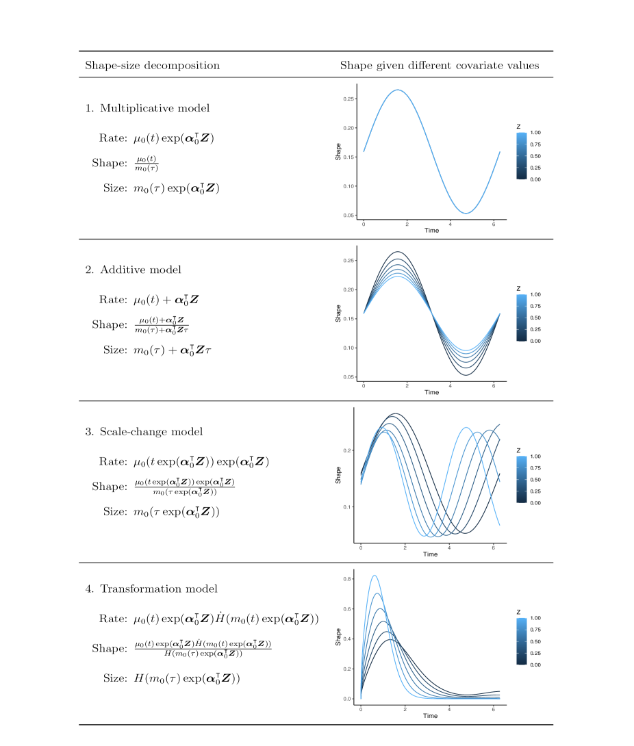
Figure 1: Shape and size decomposition of common recurrent event models. $\bm\alpha_{0}$ is a vector of regression parameters; $\mu_{0}(t)$ and $m_{0}(t)=\int_{0}^{t}\mu_{0}(u)du$ are the baseline rate and cumulative rate functions, respectively. For the transformation model, $H$ is an increasing function, and $\dot{H}$ is its first order derivative. The right column shows how covariates affect the shape function under a special case where $\bm Z$ is one dimensional, $\mu_{0}(t)=\sin(t)+1.5$, $\alpha_{0}=1$, and $H$ is the cumulative distribution function of the Weibull distribution with shape parameter 1.5 and scale parameter 5.

In this paper, we focus on the case of shape heterogeneity, where the shape of the rate function varies based on covariates. In our motivating SEER-Medicare data example (Warren et al., 2002; Enewold et al., 2020), the events of interest are repeated inpatient hospitalizations after the diagnosis of breast cancer. Younger patients tend to recover more quickly, and their hospitalizations are more likely to occur in the early phase after diagnosis. Older patients, on the other hand, have a more consistent rate of hospitalization over time. This implies that the shape of the hospitalization rate may depend on age at diagnosis, and the heterogeneity in shape should be taken into account when modeling the rate function. In this case, one may wonder how to draw definitive conclusions, such as whether a larger covariate is associated with an increased risk of events. To solve this problem, we propose a shape-size model. The model indexes the shape of the rate function using a linear predictor, which captures the relationship between the shape and multiple covariates; the size of the rate function is modeled through a separate index. Our model extends the original single index model (see, for example, Powell et al., 1989; Härdle and Stoker, 1989; Härdle et al., 1993; Ichimura, 1993) for a scalar outcome to a counting process outcome and offers a reasonable compromise between parametric and fully nonparametric modeling.

Single index models for the time to a single event under censoring have been widely studied in the literature. Researchers have considered proportional hazards regression where the hazard ratio depends on a single index (Huang and Liu, 2006; Wang et al., 2009). Without the proportional hazards assumption, single index models for the density function (Bouaziz and Lopez, 2010; Strzalkowska-Kominiak and Cao, 2013, 2014), the mean (Lopez, 2009; Lopez et al., 2013; Huang et al., 2020), the hazard function (Ding et al., 2013; Chiang et al., 2018), and the quantile function (Kong and Xia, 2017; Christou and Akritas, 2019; Bücher et al., 2021) of the event time have also been studied. However, single index models for the counting processes of recurrent events have been less studied. Zhao and Zhou (2014) considered sufficient dimension reduction for the rate of nonstationary Poisson processes and assumed that covariates do not modify the shape of the rate function. Bouaziz et al. (2015) considered a single index model where the rate function is indexed by a linear combination of covariates but did not distinguish the effects on shape and size.

The contribution of our work is twofold. First, we focus on the case where shape is covariate-dependent, and thus our method serves as a natural alternative when the commonly used proportional rate model (i.e., multiplicative model) does not hold. When assuming that size depends on covariates through an exponential link, we obtain comparable interpretations on the size component. Compared to other rate models where shape depends on covariates, our model is more flexible and allows covariates to have different effects on shape and size. Second, our model can involve up to two unspecified link functions, while existing single index models typically have one link function. To overcome the methodological challenges, we propose a two-step estimation procedure. In the first step, we estimate shape parameters through a conditional pseudolikelihood approach that eliminates size parameters. In the second step, we use the estimated shape function to project the event count from the follow-up period to the time interval of interest; regression analysis is then performed on the projected event count to estimate the size parameters.

This paper is organized as follows. In Section 2, we introduce the model setup. In Section 3, we propose a conditional pseudolikelihood approach to estimate the shape parameters; in addition, we propose a simplified estimator with a lower computational cost and the same asymptotic variance. In Section 4, we propose a unified approach for size estimation under different assumptions of link functions. In Section 5, we conduct simulation studies to evaluate the finite sample performance of the estimators. In Section 6, the proposed methods are applied to model the recurrent hospitalizations in SEER-Medicare breast cancer data. A discussion in Section 7 concludes the paper.

2 Model setup

We propose the following model for the conditional rate function,

$$\mu(t\mid\bm Z)=f(t,\bm\beta_{0}^{\intercal}\bm Z)g(\bm\gamma_{0}^{\intercal}\bm Z),~{}~{}0\leq t\leq\tau,$$ (1)

where $\bm\beta_{0}$ and $\bm\gamma_{0}$ are $p$-dimensional vectors of regression parameters, $f(t,\bm\beta_{0}^{\intercal}\bm Z)$ is the shape function indexed by $\bm\beta_{0}^{\intercal}\bm Z$, and $g(\cdot)$ is the size function indexed by $\bm\gamma_{0}^{\intercal}\bm Z$. We assume that the shape function $f(\cdot,x)$ is an unknown function satisfying $\int_{0}^{\tau}f(t,x)dt=1$ for any $x\in\mathbb{R}$. For identifiability, we assume that $\|\bm\beta_{0}\|=1$ and the $p$th element of $\bm\beta_{0}$ is positive, where $\|\cdot\|$ denotes the Euclidean norm. The size function $g(\cdot)$ can be either prespecified or unspecified.

In practice, the size parameter $\bm\gamma_{0}$ is the focus of interest and assumptions on $g(\cdot)$ can facilitate the interpretation of $\bm\gamma_{0}$. For example, when evaluating the effect of a risk factor, imposing monotonic assumptions on $g(\cdot)$ allows a better understanding of whether the factor is associated with a higher event risk. As another example, since we have $\operatorname{E}\{\widetilde{N}(\tau)\mid\bm Z\}=g(\bm\gamma_{0}^{\intercal}\bm Z)$, assuming $g(x)\propto\exp(x)$ yields a size ratio interpretation similar to a Poisson regression model for the total event count $\widetilde{N}(\tau)$. The interpretation of $\bm\beta_{0}$ is of less interest, and shape is estimated to ensure accurate estimation of the covariate effects on size. When assuming that $g(\cdot)$ is monotonically increasing, Models 2-4 in Figure 1 are special cases of Model (1) and force $\bm\beta_{0}/\bm\gamma_{0}$ to be a constant. In other words, Models 2-4 assume all the covariates have consistent effects on the shape and size. However, in real applications, such an assumption is often violated. We note that Sun et al. (2022) considered a more restricted shape-size model, where monotone constraints are imposed on the shape and size functions. However, monotone constraints on shape generally do not hold under the models in Figure 1 and are thus not imposed in our model. Additionally, to make interpretations more accessible to a broader audience, we incorporate a multiplicative size model as an extension of the proportional rate model; we also explored special cases where misspecified size models still yield consistent estimations of normalized covariate effects.

In practice, the process $\widetilde{N}(\cdot)$ may not be completely observed due to a limited follow-up period. Denote by $C=\min(C^{*},\tau)$ the censoring time, where $C^{*}$ is the time to the end of follow-up. We assume that $C$ is independent of $\widetilde{N}(\cdot)$ conditioning on $\bm Z$. The observed counting process is $N(t)=\widetilde{N}(\min(t,C))$, and we have $dN(t)=I(C\geq t)d\widetilde{N}(t)$. The observed data, denoted by $\{(N_{i}(t),\bm Z_{i},C_{i}),{t\in[0,\tau]},i=1,\ldots,n\}$, are assumed to be independent and identically distributed (i.i.d.) replicates of $\{(N(t),\bm Z,C),{t\in[0,\tau]}\}$.

3 Estimation of the shape parameters

3.1 Conditional likelihood under a working model

The estimation of shape parameters can be derived from a conditional pseudolikelihood approach that eliminates the size component $g(\bm\gamma_{0}^{\intercal}\bm Z)$. To motivate the estimation, we first consider a working assumption that $\widetilde{N}(\cdot)$ is a nonhomogeneous Poisson process. Later we will show that the estimator remains valid without the Poisson process assumption. Let $m_{i}=\widetilde{N}_{i}(C_{i})$ be the number of events observed on $[0,C_{i}]$. Conditional on $(C_{i},\bm Z_{i},m_{i})$, the event times, $T_{i1},\ldots,T_{im_{i}}$, are the order statistics of a set of i.i.d. random variables with the density function $f(t,\bm\beta_{0}^{\intercal}\bm Z_{i})/F(C_{i},\bm\beta_{0}^{\intercal}\bm Z_{i})$ (Cox and Lewis, 1966; Wang et al., 2001), where $F(t,x)=\int_{0}^{t}f(u,x)du$ is the cumulative shape function. The conditional likelihood of event times $(T_{i1},\ldots,T_{im_{i}})$ given $(C_{i},\bm Z_{i},m_{i})$, $i=1,\ldots,n$, is proportional to

$$\prod_{i=1}^{n}\prod_{k=1}^{m_{i}}\frac{f(T_{ik},\bm\beta^{\intercal}\bm Z_{i})}{F(C_{i},\bm\beta^{\intercal}\bm Z_{i})}.$$ (2)

Notably, the expression in (2) takes the form of likelihood for right-truncated data, where the truncation time for $T_{ik}$ is $C_{i}$. Define $r(t,x)=f(t,x)/F(t,x)$; then, we have $F(t,x)=\exp\{-\int_{t}^{\tau}r(u,x)du\}$. The log conditional likelihood, up to a constant, can be expressed as

$$\frac{1}{n}\sum_{i=1}^{n}\sum_{k=1}^{m_{i}}\left\{\log r(T_{ik},\bm\beta^{\intercal}\bm Z_{i})-\int_{T_{ik}}^{C_{i}}r(u,\bm\beta^{\intercal}\bm Z_{i})du\right\}.$$ (3)

To estimate $\bm\beta_{0}$, a natural idea is to “profile out” the nuisance function $r(t,x)$ in (3).

If $\bm\beta$ is known, we can construct a local conditional likelihood to estimate $r(t,x)$ and its integral. For each $x$, define $R(t,x)=\int_{t}^{\tau}r(u,x)du$, which is a decreasing function in $t$. We consider a discrete version of $R(\cdot,x)$, which is a left-continuous step function and jumps down at the observed event times. Specifically, let $R\{t,x\}$ be the decrease of $R(t,x)$ at $t$; then, the local log conditional likelihood can be written as

$$\sum_{i=1}^{n}\sum_{k=1}^{m_{i}}K_{h}(\bm\beta^{\intercal}\bm Z_{i}-x)\left(\log{R\{T_{ik},x\}}-\sum_{(j,l):T_{ik}\leq T_{jl}\leq C_{i}}R\{T_{jl},x\}\right),$$ (4)

where $K_{h}(\cdot)=K(\cdot/h)/h$ is a scaled kernel function, with $K(\cdot)$ being a kernel function with a bounded support on $[-1,1]$ and $h$ being a bandwidth parameter. In (4), subjects whose shape indices $\bm\beta^{\intercal}\bm Z$ are in a small neighborhood of $x$ are used to estimate $R(t,x)$. Elementary calculus shows that (4) is maximized by

$$\widehat{R}\{t,x\}=\frac{\sum_{i=1}^{n}\sum_{k=1}^{m_{i}}K_{h}(\bm\beta^{\intercal}\bm Z_{i}-x)I(T_{ik}=t)}{\sum_{i=1}^{n}\sum_{k=1}^{m_{i}}K_{h}(\bm\beta^{\intercal}\bm Z_{i}-x)I(T_{ik}\leq t\leq C_{i})}.$$

Given $N_{i}(t)=\sum_{k=1}^{m_{i}}I(T_{ik}\leq t)$, we construct the following estimator for $R(t,x)$,

$$\widehat{R}_{h}(t,x,{\bm\beta})=\int_{t}^{\tau}\frac{\sum_{i=1}^{n}K_{h}(x-{\bm\beta}^{\intercal}\bm Z_{i})dN_{i}(u)}{\sum_{i=1}^{n}K_{h}(x-{\bm\beta}^{\intercal}\bm Z_{i})N_{i}(u)I(C_{i}\geq u)}.$$ (5)

The log conditional likelihood (3) also involves $r(t,x)$, which can be estimated by the following bivariate kernel estimator,

$$\widehat{r}_{h}(t,x,{\bm\beta})=\frac{\sum_{i=1}^{n}\sum_{k=1}^{m_{i}}K_{h}(x-{\bm\beta}^{\intercal}\bm Z_{i})K_{h}(t-T_{ik})}{\sum_{i=1}^{n}K_{h}(x-{\bm\beta}^{\intercal}\bm Z_{i})N_{i}(t)I(C_{i}\geq t)}.$$

We plug $\widehat{r}_{h}$ and $\widehat{R}_{h}$ into (3) and obtain the following objective function:

$$\frac{1}{n}\sum_{i=1}^{n}\int_{0}^{\tau}\left\{\log\widehat{r}_{h}(t,\bm\beta^{\intercal}\bm Z_{i},\bm\beta)-\widehat{R}_{h}(t,\bm\beta^{\intercal}\bm Z_{i},\bm\beta)+\widehat{R}_{h}(C_{i},\bm\beta^{\intercal}\bm Z_{i},\bm\beta)\right\}dN_{i}(t).$$ (6)

Remark 3.1

Note that we replace $r(t,x)$ in (3) with $\widehat{r}_{h}(t,x)$ rather than the point mass $\widehat{R}\{t,x\}$. This is different from existing arguments of the profile likelihood for the Cox model, where the likelihood has a similar structure and the nuisance baseline hazard at event times is replaced by point masses (see, for example, Murphy and Van der Vaart, 2000). In our setting, replacing $r(t,x)$ in (3) with $\widehat{R}\{t,x\}$ does not yield a consistent estimator for $\bm\beta_{0}$. Moreover, for each $x$, $r(t,x)$ is mathematically equivalent to a reverse time hazard function, and our method can be easily adapted to estimate a single index hazard model for time to a single event. This is noteworthy because the existing local profile likelihood method has been shown to fail when applied to a single index hazard model (Ding et al., 2013).

Remark 3.2

The pseudo conditional likelihood approach can be applied when the form of the size function is misspecified, as the size function is eliminated in (2).

3.2 A simplified objective function

The objective function (6) can be further simplified to reduce the computational cost. Define $R(t,x,\bm\beta)=\int_{t}^{\tau}\operatorname{E}\{N(u)I(C\geq u)\mid\bm\beta^{\intercal}\bm Z=x\}^{-1}\operatorname{E}\{dN(u)\mid\bm\beta^{\intercal}\bm Z=x\}$ and we have $R(t,x,\bm\beta_{0})=R(t,x)$. The quantity $n^{-1}\sum_{i=1}^{n}\int_{0}^{\tau}\{\widehat{R}_{h}(t,\bm\beta^{\intercal}\bm Z_{i},\bm\beta)-\widehat{R}_{h}(C_{i},\bm\beta^{\intercal}\bm Z_{i},\bm\beta)\}dN_{i}(t)$ converges in probability to $\operatorname{E}\left[\int_{0}^{\tau}\{{R}(t,\bm\beta^{\intercal}\bm Z,\bm\beta)-{R}(C,\bm\beta^{\intercal}\bm Z,\bm\beta)\}dN(t)\right]$ as $n\to\infty$. In Proposition 3.3, we show that the limiting value does not depend on $\bm\beta$. Moreover, the result holds for general counting processes under Model (1) and does not require the Poisson process assumption. The proof of Proposition 3.3 is given in the Supporting Information.

Proposition 3.3

For any $\bm\beta\in\mathbb{R}^{p}$, we have

$$\operatorname{E}\left[\int_{0}^{\tau}\{{R}(t,\bm\beta^{\intercal}\bm Z,\bm\beta)-{R}(C,\bm\beta^{\intercal}\bm Z,\bm\beta)\}dN(t)\right]=\operatorname{E}\{N(\tau)\}.$$

Remark 3.4

Assuming the left hand side of the above equation does not depend on $\bm\beta$, we can obtain the expression $\operatorname{E}\{N(\tau)\}$ by considering a simple special case. Under the working Poisson process assumption and conditioning on $(C_{i},\bm Z_{i},m_{i})$, the variables $\{R(T_{ik},\bm\beta_{0}^{\intercal}\bm Z_{i},\bm\beta_{0})-R(C_{i},\bm\beta_{0}^{\intercal}\bm Z_{i},\bm\beta_{0}),k=1,\ldots,m_{i}\}$ are the order statistics of a set of i.i.d. random variables that follow the exponential distribution with mean 1. As a result, $\int_{0}^{\tau}\{R(t,\bm\beta_{0}^{\intercal}\bm Z_{i},\bm\beta_{0})-R(C_{i},\bm\beta_{0}^{\intercal}\bm Z_{i},\bm\beta_{0})\}dN_{i}(t)$ follows the Gamma distribution with shape parameter $m_{i}=N_{i}(\tau)$ and rate parameter $1$.

Based on Proposition 3.3, an alternative way is to maximize the following objective function,

$$\frac{1}{n}\sum_{i=1}^{n}\int_{0}^{\tau}\left\{\log\widehat{r}_{h}(t,\bm\beta^{\intercal}\bm Z_{i},\bm\beta)\right\}dN_{i}(t).$$ (7)

Since the quantity $n^{-1}\sum_{i=1}^{n}\int_{0}^{\tau}\{\widehat{R}_{h}(t,\bm\beta^{\intercal}\bm Z_{i},\bm\beta)-\widehat{R}_{h}(C_{i},\bm\beta^{\intercal}\bm Z_{i},\bm\beta)\}dN_{i}(t)$ in (6) involves double integrals, maximizing (6) can be computationally expensive. When bootstrap is applied for variance estimation, the simplified objective function (7) significantly improves the computation speed.

3.3 The proposed estimators

Based on the derivation presented above, the objective functions (6) or (7) can be maximized to estimate the parameter $\bm\beta_{0}$. To establish the large-sample properties of the proposed estimators, the objective functions are slightly modified by trimming regions of sparse data. To make this modification, we define $\mathcal{S}_{Z}$ to be a fixed subset of the support of $\bm Z$ and focus on observations with $\bm Z\in\mathcal{S}_{Z}$; details of $\mathcal{S}_{Z}$ are given in the regularity conditions. Additionally, we confine the event times to a predetermined interval $[\tau_{0},\tau_{1}]$ ($0<\tau_{0}<\tau_{1}<\tau$) to circumvent the boundary problem encountered by the kernel estimator $\widehat{r}_{h}(t,x,\bm\beta)$ near $t=0$ and $t=\tau$. We then adjust the objective function (6) as follows:

$$\ell(\bm\beta)\!=\!\frac{1}{n}\sum_{i=1}^{n}\!\int_{\tau_{0}}^{\tau_{1}}\!\left\{\log\widetilde{r}_{h}(t,\bm\beta^{\intercal}\bm Z_{i},\bm\beta)\!-\!\widetilde{R}_{h}(t,\bm\beta^{\intercal}\bm Z_{i},\bm\beta)\!+\!\widetilde{R}_{h}(C_{i},\bm\beta^{\intercal}\bm Z_{i},\bm\beta)\right\}\!I(\bm Z_{i}\in\mathcal{S}_{Z})dN_{i}(t),$$

where for $t\in(\tau_{0},\tau_{1})$, we define the trimmed kernel estimators,

$$\widetilde{r}_{h}(t,x,\bm\beta)=\frac{\sum_{i=1}^{n}\sum_{k=1}^{m_{i}}K_{h}(x-{\bm\beta}^{\intercal}\bm Z_{i})K_{h}(t-T_{ik})I(\bm Z_{i}\in\mathcal{S}_{Z})}{\sum_{i=1}^{n}K_{h}(\bm\beta^{\intercal}\bm Z_{i}-x)I(\bm Z_{i}\in\mathcal{S}_{Z},C_{i}\geq t)\{N_{i}(t)-N_{i}(\tau_{0})\}},$$

$$\widetilde{R}_{h}(t,x,{\bm\beta})=\int_{t}^{\tau_{1}}\frac{\sum_{i=1}^{n}K_{h}(x-{\bm\beta}^{\intercal}\bm Z_{i})I(\bm Z_{i}\in\mathcal{S}_{Z})dN_{i}(u)}{\sum_{i=1}^{n}K_{h}(x-{\bm\beta}^{\intercal}\bm Z_{i})I(\bm Z_{i}\in\mathcal{S}_{Z},C_{i}\geq u)\{N_{i}(u)-N_{i}(\tau_{0})\}}.$$

Note that when $\bm\beta_{0}$ is known, $\widetilde{r}_{h}(t,x,\bm\beta_{0})$ and $\widetilde{R}_{h}(t,x,\bm\beta_{0})$ estimate $r^{*}(t,x)=f(t,x)/\int_{\tau_{0}}^{t}f(u,x)du$ and $R^{*}(t,x){=}\int_{t}^{\tau_{1}}r^{*}(u,x)du$, respectively. The use of $\widetilde{r}_{h}$ and $\widetilde{R}_{h}$ in place of $\widehat{r}_{h}$ and $\widehat{R}_{h}$ ensures that the limiting objective function is maximized at $\bm\beta_{0}$. Define $\mathcal{B}=\{\bm\beta=(\beta_{1},\beta_{2},\ldots,\beta_{p})^{\intercal}:\|\bm\beta\|=1,\beta_{p}>0\}$. We estimate $\bm\beta_{0}$ by

$$\widehat{\bm\beta}={\arg\max}_{\bm\beta\in\mathcal{B}}\ell(\bm\beta).$$ (8)

The constraint $\bm\beta\in\mathcal{B}$ can be achieved by reparameterizing $\bm\beta$ in the polyspherical coordinate system as a $(p-1)$-dimensional vector $\bm\alpha=(\alpha_{1},\alpha_{2},\ldots,\alpha_{p-1})^{\intercal}\in\mathcal{A}$, where $\mathcal{A}=[0,\pi]^{(p-1)}$ is the $(p-1)$-ary Cartesian power of $[0,\pi]$. Specifically, set $\bm\beta=\mathbb{S}(\bm\alpha)$, where $\mathbb{S}(\bm\alpha)=(\cos(\alpha_{1}),\sin(\alpha_{1})\cos(\alpha_{2}),\ldots,$ $\prod_{k=1}^{p-2}\sin(\alpha_{k})\cos(\alpha_{p-1}),\prod_{k=1}^{p-1}\sin(\alpha_{k}))^{\intercal}$ maps $\mathcal{A}$ to $\mathcal{B}$ (see, for example, Balabdaoui et al., 2019).

Similar to Section 3.2, we can further simplify the trimmed objective function by removing the term that converges to a constant. By substituting $\int_{0}^{t}I(\bm Z\in\mathcal{S}_{Z},\tau_{0}\leq u\leq\tau_{1})d\widetilde{N}(u)$ for $\widetilde{N}(t)$ and employing the arguments in Proposition 3.3, it can be shown that $n^{-1}\sum_{i=1}^{n}\int_{\tau_{0}}^{\tau_{1}}\left\{-\widetilde{R}_{h}(t,\bm\beta^{\intercal}\bm Z_{i},\bm\beta)+\widetilde{R}_{h}(C_{i},\bm\beta^{\intercal}\bm Z_{i},\bm\beta)\right\}I(\bm Z_{i}\in\mathcal{S}_{Z})dN_{i}(t)$ converges to a constant that does not depend on $\bm\beta$. Further details are given in the Supporting Information. This leads to the objective function $\ell^{\prime}(\bm\beta)=n^{-1}\sum_{i=1}^{n}\int_{\tau_{0}}^{\tau_{1}}\left\{\log\widetilde{r}_{h}(t,\bm\beta^{\intercal}\bm Z_{i},\bm\beta)\right\}I(\bm Z_{i}\in\mathcal{S}_{Z})dN_{i}(t).$ Then, an alternative estimator for $\bm\beta_{0}$ is

$$\widetilde{\bm\beta}={\arg\max}_{\bm\beta\in\mathcal{B}}\ell^{\prime}(\bm\beta).$$ (9)

Although the objective functions are derived under the assumption of a Poisson process, we derive the large sample properties for $\widehat{\bm}\beta$ and $\widetilde{\bm}\beta$ without this assumption. Define $dM^{*}(t)=I(\bm Z\in\mathcal{S}_{Z})dN(t)-I(C\geq t,\bm Z\in\mathcal{S}_{Z})N(t)r^{*}(t,\bm\beta_{0}^{\intercal}\bm Z)dt$. Then $dM^{*}(t)$ has a similar form compared to the martingale residual in survival analysis, and we have $\operatorname{E}\{dM^{*}(t)\mid\bm Z\}=0$. For a vector $\bm v$, define $\bm v^{\otimes 0}=1$, $\bm v^{\otimes 1}=\bm v$, and $\bm v^{\otimes 2}=\bm v\bm v^{\intercal}$. For $k=0,1$, define $q^{(k)*}(t,x)=\operatorname{E}\{\bm Z^{\otimes k}I(C\geq t,\bm Z\in\mathcal{S}_{Z})g(\bm\gamma_{0}^{\intercal}\bm Z)\mid\bm\beta_{0}^{\intercal}\bm Z=x\}$. We use $\dot{r}^{*}(t,x)$ to denote the partial derivative of $r^{*}(t,x)$ with respect to $x$ and use ^- to denote the Penrose-Moore inverse of a matrix. Theorems 3.5 and 3.7 state the asymptotic normality of $\widehat{\bm}\beta$ and $\widetilde{\bm}\beta$, with proofs given in the Supporting Information.

Theorem 3.5

Under conditions (C1)-(C5) in the Supporting Information, $\sqrt{n}(\widehat{\bm\beta}-\bm\beta_{0})$ converges in distribution to a zero-mean normal random vector with the variance-covariance matrix $V^{-}\Sigma V^{-}$ as $n\to\infty$, where we define $\Sigma=\operatorname{E}(\psi\psi^{\intercal})$, $\psi=\int_{\tau_{0}}^{\tau_{1}}\{r^{*}(t,\bm\beta_{0}^{\intercal}\bm Z)\}^{-1}\dot{r}^{*}(t,\bm\beta_{0}^{\intercal}\bm Z)$ $\left\{\bm Z-q^{(1)*}(t,\bm\beta_{0}^{\intercal}\bm Z)/q^{(0)*}(t,\bm\beta_{0}^{\intercal}\bm Z)\right\}d{M^{*}}(t)$, and

$$V=-\operatorname{E}\left[\int_{\tau_{0}}^{\tau_{1}}\left\{\frac{\dot{r}^{*}(t,\bm\beta_{0}^{\intercal}\bm Z)}{r^{*}(t,\bm\beta_{0}^{\intercal}\bm Z)}\right\}^{2}\left\{\bm Z-\frac{q^{(1)*}(t,\bm\beta_{0}^{\intercal}\bm Z)}{q^{(0)*}(t,\bm\beta_{0}^{\intercal}\bm Z)}\right\}^{\otimes 2}I(\bm Z\in\mathcal{S}_{Z})dN(t)\right].$$

Remark 3.6

Note that the asymptotic variance of $\widehat{\bm}\beta$ is the same as if we were to maximize

$$\frac{1}{n}\sum_{i=1}^{n}\int_{\tau_{0}}^{\tau_{1}}\left\{\log{r^{*}}(t,\bm\beta^{\intercal}\bm Z_{i},\bm\beta)-{R^{*}}(t,\bm\beta^{\intercal}\bm Z_{i},\bm\beta)+{R^{*}}(C_{i},\bm\beta^{\intercal}\bm Z_{i},\bm\beta)\right\}I(\bm Z_{i}\in\mathcal{S}_{Z})dN_{i}(t),$$

in the case where $R^{*}(t,x,\bm\beta)=\int_{t}^{\tau_{1}}\operatorname{E}[\{N(u)-N(\tau_{0})\}I(C\geq u,\bm Z\in\mathcal{S}_{Z})\mid\bm\beta^{\intercal}\bm Z=x]^{-1}\operatorname{E}\{I(\bm Z\in\mathcal{S}_{Z})dN(u)\mid\bm\beta^{\intercal}\bm Z=x\}$ and $r^{*}(t,x,\bm\beta)=-\partial R^{*}(t,x,\bm\beta)/\partial t$ are known.

Theorem 3.7

Under conditions (C1)-(C5) in the Supporting Information, $\sqrt{n}(\widetilde{\bm\beta}-\bm\beta_{0})$ converges in distribution to a zero-mean normal random vector with the variance-covariance matrix $V^{-}\Sigma V^{-}$ as $n\to\infty$.

According to Theorems 3.5 and 3.7, $\widehat{\bm}\beta$ and $\widetilde{\bm}\beta$ have the same asymptotic variance. In practice, both $\widehat{\bm}\beta$ and $\widetilde{\bm}\beta$ can be used to estimate $\bm\beta_{0}$, with the computation of $\widetilde{\bm\beta}$ being faster. When bootstrap is applied for variance estimation and computational resource is limited, the bootstrap standard error of $\widetilde{\bm}\beta$ can serve as an approximation for the bootstrap standard error of $\widehat{\bm}\beta$, leading to a significant improvement in computation speed.

4 Estimation of size parameters

Since we have $\operatorname{E}\{\widetilde{N}(\tau)\mid\bm Z\}=g(\bm\gamma_{0}^{\intercal}\bm Z)$, estimating $\bm\gamma_{0}$ in the absence of censoring is straightforward. In the presence of censoring, the process $\widetilde{N}(\cdot)$ is only observed up to $C$. To deal with censoring, we “project” the observed event count in $[0,C]$ onto the interval $[0,\tau]$ and estimate $\bm\gamma_{0}$ by using the projected event count as the outcome. Under the assumption of conditional independent censoring, we derive the following equation, with proof provided in the Supporting Information:

$$\operatorname{E}\left\{\frac{N(C)}{F(C,\bm\beta_{0}^{\intercal}\bm Z)}\;\Big{|}\;\bm Z\right\}=g(\bm\gamma_{0}^{\intercal}\bm Z)=\operatorname{E}\{\widetilde{N}(\tau)\mid\bm Z\}.$$ (10)

According to Equation (10), $N(C)/F(C,\bm\beta_{0}^{\intercal}\bm Z)$ shares the same conditional expectation as $\widetilde{N}(\tau)$. Equation (10) extends the results in Wang et al. (2001), where the shape does not depend on covariates. In the ideal case where the shape is known, $N(C)/F(C,\bm\beta_{0}^{\intercal}\bm Z)$ could be used as the outcome for regression modeling. Since $F(\cdot,\cdot)$ and $\bm\beta_{0}$ are usually unknown, we replace them with the corresponding estimates. The function $F(t,x)$ can be estimated by either $\widehat{F}_{h}(t,x,\widehat{\bm\beta})$ or $\widehat{F}_{h}(t,x,\widetilde{\bm\beta})$, where $\widehat{F}_{h}(t,x,\bm\beta)=\exp\{-\widehat{R}_{h}(t,x,\bm\beta)\}$. The formulas for $\widehat{\bm\beta}$, $\widetilde{\bm\beta}$, and $\widehat{R}_{h}$ are in Equations (8), (9), and (5) in Section 3. Then the total event count, $\widetilde{N}_{i}(\tau)$, can be replaced with the projected event count, ${N_{i}(C_{i})}{\widehat{F}_{h}(C_{i},\widehat{\bm}\beta^{\intercal}\bm Z_{i},\widehat{\bm}\beta)^{-1}}$. In what follows, we consider scenarios with different assumptions imposed on the size function $g(\cdot)$.

4.1 A multiplicative model for size

A simple way of analyzing recurrent events is to count the number of events observed within the interval $[0,\tau]$ and apply a Poisson regression model with the event count $\widetilde{N}(\tau)$ as the outcome. Following the canonical Poisson regression specification, we assume that $g(a)\propto\exp(a)$. In Section 4.1, no constraint is imposed on the norm of $\bm\gamma_{0}$. Then, model (1) can be viewed as an extension to the proportional rate model in the sense that covariates not only have multiplicative effects on the size of the rate function but also modify the shape. In the absence of censoring, one can solve the estimating equation,

$$\sum_{i=1}^{n}\widetilde{\bm}Z_{i}\{\widetilde{N}_{i}(\tau)-\exp(c+\bm\gamma^{\intercal}\bm Z_{i})\}=\bm 0,$$ (11)

to estimate the size parameters, where $\widetilde{\bm}Z_{i}=(1,\bm Z_{i}^{\intercal})^{\intercal}$, and $c$ corresponds to an intercept in the regression model. Denote by $\widehat{\bm\gamma}_{\text{exp}}^{0}$ the solution of Equation (11) with respect to $\bm\gamma$. The validity of the estimator generally relies on the correct specification of the link function $g$, and misspecification of the link function generally results in biased estimation. However, if $\bm Z$ follows an elliptically symmetric distribution, such as the multivariate normal distribution, the relative covariate effects can be consistently estimated even under a misspecified link. The result is summarized in Proposition 4.1.

Proposition 4.1

If $\bm Z$ has an elliptically symmetric distribution and the size function $g$ is monotonically increasing, $\widehat{\bm\gamma}_{\text{exp}}^{0}/\|\widehat{\bm\gamma}_{\text{exp}}^{0}\|$ converges in probability to $\bm\gamma_{0}/\|\bm\gamma_{0}\|$ as $n\to\infty$.

Remark 4.2

Note that $\widehat{\bm\gamma}_{\text{exp}}^{0}$ can also be obtained by fitting the proportional rate model with complete data $\{\bm Z_{i},\widetilde{N}_{i}(t),0\leq t\leq\tau,i=1,\ldots,n\}$. Therefore, under the assumptions in Proposition 4.1, the directions of covariate effects can be correctly identified by the proportional rate model, even if the shape of the rate function depends on covariates and/or the size function is misspecified. However, for censored data, the normalized coefficients from the proportional rate model are generally biased under shape heterogeneity.

In the presence of censoring, we propose to replace $\widetilde{N}_{i}(\tau)$ in (11) with the projected event count, ${N_{i}(C_{i})}{\widehat{F}_{h}(C_{i},\widehat{\bm}\beta^{\intercal}\bm Z_{i},\widehat{\bm}\beta)^{-1}}$, and solve the following estimating equation:

$$\sum_{i=1}^{n}\widetilde{\bm}Z_{i}I(\bm Z_{i}\in\mathcal{S}_{Z})\left\{\frac{N_{i}(C_{i})}{\widehat{F}_{h}(C_{i},\widehat{\bm}\beta^{\intercal}\bm Z_{i},\widehat{\bm}\beta)}-\exp(c+\bm\gamma^{\intercal}\bm Z_{i})\right\}=\bm 0.$$ (12)

The solution of the above estimating equation is denoted by $\widehat{\bm\gamma}_{\text{exp}}$. In Equation (12), the indicator $I(\bm Z_{i}\in\mathcal{S}_{Z})$ is added to ensure that the density of $\bm\beta_{0}^{\intercal}\bm Z$ is bounded away from zero, while trimming is not required for the kernel estimator $\widehat{F}_{h}$.

Remark 4.3

When $\bm Z$ follows a zero-mean normal distribution and $g$ is an increasing function (not necessarily exponential), we consider a trimming indicator $I(|\widehat{\bm}\beta_{\parallel\widetilde{\bm}\gamma}^{\intercal}\bm Z_{i}|\leq a,|\widehat{\bm}\beta_{\perp\widetilde{\bm}\gamma}^{\intercal}\bm Z_{i}|\leq a)$, where $a$ is a pre-specified positive constant, $\widetilde{\bm}\gamma$ is a consistent initial estimator of $\bm\gamma_{0}/\|\bm\gamma_{0}\|$ (e.g., the estimator presented in Section 4.2), and $\widehat{\bm}\beta_{\parallel\widetilde{\bm}\gamma}$ and $\widehat{\bm}\beta_{\perp\widetilde{\bm}\gamma}$ denote the projection of $\widehat{\bm\beta}$ on $\widetilde{\bm}\gamma$ and the corresponding rejection, respectively. Following the arguments in Proposition 4.1, it can be shown that $\widehat{\bm\gamma}_{\text{exp}}/\|\widehat{\bm\gamma}_{\text{exp}}\|$ consistently estimates $\bm\gamma_{0}/\|\bm\gamma_{0}\|$ even when the size function $g$ is misspecified. In simulation studies, we observed that the normalized estimator performed reasonably well in estimating $\bm\gamma_{0}/\|\bm\gamma_{0}\|$ with misspecified size functions.

We then establish the large-sample property of $\widehat{\bm\gamma}_{\text{exp}}$, assuming that the exponential link is correctly specified. Theorem 4.4 summarizes the asymptotic normality of $\widehat{\bm\gamma}_{\text{exp}}$.

Theorem 4.4

Assume $(c_{0},\bm\gamma_{0}^{\intercal})^{\intercal}\in\Xi$, where $\Xi$ is a compact subset of $\mathbb{R}^{p+1}$. Under conditions (C1)-(C8) in the Supporting Information, $\sqrt{n}((\widehat{c},\widehat{\bm\gamma}_{\text{exp}}^{\intercal})^{\intercal}-(c_{0},\bm\gamma_{0}^{\intercal})^{\intercal})$ converges in distribution to a zero-mean normal random vector with the variance-covariance matrix $\Gamma_{1}^{-1}\Omega_{1}\Gamma_{1}^{-1}$ as $n\to\infty$, where $\Gamma_{1}$ and $\Omega_{1}$ are defined in the Supporting Information.

The proof of Theorem 4.4 is given in the Supporting Information. Alternatively, one may use $\widehat{F}_{h}(t,\widetilde{\bm}\beta^{\intercal}\bm z,\widetilde{\bm}\beta)$ to estimate $F(t,\bm\beta_{0}^{\intercal}\bm Z)$ and establish asymptotic normality for this estimator. The proof follows a similar argument and is therefore omitted.

4.2 Unknown size function

We now consider the case where $g(\cdot)$ is unknown but monotonically increasing. The monotonicity constraint is imposed for the interpretation of the direction of the covariate effects and is satisfied in most existing semiparametric rate models. For identifiability, we assume that $\|\bm\gamma_{0}\|=1$. In the literature, various methods for monotone single index models have been proposed. Similar to Sun et al. (2022), we consider the maximum rank estimation (Cavanagh and Sherman, 1998), which does not involve kernel smoothing and has attractive computational properties. By applying Equation (10), we have $\operatorname{E}\left\{\frac{N_{i}(C_{i})}{F(C_{i},\bm\beta_{0}^{\intercal}\bm Z_{i})}\Big{|}\bm Z_{i},\bm Z_{j}\right\}\geq\operatorname{E}\left\{\frac{N_{j}(C_{j})}{F(C_{j},\bm\beta_{0}^{\intercal}\bm Z_{j})}\Big{|}\bm Z_{i},\bm Z_{j}\right\}$ whenever $\bm\gamma_{0}^{\intercal}\bm Z_{i}\geq\bm\gamma_{0}^{\intercal}\bm Z_{j}$. In the ideal case where $F(t,\bm\beta_{0}^{\intercal}\bm Z)$ is known, we estimate $\bm\gamma_{0}$ by maximizing $\sum_{i=1}^{n}\sum_{j=1}^{n}I(\bm\gamma^{\intercal}\bm Z_{i}>\bm\gamma^{\intercal}\bm Z_{j})N_{i}(C_{i})/F(C_{i},\bm\beta_{0}^{\intercal}\bm Z_{i})$ with the unit norm constraint on $\bm\gamma$. In practice, we replace the unknown quantities with their estimates and maximize the following objective function subject to the unit norm constraint on $\bm\gamma$:

$$\sum_{i=1}^{n}\sum_{j=1}^{n}I(\bm\gamma^{\intercal}\bm Z_{i}>\bm\gamma^{\intercal}\bm Z_{j},\bm Z_{i}\in\mathcal{S}_{Z},\bm Z_{j}\in\mathcal{S}_{Z})\frac{N_{i}(C_{i})}{\widehat{F}_{h}(C_{i},\widehat{\bm\beta}^{\intercal}\bm Z_{i},\widehat{\bm\beta})}.$$

Denote by $\widehat{\bm\gamma}_{\text{mre}}$ the maximizer of the above function over the set $\{\bm\gamma:\bm\gamma\in\mathbb{R}^{p},\|\bm\gamma\|=1\}$. The asymptotic normality of the proposed estimator is stated in Theorem 4.5.

Theorem 4.5

Under conditions (C1)-(C10) in the Supporting Information, $\sqrt{n}(\widehat{\bm\gamma}_{\text{mre}}-\bm\gamma_{0})$ converges in distribution to a zero-mean normal random vector with the variance-covariance matrix $\Gamma_{2}^{-}\Omega_{2}\Gamma_{2}^{-}$ as $n\to\infty$, where $\Gamma_{2}$ and $\Omega_{2}$ are defined in the Supporting Information.

5 Simulation studies

Simulations studies were conducted to evaluate the finite-sample performance of the proposed estimators. The recurrent event process $\widetilde{N}(\cdot)$ was generated from a non-homogeneous Poisson process whose rate function depends on the covariates $\bm Z=(Z_{1},Z_{2})^{\intercal}$. For each setting, the two covariates $Z_{1}$ and $Z_{2}$ were independently generated from the standard normal distribution. We also allow the rate function to depend on a subject-specific latent variable, denoted by $W$. We generated the recurrent events from the following rate functions:

(M1)

$\mu(t|\bm Z,W)=Wf(t,\bm\beta_{0}^{\intercal}\bm Z)\exp(\bm\gamma_{0}^{\intercal}\bm Z)$, $t\in[0,1]$, where $f(t,x)\propto t(1-t)^{\exp(x)}$ is the probability density function of a Beta distribution with shape parameters $2$ and $\exp(x)$;

(M2)

$\mu(t|\bm Z,W)=3W\exp\{-t\exp(\bm\beta_{0}^{\intercal}\bm Z)\}\exp(\bm\beta_{0}^{\intercal}\bm Z)$, $t\in[0,2]$;

(M3)

$\mu(t|\bm Z,W)=W(t^{3}+\bm\beta_{0}^{\intercal}\bm Z)$, $t\in[0,2]$.

We set the shape parameter as $\bm\beta_{0}=(\beta_{01},\beta_{02})^{\intercal}=(0.8,0.6)^{\intercal}$. In (M1), we set the size parameter as $\bm\gamma_{0}=(\gamma_{01},\gamma_{02})^{\intercal}=(0.6,0.8)^{\intercal}$. In (M2) and (M3), we have $\bm\gamma_{0}=\bm\beta_{0}$. The censoring time $C$ was generated from an exponential distribution with rate parameter $0.1W$. For each scenario, we consider two cases, $W=1$ and $W$ follows a Gamma distribution with mean 1 and variance 1/3. In the latter case, $C$ was correlated with the recurrent event process through both $\bm Z$ and $W$, and thus censoring was informative. Although informative censoring is not discussed, arguments in Sections 3 and 4 can be easily extended to show that the same estimators can be applied. In each simulation, we generated 1,000 simulated datasets with sample sizes of $200$ and $400$. The average number of recurrent events observed for (M1), (M2), and (M3) under conditional independent censoring (informative censoring) are 1.6 (1.5), 2.2 (2.2), and 3.5 (3.3), respectively.

For shape estimation, we used the fourth order kernel function, $K(u)=315(3-11u^{2})(1-u^{2})^{3}I(|u|\leq 1)/512$, in objective functions $\ell(\bm\beta)$ and $\ell^{\prime}(\bm\beta)$. The bandwidth parameter $h$ was set as $h=n^{-2/15}$. When the sample size is relatively small, there is a small probability that $\widetilde{r}_{h}$ is negative because the kernel function can take negative values. To solve this issue, we replaced the original kernel estimator $\widetilde{r}_{h}(t,x,\bm\beta)$ with $\max\{\widetilde{r}_{h}(t,x,\bm\beta),r_{0}\}$, where $r_{0}$ was set as $10^{-6}$ in our simulations. For size estimation, we used the second-order Epanechnikov kernel function, $K(u)=3(1-u^{2})I(|u|\leq 1)/4$, in ${\widehat{F}_{h}(t,x,{\bm\beta})}$. The bandwidth parameter $h$ was set as $h=n^{-2/7}$. For the unit norm constraint, we apply the transformation $(\cos(\alpha),\sin(\alpha))^{\intercal}$, $\alpha\in[0,2\pi]$. The maximization of the objective functions is then with respect to $\alpha$. For $\widehat{\bm\beta}$ and $\widetilde{\bm\beta}$, if the last element of the optimal solution is negative, we multiply the optimal solution by $-1$. As trimming is often skipped in practice (Härdle et al., 2004), we considered the untrimmed estimators (i.e., $\mathcal{S}_{Z}=\mathbb{R}^{p}$, $\tau_{0}=0$, and $\tau_{1}=\tau$). Nonparametric bootstrap with 200 iterations was used to obtain the standard error and 95% confidence intervals of the proposed estimators. To reduce computational time, we applied bootstrap for $\widetilde{\bm\beta}$ and used the bootstrap standard error of $\widetilde{\bm\beta}$ to construct the confidence interval for $\widehat{\bm\beta}$ based on the normal approximation. Finally, the size estimator $\widehat{\bm\gamma}_{\text{exp}}$ is valid under an exponential link function in size, but may not provide consistent estimation for the true parameters when the link function is misspecified (e.g., scenarios (M2) and (M3)). In light of Remark 4.3 and the fact that the covariates are normally distributed, we evaluated the performance of $\widehat{\bm\gamma}_{\text{exp}}/\|\widehat{\bm\gamma}_{\text{exp}}\|$ in estimating $\bm\gamma_{0}$.

The results of shape and size estimation are summarized in Tables 1 and 2, respectively. As shown in both tables, the proposed estimators yield small biases. The average standard errors obtained using nonparametric bootstrap are close to the empirical standard errors, and the coverage probabilities of the 95% confidence intervals approximate the nominal level. The absolute values of bias and standard errors decrease as the sample size increases. As expected, the empirical standard errors of $\widehat{\bm\beta}$ and $\widetilde{\bm\beta}$ are close. Therefore, when shorter computational time is desired, the standard error of $\widehat{\bm\beta}$ can be estimated by bootstrapping $\widetilde{\bm\beta}$. The standardized estimator, $\widehat{\bm\gamma}_{\text{exp}}/\|\widehat{\bm\gamma}_{\text{exp}}\|$, works reasonably well under misspecified models, which confirms Proposition 4.1. When the link function is correctly specified (i.e., (M1)), $\widehat{\bm\gamma}_{\text{exp}}/\|\widehat{\bm\gamma}_{\text{exp}}\|$ has smaller or comparable empirical standard errors compared to $\widehat{\bm\gamma}_{\text{mre}}$. When the link function is misspecified, $\widehat{\bm\gamma}_{\text{mre}}$ has smaller empirical standard errors than $\widehat{\bm\gamma}_{\text{exp}}/\|\widehat{\bm\gamma}_{\text{exp}}\|$. The proposed estimators remain satisfactory when the correlation between recurrent events and the censoring time is additionally characterized by a frailty variable. In summary, the proposed approaches exhibit good finite-sample performance under different rate models.

Table 1: Summary of simulation results for shape estimation

		$\widetilde{\bm\beta}$								$\widehat{\bm\beta}$
		$W=1$				$W\sim$ Gamma					$W=1$			$W\sim$ Gamma
Scenario		Bias	ESE	ASE	CP	Bias	ESE	ASE	CP		Bias	ESE	CP	Bias	ESE	CP
$n=200$
M1	$\beta_{1}$	-11	84	88	96.3	-16	89	94	95.6		-11	84	95.8	-12	91	95.8
	$\beta_{2}$	-2	112	118	95.0	3	121	126	95.6		-2	114	95.9	-8	143	95.7
M2	$\beta_{1}$	-9	94	98	96.4	-15	99	105	95.9		-6	96	94.9	-14	102	96.3
	$\beta_{2}$	-9	127	126	94.2	-6	144	139	95.9		-14	132	95.5	-11	156	95.9
M3	$\beta_{1}$	-5	60	64	95.8	-6	68	72	96.4		-7	64	96.2	-9	73	96.1
	$\beta_{2}$	-2	80	85	95.6	-3	90	96	95.7		-2	95	95.8	-4	103	95.7
$n=400$
M1	$\beta_{1}$	-6	57	61	95.3	-5	60	64	95.4		-2	61	95.3	-7	63	95.3
	$\beta_{2}$	0	78	82	95.4	-2	82	85	95.2		-6	83	95.4	0	85	95.1
M2	$\beta_{1}$	-1	66	70	95.7	1	69	72	96.1		-6	69	95.6	-3	72	95.1
	$\beta_{2}$	-10	92	95	94.6	-12	94	95	95.4		-3	94	95.2	-9	97	95.2
M3	$\beta_{1}$	-8	41	43	96.1	-5	42	44	95.0		-6	36	95.3	-7	45	95.3
	$\beta_{2}$	6	55	58	96.2	3	56	58	95.1		5	53	94.9	5	63	95.3

• Note: Bias is the empirical bias ($\times 1000$); ESE is the empirical standard error ($\times 1000$); ASE is the average bootstrap standard error ($\times 1000$); and CP is the 95% empirical coverage probability (%).

Table 2: Summary of simulation results for size estimation

		$\widehat{\bm\gamma}_{\text{exp}}/\|\widehat{\bm\gamma}_{\text{exp}}\|$								$\widehat{\bm\gamma}_{\text{mre}}$
		$W=1$				$W\sim$ Gamma					$W=1$				$W\sim$ Gamma
Scenario		Bias	ESE	ASE	CP	Bias	ESE	ASE	CP		Bias	ESE	ASE	CP	Bias	ESE	ASE	CP
$n=200$
M1	$\gamma_{1}$	5	48	51	94.9	2	73	77	95.3		5	59	63	95.1	2	73	78	94.4
	$\gamma_{2}$	-6	37	41	93.8	-7	58	61	96.1		-7	44	48	94.4	-7	55	59	94.2
M2	$\gamma_{1}$	-12	122	126	95.4	-23	151	155	94.6		-11	115	120	95.2	-24	152	155	94.8
	$\gamma_{2}$	-16	153	158	95.0	-23	202	205	96.0		-17	153	157	94.5	-20	201	205	95.3
M3	$\gamma_{1}$	-10	84	87	96.2	-5	96	100	96.5		-8	78	81	95.3	-7	91	95	94.7
	$\gamma_{2}$	-3	114	110	96.8	-17	137	142	96.4		-5	110	107	96.5	-11	124	129	95.8
$n=400$
M1	$\gamma_{1}$	5	34	36	95.5	0	51	54	96.2		4	41	43	95.2	2	51	53	95.2
	$\gamma_{2}$	-5	26	29	94.9	-2	38	40	95.0		-5	31	34	95.3	-4	39	42	94.2
M2	$\gamma_{1}$	-6	87	90	95.8	-16	108	110	94.8		-3	81	84	95.5	-15	110	112	95.0
	$\gamma_{2}$	-9	112	114	95.0	-6	142	145	95.0		-12	109	112	94.9	-6	142	145	94.8
M3	$\gamma_{1}$	-4	60	63	95.9	-3	72	75	95.6		-3	56	58	95.4	-2	69	72	95.7
	$\gamma_{2}$	-2	76	78	94.7	-8	93	95	94.2		-3	73	75	95.5	-7	90	92	94.8

• Note: Bias is the empirical bias ($\times 1000$); ESE is the empirical standard error ($\times 1000$); ASE is the average bootstrap standard error ($\times 1000$); and CP is the 95% empirical coverage probability (%).

6 Data example

The proposed methods are applied to SEER-Medicare data to analyze the recurrent inpatient hospitalizations in breast cancer patients (Warren et al., 2002). In our analysis, we focus on females who were diagnosed with stage 0 breast cancer at or after the age of 65 during the period spanning from 2010 to 2017. The outcome is the counting process for inpatient hospitalizations after the diagnosis of breast cancer. For each inpatient hospitalization, its event time is defined as the time from breast cancer diagnosis to the date of admission. The end of follow-up is 12/01/2018 or death, whichever is earlier. We focus on subjects who were enrolled in Medicare Part A from the 12 months before diagnosis to the end of follow-up. The time interval of interest is from the breast cancer diagnosis to 8 years after diagnosis (i.e., $\tau=8$ years). The covariates include age at diagnosis, tumor size, year of diagnosis, and race (white vs. other). Our analysis is based on a random subsample of 5000 subjects satisfying the above inclusion criteria. The median follow-up time was 4.67 years, and a total of 15,150 events were observed. In our study sample, 4,330 subjects (86.6%) were white. The mean age at diagnosis was 75.8 years old; the mean tumor size was 1.4 cm.

We applied the proposed shape-size model to estimate the covariate effects on the rate of inpatient hospitalizations. The results are presented in Table 3. The results of the proportional rate model are included for comparison. The two approaches proposed for shape estimation yield similar results. Age at diagnosis and race are significantly associated with the shape of the process, which suggests heterogeneity in the shape function due to age and race. For the size component, we considered both an unspecified monotone link function and the exponential link function. Different assumptions on the link function do not alter the direction of associations. Under the unspecified link function, older age, larger tumor size, and more recent year of diagnosis are significantly associated with larger size of the rate function and higher overall event rate. Under the exponential link, one can further make interpretations on the size ratio. Specifically, a one-year increase in age is associated with a 6.7% increase in the size of the process (95% confidence interval [CI], 5.7%–7.7%); a one-centimeter increase in tumor size is associated with a 37.4% increase in the size of the process (95% CI, 25.1%–51.0%); a one-year increase in year of diagnosis is associated with a 116.8% increase in the size of the process (95% CI, 87.2%–151.2%). When a proportional rate model is applied, the effects of tumor size, year of diagnosis, and age at diagnosis are attenuated. Therefore, ignoring shape heterogeneity leads to different results on covariate effects.

Table 3: Shape and size estimation for SEER-Medicare data

	Tumor size	Race (non-white)	Year of diagnosis	Age at diagnosis
Shape estimation
Coef ($\widehat{\bm\beta}$)	-0.064	-0.151	0.045	0.985
SE	0.038	0.063	0.031	0.037
Coef ($\widetilde{\bm\beta}$)	-0.050	-0.134	0.052	0.988
SE	0.037	0.054	0.035	0.046
Size estimation
(i) shape is covariate-dependent, unspecified link
Coef	0.306	0.055	0.692	0.652
SE	0.062	0.105	0.044	0.062
(ii) shape is covariate-dependent, exponential link
Coef	0.318	0.166	0.774	0.646
SE	0.048	0.121	0.075	0.047
(iii) shape is covariate-independent, exponential link (proportional rate model)
Coef	0.126	0.028	0.221	0.208
SE	0.023	0.045	0.032	0.021

• Note: Coef is the estimated regression coefficient. SE is the bootstrap standard error based on 500 bootstrap samples. The unit of age at diagnosis is 10 years and the unit of tumor size is centimeters.

7 Discussion

We proposed a comprehensive framework for modeling counting processes based on flexible and interpretable rate functions. The rate functions depend on two sets of regression parameters, which capture the effect of covariates on the shape and size of the rate function. Our model is particularly useful when the shape of the rate function varies with covariates and includes many commonly used models as special cases.

In the literature, Sun and Su (2008) and Xu et al. (2020) have considered modeling the rate function with two types of covariate effects: a scale-change covariate effect that modifies the time scale, and an additional multiplicative effect on the cumulative rate function. From a shape-size perspective, the shape functions of the above models only depend on the scale-change parameters, and the proposed method can yield a consistent estimation of the scale-change effects up to a normalization constant. The size function of these models generally depends on both the scale-change and multiplicative effects. This is different from our model, where the size depends on the size index, and the association between covariates and size can be easily interpreted.

In this paper, we considered an estimating equation approach and maximum rank estimation for size estimation. However, it is worth noting that other existing approaches for single index mean models may also be applied. For example, when the size function is completely unspecified and the monotonicity assumption is not imposed, one could apply the methods in Ichimura (1993) or Xia (2006) with the projected event count as the outcome. A more thorough study of the estimators will be conducted in our future research.

Supporting Information

The Supporting Information contains the regularity conditions and proofs of Theorems 1–4 and Propositions 1–2.

Supporting Information for “Statistical inference for counting processes under shape heterogeneity” by Yifei Sun and Ying Sheng

1 Regularity conditions and notations

1.1 Regularity conditions and notations for Theorems 1 and 2

Denote by $f_{\bm\beta^{\intercal}\bm Z}(\cdot)$ the density function of $\bm\beta^{\intercal}\bm Z$. For $t\in[\tau_{0},\tau_{1}]$, define $f^{*}_{1}(t,x,\bm\beta)dt=\operatorname{E}\{I({\bm Z\in\mathcal{S}_{Z}})dN(t)\mid\bm\beta^{\intercal}\bm Z=x\}{f_{\bm\beta^{\intercal}\bm Z}(x)}$ and $f^{*}_{2}(t,x,\bm\beta)=\operatorname{E}[I(C\geq t,{\bm Z\in\mathcal{S}_{Z}}){\{N(t)-N(\tau_{0})\}}\mid\bm\beta^{\intercal}\bm Z=x]{f_{\bm\beta^{\intercal}\bm Z}(x)}$. Denote by $\nabla_{2}$ the second order partial derivative operator with respect to $\bm\alpha$ (treating $\bm\beta=\mathbb{S}(\bm\alpha)$ as a function of $\bm\alpha$), and denote by $\|\cdot\|_{F}$ the Frobenius norm of matrices.

We impose the following regularity conditions for Theorems 1 and 2:

• The set $\mathcal{S}_{Z}$ is a compact subset of $\mathbb{R}^{p}$.

• The process $\widetilde{N}(\cdot)$ is bounded on $[0,\tau]$.

• The censoring time $C$ is independent of $\widetilde{N}(\cdot)$ conditioning on $\bm Z$ and satisfies $\inf_{\bm z\in\mathcal{S}_{Z}}P(C\geq\tau\mid\bm Z=\bm z)>0$.

• $K(\cdot)$ is a twice differentiable and fourth order kernel function on $[-1,1]$. Moreover, $h=a_{1}n^{-a_{2}}$, where $a_{1}$ and $a_{2}$ are constants that satisfy $a_{1}>0$ and $1/8<a_{2}<1/6$.

• For any $\tau_{0}^{*}\in(\tau_{0},\tau_{1})$, assume $\inf_{\bm\beta\in\mathcal{B},\bm z\in\mathcal{S}_{Z},t\in[\tau_{0}^{*},\tau_{1}]}f^{*}_{2}(t,\bm\beta^{\intercal}\bm z,\bm\beta)>0$. For $\bm\alpha_{1},\bm\alpha_{2}\in\mathcal{A}$, there exist square-integrable functions $m^{*}_{k}(\bm z,t)$ on $\mathcal{S}_{Z}\times[\tau_{0},\tau_{1}]$ such that

  $$\|\nabla_{2}f^{*}_{k}(t,\mathbb{S}(\bm\alpha_{1})^{\intercal}\bm z,\mathbb{S}(\bm\alpha_{1}))-\nabla_{2}f^{*}_{k}(t,\mathbb{S}(\bm\alpha_{2})^{\intercal}\bm z,\mathbb{S}(\bm\alpha_{2}))\|_{F}\leq m^{*}_{k}(\bm z,t)\|\bm\alpha_{1}-\bm\alpha_{2}\|,\;\;k=1,2.$$

1.2 Regularity conditions and notations for Theorem 3

For Theorem 3, we first define $\widetilde{\bm Z}=(1,\bm Z^{\intercal})^{\intercal}$, $\mathcal{N}=N(C)/F(C,\bm\beta_{0}^{\intercal}\bm Z)$, $dM(t)=dN(t)-I(C\geq t)N(t)r(t,\bm\beta_{0}^{\intercal}\bm Z)dt$, and $q^{(k)}(t,x)=\operatorname{E}\{\bm Z^{\otimes k}I(C\geq t)g(\bm\gamma_{0}^{\intercal}\bm Z)\mid\bm\beta_{0}^{\intercal}\bm Z=x\}$ for $k=0,1$. We then define the matrices in the variance-covariance matrix formula:

$$\Gamma_{1}= -E\{\exp(c_{0}+\bm\gamma_{0}^{\intercal}\bm Z)\widetilde{\bm Z}\widetilde{\bm Z}^{\intercal}I(\bm Z\in\mathcal{S}_{Z})\},$$

$$\Omega_{1}= E(\psi_{1}\psi_{1}^{\intercal}),$$

$$\psi_{1}= \widetilde{\bm Z}I(\bm Z\in\mathcal{S}_{Z})\left\{\mathcal{N}-\exp(c_{0}+\bm\gamma_{0}^{\intercal}\bm Z)\right\}$$

$$+\!\int_{0}^{\tau}\!{\operatorname{E}\{\widetilde{\bm Z}\mathcal{N}I(\bm Z\in\mathcal{S}_{Z},C\leq t)\!\mid\!\bm\beta_{0}^{\intercal}\bm Z\}}\{{q^{(0)}(t,\bm\beta_{0}^{\intercal}\bm Z)F(t,\bm\beta_{0}^{\intercal}\bm Z)}\}^{-1}\!{dM(t)}f_{\bm\beta_{0}^{\intercal}\bm Z}(\beta_{0}^{\intercal}\bm Z)$$

$$-\operatorname{E}[\widetilde{\bm Z}I(\bm Z\in\mathcal{S}_{Z}){\mathcal{N}}\int_{C}^{\tau}\dot{r}(t,\bm\beta_{0}^{\intercal}\bm Z){\{\bm Z-q^{(1)}(t,\bm\beta_{0}^{\intercal}\bm Z)/q^{(0)}(t,\bm\beta_{0}^{\intercal}\bm Z)\}^{\intercal}}]dtV^{-}\psi.$$

We additionally impose the following regularity conditions. Here we define the functions $f_{1}(t,x,\bm\beta)dt=\operatorname{E}\{dN(t)\mid\bm\beta^{\intercal}\bm Z=x\}{f_{\bm\beta^{\intercal}\bm Z}(x)}$ and $f_{2}(t,x,\bm\beta)=\operatorname{E}[I(C\geq t){N(t)}\mid\bm\beta^{\intercal}\bm Z=x]{f_{\bm\beta^{\intercal}\bm Z}(x)}$. Denote by $\dot{r}(t,x)$ the partial derivative of $r(t,x)$ with respect to $x$. It is worth noting that for size estimation, condition (C6) on the kernel function $K$ and the bandwidth parameter $h$ in $\widehat{F}_{h}$ differs from condition (C4) for shape estimation.

• The kernel function $K(\cdot)$ in $\widehat{F}_{h}(t,x,\bm\beta)$ is a second order kernel function on $[-1,1]$. The bandwidth parameter is of the form $h=b_{1}n^{-b_{2}}$, where $b_{1}$ and $b_{2}$ are constants that satisfy $b_{1}>0$ and $1/4<b_{2}<1/2$.

• There exists a small positive constant $\tau^{\prime}$ such that $\inf_{\bm z\in\mathcal{S}_{Z}}P(C\geq\tau^{\prime}\mid\bm Z=\bm z)=1$ and $\inf_{\bm z\in\mathcal{S}_{Z}}F(\tau^{\prime},\bm\beta_{0}^{\intercal}\bm z)>0$.

• For $\bm\alpha_{1},\bm\alpha_{2}\in\mathcal{A}$, there exist square-integrable functions $m_{k}(\bm z,t)$ such that

  $$\|\nabla_{2}f_{k}(t,\mathbb{S}(\bm\alpha_{1})^{\intercal}\bm z,\mathbb{S}(\bm\alpha_{1}))-\nabla_{2}f_{k}(t,\mathbb{S}(\bm\alpha_{2})^{\intercal}\bm z,\mathbb{S}(\bm\alpha_{2}))\|_{F}\leq m_{k}(\bm z,t)\|\bm\alpha_{1}-\bm\alpha_{2}\|,\;\;k=1,2.$$

1.3 Regularity conditions and notations for Theorem 4

For Theorem 4, the definitions of the matrices in the variance-covariance formula are given as follows:

$$\Gamma_{2}= {-}\operatorname{E}[\{\phi^{(2)}(\bm\gamma_{0}^{\intercal}\bm Z)\phi^{(0)}(\bm\gamma_{0}^{\intercal}\bm Z)-\phi^{(1)}(\bm\gamma_{0}^{\intercal}\bm Z)^{\otimes 2}\}\dot{g}(\bm\gamma_{0}^{\intercal}\bm Z)f_{\bm\gamma_{0}^{\intercal}\bm Z}(\bm\gamma_{0}^{\intercal}\bm Z)],$$

$$\Omega_{2}= \operatorname{E}(\psi_{2}\psi_{2}^{\intercal}),$$

$$\psi_{2}= \delta(\bm Z)\left\{\mathcal{N}-g(\bm\gamma_{0}^{\intercal}\bm Z)\right\}$$

$$-\operatorname{E}\left[\int_{C}^{\tau}\dot{r}(t,\bm\beta_{0}^{\intercal}\bm Z)dt\cdot\delta(\bm Z)\mathcal{N}{\{\bm Z-q^{(1)}(t,\bm\beta_{0}^{\intercal}\bm Z)/q^{(0)}(t,\bm\beta_{0}^{\intercal}\bm Z)\}^{\intercal}}\right]{V}^{-}\psi$$

$$+\int_{0}^{\tau}{\operatorname{E}\left\{\delta(\bm Z)\mathcal{N}I(C\leq t)\;\middle|\;\bm\beta_{0}^{\intercal}\bm Z\right\}}\{{q^{(0)}(t,\bm\beta_{0}^{\intercal}\bm Z)F(t,\bm\beta_{0}^{\intercal}\bm Z)}\}^{-1}{dM(t)}f_{\bm\beta_{0}^{\intercal}\bm Z}(\bm\beta_{0}^{\intercal}\bm Z),$$

with $\delta(\bm Z)=f_{\bm\gamma_{0}^{\intercal}\bm Z}(\bm\gamma_{0}^{\intercal}\bm Z)\{\bm Z\phi^{(0)}(\bm\gamma_{0}^{\intercal}\bm Z)-\phi^{(1)}(\bm\gamma_{0}^{\intercal}\bm Z)\}I(\bm Z\in\mathcal{S}_{Z})$ and $\phi^{(k)}(\bm\gamma_{0}^{\intercal}\bm Z)=\operatorname{E}\{\bm Z^{\otimes k}I(\bm Z\in\mathcal{S}_{Z})\mid\bm\gamma_{0}^{\intercal}\bm Z\}$ for $k=0,1,2$.

The transformation $\mathbb{S}$ in Section 3.3 can be applied to reduce $\bm\gamma$ to a $(p-1)$-dimensional vector $\bm\theta$ that lies within $[0,\pi]^{(p-2)}\times[0,2\pi]$. Let $\bm\theta_{0}$ represent the parameter value that corresponds to the true value, i.e., $\bm\gamma_{0}=\mathbb{S}(\bm\theta_{0})$. Define $\eta(O,\bm\theta)=\int_{\bm z\in\mathcal{S}_{Z}}I(\mathbb{S}(\bm\theta)^{\intercal}\bm z<\mathbb{S}(\bm\theta)^{\intercal}\bm Z,\bm Z\in\mathcal{S}_{Z})\{\mathcal{N}-g(\bm\gamma_{0}^{\intercal}\bm Z)\}F_{\bm Z}(d\bm z),$ where $F_{\bm Z}(\cdot)$ is the cumulative distribution function of $\bm Z$, and $O=\{(\bm Z,C,N(t)),0\leq t\leq\tau\}$ denotes the observed data. Let $f_{\bm\gamma_{0}^{\intercal}\bm Z}(\cdot)$ be the density of $\bm\gamma_{0}^{\intercal}\bm Z$, and let $\dot{g}$ be the first order derivative of $g$. We additionally impose the following regularity conditions:

• There exists a square-integrable function $m(\cdot)$ such that

  $$\|\nabla_{2}\eta(O,\bm\theta)-\nabla_{2}\eta(O,\bm\theta_{0})\|_{F}\leq m(O)\|\bm\theta-\bm\theta_{0}\|.$$

• The size function $g(\cdot)$ and its derivatives up to the third order are bounded.

2 Proof of Proposition 1

Given $R(t,x,\bm\beta)=\int_{t}^{\tau}\left[\operatorname{E}\{N(u)I(C\geq u)\mid\bm\beta^{\intercal}\bm Z=x\}\right]^{-1}\operatorname{E}\{dN(u)\mid\bm\beta^{\intercal}\bm Z=x\}$, we have

$$\operatorname{E}\left[\int_{0}^{\tau}\{{R}(t,\bm\beta^{\intercal}\bm Z,\bm\beta)-{R}(C,\bm\beta^{\intercal}\bm Z,\bm\beta)\}dN(t)\right]$$

$$=\operatorname{E}\left[\int_{0}^{\tau}\int_{0}^{\tau}I(t\leq u\leq C)\frac{\operatorname{E}\{dN(u)\mid\bm\beta^{\intercal}\bm Z\}dN(t)}{\operatorname{E}\{N(u)I(C\geq u)\mid\bm\beta^{\intercal}\bm Z\}}\right]$$

$$=\operatorname{E}\left[\int_{0}^{\tau}N(u)I(C\geq u)\frac{\operatorname{E}\{dN(u)\mid\bm\beta^{\intercal}\bm Z\}}{\operatorname{E}\{N(u)I(C\geq u)\mid\bm\beta^{\intercal}\bm Z\}}\right]$$

$$=\operatorname{E}\left[\int_{0}^{\tau}E\{N(u)I(C\geq u)\mid\bm\beta^{\intercal}\bm Z\}\frac{\operatorname{E}\{dN(u)\mid\bm\beta^{\intercal}\bm Z\}}{\operatorname{E}\{N(u)I(C\geq u)\mid\bm\beta^{\intercal}\bm Z\}}\right]$$

$$=\operatorname{E}\left[\int_{0}^{\tau}\operatorname{E}\{dN(u)\mid\bm\beta^{\intercal}\bm Z\}\right]$$

$$=\operatorname{E}\{N(\tau)\}.$$

Therefore, we have proved the proposition.

The same argument can be applied to the trimmed estimator. Define $dN_{\rm tr}(t)=I(\bm Z\in\mathcal{S}_{Z},\tau_{0}\leq t\leq\tau_{1})dN(t)$. For $t\in(\tau_{0},\tau_{1})$, the kernel estimator,

$$\widetilde{R}_{h}(t,x,{\bm\beta})=\int_{t}^{\tau_{1}}\frac{\sum_{i=1}^{n}K_{h}(x-{\bm\beta}^{\intercal}\bm Z_{i})I(\bm Z\in\mathcal{S}_{Z})dN_{i}(u)}{\sum_{i=1}^{n}K_{h}(x-{\bm\beta}^{\intercal}\bm Z_{i})I(\bm Z\in\mathcal{S}_{Z},C_{i}\geq u)\{N_{i}(u)-N_{i}(\tau_{0})\}},$$

estimates the quantity

$$R^{*}(t,x,\bm\beta)=\int_{t}^{\tau_{1}}\frac{\operatorname{E}\{dN_{\rm tr}(u)\mid\bm\beta^{\intercal}\bm Z=x\}}{\operatorname{E}\{I(C\geq u)N_{\rm tr}(u)\mid\bm\beta^{\intercal}\bm Z=x\}}.$$

Then we have

$$\operatorname{E}\left[\int_{\tau_{0}}^{\tau_{1}}\{R^{*}(t,\bm\beta^{\intercal}\bm Z,\bm\beta)-R^{*}(C,\bm\beta^{\intercal}\bm Z,\bm\beta)\}I(\bm Z\in\mathcal{S}_{Z})dN(t)\right]$$

$$=\operatorname{E}\left[\int_{\tau_{0}}^{\tau_{1}}\int_{\tau_{0}}^{\tau_{1}}I(t\leq u\leq C,\bm Z\in\mathcal{S}_{Z})\frac{\operatorname{E}\{I(\bm Z\in\mathcal{S}_{Z})dN(u)\mid\bm\beta^{\intercal}\bm Z\}dN(t)}{\operatorname{E}\{N_{\rm tr}(u)I(C\geq u)\mid\bm\beta^{\intercal}\bm Z\}}\right]$$

$$=\operatorname{E}\left[\int_{\tau_{0}}^{\tau_{1}}N_{\rm tr}(u)I(C\geq u)\frac{\operatorname{E}\{I(\bm Z\in\mathcal{S}_{Z})dN(u)\mid\bm\beta^{\intercal}\bm Z\}}{\operatorname{E}\{N_{\rm tr}(u)I(C\geq u)\mid\bm\beta^{\intercal}\bm Z\}}\right]$$

$$=\operatorname{E}\left[\int_{\tau_{0}}^{\tau_{1}}\operatorname{E}\{I(\bm Z\in\mathcal{S}_{Z})dN(u)\mid\bm\beta^{\intercal}\bm Z\}\right]$$

$$=\operatorname{E}\{N_{\rm tr}(\tau_{1})\}.$$

3 The large-sample property of $\widetilde{r}_{h}$

In this section, we study the large-sample property of $\widetilde{r}_{h}(t,\bm\beta^{\intercal}\bm z,\bm\beta)$. The result is summarized in Lemma 3.1 and will be used when proving Theorems 1 and 2. The constraint $\bm\beta\in\mathcal{B}$ can be achieved by reparameterizing $\bm\beta$ in the polyspherical coordinate system as a $(p-1)$-dimensional vector $\bm\alpha=(\alpha_{1},\alpha_{2},\ldots,\alpha_{p-1})^{\intercal}\in\mathcal{A}$ with $\mathcal{A}=[0,\pi]^{(p-1)}$. Specifically, we set

$$\bm\beta=\mathbb{S}(\bm\alpha)=\left(\cos(\alpha_{1}),\sin(\alpha_{1})\cos(\alpha_{2}),\ldots,\prod_{k=1}^{p-2}\sin(\alpha_{k})\cos(\alpha_{p-1}),\prod_{k=1}^{p-1}\sin(\alpha_{k})\right)^{\intercal}.$$ (13)

Define the $p\times(p-1)$ matrix $J(\bm\alpha)=\partial\mathbb{S}(\bm\alpha)/\partial\bm\alpha$. Define $r^{*}(t,\bm\beta^{\intercal}\bm z,\bm\beta)=f^{*}_{1}(t,\bm\beta^{\intercal}\bm z,\bm\beta)/f^{*}_{2}(t,\bm\beta^{\intercal}\bm z,\bm\beta)$, where $f^{*}_{1}(t,x,\bm\beta)dt=\operatorname{E}\{I({\bm Z\in\mathcal{S}_{Z}})dN(t)\mid\bm\beta^{\intercal}\bm Z=x\}{f_{\bm\beta^{\intercal}\bm Z}(x)}$ and

$$f^{*}_{2}(t,x,\bm\beta)=\operatorname{E}[I(C\geq t,{\bm Z\in\mathcal{S}_{Z}}){\{N(t)-N(\tau_{0})\}}\mid\bm\beta^{\intercal}\bm Z=x]{f_{\bm\beta^{\intercal}\bm Z}(x)}.$$

Let $\bm{a}=(a_{1},a_{2},\dots,a_{p})^{\intercal}$ be a vector in $\mathbb{R}^{p}$. We define the notation $\bm{a}<{\infty}$ to mean that $\bm{a}$ is a finite vector with $a_{j}<\infty$ for $j=1,\ldots,p$. Similarly, for a matrix $\bm A$, $\bm A<\infty$ means all the elements are finite. Let $\mathcal{H}_{1}=\{h:h=a_{1}n^{-a_{2}},a_{1}>0,1/8<a_{2}<1/6\}$.

Throughout the proof, we use $\bm\beta$ and $\mathbb{S}(\bm\alpha)$ interchangeably for ease of expression.

Lemma 3.1

Under conditions (C1)–(C5), with probability 1, we have

$$\lim_{n\to\infty}\sup_{t\in[\tau_{0}^{*},\tau_{1}],\bm z\in\mathcal{S}_{Z},\bm\alpha\in\mathcal{A},h\in\mathcal{H}_{1}}\frac{|\widetilde{r}_{h}(t,\bm\beta^{\intercal}\bm z,\bm\beta)-r^{*}(t,\bm\beta^{\intercal}\bm z,\bm\beta)|}{n^{-1/2}h^{-1}(\log n)^{1/2}}=M_{1}^{*}<\infty,$$ (14)

$$\lim_{n\to\infty}\sup_{t\in[\tau_{0}^{*},\tau_{1}],\bm z\in\mathcal{S}_{Z},\bm\alpha\in\mathcal{A},h\in\mathcal{H}_{1}}\frac{\big{|}\partial\widetilde{r}_{h}(t,\bm\beta^{\intercal}\bm z,\bm\beta)/\partial\bm\alpha-\partial r^{*}(t,\bm\beta^{\intercal}\bm z,\bm\beta)/\partial\bm\alpha\big{|}}{n^{-1/2}h^{-2}(\log n)^{1/2}}=\bm M_{2}^{*}<\infty,$$ (15)

$$\lim_{n\to\infty}\sup_{t\in[\tau_{0}^{*},\tau_{1}],\bm z\in\mathcal{S}_{Z},\bm\alpha\in\mathcal{A},h\in\mathcal{H}_{1}}\frac{\big{|}\partial^{2}\widetilde{r}_{h}(t,\bm\beta^{\intercal}\bm z,\bm\beta)/\partial\bm\alpha\partial\bm\alpha^{\intercal}-\partial^{2}r^{*}(t,\bm\beta^{\intercal}\bm z,\bm\beta)/\partial\bm\alpha\partial\bm\alpha^{\intercal}\big{|}}{n^{-1/2}h^{-3}(\log n)^{1/2}}=\bm M_{3}^{*}<\infty,$$ (16)

for any constant $\tau_{0}^{*}\in(\tau_{0},\tau_{1})$.

Proof of Lemma 3.1. Define $F_{1}^{*}(\bm z,t)=\operatorname{E}\{I(\bm Z\leq\bm z,\bm Z\in\mathcal{S}_{Z})\int_{0}^{t}I(C\geq u)dN(u)\}$ and $F_{2}^{*}(\bm z,t)=\operatorname{E}\{I(\bm Z\leq\bm z,C\geq t)N_{\rm tr}(t)\}$, where $\bm Z\leq\bm z$ means $Z_{j}\leq z_{j}$ for $j=1,\ldots,p$ and $N_{\rm tr}(t)=\int_{0}^{t}I(\bm Z\in\mathcal{S}_{Z},\tau_{0}\leq u\leq\tau_{1})dN(u)$. Let $\widehat{f}_{1}^{*}(t,x,\bm\beta)=\int K_{h}(x-\bm\beta^{\intercal}\bm z^{\prime})K_{h}(t-t^{\prime})d\widehat{F}_{1}^{*}(z^{\prime},t^{\prime})$ and $\widehat{f}_{2}^{*}(t,x,\bm\beta)=\int K_{h}(x-\bm\beta^{\intercal}\bm z^{\prime})d\widehat{F}_{2}^{*}(\bm z^{\prime},t)$, where $\widehat{F}_{1}^{*}$ and $\widehat{F}_{2}^{*}$ are the empirical estimates of $F_{1}^{*}$ and $F_{2}^{*}$, respectively. Then we have $\widetilde{r}_{h}(t,x,\bm\beta)=\widehat{f}_{1}^{*}(t,x,\bm\beta)/\widehat{f}_{2}^{*}(t,x,\bm\beta)$. It is easy to see

$$|\widetilde{r}_{h}(t,\bm\beta^{\intercal}\bm z,\bm\beta)-r^{*}(t,\bm\beta^{\intercal}\bm z,\bm\beta)|$$

$$= \left|\frac{\widehat{f}_{1}^{*}(t,\bm\beta^{\intercal}\bm z,\bm\beta)}{\widehat{f}_{2}^{*}(t,\bm\beta^{\intercal}\bm z,\bm\beta)}-\frac{f_{1}^{*}(t,\bm\beta^{\intercal}\bm z,\bm\beta)}{f_{2}^{*}(t,\bm\beta^{\intercal}\bm z,\bm\beta)}\right|$$

$$\leq \frac{|\widehat{f}_{1}^{*}(t,\bm\beta^{\intercal}\bm z,\bm\beta)-f_{1}^{*}(t,\bm\beta^{\intercal}\bm z,\bm\beta)|}{|\widehat{f}_{2}^{*}(t,\bm\beta^{\intercal}\bm z,\bm\beta)|}+\frac{|f_{1}^{*}(t,\bm\beta^{\intercal}\bm z,\bm\beta)||\widehat{f}_{2}^{*}(t,\bm\beta^{\intercal}\bm z,\bm\beta)-f_{2}^{*}(t,\bm\beta^{\intercal}\bm z,\bm\beta)|}{|f_{2}^{*}(t,\bm\beta^{\intercal}\bm z,\bm\beta)\widehat{f}_{2}^{*}(t,\bm\beta^{\intercal}\bm z,\bm\beta)|}.$$

Under condition (C5), the classes of functions $\mathcal{K}_{1}$ and $\mathcal{K}_{2}$ satisfy the bracketing number condition, where $\mathcal{K}_{1}=\{\int_{0}^{\tau}K((\bm\beta^{\intercal}\bm z-\bm\beta^{\intercal}\bm Z)/h)K((t-t^{\prime})/h)I(\bm Z\in\mathcal{S}_{Z})dN(t^{\prime}):h\in\mathcal{H}_{1},\bm z\in\mathcal{S}_{Z},\bm\alpha\in\mathcal{A},t\in[\tau_{0}^{*},\tau_{1}]\}$ and $\mathcal{K}_{2}=\{K((\bm\beta^{\intercal}\bm z-\bm\beta^{\intercal}\bm Z)/h)I(C\geq t)N_{\rm tr}(t):h\in\mathcal{H}_{1},\bm z\in\mathcal{S}_{Z},\bm\alpha\in\mathcal{A},t\in[\tau_{0}^{*},\tau_{1}]\}$. This indicates that for $k=1,2$, there exist constants $v^{*}_{k}>0$ and $v_{k}>0$ such that $N_{[]}(\epsilon,\mathcal{K}_{k},L_{2}(P))\leq v^{*}_{k}\epsilon^{-v_{k}}$, $0<\epsilon<1$, where $N_{[]}(\epsilon,\mathcal{K}_{k},L_{2}(P))$ is the bracketing number. By Theorems 1 and 3 in Einmahl and Mason (2005), with probability 1, we can derive

$$\lim_{n\to\infty}\sup_{t\in[\tau_{0}^{*},\tau_{1}],\bm z\in\mathcal{S}_{Z},\bm\alpha\in\mathcal{A},h\in\mathcal{H}_{1}}\frac{|\widehat{f}_{k}^{*}(t,\bm\beta^{\intercal}\bm z,\bm\beta)-\operatorname{E}\{\widehat{f}_{k}^{*}(t,\bm\beta^{\intercal}\bm z,\bm\beta)\}|}{n^{-1/2}h^{-1}(\log n)^{1/2}}=m_{k}<\infty,\;\;k=1,2.$$

For $k=1,2$, since $K(\cdot)$ is a fourth order kernel function, applying classical kernel smoothing arguments yields $\sup_{t\in[\tau_{0}^{*},\tau_{1}],\bm z\in\mathcal{S}_{Z},\bm\alpha\in\mathcal{A}}|\operatorname{E}\{\widehat{f}_{k}^{*}(t,\bm\beta^{\intercal}\bm z,\bm\beta)\}-f_{k}^{*}(t,\bm\beta^{\intercal}\bm z,\bm\beta)|=O(h^{4})=o(n^{-1/2})$ due to $nh^{8}\to 0$. This leads to

$$\lim_{n\to\infty}\sup_{t\in[\tau_{0}^{*},\tau_{1}],\bm z\in\mathcal{S}_{Z},\bm\alpha\in\mathcal{A},h\in\mathcal{H}_{1}}\frac{|\widehat{f}_{k}^{*}(t,\bm\beta^{\intercal}\bm z,\bm\beta)-f_{k}^{*}(t,\bm\beta^{\intercal}\bm z,\bm\beta)|}{n^{-1/2}h^{-1}(\log n)^{1/2}}=m^{\prime}_{k}<\infty,\;\;k=1,2.$$

Moreover, we have $\inf_{t\in[\tau_{0}^{*},\tau_{1}],\bm z\in\mathcal{S}_{Z},\bm\beta\in\mathcal{B}}f^{*}_{2}(t,\bm\beta^{\intercal}\bm z,\bm\beta)>0$ by condition (C5). Therefore, by the inequality in (3), we can derive

$$\lim_{n\to\infty}\sup_{t\in[\tau_{0}^{*},\tau_{1}],\bm z\in\mathcal{S}_{Z},\bm\alpha\in\mathcal{A},h\in\mathcal{H}_{1}}\frac{|\widetilde{r}_{h}(t,\bm\beta^{\intercal}\bm z,\bm\beta)-r^{*}(t,\bm\beta^{\intercal}\bm z,\bm\beta)|}{n^{-1/2}h^{-1}(\log n)^{1/2}}=M_{1}^{*}<\infty.$$

This completes the proof of Equation (14).

We then study the convergence rate of $\partial\widetilde{r}_{h}(t,\bm\beta^{\intercal}\bm z,\bm\beta)/\partial\bm\alpha$. Straightforward calculations lead to

$$\frac{\partial\widetilde{r}_{h}(t,\bm\beta^{\intercal}\bm z,\bm\beta)}{\partial\bm\alpha}=\frac{\partial\widehat{f}_{1}^{*}(t,\bm\beta^{\intercal}\bm z,\bm\beta)/\partial\bm\alpha\cdot\widehat{f}_{2}^{*}(t,\bm\beta^{\intercal}\bm z,\bm\beta)-\partial\widehat{f}_{2}^{*}(t,\bm\beta^{\intercal}\bm z,\bm\beta)/\partial\bm\alpha\cdot\widehat{f}_{1}^{*}(t,\bm\beta^{\intercal}\bm z,\bm\beta)}{\{\widehat{f}_{2}^{*}(t,\bm\beta^{\intercal}\bm z,\bm\beta)\}^{2}},$$

$$\frac{\partial r^{*}(t,\bm\beta^{\intercal}\bm z,\bm\beta)}{\partial\bm\alpha}=\frac{\partial f_{1}^{*}(t,\bm\beta^{\intercal}\bm z,\bm\beta)/\partial\bm\alpha\cdot f_{2}^{*}(t,\bm\beta^{\intercal}\bm z,\bm\beta)-\partial f_{2}^{*}(t,\bm\beta^{\intercal}\bm z,\bm\beta)/\partial\bm\alpha\cdot f_{1}^{*}(t,\bm\beta^{\intercal}\bm z,\bm\beta)}{\{f_{2}^{*}(t,\bm\beta^{\intercal}\bm z,\bm\beta)\}^{2}}.$$

Then, we have

$$\Big{|}\frac{\partial\widetilde{r}_{h}(t,\bm\beta^{\intercal}\bm z,\bm\beta)}{\partial\bm\alpha}-\frac{\partial r^{*}(t,\bm\beta^{\intercal}\bm z,\bm\beta)}{\partial\bm\alpha}\Big{|}\leq I_{1}+I_{2}+I_{3}+I_{4},$$ (18)

where

$$I_{1} = \Big{|}\frac{\partial f_{2}^{*}(t,\bm\beta^{\intercal}\bm z,\bm\beta)/\partial\bm\alpha}{\{\widehat{f}_{2}^{*}(t,\bm\beta^{\intercal}\bm z,\bm\beta)\}^{2}}\Big{|}|\widehat{f}_{1}^{*}(t,\bm\beta^{\intercal}\bm z,\bm\beta)-f_{1}^{*}(t,\bm\beta^{\intercal}\bm z,\bm\beta)|,$$

$$I_{2} = \Big{|}\frac{f_{1}^{*}(t,\bm\beta^{\intercal}\bm z,\bm\beta)\{f_{2}^{*}(t,\bm\beta^{\intercal}\bm z,\bm\beta)+\widehat{f}_{2}^{*}(t,\bm\beta^{\intercal}\bm z,\bm\beta)\}\partial f_{2}^{*}(t,\bm\beta^{\intercal}\bm z,\bm\beta)/\partial\bm\alpha}{\{f_{2}^{*}(t,\bm\beta^{\intercal}\bm z,\bm\beta)\}^{2}\{\widehat{f}_{2}^{*}(t,\bm\beta^{\intercal}\bm z,\bm\beta)\}^{2}}-\frac{\partial f_{1}^{*}(t,\bm\beta^{\intercal}\bm z,\bm\beta)/\partial\bm\alpha}{f_{2}^{*}(t,\bm\beta^{\intercal}\bm z,\bm\beta)\widehat{f}_{2}^{*}(t,\bm\beta^{\intercal}\bm z,\bm\beta)}\Big{|}$$

$$\cdot|\widehat{f}_{2}^{*}(t,\bm\beta^{\intercal}\bm z,\bm\beta)-f_{2}^{*}(t,\bm\beta^{\intercal}\bm z,\bm\beta)|,$$

$$I_{3} = \Big{|}\frac{1}{\widehat{f}_{2}^{*}(t,\bm\beta^{\intercal}\bm z,\bm\beta)}\Big{|}\Big{|}\frac{\partial\widehat{f}_{1}^{*}(t,\bm\beta^{\intercal}\bm z,\bm\beta)}{\partial\bm\alpha}-\frac{\partial f_{1}^{*}(t,\bm\beta^{\intercal}\bm z,\bm\beta)}{\partial\bm\alpha}\Big{|},$$

$$I_{4} = \Big{|}\frac{\widehat{f}_{1}^{*}(t,\bm\beta^{\intercal}\bm z,\bm\beta)}{\{\widehat{f}_{2}^{*}(t,\bm\beta^{\intercal}\bm z,\bm\beta)\}^{2}}\Big{|}\Big{|}\frac{\partial\widehat{f}_{2}^{*}(t,\bm\beta^{\intercal}\bm z,\bm\beta)}{\partial\bm\alpha}-\frac{\partial f_{2}^{*}(t,\bm\beta^{\intercal}\bm z,\bm\beta)}{\partial\bm\alpha}\Big{|}.$$

For $k=1,2$, we have shown in the proof of Equation (14) that

$$\lim_{n\to\infty}\sup_{t\in[\tau_{0}^{*},\tau_{1}],\bm z\in\mathcal{S}_{Z},\bm\alpha\in\mathcal{A},h\in\mathcal{H}_{1}}\frac{|\widehat{f}_{k}^{*}(t,\bm\beta^{\intercal}\bm z,\bm\beta)-f_{k}^{*}(t,\bm\beta^{\intercal}\bm z,\bm\beta)|}{n^{-1/2}h^{-1}(\log n)^{1/2}}=m_{k}^{\prime}<\infty,$$

and thus we have

$$I_{1}+I_{2}=O_{p}\left(n^{-1/2}h^{-1}(\log n)^{1/2}\right).$$

Next, we study $I_{3}$ and $I_{4}$. Define $\mathcal{K}_{3}=\{\int_{0}^{\tau}\dot{K}((\bm\beta^{\intercal}\bm z-\bm\beta^{\intercal}\bm Z)/h)K((t-t^{\prime})/h)(\bm z-\bm Z)^{\intercal}J(\bm\alpha)I(\bm Z\in\mathcal{S}_{Z})dN(t^{\prime}):h\in\mathcal{H}_{1},\bm z\in\mathcal{S}_{Z},\bm\alpha\in\mathcal{A},t\in[\tau_{0}^{*},\tau_{1}]\}$ and $\mathcal{K}_{4}=\{\dot{K}((\bm\beta^{\intercal}\bm z-\bm\beta^{\intercal}\bm Z)/h)(\bm z-\bm Z)^{\intercal}J(\bm\alpha)I(C\geq t)N_{\rm tr}(t):h\in\mathcal{H}_{1},\bm z\in\mathcal{S}_{Z},\bm\alpha\in\mathcal{A},t\in[\tau_{0}^{*},\tau_{1}]\}$. For $k=3,4$, the bracketing number $N_{[]}(\epsilon,\mathcal{K}_{k},L_{2}(P))$ is bounded by a polynomial in $1/\epsilon$. For $k=1,2$, applying arguments in Einmahl and Mason (2005) yields

$$\sup_{t\in[\tau_{0}^{*},\tau_{1}],\bm z\in\mathcal{S}_{Z},\bm\alpha\in\mathcal{A}}|\partial\widehat{f}_{k}^{*}(t,\bm\beta^{\intercal}\bm z,\bm\beta)/\partial\bm\alpha-\operatorname{E}\{\partial\widehat{f}_{k}^{*}(t,\bm\beta^{\intercal}\bm z,\bm\beta)/\partial\bm\alpha\}|=O_{p}\left(n^{-1/2}h^{-2}(\log n)^{1/2}\right).$$

Moreover, we have $\sup_{t\in[\tau_{0}^{*},\tau_{1}],\bm z\in\mathcal{S}_{Z},\bm\alpha\in\mathcal{A}}|\operatorname{E}\{\partial\widehat{f}_{k}(t,\bm\beta^{\intercal}\bm z,\bm\beta)/\partial\bm\alpha\}-\partial f_{k}(t,\bm\beta^{\intercal}\bm z,\bm\beta)/\partial\bm\alpha|=O_{p}(h^{4})=o_{p}(n^{-1/2})$ due to $nh^{8}\to 0$. Consequently, we can derive $\sup_{t\in[\tau_{0}^{*},\tau_{1}],\bm z\in\mathcal{S}_{Z},\bm\alpha\in\mathcal{A}}|\partial\widehat{f}_{k}^{*}(t,\bm\beta^{\intercal}\bm z,\bm\beta)/\partial\bm\alpha-\partial f_{k}^{*}(t,\bm\beta^{\intercal}\bm z,\bm\beta)/\partial\bm\alpha|=O_{p}\left(n^{-1/2}h^{-2}(\log n)^{1/2}\right)$, which leads to

$$I_{3}+I_{4}=O_{p}\left(n^{-1/2}h^{-2}(\log n)^{1/2}\right).$$

It follows from (18) that

$$\lim_{n\to\infty}\sup_{t\in[\tau_{0}^{*},\tau_{1}],\bm z\in\mathcal{S}_{Z},\bm\alpha\in\mathcal{A},h\in\mathcal{H}_{1}}\frac{\Big{|}\partial\widetilde{r}_{h}(t,\bm\beta^{\intercal}\bm z,\bm\beta)/\partial\bm\alpha-\partial r^{*}(t,\bm\beta^{\intercal}\bm z,\bm\beta)/\partial\bm\alpha\Big{|}}{n^{-1/2}h^{-2}(\log n)^{1/2}}=\bm M_{2}^{*}<\infty.$$

This completes the proof of Equation (15).

Equation (16) can be obtained along the same line and thus the proof is omitted.

4 Lemmas for Theorems 1 and 2

When establishing the asymptotic normality of $\widehat{\bm\beta}$ and $\widetilde{\bm\beta}$, the following lemmas are used to derive the first order derivatives of the objective functions with respect to $\bm\alpha$.

Lemma 4.1

Define $q^{(k)*}(t,x)=\operatorname{E}\{\bm Z^{\otimes k}I(C\geq t,\bm Z\in\mathcal{S}_{Z})g(\bm\gamma_{0}^{\intercal}\bm Z)\mid\bm\beta_{0}^{\intercal}\bm Z=x\}$ for $k=0,1$. Under the conditions specified in Theorem 1, for $t\in[\tau_{0}^{*},\tau_{1}]$, we have

$$\frac{\partial r^{*}(t,\bm\beta^{\intercal}\bm z,\bm\beta)}{\partial\bm\alpha}\bigg{|}_{\bm\alpha=\bm\alpha_{0}}=\dot{r}^{*}(t,\bm\beta_{0}^{\intercal}\bm z)\left\{\bm z-\frac{q^{(1)*}(t,\bm\beta_{0}^{\intercal}\bm z)}{q^{(0)*}(t,\bm\beta_{0}^{\intercal}\bm z)}\right\}^{\intercal}J(\bm\alpha_{0}),$$

where $\tau_{0}^{*}\in(\tau_{0},\tau_{1})$ is a constant, and $\dot{r}^{*}(t,x)$ denotes the partial derivative of $r^{*}(t,x)$ with respect to $x$.

Proof of Lemma 4.1. Define $N_{\rm tr}(t)=\int_{0}^{t}I(\bm Z\in\mathcal{S}_{Z},\tau_{0}\leq t\leq\tau_{1})dN(u)$ and we have $r^{*}(t,\bm\beta^{\intercal}\bm z,\bm\beta)dt=\operatorname{E}\{dN_{\rm tr}(t)\mid\bm\beta^{\intercal}\bm Z=\bm\beta^{\intercal}\bm z\}/\operatorname{E}\{N_{\rm tr}(t)I(C\geq t)\mid\bm\beta^{\intercal}\bm Z=\bm\beta^{\intercal}\bm z\}$. We first calculate $\partial\operatorname{E}\{N_{\rm tr}(t)I(C\geq t,\bm\beta^{\intercal}\bm Z\leq\bm\beta^{\intercal}\bm z+\delta)\}/\partial\bm\alpha$, where $\delta$ is a constant. Under Model (1), we have $\operatorname{E}\{N_{\rm tr}(t)I(C\geq t)\mid\bm Z\}=S_{C}(t\mid\bm Z)I(\bm Z\in\mathcal{S}_{Z})S_{C}(t\mid\bm Z)g(\bm\gamma_{0}^{\intercal}\bm Z)F^{*}(t,\bm\beta_{0}^{\intercal}\bm Z)$, where $F^{*}(t,x)=F(t,x)-F(\tau_{0},x)$ and $S_{C}(t\mid\bm Z)=P(C\geq t\mid\bm Z)$. Following the argument of Sherman (1993), it can be shown that

$$\frac{\partial\operatorname{E}\{N_{\rm tr}(t)I(C\geq t,\bm\beta^{\intercal}\bm Z\leq\bm\beta^{\intercal}\bm z+\delta)\}}{\partial\bm\alpha}\Big{|}_{\bm\alpha=\bm\alpha_{0}}$$

$$= \operatorname{E}\{(\bm z-\bm Z)^{\intercal}I(\bm Z\in\mathcal{S}_{Z})S_{C}(t\mid\bm Z)g(\bm\gamma_{0}^{\intercal}\bm Z)F^{*}(t,\bm\beta_{0}^{\intercal}\bm Z)\mid\bm\beta_{0}^{\intercal}\bm Z=\bm\beta_{0}^{\intercal}\bm z+\delta\}f_{\bm\beta_{0}^{\intercal}\bm Z}(\bm\beta_{0}^{\intercal}\bm z+\delta)J(\bm\alpha_{0}).$$

Then we have

$$\hskip 14.45377pt\frac{\partial[E\{N_{\rm tr}(t)I(C\geq t)\mid\bm\beta^{\intercal}\bm Z=\bm\beta^{\intercal}\bm z\}f_{\bm\beta^{\intercal}\bm Z}(\bm\beta^{\intercal}\bm z)]}{\partial\bm\alpha}\bigg{|}_{\bm\alpha=\bm\alpha_{0}}$$

$$= \lim_{\delta\rightarrow 0}\frac{1}{\delta}\frac{\partial[\operatorname{E}\{N_{\rm tr}(t)I(C\geq t,\bm\beta^{\intercal}\bm Z\leq\bm\beta^{\intercal}\bm z+\delta)\}-\operatorname{E}\{N_{\rm tr}(t)I(C\geq t,\bm\beta^{\intercal}\bm Z\leq\bm\beta^{\intercal}\bm z)\}]}{\partial\bm\alpha}\bigg{|}_{\bm\alpha=\bm\alpha_{0}}$$

$$= \{\eta^{*\intercal}(t,\bm z)F^{*}(t,\bm\beta_{0}^{\intercal}\bm z)\dot{f}_{\bm\beta_{0}^{\intercal}\bm Z}(\bm\beta_{0}^{\intercal}\bm z)+\dot{\eta}^{*\intercal}(t,\bm z)F^{*}(t,\bm\beta_{0}^{\intercal}\bm z)f_{\bm\beta_{0}^{\intercal}\bm Z}(\bm\beta_{0}^{\intercal}\bm z)\}J(\bm\alpha_{0})$$

$$+\eta^{*\intercal}(t,\bm z)\dot{F}^{*}(t,\bm\beta_{0}^{\intercal}\bm z)f_{\bm\beta_{0}^{\intercal}\bm Z}(\bm\beta_{0}^{\intercal}\bm z)J(\bm\alpha_{0})$$

where $\eta^{*}(t,\bm z)=\bm zq^{(0)*}(t,\bm\beta_{0}^{\intercal}\bm z)-q^{(1)*}(t,\bm\beta_{0}^{\intercal}\bm z)$, $\dot{f}_{\bm\beta_{0}^{\intercal}\bm Z}(x)$ denotes the derivative of ${f}_{\bm\beta_{0}^{\intercal}\bm Z}(x)$, $\dot{F}^{*}(t,x)$ denotes the partial derivative of $F^{*}(t,x)$ with respect to $x$, $\dot{\eta}^{*}(t,\bm z)=\bm z\dot{q}^{(0)*}(t,\bm\beta_{0}^{\intercal}\bm z)-\dot{q}^{(1)*}(t,\bm\beta_{0}^{\intercal}\bm z)$, and $\dot{q}^{(k)*}(t,x)$ is the partial derivative of $q^{(k)*}(t,x)$ with respect to $x$, $k=0,1$. Similarly, we can also show that the result holds when $N_{\rm tr}(t)I(C\geq t)$ is replaced by $dN_{\rm tr}(t)$ and $F^{*}(t,\bm\beta_{0}^{\intercal}\bm z)$ is replaced by $f(t,\bm\beta_{0}^{\intercal}\bm z)dt$.

Under Model (1), we have

$$\operatorname{E}\{N_{\rm tr}(t)I(C\geq t)\mid\bm\beta_{0}^{\intercal}\bm Z= \bm\beta_{0}^{\intercal}\bm z\}=q^{(0)*}(t,\bm\beta_{0}^{\intercal}\bm z)F^{*}(t,\bm\beta_{0}^{\intercal}\bm z),$$ (20)

$$\operatorname{E}\{dN_{\rm tr}(t)\mid\bm\beta_{0}^{\intercal}\bm Z= \bm\beta_{0}^{\intercal}\bm z\}=q^{(0)*}(t,\bm\beta_{0}^{\intercal}\bm z)f(t,\bm\beta_{0}^{\intercal}\bm z)dt.$$ (21)

Applying (4), (20), (21), and the chain rule, we have

$${\frac{\partial[\operatorname{E}\{dN_{\rm tr}(t)\mid\bm\beta^{\intercal}\bm Z=\bm\beta^{\intercal}\bm z\}/\operatorname{E}\{N_{\rm tr}(t)I(C\geq t)\mid\bm\beta^{\intercal}\bm Z=\bm\beta^{\intercal}\bm z\}]}{\partial\bm\alpha}\bigg{|}_{\bm\alpha=\bm\alpha_{0}}}$$

$$=\;\frac{\dot{f}(t,\bm\beta_{0}^{\intercal}\bm z)\eta^{*\intercal}(t,\bm z)f_{\bm\beta_{0}^{\intercal}\bm Z}(\bm\beta_{0}^{\intercal}\bm z)+f(t,\bm\beta_{0}^{\intercal}\bm z)\dot{\eta}^{*\intercal}(t,\bm z)f_{\bm\beta_{0}^{\intercal}\bm Z}(\bm\beta_{0}^{\intercal}\bm z)+f(t,\bm\beta_{0}^{\intercal}\bm z)\eta^{*\intercal}(t,\bm z)\dot{f}_{\bm\beta_{0}^{\intercal}\bm Z}(\bm\beta_{0}^{\intercal}\bm z)}{F^{*}(t,\bm\beta_{0}^{\intercal}\bm z)q^{(0)*}(t,\bm\beta_{0}^{\intercal}\bm z)f_{\bm\beta_{0}^{\intercal}\bm Z}(\bm\beta_{0}^{\intercal}\bm z)}dtJ(\bm\alpha_{0})$$

$$\;\;-f(t,\bm\beta_{0}^{\intercal}\bm z)\frac{\dot{F}^{*}(t,\bm\beta_{0}^{\intercal}\bm z)\eta^{*\intercal}(t,\bm z)f_{\bm\beta_{0}^{\intercal}\bm Z}(\bm\beta_{0}^{\intercal}\bm z)+F^{*}(t,\bm\beta_{0}^{\intercal}\bm z)\dot{\eta}^{*\intercal}(t,\bm z)f_{\bm\beta_{0}^{\intercal}\bm Z}(\bm\beta_{0}^{\intercal}\bm z)}{F^{*}(t,\bm\beta_{0}^{\intercal}\bm z)^{2}q^{(0)*}(t,\bm\beta_{0}^{\intercal}\bm z)f_{\bm\beta_{0}^{\intercal}\bm Z}(\bm\beta_{0}^{\intercal}\bm z)}dtJ(\bm\alpha_{0})$$

$$\;\;-f(t,\bm\beta_{0}^{\intercal}\bm z)\frac{F^{*}(t,\bm\beta_{0}\bm z)\eta^{*\intercal}(t,\bm z)\dot{f}_{\bm\beta_{0}^{\intercal}\bm Z}(\bm\beta_{0}^{\intercal}\bm z)}{F^{*}(t,\bm\beta_{0}^{\intercal}\bm z)^{2}q^{(0)*}(t,\bm\beta_{0}^{\intercal}\bm z)f_{\bm\beta_{0}^{\intercal}\bm Z}(\bm\beta_{0}^{\intercal}\bm z)}dtJ(\bm\alpha_{0})$$

$$=\;\dot{r}^{*}(t,\bm\beta_{0}^{\intercal}\bm z)\left\{\bm z-\frac{q^{(1)*}(t,\bm\beta_{0}^{\intercal}\bm z)}{q^{(0)*}(t,\bm\beta_{0}^{\intercal}\bm z)}\right\}^{\intercal}J(\bm\alpha_{0})dt.$$

This completes the proof of Lemma 4.1.

Lemma 4.2

Under the conditions specified in Theorem 1, we have

$$\frac{\partial l(\bm\beta,\widetilde{r}_{h},\widetilde{R}_{h})}{\partial\bm\alpha}\Big{|}_{\bm\alpha=\bm\alpha_{0}}=\frac{1}{\sqrt{n}}W_{n}^{\intercal}J(\bm\alpha_{0})+o_{p}(n^{-1/2}),$$

where

$$\ell(\bm\beta,\widetilde{r}_{h},\widetilde{R}_{h})=\frac{1}{n}\sum_{i=1}^{n}\int_{\tau_{0}}^{\tau_{1}}\left\{\log\widetilde{r}_{h}(t,\bm\beta^{\intercal}\bm Z_{i},\bm\beta)-\widetilde{R}_{h}(t,\bm\beta^{\intercal}\bm Z_{i},\bm\beta)+\widetilde{R}_{h}(C_{i},\bm\beta^{\intercal}\bm Z_{i},\bm\beta)\right\}I(\bm Z_{i}\in\mathcal{S}_{Z})dN_{i}(t),$$

$$W_{n}=\frac{1}{\sqrt{n}}\sum_{i=1}^{n}\int_{\tau_{0}}^{\tau_{1}}\frac{\dot{r}^{*}(t,\bm\beta_{0}^{\intercal}\bm Z_{i})}{r^{*}(t,\bm\beta_{0}^{\intercal}\bm Z_{i})}\left\{\bm Z_{i}-\frac{q^{(1)*}(t,\bm\beta_{0}^{\intercal}\bm Z_{i})}{q^{(0)*}(t,\bm\beta_{0}^{\intercal}\bm Z_{i})}\right\}dM_{i}^{*}(t),$$

with $dM_{i}^{*}(t)=I(\bm Z_{i}\in\mathcal{S}_{Z})dN_{i}(t)-I(C_{i}\geq t,\bm Z_{i}\in\mathcal{S}_{Z})N_{i}(t)r^{*}(t,\bm\beta_{0}^{\intercal}\bm Z_{i})dt$.

Proof of Lemma 4.2. Define

$$\ell(\bm\beta,r^{*},R^{*})=\frac{1}{n}\sum_{i=1}^{n}\int_{\tau_{0}}^{\tau_{1}}\left\{\log r^{*}(t,\bm\beta^{\intercal}\bm Z_{i},\bm\beta)-R^{*}(t,\bm\beta^{\intercal}\bm Z_{i},\bm\beta)+R^{*}(C_{i},\bm\beta^{\intercal}\bm Z_{i},\bm\beta)\right\}I(\bm Z_{i}\in\mathcal{S}_{Z})dN_{i}(t).$$

By Lemma 4.1, we have $\partial l(\bm\beta,r^{*},R^{*})/\partial\bm\alpha|_{\bm\alpha=\bm\alpha_{0}}=n^{-1/2}W_{n}^{\intercal}J(\bm\alpha_{0}).$ Therefore, Lemma 4.2 can be proved by proving $\partial l(\bm\beta,\widetilde{r}_{h},\widetilde{R}_{h})/\partial\bm\alpha|_{\bm\alpha=\bm\alpha_{0}}-\partial l(\bm\beta,r^{*},R^{*})/\partial\bm\alpha|_{\bm\alpha=\bm\alpha_{0}}=o_{p}(n^{-1/2}).$ It is easy to see

$$\frac{\partial\ell(\bm\beta,\widetilde{r}_{h},\widetilde{R}_{h})}{\partial\bm\alpha}\Big{|}_{\bm\alpha=\bm\alpha_{0}}=\frac{\partial\ell_{1}(\bm\beta,\widetilde{r}_{h})}{\partial\bm\alpha}\Big{|}_{\bm\alpha=\bm\alpha_{0}}+\frac{\partial\ell_{2}(\bm\beta,\widetilde{R}_{h})}{\partial\bm\alpha}\Big{|}_{\bm\alpha=\bm\alpha_{0}},$$

where

$$\ell_{1}(\bm\beta,\widetilde{r}_{h})=\frac{1}{n}\sum_{i=1}^{n}\int_{\tau_{0}}^{\tau_{1}}\log\widetilde{r}_{h}(t,\bm\beta^{\intercal}\bm Z_{i},\bm\beta)I(\bm Z_{i}\in\mathcal{S}_{Z})dN_{i}(t),$$

$$\ell_{2}(\bm\beta,\widetilde{R}_{h})=\frac{1}{n}\sum_{i=1}^{n}\int_{\tau_{0}}^{\tau_{1}}\left\{-\widetilde{R}_{h}(t,\bm\beta^{\intercal}\bm Z_{i},\bm\beta)+\widetilde{R}_{h}(C_{i},\bm\beta^{\intercal}\bm Z_{i},\bm\beta)\right\}I(\bm Z_{i}\in\mathcal{S}_{Z})dN_{i}(t).$$

Similarly, we have

$$\frac{\partial\ell(\bm\beta,r^{*},R^{*})}{\partial\bm\alpha}\Big{|}_{\bm\alpha=\bm\alpha_{0}}=\frac{\partial\ell_{1}(\bm\beta,r^{*})}{\partial\bm\alpha}\Big{|}_{\bm\alpha=\bm\alpha_{0}}+\frac{\partial\ell_{2}(\bm\beta,R^{*})}{\partial\bm\alpha}\Big{|}_{\bm\alpha=\bm\alpha_{0}},$$

where $\ell_{1}(\bm\beta,r^{*})$ is defined by replacing $\widetilde{r}_{h}$ with $r^{*}$ in $\ell_{1}(\bm\beta,\widetilde{r}_{h})$, and $\ell_{2}(\bm\beta,R^{*})$ is defined by replacing $\widetilde{R}_{h}$ with $R^{*}$ in $\ell_{2}(\bm\beta,\widetilde{R}_{h})$. We first study $\partial\ell_{1}(\bm\beta,\widetilde{r}_{h})/\partial\bm\alpha|_{\bm\alpha=\bm\alpha_{0}}-\partial\ell_{1}(\bm\beta,r^{*})/\partial\bm\alpha|_{\bm\alpha=\bm\alpha_{0}}$. Note that

$$\widetilde{r}_{h}(t,\bm\beta^{\intercal}\bm Z,\bm\beta)=\frac{\widehat{f}_{1}^{*}(t,\bm\beta^{\intercal}\bm Z,\bm\beta)}{\widehat{f}_{2}^{*}(t,\bm\beta^{\intercal}\bm Z,\bm\beta)},\;\;r^{*}(t,\bm\beta^{\intercal}\bm Z,\bm\beta)=\frac{f_{1}^{*}(t,\bm\beta^{\intercal}\bm Z,\bm\beta)}{f_{2}^{*}(t,\bm\beta^{\intercal}\bm Z,\bm\beta)},$$

where $\widehat{f}_{k}^{*}$ and $f_{k}^{*}$, $k=1,2$, are defined in the proof of Lemma 3.1. Therefore, we have

$$\frac{\partial\ell_{1}(\bm\beta,\widetilde{r}_{h})}{\partial\bm\alpha}\Big{|}_{\bm\alpha=\bm\alpha_{0}}-\frac{\partial\ell_{1}(\bm\beta,r^{*})}{\partial\bm\alpha}\Big{|}_{\bm\alpha=\bm\alpha_{0}}=\Delta_{1}-\Delta_{2}+\Delta_{3}-\Delta_{4}+o_{p}(n^{-1/2}),$$ (22)

where

$$\Delta_{1} = \frac{1}{n}\sum_{i=1}^{n}\int_{\tau_{0}}^{\tau_{1}}\frac{\partial\widehat{f}_{1}^{*}(t,\bm\beta^{\intercal}\bm Z_{i},\bm\beta)/\partial\bm\alpha|_{\bm\alpha=\bm\alpha_{0}}}{f_{1}^{*}(t,\bm\beta_{0}^{\intercal}\bm Z_{i})}I(\bm Z_{i}\in\mathcal{S}_{Z})dN_{i}(t),$$

$$\Delta_{2} = \frac{1}{n}\sum_{i=1}^{n}\int_{\tau_{0}}^{\tau_{1}}\frac{\partial f_{1}^{*}(t,\bm\beta^{\intercal}\bm Z_{i},\bm\beta)/\partial\bm\alpha|_{\bm\alpha=\bm\alpha_{0}}\cdot\widehat{f}_{1}^{*}(t,\bm\beta_{0}^{\intercal}\bm Z_{i})}{\{f_{1}^{*}(t,\bm\beta_{0}^{\intercal}\bm Z_{i})\}^{2}}I(\bm Z_{i}\in\mathcal{S}_{Z})dN_{i}(t),$$

$$\Delta_{3} = \frac{1}{n}\sum_{i=1}^{n}\int_{\tau_{0}}^{\tau_{1}}\frac{\partial\widehat{f}_{2}^{*}(t,\bm\beta^{\intercal}\bm Z_{i},\bm\beta)/\partial\bm\alpha|_{\bm\alpha=\bm\alpha_{0}}}{f_{2}^{*}(t,\bm\beta_{0}^{\intercal}\bm Z_{i})}I(\bm Z_{i}\in\mathcal{S}_{Z})dN_{i}(t),$$

$$\Delta_{4} = \frac{1}{n}\sum_{i=1}^{n}\int_{\tau_{0}}^{\tau_{1}}\frac{\partial f_{2}^{*}(t,\bm\beta^{\intercal}\bm Z_{i},\bm\beta)/\partial\bm\alpha|_{\bm\alpha=\bm\alpha_{0}}\widehat{f}_{2}^{*}(t,\bm\beta_{0}^{\intercal}\bm Z_{i})}{\{f_{2}^{*}(t,\bm\beta_{0}^{\intercal}\bm Z_{i})\}^{2}}I(\bm Z_{i}\in\mathcal{S}_{Z})dN_{i}(t).$$

Define

$$w_{1}=\frac{1}{n}\sum_{i=1}^{n}\int_{\tau_{0}}^{\tau_{1}}\left\{\bm Z_{i}-\frac{q^{(1)*}(t,\bm\beta_{0}^{\intercal}\bm Z_{i})}{q^{(0)*}(t,\bm\beta_{0}^{\intercal}\bm Z_{i})}\right\}^{\intercal}\frac{\dot{f}_{\bm\beta_{0}^{\intercal}\bm Z}(\bm\beta_{0}^{\intercal}\bm Z_{i})}{f_{\bm\beta_{0}^{\intercal}\bm Z}(\bm\beta_{0}^{\intercal}\bm Z_{i})}I(\bm Z_{i}\in\mathcal{S}_{Z})dN_{i}(t)J(\bm\alpha_{0}),$$

$$w_{2}=\frac{1}{n}\sum_{i=1}^{n}\int_{\tau_{0}}^{\tau_{1}}\left\{\bm Z_{i}-\frac{q^{(1)*}(t,\bm\beta_{0}^{\intercal}\bm Z_{i})}{q^{(0)*}(t,\bm\beta_{0}^{\intercal}\bm Z_{i})}\right\}^{\intercal}\frac{\dot{f}(t,\bm\beta_{0}^{\intercal}\bm Z_{i})}{f(t,\bm\beta_{0}^{\intercal}\bm Z_{i})}I(\bm Z_{i}\in\mathcal{S}_{Z})dN_{i}(t)J(\bm\alpha_{0}),$$

$$w_{3}=\frac{1}{n}\sum_{i=1}^{n}\int_{\tau_{0}}^{\tau_{1}}\frac{\{\bm Z_{i}\dot{q}^{(0)*}(t,\bm\beta_{0}^{\intercal}\bm Z_{i})-\dot{q}^{(1)*}(t,\bm\beta_{0}^{\intercal}\bm Z_{i})\}^{\intercal}}{q^{(0)*}(t,\bm\beta_{0}^{\intercal}\bm Z_{i})}I(\bm Z_{i}\in\mathcal{S}_{Z})dN_{i}(t)J(\bm\alpha_{0}),$$

$$w_{4}=\frac{1}{n}\sum_{i=1}^{n}\int_{\tau_{0}}^{\tau_{1}}\dot{\mathcal{E}}(t,\bm\beta_{0}^{\intercal}\bm Z_{i})^{\intercal}I(\bm Z_{i}\in\mathcal{S}_{Z})dN_{i}(t)J(\bm\alpha_{0}),$$

$$w_{5}=\frac{1}{n}\sum_{i=1}^{n}\int_{\tau_{0}}^{\tau_{1}}\dot{\mathcal{E}}(t,\bm\beta_{0}^{\intercal}\bm Z_{i})^{\intercal}r^{*}(t,\bm\beta_{0}^{\intercal}\bm Z_{i})I(C_{i}\geq t,\bm Z_{i}\in\mathcal{S}_{Z})N_{i}(t)dtJ(\bm\alpha_{0}),$$

$$w_{6}=\frac{1}{n}\sum_{i=1}^{n}\int_{\tau_{0}}^{\tau_{1}}\left\{\bm Z_{i}-\frac{q^{(1)*}(t,\bm\beta_{0}^{\intercal}\bm Z_{i})}{q^{(0)*}(t,\bm\beta_{0}^{\intercal}\bm Z_{i})}\right\}^{\intercal}\frac{\dot{F}^{*}(t,\bm\beta_{0}^{\intercal}\bm Z_{i})}{F^{*}(t,\bm\beta_{0}^{\intercal}\bm Z_{i})}I(\bm Z_{i}\in\mathcal{S}_{Z})dN_{i}(t)J(\bm\alpha_{0}),$$

$$w_{7}=\frac{1}{n}\sum_{i=1}^{n}\int_{\tau_{0}}^{\tau_{1}}\frac{\dot{r}^{*}(t,\bm\beta_{0}^{\intercal}\bm Z_{i})}{r^{*}(t,\bm\beta_{0}^{\intercal}\bm Z_{i})}\left\{\bm Z_{i}-\frac{q^{(1)*}(t,\bm\beta_{0}^{\intercal}\bm Z_{i})}{q^{(0)*}(t,\bm\beta_{0}^{\intercal}\bm Z_{i})}\right\}^{\intercal}I(C_{i}\geq t,\bm Z_{i}\in\mathcal{S}_{Z})N_{i}(t)r^{*}(t,\bm\beta_{0}^{\intercal}\bm Z_{i})dtJ(\bm\alpha_{0}),$$

where $\dot{\mathcal{E}}(t,x)$ denotes the partial derivative of $q^{(1)*}(t,x)/q^{(0)*}(t,x)$ with respect to $x$. Applying Lemma 3.1 in Powell et al. (1989) yields

$$\Delta_{1} = w_{1}+w_{2}+w_{3}+w_{4}+o_{p}(n^{-1/2}),$$

$$\Delta_{2} = w_{1}+w_{2}+w_{3}+w_{4}+o_{p}(n^{-1/2}),$$

$$\Delta_{3} = w_{1}-w_{3}+w_{5}+w_{6}-w_{7}+o_{p}(n^{-1/2}),$$

$$\Delta_{4} = w_{1}-w_{3}+w_{5}+w_{6}+o_{p}(n^{-1/2}).$$

It follows from (22) that

$$\frac{\partial\ell_{1}(\bm\beta,\widetilde{r}_{h})}{\partial\bm\alpha}\Big{|}_{\bm\alpha=\bm\alpha_{0}}-\frac{\partial\ell_{1}(\bm\beta,r^{*})}{\partial\bm\alpha}\Big{|}_{\bm\alpha=\bm\alpha_{0}}$$

$$=-\frac{1}{n}\sum_{i=1}^{n}\int_{\tau_{0}}^{\tau_{1}}\frac{\dot{r}^{*}(t,\bm\beta_{0}^{\intercal}\bm Z_{i})}{r^{*}(t,\bm\beta_{0}^{\intercal}\bm Z_{i})}\left\{\bm Z_{i}-\frac{q^{(1)*}(t,\bm\beta_{0}^{\intercal}\bm Z_{i})}{q^{(0)*}(t,\bm\beta_{0}^{\intercal}\bm Z_{i})}\right\}^{\intercal}I(C_{i}\geq t,\bm Z_{i}\in\mathcal{S}_{Z})N_{i}(t)r^{*}(t,\bm\beta_{0}^{\intercal}\bm Z_{i})dtJ(\bm\alpha_{0})$$

$$+o_{p}(n^{-1/2}).$$

In a similar way, we can prove that

$$\frac{\partial\ell_{2}(\bm\beta,\widetilde{R}_{h})}{\partial\bm\alpha}\Big{|}_{\bm\alpha=\bm\alpha_{0}}-\frac{\partial\ell_{2}(\bm\beta,R^{*})}{\partial\bm\alpha}\Big{|}_{\bm\alpha=\bm\alpha_{0}}$$

$$=\frac{1}{n}\sum_{i=1}^{n}\int_{\tau_{0}}^{\tau_{1}}\frac{\dot{r}^{*}(t,\bm\beta_{0}^{\intercal}\bm Z_{i})}{r^{*}(t,\bm\beta_{0}^{\intercal}\bm Z_{i})}\left\{\bm Z_{i}-\frac{q^{(1)*}(t,\bm\beta_{0}^{\intercal}\bm Z_{i})}{q^{(0)*}(t,\bm\beta_{0}^{\intercal}\bm Z_{i})}\right\}^{\intercal}I(C_{i}\geq t,\bm Z_{i}\in\mathcal{S}_{Z})N_{i}(t)r^{*}(t,\bm\beta_{0}^{\intercal}\bm Z_{i})dtJ(\bm\alpha_{0})$$

$$\;\;+o_{p}(n^{-1/2}).$$

Therefore, we can derive

$$\frac{\ell(\bm\beta,\widetilde{r}_{h},\widetilde{R}_{h})}{\partial\bm\alpha}\Big{|}_{\bm\alpha=\bm\alpha_{0}}-\frac{\partial\ell(\bm\beta,r^{*},R^{*})}{\partial\bm\alpha}\Big{|}_{\bm\alpha=\bm\alpha_{0}}=o_{p}(n^{-1/2}).$$

This completes the proof of Lemma 4.2.

5 Proof of Theorem 1

Define $F_{0}(\bm z,c,t)=\operatorname{E}\{I(C\leq c)N(t)I(\bm Z\leq\bm z)\}$, and let $\widehat{F}_{0}(\bm z,c,t)$ denote the corresponding empirical estimate. Define

$$\ell_{0}(\bm\beta,r^{*},R^{*},u)=\int_{u}^{\tau_{1}}\int_{0}^{\tau}\int_{\bm z\in\mathcal{S}_{Z}}\left\{\log r^{*}(t,\bm\beta^{\intercal}\bm z,\bm\beta)-R^{*}(t,\bm\beta^{\intercal}\bm z,\bm\beta)+R^{*}(c,\bm\beta^{\intercal}\bm z,\bm\beta)\right\}dF_{0}(\bm z,c,t),$$

$$\ell(\bm\beta,\widetilde{r}_{h},\widetilde{R}_{h},u)\!=\!\int_{u}^{\tau_{1}}\!\int_{0}^{\tau}\!\int_{\bm z\in\mathcal{S}_{Z}}\!\left\{\log\widetilde{r}_{h}(t,\bm\beta^{\intercal}\bm z,\bm\beta)\!-\!\widetilde{R}_{h}(t,\bm\beta^{\intercal}\bm z,\bm\beta)+\widetilde{R}_{h}(c,\bm\beta^{\intercal}\bm z,\bm\beta)\right\}d\widehat{F}_{0}(\bm z,c,t).$$ (23)

Let $\ell(\bm\beta,\widetilde{r}_{h},\widetilde{R}_{h})=\ell(\bm\beta,\widetilde{r}_{h},\widetilde{R}_{h},\tau_{0})$ and $\ell_{0}(\bm\beta,r^{*},R^{*})=\ell_{0}(\bm\beta,r^{*},R^{*},\tau_{0}).$ We first prove the consistency of the estimator $\widehat{\bm\beta}$. This can be proved by showing that $\widehat{\bm\alpha}=\arg\max_{\bm\alpha\in\mathcal{A}}\ell(\bm\beta,\widetilde{r}_{h},\widetilde{R}_{h})$ is a consistent estimator of $\bm\alpha_{0}=\arg\max_{\bm\alpha\in\mathcal{A}}\ell_{0}(\bm\beta,r^{*},R^{*})$. Define $dM^{*}(t)=I(\bm Z\in\mathcal{S}_{Z})dN(t)-I(C\geq t,\bm Z\in\mathcal{S}_{Z})N(t)r^{*}(t,\bm\beta_{0}^{\intercal}\bm Z)dt$. It is easy to see $\operatorname{E}\{dM^{*}(t)\mid\bm Z\}=0$. Therefore, applying Lemma 4.1 yields

$$\frac{\ell_{0}(\bm\beta,r^{*},R^{*})}{\partial\bm\alpha}\Big{|}_{\bm\alpha=\bm\alpha_{0}}=\operatorname{E}\left[\int_{\tau_{0}}^{\tau_{1}}\frac{\dot{r}^{*}(t,\bm\beta_{0}^{\intercal}\bm Z)}{r^{*}(t,\bm\beta_{0}^{\intercal}\bm Z)}\left\{\bm Z-\frac{q^{(1)*}(t,\bm\beta_{0}^{\intercal}\bm Z)}{q^{(0)*}(t,\bm\beta_{0}^{\intercal}\bm Z)}\right\}^{\intercal}dM^{*}(t)\right]J(\bm\alpha_{0})=\bm 0.$$

By Lemma 4.1, it can be shown that

$$\frac{\partial^{2}\ell_{0}(\bm\beta,r^{*},R^{*})}{\partial\bm\alpha\partial\bm\alpha^{\intercal}}\Big{|}_{\bm\alpha=\bm\alpha_{0}}=J(\bm\alpha_{0})^{\intercal}VJ(\bm\alpha_{0}),$$

where

$$V=-\operatorname{E}\left[\int_{\tau_{0}}^{\tau_{1}}\left\{\frac{\dot{r}^{*}(t,\bm\beta_{0}^{\intercal}\bm Z)}{r^{*}(t,\bm\beta_{0}^{\intercal}\bm Z)}\right\}^{2}\left\{\bm Z-\frac{q^{(1)*}(t,\bm\beta_{0}^{\intercal}\bm Z)}{q^{(0)*}(t,\bm\beta_{0}^{\intercal}\bm Z)}\right\}^{\otimes 2}I(\bm Z\in\mathcal{S}_{Z})dN(t)\right].$$ (24)

Consequently, we have $\sup_{\bm\alpha:\|\bm\alpha-\bm\alpha_{0}\|\geq\epsilon}\ell_{0}(\bm\beta,r^{*},R^{*})<\ell_{0}(\bm\beta_{0},r^{*},R^{*})$ for $\epsilon>0$. Moreover, we need to show that $\sup_{\bm\alpha\in\mathcal{A}}|\ell(\bm\beta,\widetilde{r}_{h},\widetilde{R}_{h})-\ell_{0}(\bm\beta,r^{*},R^{*})|$ converges in probability to zero as $n\to\infty$. Under condition (C5), following Example 19.7 and Theorem 19.4 of van der Vaart (2000), it can be shown that the class of functions $\{\int_{\tau_{0}}^{\tau_{1}}\log r^{*}(t,\bm\beta^{\intercal}\bm Z,\bm\beta)dN(t)-\int_{\tau_{0}}^{\tau_{1}}\int_{0}^{\tau}I(t\leq u\leq C)r^{*}(u,\bm\beta^{\intercal}\bm Z,\bm\beta)dudN(t):\bm\alpha\in\mathcal{A}\}$ is Glivenko–Cantelli. As a consequence, $\sup_{\bm\alpha\in\mathcal{A}}|\ell(\bm\beta,r^{*},R^{*})-\ell_{0}(\bm\beta,r^{*},R^{*})|$ converges in probability to zero as $n\to\infty$, where $\ell(\bm\beta,r^{*},R^{*})$ is defined by replacing $\widetilde{r}_{h}$, $\widetilde{R}_{h}$, and $u$ with $r^{*}$, $R^{*}$, and $\tau_{0}$ in (23), respectively. By Lemma 3.1, we can derive $\sup_{t\in[\tau_{0}^{*},\tau_{1}],\bm z\in\mathcal{S}_{Z},h\in\mathcal{H}_{1},\bm\alpha\in\mathcal{A}}|\widetilde{r}_{h}(t,\bm\beta^{\intercal}\bm z,\bm\beta)-r^{*}(t,\bm\beta^{\intercal}\bm z,\bm\beta)|=o_{p}(1).$ In a similar way, we have $\sup_{t\in[\tau_{0}^{*},\tau_{1}],\bm z\in\mathcal{S}_{Z},h\in\mathcal{H}_{1},\bm\alpha\in\mathcal{A}}|\widetilde{R}_{h}(t,\bm\beta^{\intercal}\bm z,\bm\beta)-R^{*}(t,\bm\beta^{\intercal}\bm z,\bm\beta)|=o_{p}(1).$ Applying the Continuous Mapping Theorem yields $\sup_{\bm\alpha\in\mathcal{A}}|\ell(\bm\beta,\widetilde{r}_{h},\widetilde{R}_{h},\tau_{0}^{*})-\ell(\bm\beta,r^{*},R^{*},\tau_{0}^{*})|=o_{p}(1).$ By letting $\tau_{0}^{*}\to\tau_{0}$, we can show $\sup_{\bm\alpha\in\mathcal{A}}|\ell(\bm\beta,\widetilde{r}_{h},\widetilde{R}_{h})-\ell(\bm\beta,r^{*},R^{*})|=o_{p}(1).$ Hence, we have $\sup_{\bm\alpha\in\mathcal{A}}|\ell(\bm\beta,\widetilde{r}_{h},\widetilde{R}_{h})-\ell_{0}(\bm\beta,r^{*},R^{*})|\leq\sup_{\bm\alpha\in\mathcal{A}}|\ell(\bm\beta,r^{*},R^{*})-\ell_{0}(\bm\beta,r^{*},R^{*})|+\sup_{\bm\alpha\in\mathcal{A}}|\ell(\bm\beta,\widetilde{r}_{h},\widetilde{R}_{h})-\ell(\bm\beta,r^{*},R^{*})|=o_{p}(1).$ The consistency of $\widehat{\bm\alpha}$ is proved.

Next, we establish the asymptotic normality for $\widehat{\bm\alpha}$ and thus the asymptotic normality for $\widehat{\bm\beta}$ can be obtained. If $r^{*}$ and $R^{*}$ are known, uniformly over $o_{p}(1)$ neighborhoods of $\bm\alpha_{0}$, we have

$$\ell(\bm\beta,r^{*},R^{*},\tau_{0}^{*})-\ell(\bm\beta_{0},r^{*},R^{*},\tau_{0}^{*}) = \ell_{0}(\bm\beta,r^{*},R^{*},\tau_{0}^{*})-\ell_{0}(\bm\beta_{0},r^{*},R^{*},\tau_{0}^{*})$$

$$+O_{p}\left(n^{-1/2}\|\bm\alpha-\bm\alpha_{0}\|\right)+o_{p}(\|\bm\alpha-\bm\alpha_{0}\|^{2}),$$

where $\ell(\bm\beta,r^{*},R^{*},\tau_{0}^{*})$ is defined by replacing $\widetilde{r}_{h}$, $\widetilde{R}_{h}$, and $u$ with $r^{*}$, $R^{*}$, and $\tau_{0}^{*}$ in (23), respectively. We now study the function $\ell(\bm\beta,\widetilde{r}_{h},\widetilde{R}_{h},\tau_{0}^{*})$, which is defined by (23) with $u=\tau_{0}^{*}$. Our goal is to prove

$$\ell(\bm\beta,\widetilde{r}_{h},\widetilde{R}_{h},\tau_{0}^{*})-\ell(\bm\beta_{0},\widetilde{r}_{h},\widetilde{R}_{h},\tau_{0}^{*}) = \ell(\bm\beta,r^{*},R^{*},\tau_{0}^{*})+\ell(\bm\beta_{0},r^{*},R^{*},\tau_{0}^{*})$$

$$+O_{p}(n^{-1/2}\|\bm\alpha-\bm\alpha_{0}\|)+o_{p}(\|\bm\alpha-\bm\alpha_{0}\|^{2}).$$

Applying Taylor’s expansion yields

$$\log\frac{\widetilde{r}_{h}(t,\bm\beta^{\intercal}\bm z,\bm\beta)}{r^{*}(t,\bm\beta^{\intercal}\bm z,\bm\beta)} = \frac{\widetilde{r}_{h}(t,\bm\beta^{\intercal}\bm z,\bm\beta)-r^{*}(t,\bm\beta^{\intercal}\bm z,\bm\beta)}{r^{*}(t,\bm\beta^{\intercal}\bm z,\bm\beta)}-\frac{\{\widetilde{r}_{h}(t,\bm\beta^{\intercal}\bm z,\bm\beta)-r^{*}(t,\bm\beta^{\intercal}\bm z,\bm\beta)\}^{2}}{2\{r^{*}(t,\bm\beta^{\intercal}\bm z,\bm\beta)\}^{2}}$$

$$+\frac{\{\widetilde{r}_{h}(t,\bm\beta^{\intercal}\bm z,\bm\beta)-r^{*}(t,\bm\beta^{\intercal}\bm z,\bm\beta)\}^{3}}{3\bar{r}^{3}(t,\bm\beta^{\intercal}\bm z,\bm\beta)},$$

where $\bar{r}(t,\bm\beta^{\intercal}\bm z,\bm\beta)$ lies between $\widetilde{r}_{h}(t,\bm\beta^{\intercal}\bm z,\bm\beta)$ and $r^{*}(t,\bm\beta^{\intercal}\bm z,\bm\beta)$. This leads to

$$\ell(\bm\beta,\widetilde{r}_{h},\widetilde{R}_{h},\tau_{0}^{*})-\ell(\bm\beta,r^{*},R^{*},\tau_{0}^{*})=A_{1}(\bm\alpha)-A_{2}(\bm\alpha)+A_{3}(\bm\alpha)-A_{4}(\bm\alpha),$$ (26)

where

$$A_{1}(\bm\alpha) = \int_{\tau_{0}^{*}}^{\tau_{1}}\int_{0}^{\tau}\int_{\bm z\in\mathcal{S}_{Z}}\frac{\widetilde{r}_{h}(t,\bm\beta^{\intercal}\bm z,\bm\beta)-r^{*}(t,\bm\beta^{\intercal}\bm z,\bm\beta)}{r^{*}(t,\bm\beta^{\intercal}\bm z,\bm\beta)}d\widehat{F}_{0}(\bm z,c,t),$$

$$A_{2}(\bm\alpha) = \int_{\tau_{0}^{*}}^{\tau_{1}}\int_{0}^{\tau}\int_{\bm z\in\mathcal{S}_{Z}}\frac{\{\widetilde{r}_{h}(t,\bm\beta^{\intercal}\bm z,\bm\beta)-r^{*}(t,\bm\beta^{\intercal}\bm z,\bm\beta)\}^{2}}{2\{r^{*}(t,\bm\beta^{\intercal}\bm z,\bm\beta)\}^{2}}d\widehat{F}_{0}(\bm z,c,t),$$

$$A_{3}(\bm\alpha) = \int_{\tau_{0}^{*}}^{\tau_{1}}\int_{0}^{\tau}\int_{\bm z\in\mathcal{S}_{Z}}\frac{\{\widetilde{r}_{h}(t,\bm\beta^{\intercal}\bm z,\bm\beta)-r^{*}(t,\bm\beta^{\intercal}\bm z,\bm\beta)\}^{3}}{3\bar{r}^{3}(t,\bm\beta^{\intercal}\bm z,\bm\beta)}d\widehat{F}_{0}(\bm z,c,t),$$

$$A_{4}(\bm\alpha) = \int_{\tau_{0}^{*}}^{\tau_{1}}\int_{0}^{\tau}\int_{\bm z\in\mathcal{S}_{Z}}\{\widetilde{R}_{h}(t,\bm\beta^{\intercal}\bm z,\bm\beta)-R^{*}(t,\bm\beta^{\intercal}\bm z,\bm\beta)\}d\widehat{F}_{0}(\bm z,c,t)$$

$$+\int_{\tau_{0}^{*}}^{\tau_{1}}\int_{0}^{\tau}\int_{\bm z\in\mathcal{S}_{Z}}\{\widetilde{R}_{h}(c,\bm\beta^{\intercal}\bm z,\bm\beta)-R^{*}(c,\bm\beta^{\intercal}\bm z,\bm\beta)\}d\widehat{F}_{0}(\bm z,c,t).$$

Uniformly over a $o_{p}(1)$ neighborhood of $\bm\alpha_{0}$, applying Taylor’s expansion leads to

$$\hskip 21.68121pt\widetilde{r}_{h}(t,\bm\beta^{\intercal}\bm z,\bm\beta)-r^{*}(t,\bm\beta^{\intercal}\bm z,\bm\beta) = \widetilde{r}_{h}(t,\bm\beta_{0}^{\intercal}\bm z)-r^{*}(t,\bm\beta_{0}^{\intercal}\bm z)+B_{1}(\bm\alpha_{0})(\bm\alpha-\bm\alpha_{0})$$

$$+(\bm\alpha-\bm\alpha_{0})^{\intercal}B_{2}(\bm\alpha_{0})(\bm\alpha-\bm\alpha_{0})+o_{p}(\|\bm\alpha-\bm\alpha_{0}\|^{2}),$$

where

$$B_{1}(\bm\alpha_{0}) = \frac{\partial\widetilde{r}_{h}(t,\bm\beta^{\intercal}\bm z,\bm\beta)}{\partial\bm\alpha}\big{|}_{\bm\alpha=\bm\alpha_{0}}-\frac{\partial r^{*}(t,\bm\beta^{\intercal}\bm z,\bm\beta)}{\partial\bm\alpha}\big{|}_{\bm\alpha=\bm\alpha_{0}},$$

$$B_{2}(\bm\alpha_{0}) = \frac{1}{2}\left(\frac{\partial^{2}\widetilde{r}_{h}(t,\bm\beta^{\intercal}\bm z,\bm\beta)}{\partial\bm\alpha\partial\bm\alpha^{\intercal}}\big{|}_{\bm\alpha=\bm\alpha_{0}}-\frac{\partial^{2}r^{*}(t,\bm\beta^{\intercal}\bm z,\bm\beta)}{\partial\bm\alpha\partial\bm\alpha^{\intercal}}\big{|}_{\bm\alpha=\bm\alpha_{0}}\right).$$

We first study $A_{1}(\bm\alpha)$. By (5), we can derive

$$A_{1}(\bm\alpha) = A_{10}(\bm\alpha)+A_{11}(\bm\alpha)(\bm\alpha-\bm\alpha_{0})+(\bm\alpha-\bm\alpha_{0})^{\intercal}A_{12}(\bm\alpha)(\bm\alpha-\bm\alpha_{0})$$

$$+o_{p}(\|\bm\alpha-\bm\alpha_{0}\|^{2}),$$

where

$$A_{10}(\bm\alpha) = \int_{\tau_{0}^{*}}^{\tau_{1}}\int_{0}^{\tau}\int_{\bm z\in\mathcal{S}_{Z}}\frac{\widetilde{r}_{h}(t,\bm\beta_{0}^{\intercal}\bm z)-r^{*}(t,\bm\beta_{0}^{\intercal}\bm z)}{r^{*}(t,\bm\beta^{\intercal}\bm z,\bm\beta)}d\widehat{F}_{0}(\bm z,c,t),$$

$$A_{11}(\bm\alpha) = \int_{\tau_{0}^{*}}^{\tau_{1}}\int_{0}^{\tau}\int_{\bm z\in\mathcal{S}_{Z}}\frac{B_{1}(\bm\alpha_{0})}{r^{*}(t,\bm\beta^{\intercal}\bm z,\bm\beta)}d\widehat{F}_{0}(\bm z,c,t),$$

$$A_{12}(\bm\alpha) = \int_{\tau_{0}^{*}}^{\tau_{1}}\int_{0}^{\tau}\int_{\bm z\in\mathcal{S}_{Z}}\frac{B_{2}(\bm\alpha_{0})}{2r^{*}(t,\bm\beta^{\intercal}\bm z,\bm\beta)}d\widehat{F}_{0}(\bm z,c,t).$$

In the following, we study $A_{10}(\bm\alpha)$, $A_{11}(\bm\alpha)$, and $A_{12}(\bm\alpha)$ in turn. For $\bm\alpha$ satisfying $\|\bm\alpha-\bm\alpha_{0}\|=o_{p}(1)$, applying Taylor’s expansion of $A_{10}(\bm\alpha)$ at $\bm\alpha_{0}$ leads to

$$A_{10}(\bm\alpha) = A_{10}(\bm\alpha_{0})+\frac{\partial A_{10}(\bm\alpha)}{\partial\bm\alpha}\big{|}_{\bm\alpha=\bm\alpha_{0}}(\bm\alpha-\bm\alpha_{0})+\frac{1}{2}(\bm\alpha-\bm\alpha_{0})^{\intercal}\frac{\partial^{2}A_{10}(\bm\alpha)}{\partial\bm\alpha\partial\bm\alpha^{\intercal}}\big{|}_{\bm\alpha=\bm\alpha_{0}}(\bm\alpha-\bm\alpha_{0})$$

$$+o_{p}(\|\bm\alpha-\bm\alpha_{0}\|^{2}).$$

It follows from Lemma 3.1 that

$$\frac{\partial A_{10}(\bm\alpha)}{\partial\bm\alpha}\big{|}_{\bm\alpha=\bm\alpha_{0}}$$

$$= -\int_{\tau_{0}^{*}}^{\tau_{1}}\int_{0}^{\tau}\int_{\bm z\in\mathcal{S}_{Z}}\frac{\frac{\partial r^{*}(t,\bm\beta^{\intercal}\bm z,\bm\beta)}{\partial\bm\alpha}|_{\bm\alpha=\bm\alpha_{0}}\left\{\widetilde{r}_{h}(t,\bm\beta_{0}^{\intercal}\bm z)-r^{*}(t,\bm\beta_{0}^{\intercal}\bm z)\right\}}{\{r^{*}(t,\bm\beta_{0}^{\intercal}\bm z)\}^{2}}d(\widehat{F}_{0}-F_{0})(\bm z,c,t)$$

$$-\int_{\tau_{0}^{*}}^{\tau_{1}}\int_{0}^{\tau}\int_{\bm z\in\mathcal{S}_{Z}}\frac{\frac{\partial r^{*}(t,\bm\beta^{\intercal}\bm z,\bm\beta)}{\partial\bm\alpha}|_{\bm\alpha=\bm\alpha_{0}}\left\{\widetilde{r}_{h}(t,\bm\beta_{0}^{\intercal}\bm z)-r^{*}(t,\bm\beta_{0}^{\intercal}\bm z)\right\}}{\{r^{*}(t,\bm\beta_{0}^{\intercal}\bm z)\}^{2}}dF_{0}(\bm z,c,t)$$

$$= O_{p}(n^{-1/2}).$$

This leads to $\partial A_{10}(\bm\alpha)/\partial\bm\alpha|_{\bm\alpha=\bm\alpha_{0}}(\bm\alpha-\bm\alpha_{0})=O_{p}(n^{-1/2}\|\bm\alpha-\bm\alpha_{0}\|)$. In a similar way, we can prove that $(\bm\alpha-\bm\alpha_{0})^{\intercal}\partial^{2}A_{10}(\bm\alpha)/\partial\bm\alpha\partial\bm\alpha^{\intercal}\big{|}_{\bm\alpha=\bm\alpha_{0}}(\bm\alpha-\bm\alpha_{0})=o_{p}(\|\bm\alpha-\bm\alpha_{0}\|^{2})$. Therefore, it can be derived that

$$A_{10}(\bm\alpha)=A_{10}(\bm\alpha_{0})+O_{p}(n^{-1/2}\|\bm\alpha-\bm\alpha_{0}\|)+o_{p}(\|\bm\alpha-\bm\alpha_{0}\|^{2}).$$ (29)

Applying Taylor’s expansion of $A_{11}(\bm\alpha)$ at $\bm\alpha_{0}$ yields

$$A_{11}(\bm\alpha)=A_{11}(\bm\alpha_{0})+\frac{\partial A_{11}(\bm\alpha)}{\partial\bm\alpha}\Big{|}_{\bm\alpha=\bm\alpha_{0}}(\bm\alpha-\bm\alpha_{0})+o_{p}(\|\bm\alpha-\bm\alpha_{0}\|).$$

Applying the techniques in studying $A_{10}(\bm\alpha)$ yields $A_{11}(\bm\alpha_{0})=O_{p}(n^{-1/2})$ and $\|\partial A_{11}(\bm\alpha)/\partial\bm\alpha|_{\bm\alpha=\bm\alpha_{0}}\|=o_{p}(1)$. This leads to

$$A_{11}(\bm\alpha)(\bm\alpha-\bm\alpha_{0})=O_{p}(n^{-1/2}\|\bm\alpha-\bm\alpha_{0}\|)+o_{p}(\|\bm\alpha-\bm\alpha_{0}\|^{2}).$$ (30)

Moreover, it can be shown that $\|A_{12}(\bm\alpha)\|=o_{p}(1)$ for $\bm\alpha$ satisfying $\|\bm\alpha-\bm\alpha_{0}\|=o_{p}(1)$ due to Equation (16) in Lemma 3.1. It follows from (5), (29), and (30) that

$$A_{1}(\bm\alpha)=A_{10}(\bm\alpha_{0})+O_{p}(n^{-1/2}\|\bm\alpha-\bm\alpha_{0}\|)+o_{p}(\|\bm\alpha-\bm\alpha_{0}\|^{2}).$$ (31)

We then study $A_{2}(\bm\alpha)$. It follows from Lemma 3.1 that $B_{1}(\bm\alpha_{0})=o_{p}(1)$ and $B_{2}(\bm\alpha_{0})=o_{p}(1)$. Therefore, by (5), we have

$$A_{2}(\bm\alpha)=A_{20}(\bm\alpha)+A_{21}(\bm\alpha)(\bm\alpha-\bm\alpha_{0})+o_{p}(\|\bm\alpha-\bm\alpha_{0}\|^{2}),$$

where

$$A_{20}(\bm\alpha) = \int_{\tau_{0}^{*}}^{\tau_{1}}\int_{0}^{\tau}\int_{\bm z\in\mathcal{S}_{Z}}\frac{\{\widetilde{r}_{h}(t,\bm\beta_{0}^{\intercal}\bm z)-r^{*}(t,\bm\beta_{0}^{\intercal}\bm z)\}^{2}}{2\{r^{*}(t,\bm\beta^{\intercal}\bm z,\bm\beta)\}^{2}}d\widehat{F}_{0}(\bm z,c,t),$$

$$A_{21}(\bm\alpha) = \int_{\tau_{0}^{*}}^{\tau_{1}}\int_{0}^{\tau}\int_{\bm z\in\mathcal{S}_{Z}}\frac{\{\widetilde{r}_{h}(t,\bm\beta_{0}^{\intercal}\bm z)-r^{*}(t,\bm\beta_{0}^{\intercal}\bm z)\}B_{1}(\bm\alpha_{0})}{\{r^{*}(t,\bm\beta^{\intercal}\bm z,\bm\beta)\}^{2}}d\widehat{F}_{0}(\bm z,c,t).$$

For $\bm\alpha$ satisfying $\|\bm\alpha-\bm\alpha_{0}\|=o_{p}(1)$, applying similar techniques in studying $A_{1}(\bm\alpha)$ yields $A_{20}(\bm\alpha)=A_{20}(\bm\alpha_{0})+O_{p}(n^{-1/2}\|\bm\alpha-\bm\alpha_{0}\|)+o_{p}(\|\bm\alpha-\bm\alpha_{0}\|^{2})$ and $A_{21}(\bm\alpha)=A_{21}(\bm\alpha_{0})+o_{p}(\|\bm\alpha-\bm\alpha_{0}\|)=O_{p}(n^{-1/2})+o_{p}(\|\bm\alpha-\bm\alpha_{0}\|).$ Therefore, it can be derived that

$$A_{2}(\bm\alpha)=A_{20}(\bm\alpha_{0})+O_{p}(n^{-1/2}\|\bm\alpha-\bm\alpha_{0}\|)+o_{p}(\|\bm\alpha-\bm\alpha_{0}\|^{2}).$$ (32)

Finally, we study $A_{3}(\bm\alpha)$ and $A_{4}(\bm\alpha)$. Based on Lemma 3.1, applying similar techniques in studying $A_{1}(\bm\alpha)$ and $A_{2}(\bm\alpha)$, we can derive

$$A_{k}(\bm\alpha)=A_{k}(\bm\alpha_{0})+O_{p}(n^{-1/2}\|\bm\alpha-\bm\alpha_{0}\|)+o_{p}(\|\bm\alpha-\bm\alpha_{0}\|^{2}),~{}k=3,4.$$ (33)

It follows from (26), (31), (32), and (33) that

$$\ell(\bm\beta,\widetilde{r}_{h},\widetilde{R}_{h},\tau_{0}^{*})-\ell(\bm\beta,r^{*},R^{*},\tau_{0}^{*}) = A_{10}(\bm\alpha_{0})-A_{20}(\bm\alpha_{0})+A_{3}(\bm\alpha_{0})-A_{4}(\bm\alpha_{0})$$

$$+O_{p}(n^{-1/2}\|\bm\alpha-\bm\alpha_{0}\|)+o_{p}(\|\bm\alpha-\bm\alpha_{0}\|^{2}).$$

Since $A_{10}(\bm\alpha_{0})-A_{20}(\bm\alpha_{0})+A_{3}(\bm\alpha_{0})-A_{4}(\bm\alpha_{0})=\ell(\bm\beta_{0},\widetilde{r}_{h},\widetilde{R}_{h},\tau_{0}^{*})-\ell(\bm\beta_{0},r^{*},R^{*},\tau_{0}^{*})$, we have

$$\ell(\bm\beta,\widetilde{r}_{h},\widetilde{R}_{h},\tau_{0}^{*})-\ell(\bm\beta,r^{*},R^{*},\tau_{0}^{*}) = \ell(\bm\beta_{0},\widetilde{r}_{h},\widetilde{R}_{h},\tau_{0}^{*})-\ell(\bm\beta_{0},r^{*},R^{*},\tau_{0}^{*})$$

$$+O_{p}(n^{-1/2}\|\bm\alpha-\bm\alpha_{0}\|)+o_{p}(\|\bm\alpha-\bm\alpha_{0}\|^{2}).$$

By (5) and (5), uniformly over $o_{p}(1)$ neighborhoods of $\bm\alpha_{0}$, we have

$$\ell(\bm\beta,\widetilde{r}_{h},\widetilde{R}_{h},\tau_{0}^{*}) = \ell_{0}(\bm\beta,r^{*},R^{*},\tau_{0}^{*})-\ell_{0}(\bm\beta_{0},r^{*},R^{*},\tau_{0}^{*})+\ell(\bm\beta_{0},\widetilde{r}_{h},\widetilde{R}_{h},\tau_{0}^{*})$$

$$+O_{p}\left(n^{-1/2}\|\bm\alpha-\bm\alpha_{0}\|\right)+o_{p}(\|\bm\alpha-\bm\alpha_{0}\|^{2}).$$

By letting $\tau_{0}^{*}\to\tau_{0}$, we can derive

$$\ell(\bm\beta,\widetilde{r}_{h},\widetilde{R}_{h}) = \ell_{0}(\bm\beta,r^{*},R^{*})-\ell_{0}(\bm\beta_{0},r^{*},R^{*})+\ell(\bm\beta_{0},\widetilde{r}_{h},\widetilde{R}_{h})$$

$$+O_{p}\left(n^{-1/2}\|\bm\alpha-\bm\alpha_{0}\|\right)+o_{p}(\|\bm\alpha-\bm\alpha_{0}\|^{2}).$$

By Theorem 1 in Sherman (1993), $\widehat{\bm\alpha}$ is $\sqrt{n}$–consistent for $\bm\alpha_{0}$.

We now establish the asymptotic normality of $\sqrt{n}(\widehat{\bm\alpha}-\bm\alpha_{0})$. By Lemma 4.2, we can derive $\partial\ell(\bm\beta,\widetilde{r}_{h},\widetilde{R}_{h})/\partial\bm\alpha|_{\bm\alpha=\bm\alpha_{0}}=n^{-1/2}W_{n}^{\intercal}J(\bm\alpha_{0})+o_{p}(n^{-1/2})$, where $W_{n}$ is defined in Lemma 4.2. Moreover, applying Lemmas 3.1 and 4.1 can yield

$$\frac{\partial^{2}\ell(\bm\alpha,\widetilde{r}_{h},\widetilde{R}_{h})}{\partial\bm\alpha\partial\bm\alpha^{\intercal}}\Big{|}_{\bm\alpha=\bm\alpha_{0}}=J(\bm\alpha_{0})^{\intercal}VJ(\bm\alpha_{0})+o_{p}(1),$$

where $V$ is defined by (24). Uniformly over $O_{p}(n^{-1/2})$ neighborhoods of $\bm\alpha_{0}$, applying Taylor’s expansion yields

$$\ell(\bm\beta,\widetilde{r}_{h},\widetilde{R}_{h})-\ell(\bm\beta_{0},\widetilde{r}_{h},\widetilde{R}_{h}) = \frac{1}{2}(\bm\alpha-\bm\alpha_{0})^{\intercal}J(\bm\alpha_{0})^{\intercal}VJ(\bm\alpha_{0})(\bm\alpha-\bm\alpha_{0})$$

$$+\frac{1}{\sqrt{n}}(\bm\alpha-\bm\alpha_{0})^{\intercal}J(\bm\alpha)^{\intercal}W_{n}+o_{p}(n^{-1}).$$

By the Central Limit Theorem, $W_{n}$ converges in distribution to a zero mean normal distribution with the variance-covariance matrix $\Sigma=\operatorname{E}(\psi\psi^{\intercal})$ as $n\to\infty$, where

$$\psi=\int_{\tau_{0}}^{\tau_{1}}\frac{\dot{r}^{*}(t,\bm\beta_{0}^{\intercal}\bm Z)}{r^{*}(t,\bm\beta_{0}^{\intercal}\bm Z)}\left\{\bm Z-\frac{q^{(1)*}(t,\bm\beta_{0}^{\intercal}\bm Z)}{q^{(0)*}(t,\bm\beta_{0}^{\intercal}\bm Z)}\right\}d{M^{*}}(t).$$

Following Theorem 2 in Sherman (1993), $\sqrt{n}(\widehat{\bm\alpha}-\bm\alpha_{0})$ converges in distribution to a zero mean normal random variable with the variance-covariance matrix

$$(J(\bm\alpha_{0})^{\intercal}VJ(\bm\alpha_{0}))^{-}J(\bm\alpha_{0})^{\intercal}\Sigma J(\bm\alpha_{0})(J(\bm\alpha_{0})^{\intercal}VJ(\bm\alpha_{0}))^{-}$$

as $n\to\infty$, where ^- denotes the Penrose-Moore inverse of a matrix. Under the transformation $\bm\beta=\mathbb{S}(\bm\alpha)$ defined by (13), we can rewrite $\bm\alpha$ as $\bm\alpha=\mathbb{S}^{*}(\bm\beta)$. Define $J(\bm\beta)=\partial\mathbb{S}^{*}(\bm\beta)/\partial\bm\alpha$ and it can be shown that $J(\bm\alpha)J(\bm\beta)=\mathrm{I}$. Applying the property of generalized inverse leads to

$$(J(\bm\alpha_{0})^{\intercal}VJ(\bm\alpha_{0}))^{-}J(\bm\alpha_{0})^{\intercal}\Sigma J(\bm\alpha_{0})(J(\bm\alpha_{0})^{\intercal}VJ(\bm\alpha_{0}))^{-}=J(\bm\beta_{0})V^{-}\Sigma V^{-}J(\bm\beta_{0})^{\intercal}.$$

Note that $\widehat{\bm\beta}=\mathbb{S}(\widehat{\bm\alpha})$ and $\bm\beta_{0}=\mathbb{S}(\bm\alpha_{0})$. Applying the delta method, we can prove that $\sqrt{n}(\widehat{\bm\beta}-\bm\beta_{0})$ converges in distribution to a zero mean normal random variable with the variance-covariance matrix $V^{-}\Sigma V^{-}$ as $n\to\infty$.

6 Proof of Theorem 2

Similar to the proof of Theorem 1, we can show that $\widetilde{\bm\beta}$ is $\sqrt{n}-$consistent for $\bm\beta_{0}$. To establish the asymptotic normality of $\widetilde{\bm\beta}$, we calculate $\partial\ell^{\prime}(\bm\beta,\widetilde{r}_{h})/\partial\bm\alpha$ and $\partial^{2}\ell^{\prime}(\bm\beta,\widetilde{r}_{h})/\partial\bm\alpha\partial\bm\alpha^{\intercal}$, where

$$\ell^{\prime}(\bm\beta,\widetilde{r}_{h})=\frac{1}{n}\sum_{i=1}^{n}\int_{\tau_{0}}^{\tau_{1}}\left\{\log\widetilde{r}_{h}(t,\bm\beta^{\intercal}\bm Z_{i},\bm\beta)\right\}I(\bm Z_{i}\in\mathcal{S}_{Z})dN_{i}(t)$$

is the objective function. By Lemma 4.1, we have

$$\frac{\partial\ell^{\prime}(\bm\beta,r^{*})}{\partial\bm\alpha}\Big{|}_{\bm\alpha=\bm\alpha_{0}}=\frac{1}{n}\sum_{i=1}^{n}\int_{\tau_{0}}^{\tau_{1}}\frac{\dot{r}^{*}(t,\bm\beta_{0}^{\intercal}\bm Z_{i})}{r^{*}(t,\bm\beta_{0}^{\intercal}\bm Z_{i})}\left\{\bm Z_{i}-\frac{q^{(1)*}(t,\bm\beta_{0}^{\intercal}\bm Z_{i})}{q^{(0)*}(t,\bm\beta_{0}^{\intercal}\bm Z_{i})}\right\}^{\intercal}I(\bm Z_{i}\in\mathcal{S}_{Z})dN_{i}(t)J(\bm\alpha_{0}),$$

where $\ell^{\prime}(\bm\beta,r^{*})$ is defined by replacing $\widetilde{r}_{h}$ with $r^{*}$ in $\ell^{\prime}(\bm\beta,\widetilde{r}_{h})$. In the proof of Lemma 4.2, we have derived

$$\frac{\partial\ell^{\prime}(\bm\beta,\widetilde{r}_{h})}{\partial\bm\alpha}\Big{|}_{\bm\alpha=\bm\alpha_{0}}-\frac{\partial\ell^{\prime}(\bm\beta,r^{*})}{\partial\bm\alpha}\Big{|}_{\bm\alpha=\bm\alpha_{0}}$$

$$=-\frac{1}{n}\sum_{i=1}^{n}\int_{\tau_{0}}^{\tau_{1}}\frac{\dot{r}^{*}(t,\bm\beta_{0}^{\intercal}\bm Z_{i})}{r^{*}(t,\bm\beta_{0}^{\intercal}\bm Z_{i})}\left\{\bm Z_{i}-\frac{q^{(1)*}(t,\bm\beta_{0}^{\intercal}\bm Z_{i})}{q^{(0)*}(t,\bm\beta_{0}^{\intercal}\bm Z_{i})}\right\}^{\intercal}I(C_{i}\geq t,\bm Z_{i}\in\mathcal{S}_{Z})N_{i}(t)r^{*}(t,\bm\beta_{0}^{\intercal}\bm Z_{i})dtJ(\bm\alpha_{0})$$

$$\;\;+o_{p}(n^{-1/2}).$$

Therefore, we have

$$\frac{\partial\ell^{\prime}(\bm\beta,\widetilde{r}_{h})}{\partial\bm\alpha}\Big{|}_{\bm\alpha=\bm\alpha_{0}}=\frac{1}{\sqrt{n}}W_{n}^{\intercal}J(\bm\alpha_{0})+o_{p}(n^{-1/2}),$$

where $W_{n}$ is defined in Lemma 4.2. Moreover, applying Lemmas 3.1 and 4.1 yields

$$\frac{\partial^{2}\ell^{\prime}(\bm\beta,\widetilde{r}_{h})}{\partial\bm\alpha\partial\bm\alpha^{\intercal}}\Big{|}_{\bm\alpha=\bm\alpha_{0}}=J(\bm\alpha_{0})^{\intercal}VJ(\bm\alpha_{0})+o_{p}(1),$$

where $V$ is defined by (24). Applying similar techniques in establishing the asymptotic normality of $\widehat{\bm\beta}$, we can show that $\sqrt{n}(\widetilde{\bm\beta}-\bm\beta_{0})$ converges in distribution to a zero-mean normal random vector with the variance-covariance matrix $V^{-}\Sigma V^{-}$ as $n\to\infty$, where $\Sigma$ is defined in the proof of Theorem 1.

7 Proof of Equation (10).

Under the proposed model, we have

$$\operatorname{E}\left\{\frac{N(C)}{F(C,\bm\beta_{0}^{\intercal}\bm Z)}\Big{|}\bm Z\right\}$$

$$= \operatorname{E}\left\{\frac{\operatorname{E}\{N(C)\mid\bm Z,C\}}{F(C,\bm\beta_{0}^{\intercal}\bm Z)}\Big{|}\bm Z\right\}$$

$$= \operatorname{E}\left\{\frac{\int_{0}^{\tau}I(C\geq t)\operatorname{E}\{d\widetilde{N}(t)\mid\bm Z,C\}}{F(C,\bm\beta_{0}^{\intercal}\bm Z)}\Big{|}\bm Z\right\}$$

$$= \operatorname{E}\left\{\frac{\int_{0}^{\tau}I(C\geq t)f(t,\bm\beta_{0}^{\intercal}\bm Z)g(\bm\gamma_{0}^{\intercal}\bm Z)dt}{F(C,\bm\beta_{0}^{\intercal}\bm Z)}\Big{|}\bm Z\right\}$$

$$= g(\bm\gamma_{0}^{\intercal}\bm Z).$$

Then we complete the proof of Equation (10).

8 Proof of Proposition 2

To prove Proposition 2, we show that there exist constants $c_{0}$ and $\mu>0$ such that

$$\operatorname{E}\{\widetilde{\bm}Z\mathcal{N}-\widetilde{\bm}Z\exp(\mu\bm\gamma_{0}^{\intercal}\bm Z+c_{0})\}=\bm 0,$$ (36)

where $\widetilde{\bm}Z=(1,\bm Z^{\intercal})^{\intercal}$ and $E(\mathcal{N}\mid\bm Z)=g(\bm\gamma_{0}^{\intercal}\bm Z)$. Without loss of generality, we assume $E(\bm Z)=\bm 0$. Define $W=\bm\gamma_{0}^{\intercal}\bm Z$ and thus we have $\operatorname{E}(W)=0$. Using the property of elliptically symmetric random variables, we have $\operatorname{E}(\bm Z\mid W)=W\bm b_{\bm Z}$, where $\bm b_{\bm Z}$ is a $p\times 1$ deterministic vector such that $\bm b_{\bm Z}=\Sigma_{\bm Z}\bm\gamma_{0}(\bm\gamma_{0}^{\intercal}\Sigma_{\bm Z}\bm\gamma_{0})^{-1}$ with $\Sigma_{\bm Z}=\text{var}(\bm Z)$. By some calculations, we obtain the following equations:

$$\operatorname{E}\{\bm Z\exp(c_{0}+\mu\bm\gamma_{0}^{\intercal}\bm Z)\}=\operatorname{E}[\operatorname{E}\{\bm Z\exp(c_{0}+\mu W)\mid W\}]=\operatorname{E}\{\exp(c_{0}+\mu W)W\}\bm b_{\bm Z},$$

$$\operatorname{E}(\bm Z\mathcal{N})=\operatorname{E}\{\operatorname{E}(\bm Z\mathcal{N}\mid W)\}=\operatorname{E}\{Wg(W)\}\bm b_{\bm Z}.$$

This leads to

$$\operatorname{E}\{\bm Z\mathcal{N}-\bm Z\exp(\mu\bm\gamma_{0}^{\intercal}\bm Z+c_{0})\}=\operatorname{E}\{g(W)W-\exp(c_{0}+\mu W)W\}\bm b_{\bm Z}.$$

Similarly, we have $\operatorname{E}\{\mathcal{N}-\exp(\mu\bm\gamma_{0}^{\intercal}\bm Z+c_{0})\}=\operatorname{E}\{g(W)-\exp(c_{0}+\mu W)\}$. Let $(c_{0},\mu)$ be the solution of $\operatorname{E}[(1,W)\{g(W)-\exp(c_{0}+\mu W)\}]=\bm 0$. If we can show $\mu>0$, the solution $(c_{0},\mu)$ satisfies Equation (36), and thus the proposition can be proved.

In what follows, we show that $\mu>0$. Since $(c_{0},\mu)$ is the solution of $\operatorname{E}[(1,W)\{g(W)-\exp(c_{0}+\mu W)\}]=\bm 0$, we have

$$\operatorname{E}\{Wg(W)\}=\exp(c_{0})\operatorname{E}\{W\exp(\mu W)\}.$$ (37)

If $\mu=0$, we have $\operatorname{E}\{Wg(W)\}=\exp(c_{0})\operatorname{E}(W)=0$ by (37). This contradicts the fact that $\operatorname{E}\{Wg(W)\}>0$ when $W$ is symmetric and $g(W)$ is positive and monotonically increasing. If $\mu<0$, it can be shown that $\operatorname{E}\{W\exp(\mu W)\}<0$ since $W$ is symmetric and $\exp(\mu W)$ is monotonically decreasing. This contradicts the fact that $\operatorname{E}\{W\exp(\mu W)\}=\operatorname{E}\{Wg(W)\}/\exp(c_{0})>0$ due to $\operatorname{E}\{Wg(W)\}>0$ and (37). This completes the proof of $\mu>0$.

9 Lemmas for Theorems 3 and 4

Define $\mathcal{N}_{i}=N_{i}(C_{i})/F(C_{i},\bm\beta_{0}^{\intercal}\bm Z_{i})$ and $\widehat{\mathcal{N}}_{i}(\widehat{\bm\beta})=N_{i}(C_{i})/\widehat{F}_{h}(C_{i},\widehat{\bm\beta}^{\intercal}\bm Z_{i},\widehat{\bm\beta})$, where

$$\widehat{F}_{h}(t,x,\bm\beta)=\exp\left\{-\int_{t}^{\tau}\frac{\sum_{i=1}^{n}K_{h}(x-\bm\beta^{\intercal}\bm Z_{i})dN_{i}(u)}{\sum_{i=1}^{n}K_{h}(x-\bm\beta^{\intercal}\bm Z_{i})N_{i}(u)I(C_{i}\geq u)}\right\},$$

with $K_{h}(\cdot)$ satisfying condition (C6). Denote by $O=\{(\bm Z,C,N(t)),0\leq t\leq C\}$ the observed data. Define

$$d(O,\bm\beta_{0})=\int_{C}^{\tau}\left\{\bm Z-\frac{q^{(1)}(t,\bm\beta_{0}^{\intercal}\bm Z)}{q^{(0)}(t,\bm\beta_{0}^{\intercal}\bm Z)}\right\}\dot{r}(t,\bm\beta_{0}^{\intercal}\bm Z)dt,$$ (38)

where $\dot{r}(t,x)$ denotes the partial derivative of $r(t,x)$ with respect to $x$ and $q^{(k)}(t,x)=\operatorname{E}\{\bm Z^{\otimes k}I(C\geq t)g(\bm\gamma_{0}^{\intercal}\bm Z)\mid\bm\beta_{0}^{\intercal}\bm Z=x\}$ for $k=0,1$. For $l=1,\ldots,n$, define $\rho(O_{l},t,x)=\int_{t}^{\tau}\{f_{2}(u,x)\}^{-1}\{dN_{l}(u)-I(C_{l}\geq u)N_{l}(u)r(u,x)du\}$, with $f_{2}(t,x)=\operatorname{E}\{I(C\geq t)N(t)\mid\bm\beta_{0}^{\intercal}\bm Z=x\}f_{\bm\beta_{0}^{\intercal}\bm Z}(x)$.

Lemma 9.1

Let $m(\bm Z)=\widetilde{\bm Z}I(\bm Z\in\mathcal{S}_{Z})$ with $\widetilde{\bm Z}$ defined in Theorem 3, or $m(\bm Z)=\delta(\bm Z)$ with $\delta(\bm Z)$ defined in Theorem 4, then we have

$$\frac{1}{n}\sum_{i=1}^{n}m(\bm Z_{i})\{\widehat{\mathcal{N}}_{i}(\widehat{\bm\beta})-\mathcal{N}_{i}\} = \frac{1}{n^{2}}\sum_{i=1}^{n}\sum_{l=1}^{n}m(\bm Z_{i})\mathcal{N}_{i}K_{h}(\bm\beta_{0}^{\intercal}\bm Z_{l}-\bm\beta_{0}^{\intercal}\bm Z_{i})\rho(O_{l},C_{i},\bm\beta_{0}^{\intercal}\bm Z_{i})$$

$$-\operatorname{E}\{m(\bm Z)\mathcal{N}d(O,\bm\beta_{0})^{\intercal}\}V^{-}\psi_{i}+o_{p}(n^{-1/2}).$$

where $V$ is defined by (24) and

$$\psi_{i}=\int_{\tau_{0}}^{\tau_{1}}\frac{\dot{r}^{*}(t,\bm\beta_{0}^{\intercal}\bm Z_{i})}{r^{*}(t,\bm\beta_{0}^{\intercal}\bm Z_{i})}\left\{\bm Z_{i}-\frac{q^{(1)*}(t,\bm\beta_{0}^{\intercal}\bm Z_{i})}{q^{(0)*}(t,\bm\beta_{0}^{\intercal}\bm Z_{i})}\right\}dM^{*}_{i}(t).$$ (39)

Proof of Lemma 9.1. The functions $\mathcal{F}_{1}(t,x,\bm\beta)dt=\operatorname{E}\{N(t)\mid\bm\beta^{\intercal}\bm Z=x\}f_{\bm\beta^{\intercal}\bm Z}(x)$ and $f_{2}(t,x,\bm\beta)=\operatorname{E}\{I(C\geq t)N(t)\mid\bm\beta^{\intercal}\bm Z=x\}f_{\bm\beta^{\intercal}\bm Z}(x)$ can be estimated by the kernel type estimators, $\widehat{\mathcal{F}}_{1h}(t,x,\bm\beta)dt=n^{-1}\sum_{i=1}^{n}K_{h}(x-\bm\beta^{\intercal}\bm Z_{i})N_{i}(u)$ and $\widehat{f}_{2h}(t,x,\bm\beta)=n^{-1}\sum_{i=1}^{n}K_{h}(x-\bm\beta^{\intercal}\bm Z_{i})N_{i}(u)I(C_{i}\geq u)$, respectively. The kernel estimator for the shape function can be expressed as

$$\widehat{F}_{h}(t,x,\bm\beta)=\exp\left[-\int_{t}^{\tau}\{\widehat{f}_{2h}(u,x,\bm\beta)\}^{-1}\widehat{\mathcal{F}}_{1h}(du,x,\bm\beta)\right].$$

Define the functions $\mathcal{F}_{1h}(t,x,\bm\beta)=\operatorname{E}\{K_{h}(x-\bm\beta^{\intercal}\bm Z)N(t)\}$, $f_{2h}(t,x,\bm\beta)=\operatorname{E}\{K_{h}(x-\bm\beta^{\intercal}\bm Z)I(C\geq t)N(t)\}$, and $F_{h}(t,x,\bm\beta)=\exp[-\int_{t}^{\tau}\{f_{2h}(u,x,\bm\beta)\}^{-1}\mathcal{F}_{1h}(du,x,\bm\beta)]$. It is easy to see that

$$\frac{1}{n}\sum_{i=1}^{n}m(\bm Z_{i})\{\widehat{\mathcal{N}}_{i}(\widehat{\bm\beta})-\mathcal{N}_{i}\}=\frac{1}{n}\sum_{i=1}^{n}m(\bm Z_{i})(I_{1i}+I_{2i}+I_{3i}),$$

where

$$I_{1i} = \frac{N_{i}(C_{i})}{\widehat{F}_{h}(C_{i},\bm\beta_{0}^{\intercal}\bm Z_{i},\bm\beta_{0})}-\frac{N_{i}(C_{i})}{F_{h}(C_{i},\bm\beta_{0}^{\intercal}\bm Z_{i},\bm\beta_{0})},$$

$$I_{2i} = \frac{N_{i}(C_{i})}{\widehat{F}_{h}(C_{i},\widehat{\bm\beta}^{\intercal}\bm Z_{i},\widehat{\bm\beta})}-\frac{N_{i}(C_{i})}{\widehat{F}_{h}(C_{i},\bm\beta_{0}^{\intercal}\bm Z_{i},\bm\beta_{0})},$$

$$I_{3i} = \frac{N_{i}(C_{i})}{F_{h}(C_{i},\bm\beta_{0}^{\intercal}\bm Z_{i},\bm\beta_{0})}-\frac{N_{i}(C_{i})}{F(C_{i},\bm\beta_{0}^{\intercal}\bm Z_{i},\bm\beta_{0})}.$$

For $l=1,\ldots,n$, define

$$\rho(O_{l},t,x,\bm\beta)=\int_{t}^{\tau}\{f_{2}(u,x,\bm\beta)\}^{-1}dM_{l}(u,x,\bm\beta),$$ (40)

with $dM_{l}(u,x,\bm\beta)=dN_{l}(u)-I(C_{l}\geq u)N_{l}(u)r(u,x,\bm\beta)du$. Following Sun et al. (2022), applying the functional delta method yields

$$\frac{1}{n}\sum_{i=1}^{n}m(\bm Z_{i})I_{1i} = \frac{1}{n^{2}}\sum_{i=1}^{n}\sum_{l=1}^{n}m(\bm Z_{i})\mathcal{N}_{i}K_{h}(\bm\beta_{0}^{\intercal}\bm Z_{l}-\bm\beta_{0}^{\intercal}\bm Z_{i})\rho(O_{l},C_{i},\bm\beta_{0}^{\intercal}\bm Z_{i})+R_{n}+O_{p}(h^{2}),$$

$$\frac{1}{n}\sum_{i=1}^{n}m(\bm Z_{i})I_{2i} = \frac{1}{n}\sum_{i=1}^{n}m(\bm Z_{i})\mathcal{N}_{i}d(O_{i},\bm\beta_{0})^{\intercal}(\widehat{\bm\beta}-\bm\beta_{0})+o_{p}(n^{-1/2}),$$

where $\rho(O_{l},C_{i},\bm\beta_{0}^{\intercal}\bm Z_{i})=\rho(O_{l},C_{i},\bm\beta_{0}^{\intercal}\bm Z_{i},\bm\beta_{0})$ with $\rho(O_{l},t,x,\bm\beta)$ defined by (40). By condition (C6), we have $O_{p}(h^{2})=o_{p}(n^{-1/2})$. Moreover, following Sun et al. (2022), we can show that $n^{-1}\sum_{i=1}^{n}m(\bm Z_{i})I_{3i}+R_{n}=o_{p}(n^{-1/2}).$ Therefore, applying the results in Theorem 1 yields

$$\frac{1}{n}\sum_{i=1}^{n}m(\bm Z_{i})\{\widehat{\mathcal{N}}_{i}(\widehat{\bm\beta})-\mathcal{N}_{i}\} = \frac{1}{n^{2}}\sum_{i=1}^{n}\sum_{l=1}^{n}m(\bm Z_{i})\mathcal{N}_{i}K_{h}(\bm\beta_{0}^{\intercal}\bm Z_{l}-\bm\beta_{0}^{\intercal}\bm Z_{i})\rho(O_{l},C_{i},\bm\beta_{0}^{\intercal}\bm Z_{i})$$

$$+\frac{1}{n}\sum_{i=1}^{n}m(\bm Z_{i})\mathcal{N}_{i}d(O_{i},\bm\beta_{0})^{\intercal}(\widehat{\bm\beta}-\bm\beta_{0})+o_{p}(n^{-1/2})$$

$$= \frac{1}{n^{2}}\sum_{i=1}^{n}\sum_{l=1}^{n}m(\bm Z_{i})\mathcal{N}_{i}K_{h}(\bm\beta_{0}^{\intercal}\bm Z_{l}-\bm\beta_{0}^{\intercal}\bm Z_{i})\rho(O_{l},C_{i},\bm\beta_{0}^{\intercal}\bm Z_{i})$$

$$-\operatorname{E}\{m(\bm Z)\mathcal{N}d(O,\bm\beta_{0})^{\intercal}\}V^{-}\psi_{i}+o_{p}(n^{-1/2}).$$

This completes the proof of Lemma 9.1.

Lemma 9.2

Define $u_{h}(O_{i},O_{l})=\{m(\bm Z_{i})\mathcal{N}_{i}K_{h}(\bm\beta_{0}^{\intercal}\bm Z_{i}-\bm\beta_{0}^{\intercal}\bm Z_{l})\rho(O_{i},C_{l},\bm\beta_{0}^{\intercal}\bm Z_{l})+m(\bm Z_{l})\mathcal{N}_{l}K_{h}(\bm\beta_{0}^{\intercal}\bm Z_{l}-\bm\beta_{0}^{\intercal}\bm Z_{i})\rho(O_{l},C_{i},\bm\beta_{0}^{\intercal}\bm Z_{i})\}/2,$ where $m(\bm Z)=\widetilde{\bm Z}I(\bm Z\in\mathcal{S}_{Z})$ with $\widetilde{\bm Z}$ defined in Theorem 3, or $m(\bm Z)=\delta(\bm Z)$ with $\delta(\bm Z)$ defined in Theorem 4. We have

$$\frac{1}{n(n-1)}\sum_{l\neq i}u_{h}(O_{i},O_{l})-\operatorname{E}\{u_{h}(O_{1},O_{2})\}$$

$$= \frac{1}{n}\sum_{i=1}^{n}\widetilde{\rho}(O_{i})f_{\bm\beta_{0}^{\intercal}\bm Z}(\bm\beta_{0}^{\intercal}\bm Z_{i})-2\operatorname{E}\{u_{h}(O_{1},O_{2})\}+o_{p}(n^{-1/2}),$$

where $\widetilde{\rho}(o)=\operatorname{E}\left\{m(\bm Z_{1})\mathcal{N}_{1}\rho(O_{1},C_{2},\bm\beta_{0}^{\intercal}\bm Z_{2},\bm\beta_{0})\mid\bm\beta_{0}^{\intercal}\bm Z_{2}=\bm\beta_{0}^{\intercal}\bm z,O_{1}=o\right\}$ with $\bm z$ denoting the covariate component of $o$.

Proof of Lemma 9.2. Under conditions (C2) and (C4), we can show $\operatorname{E}\{\|u_{h}(O_{1},O_{2})\|^{2}\}=o(n)$. Since $u_{h}(O_{i},O_{l})$ is a symmetric function, applying Lemma 3.1 in Powell et al. (1989) yields

$$\frac{1}{n(n-1)}\sum_{i\neq l}u_{h}(O_{i},O_{l})-\operatorname{E}\{u_{h}(O_{1},O_{2})\}=\frac{2}{n}\sum_{i=1}^{n}\widetilde{u}_{h}(O_{i})-2\operatorname{E}\{u_{h}(O_{1},O_{2})\}+o_{p}(n^{-1/2}),$$

with $\widetilde{u}_{h}(O_{i})=\operatorname{E}\{u_{h}(O_{i},O_{l})\mid O_{i}\}$ for $i,l=1,\ldots,n$ and $i\neq l$. Moreover, we have

$$\frac{1}{n}\sum_{i=1}^{n}\widetilde{u}_{h}(O_{i})=\frac{1}{n}\sum_{i=1}^{n}\operatorname{E}\{u_{h}(O_{i},O_{l})\mid O_{i}\}=\frac{1}{2n}\sum_{i=1}^{n}\widetilde{\rho}(O_{i})f_{\bm\beta_{0}^{\intercal}\bm Z}(\bm\beta_{0}^{\intercal}\bm Z_{i})+o_{p}(n^{-1/2}).$$

where $\widetilde{\rho}(o)=\operatorname{E}\left\{m(\bm Z_{1})\mathcal{N}_{1}\rho(O_{1},C_{2},\bm\beta_{0}^{\intercal}\bm Z_{2},\bm\beta_{0})\mid\bm\beta_{0}^{\intercal}\bm Z_{2}=\bm\beta_{0}^{\intercal}\bm z,O_{1}=o\right\}$. It follows that

$$\frac{1}{n(n-1)}\sum_{i\neq l}u_{h}(O_{i},O_{l})-\operatorname{E}\{u_{h}(O_{1},O_{2})\}$$

$$= \frac{1}{n}\sum_{i=1}^{n}\widetilde{\rho}(O_{i})f_{\bm\beta_{0}^{\intercal}\bm Z}(\bm\beta_{0}^{\intercal}\bm Z_{i})-2\operatorname{E}\{u_{h}(O_{1},O_{2})\}+o_{p}(n^{-1/2}).$$

To prove Theorem 4, the constraint on $\bm\gamma$ can be achieved by reparameterizing $\bm\gamma$ in the polyspherical coordinate system as a $(p-1)$-dimensional vector $\bm\theta=(\theta_{1},\theta_{2},\ldots,\theta_{p-1})^{\intercal}\in\Theta$ with $\Theta=[0,\pi]^{(p-2)}\times[0,2\pi]$. Specifically, we set

$$\bm\gamma=\mathbb{S}(\bm\theta)=\left(\cos(\theta_{1}),\sin(\theta_{1})\cos(\theta_{2}),\ldots,\prod_{k=1}^{p-2}\sin(\theta_{k})\cos(\theta_{p-1}),\prod_{k=1}^{p-1}\sin(\theta_{k})\right)^{\intercal}.$$

Define the $p\times(p-1)$ matrix $J(\bm\theta)=\partial\mathbb{S}(\bm\theta)/\partial\bm\theta$. When establishing the asymptotic normality of $\widehat{\bm\gamma}_{\text{mre}}$, the following lemma is used to derive the first and second order derivatives of the objective functions with respect to $\bm\theta$.

Lemma 9.3

Under the conditions in Theorem 4, given $\operatorname{E}(\mathcal{N}\mid\bm Z)={g}(\bm\gamma_{0}^{\intercal}\bm Z)$, we have

$$\frac{\partial^{2}\operatorname{E}\{(\mathcal{N}_{1}-\mathcal{N}_{2})I(\bm Z_{1}\in\mathcal{S}_{Z},\bm Z_{2}\in\mathcal{S}_{Z},\bm\gamma^{\intercal}\bm Z_{1}<\bm\gamma^{\intercal}\bm Z_{2})\}}{\partial\bm\theta\partial\bm\theta^{\intercal}}\bigg{|}_{\bm\theta=\bm\theta_{0}}$$

$$=2J(\bm\theta_{0})^{\intercal}\operatorname{E}\left[\left\{\phi^{(2)}(\bm\gamma_{0}^{\intercal}\bm Z)\phi^{(0)}(\bm\gamma_{0}^{\intercal}\bm Z)-\phi^{(1)}(\bm\gamma_{0}^{\intercal}\bm Z)^{\otimes 2}\right\}\dot{g}(\bm\gamma_{0}^{\intercal}\bm Z)f_{\bm\gamma_{0}^{\intercal}\bm Z}(\bm\gamma_{0}^{\intercal}\bm Z)\right]J(\bm\theta_{0}),$$

$$\frac{\partial\operatorname{E}\{(y-\mathcal{N})I(\bm Z\in\mathcal{S}_{Z},\bm z\in\mathcal{S}_{Z},\bm\gamma^{\intercal}\bm Z<\bm\gamma^{\intercal}\bm z)\}}{\partial\bm\theta}\bigg{|}_{\bm\theta=\bm\theta_{0}}=\{y-{g}(\bm\gamma_{0}^{\intercal}\bm z)\}\delta(\bm z)^{\intercal}J(\bm\theta_{0}),$$

where $\delta(\bm Z)=f_{\bm\gamma_{0}^{\intercal}\bm Z}(\bm\gamma_{0}^{\intercal}\bm Z)\{\bm Z\phi^{(0)}(\bm\gamma_{0}^{\intercal}\bm Z)-\phi^{(1)}(\bm\gamma_{0}^{\intercal}\bm Z)\}I(\bm Z\in\mathcal{S}_{Z})$ and $\phi^{(k)}(\bm\gamma_{0}^{\intercal}\bm Z)=E\{\bm Z^{\otimes k}I(\bm Z\in\mathcal{S}_{Z})\mid\bm\gamma_{0}^{\intercal}\bm Z\}$ for $k=0,1,2$.

Similar arguments to those used in the proof of Lemma 4.1 can be applied to prove Lemma 9.3 (see, for example, Sherman, 1993), and thus the proof is omitted.

10 Proof of Theorem 3

The size parameter is estimated by solving the estimating equation $U(c,\bm\gamma,\widehat{\bm\beta})=\bm 0$, where

$$U(c,\bm\gamma,\widehat{\bm\beta})=\frac{1}{n}\sum_{i=1}^{n}\widetilde{\bm}Z_{i}I(\bm Z_{i}\in\mathcal{S}_{Z})\{\widehat{\mathcal{N}}_{i}(\widehat{\bm\beta})-\exp(c+\bm\gamma^{\intercal}\bm Z_{i})\}$$ (41)

with $\widetilde{\bm}Z_{i}=(1,\bm Z_{i}^{\intercal})^{\intercal}$. The solutions of $U(c,\bm\gamma,\widehat{\bm\beta})=\bm 0$ are denoted by $\widehat{c}$ and $\widehat{\bm\gamma}_{\text{exp}}$. Define $U_{0}(c,\bm\gamma)=\operatorname{E}[\widetilde{\bm Z}I(\bm Z\in\mathcal{S}_{Z})\{\mathcal{N}-\exp(c+\bm\gamma^{\intercal}\bm Z)\}]$ and let $(c_{0},\bm\gamma_{0})$ be the solutions of $U_{0}(c,\bm\gamma)=\bm 0$. Let $\widehat{\bm\xi}=(\widehat{c},\widehat{\bm\gamma}_{\text{exp}}^{\intercal})^{\intercal}$ and $\bm\xi_{0}=(c_{0},\bm\gamma_{0}^{\intercal})^{\intercal}$. We first prove that $\widehat{\bm\xi}$ is a consistent estimator of $\bm\xi_{0}$. For convenience, rewrite $U(c,\bm\gamma,\widehat{\bm\beta})$ and $U_{0}(c,\bm\gamma)$ as $U(\bm\xi,\widehat{\bm\beta})$ and $U_{0}(\bm\xi)$, respectively. For $\epsilon>0$, it can be derived $\inf_{\bm\xi:\|\bm\xi-\bm\xi_{0}\|\geq\epsilon}\|U_{0}(\bm\xi)\|>0$ due to

$$\frac{\partial U_{0}(\bm\xi)}{\partial\bm\xi}\Big{|}_{\bm\xi=\bm\xi_{0}}=\Gamma_{1}=-\operatorname{E}\{\exp(c_{0}+\bm\gamma_{0}^{\intercal}\bm Z)\widetilde{\bm}Z\widetilde{\bm}Z^{\intercal}I(\bm Z\in\mathcal{S}_{Z})\}.$$ (42)

Moreover, we need to show that $\sup_{\bm\xi\in\Xi}\|U(\bm\xi,\widehat{\bm\beta})-U_{0}(\bm\xi)\|$ converges in probability to zero as $n\to\infty$, where $\Xi$ is a compact subset of $\mathbb{R}^{p+1}$. Let $U(\bm\xi,\mathcal{N})=n^{-1}\sum_{i=1}^{n}\widetilde{\bm}Z_{i}I(\bm Z_{i}\in\mathcal{S}_{Z})\{\mathcal{N}_{i}-\exp(c+\bm\gamma^{\intercal}\bm Z_{i})\}$. It is easy to see that $\sup_{\bm\xi\in\Xi}\|U(\bm\xi,\mathcal{N})-U_{0}(\bm\xi)\|=o_{p}(1)$. Moreover, applying Lemma 9.1 leads to $\sup_{\bm\xi\in\Xi}\|U(\bm\xi,\widehat{\bm\beta})-U(\bm\xi,\mathcal{N})\|=o_{p}(1)$. Therefore, we have $\sup_{\bm\xi\in\Xi}\|U(\bm\xi,\widehat{\bm\beta})-U_{0}(\bm\xi)\|\leq\sup_{\bm\xi\in\Xi}\|U(\bm\xi,\mathcal{N})-U_{0}(\bm\xi)\|+\sup_{\bm\xi\in\Xi}\|U(\bm\xi,\widehat{\bm\beta})-U(\bm\xi,\mathcal{N})\|=o_{p}(1)$. The consistency of $\widehat{\bm\xi}=(\widehat{c},\widehat{\bm\gamma}_{\text{exp}}^{\intercal})^{\intercal}$ is proved.

We then prove the asymptotic normality of $\widehat{\bm\xi}=(\widehat{c},\widehat{\bm\gamma}_{\text{exp}}^{\intercal})^{\intercal}$. By Taylor’s expansion of $U(\widehat{c},\widehat{\bm\gamma}_{\text{exp}},\widehat{\bm\beta})$ at the true values $(c_{0},\bm\gamma_{0})$, we have

$$\bm 0 = U(c_{0},\bm\gamma_{0},\widehat{\bm\beta})-\left\{\frac{1}{n}\sum_{i=1}^{n}\exp(c_{0}+\bm\gamma_{0}^{\intercal}\bm Z_{i})\widetilde{\bm}Z_{i}\widetilde{\bm}Z_{i}^{\intercal}I(\bm Z_{i}\in\mathcal{S}_{Z})\right\}\begin{pmatrix}\widehat{c}-c_{0}\\ \widehat{\bm\gamma}_{\text{exp}}-\bm\gamma_{0}\end{pmatrix}+\bm R_{U},$$

where the residual term $\bm R_{U}$ satisfies $\|\bm R_{U}\|=O_{p}(\|\widehat{\bm\xi}-\bm\xi_{0}\|^{2})$. Since $\widehat{c}$ and $\widehat{\bm\gamma}_{\text{exp}}$ are consistent, we have

$$\sqrt{n}\begin{pmatrix}\widehat{c}-c_{0}\\ \widehat{\bm\gamma}_{\text{exp}}-\bm\gamma_{0}\end{pmatrix} = \left\{\frac{1}{n}\sum_{i=1}^{n}\exp(c_{0}+\bm\gamma_{0}^{\intercal}\bm Z_{i})\widetilde{\bm}Z_{i}\widetilde{\bm}Z_{i}^{\intercal}I(\bm Z_{i}\in\mathcal{S}_{Z})\right\}^{-1}\sqrt{n}U(c_{0},\bm\gamma_{0},\widehat{\bm\beta})+o_{p}(1)$$

$$= -\Gamma_{1}^{-1}\sqrt{n}U(c_{0},\bm\gamma_{0},\widehat{\bm\beta})+o_{p}(1),$$

where $\Gamma_{1}$ is defined by (42). To establish the asymptotic normality for the proposed estimators $\widehat{c}$ and $\widehat{\bm\gamma}_{\text{exp}}$, we need to study $\sqrt{n}U(c_{0},\bm\gamma_{0},\widehat{\bm\beta})$. Applying Lemmas 9.1 and 9.2 yields

$$\sqrt{n}U(c_{0},\bm\gamma_{0},\widehat{\bm\beta}) = \frac{1}{\sqrt{n}}\sum_{i=1}^{n}U_{i}(c_{0},\bm\gamma_{0})+o_{p}(1),$$ (43)

where

$$U_{i}(c_{0},\bm\gamma_{0}) = \widetilde{\bm}Z_{i}I(\bm Z_{i}\in\mathcal{S}_{Z})\left\{\mathcal{N}_{i}-\exp(c_{0}+\bm\gamma_{0}^{\intercal}\bm Z_{i})\right\}$$

$$+\int_{0}^{\tau}\frac{\operatorname{E}\{\widetilde{\bm Z}\mathcal{N}I(\bm Z\in\mathcal{S}_{Z},C\leq t)\mid\bm\beta_{0}^{\intercal}\bm Z=\bm\beta_{0}^{\intercal}\bm Z_{i}\}}{{q^{(0)}(t,\bm\beta_{0}^{\intercal}\bm Z_{i})F(t,\bm\beta_{0}^{\intercal}\bm Z_{i})}}{dM_{i}(t)}f_{\bm\beta_{0}^{\intercal}\bm Z}(\beta_{0}^{\intercal}\bm Z_{i})$$

$$-\operatorname{E}\left[\widetilde{\bm}ZI(\bm Z\in\mathcal{S}_{Z})\mathcal{N}\int_{C}^{\tau}\dot{r}(t,\bm\beta_{0}^{\intercal}\bm Z)\left\{\bm Z-\frac{q^{(1)}(t,\bm\beta_{0}^{\intercal}\bm Z)}{q^{(0)}(t,\bm\beta_{0}^{\intercal}\bm Z)}\right\}^{\intercal}dt\right]V^{-}\psi_{i}$$

with $V$ defined by (24) and $\psi_{i}$ defined in Lemma 9.1. Define

$$\psi_{1}= \widetilde{\bm Z}I(\bm Z\in\mathcal{S}_{Z})\left\{\mathcal{N}-\exp(c_{0}+\bm\gamma_{0}^{\intercal}\bm Z)\right\}$$

$$+\int_{0}^{\tau}{\operatorname{E}\{\widetilde{\bm Z}\mathcal{N}I(\bm Z\in\mathcal{S}_{Z},C\leq t)\mid\bm\beta_{0}^{\intercal}\bm Z\}}\{{q^{(0)}(t,\bm\beta_{0}^{\intercal}\bm Z)F(t,\bm\beta_{0}^{\intercal}\bm Z)}\}^{-1}{dM(t)}f_{\bm\beta_{0}^{\intercal}\bm Z}(\beta_{0}^{\intercal}\bm Z)$$

$$-\operatorname{E}[\widetilde{\bm Z}I(\bm Z\in\mathcal{S}_{Z}){\mathcal{N}}\int_{C}^{\tau}\dot{r}(t,\bm\beta_{0}^{\intercal}\bm Z){\{\bm Z-q^{(1)}(t,\bm\beta_{0}^{\intercal}\bm Z)/q^{(0)}(t,\bm\beta_{0}^{\intercal}\bm Z)\}^{\intercal}}]dtV^{-}\psi,$$

where $\psi$ is defined in Theorem 1. It can be shown that $\text{var}\left\{n^{-1/2}\sum_{i=1}^{n}U_{i}(c_{0},\bm\gamma_{0})\right\}=\Omega_{1}$ with $\Omega_{1}=\operatorname{E}(\psi_{1}\psi_{1}^{\intercal})$. Therefore, $\sqrt{n}((\widehat{c},\widehat{\bm\gamma}_{\text{exp}}^{\intercal})^{\intercal}-(c_{0},\bm\gamma_{0}^{\intercal})^{\intercal})$ converges in distribution to a zero mean normal random variable with the variance-covariance matrix $\Gamma_{1}^{-1}\Omega_{1}\Gamma_{1}^{-1}$ as $n\to\infty$.

11 Proof of Theorem 4

Define $\ell(\bm\gamma,\mathcal{N})=n^{-2}\sum_{i=1}^{n}\sum_{j=1}^{n}I(\bm\gamma^{\intercal}\bm Z_{i}>\bm\gamma^{\intercal}\bm Z_{j},\bm Z_{i}\in\mathcal{S}_{Z},\bm Z_{j}\in\mathcal{S}_{Z})\mathcal{N}_{i}$ and rewrite the objective function as

$$\ell(\bm\gamma,\widehat{\mathcal{N}})=\frac{1}{n^{2}}\sum_{i=1}^{n}\sum_{j=1}^{n}I(\bm\gamma^{\intercal}\bm Z_{i}>\bm\gamma^{\intercal}\bm Z_{j},\bm Z_{i}\in\mathcal{S}_{Z},\bm Z_{j}\in\mathcal{S}_{Z})\widehat{\mathcal{N}}_{i}(\widehat{\bm\beta}).$$

Applying Lemma 9.3, we have $\partial\ell(\bm\gamma,\mathcal{N})/\partial\bm\theta|_{\bm\theta=\bm\theta_{0}}=n^{-1}\sum_{i=1}^{n}\{\mathcal{N}_{i}-g(\bm\gamma_{0}^{\intercal}\bm Z_{i})\}\delta(\bm Z_{i})^{\intercal}J(\bm\theta_{0})+o_{p}(n^{-1/2})$, with $\delta(\bm Z)=f_{\bm\gamma_{0}^{\intercal}\bm Z}(\bm\gamma_{0}^{\intercal}\bm Z)\{\bm Z\phi^{(0)}(\bm\gamma_{0}^{\intercal}\bm Z)-\phi^{(1)}(\bm\gamma_{0}^{\intercal}\bm Z)\}I(\bm Z\in\mathcal{S}_{Z})$. Then by Lemma 9.1, we can show

$$\frac{\partial\ell(\bm\gamma,\widehat{\mathcal{N}})}{\partial\bm\theta}\Big{|}_{\bm\theta=\bm\theta_{0}}=\frac{1}{n}\sum_{i=1}^{n}\psi_{2i}^{\intercal}J(\bm\theta_{0})+o_{p}(n^{-1/2}),$$

where

$$\psi_{2i} = \delta(\bm Z_{i})\left\{\mathcal{N}_{i}-g(\bm\gamma_{0}^{\intercal}\bm Z_{i})\right\}$$

$$-\operatorname{E}\left[\int_{C}^{\tau}\dot{r}(t,\bm\beta_{0}^{\intercal}\bm Z)dt\cdot\delta(\bm Z)\mathcal{N}{\{\bm Z-q^{(1)}(t,\bm\beta_{0}^{\intercal}\bm Z)/q^{(0)}(t,\bm\beta_{0}^{\intercal}\bm Z)\}^{\intercal}}\right]{V}^{-}\psi_{i}$$

$$+\int_{0}^{\tau}{\operatorname{E}\left\{\delta(\bm Z)\mathcal{N}I(C\leq t)\;\middle|\;\bm\beta_{0}^{\intercal}\bm Z=\bm\beta_{0}^{\intercal}\bm Z_{i}\right\}}\{{q^{(0)}(t,\bm\beta_{0}^{\intercal}\bm Z_{i})F(t,\bm\beta_{0}^{\intercal}\bm Z_{i})}\}^{-1}{dM_{i}(t)}f_{\bm\beta_{0}^{\intercal}\bm Z}(\bm\beta_{0}^{\intercal}\bm Z_{i}),$$

with $V$ defined by (24), and $\psi_{i}$ defined by (39). Moreover, it follows from Lemmas 9.1 and 9.3 that

$$\frac{\partial^{2}\ell(\bm\gamma,\widehat{\mathcal{N}})}{\partial\bm\theta\partial\bm\theta^{\intercal}}\Big{|}_{\bm\theta=\bm\theta_{0}}=J(\bm\theta_{0})^{\intercal}\Gamma_{2}J(\bm\theta_{0})+o_{p}(1),$$

with $\Gamma_{2}={-}\operatorname{E}[\{\phi^{(2)}(\bm\gamma_{0}^{\intercal}\bm Z)\phi^{(0)}(\bm\gamma_{0}^{\intercal}\bm Z)-\phi^{(1)}(\bm\gamma_{0}^{\intercal}\bm Z)^{\otimes 2}\}\dot{g}(\bm\gamma_{0}^{\intercal}\bm Z)f_{\bm\gamma_{0}^{\intercal}\bm Z}(\bm\gamma_{0}^{\intercal}\bm Z)].$ Applying the technique in the proof of Theorem 2 in Sun et al. (2022), we can prove that $\sqrt{n}(\widehat{\bm\gamma}_{\text{mre}}-\bm\gamma_{0})$ converges in distribution to a zero mean normal random variable with the variance-covariance matrix $\Gamma_{2}^{-}\Omega_{2}\Gamma_{2}^{-}$ as $n\to\infty$, where $\Omega_{2}$ is defined in Theorem 4.

References

- Andersen and Gill (1982) Andersen, P. K. and Gill, R. D. (1982). Cox’s regression model for counting processes: A large sample study. The Annals of Statistics 10, 1100–1120.
- Balabdaoui et al. (2019) Balabdaoui, F., Groeneboom, P., and Hendrickx, K. (2019). Score estimation in the monotone single-index model. Scandinavian Journal of Statistics 46, 517–544.
- Bouaziz et al. (2015) Bouaziz, O., Geffray, S., and Lopez, O. (2015). Semiparametric inference for the recurrent events process by means of a single-index model. Statistics 49, 361–385.
- Bouaziz and Lopez (2010) Bouaziz, O. and Lopez, O. (2010). Conditional density estimation in a censored single-index regression model. Bernoulli 16, 514–542.
- Bücher et al. (2021) Bücher, A., El Ghouch, A., and Van Keilegom, I. (2021). Single-index quantile regression models for censored data. In Advances in Contemporary Statistics and Econometrics, pages 177–196. Springer.
- Cavanagh and Sherman (1998) Cavanagh, C. and Sherman, R. P. (1998). Rank estimators for monotonic index models. Econometrics 84, 351–381.
- Chiang et al. (2018) Chiang, C.-T., Wang, S.-H., and Huang, M.-Y. (2018). Versatile estimation in censored single-index hazards regression. Annals of the Institute of Statistical Mathematics 70, 523–551.
- Christou and Akritas (2019) Christou, E. and Akritas, M. G. (2019). Single index quantile regression for censored data. Statistical Methods & Applications 28, 655–678.
- Cox and Lewis (1966) Cox, D. R. and Lewis, P. A. (1966). The Statistical Analysis of Series of Events. Methuen & Co., Ltd., London; John Wiley & Sons, Inc., New York.
- Ding et al. (2013) Ding, K., Kosorok, M. R., and Zeng, D. (2013). On the local and stratified likelihood approaches in single-index hazards model. Communications in Mathematics and Statistics 1, 115–132.
- Einmahl and Mason (2005) Einmahl, U. and Mason, D. M. (2005). Uniform in bandwidth consistency of kernel-type function estimators. The Annals of Statistics 33, 1380–1403.
- Enewold et al. (2020) Enewold, L., Parsons, H., Zhao, L., Bott, D., Rivera, D. R., Barrett, M. J., Virnig, B. A., and Warren, J. L. (2020). Updated overview of the SEER-medicare data: Enhanced content and applications. Journal of the National Cancer Institute Monographs 2020, 3–13.
- Gail et al. (1980) Gail, M., Santner, T., and Brown, C. (1980). An analysis of comparative carcinogenesis experiments based on multiple times to tumor. Biometrics 36, 255–266.
- Ghosh (2004) Ghosh, D. (2004). Accelerated rates regression models for recurrent failure time data. Lifetime Data Analysis 10, 247–261.
- Härdle et al. (1993) Härdle, W., Hall, P., and Ichimura, H. (1993). Optimal smoothing in single-index models. The Annals of Statistics 21, 157–178.
- Härdle et al. (2004) Härdle, W., Müller, M., Sperlich, S., and Werwatz, A. (2004). Nonparametric and semiparametric models. Springer Series in Statistics. Springer-Verlag, New York.
- Härdle and Stoker (1989) Härdle, W. and Stoker, T. M. (1989). Investigating smooth multiple regression by the method of average derivatives. Journal of the American Statistical Association 84, 986–995.
- Huang et al. (2020) Huang, H., Li, Y., Liang, H., and Tang, Y. (2020). Estimation of single-index models with fixed censored responses. Statistica Sinica 30, 829–843.
- Huang and Liu (2006) Huang, J. Z. and Liu, L. (2006). Polynomial spline estimation and inference of proportional hazards regression models with flexible relative risk form. Biometrics 62, 793–802.
- Ichimura (1993) Ichimura, H. (1993). Semiparametric least squares (SLS) and weighted SLS estimation of single-index models. Journal of Econometrics 58, 71–120.
- Kong and Xia (2017) Kong, E. and Xia, Y. (2017). Uniform bahadur representation for nonparametric censored quantile regression: A redistribution-of-mass approach. Econometric Theory 33, 242–261.
- Lawless and Nadeau (1995) Lawless, J. F. and Nadeau, C. (1995). Some simple robust methods for the analysis of recurrent events. Technometrics 37, 158–168.
- Lin et al. (1998) Lin, D., Wei, L., and Ying, Z. (1998). Accelerated failure time models for counting processes. Biometrika 85, 605–618.
- Lin et al. (2001) Lin, D., Wei, L., and Ying, Z. (2001). Semiparametric transformation models for point processes. Journal of the American Statistical Association 96, 620–628.
- Lin et al. (2000) Lin, D. Y., Wei, L.-J., Yang, I., and Ying, Z. (2000). Semiparametric regression for the mean and rate functions of recurrent events. Journal of the Royal Statistical Society: Series B 62, 711–730.
- Lopez (2009) Lopez, O. (2009). Single-index regression models with right-censored responses. Journal of Statistical Planning and Inference 139, 1082–1097.
- Lopez et al. (2013) Lopez, O., Patilea, V., and Van Keilegom, I. (2013). Single index regression models in the presence of censoring depending on the covariates. Bernoulli 19, 721–747.
- Murphy and Van der Vaart (2000) Murphy, S. A. and Van der Vaart, A. W. (2000). On profile likelihood. Journal of the American Statistical Association 95, 449–465.
- Pepe and Cai (1993) Pepe, M. S. and Cai, J. (1993). Some graphical displays and marginal regression analyses for recurrent failure times and time dependent covariates. Journal of the American Statistical Association 88, 811–820.
- Powell et al. (1989) Powell, J. L., Stock, J. H., and Stoker, T. M. (1989). Semiparametric estimation of index coefficients. Econometrica 57, 1403–1430.
- Prentice et al. (1981) Prentice, R. L., Williams, B. J., and Peterson, A. V. (1981). On the regression analysis of multivariate failure time data. Biometrika 68, 373–379.
- Schaubel et al. (2006) Schaubel, D. E., Zeng, D., and Cai, J. (2006). A semiparametric additive rates model for recurrent event data. Lifetime Data Analysis 12, 389–406.
- Sherman (1993) Sherman, R. P. (1993). The limiting distribution of the maximum rank correlation estimator. Econometrica pages 123–137.
- Strzalkowska-Kominiak and Cao (2013) Strzalkowska-Kominiak, E. and Cao, R. (2013). Maximum likelihood estimation for conditional distribution single-index models under censoring. Journal of Multivariate Analysis 114, 74–98.
- Strzalkowska-Kominiak and Cao (2014) Strzalkowska-Kominiak, E. and Cao, R. (2014). Beran-based approach for single-index models under censoring. Computational Statistics 29, 1243–1261.
- Sun and Su (2008) Sun, L. and Su, B. (2008). A class of accelerated means regression models for recurrent event data. Lifetime Data Analysis 14, 357–375.
- Sun et al. (2022) Sun, Y., Chiou, S. H., Marr, K. A., and Huang, C.-Y. (2022). Statistical inference on shape-and size-indexes for counting processes. Biometrika 109, 195–208.
- van der Vaart (2000) van der Vaart, A. W. (2000). Asymptotic Statistics. Cambridge University Press.
- Wang and Huang (2014) Wang, M.-C. and Huang, C.-Y. (2014). Statistical inference methods for recurrent event processes with shape and size parameters. Biometrika 101, 553–566.
- Wang et al. (2001) Wang, M.-C., Qin, J., and Chiang, C.-T. (2001). Analyzing recurrent event data with informative censoring. Journal of the American Statistical Association 96, 1057–1065.
- Wang et al. (2009) Wang, W., Wang, J.-L., and Wang, Q. (2009). Proportional hazards regression with unknown link function. Lecture Notes-Monograph Series 57, 47–66.
- Warren et al. (2002) Warren, J. L., Klabunde, C. N., Schrag, D., Bach, P. B., and Riley, G. F. (2002). Overview of the SEER-medicare data: Content, research applications, and generalizability to the united states elderly population. Medical Care pages IV3–IV18.
- Xia (2006) Xia, Y. (2006). Asymptotic distributions for two estimators of the single-index model. Econometric Theory 22, 1112–1137.
- Xu et al. (2017) Xu, G., Chiou, S. H., Huang, C.-Y., Wang, M.-C., and Yan, J. (2017). Joint scale-change models for recurrent events and failure time. Journal of the American Statistical Association 112, 794–805.
- Xu et al. (2020) Xu, G., Chiou, S. H., Yan, J., Marr, K., and Huang, C.-Y. (2020). Generalized scale-change models for recurrent event processes under informative censoring. Statistica Sinica 30, 1773–1795.
- Zhao and Zhou (2014) Zhao, X. and Zhou, X. (2014). Sufficient dimension reduction on the mean and rate functions of recurrent events. Statistics in Medicine 33, 3693–3709.