What can a GNOME do?
  
Search targets for the Global Network of
Optical Magnetometers for Exotic physics searches

Abstract

Numerous observations suggest that there exist undiscovered beyond-the-Standard-Model particles and fields. Because of their unknown nature, these exotic particles and fields could interact with Standard Model particles in many different ways and assume a variety of possible configurations. Here we present an overview of the Global Network of Optical Magnetometers for Exotic physics searches (GNOME), our ongoing experimental program designed to test a wide range of exotic physics scenarios. The GNOME experiment utilizes a worldwide network of shielded atomic magnetometers (and, more recently, comagnetometers) to search for spatially and temporally correlated signals due to torques on atomic spins from exotic fields of astrophysical origin. We survey the temporal characteristics of a variety of possible signals currently under investigation such as those from topological defect dark matter (axion-like particle domain walls), axion-like particle stars, solitons of complex-valued scalar fields (Q-balls), stochastic fluctuations of bosonic dark matter fields, a solar axion-like particle halo, and bursts of ultralight bosonic fields produced by cataclysmic astrophysical events such as binary black hole mergers.

I Introduction

There are widespread hints from nature suggesting there exist exotic, heretofore undiscovered particles. Perhaps the most prominent hint is the accumulated evidence for dark matter. A leading hypotheses to explain dark matter is that it consists of ultralight bosons such as axions or axion-like particles (ALPs) with masses $m_{a}\ll 1\,{\rm{eV}}$ [1, 2]. Such ultralight bosonic dark matter (UBDM) can couple to Standard Model particles through a variety of “portals” [3, 4], one of which is the direct interaction of the UBDM field with atomic spins [5, 6]. If such an interaction exists, a UBDM field would generate a spin-dependent energy shift similar to that caused by the Zeeman effect due to an external magnetic field. This opens the possibility of using atomic-spin-based magnetometers [7, 8] to search for UBDM.

Several experiments use atomic magnetometers and nuclear magnetic resonance (NMR) techniques to search for the interaction of UBDM fields with spins [9, 10, 11, 12, 13, 14, 15, 16, 17, 18, 19, 20]. The results of these experiments are interpreted using models that assume that the UBDM is a virialized ensemble of non-interacting bosons described by the standard halo model (SHM) [21, 22, 23]. These isotropic SHM UBDM models typically ignore any small-scale structure in the dark matter halo, beyond the stochastic fluctuations of the UBDM due to its finite coherence time [24, 25, 26, 27]. Thus the sensors in these experiments are assumed to be quasi-continuously bathed in the UBDM field.

The Global Network of Optical Magnetometers for Exotic physics searches (GNOME) [28, 29, 30] tests a different hypothesis. Perhaps the energy density of the UBDM field is concentrated in large composite structures. In this case, most of the time the Earth would be in a region of space where there is little or no dark matter [31]. In this case, the Earth would only occasionally and briefly pass through dark matter, leading to rare and short-lived signals in dark matter detectors. In principle, a single sensor could detect such transient events. However, it would be exceedingly difficult to confidently distinguish a signal generated by an encounter with a composite UBDM structure from “false positives”. Such false positives can be induced by occasional abrupt changes of sensor operational conditions (such as those due to electronic noise spikes, laser mode hops, or vibrations). The GNOME is a time-synchronized array of atomic magnetometers, widely distributed geographically (Fig. 1). The design of GNOME enables vetoing of false positive events, suppression of uncorrelated noise, and confident identification of transient signals attributable to exotic, beyond-the-Standard-Model physics.

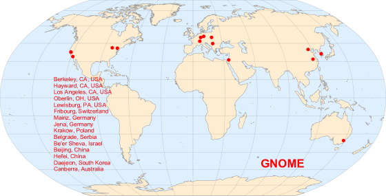
Figure 1: Map and list of locations of GNOME stations. Note that the Fribourg station was moved to Jena in 2018.

In this paper, we review a variety of theoretical models describing sources of transient signals potentially detectable with GNOME. We focus in particular on phenomenological descriptions of the temporal characteristics of the signals that would manifest in the GNOME sensors, which informs our data-analysis strategies.

II Interactions between atomic spins and ultralight bosonic fields

The optical atomic magnetometers (OAMs) [7, 8] comprising GNOME are sensitive to interactions of atomic spins $\boldsymbol{F}$ with hypothetical exotic fields $\boldsymbol{\Upsilon}$, as well as magnetic fields $\boldsymbol{B}$, where $\boldsymbol{F}$ is the total atomic angular momentum. For the exotic spin-dependent interactions considered here, the Hamiltonian has the form:

$$\mathcal{H}_{\Upsilon}=-\sum_{i=e,p,n}{g_{\Upsilon i}\frac{\boldsymbol{S}_{i}}{\left|S_{i}\right|}\cdot\boldsymbol{\Upsilon}}=-\sum_{i}{g_{\Upsilon i}\sigma_{i}\frac{\boldsymbol{F}}{\left|F\right|}\cdot\boldsymbol{\Upsilon}}\,,$$ (1)

where $g_{\Upsilon i}$ is the coupling constant characterizing the interaction of $\boldsymbol{\Upsilon}$ with the fermion spin [where the fermions considered include electrons ($i=e$), protons ($i=p$), and neutrons ($i=n$)], $\sigma_{i}$ is the fractional fermion spin polarization for a given atom (see the Supplemental Material in Ref. [30]), $\boldsymbol{F}$ is the total atomic angular momentum of the atomic state probed, and $\left|S_{i}\right|=1/2$ and $\left|F\right|$ are the maximum spin projections. The exotic-field Hamiltonian $\mathcal{H}_{\Upsilon}$ can be compared to the Zeeman Hamiltonian describing the interaction of atomic spins with a magnetic field:

$$\mathcal{H}_{B}=g_{F}\mu_{B}\boldsymbol{F}\cdot\boldsymbol{B}\,,$$ (2)

where $g_{F}$ is the Landé g-factor, $\mu_{B}$ is the Bohr magneton, and $\boldsymbol{B}$ is the external magnetic field experienced by the atom. Comparing Eqs. (1) and (2), it is evident that the physical manifestations of the ordinary magnetic field coupling and the coupling of exotic fields to spins are analogous. Furthermore, by measuring OAM response to $\boldsymbol{B}$, the response to an exotic field $\boldsymbol{\Upsilon}$ can be inferred [32]. Therefore, we can consider $\boldsymbol{\Upsilon}$ to be a “pseudo-magnetic” field: a field that shifts Zeeman energy levels and generates torques on atomic spins, but does not couple proportionally to spins of different species according to their gyromagnetic ratios (i.e., comparing across different atomic species, $\sum_{i}g_{\Upsilon i}\sigma_{i}/\left|F\right|$ is not proportional to $g_{F}\mu_{B}$). Furthermore, unlike a magnetic field, it may be the case that $\boldsymbol{\Upsilon}$ has nonzero divergence (see, for example, Ref. [33]).

In order to reduce environmental noise from ambient magnetic fields, the atomic vapor cells that contain the gases at the heart of GNOME’s OAMs are placed inside multilayer magnetic shields composed of soft ferrimagnetic or ferromagnetic materials (such as mu-metal) [34]. As noted in Ref. [35], if the exotic field $\boldsymbol{\Upsilon}$ interacts primarily with electron spins, there is an approximate cancellation of the effect of the field $\boldsymbol{\Upsilon}$ on electron spins within the magnetic shield. This is due to the fact that it is the electron spins within shielding materials such as mu-metal that respond to the external magnetic field, so they similarly respond to an electron-coupled field $\boldsymbol{\Upsilon}$. This response generates a corresponding magnetic field approximately cancelling the electron-spin-dependent energy shift within the shield [35]. Consequently, GNOME OAMs are primarily sensitive to exotic field couplings to nuclear spins. At present, GNOME OAMs use alkali atoms such as rubidium (Rb) and cesium (Cs) whose nuclei have valence protons, and thus GNOME predominantly measures interactions of exotic fields with the proton spin $\boldsymbol{S}_{p}$ [36, 37].

The principal hypothesis GNOME has sought to test is that dark matter is composed of ultralight spin-0 bosons known as axions or axion-like particles (ALPs). Such exotic spin-0 bosons are ubiquitous features of the theoretical landscape beyond the Standard Model. The axion originally emerged from a proposed solution to the strong-CP problem [38, 39, 40, 41], the mystery of why nucleon EDMs and CP-violating nuclear electromagnetic moments are many orders of magnitude smaller than nominally predicted by quantum chromodynamics (QCD). Since then, a variety of other beyond-the-Standard-Model theories have emerged predicting similar spin-0 bosons known as ALPs [1, 42, 43, 44, 45]. Axions and ALPs are commonly thought to be ultralight (masses $m_{a}\ll 1\,{\rm eV}$). They can be copiously produced in the early universe [46, 47, 48, 49, 50, 51, 52] and have all the requisite characteristics to be the dark matter [2, 53, 52, 54].

The most commonly considered manifestation of a coupling between an ALP field $\varphi$ and atomic spins is given by the Lagrangian [55]

$$\mathcal{L}_{l}=\frac{{\left(\hbar c\right)}^{3/2}}{f_{l}}J^{\mu}\partial_{\mu}\varphi\,,$$ (3)

where $f_{l}$ is the characteristic energy scale associated with the spin “portal” between ALPs and fermions (the subscript $l$ denoting that the interaction is linear in the ALP field $\varphi$) and $J^{\mu}$ is the axial-vector current for fermions $\psi$,

$$J^{\mu}=\bar{\psi}\gamma^{\mu}\gamma_{5}\psi\,,$$ (4)

where $\gamma^{\mu}$ and $\gamma_{5}$ are Dirac matrices. The corresponding Hamiltonian $\mathcal{H}_{l}$ can be derived from the Euler-Lagrange equations (see, for example, Refs. [1, 56]):

$$\mathcal{H}_{l}\psi=-\frac{{\left(\hbar c\right)}^{3/2}}{f_{l}}\gamma_{0}\gamma^{\mu}\gamma_{5}{\left(\partial_{\mu}\varphi\right)}\psi~{}.$$ (5)

In the nonrelativistic limit, where the spacelike component of the derivative of $\varphi$ is much larger than the timelike component,

$$\mathcal{H}_{li}=-\frac{{\left(\hbar c\right)}^{3/2}}{f_{li}}\frac{\boldsymbol{S}_{i}}{\left|S_{i}\right|}\cdot\boldsymbol{\nabla}\varphi~{},$$ (6)

where the subscript $i$ specifies the interaction with fermion $i=e,p,n$. Comparing Eq. (6) to Eq. (1), we see that the coupling constant for ALPs in the above parameterization is given by $g_{\Upsilon i}={\left(\hbar c\right)}^{3/2}/f_{li}$ and the exotic pseudo-magnetic field is described by $\boldsymbol{\Upsilon}_{l}=\boldsymbol{\nabla}\varphi$. Note that not only does $\mathcal{H}_{l}$ generate an interaction between spins and the spatial gradient of $\varphi$, but $\mathcal{H}_{l}$ also generates an interaction between spins that move with respect to the ALPs, since the momentum is related to the gradient operator via $\boldsymbol{p}=-i\hbar\boldsymbol{\nabla}$. The latter interaction is often referred to as the “axion wind” [57, 55, 5, 58].

We also consider an alternative “quadratic” coupling between spins and the gradient of the intensity of the ALP field, $\boldsymbol{\nabla}\varphi^{2}$ [31]. Whereas the QCD axion associated with the Peccei-Quinn solution to the strong-CP problem [38, 39] generally possesses the linear gradient interaction described by Eqs. (3) and (6) [55], the quadratic gradient interaction can arise in effective field theories predicting ALPs not associated with the QCD sector [59]. It is possible that under certain circumstances (see, for example, Refs. [60, 61, 62]), linear-in-$\varphi$ interactions may be suppressed, and the interaction of photons, electrons and nuclei with scalar fields starts at the quadratic order, $\varphi^{2}$. A very important consequence of such a modification is the relaxation of the most stringent astrophysics bounds compared to the linear case [59], opening up a parameter space for the direct searches of $\varphi^{2}$ coupling to spins. Also note that quadratic-in-$\varphi$ interactions are required for complex-valued $\varphi$, as is the case for the Q-ball scenario discussed in Sec. IV.3. Furthermore, there are novel experimental signatures and modalities that can be employed to search for the quadratic-in-$\varphi$ interactions [63].

The Lagrangian describing the quadratic gradient coupling between an ALP field and atomic spins is given by [31]

$$\mathcal{L}_{q}=\frac{\hbar^{2}c^{2}}{f_{q}^{2}}J^{\mu}\partial_{\mu}\varphi^{2}~{}.$$ (7)

The corresponding Hamiltonian is described by

$$\mathcal{H}_{q}\psi=-\frac{\hbar^{2}c^{2}}{f_{q}^{2}}\gamma_{0}\gamma^{\mu}\gamma_{5}{\left(\partial_{\mu}\varphi^{2}\right)}\psi\,,$$ (8)

and in the nonrelativistic limit the Hamiltonian describing the interaction of $\varphi$ with the spin of fermion $i$ is approximately

$$\mathcal{H}_{qi}=-\frac{\hbar^{2}c^{2}}{f_{qi}^{2}}\frac{\boldsymbol{S}_{i}}{\left|S_{i}\right|}\cdot\boldsymbol{\nabla}\varphi^{2}~{}.$$ (9)

Comparing Eq. (9) to Eq. (1), we see that the coupling constant for ALPs in the above parameterization is given by $g_{\Upsilon i}={\left(\hbar c\right)}^{2}/f_{qi}^{2}$ and the exotic pseudo-magnetic field is described by $\boldsymbol{\Upsilon}_{q}=\boldsymbol{\nabla}\varphi^{2}$.

It is of interest to note the discrete symmetry properties of the interactions described by Eqs. (6) and (9). Consider as a reference the discrete symmetry properties of the standard Zeeman interaction of Eq. (2). The atomic angular momentum $\boldsymbol{F}$ is even under parity (P-even), since it is an axial- or pseudo-vector, and odd under time-reversal (T-odd), since angular momentum reverses its sign when time runs backward. The magnetic field $\boldsymbol{B}$, generated by current flow, is also P-even and T-odd, and thus $\mathcal{H}_{B}$ is P- and T-even. For the linear gradient interaction of Eq. (6), the pseudoscalar ALP field $\varphi$ is P-odd and T-odd and the gradient $\boldsymbol{\nabla}$ is P-odd and T-even, and thus $\boldsymbol{\nabla}\varphi$ is a P-even, T-odd quantity, matching the discrete symmetry properties of the magnetic field. Consequently, $\mathcal{H}_{l}\propto\boldsymbol{S}\cdot\boldsymbol{\nabla}\varphi$ is P- and T-even. On the other hand, for the quadratic gradient interaction of Eq. (9), $\boldsymbol{\nabla}\varphi^{2}$ is P-odd and T-even because of the extra factor of the ALP field $\varphi$, which means that the quantity $\boldsymbol{S}\cdot\boldsymbol{\nabla}\varphi^{2}$ is P- and T-odd. Based on CPT invariance (where C is the charge conjugation symmetry), it follows that $\mathcal{H}_{q}$ describes a CP-violating interaction, and as a result could play a role in baryogenesis [64].

III GNOME overview

The idea of the GNOME experiment is to carry out synchronous measurements of spin-dependent interactions using OAMs operating within magnetically-shielded environments in distant locations. In this section we review the basic feature of the GNOME network, give an overview of the data collected so far, and describe ongoing improvements to the GNOME sensors that will significantly enhance the network sensitivity.

III.1 GNOME magnetometers

As mentioned above, OAMs utilize the interaction of atomic spins with external magnetic fields [7]. Typically, alkali metal vapors, contained in glass cells, are used for the measurements. To prevent spin-depolarizing collisions with cell walls, which can limit the OAM sensitivity, either the walls are coated with special (e.g., paraffin) layer or the cells are filled with an additional inert gas (e.g., noble gas) to slow down diffusion. In OAMs, the atoms are optically polarized, resulting in optical anisotropy of the medium. As the spins of the polarized atoms precess due to a nonzero magnetic field (or, perhaps, due to an exotic field coupled to atomic spins), detection of the corresponding change in optical properties of the medium provides quantitative information about the field. The signals of the GNOME magnetometers are recorded using a custom data acquisition (DAQ) system [65], providing accurate timing from the Global Positioning System (GPS).

In the first incarnation of the GNOME, various OAMs employed different elements (Rb and Cs) and were based on different techniques; spin-exchange-relaxation-free (SERF) [66], M_x [67], and nonlinear-magneto-optical-rotation (NMOR) [68] magnetometers were used for the measurements. On the one hand, this diversity offers flexibility, opens a greater range of theoretical parameter space for exploration, and improves the robustness of the network. On the other hand, it results in sensors having different sensitivities and bandwidths, which complicates data analysis. In general, however, magnetometers used in the GNOME have an operational sensitivity better than 1 pT/$\sqrt{\text{Hz}}$, corresponding to a sensitivity to Zeeman energy shifts below 10^-17 eV/$\sqrt{\text{Hz}}$, and bandwidths up to 100 Hz [29].

Although OAMs enable searches for non-magnetic spin couplings, the devices are highly sensitive to magnetic fields. Therefore, despite shielding from the external environment, uncontrollable magnetic disturbances are a significant source of noise. In order to reduce magnetic noise, the next generation of the GNOME experiment (Advanced GNOME) is using comagnetometers [69, 70]: sensors with limited sensitivity to magnetic fields that still maintain sensitivity to non-magnetic spin couplings. Comagnetometers are briefly described in Sec. III.5.

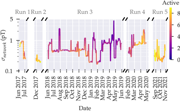
Figure 2: One-day rolling average of the GNOME noise level according to Eq. (10) over the course of the first five Science Runs. The standard deviation at each magnetometer is calculated using the data for one second. Then this information is averaged for one hour. The color of the line indicates the number of active stations as indicated on the color map legend at the upper right.

III.2 Monitoring of glitches

While by its nature the GNOME can suppress uncorrelated noise and false positive events, additional measures are implemented in the network to further increase the data quality and trustworthiness of each station. In order to veto signatures in the data which might have been produced by technical issues or changing experimental conditions (e.g., mechanical shocks, magnetic or electric pulses from neighboring technical devices), each GNOME station features a tailored automated system to continuously check for environmental perturbations. The system is based on the Arduino microcontroller board MEGA 2560 additionally equipped with the Arduino 9 Axes motion shield (magnetometer, accelerometer and gyroscope, three axes each) in a separate “sensor box”. The sensor box is mounted on the optical table of the GNOME station near the magnetic shielding. In this way, it can check for mechanical shocks or vibration of the optical setup. In addition, the system features additional analog voltage inputs, which are used to monitor the operational status of the station (e.g., magnetometer signal amplitude, error signal of the magnetometer feedback and/or the laser lock, readings of temperature sensors, and signals of a photo diode monitoring laser or ambient light power). For each GNOME station, depending on the specific setup, the system is set to monitor its critical parameters.

A dedicated Python-based software allows the system to display, save, and define “sane” ranges for all monitored parameters. If one of the parameters falls out of the “sane” range, the system will output a signal to the DAQ system indicating the data recorded meanwhile should be rejected in data analysis. The software writes a log file allowing one to trace back the event to the individual monitored parameter. It is also possible to set alarms to notify station operators about irregularities over email and/or the Telegram app.

III.3 Calibration pulses

A possible concern with the continuous operation of the magnetometers over the course of several months is variation in the calibration and bandwidth of the detectors. Such variations could result from drifts in laser power, laser frequency, or temperature of the vapor cells. To monitor this, a series of oscillating magnetic fields are periodically applied to each magnetometer station via coils inside the magnetic shields. The frequency of the applied magnetic field is stepped from 1 to 180 Hz over the course of 9 s using a programmable function generator. During the most recent experimental campaign (Science Run 5), the pulse sequence was applied hourly. The response of the magnetometers at the different frequencies provides a convenient check on the operation of the magnetometers as well as a method for measuring the frequency response and bandwidth of the detectors. The pulses also provide a test of the timing of the stations. The pulses are triggered by the GPS pulse-per-second (pps) signal of the GNOME DAQ system or a time synchronized computer clock. These tests indicate that the stations are synchronized at a level of better than the sample period, $T_{\textrm{samp}}=1/512$ s.

III.4 The GNOME experiment so far

To date, the GNOME collaboration has completed five “Science Runs” as well as a number of test and calibration runs. According to Eqs. (6) and (9) and the surrounding discussion in Sec. II, GNOME sensors seek to measure characteristic global patterns of pseudo-magnetic fields $\boldsymbol{\Upsilon}$. Typically, GNOME magnetometers are sensitive to the projection of $\boldsymbol{\Upsilon}$ along a particular sensitive axis. Thus the amplitudes of signals from exotic fields $\boldsymbol{\Upsilon}$ scale proportionally to $\hat{\boldsymbol{m}}\cdot\boldsymbol{\Upsilon}$, where $\hat{\boldsymbol{m}}$ is a unit vector pointing along the sensitive axis of a magnetometer. Since the direction of the field $\boldsymbol{\Upsilon}$ is essentially unknown, in order to assess the sensitivity of the GNOME, this directional sensitivity must be taken into account. Additionally, the various parameters of individual sensors must be considered along with the relationship between the sensor response and the underlying physical theory (which must account for atomic and nuclear structure [36, 37]). These issues are discussed in more detail in Refs. [71, 30, 72].

A summary of the network performance for the five GNOME Science Runs is shown in Fig. 2. Since the GNOME data can be utilized in different ways to test different exotic physics hypotheses, discussed in Sec. IV, for simplicity we adopt for the summary a relatively simple, model-independent evaluation. The plot in Fig. 2 shows the one-hour-average noise level as defined by

$$\sigma{{}_{\mbox{\scriptsize network}}}\equiv\sqrt{\frac{1}{\sum_{j}\sigma_{j}^{-2}}}\,,$$ (10)

where $\sigma_{j}$ is the variance of magnetometer $j$, calculated using the standard deviation for each second of data. As can be seen from Fig. 2, the GNOME experiment has accumulated over a year of data sensitive to pseudo-magnetic fields with equivalent magnitudes $\lesssim\textrm{pT}$ that can be searched for a variety of exotic physics signals.

III.5 Advanced GNOME: noble gas comagnetometers

The further development of the GNOME experiment focuses on the diversification and upgrade of the sensors implemented in the network. There are three main directions for the improvement of sensors: enhancing their sensitivity, increasing their bandwidth, and expanding the types of couplings probed. Although a number of various experimental techniques could be used for GNOME sensors (e.g., spin-based amplifiers [73], noble gas masers [74, 75], dual-species nuclear-spin comagnetometers [76, 77], alkali comagnetometers [78, 79, *kimball2023GDMerratum, 81], liquid-state NMR comagnetometers operating in the zero-to-ultralow field (ZULF) regime [82, 83], etc.), efforts are presently focused on developing self-compensating noble-gas-alkali-metal comagnetometers [69, 70] for implementation in the “Advanced GNOME” experiment [32, 84].

In addition to the coupling of exotic fields to proton spins, which was the only coupling probed at a competitive level by the first-generation GNOME [30], self-compensating noble-gas-alkali-metal comagnetometers can also probe both neutron and electron spin couplings. The ability to measure neutron spin couplings to $\boldsymbol{\Upsilon}$ comes from the fact that the noble gases (such as ³He) employed in these sensors have nuclei with valence neutrons [36]. However, the reason for the ability of these sensors to measure electron spin couplings is somewhat more subtle. If we assume that $\boldsymbol{\Upsilon}$ couples primarily to electron spins, then the ferromagnetic (or ferrimagnetic) shielding responds to $\boldsymbol{\Upsilon}$ by creating an induced magnetic field that cancels the effect of $\boldsymbol{\Upsilon}$ on electrons within the shield where the vapor is located [35]. However, if we assume no coupling of $\boldsymbol{\Upsilon}$ to neutron spins, then neutrons will respond to the induced magnetic field from the shields and thus a detectable effect is generated. This further highlights the advantages of comagnetometry for exotic physics searches with the GNOME. At sub-Hz frequencies, the sensitivity of the comagnetometer is also significantly improved by the suppression of the magnetic field response due to the self-compensation regime in which the comagnetometer is operated.

Initial tests of Advanced GNOME sensors demonstrate a sensitivity at the level of 10^-21 eV/$\sqrt{\mathrm{Hz}}$ (at 1 Hz) for exotic fields coupling to neutron spins, and about 10^-19 eV/$\sqrt{\mathrm{Hz}}$ (at 1 Hz) for the proton spin coupling (surpassing that of GNOME magnetometers by a factor of 100), see Fig. 3. For the electron spin couplings, the expected sensitivity is comparable to the sensitivity of the first-generation GNOME magnetometers to the proton exotic spin couplings. The noble-gas-alkali-metal comagnetometers have an optimal sensitivity to the nuclear spin couplings for frequencies below a few hertz. However, enhanced sensitivity to exotic fields (as compared to the first-generation of GNOME magnetometers) is expected over the whole bandwidth of the ordinary magnetometers, even at frequencies for which the comagnetometer performance is sub-optimal.

The Advanced GNOME sensors also bring another significant qualitative advantage for exotic physics searches. The difference in the response to the magnetic and non-magnetic spin couplings can be used to discriminate events of magnetic origin from those driven by non-magnetic spin couplings, just from a single sensor readout [32]. Although ultimate verification of a global exotic physics event will rely on the correlation between signals observed in multiple GNOME stations, more effective discrimination between magnetic and non-magnetic signals will enable efficient suppression of the “false positive” rate and therefore improve the overall sensitivity of the network.

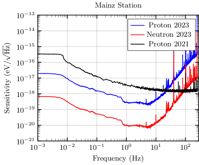
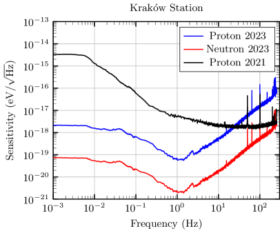
Figure 3: Sensitivities of Advanced GNOME stations in Mainz (left) and Kraków (right) obtained during a Test Run in January 2023, compared with the typical sensitivity of the first-generation GNOME stations during Science Run 5 (see Fig. 2). Red curves: sensitivities of the comagnetometers to the neutron exotic spin couplings; blue curves: sensitivity of the comagnetometers to the proton spin couplings; black curves: magnetometer sensitivities to exotic proton couplings. The sensitivities are presented in terms of Zeeman-like energy splitting generated by the considered perturbation. The presented data sets were undersampled for illustration purposes.

IV Search targets and their signals

By analyzing correlations between signals from the geographically separated magnetometers and comagnetometers comprising GNOME, it is possible to probe a wide variety of exotic beyond-the-Standard-Model hypotheses. In this section we survey some exotic physics scenarios that can be searched for using GNOME data and highlight examples of their particular temporal signatures.

IV.1 Axion domain walls

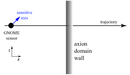
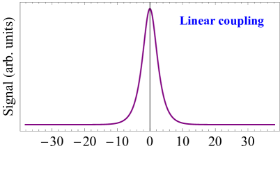
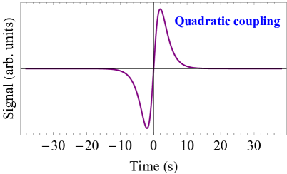
Figure 4: Upper diagram: schematic depiction of a GNOME sensor passing through an ALP domain wall (thickness $\approx R_{E}/10$), indicating with the long black arrow the trajectory of the sensor along $\boldsymbol{v}$ (parallel to $\boldsymbol{k}$, along $\hat{\boldsymbol{x}}$, $v\approx 10^{-3}c$) and the sensitive axis of a GNOME sensor (blue arrow, tilted at $45^{\circ}$ to $\hat{\boldsymbol{x}}$). The plots below show example signals due to the linear spin coupling (middle plot) and quadratic spin coupling (lower plot) from an ALP-domain-wall encounter corresponding to the schematic at top.

The first proposed search targets for GNOME were axion or ALP domain walls [31, 28]. Domain walls are topological defects that form between regions of space in which the ALP field possesses different, but energy-degenerate, vacuum states [85, 86]. Such a scenario arises due to the non-trivial vacuum topology that ALP fields typically possess: there can be multiple local field energy minima (and corresponding vacuum states) that, in the abstract space describing the field, are not “simply connected” in a topological sense [87]. When spontaneous symmetry breaking occurs in the early universe, different regions of space (domains) acquire different vacuum states. The domain walls are the field configurations at the boundaries between these domains. In order for the ALP field to transition from one energy minimum to another across these boundaries, the ALP field necessarily acquires values above those corresponding to the minimum energy. These non-vaccuum states are associated with considerable potential energy, and the change of the field over space means that the ALP field has a nonzero gradient.

IV.1.1 Theoretical description

ALP domain walls are macroscopic field configurations that could be stable and long lived, and continue to exist today [86]. They can be of astrophysical extent, potentially much larger than the size of Earth. If the ALP field primarily manifests in the form of domain walls, the associated energy density would be concentrated into compact spatial regions. While in most theoretical models such domain walls are unstable [85, 88], in some other models [31, 89, 86] domain walls can compose a significant fraction of dark matter. These objects can be considered virialized in the galaxy according to the standard halo model (SHM). Based on this assumption, the rate and duration of the ALP domain wall encounters can be estimated. A region of theoretically plausible parameter space is expected to have an average encounter rate with Earth of a year or less [31, 89]. This opens the possibility to directly search for such encounters. Atomic magnetometers and comagnetometers are sensitive to domain walls, since the ALP-field gradient can interact with the spin of electrons, neutrons and protons [see Eqs. (6) and (9)].

IV.1.2 Signal model

Consider an ALP domain wall in the $yz$-plane ($x=0$) separating two degenerate ALP vacuum states as pictured in the upper diagram in Fig. 4. The solution of the field equations for $\varphi$ yields [90, 31, 30]

$$\varphi(x)=\varphi_{0}\arcsin{\left[\tanh{\left(x/\lambda_{c}\right)}\right]}\,,$$ (11)

where $\varphi_{0}$ is a constant proportional to the spontaneous symmetry-breaking scale associated with the ALP and $\lambda_{c}=\hbar/{\left(m_{a}c\right)}$ is the Compton wavelength of the ALP of mass $m_{a}$. Atomic spins can interact with the ALP field through the linear and quadratic gradient interactions of Eqs. (6) and (9), which can be described by the pseudo-magnetic fields

$$\boldsymbol{\Upsilon}_{l}=\boldsymbol{\nabla}\varphi(x)=\frac{\varphi_{0}}{\lambda_{c}}\operatorname{sech}{\left(x/\lambda_{c}\right)}\,\hat{\boldsymbol{x}}$$ (12)

and

$$\boldsymbol{\Upsilon}_{q}=\boldsymbol{\nabla}\varphi^{2}(x)=\frac{2\varphi_{0}^{2}}{\lambda_{c}}\arcsin{\left[\tanh{\left(x/\lambda_{c}\right)}\right]}\operatorname{sech}{\left(x/\lambda_{c}\right)}\,\hat{\boldsymbol{x}}\,,$$ (13)

respectively. The signal measured by a GNOME sensor is $\propto\hat{\boldsymbol{m}}\cdot\boldsymbol{\Upsilon}$, where $\hat{\boldsymbol{m}}$ is directed along the sensitive axis of the magnetometer. The expected time-dependent lineshapes for the linear and quadratic couplings are shown in the lower plots of Fig. 4. While all the GNOME sensors experience a common transient pseudo-magnetic field $\boldsymbol{\Upsilon}$, because of the varying directions of their sensitive axes $\hat{\boldsymbol{m}}$ (as well as differences in the magnetometers employed), the signals in different sensors would have varying amplitudes and signs. For a given relative velocity between the ALP domain wall and Earth, there is a characteristic signal timing and amplitude pattern that can be used to distinguish true domain-wall-crossing events from spurious noise [71, 91, 30]. Once an event is detected, one can relate the signal properties (width and the amplitude of the signal, as well as the inferred expected distribution of domain walls) to ALP parameters, including the mass of the ALP and the interaction and symmetry-breaking scales [30].

The GNOME collaboration has developed data analysis algorithms to search for ALP domain walls [71, 91], and has completed a full analysis of the data from Science Run 2 carried out in 2017 [30]. Our searches did not find any statistically significant signals above background that could point to the existence of ALP domain walls. Consequently, our results can be interpreted as constraints on the properties of ALP domain walls. The excluded (model-dependent) ALP parameter space covers masses in the range $\sim 10^{-15}-10^{-7}$ eV [30]. A new analysis procedure is currently being developed to improve on the sensitivity to narrower domain wall widths with respect to our previous work [30]. The new analysis is based on a preselection of candidate signals groups occurring within a given time window. Then each group is tested for consistency with the domain wall crossing model. This allows an efficient scrutiny of the data compared to the previous method. In Ref. [30] all possible domain wall configurations were scanned and their agreement with the data were evaluated. The new procedure results in a comparatively less computer-intensive routine.

IV.2 Axion stars

Instead of the ALP dark matter being primarily in the form of topological defects such as domain walls as discussed above in Sec. IV.1, it may be the case that inhomogeneities in the dark matter distribution provide seeds that enable ALP self-interactions or gravity to attract together a large local density of ALPs, thereby forming a spherical bound-state (see Refs. [92, 93, 94, 95] and references therein). Such spherical bound states are referred to as axion or ALP stars, and they may constitute a significant fraction of the dark matter density [92]. Under certain conditions, ALP stars are stable under perturbations and radiative decay [96, 97, 98, 99], and can be efficiently formed in the early Universe [100, 101, 102, 103]. The extensive theoretical studies of ALP stars to determine their evolution, stability, and characteristic radii and masses for different models of the ALP self-interaction establish that ALP stars are, indeed, a plausible dark matter scenario [92, 104, 105]. As described in Ref. [106], ALP stars are a compelling search target for the GNOME, since there is a range of masses and radii for ALP stars (not ruled out by existing empirical observations) for which the terrestrial encounter rate can be sufficiently high (at least once per year) that a detection would be feasible. ALP stars can interact with atomic spins via the linear or quadratic gradient interactions [Eqs. (6) and (9)]. Thus if an ALP star passed through Earth, it would cause oscillatory pseudo-magnetic field pulses in GNOME sensors that, in principle, could be within the sensitivity range of GNOME [106].

IV.2.1 Theoretical description

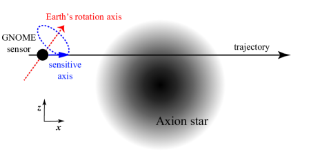
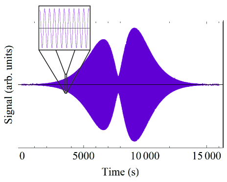
Figure 5: Upper diagram: schematic depiction of a GNOME sensor passing through an ALP star, indicating with the long black arrow the trajectory of the sensor along $\boldsymbol{v}$ (parallel to $\boldsymbol{k}$, along $\hat{\boldsymbol{x}}$), the initial direction of the sensitive axis of the GNOME sensor (blue arrow, along $\hat{\boldsymbol{x}}$), and the axis of Earth’s rotation (dashed red arrow, $45^{\circ}$ to the $x$-axis). Lower plot: example signal due to the linear spin coupling [Eq. (19)] from an ALP star passage corresponding to the above schematic. For this example, the ALP star radius $R\approx 200R_{E}$, $v=10^{-3}c$, and at $t=0$ the sensor is located at ${\left(x_{0},y_{0},z_{0}\right)}={\left(2R,0,R/2\right)}$, where the origin is defined to be the center of the ALP star. The ALP field oscillation frequency is chosen to be $\omega=2\pi\times 10\,{\rm Hz}$, and we assume $\omega\approx\omega_{c}$, neglecting the binding energy. The ALP-star signal in the plot is based on the exponential model, Eq. (16). The inset plot shows an $\approx 1~{}{\rm s}$ long segment of the simulated signal.

Axion or ALP stars held together via self-interactions are called oscillons [107] or axitons [108]. There have been a number of theoretical studies of such composite systems, and a few general features are observed. Models of oscillons and axitons demonstrate that they can persist in a stable or quasi-stable regime [109, 110, 111], however if the ALP density is too large, they tend to radiate ALP waves and lose mass [92]. Sufficiently dilute ALP stars can be stable over long time scales [109, 110, 112]. The ALP fields bound in the form of oscillons have a characteristic field oscillation frequency $\omega$ which is somewhat smaller than the ALP Compton frequency $\omega_{c}$. This stems from the fact that, while free ALPs oscillate at the Compton frequency $\omega_{c}$, because the energy of the ALPs in the star is reduced by a binding energy $\epsilon_{b}$, the oscillation frequency of ALPs in the oscillon is given by

$$\omega=\omega_{c}-\epsilon_{b}/\hbar~{}.$$ (14)

This is a key difference between the ALP domain walls considered in Sec. IV.1 and the ALP stars considered here: the ALP field of the domain wall does not oscillate, being a topological defect related to the ALP field potential energy, whereas the ALP field of the star does oscillate, since most of the field energy is in the form of kinetic energy. The mass $M$ of an oscillon is $M\approx N{\left(m_{a}-\epsilon_{b}/c^{2}\right)}$, where $N$ is the number of ALPs in the star.

Alternatively, axion stars could be held together by gravity [113, 114, 115, 116, 96, 97, 98, 99]. However, in this case it may be expected that gravitational tidal forces due to the Sun, Earth, and other bodies in the solar system could cause distortions and disruptions of the axion star [117], complicating the details of the shape profile in ways that are difficult to predict. Thus, for simplicity, here we focus on the oscillon or axiton models where self-interactions stronger than gravity dominate.

IV.2.2 Signal model

A number of different approximate analytic wavefunctions for ALP stars have been studied in the literature (see Ref. [95] for a review). Two of the more widely used radial wavefunctions $\Psi(r)$, where $r$ is the radial distance from the center of the ALP star, are the Gaussian approximation,

$$\Psi(r)=\sqrt{\frac{N\kappa^{3}}{\pi^{3/2}R^{3}}}e^{-\kappa^{2}r^{2}/(2R^{2})}\,,$$ (15)

and the exponential approximation,

$$\Psi(r)=\sqrt{\frac{N\kappa^{3}}{\pi R^{3}}}e^{-\kappa r/R}\,,$$ (16)

where $R$ is the characteristic radius of the ALP star enclosing 99% of its mass and $\kappa$ is a numerical parameter ($\kappa=2.8$ for the Gaussian wavefunction and $\kappa=4.2$ for the exponential wavefunction [95]). In Ref. [95] it is argued that, in fact, a more accurate description of an ALP star in many relevant scenarios is given by a “linear-plus-exponential” wave function:

$$\Psi(r)=\sqrt{\frac{N\kappa^{3}}{7\pi R^{3}}}{\left(1+\frac{\kappa r}{R}\right)}e^{-\kappa r/R}~{}.$$ (17)

In any case, the ALP field as observed from the reference frame of a GNOME sensor is given by

$$\varphi(\boldsymbol{r},t)=\Psi(r)\cos{\left(\boldsymbol{k}\cdot\boldsymbol{r}-\omega t+\theta\right)}\,,$$ (18)

where $\boldsymbol{k}$ is the ALP wave vector, $\boldsymbol{r}$ is the distance from the center of the ALP star to the sensor, and $\theta$ is a random phase. Since the ALP field in the star is essentially a Bose condensate with long coherence time [92], we can treat the phase $\theta$ as constant throughout the duration of the passage of the GNOME sensor through the ALP star, and for simplicity in the following discussion we set $\theta=0$.

The expected signal in a GNOME sensor can be calculated based on the exotic pseudo-magnetic fields $\boldsymbol{\Upsilon}_{l}=\boldsymbol{\nabla}\varphi$ and $\boldsymbol{\Upsilon}_{q}=\boldsymbol{\nabla}\varphi^{2}$ obtained from the expression (18), where (as above) the subscripts denote the linear or quadratic fields:

$$\boldsymbol{\Upsilon}_{l} ={\left(\boldsymbol{\nabla}\Psi\right)}\cos{\left(\boldsymbol{k}\cdot\boldsymbol{r}-\omega t\right)}-\boldsymbol{k}\Psi(r)\sin{\left(\boldsymbol{k}\cdot\boldsymbol{r}-\omega t\right)}\,,$$

$$={\frac{\partial\Psi}{\partial r}}\cos{\left(\boldsymbol{k}\cdot\boldsymbol{r}-\omega t\right)}\hat{\boldsymbol{r}}-\frac{m_{a}v}{\hbar}\Psi(r)\sin{\left(\boldsymbol{k}\cdot\boldsymbol{r}-\omega t\right)}\hat{\boldsymbol{k}}\,,$$ (19)

and

$$\boldsymbol{\Upsilon}_{q} ={\left(\boldsymbol{\nabla}\Psi^{2}\right)}\cos^{2}{\left(\boldsymbol{k}\cdot\boldsymbol{r}-\omega t\right)}-2\boldsymbol{k}\Psi(r)\cos{\left(\boldsymbol{k}\cdot\boldsymbol{r}-\omega t\right)}\sin{\left(\boldsymbol{k}\cdot\boldsymbol{r}-\omega t\right)}\,,$$

$$=2\Psi(r){\frac{\partial\Psi}{\partial r}}\cos^{2}{\left(\boldsymbol{k}\cdot\boldsymbol{r}-\omega t\right)}\hat{\boldsymbol{r}}-\frac{2m_{a}v}{\hbar}\Psi(r)\cos{\left(\boldsymbol{k}\cdot\boldsymbol{r}-\omega t\right)}\sin{\left(\boldsymbol{k}\cdot\boldsymbol{r}-\omega t\right)}\hat{\boldsymbol{k}}\,.$$ (20)

There are two generally non-orthogonal components of the signal along $\hat{\boldsymbol{k}}$ and $\hat{\boldsymbol{r}}$, which change in magnitude as the GNOME sensor passes through the ALP star. Note that the sensitive axis $\hat{\boldsymbol{m}}$ changes in time as Earth rotates, so this can introduce additional time dependence of the signal which is $\propto\hat{\boldsymbol{m}}\cdot\boldsymbol{\Upsilon}$. Figure 5 shows an example of a simulated signal in a GNOME sensor passing through an ALP star for a particular set of parameters. Both the direction and magnitude of $\boldsymbol{\Upsilon}$ change as the GNOME sensor passes through the ALP star, as well as the direction of $\hat{\boldsymbol{m}}$, leading to the somewhat complicated time-dependence.

The GNOME collaboration is currently developing an analysis method to search for ALP stars exhibiting this type of signal using the excess power statistic [118].

IV.3 Q-balls

Another class of compact composite dark matter objects are Q-balls or Q-stars [119, 120, 121, 122]. Q-balls are nontopological solitons: bound states of a complex scalar field $\varphi$. If complex scalar field $\varphi$ obeys global $U(1)$ symmetry, and has a non-zero net charge density Q, the self-interaction of the scalar field makes it energetically favorable for the field to fragment into clumps, called Q-balls [123, 124]. In some models, Q-balls could comprise the entirety of dark matter [125, 126]. There are also various theoretical extensions of the Q-ball concept, involving, for example, multiple scalar fields [127] or local $U(1)$ symmetries instead of global [128]. The distinction between Q-balls and ALP stars is somewhat subtle. Q-balls, because of the global $U(1)$ symmetry, are true solitons since they are stable due to the conserved charge associated with $\varphi$. On the other hand, oscillons, our model for ALP stars, represent “quasi-solitons” because, while under particular conditions they can be very long-lived, they are technically unstable. The Q-ball is composed of a complex field, whereas the oscillon is composed of a real field. For both Q-balls and oscillons, an attractive potential is required for formation. As we see in the following, the differences between the underlying theoretical models describing oscillons and Q-balls lead to distinct experimental signatures in GNOME.

IV.3.1 Theoretical description

The complex scalar field of a Q-ball takes the form [119]

$$\varphi(\boldsymbol{r},t)=\Psi(r)e^{i\omega t}\,,$$ (21)

where $\omega\lesssim\omega_{c}$ is the angular oscillation frequency. The stability of the Q-ball is a consequence of its conserved charge $Q$

$$Q=\frac{\omega}{\hbar^{2}c^{3}}\int\left|\varphi(\boldsymbol{r},t)\right|^{2}d^{3}\boldsymbol{r}~{}.$$ (22)

The necessary conditions for Q-ball formation are that $Q\neq 0$ averaged over the whole space and the existence of a self-interaction potential $U(\Psi)$ possessing at least two distinct minima at $\Psi=0$ and at $\Psi=\Psi_{0}$ [119, 120, 121, 122]. In this case, there are regions of space with different vacuum energy values, and the regions where $\Psi=\Psi_{0}$ can deform but not disappear because of the conserved charge $Q$. A characteristic feature of the Q-ball is that the potential energy of the field, $U{\left(\Psi\right)}$, is nonzero in the Q-ball’s transitional surface region where the field goes from $\Psi=0$ to $\Psi=\Psi_{0}$. Therefore the Q-ball’s energy is minimized when its surface area is minimized, leading to a spherical bound-state. Furthermore, it is energetically favorable for the constituent particles corresponding to the field $\varphi$ (ALPs in our considered case) to remain within the Q-ball in the case where $\omega\lesssim\omega_{c}$, since ALPs inside the Q-ball have energy $\hbar\omega$ while those outside the Q-star have energy $\hbar\omega_{c}$. The values of $\omega^{2}$ and $\omega_{c}^{2}$ are proportional to $\partial^{2}U/\partial\Psi^{2}$ at the respective potential minima inside ($\Psi=\Psi_{0}$) and outside ($\Psi=0$) the Q-ball, and can thus be different [119, 122]. The condition $\omega\lesssim\omega_{c}$ ensures stability of the Q-star with respect to radiative decay via ALP emission.

IV.3.2 Signal model

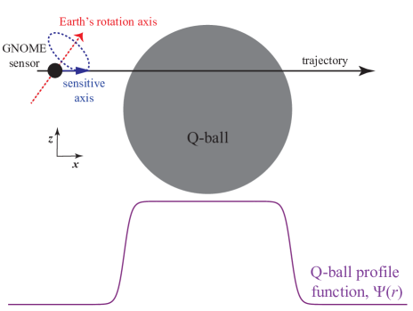
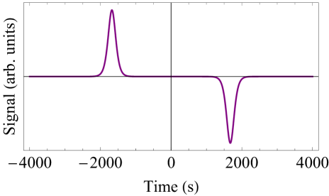
Figure 6: Upper diagram: schematic depiction of a GNOME sensor passing through an astronomically large Q-ball (radius $\approx 100R_{E}$), indicating with the long black arrow the trajectory of the sensor along $\boldsymbol{v}$ (parallel to $\boldsymbol{k}$, along $\hat{\boldsymbol{x}}$, $v\approx 10^{-3}c$), the initial direction of the GNOME-sensor sensitive axis (blue arrow, along $\hat{\boldsymbol{x}}$), and the axis of Earth’s rotation (dashed red arrow, $45^{\circ}$ to the $x$-axis). The purple curve below shows the profile function of the Q-ball. Lower plot: example signal due to the quadratic spin coupling from a Q-ball passage corresponding to the above schematic.

The precise form of $\Psi(r)$ depends on details of the potential function, and, although there are special forms of $U(\Psi)$ admitting analytic solutions [129, 130, 131], in general numerical computation is required. However, there have been a number of analyses, for example Refs. [132, 133, 134], that have derived useful approximate radial profile functions that closely correspond to numerical solutions. For simplicity of mathematical description, here we adopt the form given by Ref. [132],

$$\Psi(r)=\frac{C_{0}}{\sqrt{1+C_{1}\cosh{\left(\alpha r\right)}}}\,,$$ (23)

where $C_{0}$, $C_{1}$, and $\alpha$ are constants determined by fitting to numerical solutions for various potentials and values of $Q$ and $\omega$. In contrast to the cases of ALP domain walls and ALP stars as described in Secs. IV.1 and IV.2, for the complex-valued field $\varphi(r)$ forming Q-balls [Eq. (21)], any couplings of spins to $\varphi(r)$ must be quadratic in $\varphi(r)$ [135]. This is required in order to respect the global $U(1)$ symmetry that endows the Q-ball with its charge: from a mathematical point-of-view, interactions must involve products of $\varphi(r)$ and $\varphi(r)^{*}$ to give a real-valued energy. Therefore we consider the pseudo-magnetic field $\boldsymbol{\Upsilon}_{q}$ arising from the quadratic interaction,

$$\boldsymbol{\Upsilon}_{q} =\boldsymbol{\nabla}{\left|\varphi(r,t)\right|}^{2}=\boldsymbol{\nabla}\Psi^{2}(r)\,,$$ (24)

$$=\alpha C_{0}^{2}C_{1}\frac{\sinh{\left(\alpha r\right)}}{\left[1+C_{1}\cosh{\left(\alpha r\right)}\right]^{2}}\hat{\boldsymbol{r}}\,.$$ (25)

Figure 6 shows a schematic example of the signal that would be measured by a GNOME sensor passing through a Q-ball. In contrast to the ALP star considered in Sec. IV.2, the signal of the Q-ball does not exhibit oscillatory behavior, and is in fact more similar to the signature of an ALP domain wall considered in Sec. IV.1. However, there is the notable difference that for a Q-ball there should be two correlated time-separated signals corresponding to entry and exit from the $\Psi=\Psi_{0}$ region, offering a unique signature pattern that can be exploited for noise rejection.

Note that the signal pattern in GNOME corresponding to a Q-ball encounter (Fig. 6) closely resembles that from two consecutive domain-wall encounters (Fig. 4), or a domain-wall encounter with a quadratic coupling in the case of a domain wall that is “thick” compared to the size of Earth. This suggests that our data analysis strategies applied to domain-wall searches [71, 91, 30] can be adapted to the case of Q-balls. Development of an analysis algorithm based on this concept is under way.

IV.4 Dark-matter field fluctuations

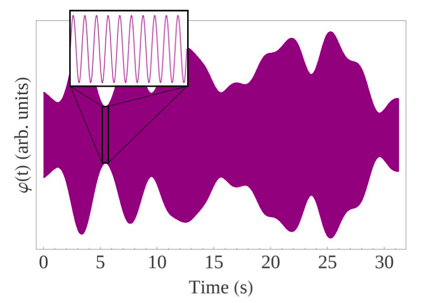
Figure 7: Visualisation of the dark matter field oscillating at its Compton frequency with fluctuations of the envelope function.

Unlike the compact dark matter objects described so far, in this section we consider the more commonly assumed model for UBDM, namely that the UBDM field is spread more evenly throughout the galactic halo volume and not concentrated in large, compact objects. Due to their ultralight nature and (if they constitute a sizable fraction of the dark matter) their enormous number density, ALPs can be treated as classical plane waves. In the standard halo model (SHM), ALPs are virialized in the gravitational potential of the Milky Way, and their energy is given by $\hbar\omega\approx m_{a}c^{2}+m_{a}v^{2}/2$ where $\omega$ is the observed ALP field oscillation frequency and $v\sim 10^{-3}c$ is the ALP velocity. Due to the ALPs’ randomized velocities, different ALP field modes interfere with one another resulting in a net field that stochastically fluctuates on a characteristic time scale given by the ALP field coherence time $\tau{{}_{\mbox{\scriptsize coh}}}\sim\hbar/(m_{a}v^{2})$ [24]. Given that the virial velocity of dark matter in the Milky Way galaxy at the location of our solar system is $\approx 10^{-3}c$ [136, 137], $\tau{{}_{\mbox{\scriptsize coh}}}\sim 10^{6}\times(2\pi/\omega_{c})$. This means that the ALP field fluctuations occur on a time scale that is a factor of a million slower than the ALP field oscillations. The stochastically varying properties of the virialized ALP field are well-described by the Rayleigh distribution [25, 138], which, notably, also describes thermal (chaotic) light. If the coherence length of the virialized ALP field, $\lambda{{}_{\mbox{\scriptsize coh}}}$, is large compared to the diameter of Earth, GNOME magnetometers could detect common mode fluctuations of the ALP dark matter field.

There are several experiments aiming to detect the ultralight dark-matter field through an observation of a resonant spin coupling to ALPs at their Compton frequency [9, 10, 11, 12, 13, 14, 15, 16, 17, 18, 19, 20]. Such measurements can also be performed with GNOME and Advanced GNOME sensors. Given the close analogy between the behavior of virialized ALP fields and thermal light, we can take full advantage of the fact that GNOME is a network of spatially distributed sensors by implementing a detection scheme similar to Hanburry-Brown-and-Twiss intensity interferometry [139] as recently proposed in Ref. [63]. The quadratic ALP interaction with spins [Eq. (9)] leads to a signal in GNOME magnetometers related to the intensity of the ALP field, $\varphi^{2}(\boldsymbol{r},t)$. A measurement of the stochastic intensity-like fluctuations of the dark matter field amplitude can be performed using GNOME by correlating time series from distant sensors in order to detect the common-mode signal. Instead of detecting fast oscillations at $\approx\omega_{c}$, the slowly varying (at characteristic frequency $\sim 10^{-6}\omega_{c}$) ALP field envelope function would be measured. In this way, the probed ALP mass range could be extended to masses several orders of magnitude larger in comparison to resonant measurements performed with the same bandwidth-limited sensors: GNOME’s $\sim 100$-Hz-bandwidth sensors could search for ALPs with Compton frequencies up to $\sim 100$ MHz [63].

IV.4.1 Theoretical description

At each point in space, the dark matter field can be described as a superposition of plane waves representing individual modes of the ALP field (i.e., summing over all the individual ALPs composing the field),

$$\varphi(\boldsymbol{r},t)=\sum_{n=1}^{N}\frac{A}{\sqrt{N}}\cos(\omega_{n}t-\boldsymbol{k}_{n}\cdot\boldsymbol{r}+\theta_{n})\,.$$ (26)

The amplitude is defined to be $A=\hbar\sqrt{2\rho_{\textrm{dm}}}/(m_{a}c)$ so that the average ALP field energy density corresponds to the average dark matter density $\rho_{\textrm{dm}}$. The $n$-th ALP has a random velocity $\boldsymbol{v}_{n}$ corresponding to the wave vector $\boldsymbol{k}_{n}=m_{\varphi}\boldsymbol{v}_{n}/\hbar$. Based on the SHM, the probability distribution function of the velocities, $\boldsymbol{v}_{n}$, follows a displaced Maxwell-Boltzmann distribution:

$$f_{\textrm{lab}}(\boldsymbol{v})\approx\frac{1}{\pi^{3/2}v_{0}^{3}}\textrm{exp}\left[-\frac{(\boldsymbol{v}-\boldsymbol{v}_{\textrm{lab}})^{2}}{v_{0}^{2}}\right]\,,$$ (27)

where $\left|\boldsymbol{v}_{\textrm{lab}}\right|\approx 233$ km/s is the Sun’s velocity with respect to the Galactic rest frame and $v_{0}\approx 220$ km/s is the velocity dispersion of the ALPs.

The $n$-th oscillation frequency is mostly determined by the Compton frequency $\omega_{c}=m_{\varphi}c^{2}/\hbar$, but shifted due to the relativistic Doppler effect for particle waves. For $v_{n}/c\ll 1$ the effect can be approximated by [27]

$$\omega_{n}=\omega_{c}\left(1+\frac{\boldsymbol{v}_{n}^{2}}{2c^{2}}\right).$$ (28)

The fluctuations of the dark matter field in time arise from the random directions, phases, and spread in frequencies of constituent waves. See Fig. 7 for a visualisation of the ALP dark matter field amplitude as a function of time.

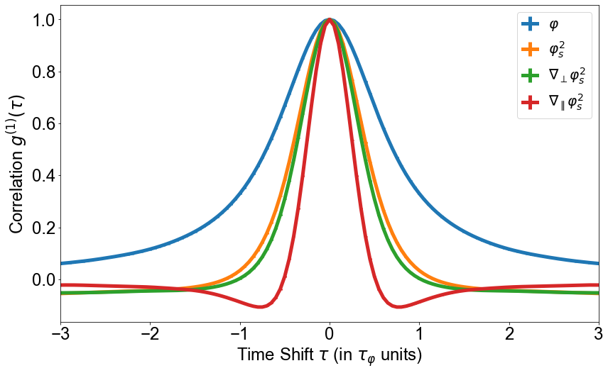
Figure 8: Auto-correlation of a simulated ALP dark matter field $\varphi$, the low-frequency component of its square $\varphi_{s}^{2}$ associated with stochastic fluctuations, and two gradient components perpendicular and parallel to $\boldsymbol{v}_{\mathrm{lab}}$: namely $\boldsymbol{\nabla}_{\perp}\varphi_{s}^{2}$ and $\boldsymbol{\nabla}_{\parallel}\varphi_{s}^{2}$, where the subscript $s$ denotes the low-frequency component associated with stochastic fluctuations.

IV.4.2 Signal model

Assuming the quadratic coupling Hamiltonian [Eq. (9)], the pseudo-magnetic field is given by $\boldsymbol{\Upsilon}_{q}=\boldsymbol{\nabla}\varphi^{2}$ and the signal observed in a GNOME sensor is $\propto\hat{\boldsymbol{m}}\cdot\boldsymbol{\Upsilon}_{q}$. As the detectors have limited bandwidth $\Delta\omega$, for the case where $\Delta\omega\ll\omega_{c}$ the fast oscillations at $2\omega_{c}$ are not observable in the measurement. The measured pseudo-magnetic field can be approximated by the near-dc component

$$\boldsymbol{\Upsilon}_{q}=\boldsymbol{\nabla}\varphi^{2}\approx\frac{A^{2}}{2N}\sum_{n,m=1}^{N}\boldsymbol{k}_{nm}\sin(\omega_{nm}t-\boldsymbol{k}_{nm}\cdot\boldsymbol{r}+\theta_{nm}),$$ (29)

where $\omega_{nm}=\omega_{n}-\omega_{m}$, $\boldsymbol{k}_{nm}=\boldsymbol{k}_{n}-\boldsymbol{k}_{m}$, and $\theta_{nm}=\theta_{n}-\theta_{m}$. Such a signal can be well characterized by two parameters: coherence time and amplitude.

For a solitary magnetometer or comagnetometer, a UBDM signature would be difficult to distinguish from comparably large background noise. Our strategy for analysis of GNOME data, presently underway, is to measure the cross-correlation between data measured at different stations. For stations with aligned sensitive axes and separations $\lesssim\lambda{{}_{\mbox{\scriptsize coh}}}$ and time delays $\lesssim\tau{{}_{\mbox{\scriptsize coh}}}$, UBDM quadratically coupled to atomic spins could generate a common-mode signal that might be distinguishable from uncorrelated background noise for sufficiently strong interactions. Figure 8 shows the auto-correlation function of simulated ALP signals, which is equivalent to the cross-correlation between stations with aligned sensitive axes within a coherence patch (ignoring any contribution from uncorrelated noise). The width of the correlation feature is $\approx\tau{{}_{\mbox{\scriptsize coh}}}$ in relative time shift units. This technique of intensity interferometry will enable a search for the quadratic coupling to ALPs over a mass range $\sim 10^{-14}$ eV – $10^{-9}$ eV using GNOME [63].

IV.5 Solar axion halo

Another theoretical possibility, closely related to the axion star model described in Sec. IV.2, is that tidal shearing forces may enable astrophysical bodies such as Earth and the Sun to capture UBDM in their gravitational fields and form a local halo [140, 141, 142, 143, 144], see Fig. 9. In these models, the Earth or Sun effectively acts as a seed in the formation process of the axion star. If such a process occurs, there would be a substantial overdensity of the ALP field near these bodies as compared to the average dark matter density as discussed in Refs. [140, 142]. Possible mechanisms for capture of dark matter by dense astrophysical bodies have been studied, for example, in Refs. [145, 146, 147, 148, 149, 150], and continue to be actively investigated.

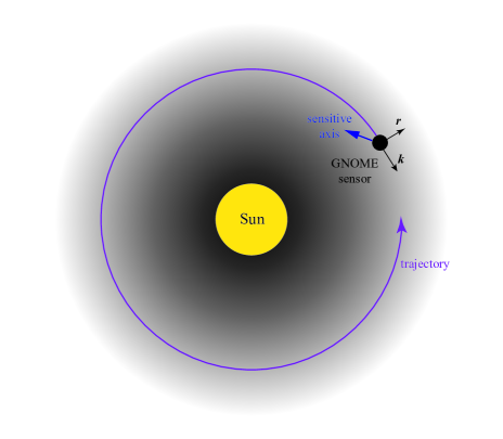
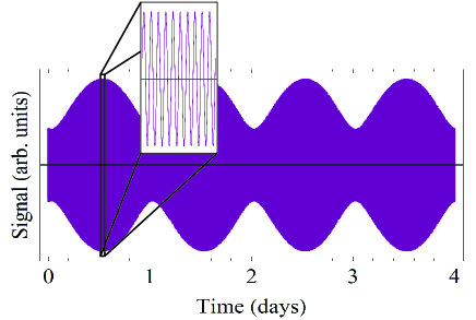
Figure 9: Upper diagram: Schematic diagram of Earth moving through a solar ALP halo. The pseudo-magnetic field associated with a solar ALP halo coupling to atomic spins has both a radial component in the $-\hat{\boldsymbol{r}}$ direction due to the spatial gradient and a transverse component due to the “ALP wind” directed along the ALP halo’s relative velocity with respect to the lab frame, $\hat{\boldsymbol{k}}$. Lower plot: example signal due to the linear spin coupling. Signal is shown over four days, exhibiting an envelope function due to the daily modulation of the signal due to the rotation of the GNOME sensor’s sensitive axis with respect to the pseudo-magnetic field $\boldsymbol{\Upsilon}$. Inset shows the fast oscillation at the Compton frequency.

IV.5.1 Theoretical description

Here we assume the model of a gravitationally bound solar ALP halo described in Refs. [140, 142], and also assume that the halo is non-rotating (i.e., at rest with respect to the Sun). For a solar halo, the ALP field amplitude at the position of Earth exponentially decays over a characteristic length scale given by

$$R_{\star}\approx\frac{\hbar^{2}}{G_{N}M_{\odot}m_{a}^{2}}\,,$$ (30)

where $G_{N}$ is Newton’s gravitational constant and $M_{\odot}$ is the Sun’s mass. For the solar ALP halo to extend to the position of Earth, we require $R_{\star}\gtrsim 1\,\textrm{AU}$. This imposes the requirement that $m_{a}c^{2}\lesssim 10^{-14}~{}{\rm eV}$. The ALP field oscillates at $\approx\omega_{c}$ with a coherence time $\tau{{}_{\mbox{\scriptsize coh}}}\gtrsim m_{a}R_{\star}^{2}/\hbar$. For $m_{a}c^{2}\lesssim 10^{-14}~{}{\rm eV}$, the coherence time is longer than $\sim 10^{7}$ s; therefore, we can treat oscillations of the ALP field as effectively single frequency (i.e., monochromatic). Thus the ALP field can be described as [140, 142]:

$$\varphi(\boldsymbol{r},t)\approx\varphi_{0}\cos{\left(\omega_{c}t-\boldsymbol{k}\cdot\boldsymbol{r}+\theta\right)}e^{-r/R_{\star}}\,,$$ (31)

where $\varphi_{0}$ is a constant determined by the overall energy density in the solar ALP halo and $\theta$ is a random phase, constant over the coherence time and coherence length. For simplicity, in this example we set $\theta=0$.

IV.5.2 Signal model

The exotic pseudo-magnetic field due to a solar ALP halo for the linear spin interaction is given by

$$\boldsymbol{\Upsilon}_{l}=\boldsymbol{\nabla}\varphi(\boldsymbol{r},t)=\varphi_{0}e^{-r/R_{\star}}{\left[\boldsymbol{k}\sin{\left(\omega_{c}t-\boldsymbol{k}\cdot\boldsymbol{r}\right)}-\frac{\hat{\boldsymbol{r}}}{R_{\star}}\cos{\left(\omega_{c}t-\boldsymbol{k}\cdot\boldsymbol{r}\right)}\right]}\,,$$ (32)

and for the quadratic spin interaction is given by

$$\boldsymbol{\Upsilon}_{q}=\boldsymbol{\nabla}\varphi^{2}(\boldsymbol{r},t)=\varphi_{0}^{2}e^{-2r/R_{\star}}{\left[\boldsymbol{k}\sin{\left(2\omega_{c}t-2\boldsymbol{k}\cdot\boldsymbol{r}\right)}-\frac{2\hat{\boldsymbol{r}}}{R_{\star}}\cos^{2}{\left(\omega_{c}t-\boldsymbol{k}\cdot\boldsymbol{r}\right)}\right]}~{}.$$ (33)

We note that in both cases there are two components of $\boldsymbol{\Upsilon}$ in the lab frame [142]: (1) a radial component from the spatial ALP gradient directed toward the Sun’s position and (2) a transverse component along $\boldsymbol{k}$ due to the ALP wind interaction [6, 5]. Because the relative velocity of Earth with respect to the Sun is dominated by its orbital motion ($\sim 100$ times faster than the velocity component due to Earth’s rotation about its axis), it turns out that all GNOME sensors have approximately the same $\boldsymbol{k}$ and thus see the same field. The amplitudes of the radial and transverse components of $\boldsymbol{\Upsilon}$ are relatively constant in time, so the signal observed in a particular GNOME sensor has a predictable daily modulation due to the time dependence of $\hat{\boldsymbol{r}}\cdot\hat{\boldsymbol{m}}$ and $\hat{\boldsymbol{k}}\cdot\hat{\boldsymbol{m}}$ caused by the rotation of Earth. An example of the time dependence of such a signal is shown in the lower plot of Fig. 9.

Analysis of GNOME data to search for a solar ALP halo is in progress. The strategy is to search for a persistent single-frequency signal in cross-correlation data between stations, and then use the predicted daily modulation to distinguish between a signal from a solar ALP halo and systematic backgrounds.

IV.6 Exotic Low-mass Fields (ELFs) emitted from black hole mergers

In Ref. [56], a subset of the present authors considered a possibility that bursts of ultrarelativistic scalar fields can be produced in the course of some high energy astrophysical event such as a supernova explosion, a binary black hole merger, or in conjunction with a fast radio burst via some as yet unknown coherent process (see, for example, Ref. [152]). These “exotic low-mass fields” (ELFs) would thus have large mode occupation numbers, enabling their treatment as classical waves with oscillation frequency given by $\hbar\omega=\sqrt{m^{2}c^{4}+p^{2}c^{2}}\approx pc$. Such ELFs can be searched for with GNOME.

IV.6.1 Theoretical description

Consider a scenario where some energy $\Delta E$ is radiated isotropically in the form of a Gaussian ELF burst with duration $\tau_{0}$ at the source. The Klein-Gordon equation for $\varphi(r)$ can be solved to obtain

$$\varphi(t)\approx \frac{A_{0}}{R}\sqrt{\frac{\tau_{0}}{\tau}}\exp{\left(-\frac{(t-t_{s})^{2}}{2\tau^{2}}\right)}$$

$$\times\cos{\left(\omega_{0}(t-t_{s})-\frac{\omega_{0}}{4\delta t}(t-t_{s})^{2}\right)}\,,$$ (34)

where $\omega_{0}$ is the central frequency of the wave packet, $\tau$ the duration of the pulse as measured by sensors on Earth, $t_{s}=R/v_{g}$ represents the transit time of the ELF pulse from a source at distance $R$ from Earth, and $v_{g}$ the group velocity. The delay time between an electromagnetic or gravitational wave trigger and an ELF pulse is $\delta t=R/v_{g}-R/c$. In terms of the total energy released, the amplitude $A_{0}$ is given by

$$A_{0}\approx\frac{1}{\pi^{1/4}}{\left(\frac{1}{\omega_{0}}\sqrt{\frac{c\Delta E}{2\pi\tau_{0}}}\right)}\,.$$ (35)

Equations (34) and (35) describe a Gaussian wavepacket which disperses with a chirp rate

$$\frac{d\omega(t)}{dt}=-\frac{1}{\tau_{0}\tau}=-\frac{\omega_{0}}{2\delta t}\,.$$ (36)

Notably, the chirp rate is constrained by the central frequency and the delay from the electromagnetic or gravitational wave trigger.

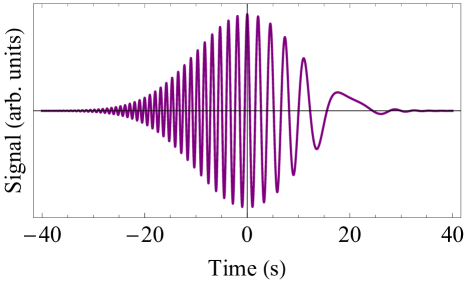
Figure 10: Example signal of an ELF measured by a GNOME sensor based on Eq. (34), with $\omega_{0}=2\pi\times(0.5~{}{\rm Hz})$, $\tau=10$ s, and $\delta t=10$ s.

IV.6.2 Signal model

As a consequence of the couplings described in Eqs. (3) to (9), the existence of scalar fields with a form such as that described by Eq. (34) would lead to pseudo-magnetic fields in GNOME due to interaction terms proportional to $\boldsymbol{S}\cdot\boldsymbol{\nabla}\varphi(\boldsymbol{r},t)$ and $\boldsymbol{S}\cdot\boldsymbol{\nabla}[\varphi(\boldsymbol{r},t)]^{2}$. A signal due to an ELF event (Fig. 10) would therefore: (1) originate from the same source as the electromagnetic or gravitational wave trigger; (2) have a spatial pattern in the GNOME network given by the projection of the ELF velocity vector on the axes of the sensors in the network; and (3) have a characteristic chirp pattern given by Eq. (36). Using these characteristics, we have designed an analysis algorithm to search for ELF signals in GNOME data. Measurements from the GNOME sensors are projected into the time-frequency plane with a resolution chosen to match the expected signal dispersion. We then construct a network-wide test statistic and search for signals consistent with ELFs in the GNOME data in intervals of time shortly after reported binary black hole merger and fast radio burst events.

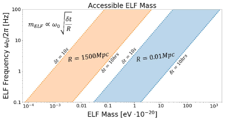
Figure 11: Accessible masses for ELFs from sources located at distances R = 1500 Mpc and R = 0.01 Mpc. The left and right edges of the bands are set by the delay times $10\,\rm{s}<\delta t<10\,\rm{hr}$.

We show in Fig. 11 the range of masses that are accessible by GNOME given the bandwidth of the magnetometers, assuming an observation time of 10 hours after the trigger. Thus GNOME can act as a “telescope” to detect ELF signals from sources that generate ALP bursts of sufficient intensity.

IV.7 Other potential candidates

There are many other exotic physics scenarios that can potentially be searched for using data from the GNOME experiment, demonstrating the versatility of the general approach. For example, as already noted, it may be that there are relatively strong interactions between particles in the dark sector. Such interactions could cause dark matter particles to coalesce into large composite “blobs” [33]. In contrast to the axion star, Q-ball, and solar axion-halo scenarios already considered above, which are composite states of ultralight particles, there could be dark matter blobs formed from heavy fermions or bosons that exert long-range forces mediated by other fundamental constituents of the dark sector [33, 153]. Other possible search targets for the GNOME experiment are ALP waves emanating from black hole superradiance [154] or from the collapse of axion stars [152]. In related work, unshielded magnetometer networks have been used to search for signals from dark (or hidden) photons [155, 156] and axions [157].

Yet another possible search target for GNOME are UBDM streams, in particular those gravitationally focused by other bodies in the solar system. Cosmological simulations indicate that up to $10^{12}$ small-velocity-dispersion (compared to that in the SHM) streams of DM may be present in the vicinity of the solar system [158]. The deflection experienced by these particles depends on the mass distribution of the source of gravitational focusing, is independent of the DM particle mass, and is inversely proportional to the square of its velocity. For UBDM, its wave nature has to be considered for a full description of the spectral signatures due to gravitational focusing [159] Generally, for deflection of particles by the gravitational potential of the Earth, efficient focusing on Earth’s surface (where GNOME operates) occurs for particles with velocities of approximately 10 to 20 km/s [160, 161]. In this case, flux enhancements of up to $10^{9}$ are predicted. Gravitational deflection by other objects in the solar system, such as Jupiter, can also generate flux enhancements on Earth. This requires larger stream velocities of approximately $10^{-3}$ c and results in smaller enhancements of only $10^{6}$ [162]. Again, the networked approach of GNOME offers several advantages when searching for such gravitationally focused streams. Namely, the small size of such stream foci, on the order of a few km for deflection in Earth’s gravitational potential and much less for that of Jupiter, leads to transient signals lasting only about 10 s. This can be difficult to distinguish from noise when only a single detector is employed. For long streams, there is a chance of the detecting the enhanced DM flux daily with one or more detectors over the course of several weeks. Obviously, the likelihood of encountering the high flux regions increases with the number of sensors in a network. A network also allows for precisely determining the spatial direction of the stream, which can help to better understand the origins of such streams when detected, although this can be a complex endeavor as upstream sources of gravitational deflection also have to be considered. Furthermore, sensors at approximately the same latitudes could produce correlated signals from the same focused-DM source (Fig.  12). The geographical locations of GNOME sensors make it viable for such correlations.

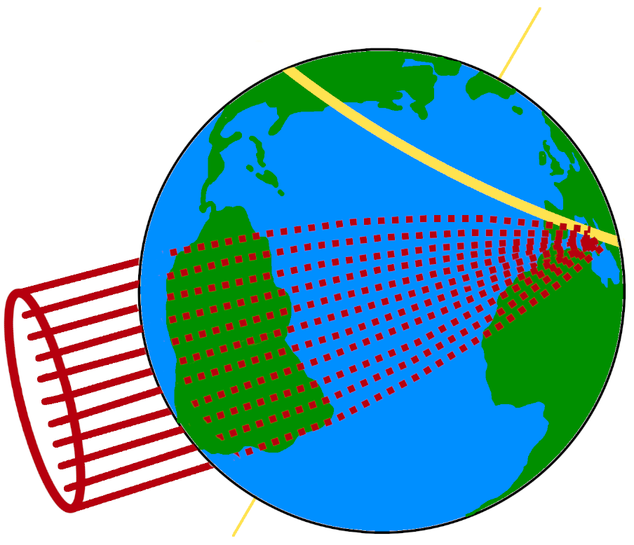
Figure 12: Example of a low velocity UBDM stream (red) gravitationally focused into a small region on Earth’s surface, the trajectories are approximately following predictions made in Ref. [160]. As Earth rotates around its axis, the focus follows a path (yellow) along a fixed latitude.

While GNOME is primarily a tool for detection of transient “new-physics” signals, its sister experiment, the Cosmic Axion Spin-Precession Experiment (CASPEr) [9, 11, 16], is searching for oscillating (but not necessarily transient) effects of galactic dark matter and dark matter concentrated in the Sun- and Earth-bound halos. CASPEr operates simultaneously in two locations, Boston University (USA) and the Helmholtz Institute, Johannes Gutenberg University, Mainz (Germany). The central idea of CASPEr is that it is a nuclear magnetic resonance (NMR) experiment, where the role of the transverse oscillating magnetic field “$\boldsymbol{B}_{1}$” is relegated to the ambient Axion/ALP field either through its coupling to gluons (CASPEr-electric) or via its gradient interactions [see Eqs. (6) and (9); CASPEr-gradient]. While CASPEr will reach up to Compton frequencies $\approx$600 MHz, it has already ventured into the much lower-frequency range [12, 13], from near DC to several hertz. The low-frequency range has also been explored by various other experiments [10, 17, 18, 26, 20].

The Advanced-GNOME comagnetometers [32, 84] are ideally suited to contribute to “CASPEr-like” searches in the Compton frequency range from near-DC to several hundred hertz, with the sensitivity that is estimated to be competitive to the best previous searches. The results of the first experiments in this direction may be expected already at the early stages of Advanced GNOME, as a search in this mode does not require the full network capabilities. However, as with GNOME, we expect that the network will be immediately useful in vetoing spurious signals from various laboratory inferences, which will likely be different in different laboratories. Moreover, the network offers interesting possibilities of correlating the stochastic behavior of the signal in different stations that may offer an additional tool for discriminating the new-physics signals.

V Conclusion and outlook

The idea of GNOME is to carry out synchronous measurements using optical atomic magnetometers and comagnetometers operating within magnetically shielded environments in distant locations. The GNOME experiment searches for a class of signals different from that probed by most other experiments, namely transient and stochastic effects that could arise from ALP fields of astrophysical origin passing through Earth during a finite time. By analyzing the correlation between the signals from multiple, geographically separated sensors, it is possible to probe a wide variety of exotic physics scenarios.

When the idea of GNOME was conceived, ALP domain walls were the sole targets of the search [31, 28]. As the collaboration expanded and matured, we gradually realized that there are many more interesting physics scenarios that can be investigated with this tool, as, we hope, we have been able to convince the reader of this “GNOME science-case” article. Extrapolating from the first 10 years of the GNOME collaboration’s work, we may only expect the science case to continue its expansion, hopefully leading to a discovery of “new” physics.

The advent of GNOME was soon followed by the establishment of networks of atomic clocks [89] introduced to search for scalar UBDM whose effect is to produce apparent oscillation of fundamental constants, rather than causing spin precession. At the same time, it was realized that certain UBDM candidates like the relaxion [163, 164] may have mixed intrinsic parity and displaying both the scalar and pseudoscalar properties. This provides a motivation for building hybrid-sensor networks (for example, (co)magnetometer-clock networks) to cross-correlate the signals and enhance the background-suppression capabilities. We expect this cross-network approach to become commonplace in future work. Moreover, GNOME is planning future science runs to be synchronized with gravitational-wave detector networks such as LIGO/VIRGO in order to carry out “exotic” multimessenger astronomy [56].

It appears that the science case for search networks such as GNOME is mostly limited by our current scientific horizons and there are, in fact, many other interesting and unexpected signals we could be looking for, had we better imagination. But could we perhaps look for such signals before we realize what they are? It appears that modern machine-learning approaches indeed offer us such an exciting opportunity. It might work along the following lines: a machine-learning system is trained on the data from GNOME (and/or an expanded hybrid-sensor network) and establishes the “normal” dynamic state of the network. It is then further trained on a variety of new-physics scenarios. As a result of the training that can continue for the lifetime of the experiment, the artificial intelligence (AI) system would be able to recognize unusual events or patterns on the network. While this may look like a remote prospect, one should recognize that the task at hand is not too different from that of detection of unidentified threats, which is routinely done at present by automated security systems.

In conclusion of our overview of the “GNOME science”, we mention that, apart from fundamental physics, magnetometer networks may also be useful in more “down-to-Earth” applications such as, for example, the study of magnetic signal patterns in urban environments and what they reveal about cities [165, 166].

References

- Jackson Kimball and van Bibber [2022] D. F. Jackson Kimball and K. van Bibber, The Search for Ultralight Bosonic Dark Matter (Springer, 2022).
- Graham et al. [2015a] P. W. Graham, I. G. Irastorza, S. K. Lamoreaux, A. Lindner, and K. A. van Bibber, Experimental searches for the axion and axion-like particles, Annu. Rev. Nucl. Part. Sci. 65, 485 (2015a).
- Graham et al. [2016] P. W. Graham, D. E. Kaplan, J. Mardon, S. Rajendran, and W. A. Terrano, Dark matter direct detection with accelerometers, Phys. Rev. D 93, 075029 (2016).
- Safronova et al. [2018] M. Safronova, D. Budker, D. DeMille, D. F. Jackson Kimball, A. Derevianko, and C. W. Clark, Search for new physics with atoms and molecules, Rev. Mod. Phys. 90, 025008 (2018).
- Stadnik and Flambaum [2014] Y. Stadnik and V. Flambaum, Axion-induced effects in atoms, molecules, and nuclei: Parity nonconservation, anapole moments, electric dipole moments, and spin-gravity and spin-axion momentum couplings, Phys. Rev. D 89, 043522 (2014).
- Graham et al. [2018] P. W. Graham, D. E. Kaplan, J. Mardon, S. Rajendran, W. A. Terrano, L. Trahms, and T. Wilkason, Spin precession experiments for light axionic dark matter, Phys. Rev. D 97, 055006 (2018).
- Budker and Jackson Kimball [2013] D. Budker and D. F. Jackson Kimball, Optical Magnetometry (Cambridge University Press, 2013).
- Budker and Romalis [2007] D. Budker and M. Romalis, Optical magnetometry, Nature Phys. 3, 227 (2007).
- Budker et al. [2014] D. Budker, P. W. Graham, M. Ledbetter, S. Rajendran, and A. O. Sushkov, Proposal for a cosmic axion spin precession experiment (casper), Phys. Rev. X 4, 021030 (2014).
- Abel et al. [2017] C. Abel, N. J. Ayres, G. Ban, G. Bison, K. Bodek, V. Bondar, M. Daum, M. Fairbairn, V. V. Flambaum, P. Geltenbort, et al., Search for axionlike dark matter through nuclear spin precession in electric and magnetic fields, Phys. Rev. X 7, 041034 (2017).
- Garcon et al. [2017] A. Garcon, D. Aybas, J. W. Blanchard, G. Centers, N. L. Figueroa, P. W. Graham, D. F. Jackson Kimball, S. Rajendran, M. G. Sendra, A. O. Sushkov, L. Trahms, T. Wang, A. Wickenbrock, T. Wu, and D. Budker, The Cosmic Axion Spin Precession Experiment (CASPEr): a dark-matter search with nuclear magnetic resonance, Quantum Sci. Technol. 3, 014008 (2017).
- Wu et al. [2019] T. Wu, J. W. Blanchard, G. P. Centers, N. L. Figueroa, A. Garcon, P. W. Graham, D. F. Jackson Kimball, S. Rajendran, Y. V. Stadnik, A. O. Sushkov, et al., Search for axionlike dark matter with a liquid-state nuclear spin comagnetometer, Phys. Rev. Lett. 122, 191302 (2019).
- Garcon et al. [2019] A. Garcon, J. W. Blanchard, G. P. Centers, N. L. Figueroa, P. W. Graham, D. F. Jackson Kimball, S. Rajendran, A. O. Sushkov, Y. V. Stadnik, A. Wickenbrock, et al., Constraints on bosonic dark matter from ultralow-field nuclear magnetic resonance, Science Advances 5, eaax4539 (2019).
- Aybas et al. [2021a] D. Aybas, H. Bekker, J. Blanchard, D. Budker, G. Centers, N. Figueroa, A. Gramolin, D. F. Jackson Kimball, A. Wickenbrock, and A. Sushkov, Quantum sensitivity limits of nuclear magnetic resonance experiments searching for new fundamental physics, Quantum Sci. Technol. 6, 034007 (2021a).
- Roussy et al. [2021] T. S. Roussy, D. A. Palken, W. B. Cairncross, B. M. Brubaker, D. N. Gresh, M. Grau, K. C. Cossel, K. B. Ng, Y. Shagam, Y. Zhou, et al., Experimental constraint on axionlike particles over seven orders of magnitude in mass, Phys. Rev. Lett. 126, 171301 (2021).
- Aybas et al. [2021b] D. Aybas, J. Adam, E. Blumenthal, A. V. Gramolin, D. Johnson, A. Kleyheeg, S. Afach, J. W. Blanchard, G. P. Centers, A. Garcon, M. Engler, N. L. Figueroa, M. G. Sendra, A. Wickenbrock, M. Lawson, T. Wang, T. Wu, H. Luo, H. Mani, P. Mauskopf, P. W. Graham, S. Rajendran, D. F. Jackson Kimball, D. Budker, and A. O. Sushkov, Search for axionlike dark matter using solid-state nuclear magnetic resonance, Phys. Rev. Lett. 126, 141802 (2021b).
- Jiang et al. [2021a] M. Jiang, H. Su, A. Garcon, X. Peng, and D. Budker, Search for axion-like dark matter with spin-based amplifiers, Nature Phys. 17, 1402 (2021a).
- Bloch et al. [2022] I. M. Bloch, G. Ronen, R. Shaham, O. Katz, T. Volansky, and O. Katz, New constraints on axion-like dark matter using a Floquet quantum detector, Sci. Adv. 8, eabl8919 (2022).
- Lee et al. [2022] J. Lee, M. Lisanti, W. A. Terrano, and M. Romalis, Laboratory Constraints on the Neutron-Spin Coupling of feV-scale Axions, arXiv:2209.03289 10.48550/arXiv.2209.03289 (2022).
- Abel et al. [2022] C. Abel, N. Ayres, G. Ban, G. Bison, K. Bodek, V. Bondar, E. Chanel, C. Crawford, M. Daum, B. Dechenaux, et al., Search for ultralight axion dark matter in a side-band analysis of a Hg-199 free-spin precession signal, arXiv:2212.02403 10.48550/arXiv.2212.02403 (2022).
- Freese et al. [2013] K. Freese, M. Lisanti, and C. Savage, Colloquium: Annual modulation of dark matter, Rev. Mod. Phys. 85, 1561 (2013).
- Pillepich et al. [2014] A. Pillepich, M. Kuhlen, J. Guedes, and P. Madau, The distribution of dark matter in the Milky Way’s disk, Astrophys. J. 784, 161 (2014).
- Evans et al. [2019] N. W. Evans, C. A. O’Hare, and C. McCabe, Refinement of the standard halo model for dark matter searches in light of the gaia sausage, Phys. Rev. D 99, 023012 (2019).
- Foster et al. [2018] J. W. Foster, N. L. Rodd, and B. R. Safdi, Revealing the dark matter halo with axion direct detection, Phys. Rev. D 97, 123006 (2018).
- Centers et al. [2021] G. P. Centers, J. W. Blanchard, J. Conrad, N. L. Figueroa, A. Garcon, A. V. Gramolin, D. F. Jackson Kimball, M. Lawson, B. Pelssers, J. A. Smiga, et al., Stochastic fluctuations of bosonic dark matter, Nature Comm. 12, 7321 (2021).
- Lisanti et al. [2021] M. Lisanti, M. Moschella, and W. Terrano, Stochastic properties of ultralight scalar field gradients, Phys. Rev. D 104, 055037 (2021).
- Gramolin et al. [2022] A. V. Gramolin, A. Wickenbrock, D. Aybas, H. Bekker, D. Budker, G. P. Centers, N. L. Figueroa, D. F. Jackson Kimball, and A. O. Sushkov, Spectral signatures of axionlike dark matter, Phys. Rev. D 105, 035029 (2022).
- Pustelny et al. [2013] S. Pustelny, D. F. Jackson Kimball, C. Pankow, M. P. Ledbetter, P. Wlodarczyk, P. Wcislo, M. Pospelov, J. R. Smith, J. Read, W. Gawlik, et al., The global network of optical magnetometers for exotic physics (gnome): A novel scheme to search for physics beyond the standard model, Annalen der Physik 525, 659 (2013).
- Afach et al. [2018] S. Afach, D. Budker, G. DeCamp, V. Dumont, Z. D. Grujić, H. Guo, D. Jackson Kimball, T. Kornack, V. Lebedev, W. Li, et al., Characterization of the global network of optical magnetometers to search for exotic physics (gnome), Phys. Dark Universe 22, 162 (2018).
- Afach et al. [2021] S. Afach, B. C. Buchler, D. Budker, C. Dailey, A. Derevianko, V. Dumont, N. L. Figueroa, I. Gerhardt, Z. D. Grujić, H. Guo, et al., Search for topological defect dark matter with a global network of optical magnetometers, Nature Phys. 17, 1396 (2021).
- Pospelov et al. [2013] M. Pospelov, S. Pustelny, M. P. Ledbetter, D. F. Jackson Kimball, W. Gawlik, and D. Budker, Detecting domain walls of axionlike models using terrestrial experiments, Phys. Rev. Lett. 110, 021803 (2013).
- Padniuk et al. [2022] M. Padniuk, M. Kopciuch, R. Cipolletti, A. Wickenbrock, D. Budker, and S. Pustelny, Response of atomic spin-based sensors to magnetic and nonmagnetic perturbations, Scientific Reports 12, 324 (2022).
- Grabowska et al. [2018] D. M. Grabowska, T. Melia, and S. Rajendran, Detecting dark blobs, Phys. Rev. D 98, 115020 (2018).
- Yashchuk et al. [2011] V. Yashchuk, S. Lee, and E. Paperno, Magnetic shielding, in Optical Magnetometry (Cambridge University Press, 2011) pp. 225–248.
- Jackson Kimball et al. [2016] D. Jackson Kimball, J. Dudley, Y. Li, S. Thulasi, S. Pustelny, D. Budker, and M. Zolotorev, Magnetic shielding and exotic spin-dependent interactions, Phys. Rev. D 94, 082005 (2016).
- Jackson Kimball [2015] D. F. Jackson Kimball, Nuclear spin content and constraints on exotic spin-dependent couplings, New J. Phys. 17, 073008 (2015).
- Stadnik and Flambaum [2015] Y. Stadnik and V. Flambaum, Nuclear spin-dependent interactions: searches for wimp, axion and topological defect dark matter, and tests of fundamental symmetries, Eur. Phys. J. C 75, 1 (2015).
- Peccei and Quinn [1977a] R. Peccei and H. Quinn, CP conservation in the presence of pseudoparticles, Phys. Rev. Lett. 38, 1440 (1977a).
- Peccei and Quinn [1977b] R. Peccei and H. Quinn, Constraints imposed by CP conservation in the presence of pseudoparticles, Phys. Rev. D 16, 1791 (1977b).
- Weinberg [1978] S. Weinberg, A new light boson?, Phys. Rev. Lett. 40, 223 (1978).
- Wilczek [1978] F. Wilczek, Problem of strong and invariance in the presence of instantons, Phys. Rev. Lett. 40, 279 (1978).
- Graham et al. [2015b] P. W. Graham, D. E. Kaplan, and S. Rajendran, Cosmological Relaxation of the Electroweak Scale, Phys. Rev. Lett. 115, 221801 (2015b).
- Co et al. [2021] R. T. Co, L. J. Hall, and K. Harigaya, Predictions for axion couplings from ALP cogenesis, J. High Energy Phys. 2021, 172.
- Svrcek and Witten [2006] P. Svrcek and E. Witten, Axions in string theory, J. High Energy Phys. 06, 051.
- Arvanitaki et al. [2010] A. Arvanitaki, S. Dimopoulos, S. Dubovsky, N. Kaloper, and J. March-Russell, String axiverse, Phys. Rev. D 81, 123530 (2010).
- Abbott and Sikivie [1983] L. F. Abbott and P. Sikivie, A cosmological bound on the invisible axion, Physics Letters B 120, 133 (1983).
- Preskill et al. [1983] J. Preskill, M. B. Wise, and F. Wilczek, Cosmology of the invisible axion, Physics Letters B 120, 127 (1983).
- Dine and Fischler [1983] M. Dine and W. Fischler, The not-so-harmless axion, Physics Letters B 120, 137 (1983).
- Freivogel [2010] B. Freivogel, Anthropic explanation of the dark matter abundance, Journal of Cosmology and Astroparticle Physics 2010, 021.
- Chang et al. [1998] S. Chang, C. Hagmann, and P. Sikivie, Studies of the motion and decay of axion walls bounded by strings, Phys. Rev. D 59, 023505 (1998).
- Arkani-Hamed et al. [2009] N. Arkani-Hamed, D. P. Finkbeiner, T. R. Slatyer, and N. Weiner, A theory of dark matter, Phys. Rev. D 79, 015014 (2009).
- Arias et al. [2012] P. Arias, D. Cadamuro, M. Goodsell, J. Jaeckel, J. Redondo, and A. Ringwald, WISPy cold dark matter, J. Cosm. Astropart. Phys. 2012, 013 (2012).
- Graham and Scherlis [2018] P. W. Graham and A. Scherlis, Stochastic axion scenario, Phys. Rev. D 98, 035017 (2018).
- Duffy and Van Bibber [2009] L. D. Duffy and K. Van Bibber, Axions as dark matter particles, New J. Phys. 11, 105008 (2009).
- Graham and Rajendran [2013] P. W. Graham and S. Rajendran, New observables for direct detection of axion dark matter, Phys. Rev. D 88, 035023 (2013).
- Dailey et al. [2021] C. Dailey, C. Bradley, D. F. Jackson Kimball, I. A. Sulai, S. Pustelny, A. Wickenbrock, and A. Derevianko, Quantum sensor networks as exotic field telescopes for multi-messenger astronomy, Nature Astron. 5, 150 (2021).
- [57] V. V. Flambaum, Axioelectric effect and other manifestations of dark matter and dark energy in laboratory experiments, Proceedings of the 9th Patras Workshop on Axions, WIMPs and WISPs, Mainz, Germany, 2013, https://axion-wimp2013.desy.de/e201031/index_eng.html.
- Jackson Kimball et al. [2020] D. F. Jackson Kimball, S. Afach, D. Aybas, J. Blanchard, D. Budker, G. Centers, M. Engler, N. Figueroa, A. Garcon, P. Graham, et al., Overview of the cosmic axion spin precession experiment (CASPEr), in Microwave Cavities and Detectors for Axion Research, edited by G. Carosi, G. Rybka, and K. van Bibber (Springer, 2020) pp. 105–121.
- Olive and Pospelov [2008] K. A. Olive and M. Pospelov, Environmental dependence of masses and coupling constants, Phys. Rev. D 77, 043524 (2008).
- Damour and Nordtvedt [1993a] T. Damour and K. Nordtvedt, General relativity as a cosmological attractor of tensor-scalar theories, Phys. Rev. Lett. 70, 2217 (1993a).
- Damour and Nordtvedt [1993b] T. Damour and K. Nordtvedt, Tensor-scalar cosmological models and their relaxation toward general relativity, Phys. Rev. D 48, 3436 (1993b).
- Damour and Polyakov [1994] T. Damour and A. M. Polyakov, The string dilation and a least coupling principle, Nucl. Phys. B 423, 532 (1994).
- Masia-Roig et al. [2022] H. Masia-Roig, N. L. Figueroa, A. Bordon, J. A. Smiga, D. Budker, G. P. Centers, A. V. Gramolin, P. S. Hamilton, S. Khamis, C. A. Palm, et al., Intensity interferometry for ultralight bosonic dark matter detection, arXiv:2202.02645 10.48550/arXiv.2202.02645 (2022).
- Bernreuther [2002] W. Bernreuther, Cp violation and baryogenesis, in CP Violation in Particle, Nuclear and Astrophysics, edited by M. Beyer (Springer Berlin Heidelberg, Berlin, Heidelberg, 2002) pp. 237–293.
- Włodarczyk et al. [2014] P. Włodarczyk, S. Pustelny, D. Budker, and M. Lipiński, Multi-channel data acquisition system with absolute time synchronization, Nucl. Instrum. Methods. Phys. Res. A 763, 150 (2014).
- Kominis et al. [2003] I. Kominis, T. Kornack, J. Allred, and M. Romalis, A subfemtotesla multichannel atomic magnetometer, Nature 422, 596–599 (2003).
- Groeger et al. [2006] S. Groeger, G. Bison, J. L. Schenker, R. Wynands, and A. Weis, A high-sensitivity laser-pumped Mx magnetometer, Eur. Phys. J. D 38, 239–247 (2006).
- Pustelny et al. [2008] S. Pustelny, A. Wojciechowski, M. Gring, J. Kotyrba, M. amd Zachorowski, and G. W., Magnetometry based on nonlinear magneto-optical rotation with amplitude-modulated light, J. Appl. Phys. 103, 063108 (2008).
- Kornack and Romalis [2002] T. W. Kornack and M. V. Romalis, Dynamics of two overlapping spin ensembles interacting by spin exchange, Phys. Rev. Lett. 89, 253002 (2002).
- Terrano and Romalis [2021] W. A. Terrano and M. V. Romalis, Comagnetometer probes of dark matter and new physics, Quantum Science and Technology 7, 014001 (2021).
- Masia-Roig et al. [2020] H. Masia-Roig, J. A. Smiga, D. Budker, V. Dumont, Z. Grujic, D. Kim, D. F. Jackson Kimball, V. Lebedev, M. Monroy, S. Pustelny, et al., Analysis method for detecting topological defect dark matter with a global magnetometer network, Phys. Dark Universe 28, 100494 (2020).
- Smiga [2022] J. A. Smiga, Assessing the quality of a network of vector-field sensors, Eur. Phys. J. D 76, 4 (2022).
- Jiang et al. [2022] M. Jiang, Y. Qin, X. Wang, Y. Wang, H. Su, X. Peng, and D. Budker, Floquet spin amplification, Phys. Rev. Lett. 128, 233201 (2022).
- Glenday et al. [2008] A. G. Glenday, C. E. Cramer, D. F. Phillips, and R. L. Walsworth, Limits on anomalous spin-spin couplings between neutrons, Phys. Rev. Lett. 101, 261801 (2008).
- Jiang et al. [2021b] M. Jiang, H. Su, Z. Wu, X. Peng, and D. Budker, Floquet maser, Sci. Adv. 7, eabe0719 (2021b).
- Venema et al. [1992] B. J. Venema, P. K. Majumder, S. K. Lamoreaux, B. R. Heckel, and E. N. Fortson, Search for a Coupling of Earth’s Gravitational Field to Nuclear Spins in Atomic Mercury, Phys. Rev. Lett. 68, 135 (1992).
- Feng et al. [2022] Y. Feng, D. Ning, S. Zhang, Z. Lu, and D. Sheng, Search for monopole-dipole interactions at the sub-millimeter range with a 129Xe-131Xe-Rb comagnetometer, Phys. Rev. Lett. 128, 231803 (2022).
- Jackson Kimball et al. [2013] D. F. Jackson Kimball, I. Lacey, J. Valdez, J. Swiatlowski, C. Rios, R. Peregrina-Ramirez, C. Montcrieffe, J. Kremer, J. Dudley, and C. Sanchez, A dual-isotope rubidium comagnetometer to search for anomalous long-range spin-mass (spin-gravity) couplings of the proton, Annalen der Physik 525, 514 (2013).
- Jackson Kimball et al. [2017] D. F. Jackson Kimball, J. Dudley, Y. Li, D. Patel, and J. Valdez, Constraints on long-range spin-gravity and monopole-dipole couplings of the proton, Phys. Rev. D 96, 075004 (2017).
- Jackson Kimball et al. [2023] D. F. Jackson Kimball, J. Dudley, Y. Li, D. Patel, and J. Valdez, Erratum: Constraints on long-range spin-gravity and monopole-dipole couplings of the proton [Phys. Rev. D 96, 075004 (2017)], Phys. Rev. D 107, 019903(E) (2023).
- Wang et al. [2020] Z. Wang, X. Peng, R. Zhang, H. Luo, J. Li, Z. Xiong, S. Wang, and H. Guo, Single-species atomic comagnetometer based on rb 87 atoms, Phys. Rev. Lett. 124, 193002 (2020).
- Ledbetter et al. [2012] M. Ledbetter, S. Pustelny, D. Budker, M. V. Romalis, J. Blanchard, and A. Pines, Liquid-state nuclear spin comagnetometers, Phys. Rev. Lett. 108, 243001 (2012).
- Wu et al. [2018] T. Wu, J. W. Blanchard, D. F. Jackson Kimball, M. Jiang, and D. Budker, Nuclear-spin comagnetometer based on a liquid of identical molecules, Phys. Rev. Lett. 121, 023202 (2018).
- Klinger et al. [2022] E. Klinger, T. Liu, M. Padniuk, M. Engler, T. Kornack, S. Pustelny, D. F. Jackson Kimball, D. Budker, and A. Wickenbrock, Polarization dynamics in a nuclear spin gyroscope, arXiv:2210.07687 10.48550/arXiv.2210.07687 (2022).
- Sikivie [1982] P. Sikivie, Axions, domain walls, and the early universe, Phys. Rev. Lett. 48, 1156 (1982).
- Kawasaki et al. [2015] M. Kawasaki, K. Saikawa, and T. Sekiguchi, Axion dark matter from topological defects, Phys. Rev. D 91, 065014 (2015).
- Vilenkin and Everett [1982] A. Vilenkin and A. E. Everett, Cosmic strings and domain walls in models with goldstone and pseudo-goldstone bosons, Phys. Rev. Lett. 48, 1867 (1982).
- Nagasawa and Kawasaki [1994] M. Nagasawa and M. Kawasaki, Collapse of axionic domain wall and axion emission, Phys. Rev. D 50, 4821 (1994).
- Derevianko and Pospelov [2014] A. Derevianko and M. Pospelov, Hunting for topological dark matter with atomic clocks, Nature Physics 10, 933 (2014).
- Zeldovich et al. [1974] Y. B. Zeldovich, I. Y. Kobzarev, and L. B. Okun, Cosmological Consequences of the Spontaneous Breakdown of Discrete Symmetry, Zh. Eksp. Teor. Fiz. 67, 3 (1974).
- Kim et al. [2022] D. Kim, D. F. Jackson Kimball, H. Masia-Roig, J. A. Smiga, A. Wickenbrock, D. Budker, Y. Kim, Y. C. Shin, and Y. K. Semertzidis, A machine learning algorithm for direct detection of axion-like particle domain walls, Phys. Dark Universe 37, 101118 (2022).
- Braaten and Zhang [2019] E. Braaten and H. Zhang, Colloquium: The physics of axion stars, Rev. Mod. Phys. 91, 041002 (2019).
- Eby et al. [2019] J. Eby, M. Leembruggen, L. Street, P. Suranyi, and L. Wijewardhana, Global view of QCD axion stars, Phys. Rev. D 100, 063002 (2019).
- Eby et al. [2021] J. Eby, L. Street, P. Suranyi, and L. Wijewardhana, Global view of axion stars with nearly Planck-scale decay constants, Phys. Rev. D 103, 063043 (2021).
- Eby et al. [2018a] J. Eby, M. Leembruggen, L. Street, P. Suranyi, and L. Wijewardhana, Approximation methods in the study of boson stars, Phys. Rev. D 98, 123013 (2018a).
- Chavanis [2011] P.-H. Chavanis, Mass-radius relation of Newtonian self-gravitating Bose-Einstein condensates with short-range interactions. I. Analytical results, Phys. Rev. D 84, 043531 (2011).
- Chavanis and Delfini [2011] P.-H. Chavanis and L. Delfini, Mass-radius relation of newtonian self-gravitating bose-einstein condensates with short-range interactions. ii. numerical results, Phys. Rev. D 84, 043532 (2011).
- Eby et al. [2016] J. Eby, P. Suranyi, and L. Wijewardhana, The lifetime of axion stars, Mod. Phys. Lett. A 31, 1650090 (2016).
- Eby et al. [2018b] J. Eby, M. Ma, P. Suranyi, and L. Wijewardhana, Decay of ultralight axion condensates, J. High Energy Phys. 2018 (1), 066.
- Schive et al. [2014] H.-Y. Schive, M.-H. Liao, T.-P. Woo, S.-K. Wong, T. Chiueh, T. Broadhurst, and W. P. Hwang, Understanding the core-halo relation of quantum wave dark matter from 3D simulations, Phys. Rev. Lett. 113, 261302 (2014).
- Levkov et al. [2018] D. Levkov, A. Panin, and I. Tkachev, Gravitational Bose-Einstein condensation in the kinetic regime, Phys. Rev. Lett. 121, 151301 (2018).
- Eggemeier and Niemeyer [2019] B. Eggemeier and J. C. Niemeyer, Formation and mass growth of axion stars in axion miniclusters, Phys. Rev. D 100, 063528 (2019).
- Kirkpatrick et al. [2020] K. Kirkpatrick, A. E. Mirasola, and C. Prescod-Weinstein, Relaxation times for bose-einstein condensation in axion miniclusters, Phys. Rev. D 102, 103012 (2020).
- Visinelli et al. [2018] L. Visinelli, S. Baum, J. Redondo, K. Freese, and F. Wilczek, Dilute and dense axion stars, Phys. Lett. B 777, 64 (2018).
- Zhang [2019] H. Zhang, Axion stars, Symmetry 12, 25 (2019).
- Jackson Kimball et al. [2018a] D. F. Jackson Kimball, D. Budker, J. Eby, M. Pospelov, S. Pustelny, T. Scholtes, Y. V. Stadnik, A. Weis, and A. Wickenbrock, Searching for axion stars and Q-balls with a terrestrial magnetometer network, Phys. Rev. D 97, 043002 (2018a).
- Gleiser [1994] M. Gleiser, Pseudostable bubbles, Phys. Rev. D 49, 2978 (1994).
- Kolb and Tkachev [1993] E. W. Kolb and I. I. Tkachev, Axion miniclusters and Bose stars, Phys. Rev. Lett. 71, 3051 (1993).
- Honda and Choptuik [2002] E. P. Honda and M. W. Choptuik, Fine structure of oscillons in the spherically symmetric 4 Klein-Gordon model, Phys. Rev. D 65, 084037 (2002).
- Gleiser [2004] M. Gleiser, d-dimensional oscillating scalar field lumps and the dimensionality of space, Phys. Lett. B 600, 126 (2004).
- Mukaida et al. [2017a] K. Mukaida, M. Takimoto, and M. Yamada, On longevity of i-ball/oscillon, JHEP 03, 122, arXiv:1612.07750 [hep-ph] .
- Mukaida et al. [2017b] K. Mukaida, M. Takimoto, and M. Yamada, On longevity of I-ball/oscillon, J. High Energy Phys. 2017 (3), 122.
- Kaup [1968] D. J. Kaup, Klein-gordon geon, Phys. Rev. 172, 1331 (1968).
- Ruffini and Bonazzola [1969] R. Ruffini and S. Bonazzola, Systems of self-gravitating particles in general relativity and the concept of an equation of state, Phys. Rev. 187, 1767 (1969).
- Schunck and Mielke [2003] F. E. Schunck and E. W. Mielke, General relativistic boson stars, Class. Quantum Grav. 20, R301 (2003).
- Barranco and Bernal [2011] J. Barranco and A. Bernal, Self-gravitating system made of axions, Phys. Rev. D 83, 043525 (2011).
- Tinyakov et al. [2016] P. Tinyakov, I. Tkachev, and K. Zioutas, Tidal streams from axion miniclusters and direct axion searches, J. Cosmol. Astropart. Phys. 2016 (01), 035.
- Anderson et al. [2001] W. Anderson, P. Brady, J. Creighton, and E. Flanagan, Excess power statistic for detection of burst sources of gravitational radiation, Phys. Rev. D 63, 042003 (2001).
- Coleman [1985] S. Coleman, Q-balls, Nucl. Phys. B 262, 263 (1985).
- Lee [1987] T. D. Lee, Soliton stars and the critical masses of black holes, Phys. Rev. D 35, 3637 (1987).
- Lee and Pang [1992] T.-D. Lee and Y. Pang, Nontopological solitons, Phys. Rep. 221, 251 (1992).
- Kusenko and Steinhardt [2001] A. Kusenko and P. J. Steinhardt, Q-ball candidates for self-interacting dark matter, Phys. Rev. Lett. 87, 141301 (2001).
- Colpi et al. [1986] M. Colpi, S. L. Shapiro, and I. Wasserman, Boson stars: Gravitational equilibria of self-interacting scalar fields, Phys. Rev. Lett. 57, 2485 (1986).
- Nugaev and Shkerin [2020] E. Y. Nugaev and A. Shkerin, Review of nontopological solitons in theories with -symmetry, J. Exp. Theor. Phys. 130, 301 (2020).
- Kusenko and Shaposhnikov [1998] A. Kusenko and M. Shaposhnikov, Supersymmetric Q-balls as dark matter, Phys. Lett. B 418, 46 (1998).
- Kusenko et al. [1998] A. Kusenko, V. Kuzmin, M. Shaposhnikov, and P. G. Tinyakov, Experimental signatures of supersymmetric dark-matter q-balls, Phys. Rev. Lett. 80, 3185 (1998).
- Friedberg et al. [1976] R. Friedberg, T. Lee, and A. Sirlin, Class of scalar-field soliton solutions in three space dimensions, Phys. Rev. D 13, 2739 (1976).
- Lee et al. [1989] K. Lee, J. A. Stein-Schabes, R. Watkins, and L. M. Widrow, Gauged Q balls, Phys. Rev. D 39, 1665 (1989).
- Rosen [1969] G. Rosen, Dilatation covariance and exact solutions in local relativistic field theories, Phys. Rev. 183, 1186 (1969).
- Theodorakis [2000] S. Theodorakis, Analytic Q-ball solutions in a parabolic-type potential, Phys. Rev. D 61, 047701 (2000).
- Gulamov et al. [2013] I. Gulamov, E. Y. Nugaev, and M. Smolyakov, Analytic Q-ball solutions and their stability in a piecewise parabolic potential, Phys. Rev. D 87, 085043 (2013).
- Ioannidou and Vlachos [2003] T. Ioannidou and N. Vlachos, On the Q-ball profile function, J. Math. Phys. 44, 3562 (2003).
- Ioannidou et al. [2005] T. Ioannidou, A. Kouiroukidis, and N. Vlachos, Universality in a class of Q-ball solutions: An analytic approach, J. Math. Phys. 46, 042306 (2005).
- Heeck et al. [2021] J. Heeck, A. Rajaraman, R. Riley, and C. B. Verhaaren, Understanding Q-balls beyond the thin-wall limit, Phys. Rev. D 103, 045008 (2021).
- Jackson Kimball et al. [2018b] D. Jackson Kimball, D. Budker, J. Eby, M. Pospelov, S. Pustelny, T. Scholtes, Y. Stadnik, A. Weis, and A. Wickenbrock, Searching for axion stars and q-balls with a terrestrial magnetometer network, Phys. Rev. D 97, 043002 (2018b).
- Helmi et al. [2002] A. Helmi, S. D. White, and V. Springel, The phase-space structure of a dark-matter halo: Implications for dark-matter direct detection experiments, Phys. Rev. D 66, 063502 (2002).
- Kamionkowski and Koushiappas [2008] M. Kamionkowski and S. M. Koushiappas, Galactic substructure and direct detection of dark matter, Phys. Rev. D 77, 103509 (2008).
- Derevianko [2018] A. Derevianko, Detecting dark-matter waves with a network of precision-measurement tools, Phys. Rev. A 97, 042506 (2018).
- Hanbury Brown and Twiss [1956] R. Hanbury Brown and R. Q. Twiss, Correlation between photons in two coherent beams of light, Nature 177, 27 (1956).
- Banerjee et al. [2020a] A. Banerjee, D. Budker, J. Eby, H. Kim, and G. Perez, Relaxion stars and their detection via atomic physics, Commun. Phys. 3, 1 (2020a).
- Grote and Stadnik [2019] H. Grote and Y. Stadnik, Novel signatures of dark matter in laser-interferometric gravitational-wave detectors, Phys. Rev. Research 1, 033187 (2019).
- Banerjee et al. [2020b] A. Banerjee, D. Budker, J. Eby, V. V. Flambaum, H. Kim, O. Matsedonskyi, and G. Perez, Searching for earth/solar axion halos, J. High Energy Phys. 2020 (9), 4.
- Vermeulen et al. [2021] S. M. Vermeulen, P. Relton, H. Grote, V. Raymond, C. Affeldt, F. Bergamin, A. Bisht, M. Brinkmann, K. Danzmann, S. Doravari, et al., Direct limits for scalar field dark matter from a gravitational-wave detector, Nature 600, 424 (2021).
- Tretiak et al. [2022] O. Tretiak, X. Zhang, N. L. Figueroa, D. Antypas, A. Brogna, A. Banerjee, G. Perez, and D. Budker, Improved bounds on ultralight scalar dark matter in the radio-frequency range, Phys. Rev. Lett. 129, 031301 (2022).
- Xu and Siegel [2008] X. Xu and E. Siegel, Dark matter in the solar system, arXiv:0806.3767 10.48550/arXiv.0806.3767 (2008).
- Khriplovich and Shepelyansky [2009] I. Khriplovich and D. Shepelyansky, Capture of dark matter by the solar system, Int. J. Mod. Phys. D 18, 1903 (2009).
- Khriplovich [2011a] I. Khriplovich, Capture of dark matter by the solar system: simple estimates, Int. J. Mod. Phys. D 20, 17 (2011a).
- Khriplovich [2011b] I. Khriplovich, Capture of dark matter by the solar system. analytical estimates, in Gribov-80 Memorial Volume: Quantum Chromodynamics and Beyond (World Scientific, 2011) pp. 471–478.
- Brito et al. [2015] R. Brito, V. Cardoso, and H. Okawa, Accretion of dark matter by stars, Phys. Rev. Lett. 115, 111301 (2015).
- Brito et al. [2016] R. Brito, V. Cardoso, C. F. Macedo, H. Okawa, and C. Palenzuela, Interaction between bosonic dark matter and stars, Phys. Rev. D 93, 044045 (2016).
- Stadnik [2021] Y. V. Stadnik, Comment on “Quantum sensor networks as exotic field telescopes for multi-messenger astronomy”, arXiv:2111.14351 (2021).
- Eby et al. [2022] J. Eby, S. Shirai, Y. V. Stadnik, and V. Takhistov, Probing relativistic axions from transient astrophysical sources, Phys. Lett. B 825, 136858 (2022), arXiv:2106.14893 [hep-ph] .
- Baum et al. [2022] S. Baum, M. A. Fedderke, and P. W. Graham, Searching for dark clumps with gravitational-wave detectors, Phys. Rev. D 106, 063015 (2022).
- Baryakhtar et al. [2021] M. Baryakhtar, M. Galanis, R. Lasenby, and O. Simon, Black hole superradiance of self-interacting scalar fields, Phys. Rev. D 103, 095019 (2021).
- Fedderke et al. [2021a] M. A. Fedderke, P. W. Graham, D. F. Jackson Kimball, and S. Kalia, Earth as a transducer for dark-photon dark-matter detection, Phys. Rev. D 104, 075023 (2021a).
- Fedderke et al. [2021b] M. A. Fedderke, P. W. Graham, D. F. Jackson Kimball, and S. Kalia, Search for dark-photon dark matter in the supermag geomagnetic field dataset, Phys. Rev. D 104, 095032 (2021b).
- Arza et al. [2022] A. Arza, M. A. Fedderke, P. W. Graham, D. F. J. Kimball, and S. Kalia, Earth as a transducer for axion dark-matter detection, Phys. Rev. D 105, 095007 (2022).
- Vogelsberger and White [2011] M. Vogelsberger and S. D. M. White, Streams and caustics: the fine-grained structure of lcdm haloes, Mon. Not. Roy. Astron. Soc. 413, 1419 (2011), arXiv:1002.3162 [astro-ph.CO] .
- Kim and Lenoci [2022] H. Kim and A. Lenoci, Gravitational focusing of wave dark matter, Phys. Rev. D 105, 063032 (2022), arXiv:2112.05718 [hep-ph] .
- Sofue [2020] Y. Sofue, Gravitational focusing of low-velocity dark matter on the earth’s surface, Galaxies 8, 10.3390/galaxies8020042 (2020).
- Kryemadhi et al. [2022] A. Kryemadhi, M. Maroudas, A. Mastronikolis, and K. Zioutas, Gravitational focusing effects on streaming dark matter as a new detection concept 10.48550/arXiv.2210.07367 (2022), 2210.07367 .
- Patla et al. [2013] B. R. Patla, R. J. Nemiroff, D. H. H. Hoffmann, and K. Zioutas, Flux enhancement of slow-moving particles by sun or jupiter: Can they be detected on earth?, Astrophys. J. 780, 158 (2013).
- Graham et al. [2015c] P. W. Graham, D. E. Kaplan, and S. Rajendran, Cosmological relaxation of the electroweak scale, Phys. Rev. Lett. 115, 221801 (2015c).
- Banerjee et al. [2019] A. Banerjee, H. Kim, and G. Perez, Coherent relaxion dark matter, Phys. Rev. D 100, 115026 (2019).
- Bowen et al. [2019] T. A. Bowen, E. Zhivun, A. Wickenbrock, V. Dumont, S. D. Bale, C. Pankow, G. Dobler, J. S. Wurtele, and D. Budker, A network of magnetometers for multi-scale urban science and informatics, Geosci. Instrum. Methods Data Syst. 8, 129 (2019).
- Dumont et al. [2022] V. Dumont, T. A. Bowen, R. Roglans, G. Dobler, M. S. Sharma, A. Karpf, S. D. Bale, A. Wickenbrock, E. Zhivun, T. Kornack, J. S. Wurtele, and D. Budker, Do cities have a unique magnetic pulse?, J. of Appl. Phys. 131, 204902 (2022).