Testing for jumps in processes with integral fractional part and jump-robust inference on the Hurst exponent

Abstract

We develop and investigate a test for jumps based on high-frequency observations of a fractional process with an additive jump component. The Hurst exponent of the fractional process is unknown. The asymptotic theory under infill asymptotics builds upon extreme value theory for weakly dependent, stationary time series and extends techniques for the semimartingale case from the literature. It is shown that the statistic on which the test is based on weakly converges to a Gumbel distribution under the null hypothesis of no jumps. We prove consistency under the alternative hypothesis when there are jumps. Moreover, we establish convergence rates for local alternatives and consistent estimation of jump times. We demonstrate sound finite-sample properties in a simulation study. In the process, we show that inference on the Hurst exponent of a rough fractional process is robust with respect to jumps. This provides an important insight for the growing literature on rough volatility.

1 Introduction

This work is devoted to the problem of testing for jumps in a discretely observed integral fractional process. In the literature on statistics for stochastic processes, there have been many contributions considering semimartingales with jumps. Another strand of research considers fractional processes without jumps, while models with jumps and fractional components did so far not attract much attention.

One motivation for this work is the recent interest in fractional stochastic volatility models in mathematical finance, econometrics, and statistics, starting with Gatheral et al., (2018). As explained in Chong et al., (2022) and in Wang et al., (2023), over longer time scales the volatility process, either estimated through realized volatilities over disjoint subintervals from intradaily ultra-high-frequency data, or the logarithmic realized volatility itself, can be adequately modelled by discrete observations of a fractional process. Using these models, or a generalized version with observational noise, empirical evidence for rough fractional volatility has been consistently found by Fukasawa et al., (2022), Bennedsen et al., (2021) and Wang et al., (2023). These models and inference methods obtained therein turned out to be empirically quite successful, for instance, in volatility forecasting, see Wang et al., (2023). The literature so far considers continuous processes as underlying continuous-time volatility models. In view of the impact of news events on financial markets and empirical evidence for volatility jumps which has been documented, for instance, in Tauchen and Todorov, (2011) and Bibinger et al., (2019), an additive mixture model with a fractional continuous component and additional jumps appears to be a natural extension. The importance of including jumps in the fractional model is emphasized as well in the introduction of Chong et al., (2022) and the conclusion of Wang et al., (2023). Therefore, we consider a stochastic process of the form

$$X_{t}=Y_{t}+J_{t}\,,$$

where $(Y_{t})$ is a fractional process with continuous paths and general Hurst exponent $H\in(0,1)$, and $(J_{t})$ a general jump process.

We aim to separate jumps of $(J_{t})$ from the fractional process with continuous paths $(Y_{t})$ based on discrete high-frequency observations. There is extensive literature on disentangling jumps and a continuous component of semimartingales. For this problem, as the distance between observation times $1/n\to 0$, the scaling $n^{-1/2}$ of absolute increments of a continuous semimartingale is exploited. Truncation methods pioneered in Mancini, (2009) ascribe (much) larger increments to jumps and discard these increments for jump-robust volatility estimation. Combined with extreme value theory, Lee and Mykland, (2008) used the asymptotic Gumbel distribution of the rescaled maximal absolute increment, standardized with a spot volatility estimate, to establish a popular test for jumps further studied by Palmes and Woerner, 2016a and Palmes and Woerner, 2016b . The rich literature on high-frequency statistics for semimartingales with jumps and truncation methods is partly summarized in the book by Jacod and Protter, (2011) and recent contributions include, among others, Figueroa-López and Mancini, (2019), Amorino and Gloter, (2020) and Inatsugu and Yoshida, (2021).

In principle, truncation methods could be extended to a fractional continuous process with an additive jump component if the Hurst exponent $H$ was known. Then the scaling $n^{-H}$ of absolute increments of the continuous process could be exploited. Here, we are interested in the more difficult problem when $H$ is unknown. Intuitively, the comparison of observed large absolute increments and average absolute increments should still allow detecting jumps. Our idea is hence that the empirical distribution of increments reveals a cluster of large absolute increments due to jumps separating from the remaining majority of increments. Exploring several methods based on this idea to disentangle jumps and continuous increments from a fractional process with unknown $H$, we found that the testing problem can be optimally solved using a statistic similar to the one by Lee and Mykland, (2008). In particular, it is natural to construct a test based on the maximum of suitably normalised absolute increments. Since the maximal absolute increment and the normalizing spot volatility estimate contain the same scaling factors $n^{H}$ depending on $H$, they simply cancel out. Based on extreme value theory for weakly dependent Gaussian time series, we prove that under the null hypothesis of no jumps the limiting distribution is a standard Gumbel distribution. This yields a similar test as in the semimartingale case and we believe that it is appealing for applications to show that the well-known procedure can be adapted to the fractional framework. A main difficulty is that the spot volatility estimation should be robust with respect to jumps without knowing $H$. To achieve this, we use second-order increments and power variations with small powers what solves the problem under some restrictions on the jump activity.

Related to this insight, we point out that a jump-robust estimation of the Hurst exponent is as well feasible. This answers a question which is currently of great interest in view of the empirical evidence for rough volatility, if ignoring jumps can manipulate the results and influence the small estimates of $H$. Our findings are good news for the existing literature, since we show that standard estimators of $H$ work also in the presence of jumps which are ignored, if the true values of $H$ are small. Moreover, ignoring jumps for larger values of $H$ does not result in manipulated small estimates. In fact, our simulations confirm that even if a finite-sample bias due to jumps becomes relevant, it will be positive, resulting in larger estimates. We derive a novel result about the estimation of jump times with a very fast rate of convergence. This allows the localization of jumps. It can also be used to filter out jumps before estimating $H$, what will further improve inference on rough fractional volatility models.

This paper is organised as follows: In Section 2, we introduce our observation model, the testing problem and fix some notation and assumptions. The construction of the statistics the tests are based on is motivated and outlined in Section 3. Section 4 highlights the jump-robust inference on the Hurst exponent $H$, which is related to required ingredients for the asymptotic theory of the test. In Section 5, we present the statistical methods to test for jumps and the main results of this paper, namely the convergence of our normalised test statistic under the null hypothesis to a Gumbel limit distribution and the consistency under the alternative hypothesis. A simulation study analysing the finite-sample performance of the methods is summarized in Section 6. Section 7 concludes. All proofs are given in Section 8. To make this work self-contained, we include some crucial non-standard prerequisites in the proofs section.

2 Model, assumptions, and testing problem

2.1 Observation model

On some underlying probability space $(\Omega,\mathcal{A},\mathbb{P})$, let $B^{H}=(B_{t}^{H})_{t\in[0,1]}$ be a fractional Brownian motion with Hurst exponent $H\in(0,1)$, that is a centred Gaussian process with continuous paths and covariance function

$$\mathbb{E}[B_{t}^{H}B_{s}^{H}]=\frac{1}{2}\left(t^{2H}+s^{2H}-|t-s|^{2H}\right),\quad t,s\in[0,1].$$

With the Kolmogorov-Chentsov theorem, it can be shown that $B^{H}$ has Hölder continuous paths of any order less than $H$, see Section 1.4 of Nourdin, (2012). Let $(\sigma_{s})_{s\in[0,1]}$ be an $\alpha$-Hölder continuous function with $\alpha>1-H$ and $J=(J_{t})_{t\in[0,1]}$ a càdlàg pure jump process. In this case, Young proved that the pathwise Riemann-Stieltjes integral

$$Y_{t}=\int_{0}^{t}\!\sigma_{s}\,dB_{s}^{H},\quad t\in[0,1],$$

exists and is well-defined. Although one motivation is that $(X_{t})$ provides a model for volatility processes, we shall refer to $(\sigma_{t})$ as the volatility of our continuous process. In the application, it could rather model the volatility of the volatility then. We assume that this integral fractional processes $Y=(Y_{t})_{t\in[0,1]}$ is observed with an additive jump component at equidistant discrete time points,

$$X_{k/n}=Y_{k/n}+J_{k/n},\quad k=0,\ldots,n,$$

over the unit time interval $[0,1]$. We develop asymptotic theory under infill asymptotics, such that the distance between neighboured observation times over the fix time interval tends to zero, $1/n\to 0$, as $n\to\infty$. As usually in a high-frequency framework, adding a bounded drift term to $(Y_{t})$ would not affect our asymptotic results, such that our results could be extended, for instance, to the fractional Ornstein-Uhlenbeck model of Wang et al., (2023). This is the case, since as $n\to\infty$, the increments

$$\Delta_{n,k}^{(1)}X=(X_{k/n}-X_{(k-1)/n}),\quad k=1,\ldots,n,$$

and second-order increments

$$\Delta_{n,k}^{(2)}X=(X_{k/n}-2X_{(k-1)/n}+X_{(k-2)/n}),\quad k=2,\ldots,n,$$

are dominated by jumps and the process $(Y_{t})$, while increments of a drift term would be of order $n^{-1}$. We leave out a possible drift term for the sake of a simpler exposition. In the same way as for $(X_{t})$, the notation for (second-order) increments is used for other processes.

2.2 Testing problem

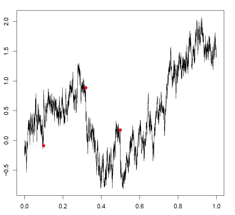
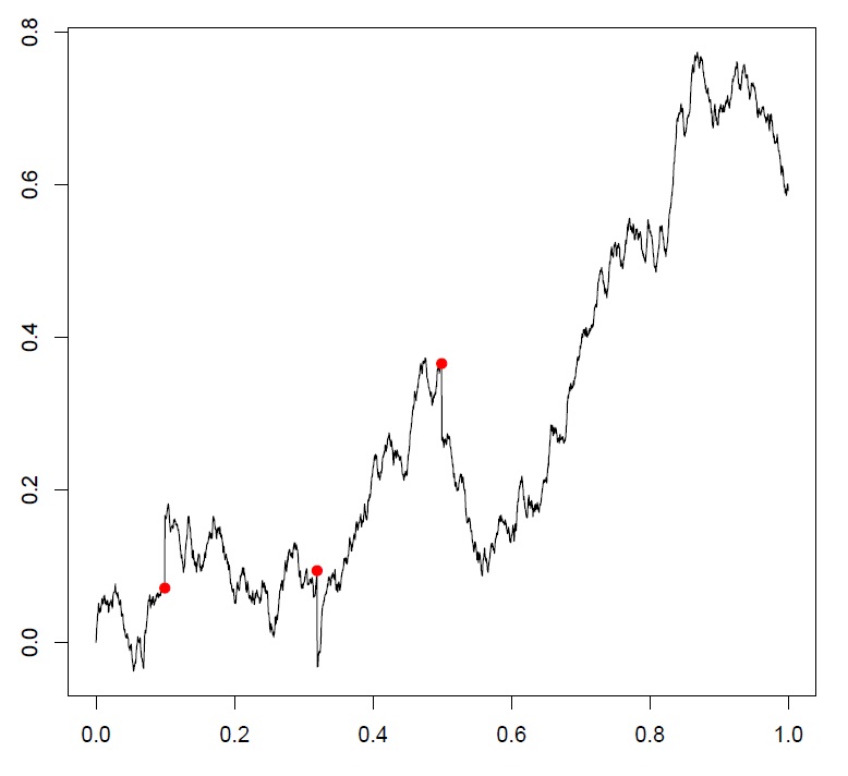
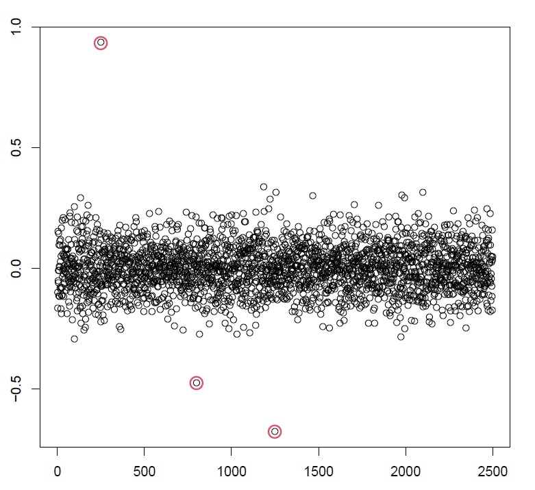
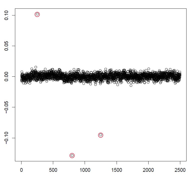
Figure 1: Sample paths (top) and increments (bottom) with $H=0{.3}$ (left) and $H=0{.7}$ (right), and three jumps added which are highlighted by red circles and points.

We formalise our testing problem. When testing for positive jumps, we consider the null hypothesis $H_{0}:w\in\Omega_{0}$, and the alternative hypothesis $H_{1}:w\in\Omega_{+}$, where

$$\Omega_{0}=\left\{w\in\Omega\mid J_{t}(w)=0\text{ for }t\in(0,1]\right\}\quad\text{ and }\quad\Omega_{+}=\left\{w\in\Omega\mid\exists t\in(0,1]:\Delta J_{t}(w)>0\right\}.$$

In the same way, we can define a testing problem for negative jumps, which we omit, since we can treat negative jumps analogously. The testing problem for general jumps is defined with the null hypothesis $H_{0}:w\in\Omega_{0}$ tested against the alternative hypothesis $H_{1}:w\in\Omega_{1}$, where

$$\Omega_{0}=\left\{w\in\Omega\mid J_{t}(w)=0\text{ for }t\in(0,1]\right\}\quad\text{ and }\quad\Omega_{1}=\left\{w\in\Omega\mid\exists t\in(0,1]:\Delta J_{t}(w)\neq 0\right\}.$$

It is not meaningful to consider a jump at time $0$ when we suppose càdlàg jumps. Figure 1 illustrates the intuitive fact that detecting jumps is more difficult when $H$ is small, when the sample paths of $B^{H}$ and $(Y_{t})$ are rougher. Here, we add three jumps to two simulated paths of $B^{H}$, one with $H=0{.3}$ and one with $H=0{.7}$. Comparing increments which include the jumps to other increments of $(Y_{t})$ shows a much larger distance in the smoother example. The values on the $y$-axis also show the sizes of the three jumps which were set much smaller in the smoother case.

2.3 Regularity assumptions

We work under the following regularity assumptions.

Assumption 2.1.

There are three constants $0<V\leq K<\infty$ and $0<\alpha\leq 1$, such that

1. $(\sigma_{s})_{s\in[0,1]}$ is bounded, that is,

   $$0<V\leq\sigma_{s}\leq K,\quad 0\leq s\leq 1,$$

2. $(\sigma_{s})_{s\in[0,1]}$ is Hölder continuous with $\alpha>1-H$, that is,

   $$|\sigma_{t}-\sigma_{s}|\leq K|t-s|^{\alpha},\quad 0\leq s,t\leq 1.$$

Note that the regularity of $(\sigma_{t})$ is already required to ensure that $(Y_{t})$ is well-defined. One can analogously impose these conditions on the squared volatility $(\sigma_{t}^{2})$.

Assumption 2.2.

$(J_{t})_{t\in[0,1]}$ is a pure jump process with càdlàg paths that satisfies for some $p\in(0,1]$ the condition

$$\mathbb{P}\left(\lim_{n\to\infty}\sum_{k=1}^{n}|\Delta_{n,k}^{(1)}J|^{p}<\infty\right)=1.$$

The previous assumption is stronger for smaller $p\in(0,1]$. Jumps of finite variation as a minimal condition will be required to obtain a jump-robust spot volatility estimator for all $H\in(0,1)$. Throughout the manuscript, we use the notation $a_{n}\propto b_{n}$, for sequences $(a_{n})_{n\in\mathds{N}}$ and $(b_{n})_{n\in\mathds{N}}$, if $a_{n}/b_{n}$ tends to some positive constant and the standard notation $\mathcal{O}$ and ${\scriptstyle{\mathcal{O}}}$ for Landau symbols, as well as $\mathcal{O}_{\mathbb{P}}$ and ${\scriptstyle{\mathcal{O}}}_{\mathbb{P}}$ for the stochastic Landau symbols with respect to the probability measure $\mathbb{P}$.

3 Construction of the tests

In this section, we concisely introduce the statistics our tests will be based on. Considering the maximal, standardized, absolute (second-order) increment the question of how to construct a test boils down to the question how to standardize before taking the maximum. The standardization is up to a scaling factor $n^{H}$ basically a spot volatility estimate of $\sigma_{t}$. The standardization with an estimated volatility is crucial for several reasons. First, although the volatility is lower and upper bounded under Assumption 2.1, normalising with the local volatility is important to better detect jumps, since $n^{H}\Delta_{n,k}^{(1)}Y$ is approximately $\mathcal{N}(0,\sigma_{k/n}^{2})$ normally distributed and time-varying volatility levels should not be neglected when comparing the size of the $k$th absolute increment to $n^{-H}\sigma_{k/n}$. Moreover, the standardization yields a pivotal test, that is, the limit distribution under the null hypothesis will not depend on the unknown volatility $(\sigma_{t})$ any more. While in the semimartingale case we could simply consider a non-standardized version $n^{1/2}\max_{k}|\Delta_{n,k}^{(1)}Y|$, if we do not know $H$ the scaling factor $n^{H}$ is unknown and we exploit that the spot volatility estimates contain the same scaling factor $n^{H}$, which hence cancels out.

While some aspects of our tests will be similar to the Gumbel tests within the semimartingale framework by Lee and Mykland, (2008) and Palmes and Woerner, 2016a , the standardization is more crucial and more involved here. In particular, the spot volatility estimation needs to be robust with respect to jumps and we cannot use truncation methods to achieve this. We use power variations with small powers $p\leq 1$, instead of the standard choice $p=2$, and second-order increments instead of increments for the jump-robust estimation of the spot volatility for all possible Hurst exponents $H\in(0,1)$. Denote $C_{p}$ the $p$-th absolute moment of a standard normal distribution, $\mathcal{N}(0,1)$, for some $p\in(0,1]$. For the bandwidth of the local spot volatility estimation, let $(h_{n})_{n\in\mathbb{N}}$ be a sequence of natural numbers with $\lim_{n\to\infty}h_{n}=\infty$ and $\lim_{n\to\infty}n^{-1}h_{n}=0$. The test for positive jumps will be based on the test statistic

$$T_{n}=\max_{k,j}\left(\frac{\Delta_{n,j}^{(2)}X}{\left(h_{n}^{-1}C_{p}^{-1}\sum_{i=(k-1)h_{n}+2}^{kh_{n}}\Big{|}\Delta_{n,i}^{(2)}X\Big{|}^{p}\right)^{\frac{1}{p}}}\right).$$ (1)

To simplify the notation, we use the short notation

$$\max_{k,j}z_{k,j}:=\max_{2\leq j<h_{n}}z_{1,j}\vee\max_{2\leq k\leq m}\left(\max_{(k-1)h_{n}\leq j<kh_{n}}z_{k,j}\right)\vee\max_{mh_{n}\leq j\leq n}z_{m+1,j}\,,$$

where $a\vee b=\max\{a,b\}$, and

$$\max_{k}z_{k}:=\max_{1\leq k\leq m}z_{k},\quad m=\lfloor n/h_{n}\rfloor\,,$$

for some measurable transformations $z_{k,j}$ and $z_{k}$ of increments of our processes. Analogously, testing for jumps will be based on the statistic

$$R_{n}=\max_{k,j}\left(\frac{|\Delta_{n,j}^{(2)}X|}{\left(h_{n}^{-1}C_{p}^{-1}\sum_{i=(k-1)h_{n}+2}^{kh_{n}}\Big{|}\Delta_{n,i}^{(2)}X\Big{|}^{p}\right)^{\frac{1}{p}}}\right).$$ (2)

An optimal bandwidth $h_{n}$ in the normalization factor is given by $h_{n}\propto n^{2\alpha/(2\alpha+1)}$, with the regularity $\alpha$ of $(\sigma_{t})$ from Assumption 2.1. This is obtained from the standard decomposition of the mean squared estimation error in variance and squared bias and balancing both parts. However, the asymptotic results for the tests will not require a rate-optimal volatility estimation and hence we do not need to assume that $\alpha$ is known. We will establish the main results under the condition that $h_{n}\propto n^{\beta}$, with some $\beta$, such that $pH<\beta<1$. This can be ensured by choosing $p$ sufficiently small.

Second-order increments are at first only important in the denominators of (1) and (2) for the jump-robust spot volatility estimation, in particular for large values of $H$. Then, however, we need to take second-order increments in the numerators as well, since $n^{H}\Delta_{n,k}^{(2)}Y$ is approximately $\mathcal{N}(0,\sigma_{k/n}^{2}C_{H})$ distributed, with a constant $C_{H}$ that hinges on $H$. Then, in our ratios, the factors $C_{H}\cdot n^{H}$ cancel out.

The reason that power variations of second-order increments allow to estimate the volatility robust with respect to jumps without any truncation relates to a question which is currently of great interest for the literature on rough volatility models. The question is, if $H$ can be estimated robustly as well, and if ignoring jumps could manipulate estimates of $H$ when applying standard estimators with increments of $(X_{t})$ inserted, while the estimator is actually built for observations of the continuous process $(Y_{t})$. Given the importance of this aspect, we emphasize it in the next section before finishing the construction of our tests.

4 Jump-robust inference on rough processes

For the construction of our test, we require a jump-robust spot volatility estimation. We use an estimator based on power variations of second-order increments and we do not use truncation or bipower variation statistics. The reason why this works relates to jump-robust inference on the Hurst exponent for rough processes based on high-frequency observations. Since we expect that this is of great interest for the current research on rough volatility models, we emphasize here some crucial results on this aspect. In particular, we consider in this section the standard discrete quadratic variation and a standard estimator for the Hurst exponent to analyse the effect of jumps on these statistics.

Proposition 4.1.

If $H\in(0,1/2)$, for a general jump component $(J_{t})$, which is independent of $(Y_{t})$, it holds under Assumption 2.1 that

$$n^{2H-1}\sum_{j=1}^{n}\big{(}\Delta_{n,j}^{(1)}X\big{)}^{2}=\int_{0}^{1}\sigma_{s}^{2}\,\mathrm{d}s+\mathcal{O}_{\mathbb{P}}\big{(}n^{\max((2H-1),-1/2)}\big{)}\,.$$ (3)

In particular, this implies that $n^{2H-1}\sum_{j=1}^{n}\big{(}\Delta_{n,j}^{(1)}X\big{)}^{2}\stackrel{{\scriptstyle\mathbb{P}}}{{\rightarrow}}\int_{0}^{1}\sigma_{s}^{2}\,\mathrm{d}s$, as $n\to\infty$.

This result is based on central limit theorems for power variations of integral fractional processes from Corcuera et al., (2006) and some estimates for the jumps. In fact, the possible robustness with respect to jumps was already mentioned by Corcuera et al., (2006). Contrary to the situation for $H=1/2$, the mean of rescaled squared increments consistently estimates the integrated squared volatility, also in the presence of jumps. This works without truncation. In particular, if $H<1/4$, the central limit theorem for the integrated squared volatility with the standard optimal rate $n^{1/2}$ carries over. The limit theorem is then completely analogous to the continuous case when $(Y_{t})$ is observed and general semimartingale jumps in $(X_{t})$ are asymptotically negligible. If $H>1/2$, the statistic left-hand side in (3) would diverge in the presence of jumps instead. For this reason, we use smaller powers $p$ for our statistical methods in (1) and (2), which should be valid for all $H\in(0,1)$. While smaller $H$ and rougher paths of $(Y_{t})$ make the detection of jumps more difficult, the effect of smaller $H$ on the robustness is positive instead. These effects can be seen as two sides of the same coin. In Figure 1 we see that the influence of increments with jumps becomes smaller compared to other increments when $H$ is smaller. It is thus natural that robustness of non-adjusted statistics – when we ignore jumps – is more likely to hold for smaller $H$. Next, we point out that a standard estimator of the Hurst exponent is robust with respect to jumps without adjustments in the rough case when $H$ is small.

Proposition 4.2.

The estimator of the Hurst exponent,

$$\hat{H}_{n}=\frac{1}{2\log(2)}\log\bigg{(}\frac{\sum_{j=0}^{n-2}\big{(}X_{(j+2)/n}-X_{j/n}\big{)}^{2}}{\sum_{j=0}^{n-1}\big{(}X_{(j+1)/n}-X_{j/n}\big{)}^{2}}\bigg{)}\,,$$ (4)

satisfies under Assumption 2.1 for any $H\in(0,1/2)$, and for any jump semimartingale $(J_{t})$ which is independent of $(Y_{t})$, that

$$\hat{H}_{n}-H=\mathcal{O}_{\mathbb{P}}\big{(}n^{\max((2H-1),-1/2)}\big{)}\,.$$ (5)

In particular, $\hat{H}_{n}$ is a consistent estimator for $H$, $\hat{H}_{n}\stackrel{{\scriptstyle\mathbb{P}}}{{\rightarrow}}H$, as $n\to\infty$. In case that $H\geq 1/2$, and if $(J_{t})$ is an Itô semimartingale with bounded jump sizes, it holds that $\hat{H}_{n}\stackrel{{\scriptstyle\mathbb{P}}}{{\rightarrow}}1/2$, as $n\to\infty$.

We use the notion of Itô semimartingales in the sense of Section 2.1.4 of Jacod and Protter, (2011). These are semimartingales whose characteristics are absolutely continuous with respect to the Lebesgue measure, such that the process admit a representation as Grigelionis processes in the sense of Kallsen, (1998).

Estimator (4) is a rather obvious estimator for $H$ based on power variations, and contained in the class of filtering estimators by Coeurjolly, (2001) setting $k=2$ and $a=(1,-1)$ in his general statistics. With the estimate of $H$, a plug-in approach allows estimating the squared volatility as well. For $H<1/4$, the jump-robust estimator of the Hurst exponent attains the optimal rate of convergence, $n^{-1/2}$, and central limit theorems proved for the continuous case apply. Statistic (4) is indeed a proper estimator, also for unknown $H$ and $(\sigma_{t})$, since $\hat{H}_{n}$ is a function of the observations only. If $(X_{t})$ is used to model the volatility, we conclude that inference on the Hurst exponent under rough volatility is robust with respect to general additive jumps. This is an important insight for the current research on rough volatility. The second result in Proposition 4.2, that $\hat{H}_{n}\stackrel{{\scriptstyle\mathbb{P}}}{{\rightarrow}}1/2$, also in the non-robust case of $H>1/2$, is crucial to conclude that a small estimate of $H$ cannot be produced by jumps and a smoother continuous component. We conjecture that the robustness with respect to jumps can be extended even to a larger range of values of $H$, when using power variations with smaller powers and second-order increments. Since such results require more restrictive assumptions on the jumps and refined proofs, where less existing results can be exploited, we leave this conjecture open for future research. Here we focus on the impact of jumps on the standard methods which are typically used when jumps are ignored. Nevertheless, the robustness is only valid for small $H$ and our simulations will show that jumps might influence the finite-sample estimation. This provides additional motivation to construct jump-detection methods to filter out jumps in case that they are considered to be a nuisance quantity. The methods presented in the upcoming section allow testing for jumps and moreover to locate them and thus also to filter out jumps. Being aware of possible jumps, filtering increments with jumps based on our new methods and applying the standard estimators afterwards hence provides a tractable approach. In particular, for larger $H$, when the non-adjusted estimators for the Hurst exponent and the volatility do not work well, our methods to detect and filter jumps attain a particularly good performance. In this sense, the two reverse effects can be combined to accurately solve the problem of statistical inference across all model specifications.

5 Asymptotic properties of the tests

5.1 Asymptotic distribution under the null hypothesis

In this section, we present our original statistical methods and state the main results of this paper. For the tests, we establish the asymptotic behaviour of the statistics $T_{n}$ from (1) and $R_{n}$ from (2). Our first main result clarifies the asymptotic distributions of $T_{n}$ and $R_{n}$ under the null hypothesis that there are no jumps.

Theorem 1.

Assume that $(\sigma_{t})_{t\in[0,1]}$ satisfies Assumption 2.1. Let $p\in(0,1]$ and set $h_{n}\propto n^{\beta}$, for $0<\beta<1$.

1. Under $H_{0}$, it holds that

   $$\lim_{n\to\infty}\mathbb{P}\left(a_{n}\left(T_{n}-b_{n}\right)\leq x\right)=\exp(-\exp(-x)),\quad\text{ for }x\in\mathbb{R},$$

   with the sequences

   $$a_{n}=\sqrt{2\log(n)},~{}\text{and}~{}~{}b_{n}=\sqrt{2\log(n)}-\frac{\log(\log(n))+\log(4\pi)}{2\sqrt{2\log(n)}}\,.$$

2. Under $H_{0}$, it holds that

   $$\lim_{n\to\infty}\mathbb{P}\left(c_{n}\left(R_{n}-d_{n}\right)\leq x\right)=\exp(-\exp(-x)),\quad\text{ for }x\in\mathbb{R},$$

   with the sequences

   $$c_{n}=\sqrt{2\log(2n)},~{}\text{and}~{}~{}d_{n}=\sqrt{2\log(2n)}-\frac{\log(\log(2n))+\log(4\pi)}{2\sqrt{2\log(2n)}}.$$

The pointwise convergence of the cumulative distribution function shows that convergence in distribution to a standard Gumbel limit distribution is satisfied. The sequences $(a_{n})_{n\in\mathds{N}}$ and $(b_{n})_{n\in\mathds{N}}$ are identical to the ones in the Gumbel convergence of the maximum of i.i.d. standard normal random variables and thus also agree to the ones occurring in Lee and Mykland, (2008). For the sequences $(c_{n})_{n\in\mathds{N}}$ and $(d_{n})_{n\in\mathds{N}}$, factors $n$ are replaced by $2n$, similar as in the Gumbel convergence of the maximum of absolute values of i.i.d. standard normal random variables. Let $q_{\alpha}$ be the $(1-\alpha)$-quantile of the Gumbel distribution:

$$q_{\alpha}=-\log\left(-\log\left(1-\alpha\right)\right).$$

1. Testing for positive jumps, we reject $H_{0}$, if $a_{n}(T_{n}-b_{n})\geq q_{\alpha}$.

2. Testing for jumps, we reject $H_{0}$, if $c_{n}(R_{n}-d_{n})\geq q_{\alpha}$.

For these tests, Theorem 1 readily yields the following asymptotic properties.

Corollary 5.1.

1. The test $\operatorname{(T1)}$ for $H_{0}$ against $H_{1}:w\in\Omega_{+}$ has asymptotic level $\alpha$, as $n\to\infty$.

2. The test $\operatorname{(T2)}$ for $H_{0}$ against $H_{1}:w\in\Omega_{1}$ has asymptotic level $\alpha$, as $n\to\infty$.

5.2 Consistency and rate of convergence under the alternative

For the test, we next clarify the behaviour of the statistics under the alternative hypothesis.

Theorem 2.

Assume that $(\sigma_{t})_{t\in[0,1]}$ satisfies Assumption 2.1 and that Assumption 2.2 is satisfied for some $\tilde{p}\in(0,1]$. Let $0<p\leq\tilde{p}$ and $pH<\beta<1$ and set $h_{n}\propto n^{\beta}$.

1. Under the alternative hypothesis $H_{1}:w\in\Omega_{+}$, it holds true that

   $$\lim_{n\to\infty}\mathbb{P}\left(n^{-\gamma}a_{n}\left(T_{n}-b_{n}\right)\leq L\right)=0,\quad\text{ for all }\quad L\in\mathbb{R}\quad\text{ and }\quad 0<\gamma<H.$$

2. Under the alternative hypothesis $H_{1}:w\in\Omega_{1}$, it holds true that

   $$\lim_{n\to\infty}\mathbb{P}\left(n^{-\gamma}c_{n}\left(R_{n}-d_{n}\right)\leq L\right)=0,\quad\text{ for all }\quad L\in\mathbb{R}\quad\text{ and }\quad 0<\gamma<H.$$

Theorem 2 readily implies the following asymptotic properties of the Gumbel tests.

Corollary 5.2.

1. The test $\operatorname{(T1)}$ for $H_{0}$ against $H_{1}:w\in\Omega_{+}$ is consistent, that is, it has asymptotic power $1$, as $n\to\infty$.

2. The test $\operatorname{(T2)}$ for $H_{0}$ against $H_{1}:w\in\Omega_{1}$ is consistent, that is, it has asymptotic power $1$, as $n\to\infty$.

Moreover, Theorem 2 establishes a rate of convergence for local alternatives. That is, consistency of the tests applies even in case of asymptotically decreasing sequences of (absolute) jump sizes $(|\Delta J_{\tau}|)_{n}$, as long as $\liminf_{n\to\infty}(|\Delta J_{\tau}|)_{n}n^{\gamma}>0$, with arbitrary $\gamma<H$. Since $n^{-H}$ is the size of absolute increments of the continuous component $(Y_{t})$, a faster rate is not possible. As expected, the rate hinges on $H$ and is faster for larger $H$. In Figure 1, we can thus find much smaller jumps in the smoother case on the right than in the rougher example left-hand side.

5.3 Localization of jumps

One crucial advantage of tests for jumps based on maximum statistics as ours, for instance, compared to tests based on fractions of different power variations, is that it readily allows the localization of jumps. That is, the associated $\operatorname{argmax}$ yields a consistent estimator for the time at which a jump occurred. We establish consistency and a fast rate of convergence of order $n$, under the alternative $H_{1}$, when one jump occurred.

Proposition 5.3.

Under $H_{1}$, if there is one jump at time $\tau\in(0,1)$, and $J_{t}=0$, for all $t\neq\tau$, the estimator of the jump time

$$\hat{\tau}_{n}=\frac{1}{n}\operatorname{argmax}_{2\leq j\leq n}\frac{|\Delta_{n,j}^{(2)}X|}{\Big{(}h_{n}^{-1}C_{p}^{-1}\sum_{i=\lfloor jh_{n}^{-1}\rfloor}^{\lfloor jh_{n}^{-1}\rfloor+h_{n}}|\Delta_{n,j}^{(2)}X|^{p}\Big{)}^{1/p}}\,,$$

satisfies under the conditions of Theorem 2 that

$$\big{(}\hat{\tau}_{n}-\tau\big{)}=\mathcal{O}_{\mathbb{P}}\big{(}n^{-1}\big{)}\,.$$

Clearly, based on discrete observation times with distance $n^{-1}$, it is impossible to locate jumps more accurately than in a $n^{-1}$-neighbourhood of $\tau$. As the proof of the proposition shows, this works even for decreasing sequences of absolute jump sizes $(|\Delta J_{\tau}|)_{n}$, as long as $\liminf_{n\to\infty}(|\Delta J_{\tau}|)_{n}n^{\gamma}>0$, for some $\gamma<H$. Thus, we can estimate jump times with the best possible rate of convergence. Confidence for $\operatorname{argmax}$-estimators is, however, a very involved problem which is beyond the scope of this manuscript.
A sequential application of the test based on the maximum and the $\operatorname{argmax}$-estimator, where we discard in each step the previous maximal absolute (second-order) increment, yields a sequential top-down algorithm that consistently estimates the correct number and times of jumps under $H_{1}$, if we assume some finite number of jumps. It is possible to combine our theory with standard concepts from multiple testing to control the overall error probability of a sequential test. Furthermore, the maximal absolute increments and their signs yield estimates of jump sizes as well.

6 Simulations

In this section, we investigate the finite-sample properties of our test and the estimation of the Hurst exponent in the presence of jumps in a Monte Carlo simulation study. We implement the model with the volatility function

$$\sigma_{t}=1-0{.}2\cdot\sin\left(\frac{3}{4}\pi t\right),\quad t\in[0,1],$$

which is a Lipschitz continuous function, such that we have $\alpha=1$ in Assumption 2.1. Therefore, we choose the optimal bandwidth $h_{n}=\lfloor n^{2/3}\rfloor$, with $\beta=2/3$, for spot volatility estimation. For the simulation of paths of the fractional Brownian motion, we are using the Cholesky method as described in Section 3.4 of Coeurjolly, (2000). We will only illustrate the finite-sample properties of the test $\operatorname{(T1)}$ based on $T_{n}$ from (1). The results for the test $\operatorname{(T2)}$ based on $R_{n}$ from (2) are completely analogous and hence omitted.

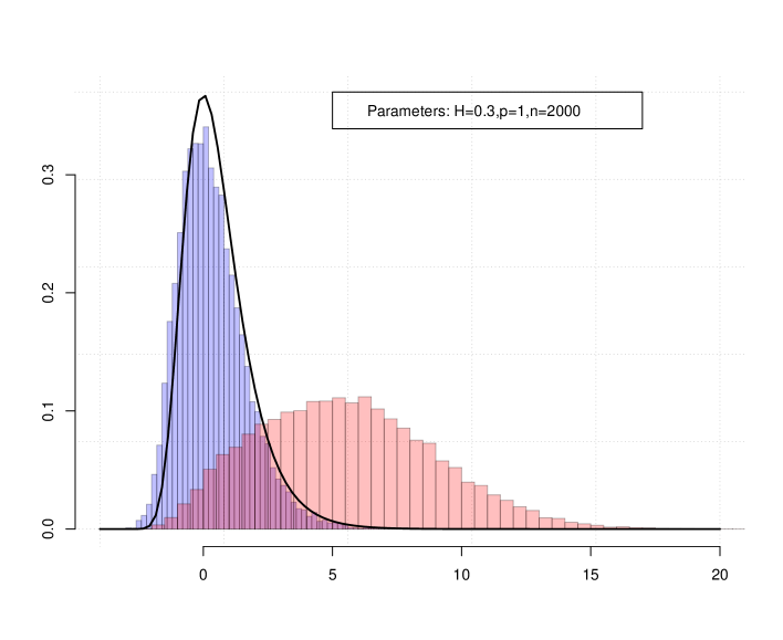
Figure 2: Empirical distributions of test statistic under the null hypothesis, compared to the standard Gumbel limit distribution drawn with the black line, and under the alternative hypothesis with fix jump size $\Delta J_{\tau}=0{.}8$.

Figure 2 visualizes the empirical distribution of the test statistic for the test $\operatorname{(T1)}$ in the left histogram under the null hypothesis. The histograms are standardised to densities and we draw a comparison to the density of the theoretical, standard Gumbel limit distribution which is drawn with a solid black line. Both histograms in Figure 2 are based on 2000 Monte Carlo runs of our model with $H=0{.}3$, and for sample size $n=2000$. The empirical quantiles match reasonably well with those of the Gumbel density. Although the finite-sample fit is not perfect, in particular the large quantiles closely track their theoretical asymptotic counterparts. We conclude that we can use the test as constructed without finite-sample adjustments as, for instance, a bootstrapped version. The right histogram in Figure 2 shows the empirical distribution of the test statistic under the alternative hypothesis with a fixed jump size of $0{.}8$, at a generated jump time $\tau$, which is uniformly distributed on $\{1/n,\ldots,(n-1)/n\}$. In this setting, the empirical distributions under the null and alternative hypotheses separate, but the power of the test does not attain a value close to 1. We can see this in Figure 2, since the two histograms overlap.

Figure 3: Empirical power against level $\gamma$ of jump sizes $\sqrt{2\log(n)}n^{-\gamma}$.

We consider one jump at a uniformly distributed jump time to demonstrate the power of our test in a finite sample. The empirical power of the test for positive jumps with level 5% is illustrated for jump sizes $\sqrt{2\log(n)}n^{-\gamma}$, with different values of $0<\gamma<H$, in Figure 3 with a sample size $n=2000$. One of our main theoretical results shows that for jump sizes with $\gamma<H$ our test $\operatorname{(T1)}$ should start to work with increasing power as $\gamma$ decreases. Figure 3 confirms the expected behaviour, for $H=0{.}3$ right-hand side and $H=0{.}7$ left-hand side, and the power increases rapidly with decreasing values of $\gamma$. We use statistic (1) with $p=1$ for $H=0{.}3$, and with $p=0{.}9$ for $H=0{.}7$, such that the condition $pH<\beta=2/3$ from Theorem 2 is satisfied in both cases. Using smaller values of $p$ yields similar empirical results. Comparing the associated jump sizes for certain powers in the two plots of Figure 3 underlines the fact that larger $H$, resulting in smoother paths of $(Y_{t})$, allows to detect much smaller jumps. The setting of Figure 2 corresponds to $\gamma\approx 0{.}21$, and the plot right-hand side in Figure 3 shows that the power is slightly below 80% in this case.

Tables 2 and 2 contain the empirical powers for different jump sizes and different sample sizes. In each scenario, the jump size is kept fix and the time of the jump is uniformly distributed. In each column, for fixed jump sizes, the empirical power increases from top down when the sample size is increasing. In each row, for fixed sample sizes, the empirical power increases from left to right when the jump size is increasing.

	$0.013$	$0.015$	$0.017$	$0.019$	$0.020$	$0.022$	$0.024$	$0.026$	$0.028$	$0.029$
$500$	0.046	0.046	0.046	0.046	0.047	0.049	0.051	0.053	0.058	0.063
$1000$	0.049	0.052	0.054	0.059	0.065	0.091	0.101	0.127	0.163	0.200
$1500$	0.049	0.060	0.081	0.107	0.143	0.197	0.255	0.341	0.434	0.519
$2000$	0.073	0.107	0.148	0.210	0.287	0.394	0.504	0.616	0.730	0.825
$2500$	0.102	0.166	0.251	0.362	0.493	0.625	0.751	0.846	0.921	0.961

Table 1: Empirical power for Hurst exponent $H=0{.}7$ based on $2000$ Monte Carlo simulations. $\Delta J_{\tau}$ denotes the jump size, starting around $2500^{-0.67}\sqrt{2\log(2500)}\approx 0.013$. We use (1) with $p=0{.}9$.

	$0.360$	$0.415$	$0.470$	$0.525$	$0.580$	$0.635$	$0.690$	$0.745$	$0.800$	$0.855$
$500$	0.047	0.053	0.059	0.080	0.098	0.118	0.152	0.188	0.237	0.289
$1000$	0.057	0.069	0.083	0.109	0.156	0.199	0.279	0.346	0.449	0.551
$1500$	0.059	0.075	0.102	0.147	0.205	0.272	0.373	0.503	0.613	0.708
$2000$	0.070	0.096	0.140	0.209	0.296	0.400	0.515	0.628	0.740	0.826
$2500$	0.072	0.105	0.161	0.244	0.353	0.477	0.617	0.733	0.828	0.910

Table 2: Empirical power for Hurst exponent $H=0{.}3$ based on $2000$ Monte Carlo simulations. $\Delta J_{\tau}$ denotes the jump size, starting around $2500^{-0.25}\sqrt{2\log(2500)}\approx 0{.}36$. We use (1) with $p=0{.}9$.

To evaluate our test, we further compare the rejection rates under the null hypothesis for the test $\operatorname{(T1)}$ used with the quantile $q_{0.95}=-\log(-\log(0.95))$ of the theoretical Gumbel limit distribution. Table 3 contains the empirical levels, that is, the size of the test, for different Hurst exponents and different sample sizes. These values indicate that our test attains the corresponding level in a finite sample. In fact, the empirical rejection rates are even slightly smaller than the 5% level.

	$500$	$1000$	$1500$	$2000$	$2500$
$0.3$	0.0306	0.0418	0.0380	0.0392	0.0372
$0.7$	0.0430	0.0428	0.0408	0.0386	0.0348

Table 3: Empirical size of the test calculated from $5000$ Monte Carlo simulations. For $H=0{.3}$ we use $p=1$ and and for $H=0{.}7$ we use $p=0{.}9$ in (1).

Figure 4: Empirical robustness in estimating the Hurst exponent.

We study the finite-sample distribution of the estimator (4) to analyse its robustness with respect to jumps. Figure 4 shows boxplots of the estimates for three different values of the Hurst exponent, $H=0{.}2$, $H=0{.}4$, and $H=0{.}6$. For each value of $H$, we add one jump to the simulated paths of $(X_{t})$ at a uniformly distributed jump time and we consider an increasing sequence of jump sizes starting with a very small one of size $\Delta J_{\tau}=0{.}1$, up to a huge jump of size $\Delta J_{\tau}=2{.}5$. Each boxplot is based on 2000 Monte Carlo runs and the sample size is in all scenarios $n=2000$. We directly apply estimator (4), without filtering jumps, to demonstrate the effects of ignoring jumps on the estimation of the Hurst exponent. This seems to be important to us in view of the existing literature and empirical evidence for rough volatility.

For $H=0{.}2$, by the theoretical result of Proposition 4.2 the estimator is consistent, also in presence of jumps, and even satisfies the central limit theorem at optimal rate $\sqrt{n}$. The robustness is confirmed in the finite-sample simulation left in Figure 4, at least for moderate jump sizes. Huge jumps can, however, result in a positive finite-sample bias. One implication of this finding is that filtering jumps based on our methods is beneficial for estimating the Hurst exponent and can increase the finite-sample precision, also for small values of the true Hurst exponent. Another important insight is that a finite-sample bias due to jumps is positive and thus jumps cannot manipulate estimates of $H$ in the way that smaller estimates are obtained. A positive bias is expected from the theory, since the jumps inserted in the estimator (4) yield the value 1/2. Therefore, the empirical means should lie between 1/2 and the unbiased estimates based on the observations of the continuous component $(Y_{t})$. This is more good news for the literature pointing at empirical evidence for rough volatility. Ignoring jumps cannot result in a negative bias of their estimated Hurst exponents, at least when using the estimator (4) or similar ones.

For $H=0{.}4$, by Proposition 4.2 consistency of the estimator does still hold. The convergence rate is however slower in these scenarios and the central limit theorem which would hold for observations of $(Y_{t})$ without jumps does not remain valid in presence of jumps. The few outliers we see for $H=0{.}4$ and $H=0{.}6$ in Figure 4 are due to jumps with a jump time that falls in the last observed increment. In this case, the jumps inserted in the estimator (4) yield the value 0 instead of 1/2, what explains the smaller estimates in these cases. Compared to the smaller Hurst exponent, the positive finite-sample bias with increasing jump size is much more pronounced here. Filtering jumps before the estimation of $H$ is thus even more important. The localization based on our methods from Section 5.3 yields the correct jump times, referring to the correct discrete index of the second-order increments containing the jumps, in basically all cases in that the test rejects correctly. Since the power of our test is high for the larger jump sizes, pre-filtering jumps with our methods would correct the finite-sample bias in the estimates of Figure 4.

Finally, on the right in Figure 4 we apply estimator (4) to paths of $(X_{t})$ with jumps and $H=0{.}6$. Proposition 4.2 shows that the estimator is here inconsistent and converges to 1/2 in probability instead of $0{.}6$. We see this for larger jumps and that the variance of the estimation becomes small when the jumps dominate the continuous component in the finite-sample, empirical distribution. Only for very small jumps, the estimation is still robust with respect to jumps for this fixed sample size.

In conclusion, Figure 4 underlines our finding that ignoring jumps could not manipulate the empirical evidence for rough volatility obtained so far. At the same time, it motivates that filtering jumps is nevertheless important, also when estimation of $H$ is the main target. Our proposed test with the localization procedure can be used to filter out the jumps. After discarding the largest absolute second-order increments which our test ascribes to jumps only the remaining second-order increments should be used for estimators as (4).

7 Conclusion

We have solved the problem of testing for jumps based on high-frequency observations of a process with integral fractional part and present a Gumbel test with the desired asymptotic properties. We pointed at good news for the rough volatility literature, that jumps do not manipulate their empirical finding that volatility is rough. For future research, it will be of interest to strengthen and generalize our results on the robustness of inference on $H$ and $(\sigma_{t})$ with respect to jumps. We provide a localization result about the optimal estimation of jump times. This is new also for the semimartingale case, as such a result was not contained in the existing literature. It can be used to filter out jumps when the goal is inference on $H$ and $(\sigma_{t}^{2})$. Since the power of our approach increases with $H$, it works in particular well in the case when non-adjusted statistics for the continuous model without jumps become inconsistent. However, asymptotic results for using the suggested top-down algorithm are readily feasible from our theory only when restricting to jumps of finite activity. Therefore, a more general solution to the problem of estimation of $H$ and $(\sigma_{t})$ under jumps remains an open question. For this purpose, it might be worth exploring approaches as multipower variations or a global jump filter, considered in Barndorff-Nielsen et al., (2011), Barndorff-Nielsen et al., (2006) and Inatsugu and Yoshida, (2021) for Brownian semistationary processes and semimartingales, respectively. To model a volatility which has to be pre-estimated from observed prices, it would be of interest to further extend the methods to an observation model with additional noise. The Gumbel test for jump diffusion models has been extended to a noisy observation model in Lee and Mykland, (2012).

8 Proofs

8.1 Groundwork from extreme value theory

We require a result that the well-known Gumbel convergence for the maximum of i.i.d.  standard normally distributed random variables generalizes to stationary sequences of weakly dependent normally distributed random variables.

Lemma 8.1.

Let $(Y_{n})_{n\in\mathbb{N}}$ be a standardised stationary sequence of normally distributed random variables, such that $\mathbb{E}[Y_{n}]=0$ and $\mathbb{V}\textnormal{a\hskip 0.56917ptr}(Y_{n})=1$, with covariances $(\gamma(n))_{n\in\mathbb{N}}$ satisfying the condition $\lim_{n\to\infty}\log(n)\gamma(n)=0$. Then it holds that

$$\lim_{n\to\infty}\mathbb{P}\left(a_{n}\left(\max_{1\leq k\leq n}Y_{k}-b_{n}\right)\leq x\right)=\exp\left(-\exp(-x)\right),\quad x\in\mathbb{R},$$

where $a_{n}$ and $b_{n}$ are given by

$$a_{n}=\sqrt{2\log(n)},\quad b_{n}=a_{n}-\frac{\log(\log(n))+\log(4\pi)}{2a_{n}}.$$

Furthermore if we define $c_{n}$ and $d_{n}$ by

$$c_{n}=\sqrt{2\log(2n)},\quad d_{n}=c_{n}-\frac{\log(\log(2n))+\log(4\pi)}{2c_{n}},$$

we obtain that

$$\lim_{n\to\infty}\mathbb{P}\left(c_{n}\left(\max_{1\leq k\leq n}|Y_{k}|-d_{n}\right)\leq x\right)=\exp\left(-\exp(-x)\right),\quad x\in\mathbb{R}.$$

The first part is Theorem 3.1 from Berman, (1964). The second part is readily implied by the symmetry of the standard normal distribution.

Lemma 8.2 (Rescaled Minima).

Let $(Y_{n})_{n\geq 1}$ be a stationary sequence of normally distributed random variables with $\mathbb{E}[Y_{n}]=0$, and with

$$\lim_{n\to\infty}\mathbb{P}\left(a_{n}\left(\max_{1\leq k\leq n}Y_{k}-b_{n}\right)\leq x\right)=\exp(-\exp(-x)),\quad x\in\mathbb{R},$$

where $a_{n}$ and $b_{n}$ are given by

$$a_{n}=\sqrt{2\log(n)},\quad b_{n}=a_{n}-\frac{\log(\log(n))+\log(4\pi)}{2a_{n}}.$$

Then it holds as well that

$$\lim_{n\to\infty}\mathbb{P}\left(a_{n}\left(\min_{1\leq k\leq n}Y_{k}+b_{n}\right)\leq x\right)=1-\exp(-\exp(x)),\quad x\in\mathbb{R}.$$

Proof.

By the symmetry of the normal distribution, the following equalities in distribution hold true:

$$\min_{1\leq k\leq n}Y_{k}\stackrel{{\scriptstyle d}}{{=}}\min_{1\leq k\leq n}-Y_{k}\stackrel{{\scriptstyle d}}{{=}}-\max_{1\leq k\leq n}Y_{k}.$$

Therefore, we conclude that

$$\lim_{n\to\infty}\mathbb{P}\left(a_{n}\left(\min_{1\leq k\leq n}Y_{k}+b_{n}\right)\leq x\right) = 1-\lim_{n\to\infty}\mathbb{P}\left(a_{n}\left(\max_{1\leq k\leq n}Y_{k}-b_{n}\right)\leq-x\right)$$

$$= 1-\exp(-\exp(x)).$$

∎

8.2 Asymptotic behaviour of the normalization and spot volatility estimator

Throughout this section, $K_{1}$ and $K_{2}$ denote positive constants, which can change from line to line. $C_{p}$ denotes the $p$-th absolute moment of a standard Gaussian distribution, $p\in(0,1]$. Set $C_{H}=(4-2^{2H})$ for $H\in(0,1)$. This constant occurs in the variance of second-order increments of fractional Brownian motion, $\mathbb{E}[(\Delta_{n,2}^{(2)}B^{H})^{2}]=C_{H}n^{-2H}$. For $(h_{n})_{n\in\mathbb{N}}$ a sequence of natural numbers with $\lim_{n\to\infty}h_{n}=\infty$, and $\lim_{n\to\infty}n^{-1}h_{n}=0$, we define for $p\in(0,1]$,

$$\widehat{\sigma_{(kh_{n})/n}^{p}}=n^{pH}h_{n}^{-1}C_{p}^{-1}\sum_{j=(k-1)h_{n}+2}^{kh_{n}}\Big{|}\Delta_{n,j}^{(2)}X\Big{|}^{p},\quad k=1,\ldots,\lfloor n/h_{n}\rfloor.$$ (6)

We first consider the asymptotic behaviour of this normalization factor under the null hypothesis of no jumps. The statistic $\widehat{\sigma_{(kh_{n})/n}^{p}}$ is in fact a consistent estimator for $C_{H}^{\frac{p}{2}}\sigma_{(kh_{n})/n}^{p}$. We determine next bounds for the bias and the variance of this estimation.

Lemma 8.3 (Bias).

Assume that $(\sigma_{s})_{s\in[0,1]}$ satisfies Assumption 2.1. If $J_{t}=0$, for every $t\in[0,1]$, it holds true that

$$\left(\mathbb{E}\left[\widehat{\sigma_{(kh_{n})/n}^{p}}\right]-C_{H}^{\frac{p}{2}}\sigma_{(kh_{n})/n}^{p}\right)^{2}=\mathcal{O}\left(n^{-2p\alpha}\right)+\mathcal{O}\Big{(}\Big{(}\frac{h_{n}}{n}\Big{)}^{2\alpha}\Big{)},\quad k=1,\ldots,\lfloor n/h_{n}\rfloor.$$

Proof.

Define

$$A_{n}=\bigg{(}n^{pH}h_{n}^{-1}C_{p}^{-1}\sum_{j=(k-1)h_{n}+2}^{kh_{n}}\Big{(}\Big{|}\Delta_{n,j}^{(2)}X\Big{|}^{p}-\sigma_{(j-1)/n}^{p}\Big{|}\Delta_{n,j}^{(2)}B^{H}\Big{|}^{p}\Big{)}\bigg{)}$$

and

$$B_{n}=\bigg{(}n^{pH}h_{n}^{-1}C_{p}^{-1}\sum_{j=(k-1)h_{n}+2}^{kh_{n}}\sigma_{(j-1)/n}^{p}\mathbb{E}\left[\Big{|}\Delta_{n,j}^{(2)}B^{H}\Big{|}^{p}\right]-C_{H}^{\frac{p}{2}}\sigma_{(kh_{n})/n}^{p}\bigg{)}.$$

Using standard estimates, we see that it is enough to show that the following two inequalities hold:

$$\mathbb{E}[A_{n}^{2}]\leq K_{1}n^{-2p\alpha}\quad\text{ and }\quad B_{n}^{2}\leq K_{2}\left(\frac{h_{n}}{n}\right)^{2\alpha}.$$

Writing second-order increments as the differences of first-order increments, a standard inequality yields that

$$A_{n} \leq n^{pH}h_{n}^{-1}C_{p}^{-1}\sum_{j=(k-1)h_{n}+2}^{kh_{n}}\Big{|}\Delta_{n,j}^{(1)}X-\sigma_{(j-1)/n}\Delta_{n,j}^{(1)}B^{H}\Big{|}^{p}$$

$$+ n^{pH}h_{n}^{-1}C_{p}^{-1}\sum_{j=(k-1)h_{n}+2}^{kh_{n}}\Big{|}\Delta_{n,j-1}^{(1)}X-\sigma_{(j-1)/n}\Delta_{n,j-1}^{(1)}B^{H}\Big{|}^{p}\,.$$

Now, the Love-Young inequality, see Theorem 1.16 in Kubilius et al., (2017) for an exact formulation, implies that

$$\Big{|}\Delta_{n,j}^{(1)}X-\sigma_{(j-1)/n}\Delta_{n,j}^{(1)}B^{H}\Big{|}^{p}\leq C(p,\alpha,H)n^{-p(\alpha+H)}$$

uniformly for all $j$, and analogously with the shifted increments that

$$\Big{|}\Delta_{n,j-1}^{(1)}X-\sigma_{(j-1)/n}\Delta_{n,j-1}^{(1)}B^{H}\Big{|}^{p}\leq C(p,\alpha,H)n^{-p(\alpha+H)},$$

where $C(p,\alpha,H)$ is a positive constant, which comes from the Hölder continuity of the fractional Brownian motion and $(\sigma_{s})_{s\in[0,1]}$. Note that the constant coming from the Hölder continuity of $(\sigma_{s})_{s\in[0,1]}$ is bounded by Assumption 2.1 and that, by Theorem 1 of Azmoodeh et al., (2014), the constant coming from the Hölder continuity of the fractional Brownian motion has moments of all order. Thus, we conclude that

$$\mathbb{E}[A_{n}^{2}] \leq 2\mathbb{E}\left[\left(n^{pH}h_{n}^{-1}C_{p}^{-1}\sum_{j=(k-1)h_{n}+2}^{kh_{n}}\Big{|}\Delta_{n,j}^{(1)}X-\sigma_{(j-1)/n}\Delta_{n,j}^{(1)}B^{H}\Big{|}^{p}\right)^{2}\right]$$

$$+ 2\mathbb{E}\left[\left(n^{pH}h_{n}^{-1}C_{p}^{-1}\sum_{j=(k-1)h_{n}+2}^{kh_{n}}\Big{|}\Delta_{n,j-1}^{(1)}X-\sigma_{(j-1)/n}\Delta_{n,j-1}^{(1)}B^{H}\Big{|}^{p}\right)^{2}\right]\leq K_{1}n^{-2p\alpha}.$$

Applying the Cauchy-Schwarz inequality and the Hölder continuity of $(\sigma_{s}^{p})_{s\in[0,1]}$, yields that

$$B_{n}^{2} = \bigg{(}C_{H}^{\frac{p}{2}}h_{n}^{-1}\sum_{j=(k-1)h_{n}+2}^{kh_{n}}\left(\sigma_{(j-1)/n}^{p}-\sigma_{(kh_{n})/n}^{p}\right)\bigg{)}^{2}$$

$$\leq C_{H}^{p}h_{n}^{-1}\sum_{j=(k-1)h_{n}+1}^{kh_{n}}\left(\sigma_{(j-1)/n}^{p}-\sigma_{(kh_{n})/n}^{p}\right)^{2}$$

$$\leq K_{2}h_{n}^{-1}\sum_{j=(k-1)h_{n}+1}^{kh_{n}}\left(\frac{kh_{n}}{n}-\frac{j-1}{n}\right)^{2\alpha}$$

$$\leq K_{2}\left(\frac{h_{n}}{n}\right)^{2\alpha}.$$

∎

Lemma 8.4 (Variance).

Assume that $(\sigma_{s})_{s\in[0,1]}$ satisfies Assumption 2.1. If $J_{t}=0$, for every $t\in[0,1]$, it holds true that

$$\mathbb{V}\text{ar}\left(\widehat{\sigma_{(kh_{n})/n}^{p}}\right)=\mathcal{O}(n^{-2p\alpha})+\mathcal{O}(h_{n}^{-1}),\quad k=1,\ldots,\lfloor n/h_{n}\rfloor.$$

Proof.

Consider $A_{n}$ from the previous proof and define

$$C_{n}=\bigg{(}n^{pH}h_{n}^{-1}C_{p}^{-1}\sum_{j=(k-1)h_{n}+2}^{kh_{n}}\sigma_{(j-1)/n}^{p}\left(\Big{|}\Delta_{n,j}^{(2)}B^{H}\Big{|}^{p}-\mathbb{E}\left[\Big{|}\Delta_{n,j}^{(2)}B^{H}\Big{|}^{p}\right]\right)\bigg{)}.$$

Using standard estimates, we see that it is enough to show that the following two inequalities hold:

$$\mathbb{E}[A_{n}^{2}]\leq K_{1}n^{-2p\alpha}\quad\text{ and }\quad\mathbb{E}[C_{n}^{2}]\leq K_{2}h_{n}^{-1}.$$

The first one is established in the previous proof. We are left to prove the second one. In the sequel, we will exploit the self-similarity of fractional Brownian motion for a convenient notation and therefore consider our fractional Brownian motion $B^{H}$ defined for all times $t\in[0,\infty)$. In line with our notation for second-order increments from Section 2.1, we write

$$\Delta_{1,j}^{(2)}B^{H}=B^{H}_{j}-2B^{H}_{j-1}+B^{H}_{j-2}~{}\mbox{, for}~{}j\in\mathds{N}.$$ (7)

Next, define

$$\rho(k)=\mathbb{C}\text{ov}\left(\Delta_{1,j+k}^{(2)}B^{H},\Delta_{1,j}^{(2)}B^{H}\right),~{}\rho(-k)=\rho(k),\quad\text{ for }k\in\mathds{N},$$

and then use a minor modification of Proposition 5.2.4 from Pipiras and Taqqu, (2017), to obtain that

$$\mathbb{E}[C_{n}^{2}] = C_{p}^{-2}h_{n}^{-2}\sum_{j=2}^{h_{n}}\sum_{i=2}^{h_{n}}\sigma_{(j-1)/n}^{p}\sigma_{(i-1)/n}^{p}\mathbb{C}\text{ov}\left(\Big{|}\Delta_{1,j}^{(2)}B^{H}\Big{|}^{p},\Big{|}\Delta_{1,i}^{(2)}B^{H}\Big{|}^{p}\right)$$

$$\leq K_{2}C_{p}^{-2}h_{n}^{-2}\sum_{j=2}^{h_{n}}\sum_{i=2}^{h_{n}}\sigma_{(j-1)/n}^{p}\sigma_{(i-1)/n}^{p}(\rho(j-i))^{2}$$

$$\leq K_{2}C_{p}^{-2}K^{2p}h_{n}^{-2}\sum_{k=-(h_{n}-2)}^{h_{n}-2}(h_{n}-|k|)(\rho(k))^{2}$$

$$\leq K_{2}C_{p}^{-2}K^{2p}h_{n}^{-1}\sum_{k\in\mathbb{Z}}(\rho(k))^{2}\,.$$

Since $(\rho(n))^{2}\propto n^{4H-8}$, see, for instance, Lemma 1 in Coeurjolly, (2001), the last sum is finite and we get the desired result. ∎

The bias-variance decomposition readily allows finding an optimal choice of $h_{n}$, which minimises the mean squared error.

Corollary 8.5.

Assume that $(\sigma_{s})_{s\in[0,1]}$ satisfies Assumption 2.1. If we further assume that $h_{n}$ satisfies the condition $h_{n}\propto n^{2\alpha/(2\alpha+1)}$ and that $J_{t}=0$, for every $t\in[0,1]$, it holds true that

$$\mathbb{V}\text{ar}\left(\widehat{\sigma_{(kh_{n})/n}^{p}}\right)+\left(\mathbb{E}\left[\widehat{\sigma_{(kh_{n})/n}^{p}}\right]-C_{H}^{\frac{p}{2}}\sigma_{(kh_{n})/n}^{p}\right)^{2}=\mathcal{O}\left(n^{-\left(\frac{2\alpha}{2\alpha+1}\wedge p\alpha\right)}\right),\quad k=1,\ldots,\lfloor n/h_{n}\rfloor.$$

To prepare the proof of consistency of our test under the alternative hypothesis, we have to show that the normalization with the estimated spot volatility is sufficiently robust with respect to the additive jump component $(J_{t})$. This will be formalised in the next lemma.

Lemma 8.6.

Suppose Assumption 2.1 and that Assumption 2.2 is satisfied for some $\tilde{p}\in(0,1]$. Let $0<p\leq\tilde{p}$ and $pH<\beta<1$. Then for $h_{n}\propto n^{\beta}$, it holds that

$$\max_{k}\bigg{|}n^{pH}\sum_{j=(k-1)h_{n}+2}^{kh_{n}}\frac{\left(\Big{|}\Delta_{n,j}^{(2)}X\Big{|}^{p}-\Big{|}\Delta_{n,j}^{(2)}Y\Big{|}^{p}\right)}{h_{n}C_{p}}\bigg{|}={\scriptstyle{\mathcal{O}}}_{\mathbb{P}}(n^{-\gamma})\quad\text{for}\quad 0<\gamma<\beta-pH.$$

Proof.

Under the stated conditions, we have that $\lim_{n\to\infty}n^{pH}h_{n}^{-1}=0$. Therefore, it is enough to show that

$$\bigg{|}\Big{|}\Delta_{n,j}^{(2)}X\Big{|}^{p}-\Big{|}\Delta_{n,j}^{(2)}Y\Big{|}^{p}\bigg{|}\leq\Big{|}\Delta_{n,j}^{(1)}J\Big{|}^{p}+\Big{|}\Delta_{n,j-1}^{(1)}J\Big{|}^{p}.$$

Define $A_{j}=\left\{\Big{|}\Delta_{n,j}^{(2)}X\Big{|}^{p}>\Big{|}\Delta_{n,j}^{(2)}Y\Big{|}^{p}\right\}$ and note that

$$\Big{|}\Big{|}\Delta_{n,j}^{(2)}X\Big{|}^{p}-\Big{|}\Delta_{n,j}^{(2)}Y\Big{|}^{p}\Big{|}\cdot(\mathbbm{1}_{A_{j}}+\mathbbm{1}_{A_{j}^{c}})\leq\Big{|}\Delta_{n,j}^{(2)}J\Big{|}^{p},$$

where the last inequality follows from the fact that $f(x)=|x|^{p}$ is subadditive with the two inequalities

$$\Big{|}\Delta_{n,j}^{(2)}X\Big{|}^{p}\leq\Big{|}\Delta_{n,j}^{(2)}Y\Big{|}^{p}+\Big{|}\Delta_{n,j}^{(2)}J\Big{|}^{p}\quad\text{ and }\quad\Big{|}\Delta_{n,j}^{(2)}Y\Big{|}^{p}-\Big{|}\Delta_{n,j}^{(2)}J\Big{|}^{p}\leq\Big{|}\Delta_{n,j}^{(2)}X\Big{|}^{p}.$$

Applying the subadditivity to $|\Delta_{n,j}^{(2)}J|^{p}$ yields the result. ∎

For the proof of the Gumbel convergence, we will use uniform consistency of the spot volatility estimation, or that the normalising factors converge uniformly in probability, respectively. The next lemma will clarify this statement.

Lemma 8.7.

Assume that $(\sigma_{t})_{t\in[0,1]}$ satisfies Assumption 2.1.

1. Let $p\in(0,1]$ and set $h_{n}\propto n^{\beta}$, for $0<\beta<1$. If $J_{t}=0$, for all $t\in[0,1]$, it holds for $0<\beta_{1}<\beta/2$ and $0<\beta_{2}<p\alpha$, that

   $$\max_{k}\Big{|}\widehat{\sigma_{(kh_{n})/n}^{p}}-C_{H}^{\frac{p}{2}}\sigma_{(kh_{n})/n}^{p}\Big{|}={\scriptstyle{\mathcal{O}}}_{\mathbb{P}}(n^{-(\beta_{1}\wedge\beta_{2})}).$$

2. Assume that Assumption 2.2 is satisfied for some $\tilde{p}\in(0,1]$. Let $0<p\leq\tilde{p}$ and $pH<\beta<1$ and set $h_{n}\propto n^{\beta}$. Then for $0<\beta_{1}<\beta/2$, $0<\beta_{2}<p\alpha$, and $0<\beta_{3}<\beta-pH$, it holds that

   $$\max_{k}\Big{|}\widehat{\sigma_{(kh_{n})/n}^{p}}-C_{H}^{\frac{p}{2}}\sigma_{(kh_{n})/n}^{p}\Big{|}={\scriptstyle{\mathcal{O}}}_{\mathbb{P}}(n^{-(\beta_{1}\wedge\beta_{2}\wedge\beta_{3})}).$$

Proof.

We will prove the first part of the lemma. The second part can be shown analogously. Using standard inequalities for maxima and the reverse triangle inequality, we get the following estimate

$$\max_{k}\Big{|}n^{pH}h_{n}^{-1}C_{p}^{-1}\sum_{j=(k-1)h_{n}+2}^{kh_{n}}\Big{|}\Delta_{n,j}^{(2)}X\Big{|}^{p}-C_{H}^{\frac{p}{2}}\sigma_{(kh_{n})/n}^{p}\Big{|}$$

$$\leq \max_{k}n^{pH}h_{n}^{-1}C_{p}^{-1}\sum_{j=(k-1)h_{n}+2}^{kh_{n}}\Big{|}\Delta_{n,j}^{(1)}X-\sigma_{(j-1)/n}\left(\Delta_{n,j}^{(1)}B^{H}\right)\Big{|}^{p}$$

$$+ \max_{k}n^{pH}h_{n}^{-1}C_{p}^{-1}\sum_{j=(k-1)h_{n}+2}^{kh_{n}}\Big{|}\Delta_{n,j-1}^{(1)}X-\sigma_{(j-1)/n}\left(\Delta_{n,j-1}^{(2)}B^{H}\right)\Big{|}^{p}$$

$$+ \max_{k}\Big{|}n^{pH}h_{n}^{-1}C_{p}^{-1}\sum_{j=(k-1)h_{n}+2}^{kh_{n}}\sigma_{(j-1)/n}^{p}\Big{|}\Delta_{n,j}^{(2)}B^{H}\Big{|}^{p}-C_{H}^{\frac{p}{2}}\sigma_{(kh_{n})/n}^{p}\Big{|}.$$

By the Love-Young inequality, the first two addends are of order $O_{\mathbb{P}}(n^{-p\alpha})=o_{\mathbb{P}}(n^{-\beta_{2}})$. Recall the notation from (7). Since $(\sigma_{s}^{p})_{s\in[0,1]}$ is Hölder continuous and bounded with constant $K$ by Assumption 2.1, we conclude the following inequality:

$$\max_{k}\Big{|}n^{pH}h_{n}^{-1}C_{p}^{-1}\sum_{j=(k-1)h_{n}+2}^{kh_{n}}\sigma_{(j-1)/n}^{p}\Big{|}\Delta_{n,j}^{(2)}B^{H}\Big{|}^{p}-C_{H}^{\frac{p}{2}}\sigma_{(kh_{n})/n}^{p}\Big{|}$$

$$\leq K_{2}\left(\frac{h_{n}}{n}\right)^{\alpha}h_{n}^{-1}C_{p}^{-1}\max_{k}\sum_{j=(k-1)h_{n}+2}^{kh_{n}}\Big{|}\Delta_{1,j}^{(2)}B^{H}\Big{|}^{p}+K^{p}\max_{k}\Big{|}h_{n}^{-1}C_{p}^{-1}\sum_{j=(k-1)h_{n}+2}^{kh_{n}}\Big{|}\Delta_{1,j}^{(2)}B^{H}\Big{|}^{p}-C_{H}^{\frac{p}{2}}\Big{|}.$$

We show that the second addend is of order ${\scriptstyle{\mathcal{O}}}_{\mathbb{P}}(n^{-\beta_{1}})$ what finishes the proof. Applying Markov’s inequality with $f:\mathbb{R}_{+}\to\mathbb{R}_{+},x\mapsto x^{q}$, we obtain for $\varepsilon>0$ that

$$\mathbb{P}\left(\Big{|}h_{n}^{-1}\sum_{k=2}^{h_{n}}C_{p}^{-1}|\Delta_{1,k}^{(2)}B^{H}|^{p}-C_{H}^{\frac{p}{2}}\Big{|}\geq\varepsilon\right)\leq\frac{\mathbb{E}\left[\left(\sum_{k=2}^{h_{n}}(|\Delta_{1,k}^{(2)}B^{H}|^{p}-C_{p}C_{H}^{\frac{p}{2}})\right)^{q}\right]}{h_{n}^{q}C_{p}^{q}\varepsilon^{q}}.$$

The time series $(|\Delta_{1,j}^{(2)}B^{H}|^{p}-C_{p}C_{H}^{\frac{p}{2}})_{j\geq 2}$ is stationary, see Chapter 2 in Coeurjolly, (2001). Set $\rho(k)=\mathbb{C}\text{ov}(|\Delta_{1,2}^{(2)}B^{H}|^{p},|\Delta_{1,2+k}^{(2)}B^{H}|^{p})$, for $k\in\mathbb{N}_{0}$. The Rosenthal-type inequality for stationary, weakly dependent time series in Proposition 21 from Merlevède and Peligrad, (2013) applied to $(|\Delta_{1,j}^{(2)}B^{H}|^{p}-C_{p}C_{H}^{\frac{p}{2}})_{j\geq 2}$ implies that

$$\mathbb{P}\left(\Big{|}h_{n}^{-1}\sum_{k=2}^{h_{n}}C_{p}^{-1}|\Delta_{1,k}^{(2)}B^{H}|^{p}-C_{H}^{\frac{p}{2}}\Big{|}\geq\varepsilon\right)\leq\frac{h_{n}^{q/2}\left(\sum_{k=0}^{\infty}\rho(k)\right)^{q/2}+h_{n}\mathbb{E}\big{[}|\Delta_{1,2}^{(2)}B^{H}|^{pq}\big{]}}{h_{n}^{q}C_{p}^{q}\varepsilon^{q}}.$$

For any $q\geq 2$, this yields that

$$\mathbb{P}\left(\Big{|}h_{n}^{-1}\sum_{k=2}^{h_{n}}C_{p}^{-1}|\Delta_{1,k}^{(2)}B^{H}|^{p}-C_{H}^{\frac{p}{2}}\Big{|}\geq\varepsilon\right)=\mathcal{O}\big{(}h_{n}^{-\frac{q}{2}}\big{)}.$$ (8)

We hence obtain for any $\varepsilon>0$ that

$$\mathbb{P}\Big{(}K^{p}\max_{k}\Big{|}h_{n}^{-1}C_{p}^{-1}\sum_{j=(k-1)h_{n}+2}^{kh_{n}}\Big{|}\Delta_{1,j}^{(2)}B^{H}\Big{|}^{p}-C_{H}^{\frac{p}{2}}\Big{|}>\varepsilon)$$

$$\leq\frac{n}{h_{n}}\cdot\mathbb{P}\Big{(}K^{p}C_{p}^{-1}h_{n}^{-1}\Big{|}\sum_{j=2}^{h_{n}}\Big{|}\Delta_{1,j}^{(2)}B^{H}\Big{|}^{p}-C_{H}^{\frac{p}{2}}\Big{|}>\varepsilon\Big{)}$$

$$=\mathcal{O}\big{(}n^{1-\beta}n^{-q\beta/2}\big{)},$$

using standard estimates and (8). Setting $q\in\mathds{N}$ sufficiently large, we obtain for any $\varepsilon>0$ that

$$\mathbb{P}\Big{(}n^{\beta_{1}}K^{p}\max_{k}\Big{|}h_{n}^{-1}C_{p}^{-1}\sum_{j=(k-1)h_{n}+2}^{kh_{n}}\Big{|}\Delta_{1,j}^{(2)}B^{H}\Big{|}^{p}-C_{H}^{\frac{p}{2}}\Big{|}>\varepsilon)=\mathcal{O}\big{(}n^{1-\beta}n^{q(\beta_{1}-\beta/2)}\big{)}={\scriptstyle{\mathcal{O}}}(1),$$

since $\beta_{1}<\beta/2$. ∎

8.3 Asymptotic behaviour of the test statistics

The next lemma is crucial. It establishes that our maxima statistics on which the tests are based on have the same limit distribution as the maximum of the normalised (absolute) second-order increments of fractional Brownian motion.

Lemma 8.8.

Assume that $(\sigma_{t})_{t\in[0,1]}$ satisfies Assumption 2.1.

1. Let $p\in(0,1]$ and set $h_{n}\propto n^{\beta}$, for $0<\beta<1$. If $J_{t}=0$, for all $t\in[0,1]$, it holds for $0<\beta_{1}<\beta/2$ and $0<\beta_{2}<p\alpha$, that

   $$\max_{k,j}\Bigg{|}\left(\widehat{\sigma_{(kh_{n})/n}^{p}}\right)^{-\frac{1}{p}}\Delta_{n,j}^{(2)}X-C_{H}^{-\frac{1}{2}}\Delta_{n,j}^{(2)}B^{H}\Bigg{|}={\scriptstyle{\mathcal{O}}}_{\mathbb{P}}\left(n^{-(\beta_{1}\wedge\beta_{2})-H}\sqrt{2\log(2n)}\right).$$

2. Assume that Assumption 2.2 is satisfied for some $\tilde{p}\in(0,1]$. Let $0<p\leq\tilde{p}$ and $pH<\beta<1$ and set $h_{n}\propto n^{\beta}$. Then for $0<\beta_{1}<\beta/2$, $0<\beta_{2}<p\alpha$, and $0<\beta_{3}<\beta-pH$, it holds that

   $$\max_{k,j}\Bigg{|}\left(\widehat{\sigma_{(kh_{n})/n}^{p}}\right)^{-\frac{1}{p}}\Delta_{n,j}^{(2)}Y-C_{H}^{-\frac{1}{2}}\Delta_{n,j}^{(2)}B^{H}\Bigg{|}={\scriptstyle{\mathcal{O}}}_{\mathbb{P}}\left(n^{-(\beta_{1}\wedge\beta_{2}\wedge\beta_{3})-H}\sqrt{2\log(2n)}\right).$$

Proof.

We will prove the first part of the lemma. The second part can be shown analogously. Recall that $c_{n}=\sqrt{2\log(2n)}$. Standard estimates for maxima yield that

$$\max_{k,j}\Bigg{|}\left(\widehat{\sigma_{(kh_{n})/n}^{p}}\right)^{-\frac{1}{p}}\Delta_{n,j}^{(2)}X-C_{H}^{-\frac{1}{2}}\frac{\sigma_{(kh_{n})/n}\Delta_{n,j}^{(2)}B^{H}}{\sigma_{(kh_{n})/n}}\Bigg{|} \leq \max_{k,j}\Bigg{|}\left(\widehat{\sigma_{(kh_{n})/n}^{p}}\right)^{-\frac{1}{p}}\Delta_{n,j}^{(2)}X-C_{H}^{-\frac{1}{2}}\frac{\Delta_{n,j}^{(2)}X}{\sigma_{(kh_{n})/n}}\Bigg{|}$$

$$+ V^{-1}C_{H}^{-\frac{1}{2}}\max_{k,j}\Big{|}\Delta_{n,j}^{(2)}X-\sigma_{(kh_{n})/n}\Delta_{n,j}^{(2)}B^{H}\Big{|},$$

with $V$ from Assumption 2.1. We first deal with the second addend. Note that we have the following inequality:

$$\Big{|}\left(\Delta_{n,j}^{(2)}X\right)-\sigma_{(kh_{n})/n}\Delta_{n,j}^{(2)}B^{H}\Big{|} \leq \Big{|}\Delta_{n,j}^{(1)}X-\sigma_{(kh_{n})/n}\Delta_{n,j}^{(2)}B^{H}\Big{|}+\Big{|}\Delta_{n,j-1}^{(1)}X-\sigma_{(kh_{n})/n}\Delta_{n,j-1}^{(2)}B^{H}\Big{|}\,,$$

as well as the identity

$$\Delta_{n,j}^{(1)}X-\sigma_{(kh_{n})/n}\Delta_{n,j}^{(1)}B^{H}=\Delta_{n,j}^{(1)}X-\sigma_{(j-1)/n}\Delta_{n,j}^{(1)}B^{H}+(\sigma_{(j-1)/n}-\sigma_{(kh_{n})/n})\Delta_{n,j}^{(1)}B^{H}.$$

A direct application of the Love-Young inequality yields that

$$\max_{k,j}\Big{|}\Delta_{n,j}^{(1)}X-\sigma_{(j-1)/n}\Delta_{n,j}^{(2)}B^{H}\Big{|}=\mathcal{O}_{\mathbb{P}}(n^{-\alpha-H}).$$

Since $(\sigma_{s})_{s\in[0,1]}$ is Hölder continuous, we obtain that

$$\max_{k,j}\Big{|}(\sigma_{(j-1)/n}-\sigma_{(kh_{n})/n})\Delta_{n,j}^{(1)}B^{H}\Big{|}\leq K_{1}\left(\frac{h_{n}}{n}\right)^{\alpha}\max_{1\leq j\leq n}\Big{|}\Delta_{n,j}^{(1)}B^{H}\Big{|}=\mathcal{O}_{\mathbb{P}}\left(\left(\frac{h_{n}}{n}\right)^{\alpha}n^{-H}c_{n}\right).$$

As a result, we conclude that

$$V^{-1}C_{H}^{-\frac{1}{2}}\max_{k,j}\Bigg{|}\Delta_{n,j}^{(2)}X-\sigma_{(kh_{n})/n}\Delta_{n,j}^{(2)}B^{H}\Bigg{|}=\mathcal{O}_{\mathbb{P}}(n^{-\alpha-H})+\mathcal{O}_{\mathbb{P}}\left(\left(\frac{h_{n}}{n}\right)^{\alpha}n^{-H}c_{n}\right).$$

We now deal with the first addend above. We obtain the following estimate:

$$\max_{k,j}\Bigg{|}\left(\widehat{\sigma_{(kh_{n})/n}^{p}}\right)^{-\frac{1}{p}}\Delta_{n,j}^{(2)}X-C_{H}^{-\frac{1}{2}}\frac{\Delta_{n,j}^{(2)}X}{\sigma_{(kh_{n})/n}}\Bigg{|}\leq\frac{\max_{k}\Big{|}C_{H}^{\frac{1}{2}}\sigma_{(kh_{n})/n}-\left(\widehat{\sigma_{(kh_{n})/n}^{p}}\right)^{\frac{1}{p}}\Big{|}}{\min_{k}\Big{|}\sigma_{(kh_{n})/n}\cdot\left(\widehat{\sigma_{(kh_{n})/n}^{p}}\right)^{\frac{1}{p}}C_{H}^{\frac{1}{2}}\Big{|}}\cdot\max_{k,j}\left(\Big{|}\Delta_{n,j}^{(2)}X\Big{|}\right)\,.$$

Since $f(x)=x^{1/p}$ is Lipschitz continuous on a compact interval and $(\sigma_{s})_{s\in[0,1]}$ is bounded, we obtain the following upper bound:

$$\max_{k}\Big{|}C_{H}^{\frac{1}{2}}\sigma_{(kh_{n})/n}\cdot\left(\widehat{\sigma_{(kh_{n})/n}^{p}}\right)^{\frac{1}{p}}-C_{H}\sigma_{(kh_{n})/n}^{2}\Big{|} \leq KC_{H}^{\frac{1}{2}}\max_{1\leq k\leq m}\Big{|}\left(\widehat{\sigma_{(kh_{n})/n}^{p}}\right)^{\frac{1}{p}}-C_{H}^{\frac{1}{2}}\sigma_{(kh_{n})/n}\Big{|}$$

$$\leq K_{1}C_{H}^{\frac{1}{2}}\max_{k}\Big{|}\widehat{\sigma_{(kh_{n})/n}^{p}}-C_{H}^{\frac{p}{2}}\sigma_{(kh_{n})/n}^{p}\Big{|}$$

$$= {\scriptstyle{\mathcal{O}}}_{\mathbb{P}}\left(n^{-(\beta_{1}\wedge\beta_{2})}\right),$$

where we applied the first part of Lemma 8.7 in the final step. This bound together with

$$\min_{k}\Big{|}\sigma_{(kh_{n})/n}\cdot\left(\widehat{\sigma_{(kh_{n})/n}^{p}}\right)^{\frac{1}{p}}C_{H}^{\frac{1}{2}}\Big{|}$$

$$\geq \min_{k}\left(C_{H}\sigma_{(kh_{n})/n}^{2}-\Big{|}C_{H}^{\frac{1}{2}}\sigma_{(kh_{n})/n}\cdot\left(\widehat{\sigma_{(kh_{n})/n}^{p}}\right)^{\frac{1}{p}}-C_{H}\sigma_{(kh_{n})/n}^{2}\Big{|}\right)$$

$$\geq C_{H}V^{2}-\max_{k}\Big{|}C_{H}^{\frac{1}{2}}\sigma_{(kh_{n})/n}\cdot\left(\widehat{\sigma_{(kh_{n})/n}^{p}}\right)^{\frac{1}{p}}-C_{H}\sigma_{(kh_{n})/n}^{2}\Big{|},$$

implies that

$$\frac{\max_{k}\Big{|}C_{H}^{\frac{1}{2}}\sigma_{(kh_{n})/n}-\left(\widehat{\sigma_{(kh_{n})/n}^{p}}\right)^{\frac{1}{p}}\Big{|}}{\min_{k}\Big{|}\sigma_{(kh_{n})/n}\cdot\left(\widehat{\sigma_{(kh_{n})/n}^{p}}\right)^{\frac{1}{p}}C_{H}^{\frac{1}{2}}\Big{|}}={\scriptstyle{\mathcal{O}}}_{\mathbb{P}}(n^{-(\beta_{1}\wedge\beta_{2})}).$$

Since

$$\max_{k,j}\Big{|}\Delta_{n,j}^{(2)}X\Big{|}\leq\mathcal{O}_{\mathbb{P}}(n^{-\alpha-H})+K\max_{1\leq j\leq n}|\Delta_{n,j}^{(2)}B^{H}|,$$

we obtain that

$$\max_{k,j}\Bigg{|}\left(\widehat{\sigma_{(kh_{n})/n}^{p}}\right)^{-\frac{1}{p}}\Delta_{n,j}^{(2)}X-C_{H}^{-\frac{1}{2}}\frac{\Delta_{n,j}^{(2)}X}{\sigma_{(kh_{n})/n}}\Bigg{|} = {\scriptstyle{\mathcal{O}}}_{\mathbb{P}}(n^{-(\beta_{1}\wedge\beta_{2})-\alpha-H})+{\scriptstyle{\mathcal{O}}}_{\mathbb{P}}(n^{-(\beta_{1}\wedge\beta_{2})-H}c_{n})$$

$$= {\scriptstyle{\mathcal{O}}}_{\mathbb{P}}(n^{-(\beta_{1}\wedge\beta_{2})-H}c_{n})\,,$$

and conclude

$$\max_{k,j}\Bigg{|}\left(\widehat{\sigma_{(kh_{n})/n}^{p}}\right)^{-\frac{1}{p}}\Delta_{n,j}^{(2)}X-C_{H}^{-\frac{1}{2}}\frac{\sigma_{(kh_{n})/n}\Delta_{n,j}^{(2)}B^{H}}{\sigma_{(kh_{n})/n}}\Bigg{|}$$

$$= {\scriptstyle{\mathcal{O}}}_{\mathbb{P}}(n^{-(\beta_{1}\wedge\beta_{2})-H}c_{n})+\mathcal{O}_{\mathbb{P}}(n^{-\alpha-H})+O_{\mathbb{P}}\left(\left(\frac{h_{n}}{n}\right)^{\alpha}n^{-H}c_{n}\right)$$

$$= {\scriptstyle{\mathcal{O}}}_{\mathbb{P}}(n^{-(\beta_{1}\wedge\beta_{2})-H}c_{n}).$$

∎

Proof of Theorem 1: We will only prove the first part of the theorem. The proof of the second part follows analogously. Note that the claim follows from Lemma 8.1, if we can show that

$$\Bigg{|}a_{n}(T_{n}-b_{n})-a_{n}\left(\max_{1\leq j\leq n}n^{H}C_{H}^{-\frac{1}{2}}\Delta_{n,j}^{(2)}B^{H}-b_{n}\right)\Bigg{|}={\scriptstyle{\mathcal{O}}}_{\mathbb{P}}(1).$$

Applying the inequality

$$|\max_{1\leq k\leq n}(x_{k}+y_{k})-\max_{1\leq k\leq n}x_{k}|\leq\max_{1\leq k\leq n}|y_{k}|,\quad x_{1},\ldots,x_{n},y_{1},\ldots,y_{n}\in\mathbb{R},$$

we obtain the estimate

$$\Big{|}a_{n}(T_{n}-b_{n})-a_{n}\left(\max_{1\leq j\leq n}n^{H}C_{H}^{-\frac{1}{2}}\Delta_{n,j}^{(2)}B^{H}-b_{n}\right)\Big{|}\leq a_{n}n^{H}\max_{k,j}\Big{|}\left(\widehat{\sigma_{(kh_{n})/n}^{p}}\right)^{-\frac{1}{p}}\Delta_{n,j}^{(2)}X-C_{H}^{-\frac{1}{2}}\Delta_{n,j}^{(2)}B^{H}\Big{|}.$$

The upper bound is ${\scriptstyle{\mathcal{O}}}_{\mathbb{P}}(1)$, due to the first part of Lemma 8.8, and the claim follows. ∎

Proof of Theorem 2: We only prove the first part $(i)$ of the theorem. The proof of the second part $(ii)$ is completely analogous.

First, recall that we discretely observe the mixture process $X_{t}=Y_{t}+J_{t}$, $t\in[0,1]$. Since for arbitrary real numbers $x_{1},\ldots,x_{n},y_{1},\ldots,y_{n}\in\mathbb{R}$, it holds that

$$\max_{1\leq k\leq n}(x_{k}+y_{k})\geq\max_{1\leq k\leq n}x_{k}+\min_{1\leq k\leq n}y_{k},$$

we can use the following lower bound

$$T_{n}\geq\max_{k,j}\left(\widehat{\sigma_{(kh_{n})/n}^{p}}\right)^{-\frac{1}{p}}n^{H}\Delta_{n,j}^{(2)}J+\min_{k,j}\left(\widehat{\sigma_{(kh_{n})/n}^{p}}\right)^{-\frac{1}{p}}n^{H}\Delta_{n,j}^{(2)}Y.$$

Using the previous bound for $T_{n}$, we conclude that

$$a_{n}(T_{n}-b_{n})\geq a_{n}n^{H}\max_{k,j}\left(\widehat{\sigma_{(kh_{n})/n}^{p}}\right)^{-\frac{1}{p}}\Delta_{n,j}^{(2)}J+a_{n}\left(\min_{k,j}\left(\widehat{\sigma_{(kh_{n})/n}^{p}}\right)^{-\frac{1}{p}}n^{H}\Delta_{n,j}^{(2)}Y+b_{n}\right)-2a_{n}b_{n}.$$

Due to the second part of Lemma 8.8, and Lemma 8.2, the second addend has the same limit law as

$$a_{n}\left(n^{H}C_{H}^{-\frac{1}{2}}\min_{2\leq j\leq n}\Delta_{n,j}^{(2)}B^{H}+b_{n}\right)$$

and is therefore bounded in probability. By our assumption, there exists $w\in\Omega_{1}$ and $t\in(0,1]$, with $\Delta J_{t}(w):=\lim_{s\nearrow t}(J_{t}(w)-J_{s}(w))>0$. Therefore, we conclude that

$$\liminf_{n\to\infty}\max_{2\leq j\leq n}\Delta_{n,j}^{(2)}J(w)\geq\liminf_{n\to\infty}\Delta_{n,k_{n}}^{(2)}J(w)=\Delta J_{t}(w)>0,$$

where $k_{n}(t)=\lceil nt\rceil$ and the equality holds because $J$ has càdlàg paths. As a consequence, we obtain for $w\in\{w\in\Omega\mid\sum_{k=1}^{n}|\Delta_{n,k}^{(1)}J(w)|^{p}<\infty\}\cap\Omega_{1}$, that

$$\lim_{n\to\infty}(n^{-\gamma}a_{n}(T_{n}(w)-b_{n}))\geq Ca_{n}n^{H-\gamma}\liminf_{n\to\infty}\max_{2\leq j\leq n}\Delta_{n,j}^{(2)}J(w)+\mathcal{O}_{\mathbb{P}}(1).\hfill\qed$$

8.4 Proofs of consistent localization

Proof of Proposition 5.3: Under the assumptions of Proposition 5.3, $\omega\in\Omega_{1}$, with one jump at time $\tau\in(0,1)$, and $\Delta J_{t}=0$, for all $t\in[0,1]\setminus\{\tau\}$. Set $\delta=|\Delta J_{\tau}|$, and $j^{*}=\lceil\tau n\rceil$, such that

$$|\Delta_{n,j^{*}}^{(2)}J|=\delta=|\Delta_{n,j^{*}+1}^{(2)}J|\,,$$

while $|\Delta_{n,j}^{(2)}J|=0$, for all $j\in\{2,\ldots,n\}\setminus\{j^{*},j^{*}+1\}$. We use the notation from (6) to write

$$\hat{\tau}_{n}=\frac{1}{n}\operatorname{argmax}_{2\leq j\leq n}\frac{|\Delta_{n,j}^{(2)}X|}{\Big{(}h_{n}^{-1}C_{p}^{-1}\sum_{i=\lfloor jh_{n}^{-1}\rfloor}^{\lfloor jh_{n}^{-1}\rfloor+h_{n}}|\Delta_{n,j}^{(2)}X|^{p}\Big{)}^{1/p}}=\frac{1}{n}\operatorname{argmax}_{2\leq j\leq n}\frac{|\Delta_{n,j}^{(2)}X|n^{H}}{\Big{(}\widehat{\sigma^{p}_{\lfloor jh_{n}^{-1}\rfloor/n}}\Big{)}^{1/p}}.$$

If it holds true that

$$2n^{H}\,\max_{2\leq j\leq n}|\Delta_{n,j}^{(2)}Y|\leq C\delta n^{H}\,,$$ (9)

with any constant $0<C<\infty$, we obtain for any $j<j^{*}$ that almost surely

$$\max_{2\leq i\leq j}\frac{|\Delta_{n,i}^{(2)}X|n^{H}}{\Big{(}\widehat{\sigma^{p}_{\lfloor ih_{n}^{-1}\rfloor/n}}\Big{)}^{1/p}} =\max_{2\leq i\leq j}\frac{|\Delta_{n,i}^{(2)}Y|n^{H}}{\Big{(}\widehat{\sigma^{p}_{\lfloor ih_{n}^{-1}\rfloor/n}}\Big{)}^{1/p}}$$

$$\leq\max_{2\leq i\leq n}\frac{|\Delta_{n,i}^{(2)}Y|n^{H}}{\Big{(}\widehat{\sigma^{p}_{\lfloor ih_{n}^{-1}\rfloor/n}}\Big{)}^{1/p}}$$

$$\leq\frac{\delta n^{H}}{\Big{(}\widehat{\sigma^{p}_{\lfloor j^{*}h_{n}^{-1}\rfloor/n}}\Big{)}^{1/p}}-\max_{2\leq i\leq n}\frac{|\Delta_{n,i}^{(2)}Y|n^{H}}{\Big{(}\widehat{\sigma^{p}_{\lfloor ih_{n}^{-1}\rfloor/n}}\Big{)}^{1/p}}$$

$$\leq\frac{|\Delta_{n,j^{*}}^{(2)}J|n^{H}}{\Big{(}\widehat{\sigma^{p}_{\lfloor j^{*}h_{n}^{-1}\rfloor/n}}\Big{)}^{1/p}}-\frac{|\Delta_{n,j^{*}}^{(2)}Y|n^{H}}{\Big{(}\widehat{\sigma^{p}_{\lfloor j^{*}h_{n}^{-1}\rfloor/n}}\Big{)}^{1/p}}$$

$$\leq\frac{|\Delta_{n,j^{*}}^{(2)}X|n^{H}}{\Big{(}\widehat{\sigma^{p}_{\lfloor j^{*}h_{n}^{-1}\rfloor/n}}\Big{)}^{1/p}}\,.$$

For the second inequality we apply (9) and in the last step the reverse triangle inequality. We use that since $(\sigma_{t})$ is bounded from below and above, we have by Lemma 8.7 almost sure lower and upper bounds for the block-wise volatility estimates which allows to use (9). Analogous inequalities show under the condition (9) for any $j>j^{*}+1$ that almost surely

$$\max_{j\leq i\leq n}\frac{|\Delta_{n,i}^{(2)}X|n^{H}}{\Big{(}\widehat{\sigma^{p}_{\lfloor ih_{n}^{-1}\rfloor/n}}\Big{)}^{1/p}}\leq\frac{|\Delta_{n,j^{*}}^{(2)}X|n^{H}}{\Big{(}\widehat{\sigma^{p}_{\lfloor j^{*}h_{n}^{-1}\rfloor/n}}\Big{)}^{1/p}}\,.$$

We can use these bounds under the condition (9) to bound the expected absolute estimation error:

$$\mathbb{E}\big{[}|\hat{\tau}_{n}-\tau|\big{]} =\mathbb{E}\big{[}|\hat{\tau}_{n}-\tau|\cdot\mathbbm{1}(n\hat{\tau}_{n}\in\{j^{*},j^{*}+1\})\big{]}+\mathbb{E}\big{[}|\hat{\tau}_{n}-\tau|\cdot\mathbbm{1}(n\hat{\tau}_{n}\notin\{j^{*},j^{*}+1\})\big{]}$$

$$\leq 2n^{-1}+\mathbb{P}\big{(}n\hat{\tau}_{n}\notin\{j^{*},j^{*}+1\}\big{)}$$

$$\leq 2n^{-1}+\mathbb{P}\Big{(}2n^{H}\,\max_{2\leq j\leq n}|\Delta_{n,j}^{(2)}Y|>C\delta n^{H}\Big{)}$$

$$\leq 2n^{-1}+\sum_{j=2}^{n}\mathbb{P}\Big{(}2n^{H}\,|\Delta_{n,j}^{(2)}Y|>C\delta n^{H}\Big{)}$$

$$=\mathcal{O}\Big{(}2n^{-1}+\sum_{j=2}^{n}\exp\Big{(}-\frac{\delta^{2}n^{2H}C^{2}}{2C_{H}^{2}\sigma^{2}_{j/n}}\Big{)}\Big{)}$$

$$=\mathcal{O}\Big{(}2n^{-1}+n\cdot\exp\Big{(}-\frac{\delta^{2}n^{2H}C^{2}}{2C_{H}^{2}V^{2}}\Big{)}\Big{)}=\mathcal{O}(n^{-1})\,.$$

We use a Gaussian tail bound, that is, for Gaussian random variables exponential bounds of tail probabilities are well-known. The constant $C_{H}$ is from the variance of second-order increments and $V$ is the lower bound for $(\sigma_{t})$ from Assumption 2.1. The last step holds true, since $\lim_{n\to\infty}n^{2}\cdot\exp\big{(}-c\,n^{2H}\big{)}=0$, with any positive constant $c$. As long as $\delta n^{H}$ increases at some polynomial speed, the resulting order remains valid. We conclude with a standard estimate based on Markov’s inequality.

8.5 Proofs of jump-robust inference for rough processes

Proof of Proposition 4.1: We decompose

$$n^{2H-1}\sum_{j=1}^{n}\big{(}\Delta_{n,j}^{(1)}X\big{)}^{2}=n^{2H-1}\sum_{j=1}^{n}\big{(}\Delta_{n,j}^{(1)}Y\big{)}^{2}+n^{2H-1}\sum_{j=1}^{n}\big{(}\Delta_{n,j}^{(1)}J\big{)}^{2}+2n^{2H-1}\sum_{j=1}^{n}\Delta_{n,j}^{(1)}Y\,\Delta_{n,j}^{(1)}J\,.$$

The central limit theorem given in Theorem 4 from Corcuera et al., (2006) yields that

$$n^{2H-1}\sum_{j=1}^{n}\big{(}\Delta_{n,j}^{(1)}Y\big{)}^{2}=\int_{0}^{1}\sigma_{s}^{2}\,\mathrm{d}s+\mathcal{O}_{\mathbb{P}}\big{(}n^{-1/2}\big{)}\,.$$ (10)

Since the sum of the squared jumps of a semimartingale over any bounded interval is finite, that is, we have a finite quadratic variation, we deduce that

$$n^{2H-1}\sum_{j=1}^{n}\big{(}\Delta_{n,j}^{(1)}J\big{)}^{2}=\mathcal{O}_{\mathbb{P}}(n^{2H-1})\,.$$

Since the cross term has expectation zero, it suffices to bound its variance with the Cauchy-Schwarz inequality:

$$\mathbb{E}\Big{[}\Big{(}2n^{2H-1}\sum_{j=1}^{n}\Delta_{n,j}^{(1)}Y\,\Delta_{n,j}^{(1)}J\Big{)}^{2}\Big{]} \leq 4n^{4H-2}\sum_{j=1}^{n}\mathbb{E}\big{[}\big{(}\Delta_{n,j}^{(1)}Y\big{)}^{2}\big{]}\,\sum_{j=1}^{n}\mathbb{E}\big{[}\big{(}\Delta_{n,j}^{(1)}J\big{)}^{2}\big{]}$$

$$\leq 4\,n^{2H-1}\sum_{j=1}^{n}\mathbb{E}\big{[}\big{(}\Delta_{n,j}^{(1)}Y\big{)}^{2}\big{]}\,n^{2H-1}\sum_{j=1}^{n}\mathbb{E}\big{[}\big{(}\Delta_{n,j}^{(1)}J\big{)}^{2}\big{]}$$

$$=\mathcal{O}\big{(}n^{2H-1}\big{)}\,,$$

what readily yields that

$$2n^{2H-1}\sum_{j=1}^{n}\Delta_{n,j}^{(1)}Y\,\Delta_{n,j}^{(1)}J=\mathcal{O}_{\mathbb{P}}\big{(}n^{H-1/2}\big{)}\,.$$

We exploited the assumed independence of $(Y_{t})$ and $(J_{t})$. If $H\in(0,1/2)$, we conclude (3). ∎

Proof of Proposition 4.2: Based on Proposition 4.1 and an analogous estimate for the discrete quadratic variation with distances $2/n$, we obtain for $H\in(0,1/2)$ that

$$\hat{H}_{n} =\frac{1}{2\log(2)}\log\bigg{(}\frac{2^{2H}\sum_{j=0}^{n-2}\big{(}X_{(j+2)/n}-X_{j/n}\big{)}^{2}(2/n)^{-2H}n^{-1}}{n^{2H-1}\sum_{j=0}^{n-1}\big{(}X_{(j+1)/n}-X_{j/n}\big{)}^{2}}\bigg{)}$$

$$=\frac{1}{2\log(2)}\log\bigg{(}2^{2H}\frac{\int_{0}^{1}\sigma_{s}^{2}\,\mathrm{d}s+\mathcal{O}_{\mathbb{P}}\big{(}n^{\max((2H-1),-1/2)}\big{)}}{\int_{0}^{1}\sigma_{s}^{2}\,\mathrm{d}s+\mathcal{O}_{\mathbb{P}}\big{(}n^{\max((2H-1),-1/2)}\big{)}}\bigg{)}$$

$$=\frac{1}{2\log(2)}\log\big{(}2^{2H}\big{)}+\mathcal{O}_{\mathbb{P}}\big{(}n^{\max((2H-1),-1/2)}\big{)}$$

$$=H+\mathcal{O}_{\mathbb{P}}\big{(}n^{\max((2H-1),-1/2)}\big{)}\,.$$

For the last step, we exploit a bivariate Taylor expansion that

$$\log\Big{(}\frac{x+\delta_{x}}{z+\delta_{z}}\Big{)}=\log\Big{(}\frac{x}{z}\Big{)}+\frac{1}{x}\delta_{x}-\frac{1}{z}\delta_{z}+\mathcal{O}\big{(}\delta_{x}^{2}\vee\delta_{z}^{2})\,,$$

as $\delta_{x},\delta_{z}\to 0$. Since $\int_{0}^{1}\sigma_{s}^{2}\,\mathrm{d}s$ is almost surely lower bounded, by Proposition 4.1 both power variation statistics which converge to the integrated squared volatility in probability have as well almost surely positive lower bounds, such that we conclude the stochastic order of the remainder.

If $H\in(1/2,1)$, we obtain that

$$\hat{H}_{n} =\frac{1}{2\log(2)}\log\bigg{(}\frac{\sum_{j=0}^{n-2}\big{(}J_{(j+2)/n}-J_{j/n}\big{)}^{2}+\mathcal{O}_{\mathbb{P}}\big{(}n(2/n)^{2H}+n^{1/2}(2/n)^{H}\big{)}}{\sum_{j=0}^{n-1}\big{(}J_{(j+1)/n}-J_{j/n}\big{)}^{2}+\mathcal{O}_{\mathbb{P}}\big{(}n\,n^{-2H}+n^{1/2}\,n^{-H}\big{)}}\bigg{)}$$

$$=\frac{1}{2\log(2)}\log\bigg{(}\frac{\sum_{j=0}^{n-2}\big{(}J_{(j+2)/n}-J_{j/n}\big{)}^{2}}{\sum_{j=0}^{n-1}\big{(}J_{(j+1)/n}-J_{j/n}\big{)}^{2}}\bigg{)}+{\scriptstyle{\mathcal{O}}}_{\mathbb{P}}(1)\,.$$

The numerator in the logarithm satisfies

$$\sum_{j=0}^{n-2}\big{(}J_{(j+2)/n}-J_{j/n}\big{)}^{2} =\sum_{j=0}^{n-2}\big{(}\big{(}J_{(j+2)/n}-J_{(j+1)/n}\big{)}^{2}+\big{(}J_{(j+1)/n}-J_{j/n}\big{)}^{2}\big{)}$$

$$\hskip 28.45274pt+2\sum_{j=0}^{n-2}\big{(}J_{(j+2)/n}-J_{(j+1)/n}\big{)}\big{(}J_{(j+1)/n}-J_{j/n}\big{)}$$

$$=2\sum_{j=0}^{n-1}\big{(}J_{(j+1)/n}-J_{j/n}\big{)}^{2}+{\scriptstyle{\mathcal{O}}}_{\mathbb{P}}(1)\,.$$

To show that the cross term is asymptotically negligible, we work under the assumption that $(J_{t})$ is an Itô semimartingale with bounded jump sizes and of finite quadratic variation. A standard approach in the literature on statistics for semimartingales is to decompose the jumps

$$J_{t}=J_{t}^{M,q}+(J_{t}-J_{t}^{M,q})\,,$$

into large jumps, $(J_{t}-J_{t}^{M,q})$, say of size larger than $1/q$, and compensated small jumps $J_{t}^{M,q}$, see for instance Remark 3.2 of Vetter, (2010) who uses this for a related problem in the analysis of bipower variation statistics in presence of jumps. For any $q<\infty$, $(J_{t}-J_{t}^{M,q})$ is a finite-activity jump process which exhibits only finitely many jumps on any fix time interval. Since the probability of the set on that this process exhibits more than one jump within some time interval of length $2/n$ tends to 0 as $n\to\infty$, the cross term due to this component has to be zero. The same argument is detailed in the book by Jacod and Protter, (2011), for instance in Section 13.4.2. Focusing hence on the small jumps, we can use their martingale structure to conclude. A standard estimate for the jump martingale of an Itô semimartingale with bounded jump sizes yields for any $p\geq 2$ that

$$\mathbb{E}\big{[}\big{|}J_{(j+1)/n}^{M,q}-J_{j/n}^{M,q}\big{|}^{p}\big{]}=\mathcal{O}\big{(}n^{-1}e_{q}\big{)}\,,$$ (11)

uniformly for all $j$, with some constants $e_{q}$, which satisfy $e_{q}\to 0$, as $q\to\infty$. This is implied by Lemma 2.1.5 of Jacod and Protter, (2011), similar as Eq. (9.5.7) in Jacod and Protter, (2011). Since martingale increments have expectation zero and are uncorrelated, we obtain that

$$2\sum_{j=0}^{n-2}\big{(}J_{(j+2)/n}-J_{(j+1)/n}\big{)}\big{(}J_{(j+1)/n}-J_{j/n}\big{)}={\scriptstyle{\mathcal{O}}}_{\mathbb{P}}(1)\,,$$

as the expectation of the term is zero and the variance has an upper bound which tends to zero by an application of Hölder’s inequality using the moment bounds (11).

Finally, consider the case $H=1/2$, when squared jumps and the quadratic variation of the continuous part are balanced and of the same magnitude. In this case, the realized volatility converges to the quadratic variation, including the integrated squared volatility and the sum of the squared jumps. Since the expectation, variance and covariances of increments of the continuous, fractional process imply for $H=1/2$ that

$$\sum_{j=0}^{n-2}\big{(}Y_{(j+2)/n}-Y_{j/n}\big{)}^{2} =\sum_{j=0}^{n-2}\sigma^{2}_{\frac{j+1}{n}}\,2n^{-1}+\mathcal{O}_{\mathbb{P}}\big{(}n^{-1/2}\big{)}$$

$$=2\int_{0}^{1}\sigma_{s}^{2}\mathrm{d}s+\mathcal{O}_{\mathbb{P}}\big{(}n^{-1/2}\big{)}\,,$$

under Assumption 2.1, while (10) applies to the terms in the denominator, and since we can re-use the above decomposition for the sum of squared jumps and estimates of mixed terms, the ratio in the logarithm converges to 2 again. ∎

References

• Amorino and Gloter, (2020) Amorino, C. and Gloter, A. (2020). Unbiased truncated quadratic variation for volatility estimation in jump diffusion processes. Stochastic Processes and their Applications, 130(10):5888–5939.
• Azmoodeh et al., (2014) Azmoodeh, E., Sottinen, T., Viitasaari, L., and Yazigi, A. (2014). Necessary and sufficient conditions for Hölder continuity of Gaussian processes. Statistics & Probability Letters, 94:230–235.
• Barndorff-Nielsen et al., (2011) Barndorff-Nielsen, O. E., Corcuera, J. M., and Podolskij, M. (2011). Multipower variation for Brownian semistationary processes. Bernoulli, 17(4):1159–1194.
• Barndorff-Nielsen et al., (2006) Barndorff-Nielsen, O. E., Shephard, N., and Winkel, M. (2006). Limit theorems for multipower variation in the presence of jumps. Stochastic Processes and their Applications, 116(5):796–806.
• Bennedsen et al., (2021) Bennedsen, M., Lunde, A., and Pakkanen, M. S. (2021). Decoupling the Short- and Long-Term Behavior of Stochastic Volatility. Journal of Financial Econometrics, 20(5):961–1006.
• Berman, (1964) Berman, S. M. (1964). Limit theorems for the maximum term in stationary sequences. The Annals of Mathematical Statistics, pages 502–516.
• Bibinger et al., (2019) Bibinger, M., Neely, C., and Winkelmann, L. (2019). Estimation of the discontinuous leverage effect: Evidence from the nasdaq order book. Journal of Econometrics, 209(2):158 – 184.
• Chong et al., (2022) Chong, C., Hoffmann, M., Liu, Y., Rosenbaum, M., and Szymanski, G. (2022). Statistical inference for rough volatility: Central limit theorems. arXiv preprint arXiv:2210.01216.
• Coeurjolly, (2000) Coeurjolly, J.-F. (2000). Simulation and identification of the fractional Brownian motion: a bibliographical and comparative study. Journal of statistical software, 5:1–53.
• Coeurjolly, (2001) Coeurjolly, J.-F. (2001). Estimating the parameters of a fractional Brownian motion by discrete variations of its sample paths. Statistical Inference for stochastic processes, 4(2):199–227.
• Corcuera et al., (2006) Corcuera, J. M., Nualart, D., and Woerner, J. H. (2006). Power variation of some integral fractional processes. Bernoulli, 12(4):713–735.
• Figueroa-López and Mancini, (2019) Figueroa-López, J. E. and Mancini, C. (2019). Optimum thresholding using mean and conditional mean squared error. Journal of Econometrics, 208(1):179–210.
• Fukasawa et al., (2022) Fukasawa, M., Takabatake, T., and Westphal, R. (2022). Consistent estimation for fractional stochastic volatility model under high-frequency asymptotics. Mathematical Finance, 32(4):1086–1132.
• Gatheral et al., (2018) Gatheral, J., Jaisson, T., and Rosenbaum, M. (2018). Volatility is rough. Quantitative Finance, 18(6):933–949.
• Inatsugu and Yoshida, (2021) Inatsugu, H. and Yoshida, N. (2021). Global jump filters and realized volatility. arXiv preprint arXiv:2102.05307.
• Jacod and Protter, (2011) Jacod, J. and Protter, P. (2011). Discretization of processes, volume 67. Springer Science & Business Media.
• Kallsen, (1998) Kallsen, J. (1998). Semimartingale modelling in finance. PhD thesis, Albert-Ludwigs-Universität Freiburg.
• Kubilius et al., (2017) Kubilius, K., Mishura, J., and Ralchenko, K. (2017). Parameter estimation in fractional diffusion models, volume 8. Springer.
• Lee and Mykland, (2008) Lee, S. and Mykland, P. A. (2008). Jumps in financial markets: A new nonparametric test and jump dynamics. Review of Financial Studies, 21:2535–2563.
• Lee and Mykland, (2012) Lee, S. and Mykland, P. A. (2012). Jumps in equilibrium prices and market microstructure noise. Journal of Econometrics, 168:396–406.
• Mancini, (2009) Mancini, C. (2009). Non-parametric threshold estimation for models with stochastic diffusion coefficient and jumps. Scandinavian Journal of Statistics, 36(2):270–296.
• Merlevède and Peligrad, (2013) Merlevède, F. and Peligrad, M. (2013). Rosenthal-type inequalities for the maximum of partial sums of stationary processes and examples. The Annals of Probability, 41(2):914–960.
• Nourdin, (2012) Nourdin, I. (2012). Selected aspects of fractional Brownian motion, volume 4. Springer.
• (24) Palmes, C. and Woerner, J. H. (2016a). The Gumbel test and jumps in the volatility process. Statistical Inference for Stochastic Processes, 19(2):235–258.
• (25) Palmes, C. and Woerner, J. H. C. (2016b). A mathematical analysis of the Gumbel test for jumps in stochastic volatility models. Stochastic Analysis and Applications, 34(5):852–881.
• Pipiras and Taqqu, (2017) Pipiras, V. and Taqqu, M. S. (2017). Long-range dependence and self-similarity, volume 45. Cambridge university press.
• Tauchen and Todorov, (2011) Tauchen, G. and Todorov, V. (2011). Volatility jumps. Journal of Business and Economic Statistics, 29:356–371.
• Vetter, (2010) Vetter, M. (2010). Limit theorems for bipower variation of semimartingales. Stochastic Processes and their Applications, 120(1):22–38.
• Wang et al., (2023) Wang, X., Xiao, W., and Yu, J. (2023). Modeling and forecasting realized volatility with the fractional Ornstein–Uhlenbeck process. Journal of Econometrics, 232(2):389–415.