Construction of Decision Trees and Acyclic Decision Graphs from Decision Rule Systems

Abstract

Decision trees and systems of decision rules are widely used as classifiers, as a means for knowledge representation, and as algorithms. They are among the most interpretable models for data analysis. The study of the relationships between these two models can be seen as an important task of computer science. Methods for transforming decision trees into systems of decision rules are simple and well-known. In this paper, we consider the inverse transformation problem, which is not trivial. We study the complexity of constructing decision trees and acyclic decision graphs representing decision trees from decision rule systems, and we discuss the possibility of not building the entire decision tree, but describing the computation path in this tree for the given input.

Keywords: decision rule system, decision tree, acyclic decision graph.

1 Introduction

In this paper, we consider the problems of transforming systems of decision rules into decision trees. This paper builds upon our previous work [12]. In that paper, we showed that the minimum depth of a decision tree derived from the decision rule system can be much less than the number of different attributes in the rules from the system. In such cases, it is reasonable to use decision trees.

In the present paper, for some types of decision rule systems and problems, we prove the existence of polynomial time algorithms for the construction of decision trees and two types of acyclic decision graphs representing decision trees. In all other cases, we prove the absence of such algorithms using the fact that the minimum number of nodes in decision trees or acyclic decision graphs can grow as a superpolynomial function depending on the size of decision rule systems. To avoid difficulties related to the number of nodes in the decision trees, we discuss also the possibility of not building the entire decision tree, but describing the computation path in this tree for the given input.

Decision trees [3, 4, 8, 30, 33, 39] and decision rule systems [6, 7, 11, 13, 32, 33, 34, 35] are widely used as classifiers, as a means for knowledge representation, and as algorithms. They are among the most interpretable models for data analysis [10, 14, 22, 40].

The study of the relationships between these two models can be seen as an important task of computer science. Methods for transforming decision trees into systems of decision rules are simple and well known [36, 37, 38]. In this paper, we consider the inverse transformation problem, which is not trivial.

The most known directions of research related to this problem are the following:

• Two-stage construction of decision trees. First, decision rules are built based on the input data, and then decision trees or decision structures (generalizations of decision trees) are built based on the constructed rules. Details, including explanations of the benefits of this approach, can be found in [1, 2, 16, 17, 18, 19, 20, 21, 41].

• Relations between the depth of deterministic and nondeterministic decision trees for computing Boolean functions [5, 15, 23, 42]. Note that nondeterministic decision trees can be interpreted as decision rule systems. The minimum depth of a nondeterministic decision tree for a Boolean function is equal to its certificate complexity [9].

• Relations between the depth of deterministic and nondeterministic decision trees for problems over finite and infinite information systems, each of which consists of a universe and a set of attributes defined on it [24, 26, 28, 29, 31].

This paper continues the development of the so-called syntactic approach to the study of the considered problem proposed in works [25, 27]. This approach assumes that we do not know input data but only have a system of decision rules that must be transformed into a decision tree.

Let there be a system of decision rules $S$ of the form

$$(a_{i_{1}}=\delta_{1})\wedge\cdots\wedge(a_{i_{m}}=\delta_{m})\rightarrow\sigma,$$

where $a_{i_{1}},\ldots,a_{i_{m}}$ are attributes, $\delta_{1},\ldots,\delta_{m}$ are values of these attributes, and $\sigma$ is a decision. We describe three problems associated with this system:

• For a given input (a tuple of values of all attributes included in $S$), it is necessary to find all the rules that are realizable for this input (having a true left-hand side), or show that there are no such rules.

• For a given input, it is necessary to find all the right-hand sides of rules that are realizable for this input, or show that there are no such rules.

• For a given input, it is necessary to find at least one rule that is realizable for this input or show that there are no such rules.

For each problem, we consider two its variants. The first assumes that in the input each attribute can have only those values that occur for this attribute in the system $S$. In the second case, we assume that in the input any attribute can have any value.

Our goal is to minimize the number of queries for attribute values. For this purpose, decision trees are studied as algorithms for solving the considered six problems.

For each of these problems, we investigated in [12] unimprovable upper and lower bounds on the minimum depth of decision trees depending on three parameters of the decision rule system – the total number of different attributes in the rules belonging to the system, the maximum length of a decision rule, and the maximum number of attribute values.

We proved that, for each problem, there are systems of decision rules for which the minimum depth of the decision trees that solve the problem is much less than the total number of attributes in the rule system. For such systems of decision rules, it is reasonable to use decision trees.

In the present paper, we investigate for each of the considered problems

• Complexity of constructing decision trees and acyclic decision graphs representing decision trees.

• Opportunities not to build the entire decision tree, but to describe the computation path in this tree for the given input.

We prove that in many cases the minimum number of nodes in the decision trees can grow as a superpolynomial function depending on the size of the decision rule systems. We show that this issue can be resolved using two kinds of acyclic decision graphs representing decision trees. However, in this case, it is necessary to simultaneously minimize the depth and the number of nodes in acyclic graphs, which is a difficult bi-criteria optimization problem. We leave this problem for future research and study a different approach to deal with decision trees: instead of building the entire decision tree, we model the work of the decision tree for a given tuple of attribute values using a polynomial time algorithm.

In this paper, we repeat the main definitions from [12] and give some lemmas from [12] without proofs. In Remarks 3 and 4 (see Section 7), we mention some results that were published in [27] without proofs and discussed in details in the present paper.

This paper consists of eight sections. Section 2 discusses the main definitions and notation. Sections 3-6 consider the problems of constructing decision trees and acyclic decision graphs representing decision trees. Section 7 discusses the possibility to construct not the entire decision tree, but the computation path in this tree for the given input. Section 8 contains a short conclusion.

2 Main Definitions and Notation

In this section, we discuss the main definitions and notation related to decision rule systems and decision trees. In fact, we repeat the definitions and notation from [12], but consider new examples.

2.1 Decision Rule Systems

Let $\omega=\{0,1,2,\ldots\}$ and $A=\{a_{i}:i\in\omega\}$. Elements of the set $A$ will be called attributes.

Definition 1.

A decision rule is an expression of the form

$$(a_{i_{1}}=\delta_{1})\wedge\cdots\wedge(a_{i_{m}}=\delta_{m})\rightarrow\sigma,$$

where $m\in\omega$, $a_{i_{1}},\ldots,a_{i_{m}}$ are pairwise different attributes from $A$ and $\delta_{1},\ldots,\delta_{m},\sigma\in\omega$.

We denote this decision rule by $r$. The expression $(a_{i_{1}}=\delta_{1})\wedge\cdots\wedge(a_{i_{m}}=\delta_{m})$ will be called the left-hand side, and the number $\sigma$ will be called the right-hand side of the rule $r$. The number $m$ will be called the length of the decision rule $r$. Denote $A(r)=\{a_{i_{1}},\ldots,a_{i_{m}}\}$ and $K(r)=\{a_{i_{1}}=\delta_{1},\ldots,a_{i_{m}}=\delta_{m}\}$. If $m=0$, then $A(r)=K(r)=\emptyset$.

Definition 2.

Two decision rules $r_{1}$ and $r_{2}$ are equal if $K(r_{1})=K(r_{2})$ and the right-hand sides of the rules $r_{1}$ and $r_{2}$ are equal.

Definition 3.

A system of decision rules $S$ is a finite nonempty set of decision rules.

Denote $A(S)=\bigcup_{r\in S}A(r)$, $n(S)=\left|A(S)\right|$, $D(S)$ the set of the right-hand sides of decision rules from $S$, and $d(S)$ the maximum length of a decision rule from $S$. Let $n(S)>0$. For $a_{i}\in A(S)$, let $V_{S}(a_{i})=\{\delta:a_{i}=\delta\in\bigcup_{r\in S}K(r)\}$ and $EV_{S}(a_{i})=V_{S}(a_{i})\cup\{\ast\}$, where the symbol $\ast$ is interpreted as a number that does not belong to the set $V_{S}(a_{i})$. Denote $k(S)=\max\{\left|V_{S}(a_{i})\right|:a_{i}\in A(S)\}$. If $n(S)=0$, then $k(S)=0$. We denote by $\Sigma$ the set of systems of decision rules.

Example 1.

Let us consider a decision rule system $S=\{(a_{1}=0)\rightarrow 1,(a_{1}=1)\wedge(a_{2}=0)\rightarrow 2,(a_{1}=2)\wedge(a_{3}=0)\wedge(a_{4}=0)\rightarrow 3\}$. Then $A(r_{3})=\{a_{1},a_{3},a_{4}\}$, $K(r_{3})=\{a_{1}=2,a_{3}=0,a_{4}=0\}$, where $r_{3}$ denotes the third rule from $S$. $A(S)=\bigcup_{r\in S}A(r)=\{a_{1},a_{2},a_{3},a_{4}\}$, $n(S)=\left|A(S)\right|=4$, $D(S)=\{1,2,3\}$, $d(S)=3$, $V_{S}(a_{1})=\{\delta:a_{1}=\delta\in\bigcup_{r\in S}K(r)\}=\{0,1,2\}$, $EV_{S}(a_{1})=V_{S}(a_{1})\cup\{\ast\}=\{0,1,2,\ast\}$ and $k(S)=\max\{\left|V_{S}(a_{i})\right|:a_{i}\in A(S)\}=\left|V_{S}(a_{1})\right|=3$.

Let $S\in\Sigma$, $n(S)>0$, and $A(S)=\{a_{j_{1}},\ldots,a_{j_{n}}\}$, where $j_{1}<\cdots<j_{n}$. Denote $V(S)=V_{S}(a_{j_{1}})\times\cdots\times V_{S}(a_{j_{n}})$ and $EV(S)=EV_{S}(a_{j_{1}})\times\cdots\times EV_{S}(a_{j_{n}})$. For $\bar{\delta}=(\delta_{1},\ldots,\delta_{n})\in EV(S)$, denote $K(S,\bar{\delta})=\{a_{j_{1}}=\delta_{1},\ldots,a_{j_{n}}=\delta_{n}\}$.

Definition 4.

We will say that a decision rule $r$ from $S$ is realizable for a tuple $\bar{\delta}\in EV(S)$ if $K(r)\subseteq K(S,\bar{\delta})$.

It is clear that any rule with an empty left-hand side is realizable for the tuple $\bar{\delta}$.

Example 2.

Let us consider a decision rule system $S=\{r_{1}:(a_{1}=0)\wedge(a_{2}=1)\rightarrow 1$, $r_{2}:(a_{1}=1)\wedge(a_{3}=1)\rightarrow 2\}$ and a tuple $\bar{\delta}=(1,1,1)\in EV(S)$. Then the decision rule $r_{2}$ from $S$ is realizable for the tuple $\bar{\delta}$, but $r_{1}$ is not.

Let $V\in\{V(S),EV(S)\}$. We now define three problems related to the rule system $S$.

Definition 5.

Problem All Rules for the pair $(S,V)$: for a given tuple $\bar{\delta}\in V$, it is required to find the set of rules from $S$ that are realizable for the tuple $\bar{\delta}$.

Definition 6.

Problem All Decisions for the pair $(S,V)$: for a given tuple $\bar{\delta}\in V$, it is required to find a set $Z$ of decision rules from $S$ satisfying the following conditions:

• All decision rules from $Z$ are realizable for the tuple $\bar{\delta}$.

• For any $\sigma\in D(S)\setminus D(Z)$, any decision rule from $S$ with the right-hand side equal to $\sigma$ is not realizable for the tuple $\bar{\delta}$.

Definition 7.

Problem Some Rules for the pair $(S,V)$: for a given tuple $\bar{\delta}\in V$, it is required to find a set $Z$ of decision rules from $S$ satisfying the following conditions:

• All decision rules from $Z$ are realizable for the tuple $\bar{\delta}$.

• If $Z=\emptyset$, then any decision rule from $S$ is not realizable for the tuple $\bar{\delta}$.

Denote $AR(S)$ and $EAR(S)$ the problems All Rules for pairs $(S,V(S))$ and $(S,EV(S))$, respectively. Denote $AD(S)$ and $EAD(S)$ the problems All Decisions for pairs $(S,V(S))$ and $(S,EV(S))$, respectively. Denote $SR(S)$ and $ESR(S)$ the problems Some Rules for pairs $(S,V(S))$ and $(S,EV(S))$, respectively.

Example 3.

Let a decision rule system $S=\{(a_{1}=0)\rightarrow 1,(a_{1}=0)\wedge(a_{2}=1)\rightarrow 1,(a_{1}=0)\wedge(a_{2}=1)\wedge(a_{3}=2)\rightarrow 2\}$ and a tuple $\bar{\delta}=(0,1,2)\in V(S)$ are given. Then $\{(a_{1}=0)\rightarrow 1,(a_{1}=0)\wedge(a_{2}=1)\rightarrow 1,(a_{1}=0)\wedge(a_{2}=1)\wedge(a_{3}=2)\rightarrow 2\}$ is the solution for the problem $AR(S)$ and the tuple $\bar{\delta}$, $\{(a_{1}=0)\rightarrow 1,(a_{1}=0)\wedge(a_{2}=1)\wedge(a_{3}=2)\rightarrow 2\}$ is a solution for the problem $AD(S)$ and the tuple $\bar{\delta}$, and $\{(a_{1}=0)\rightarrow 1\}$ is a solution for the problem $SR(S)$ and the tuple $\bar{\delta}$.

In the special case, when $n(S)=0$, all rules from $S$ have an empty left-hand side. In this case, it is natural to consider (i) the set $S$ as the solution to the problems $AR(S)$ and $EAR(S)$, (ii) any subset $Z$ of the set $S$ with $D(Z)=D(S)$ as a solution to the problems $AD(S)$ and $EAD(S)$, and (iii) any nonempty subset $Z$ of the set $S$ as a solution to the problems $SR(S)$ and $ESR(S)$.

Let $S\in\Sigma$, where $\Sigma$ is the set of decision rule systems. We denote by $R_{SR}(S)$ a subsystem of the system $S$ that consists of all rules $r\in S$ satisfying the following condition: there is no rule $r^{\prime}\in S$ such that $K(r^{\prime})\subset K(r)$.

Definition 8.

The system $S$ will be called $SR$-reduced if $R_{SR}(S)=S$.

Denote by $\Sigma_{SR}$ the set of $SR$-reduced systems of decision rules.

For $S\in\Sigma$, we denote by $R_{AD}(S)$ a subsystem of the system $S$ that consists of all rules $r\in S$ satisfying the following condition: there is no a rule $r^{\prime}\in S$ such that $K(r^{\prime})\subset K(r)$ and the right-hand sides of the rules $r$ and $r^{\prime}$ coincide.

Definition 9.

The system $S$ will be called $AD$-reduced if $R_{AD}(S)=S$.

Denote by $\Sigma_{AD}$ the set of $AD$-reduced systems of decision rules.

Example 4.

Let us consider a decision rule system $S=\{(a_{1}=0)\wedge(a_{2}=1)\wedge(a_{3}=2)\rightarrow 1,(a_{1}=0)\wedge(a_{2}=1)\rightarrow 2,(a_{1}=0)\rightarrow 2\}$. For this system, $R_{AD}(S)=\{(a_{1}=0)\wedge(a_{2}=1)\wedge(a_{3}=2)\rightarrow 1,(a_{1}=0)\rightarrow 2\}$ and $R_{SR}(S)=\{(a_{1}=0)\rightarrow 2\}$.

2.2 Decision Trees

A finite directed tree with root is a finite directed tree in which only one node has no entering edges. This node is called the root. The nodes without leaving edges are called terminal nodes. The nodes that are not terminal will be called working nodes. A complete path in a finite directed tree with root is a sequence $\xi=v_{1},d_{1},\ldots,v_{m},d_{m},v_{m+1}$ of nodes and edges of this tree in which $v_{1}$ is the root, $v_{m+1}$ is a terminal node and, for $i=1,\ldots,m$, the edge $d_{i}$ leaves the node $v_{i}$ and enters the node $v_{i+1}$.

We will consider two types of decision trees: o-decision trees (ordinary decision trees, o-trees in short) and e-decision trees (extended decision trees, e-trees in short).

Definition 10.

A decision tree over a decision rule system $S$ is a labeled finite directed tree with root $\Gamma$ satisfying the following conditions:

• Each working node of the tree $\Gamma$ is labeled with an attribute from the set $A(S)$.

• Let a working node $v$ of the tree $\Gamma$ be labeled with an attribute $a_{i}$. If $\Gamma$ is an o-tree, then exactly $\left|V_{S}(a_{i})\right|$ edges leave the node $v$ and these edges are labeled with pairwise different elements from the set $V_{S}(a_{i})$. If $\Gamma$ is an e-tree, then exactly $\left|EV_{S}(a_{i})\right|$ edges leave the node $v$ and these edges are labeled with pairwise different elements from the set $EV_{S}(a_{i})$.

• Each terminal node of the tree $\Gamma$ is labeled with a subset of the set $S$.

Let $\Gamma$ be a decision tree over the decision rule system $S$. We denote by $CP(\Gamma)$ the set of complete paths in the tree $\Gamma$. Let $\xi=v_{1},d_{1},\ldots,v_{m},d_{m},v_{m+1}$ be a complete path in $\Gamma$. We correspond to this path a set of attributes $A(\xi)$ and an equation system $K(\xi)$. If $m=0$ and $\xi=v_{1}$, then $A(\xi)=\emptyset$ and $K(\xi)=\emptyset$. Let $m>0$ and, for $j=1,\ldots,m$, the node $v_{j}$ be labeled with the attribute $a_{i_{j}}$ and the edge $d_{j}$ be labeled with the element $\delta_{j}\in\omega\cup\{\ast\}$. Then $A(\xi)=\{a_{i_{1}},\ldots,a_{i_{m}}\}$ and $K(\xi)=\{a_{i_{1}}=\delta_{1},\ldots,a_{i_{m}}=\delta_{m}\}$. We denote by $\tau(\xi)$ the set of decision rules attached to the node $v_{m+1}$.

Example 5.

Let us consider a decision rule system $S=\{(a_{1}=0)\wedge(a_{2}=0)\rightarrow 1,(a_{1}=0)\wedge(a_{2}=1)\rightarrow 2,(a_{1}=1)\wedge(a_{3}=0)\rightarrow 3,(a_{1}=1)\rightarrow 4\}$. Then o-tree $\Gamma_{1}$ and e-tree $\Gamma_{2}$ over the decision rule system $S$ are given in Fig. 1, where $r_{1}$, $r_{2}$, $r_{3}$ and $r_{4}$ are the first, second, third and last decision rules in $S$, respectively.

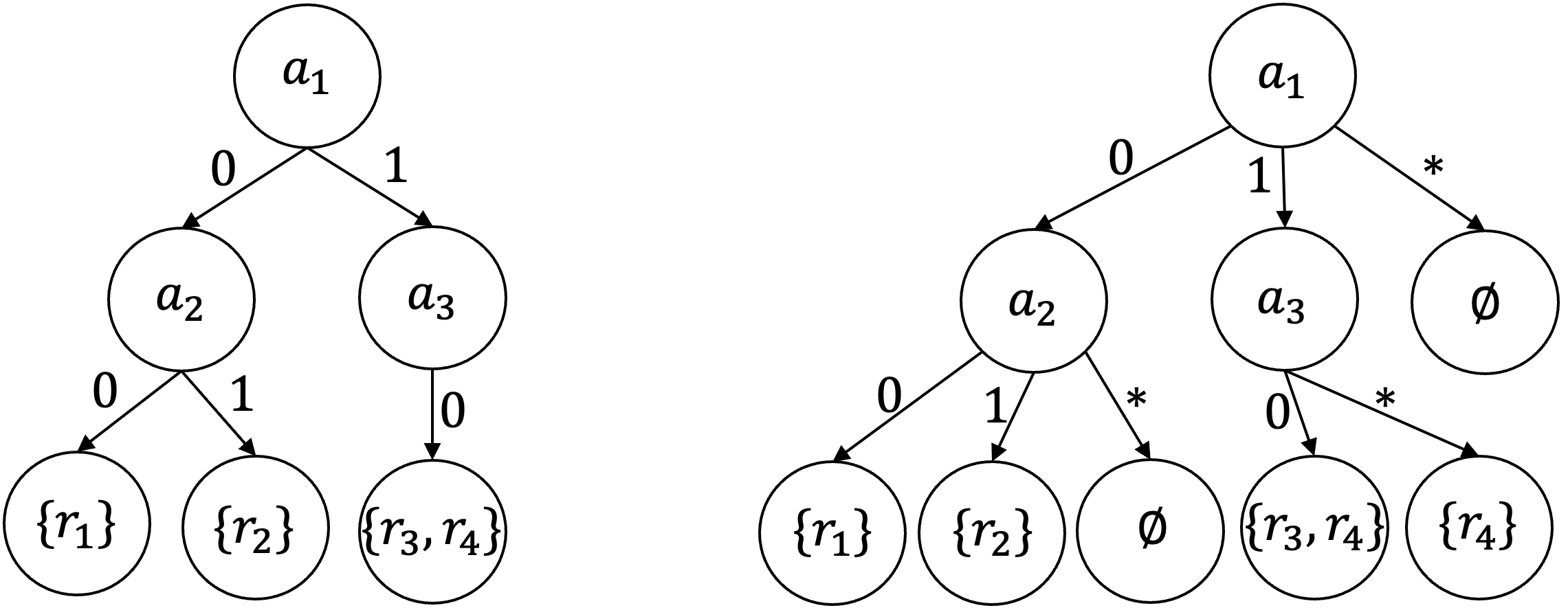
Fig. 1: o-decision tree $\Gamma_{1}$ and e-decision tree $\Gamma_{2}$ over the decision rule system $S$

Let $\xi$ be a complete path in the o-tree $\Gamma_{1}$, which is finished in the terminal node labeled with the set of rules $\{r_{3},r_{4}\}$. Then $A(\xi)=\{a_{1},a_{3}\}$, $K(\xi)=\{a_{1}=1,a_{3}=0\}$ and $\tau(\xi)=\{r_{3},r_{4}\}$.

Definition 11.

A system of equations $\{a_{i_{1}}=\delta_{1},\ldots,a_{i_{m}}=\delta_{m}\}$, where $a_{i_{1}},\ldots,a_{i_{m}}\in A$ and $\delta_{1},\ldots,\delta_{m}\in\omega\cup\{\ast\}$, will be called inconsistent if there exist $l,k\in\{1,\ldots,m\}$ such that $l\neq k$, $i_{l}=i_{k}$, and $\delta_{l}\neq\delta_{k}$. If the system of equations is not inconsistent, then it will be called consistent.

Let $S$ be a decision rule system and $\Gamma$ be a decision tree over $S$.

Definition 12.

We will say that $\Gamma$ solves the problem $AR(S)$ (the problem $EAR(S)$, respectively) if $\Gamma$ is an o-tree (an e-tree, respectively) and any path $\xi\in CP(\Gamma)$ with consistent system of equations $K(\xi)$ satisfies the following conditions:

• For any decision rule $r\in\tau(\xi)$, the relation $K(r)\subseteq K(\xi)$ holds.

• For any decision rule $r\in S\setminus\tau(\xi)$, the system of equations $K(r)\cup K(\xi)$ is inconsistent.

Example 6.

Let $S$ be a decision rule system from Example 4. Then the decision trees $\Gamma_{1}$ and $\Gamma_{2}$ depicted in Fig. 1 solve the problems $AR(S)$ and $EAR(S)$, respectively.

Definition 13.

We will say that $\Gamma$ solves the problem $AD(S)$ (the problem $EAD(S)$, respectively) if $\Gamma$ is an o-tree (an e-tree, respectively) and any path $\xi\in CP(\Gamma)$ with consistent system of equations $K(\xi)$ satisfies the following conditions:

• For any decision rule $r\in\tau(\xi)$, the relation $K(r)\subseteq K(\xi)$ holds.

• If $r\in S\setminus\tau(\xi)$ and the right-hand side of $r$ does not belong to the set $D(\tau(\xi))$, then the system of equations $K(r)\cup K(\xi)$ is inconsistent.

Definition 14.

We will say that $\Gamma$ solves the problem $SR(S)$ (the problem $ESR(S)$, respectively) if $\Gamma$ is an o-tree (an e-tree, respectively) and any path $\xi\in CP(\Gamma)$ with consistent system of equations $K(\xi)$ satisfies the following conditions:

• For any decision rule $r\in\tau(\xi)$, the relation $K(r)\subseteq K(\xi)$ holds.

• If $\tau(\xi)=\emptyset$, then, for any decision rule $r\in S$, the system of equations $K(r)\cup K(\xi)$ is inconsistent.

Example 7.

Let us consider a decision rule system $S=\{(a_{1}=0)\wedge(a_{2}=0)\rightarrow 1,(a_{1}=0)\wedge(a_{2}=1)\rightarrow 2,(a_{1}=1)\wedge(a_{3}=0)\rightarrow 3,(a_{1}=1)\rightarrow 3,(a_{1}=1)\rightarrow 4\}$ and decision trees $\Gamma_{1}$, $\Gamma_{2}$, and $\Gamma_{3}$ depicted in Fig. 2. Then the decision tree $\Gamma_{1}$ solves the problem $AR(S)$, $\Gamma_{2}$ solves $AD(S)$, and $\Gamma_{3}$ solves $SR(S)$, where $r_{1}$, $r_{2}$, $r_{3}$, $r_{4}$ and $r_{5}$ are the first, second, third, fourth and fifth decision rules in $S$, respectively.

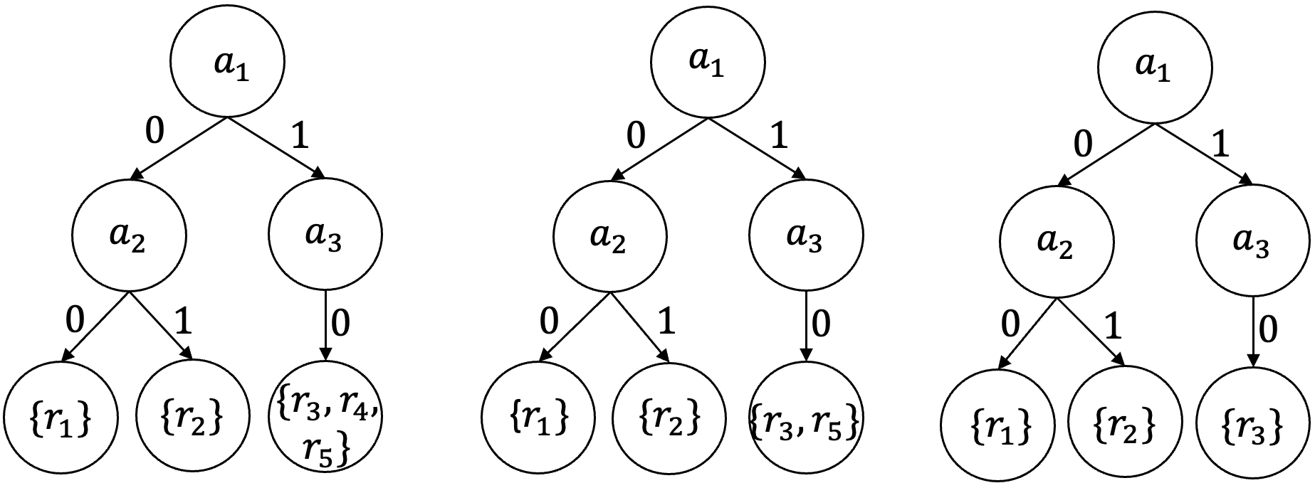
Fig. 2: Decision trees $\Gamma_{1}$, $\Gamma_{2}$, and $\Gamma_{3}$

For any complete path $\xi\in CP(\Gamma)$, we denote by $h(\xi)$ the number of working nodes in $\xi$. The value $h(\Gamma)=\max\{h(\xi):\xi\in CP(\Gamma)\}$ is called the depth of the decision tree $\Gamma$.

Let $S$ be a decision rule system and $C\in\{AR,EAR,AD,EAD,SR,ESR\}$. We denote by $h_{C}(S)$ the minimum depth of a decision tree over $S$, which solves the problem $C(S)$.

Let $n(S)=0$. If $C\in\{AR,EAR\}$, then there is only one decision tree solving the problem $C(S)$. This tree consists of one node labeled with the set of rules $S$. If $C\in\{AD,EAD\}$, then the set of decision trees solving the problem $C(S)$ coincides with the set of trees each of which consists of one node labeled with a subset $Z$ of the set $S$ with $D(Z)=D(S)$. If $C\in\{SR,ESR\}$, then the set of decision trees solving the problem $C(S)$ coincides with the set of trees each of which consists of one node labeled with a nonempty subset $Z$ of the set $S$. Therefore if $n(S)=0$, then $h_{C}(S)=0$ for any $C\in\{AR,EAR,AD,EAD,SR,ESR\}$.

3 Auxiliary Statements

In this section, we will first give some statements from [12] and then we will prove some new ones.

Let $S$ be a decision rule system and $\Gamma$ be an e-decision tree over $S$. We denote by $o(\Gamma)$ an o-tree over $S$, which is obtained from the tree $\Gamma$ by the removal of all nodes $v$ such that the path from the root to the node $v$ in $\Gamma$ contains an edge labeled with $\ast$. Together with a node $v$, we remove all edges entering or leaving $v$.

Lemma 1.

(Lemma 1 [12]) Let $S$ be a decision rule system, $C\in\{AR,AD,SR\}$, and $\Gamma$ be an e-decision tree over $S$ solving the problem $EC(S)$. Then the decision tree $o(\Gamma)$ solves the problem $C(S)$.

Lemma 2.

(Lemma 2 [12]) Let $S$ be a decision rule system and $\Gamma$ be a decision tree over $S$. Then

(a) If the tree $\Gamma$ solves the problem $AR(S)$ ($EAR(S)$, respectively), then the tree $\Gamma$ solves the problem $AD(S)$ ($EAD(S)$, respectively).

(b) If the tree $\Gamma$ solves the problem $AD(S)$ ($EAD(S)$, respectively), then the tree $\Gamma$ solves the problem $SR(S)$ ($ESR(S)$, respectively).

Lemma 3.

(Lemma 3 [12]) Let $S$ be a decision rule system. Then the following inequalities hold:

$$\begin{array}[]{ccccccc}h_{ESR}(S)&\leq&h_{EAD}(S)&\leq&h_{EAR}(S)&\leq&n(S)\\ \mathrel{\rotatebox{90.0}{$\leq$}}&&\mathrel{\rotatebox{90.0}{$\leq$}}&&\mathrel{\rotatebox{90.0}{$\leq$}}&&\\ h_{SR}(S)&\leq&h_{AD}(S)&\leq&h_{AR}(S)&&\end{array}$$

Let $S$ be a decision rule system and $\alpha=\{a_{i_{1}}=\delta_{1},\ldots,a_{i_{m}}=\delta_{m}\}$ be a consistent equation system such that $a_{i_{1}},\ldots,a_{i_{m}}\in A$ and $\delta_{1},\ldots,\delta_{m}\in\omega\cup\{\ast\}$. We now define a decision rule system $S_{\alpha}$. Let $r$ be a decision rule for which the equation system $K(r)\cup\alpha$ is consistent. We denote by $r_{\alpha}$ the decision rule obtained from $r$ by the removal from the left-hand side of $r$ all equations that belong to $\alpha$. Then $S_{\alpha}$ is the set of decision rules $r_{\alpha}$ such that $r\in S$ and the equation system $K(r)\cup\alpha$ is consistent.

Lemma 4.

(Lemma 6 [12]) Let $S$ be a decision rule system with $n(S)>0$, $C\in\{EAR,AR,\\ EAD,AD,ESR,$ $SR\}$, $\alpha=\{a_{i_{1}}=\delta_{1},\ldots,a_{i_{m}}=\delta_{m}\}$ be a consistent equation system such that $a_{i_{1}},\ldots,a_{i_{m}}\in A(S)$ and, for $j=1,\ldots,m$, $\delta_{j}\in EV_{S}(a_{i_{j}})$ if $C\in\{EAR,EAD,ESR\}$ and $\delta_{j}\in V_{S}(a_{i_{j}})$ if $C\in\{AR,AD,SR\}$. Then $h_{C}(S)\geq h_{C}(S_{\alpha})$.

We correspond to a decision rule system $S$ a hypergraph $G(S)$ with the set of nodes $A(S)$ and the set of edges $\{A(r):r\in S\}$. A node cover of the hypergraph $G(S)$ is a subset $B$ of the set of nodes $A(S)$ such that $A(r)\cap B\neq\emptyset$ for any rule $r\in S$ such that $A(r)\neq\emptyset$. If $A(S)=\emptyset$, then the empty set is the only node cover of the hypergraph $G(S)$. Denote by $\beta(S)$ the minimum cardinality of a node cover of the hypergraph $G(S)$.

Example 8.

Let us consider a decision rule system $S=\{(a_{1}=0)\wedge(a_{2}=1)\rightarrow 1,(a_{1}=0)\wedge(a_{3}=1)\rightarrow 2,(a_{4}=0)\rightarrow 3\}$. One can show, that the set $\{a_{1},a_{4}\}$ is a node cover of the hypergraph $G(S)$ and $\beta(S)=2$.

We define a subsystem $I_{SR}(S)$ of the system $S$ in the following way. If $S$ does not contain rules of the length $0$, then $I_{SR}(S)=S$. Otherwise, $I_{SR}(S)$ consists of all rules from $S$ of the length $0$.

Remark 1.

Note that $I_{SR}(S)\neq S$ if and only if $S$ contains both a rule of the length $0$ and a rule of the length greater than $0$.

We now define a subsystem $I_{AD}(S)$ of the system $S$. Denote by $D_{0}(S)$ the set of the right-hand sides of decision rules from $S$, which length is equal to $0$. Then the subsystem $I_{AD}(S)$ consists of all rules from $S$ of the length $0$ and all rules from $S$ for which the right-hand sides do not belong to $D_{0}(S)$.

Remark 2.

Note that $I_{AD}(S)\neq S$ if and only if $S$ contains both a rule of the length $0$ and a rule of the length greater than $0$ with the same right-hand sides.

Example 9.

Let us consider a decision rule system $S=\{(a_{1}=0)\rightarrow 1,(a_{2}=0)\rightarrow 2,\rightarrow 2\}$. For this system, $I_{SR}(S)=\{\rightarrow 2\}$ and $I_{AD}(S)=\{(a_{1}=0)\rightarrow 1,\rightarrow 2\}$.

Let $S$ be a decision rule system. This system will be called incomplete if there exists a tuple $\bar{\delta}\in V(S)$ such that the equation system $K(r)\cup K(S,\bar{\delta})$ is inconsistent for any decision rule $r\in S$. Otherwise, the system $S$ will be called complete. If $n(S)=0$, then the system $S$ will be considered as complete.

Lemma 5.

(Lemma 7 [12]) Let $S$ be a decision rule system. Then

(a) If $C\in\{EAR,AR\}$, then $h_{C}(S)\geq\beta(S)$.

(b) If $C\in\{AD,SR\}$, then $h_{EC}(S)\geq\beta(I_{C}(S))$.

(c) If $C\in\{AD,SR\}$ and the system $S$ is incomplete, then $h_{C}(S)\geq\beta(S)$.

Lemma 6.

(Lemma 8 [12]) Let $S$ be a decision rule system. Then

(a) $h_{EAR}(S)\geq h_{AR}(S)\geq d(S)$.

(b) If $S$ is an $SR$-reduced system, then $h_{ESR}(S)\geq d(S)$.

(c) If $S$ is an $AD$-reduced system, then $h_{EAD}(S)\geq d(S)$.

Lemma 7.

(Lemma 9 [12]) Let $S$ be a decision rule system. Then $h_{ESR}(S)=h_{ESR}(R_{SR}(S))$ and $h_{EAD}(S)=h_{EAD}(R_{AD}(S))$.

Let $C\in\{AR,EAR,AD,EAD,SR,ESR\}$, $S$ be a decision rule system, and $\Gamma$ be a decision tree over $S$. We denote by $L(\Gamma)$ the number of nodes in the tree $\Gamma$ and by $T(\Gamma)$ we denote the number of terminal nodes in $\Gamma$ that are labeled with pairwise different sets of decision rules. Let $L_{C}(S)=\min L(\Gamma)$ and $T_{C}(S)=\min T(\Gamma)$, where the minimum is taken over all decision trees $\Gamma$ over $S$ that solve the problem $C(S)$. It is clear that $T_{C}(S)\leq L_{C}(S)$.

Lemma 8.

Let $S$ be a decision rule system. Then the following inequalities hold:

$\begin{array}[]{ccccc}L_{ESR}(S)&\leq&L_{EAD}(S)&\leq&L_{EAR}(S)\\ \mathrel{\rotatebox{90.0}{$\leq$}}&&\mathrel{\rotatebox{90.0}{$\leq$}}&&\mathrel{\rotatebox{90.0}{$\leq$}}\\ L_{SR}(S)&\leq&L_{AD}(S)&\leq&L_{AR}(S),\end{array}$ $\begin{array}[]{ccccc}T_{ESR}(S)&\leq&T_{EAD}(S)&\leq&T_{EAR}(S)\\ \mathrel{\rotatebox{90.0}{$\leq$}}&&\mathrel{\rotatebox{90.0}{$\leq$}}&&\mathrel{\rotatebox{90.0}{$\leq$}}\\ T_{SR}(S)&\leq&T_{AD}(S)&\leq&T_{AR}(S).\end{array}$

Proof.

It is clear that the considered inequalities hold if $n(S)=0$. Let $n(S)>0$.

Let $\Gamma$ be an e-decision tree over $S$. It is clear that $L(o(\Gamma))\leq L(\Gamma)$ and $T(o(\Gamma))\leq T(\Gamma)$. Using these inequalities and Lemma 1, we obtain that $L_{SR}(S)\leq L_{ESR}(S)$, $L_{AD}(S)\leq L_{EAD}(S)$, $L_{AR}(S)\leq L_{EAR}(S)$, $T_{SR}(S)\leq T_{ESR}(S)$, $T_{AD}(S)\leq T_{EAD}(S)$, and $T_{AR}(S)\leq T_{EAR}(S)$.

Using Lemma 2, we obtain that $L_{ESR}(S)\leq L_{EAD}(S)\leq L_{EAR}(S)$, $L_{SR}(S)\leq L_{AD}(S)\leq L_{AR}(S)$, $T_{ESR}(S)\leq T_{EAD}(S)\leq T_{EAR}(S)$, and $T_{SR}(S)\leq T_{AD}(S)\leq T_{AR}(S)$. ∎

A system of decision rules $S$ can be represented by a word over the alphabet

$$\{(,),a,=,\wedge,\rightarrow,0,1,;\}$$

in which numbers from $\omega$ (attribute indexes, attribute values, and right-hand sides of decision rules) are in binary representation (are represented by words over the alphabet $\{0,1\}$) and the symbol “;” is used to separate two rules. The length of this word will be called the size of the decision rule system $S$ and will be denoted $size(S)$.

Definition 15.

A decision rule system $S$ will be called reduced if it satisfies the following conditions:

• If $n(s)=n$, then $A(S)\subseteq\{a_{0},\ldots,a_{n}\}$.

• If $\left|D(S)\right|=t$, then $D(S)\subseteq\{0,\ldots,t\}$.

• If $k(S)=k$, then $V_{S}(a_{i})\subseteq\{0,\ldots,k\}$ for any $a_{i}\in A(S)$.

• $d(S)\geq 1$.

Let $S$ be a reduced system of decision rules. It is clear that $n(S)\leq d(S)\left|S\right|$, $k(S)\leq\left|S\right|$, and $\left|D(S)\right|\leq\left|S\right|$. Therefore the maximum number from $\omega$ in the system $S$ is at most $d(S)\left|S\right|$. The length of binary representation of such a number is at most $\log_{2}(d(S)\left|S\right|)+1$. The length of each rule from $S$ is at most $d(S)$. One can show that the length of word representing each rule (including the sign “;” after it) is at most $10d(S)(\log_{2}(d(S)\left|S\right|)+1)$ and

$$size(S)\leq 10\left|S\right|d(S)(\log_{2}(d(S)\left|S\right|)+1).$$ (1)

Lemma 9.

Let $n,k,d\in\omega\setminus\{0\}$, $d\geq 2$, and $k\geq 2$. Then there exists a reduced decision rule system $S$ such that $n(S)=2n+d$, $k(S)=k$, $d(S)=d$, $\left|S\right|=2n+k-1$, and $L_{SR}(S)\geq 2^{n}$.

Proof.

Let us consider a system of decision rules $S=S_{1}\cup S_{2}\cup S_{3}$, where $S_{1}=\{(a_{2i-1}=0)\wedge(a_{2i}=0)\rightarrow 0,(a_{2i-1}=1)\wedge(a_{2i}=1)\rightarrow 0:i=1,\ldots,n\}$, $S_{2}=\{(a_{1}=2)\wedge(a_{2}=2)\rightarrow 0,\ldots,(a_{1}=k-1)\wedge(a_{2}=k-1)\rightarrow 0\}$, and $S_{3}=\{(a_{2n+1}=0)\wedge\cdots\wedge(a_{2n+d}=0)\rightarrow 0\}$. If $k=2$, then $S_{2}=\emptyset$. It is clear that $S$ is reduced, $n(S)=2n+d$, $k(S)=k$, $d(S)=d$, and $\left|S\right|=2n+k-1$. Denote by $\Delta$ the set of tuples $(\delta_{1},\ldots,\delta_{2n+d})\in\{0,1\}^{2n+d}$ such that $\delta_{2i-1}+\delta_{2i}=1$ for $i=1,\ldots,n$ and $\delta_{2n+1}=\cdots=\delta_{2n+d}=1$. It is clear that $\left|\Delta\right|=2^{n}$ and, for any $\bar{\delta}\in\Delta$, there is no a rule from $S$ that is realizable for the tuple $\bar{\delta}$.

Let $\Gamma$ be a decision tree over $S$, which solves the problem $SR(S)$ and for which $L(\Gamma)=L_{SR}(S)$. Let $\bar{\delta}=(\delta_{1},\ldots,\delta_{2n+d})\in\Delta$. It is clear that there exists a complete path $\xi$ in $\Gamma$ such that $K(\xi)\subseteq K(S,\bar{\delta})$. Evidently, the terminal node of this path is labeled with the empty set. Let us show that $\{a_{1}=\delta_{1},\ldots,a_{2n}=\delta_{2n}\}\subseteq K(\xi)$. Let us assume the contrary. Then there exists $j\in\{1,\ldots,2n\}$ such that the equation $a_{j}=\delta_{j}$ does not belong to $K(\xi)$. Let $j\in\{2i-1,2i\}$, where $i\in\{1,\ldots,n\}$. Denote by $r_{0}$ the rule $(a_{2i-1}=0)\wedge(a_{2i}=0)\rightarrow 0$ and by $r_{1}$ – the rule $(a_{2i-1}=1)\wedge(a_{2i}=1)\rightarrow 0$. It is clear that $r_{0},r_{1}\in S$ and at least one of the equation systems $K(r_{0})\cup K(\xi)$ and $K(r_{1})\cup K(\xi)$ is consistent but this is impossible. Therefore $\{a_{1}=\delta_{1},\ldots,a_{2n}=\delta_{2n}\}\subseteq K(\xi)$. From this relation and the inclusion $K(\xi)\subseteq K(S,\bar{\delta})$ it follows that in $\Gamma$ there are at least $2^{n}$ pairwise different complete paths. Therefore $L(\Gamma)\geq 2^{n}$ and $L_{SR}(S)\geq 2^{n}$. ∎

Lemma 10.

Let $n,d\in\omega\setminus\{0\}$ and $d\geq 2$. Then there exists a reduced decision rule system $S$ such that $n(S)=2n+d$, $k(S)=1$, $d(S)=d$, $\left|S\right|=n+1$, and $L_{ESR}(S)\geq 2^{n}$.

Proof.

Let us consider a system of decision rules $S=S_{1}\cup S_{2}$, where $S_{1}=\{(a_{2i-1}=0)\wedge(a_{2i}=0)\rightarrow 0:i=1,\ldots,n\}$ and $S_{2}=\{(a_{2n+1}=0)\wedge\cdots\wedge(a_{2n+d}=0)\rightarrow 0\}$. It is clear that $S$ is reduced, $n(S)=2n+d$, $d(S)=d$, $k(S)=1$, and $\left|S\right|=n+1$. Denote by $\Delta$ the set of tuples $(\delta_{1},\ldots,\delta_{2n+d})\in\{0,\ast\}^{2n+d}$ such that $\{\delta_{2i-1},\delta_{2i}\}=\{0,\ast\}$ for $i=1,\ldots,n$ and $\delta_{2n+1}=\cdots=\delta_{2n+d}=\ast$. It is clear that $\left|\Delta\right|=2^{n}$ and, for any $\bar{\delta}\in\Delta$, there is no a rule from $S$ that is realizable for the tuple $\bar{\delta}$. Let $\Gamma$ be a decision tree over $S$, which solves the problem $ESR(S)$ and for which $L(\Gamma)=L_{ESR}(S)$. Let $\bar{\delta},\bar{\sigma}\in\Delta$ and $\bar{\delta}\neq\bar{\sigma}$. It is clear that there exist complete paths $\xi,\tau$ in $\Gamma$ such that $K(\xi)\subseteq K(S,\bar{\delta})$ and $K(\tau)\subseteq K(S,\bar{\sigma})$. Let us show that $\xi\neq\tau$. Let us assume the contrary: $\xi=\tau$. It is clear that the terminal node of the path $\xi$ is labeled with the empty set. Since $\bar{\delta}\neq\bar{\sigma}$, there exists $i\in\{1,\ldots,n\}$ such that $(2i-1)$th and $(2i)$th digits of the tuples $\bar{\delta}$ and $\bar{\sigma}$ are different. Therefore the attributes $a_{2i-1}$ and $a_{2i}$ are not attached to any node of the path $\xi$. Hence the system of equations $K(r)\cup K(\xi)$ is consistent, where $r$ is the rule $(a_{2i-1}=0)\wedge(a_{2i}=0)\rightarrow 0$ from $S$, but this is impossible. Therefore $\xi\neq\tau$. Thus, in the tree $\Gamma$, there are at least $2^{n}$ pairwise different complete paths. As a result, we have $L(\Gamma)\geq 2^{n}$ and $L_{ESR}(S)\geq 2^{n}$. ∎

Lemma 11.

(a) Let $n,d\in\omega\setminus\{0\}$. Then there exists a reduced decision rule system $S$ such that $n(S)=n+d$, $k(S)=1$, $d(S)=d$, $\left|S\right|=n+1$, and $T_{EAD}(S)\geq 2^{n+1}$.

(b) Let $n,d,k\in\omega\setminus\{0\}$ and $k\geq 2$. Then there exists a reduced decision rule system $S$ such that $n(S)=n+d$, $k(S)=k$, $d(S)=d$, $\left|S\right|=2n+k-1$, and $T_{AD}(S)\geq 2^{n}$.

Proof.

(a) Let us consider a system of decision rules $S=\{(a_{1}=0)\rightarrow 1,(a_{2}=0)\rightarrow 2,\ldots,(a_{n}=0)\rightarrow n,(a_{n+1}=0)\wedge\cdots\wedge(a_{n+d}=0)\rightarrow n+1\}$. It is clear that $S$ is reduced, $n(S)=n+d$, $k(S)=1$, $d(S)=d$, $\left|S\right|=n+1$, and the problem $EAD(S)$ has $2^{n+1}$ pairwise different solutions. Therefore any decision tree solving the problem $EAD(S)$ has at least $2^{n+1}$ terminal nodes that are labeled with pairwise different sets of decision rules. Hence $T_{EAD}(S)\geq 2^{n+1}$.

(b) Let us consider a decision rule system $S=S_{1}\cup S_{2}\cup S_{3}$, where $S_{1}=\{(a_{i}=0)\rightarrow 2i-1,(a_{i}=1)\rightarrow 2i:i=1,\ldots,n\}$, $S_{2}=\{(a_{n+1}=0)\wedge\cdots\wedge(a_{n+d}=0)\rightarrow 0\}$, and $S_{3}=\{(a_{1}=2)\rightarrow 0,\ldots,(a_{1}=k-1)\rightarrow 0\}$. If $k=2$, then $S_{3}=0$. It is clear that $S$ is reduced, $n(S)=n+d$, $k(S)=k$, $d(S)=d$, and $\left|S\right|=2n+k-1$. It is also clear that the problem $AD(S)$ has at least $2^{n}$ pairwise different solutions. Therefore any decision tree solving the problem $AD(S)$ has at least $2^{n}$ terminal nodes that are labeled with pairwise different sets of decision rules. Hence $T_{AD}(S)\geq 2^{n}$. ∎

Let $k,d\in\omega\setminus\{0\}$. Denote $\Sigma(k,d)=\{S\in\Sigma:k(S)=k,d(S)=d\}$. We will consider only sequential algorithms for the construction of decision trees and will evaluate their time complexity depending on the size of decision rule systems on the algorithm input.

Lemma 12.

Let $d\in\omega\setminus\{0\}$ and $C\in\{SR,AD,AR\}$. Then there exists a polynomial time algorithm that, for a given decision rule system $S\in\Sigma(1,d)$, constructs a decision tree solving the problem $C(S)$.

Proof.

Let $S\in\Sigma(1,d)$, $A(S)=\{a_{i_{1}},\ldots,a_{i_{m}}\}$, $i_{1}<\cdots<i_{m}$, and $V(S)=\{(\delta_{1},\ldots,\delta_{m})\}$. We construct a decision tree $\Gamma$ that consists of one complete path $\xi=v_{1},d_{1},\ldots,v_{m},d_{m},v_{m+1}$ such that, for $j=1,\ldots,m$, the node $v_{j}$ is labeled with the attribute $a_{i_{j}}$, the edge $d_{j}$ is labeled with the number $\delta_{j}$, and the node $v_{m+1}$ is labeled with the set of decision rules $S$. It is clear that $\Gamma$ solves the problem $C(S)$ and the considered algorithm has polynomial time complexity. ∎

Lemma 13.

Let $k\in\omega\setminus\{0\}$ and $C\in\{SR,ESR\}$. Then there exists a polynomial time algorithm that, for a given decision rule system $S\in\Sigma(k,1)$, constructs a decision tree solving the problem $C(S)$.

Proof.

Let $S\in\Sigma(k,1)$ and $S$ contain a rule $r$ of the length $0$. Construct a decision tree $\Gamma_{0}$ that contains only one node labeled with the set $\{r\}$. It is clear that $\Gamma_{0}$ solves the problem $C(S)$ and the considered algorithm has polynomial time complexity.

Let us assume now that $S$ does not contain rules of the length $0$ and $A(S)=\{a_{i_{1}},\ldots,a_{i_{n}}\}$. Let $j\in\{1,\ldots,n\}$ and $\delta\in V_{S}(a_{i_{j}})$. It is clear that in the system $S$ there exists a decision rule for which the left-hand side is equal to $a_{i_{j}}=\delta$. Denote this rule by $r(j,\delta)$.

Let us construct a decision tree $\Gamma_{1}$. Let $V_{S}(a_{i_{1}})=\{\delta_{1},\ldots,\delta_{m}\}$. The decision tree $\Gamma_{1}$ consists of the nodes $v_{0},v_{1},\ldots,v_{m}$ and the edges $d_{1},\ldots,d_{m}$. The node $v_{0}$ is labeled with the attribute $a_{i_{1}}$, and the node $v_{j}$ is labeled with the set $\{r(1,\delta_{j})\}$, $j=1,\ldots,m$. For $j=1,\ldots,m$, the edge $d_{j}$ is labeled with the number $\delta_{j}$, the edge $d_{j}$ leaves the node $v_{0}$ and enters the node $v_{j}$. It is clear that $\Gamma_{1}$ solves the problem $SR(S)$ and the considered algorithm has polynomial time complexity.

Let us construct a decision tree $\Gamma_{2}$. The tree $\Gamma_{2}$ contains a complete path $\xi=v_{1},d_{1},\ldots,$ $v_{n},d_{n},v_{n+1}$. For $j=1,\ldots,n$, the node $v_{j}$ is labeled with the attribute $a_{i_{j}}$ and the edge $d_{j}$ is labeled with the symbol $\ast$. The node $v_{n+1}$ is labeled with the empty set. Let $j\in\{1,\ldots,n\}$ and $V_{S}(a_{i_{j}})=\{\delta_{1},\ldots,\delta_{m}\}$. Besides the edge $d_{j}$, also the edges $d_{j1},\ldots,d_{jm}$ leave the node $v_{j}$. These edges are labeled with the numbers $\delta_{1},\ldots,\delta_{m}$, respectively. The edges $d_{j1},\ldots,d_{jm}$ enter the nodes $v_{j1},\ldots,v_{jm}$ that are labeled with the sets $\{r(j,\delta_{1})\},\ldots,\{r(j,\delta_{m})\}$, respectively. The tree $\Gamma$ does not contain any other nodes and edges. It is clear that $\Gamma_{2}$ solves the problem $ESR(S)$ and the considered algorithm has polynomial time complexity. ∎

4 Construction of Decision Trees

As it was mentioned above, we consider only sequential algorithms for the construction of decision trees and evaluate their time complexity depending on the size of decision rule systems on the algorithm input. We assume that, during each unit of time, the algorithm can add to the constructing decision tree at most one node.

Let $C\in\{SR,ESR,AD,EAD,AR,EAR\}$. Denote by $P_{DT}(C)$ the set of pairs $(k,d)\in(\omega\setminus\{0\})^{2}$ satisfying the following condition: there exists a polynomial time algorithm that, for an arbitrary decision rule system $S\in\Sigma(k,d)$, constructs a decision tree solving the problem $C(S)$.

Theorem 1.

(a) $P_{DT}(ESR)=\{(k,1):k\in\omega\setminus\{0\}\}$, (b) $P_{DT}(SR)=\{(k,1),(1,d):k,d\in\omega\setminus\{0\}\}$, (c) $P_{DT}(EAD)=P_{DT}(EAR)=\emptyset$, and (d) $P_{DT}(AD)=P_{DT}(AR)=\{(1,d):d\in\omega\setminus\{0\}\}$.

Proof.

Let $C\in\{SR,ESR,AD,EAD,AR,EAR\}$, $(k,d)\in(\omega\setminus\{0\})^{2}$ and let us assume that there exists a polynomial time algorithm, which, for a given decision rule system $S\in\Sigma(k,d)$, constructs a decision tree solving the problem $C(S)$. Then there exists a polynomial $\pi$ such that, for any $S\in\Sigma(k,d)$, $L_{C}(S)\leq\pi(size(S))$. If $S$ is reduced, then, by (1), $size(S)\leq 10\left|S\right|d(S)(\log_{2}(d(S)\left|S\right|)+1)$. We know that, for systems $S\in\Sigma(k,d)$, $d(S)\leq d$. Therefore there exists a polynomial $\varrho$ such that $L_{C}(S)\leq\varrho(\left|S\right|)$ for any reduced system $S\in\Sigma(k,d)$.

(a) Using Lemma 13, we obtain that $\{(k,1):k\in\omega\setminus\{0\}\}\subseteq P_{DT}(ESR)$. Let $k,d\in\omega\setminus\{0\}$ and $d>1$. We now show that $(k,d)\notin P_{DT}(ESR)$. Let us assume the contrary: $(k,d)\in P_{DT}(ESR)$. Then there exists a polynomial $\varrho$ such that $L_{ESR}(S)\leq\varrho(\left|S\right|)$ for any reduced system $S\in\Sigma(k,d)$. Let $k=1$. Using Lemma 10, we obtain that, for any $n\in\omega\setminus\{0\}$, there exists a reduced decision rule system $S\in\Sigma(k,d)$ such that $\left|S\right|=n+1$ and $L_{ESR}(S)\geq 2^{n}$. Therefore $2^{n}\leq\varrho(n+1)$ for any $n\in\omega\setminus\{0\}$ but this is impossible. Let $k>1$. Using Lemma 9, we obtain that, for any $n\in\omega\setminus\{0\}$, there exists a reduced decision rule system $S\in\Sigma(k,d)$ such that $\left|S\right|=2n+k-1$ and $L_{SR}(S)\geq 2^{n}$. By Lemma 8, $L_{ESR}(S)\geq 2^{n}$. Therefore, $2^{n}\leq\varrho(2n+k-1)$ for any $n\in\omega\setminus\{0\}$ but this is impossible since $k$ is a constant for the considered systems of decision rules. Hence $(k,d)\notin P_{DT}(ESR)$ if $d>1$. Thus, $P_{DT}(ESR)=\{(k,1):k\in\omega\setminus\{0\}\}$.

(b) Using Lemmas 12 and 13, we obtain that $\{(k,1),(1,d):k,d\in\omega\setminus\{0\}\}\subseteq P_{DT}(SR)$. Let $k,d\in\omega\setminus\{0,1\}$. We now show that $(k,d)\notin P_{DT}(SR)$. Let us assume the contrary: $(k,d)\in P_{DT}(SR)$. Then there exists a polynomial $\varrho$ such that $L_{SR}(S)\leq\varrho(\left|S\right|)$ for any reduced system $S\in\Sigma(k,d)$. Using Lemma 9, we obtain that, for any $n\in\omega\setminus\{0\}$, there exists a reduced decision rule system $S\in\Sigma(k,d)$ such that $\left|S\right|=2n+k-1$ and $L_{SR}(S)\geq 2^{n}$. Therefore, $2^{n}\leq\varrho(2n+k-1)$ for any $n\in\omega\setminus\{0\}$ but this is impossible since $k$ is a constant for the considered systems of decision rules. Hence $(k,d)\notin P_{DT}(SR)$ if $k>1$ and $d>1$. Thus, $P_{DT}(SR)=\{(k,1),(1,d):k,d\in\omega\setminus\{0\}\}$.

(c) Let $k,d\in\omega\setminus\{0\}$. We now show that $(k,d)\notin P_{DT}(EAD)$. Let us assume the contrary: $(k,d)\in P_{DT}(EAD)$. Then there exists a polynomial $\varrho$ such that $L_{EAD}(S)\leq\varrho(\left|S\right|)$ for any reduced system $S\in\Sigma(k,d)$. Let $k=1$. Using Lemma 11, we obtain that, for any $n\in\omega\setminus\{0\}$, there exists a reduced decision rule system $S\in\Sigma(k,d)$ such that $\left|S\right|=n+1$ and $T_{EAD}(S)\geq 2^{n+1}$. It is clear that $L_{EAD}(S)\geq T_{EAD}(S)$ and $L_{EAD}(S)\geq 2^{n+1}$. Therefore, $2^{n+1}\leq\varrho(n+1)$ for any $n\in\omega\setminus\{0\}$ but this is impossible. Let $k>1$. Using Lemma 11, we obtain that, for any $n\in\omega\setminus\{0\}$, there exists a reduced decision rule system $S\in\Sigma(k,d)$ such that $\left|S\right|=2n+k-1$ and $T_{AD}(S)\geq 2^{n}$. By Lemma 8, $T_{EAD}(S)\geq T_{AD}(S)$. It is clear that $L_{EAD}(S)\geq T_{EAD}(S)$ and $L_{EAD}(S)\geq 2^{n}$. Therefore, $2^{n}\leq\varrho(2n+k-1)$ for any $n\in\omega\setminus\{0\}$ but this is impossible since $k$ is a constant for the considered systems of decision rules. Hence $(k,d)\notin P_{DT}(EAD)$. Thus, $P_{DT}(EAD)=\emptyset$.

Let $k,d\in\omega\setminus\{0\}$. We now show that $(k,d)\notin P_{DT}(EAR)$. Let us assume the contrary: $(k,d)\in P_{DT}(EAR)$. Then there exists a polynomial $\varrho$ such that $L_{EAR}(S)\leq\varrho(\left|S\right|)$ for any reduced system $S\in\Sigma(k,d)$. Let $k=1$. Using Lemma 11, we obtain that, for any $n\in\omega\setminus\{0\}$, there exists a reduced decision rule system $S\in\Sigma(k,d)$ such that $\left|S\right|=n+1$ and $T_{EAD}(S)\geq 2^{n+1}$. It is clear that $L_{EAD}(S)\geq T_{EAD}(S)$. By Lemma 8, $L_{EAR}(S)\geq L_{EAD}(S)$ and $L_{EAR}(S)\geq 2^{n+1}$. Therefore, $2^{n+1}\leq\varrho(n+1)$ for any $n\in\omega\setminus\{0\}$ but this is impossible. Let $k>1$. Using Lemma 11, we obtain that, for any $n\in\omega\setminus\{0\}$, there exists a reduced decision rule system $S\in\Sigma(k,d)$ such that $\left|S\right|=2n+k-1$ and $T_{AD}(S)\geq 2^{n}$. By Lemma 8, $T_{EAR}(S)\geq T_{AD}(S)$. It is clear that $L_{EAR}(S)\geq T_{EAR}(S)$ and $L_{EAR}(S)\geq 2^{n}$. Therefore, $2^{n}\leq\varrho(2n+k-1)$ for any $n\in\omega\setminus\{0\}$ but this is impossible since $k$ is a constant for the considered systems of decision rules. Hence $(k,d)\notin P_{DT}(EAR)$. Thus, $P_{DT}(EAR)=\emptyset$.

(d) Using Lemma 12, we obtain that $\{(1,d):d\in\omega\setminus\{0\}\}\subseteq P_{DT}(AD)$ and $\{(1,d):d\in\omega\setminus\{0\}\}\subseteq P_{DT}(AR)$ .

Let $k,d\in\omega\setminus\{0\}$ and $k\geq 2$. We now show that $(k,d)\notin P_{DT}(AD)$. Let us assume the contrary: $(k,d)\in P_{DT}(AD)$. Then there exists a polynomial $\varrho$ such that $L_{AD}(S)\leq\varrho(\left|S\right|)$ for any reduced system $S\in\Sigma(k,d)$. Using Lemma 11, we obtain that, for any $n\in\omega\setminus\{0\}$, there exists a reduced decision rule system $S\in\Sigma(k,d)$ such that $\left|S\right|=2n+k-1$ and $T_{AD}(S)\geq 2^{n}$. It is clear that $L_{AD}(S)\geq T_{AD}(S)$ and $L_{AD}(S)\geq 2^{n}$. Therefore, $2^{n}\leq\varrho(2n+k-1)$ for any $n\in\omega\setminus\{0\}$ but this is impossible since $k$ is a constant for the considered systems of decision rules. Hence $(k,d)\notin P_{DT}(AD)$. Thus, $P_{DT}(AD)=\{(1,d):d\in\omega\setminus\{0\}\}$.

Let $k,d\in\omega\setminus\{0\}$ and $k\geq 2$. We now show that $(k,d)\notin P_{DT}(AR)$. Let us assume the contrary: $(k,d)\in P_{DT}(AR)$. Then there exists a polynomial $\varrho$ such that $L_{AR}(S)\leq\varrho(\left|S\right|)$ for any reduced system $S\in\Sigma(k,d)$. Using Lemma 11, we obtain that, for any $n\in\omega\setminus\{0\}$, there exists a reduced decision rule system $S\in\Sigma(k,d)$ such that $\left|S\right|=2n+k-1$ and $T_{AD}(S)\geq 2^{n}$. It is clear that $L_{AD}(S)\geq T_{AD}(S)$. By Lemma 8, $L_{AR}(S)\geq L_{AD}(S)$ and $L_{AR}(S)\geq 2^{n}$. Therefore, $2^{n}\leq\varrho(2n+k-1)$ for any $n\in\omega\setminus\{0\}$ but this is impossible since $k$ is a constant for the considered systems of decision rules. Hence $(k,d)\notin P_{DT}(AR)$. Thus, $P_{DT}(AR)=\{(1,d):d\in\omega\setminus\{0\}\}$. ∎

5 Construction of Acyclic Decision Graphs

Besides decision trees, we will also consider acyclic decision graphs that are defined similarly to the decision trees, but instead of finite directed trees with roots, finite directed graphs with roots that do not have directed cycles are considered. Note that any decision tree is an acyclic decision graph. Let $C\in\{SR,ESR,AD,EAD,AR,EAR\}$. For a decision rule system $S$, we denote by $L^{DG}_{C}(S)$ the minimum number of nodes in an acyclic decision graph, which solves the problem $C(S)$. One can show that $L^{DG}_{C}(S)\geq T_{C}(S)$.

First, we describe a construction that will be used in this and in the next section. Let $C\in\{SR,ESR,AD,EAD,AR,EAR\}$, $S\in\Sigma$, and $r\in S$ be a decision rule of the form $(a_{i_{1}}=\delta_{1})\wedge\cdots\wedge(a_{i_{m}}=\delta_{m})\rightarrow\sigma$, where $m>0$. For $j=1,\ldots,m$, let $V_{S}^{C}(a_{i_{j}})=V_{S}(a_{i_{j}})$ if $C\in\{SR,AD,AR\}$ and $V_{S}^{C}(a_{i_{j}})=EV_{S}(a_{i_{j}})$ if $C\in\{ESR,EAD,EAR\}$. We now describe an acyclic decision graph $G_{S}^{C}(r)$. The graph $G_{S}^{C}(r)$ contains $m+2$ nodes $v_{1},\ldots,v_{m},v_{m+1},v_{m+2}$. The node $v_{1}$ is the root of $G_{S}^{C}(r)$. For $j=1,\ldots,m$, the node $v_{j}$ is labeled with the attribute $a_{i_{j}}$, the node $v_{m+1}$ is labeled with the set $\{r\}$, and the node $v_{m+2}$ is labeled with the empty set. For $j=1,\ldots,m$, exactly $\left|V_{S}^{C}(a_{i_{j}})\right|$ edges leave the node $v_{j}$. These edges are labeled with pairwise different elements from the set $V_{S}^{C}(a_{i_{j}})$. The edge labeled with the number $\delta_{j}$ enters the node $v_{j+1}$. All other edges enter the node $v_{m+2}$. The graph $G_{S}^{C}(r)$ does not contain other nodes and edges.

We consider only sequential algorithms for the construction of acyclic decision graphs and evaluate their time complexity depending on the size of decision rule systems on the algorithm input. We assume that, during each unit of time, the algorithm can add to the constructing acyclic decision graph at most one node.

Let $C\in\{SR,ESR,AD,EAD,AR,EAR\}$. Denote by $P_{DG}(C)$ the set of pairs $(k,d)\in(\omega\setminus\{0\})^{2}$ satisfying the following condition: there exists a polynomial time algorithm that, for an arbitrary decision rule system $S\in\Sigma(k,d)$, constructs an acyclic decision graph solving the problem $C(S)$.

Theorem 2.

(a) $P_{DG}(SR)=P_{DG}(ESR)=(\omega\setminus\{0\})^{2}$, (b) $P_{DG}(AD)=P_{DG}(AR)=\{(1,d):d\in\omega\setminus\{0\}\}$, and (c) $P_{DG}(EAD)=P_{DG}(EAR)=\emptyset$.

Proof.

Let $C\in\{SR,ESR,AD,EAD,AR,EAR\}$ and $(k,d)\in(\omega\setminus\{0\})^{2}$. Let us assume that there exists a polynomial time algorithm, which, for a given decision rule system $S\in\Sigma(k,d)$, constructs an acyclic decision graph solving the problem $C(S)$. Then there exists a polynomial $\pi$ such that, for any $S\in\Sigma(k,d)$, $L^{DG}_{C}(S)\leq\pi(size(S))$. If $S$ is reduced, then, by (1), $size(S)\leq 10\left|S\right|d(S)(\log_{2}(d(S)\left|S\right|)+1)$. We know that, for systems $S\in\Sigma(k,d)$, $d(S)\leq d$. Therefore there exists a polynomial $\varrho$ such that $T_{C}(S)\leq L^{DG}_{C}(S)\leq\varrho(\left|S\right|)$ for any reduced system $S\in\Sigma(k,d)$.

(a) Let $C\in\{SR,ESR\}$. We now show that $P_{DG}(C)=(\omega\setminus\{0\})^{2}$. Moreover, we show that there exists a polynomial time algorithm, which, for a given decision rule system $S\in\Sigma$, constructs an acyclic decision graph solving the problem $C(S)$.

Let $S\in\Sigma$. If the system $S$ contains a decision rule $r$ of the length $0$, then the acyclic decision graph consisting of one node that is labeled with the set $\{r\}$ solves the problem $C(S)$. Let the system $S$ do not contain rules of the length $0$ and $S=\{r_{1},\ldots,r_{t}\}$. We connect the graphs $G_{S}^{C}(r_{1}),\ldots,G_{S}^{C}(r_{t})$ (the description of the graph $G_{S}^{C}(r)$ for a decision rule $r\in S$ can be found at the beginning of Section 5). To this end, for $j=1,\ldots,t-1$, replace the node of the graph $G_{S}^{C}(r_{j})$ labeled with the empty set with the root of the graph $G_{S}^{C}(r_{j+1})$. Denote by $G_{S}^{C}$ the obtained graph. One can show that the graph $G_{S}^{C}$ solves the problem $C(S)$. It is clear that the considered algorithm has polynomial time complexity. Thus, $P_{DG}(C)=(\omega\setminus\{0\})^{2}$.

(b) Using Lemma 12, we obtain that $\{(1,d):d\in\omega\setminus\{0\}\}\subseteq P_{DG}(AD)$ and $\{(1,d):d\in\omega\setminus\{0\}\}\subseteq P_{DG}(AR)$ .

Let $k,d\in\omega\setminus\{0\}$ and $k\geq 2$. We now show that $(k,d)\notin P_{DG}(AD)$. Let us assume the contrary: $(k,d)\in P_{DG}(AD)$. Then there exists a polynomial $\varrho$ such that $T_{AD}(S)\leq\varrho(\left|S\right|)$ for any reduced system $S\in\Sigma(k,d)$. Using Lemma 11, we obtain that, for any $n\in\omega\setminus\{0\}$, there exists a reduced decision rule system $S\in\Sigma(k,d)$ such that $\left|S\right|=2n+k-1$ and $T_{AD}(S)\geq 2^{n}$. Therefore, $2^{n}\leq\varrho(2n+k-1)$ for any $n\in\omega\setminus\{0\}$ but this is impossible since $k$ is a constant for the considered systems of decision rules. Hence $(k,d)\notin P_{DG}(AD)$. Thus, $P_{DG}(AD)=\{(1,d):d\in\omega\setminus\{0\}\}$.

Let $k,d\in\omega\setminus\{0\}$ and $k\geq 2$. We now show that $(k,d)\notin P_{DG}(AR)$. Let us assume the contrary: $(k,d)\in P_{DG}(AR)$. Then there exists a polynomial $\varrho$ such that $T_{AR}(S)\leq\varrho(\left|S\right|)$ for any reduced system $S\in\Sigma(k,d)$. Using Lemma 11, we obtain that, for any $n\in\omega\setminus\{0\}$, there exists a reduced decision rule system $S\in\Sigma(k,d)$ such that $\left|S\right|=2n+k-1$ and $T_{AD}(S)\geq 2^{n}$. By Lemma 8, $T_{AR}(S)\geq T_{AD}(S)$ and $T_{AR}(S)\geq 2^{n}$. Therefore, $2^{n}\leq\varrho(2n+k-1)$ for any $n\in\omega\setminus\{0\}$ but this is impossible since $k$ is a constant for the considered systems of decision rules. Hence $(k,d)\notin P_{DT}(AR)$. Thus, $P_{DG}(AR)=\{(1,d):d\in\omega\setminus\{0\}\}$.

(c) Let $k,d\in\omega\setminus\{0\}$. We now show that $(k,d)\notin P_{DG}(EAD)$. Let us assume the contrary: $(k,d)\in P_{DG}(EAD)$. Then there exists a polynomial $\varrho$ such that $T_{EAD}(S)\leq\varrho(\left|S\right|)$ for any reduced system $S\in\Sigma(k,d)$. Let $k=1$. Using Lemma 11, we obtain that, for any $n\in\omega\setminus\{0\}$, there exists a reduced decision rule system $S\in\Sigma(k,d)$ such that $\left|S\right|=n+1$ and $T_{EAD}(S)\geq 2^{n+1}$. Therefore, $2^{n+1}\leq\varrho(n+1)$ for any $n\in\omega\setminus\{0\}$ but this is impossible. Let $k>1$. Using Lemma 11, we obtain that, for any $n\in\omega\setminus\{0\}$, there exists a reduced decision rule system $S\in\Sigma(k,d)$ such that $\left|S\right|=2n+k-1$ and $T_{AD}(S)\geq 2^{n}$. By Lemma 8, $T_{EAD}(S)\geq T_{AD}(S)$ and $T_{EAD}(S)\geq 2^{n}$. Therefore, $2^{n}\leq\varrho(2n+k-1)$ for any $n\in\omega\setminus\{0\}$ but this is impossible since $k$ is a constant for the considered systems of decision rules. Hence $(k,d)\notin P_{DG}(EAD)$. Thus, $P_{DG}(EAD)=\emptyset$.

Let $k,d\in\omega\setminus\{0\}$. We now show that $(k,d)\notin P_{DG}(EAR)$. Let us assume the contrary: $(k,d)\in P_{DG}(EAR)$. Then there exists a polynomial $\varrho$ such that $T_{EAR}(S)\leq\varrho(\left|S\right|)$ for any reduced system $S\in\Sigma(k,d)$. Let $k=1$. Using Lemma 11, we obtain that, for any $n\in\omega\setminus\{0\}$, there exists a reduced decision rule system $S\in\Sigma(k,d)$ such that $\left|S\right|=n+1$ and $T_{EAD}(S)\geq 2^{n+1}$. By Lemma 8, $T_{EAR}(S)\geq T_{EAD}(S)$ and $T_{EAR}(S)\geq 2^{n+1}$. Therefore, $2^{n+1}\leq\varrho(n+1)$ for any $n\in\omega\setminus\{0\}$ but this is impossible. Let $k>1$. Using Lemma 11, we obtain that, for any $n\in\omega\setminus\{0\}$, there exists a reduced decision rule system $S\in\Sigma(k,d)$ such that $\left|S\right|=2n+k-1$ and $T_{AD}(S)\geq 2^{n}$. By Lemma 8, $T_{EAR}(S)\geq T_{AD}(S)$ and $T_{EAR}(S)\geq 2^{n}$. Therefore, $2^{n}\leq\varrho(2n+k-1)$ for any $n\in\omega\setminus\{0\}$ but this is impossible since $k$ is a constant for the considered systems of decision rules. Hence $(k,d)\notin P_{DG}(EAR)$. Thus, $P_{DG}(EAR)=\emptyset$. ∎

6 Construction of Acyclic Decision Graphs with Writing

Difficulties associated with a large number of pairwise different solutions to a problem can be circumvented by considering acyclic decision graphs with writing, which, in addition to working nodes labeled with attributes, have writing nodes and one terminal node. One of the nodes of the graph is distinguished as the root. Each writing node is labeled with a decision rule and has only one leaving edge. This edge is not labeled. The only terminal node is labeled with the letter $W$, denoting a set of decision rules $W$. This set can be changed during the work of the acyclic decision graph with writing. At the start of the work (when we are at the root of the graph), $W=\emptyset$. If during the work we come to a writing node that is labeled with a decision rule, we add this rule to the set $W$. When we reach the terminal node, the set $W$ formed by this moment is the result of the work of the considered acyclic decision graph with writing.

We consider only sequential algorithms for the construction of acyclic decision graphs with writing and evaluate their time complexity depending on the size of decision rule systems on the algorithm input. We assume that, during each unit of time, the algorithm can add to the constructing acyclic decision graph with writing at most one node.

Let $C\in\{SR,ESR,AD,EAD,AR,EAR\}$. Denote by $P_{DGW}(C)$ the set of pairs $(k,d)\in(\omega\setminus\{0\})^{2}$ satisfying the following condition: there exists a polynomial time algorithm that, for an arbitrary decision rule system $S\in\Sigma(k,d)$, constructs an acyclic decision graph with writing solving the problem $C(S)$.

Theorem 3.

$P_{DGW}(SR)=P_{DGW}(AD)=P_{DGW}(AR)=P_{DGW}(ESR)=P_{DGW}(EAD)=P_{DGW}(EAR)=(\omega\setminus\{0\})^{2}$.

Proof.

Let $C\in\{SR,ESR,AD,EAD,AR,EAR\}$, $S\in\Sigma$, and $r\in S$. We now describe an acyclic decision graph with writing $D_{S}^{C}(r)$. Let the length of the decision rule $r$ be equal to $0$. Then $D_{S}^{C}(r)$ contains two nodes $v_{1}$ and $v_{2}$ and an edge that leaves the node $v_{1}$ and enters the node $v_{2}$. The node $v_{1}$ is the root of $D_{S}^{C}(r)$. The node $v_{1}$ is labeled with the decision rule $r$ and the node $v_{2}$ is labeled with the letter $W$. Let $r$ be a decision rule of the form $(a_{i_{1}}=\delta_{1})\wedge\cdots\wedge(a_{i_{m}}=\delta_{m})\rightarrow\sigma$, where $m>0$. Then the graph $D_{S}^{C}(r)$ is obtained from the graph $G_{S}^{C}(r)$ (this graph is defined at the beginning of Section 5) in the following way. Instead of the set $\{r\}$, we label the node $v_{m+1}$ with the rule $r$. Instead of the empty set, we label the node $v_{m+2}$ with the letter $W$. We add an edge leaving the node $v_{m+1}$ and entering the node $v_{m+2}$.

We now show that $P_{DGW}(C)=(\omega\setminus\{0\})^{2}$. In fact, we show that there exists a polynomial time algorithm, which, for a given decision rule system $S\in\Sigma$, constructs an acyclic decision graph with writing $G$ that solves the problem $C(S)$. Let $S=\{r_{1},\ldots,r_{t}\}$. First, we construct graphs $D_{S}^{C}(r_{1}),\ldots,D_{S}^{C}(r_{t})$. Then we connect these graphs. To this end, for $j=1,\ldots,t-1$, replace the node of the graph $D_{S}^{C}(r_{j})$ labeled with the letter $W$ with the root of the graph $D_{S}^{C}(r_{j+1})$. Denote by $G$ the obtained acyclic decision graph with writing. One can show that the graph $G$ solves the problem $C(S)$. It is clear that the considered algorithm has polynomial time complexity. ∎

In connection with the difficulties arising in the construction of decision trees, it would be possible to move on to the study of acyclic decision graphs and acyclic decision graphs with writing. However, when constructing them, one should simultaneously try to make the depth as small as possible without allowing an excessive increase in the number of nodes. The possibilities of such bi-criteria optimization are the subject of a special study in the future. In the next section, we will consider another approach based on the simulation of the work of a decision tree on a given tuple of attribute values.

7 Bounds and Algorithms Based on Node Covers

In this section, we will continue the investigation of decision trees but instead of constructing the entire decision tree, we will restrict ourselves to the consideration of polynomial time algorithms that, for a given tuple of attribute values, describe the work of the decision tree on this tuple. To this end, we will study bounds on the depth of decision trees and algorithms for the description of the decision tree work based on node covers for the hypergraphs corresponding to the considered decision rule systems.

7.1 Bounds

In this section, we will study bounds on the minimum depth of decision trees solving problems. These bounds depend on the maximum length of the rule and parameters based on node covers for hypergraphs corresponding to the rule systems. In the next section, we will consider polynomial time algorithms for modeling the operation of a decision tree on a given tuple of attribute values that are based on the ideas proposed in this section.

Let $S$ be a decision rule system with $n(S)>0$. We denote by $S^{+}$ the subsystem of $S$ containing only rules of the length $d(S)$. Denote $\beta^{+}(S)=\beta(S^{+})$ where $\beta(S^{+})$ is the minimum cardinality of a node cover of the hypergraph $G(S^{+})$. It is clear that $\beta(S^{+})\leq\beta(S)$. Let $C\in\{EAR,EAD,ESR\}$. We denote by $E_{C}(S)$ the set of consistent equation systems $\{a_{i_{1}}=\delta_{1},\ldots,a_{i_{m}}=\delta_{m}\}$ such that $a_{i_{j}}\in A(S)$ and $\delta_{j}\in EV_{S}(a_{i_{j}})$ for $j=1,\ldots,m$. Let $C\in\{AR,AD,SR\}$. We denote by $E_{C}(S)$ the set of consistent equation systems $\{a_{i_{1}}=\delta_{1},\ldots,a_{i_{m}}=\delta_{m}\}$ such that $a_{i_{j}}\in A(S)$ and $\delta_{j}\in V_{S}(a_{i_{j}})$ for $j=1,\ldots,m$. Denote $I_{EAD}(S)=I_{AD}(S)$ and $I_{ESR}(S)=I_{SR}(S)$.

Let $C\in\{AR,AD,SR,EAR\}$. Denote

$$\beta_{C}(S) = \max\{\beta(S_{\alpha}):\alpha\in E_{C}(S)\},$$

$$\beta_{C}^{+}(S) = \max\{\beta^{+}(S_{\alpha}):\alpha\in E_{C}(S)\}.$$

It is clear that $\beta_{C}^{+}(S)\leq\beta_{C}(S)$.

Let $C\in\{EAD,ESR\}$. Denote

$$\beta_{C}(S) = \max\{\beta(I_{C}(S_{\alpha})):\alpha\in E_{C}(S)\},$$

$$\beta_{C}^{+}(S) = \max\{\beta^{+}(I_{C}(S_{\alpha})):\alpha\in E_{C}(S)\}.$$

It is clear that $\beta_{C}^{+}(S)\leq\beta_{C}(S)$.

Lemma 14.

Let $S$ be a decision rule system with $n(S)>0$ and $C\in\{AR,EAR,EAD,ESR\}$. Then $h_{C}(S)\geq\beta_{C}(S)\geq\beta_{C}^{+}(S)$.

Proof.

Let $C\in\{AR,EAR\}$, $\alpha\in E_{C}(S)$, and $\beta_{C}(S)=\beta(S_{\alpha})$. Using Lemma 4, we obtain $h_{C}(S)\geq h_{C}(S_{\alpha})$. By Lemma 5, $h_{C}(S_{\alpha})\geq\beta(S_{\alpha})=\beta_{C}(S)$. As we already mentioned, $\beta_{C}(S)\geq\beta_{C}^{+}(S)$.

Let $C\in\{EAD,ESR\}$, $\alpha\in E_{C}(S)$, and $\beta_{C}(S)=\beta(I_{C}(S_{\alpha}))$. Using Lemma 4, we obtain $h_{C}(S)\geq h_{C}(S_{\alpha})$. By Lemma 5, $h_{C}(S_{\alpha})\geq\beta(I_{C}(S_{\alpha}))=\beta_{C}(S)$. As we already mentioned, $\beta_{C}(S)\geq\beta_{C}^{+}(S)$. ∎

Lemma 15.

Let $S$ be a decision rule system with $n(S)>0$ and $C\in\{AR,EAR\}$. Then

$$h_{C}(S)\leq d(S)\beta_{C}^{+}(S).$$

Proof.

Let $V_{C}=V(S)$ if $C=AR$ and $V_{C}=EV(S)$ if $C=EAR$. We now describe the work of a decision tree $\Gamma$ on a tuple from $V_{C}$. This work consists of rounds.

First round. We construct a node cover $B_{1}$ of the hypergraph $G(S^{+})$ that has the minimum cardinality, i.e., $\left|B_{1}\right|=\beta(S^{+})$. The decision tree $\Gamma$ sequentially computes values of the attributes from $B_{1}$. As a result, we obtain a system $\alpha_{1}$ consisting of $\left|B_{1}\right|$ equations of the form $a_{i_{j}}=\delta_{j}$, where $a_{i_{j}}\in B_{1}$ and $\delta_{j}$ is the computed value of the attribute $a_{i_{j}}$. If $S_{\alpha_{1}}=\emptyset$ or all rules from $S_{\alpha_{1}}$ have the empty left-hand side, then the tree $\Gamma$ finishes its work. The result of this work is the set of decision rules $r$ from $S$ for which the system of equations $K(r)\cup\alpha_{1}$ is consistent. Otherwise, we move on to the second round of the decision tree $\Gamma$ work.

Second round. We construct a node cover $B_{2}$ of the hypergraph $G((S_{\alpha_{1}})^{+})$ that has the minimum cardinality, i.e., $\left|B_{2}\right|=\beta((S_{\alpha_{1}})^{+})$. The decision tree $\Gamma$ sequentially computes values of the attributes from $B_{2}$. As a result, we obtain a system $\alpha_{2}$ consisting of $\left|B_{2}\right|$ equations. If $S_{\alpha_{1}\cup\alpha_{2}}=\emptyset$ or all rules from $S_{\alpha_{1}\cup\alpha_{2}}$ have the empty left-hand side, then the tree $\Gamma$ finishes its work. The result of this work is the set of decision rules $r$ from $S$ for which the system of equations $K(r)\cup\alpha_{1}\cup\alpha_{2}$ is consistent. Otherwise, we move on to the third round of the decision tree $\Gamma$ work, etc., until we obtain empty system of rules or system in which all rules have empty left-hand side.

It is clear that $d(S)>d(S_{\alpha_{1}})>d(S_{\alpha_{1}\cup\alpha_{2}})>\cdots$. Therefore, the number of rounds is at most $d(S)$. The number of attributes values of which are computed by $\Gamma$ during each round is at most $\beta_{C}^{+}(S)$. Therefore $h(\Gamma)\leq d(S)\beta_{C}^{+}(S)$. It is easy to check that $\Gamma$ solves the problem $C(S)$. Thus, $h_{C}(S)\leq d(S)\beta_{C}^{+}(S)$. ∎

Lemma 16.

Let $S$ be a decision rule system with $n(S)>0$ and $C\in\{EAD,ESR\}$. Then

$$h_{C}(S)\leq d(I_{C}(S))\beta_{C}^{+}(S).$$

Proof.

Denote $V_{C}=EV(S)$. We now describe the work of a decision tree $\Gamma$ on a tuple from $V_{C}$. If all rules from $I_{C}(S)$ have the empty left-hand side, then the tree $\Gamma$ finishes its work. The result of this work is the set of decision rules $I_{C}(S)$. Otherwise, we move on to the first round of the decision tree $\Gamma$ work.

We construct a node cover $B_{1}$ of the hypergraph $G(I_{C}(S)^{+})$ that has the minimum cardinality, i.e., $\left|B_{1}\right|=\beta(I_{C}(S)^{+})$. The decision tree $\Gamma$ sequentially computes values of the attributes from $B_{1}$. As a result, we obtain a system $\alpha_{1}$ consisting of $\left|B_{1}\right|$ equations of the form $a_{i_{j}}=\delta_{j}$, where $a_{i_{j}}\in B_{1}$ and $\delta_{j}$ is the computed value of the attribute $a_{i_{j}}$. If $I_{C}(S_{\alpha_{1}})=\emptyset$ or all rules from $I_{C}(S_{\alpha_{1}})$ have the empty left-hand side, then the tree $\Gamma$ finishes its work. The result of this work is the set of decision rules $r$ from $S$ for which the system of equations $K(r)\cup\alpha_{1}$ is consistent and $A(r)\subseteq B_{1}$. Otherwise, we move on to the second round of the decision tree $\Gamma$ work.

We construct a node cover $B_{2}$ of the hypergraph $G(I_{C}(S_{\alpha_{1}})^{+})$ that has the minimum cardinality, i.e., $\left|B_{2}\right|=\beta(I_{C}(S_{\alpha_{1}})^{+})$. The decision tree $\Gamma$ sequentially computes values of the attributes from $B_{2}$. As a result, we obtain a system $\alpha_{2}$ consisting of $\left|B_{2}\right|$ equations. If $I_{C}(S_{\alpha_{1}\cup\alpha_{2}})=\emptyset$ or all rules from $I_{C}(S_{\alpha_{1}\cup\alpha_{2}})$ have the empty left-hand side, then the tree $\Gamma$ finishes its work. The result of this work is the set of decision rules $r$ from $S$ for which the system of equations $K(r)\cup\alpha_{1}\cup\alpha_{2}$ is consistent and $A(r)\subseteq B_{1}\cup B_{2}$. Otherwise, we move on to the third round of the decision tree $\Gamma$ work, etc., until we obtain empty system of rules or system in which all rules have empty left-hand side.

One can show that $d(I_{C}(S))>d(I_{C}(S_{\alpha_{1}}))>d(I_{C}(S_{\alpha_{1}\cup\alpha_{2}}))>\cdots$. Therefore the number of rounds is at most $d(I_{C}(S))$. The number of attributes values of which are computed by $\Gamma$ during each round is at most $\beta_{C}^{+}(S)$. Therefore $h(\Gamma)\leq d(I_{C}(S))\beta_{C}^{+}(S)$. One can show that $\Gamma$ solves the problem $C(S)$. Thus, $h_{C}(S)\leq d(I_{C}(S))\beta_{C}^{+}(S)$. ∎

Theorem 4.

Let $S$ be a decision rule system with $n(S)>0$. Then

(a) $\max\{d(S),\beta_{AR}(S)\}\leq h_{AR}(S)\leq d(S)\beta_{AR}^{+}(S)$.

(b) $\max\{d(S),\beta_{EAR}(S)\}\leq h_{EAR}(S)\leq d(S)\beta_{EAR}^{+}(S)$.

(c) $h_{AD}(S)\leq d(S)\beta_{AD}^{+}(S)$.

(d) $\max\{d(S^{\prime}),\beta_{EAD}(S^{\prime})\}\leq h_{EAD}(S)\leq d(S^{\prime})\beta_{EAD}^{+}(S^{\prime})$, where $S^{\prime}=R_{AD}(S)$.

(e) $h_{SR}(S)\leq d(S)\beta_{SR}^{+}(S)$.

(f) $\max\{d(S^{\prime}),\beta_{ESR}(S^{\prime})\}\leq h_{ESR}(S)\leq d(S^{\prime})\beta_{ESR}^{+}(S^{\prime})$, where $S^{\prime}=R_{SR}(S)$.

Proof.

(a) The lower bounds on $h_{AR}(S)$ follow from Lemmas 6 and 14. The upper bound on $h_{AR}(S)$ follows from Lemma 15.

(b) The lower bounds on $h_{EAR}(S)$ follow from Lemmas 6 and 14. The upper bound on $h_{EAR}(S)$ follows from Lemma 15.

(c) From Lemma 15 it follows that $h_{AR}(S)\leq d(S)\beta_{AR}^{+}(S)$. The inequality $h_{AD}(S)\leq h_{AR}(S)$ follows from Lemma 3. It is clear that $\beta_{AD}^{+}(S)=\beta_{AR}^{+}(S)$. Therefore $h_{AD}(S)\leq d(S)\beta_{AD}^{+}(S)$.

(d) From Lemma 7 it follows that $h_{EAD}(S)=h_{EAD}(S^{\prime})$. The bounds

$$\max\{d(S^{\prime}),\beta_{EAD}(S^{\prime})\}\leq h_{EAD}(S^{\prime})$$

follow from Lemmas 6 and 14. The bound $h_{EAD}(S^{\prime})\leq d(I_{EAD}(S^{\prime}))\beta_{EAD}^{+}(S^{\prime})$ follows from Lemma 16. It is clear that $I_{EAD}(S^{\prime})=S^{\prime}$.

(e) From Lemma 15 it follows that $h_{AR}(S)\leq d(S)\beta_{AR}^{+}(S)$.The inequality $h_{SR}(S)\leq h_{AR}(S)$ follows from Lemma 3. It is clear that $\beta_{SR}^{+}(S)=\beta_{AR}^{+}(S)$. Therefore $h_{SR}(S)\leq d(S)\beta_{SR}^{+}(S)$.

(f) From Lemma 7 it follows that $h_{ESR}(S)=h_{ESR}(S^{\prime})$. The bounds

$$\max\{d(S^{\prime}),\beta_{ESR}(S^{\prime})\}\leq h_{ESR}(S^{\prime})$$

follow from Lemmas 6 and 14. The bound $h_{ESR}(S^{\prime})\leq d(I_{ESR}(S^{\prime}))\beta_{ESR}^{+}(S^{\prime})$ follows from Lemma 16. It is clear that $I_{ESR}(S^{\prime})=S^{\prime}$. ∎

Remark 3.

Note that the results for $h_{EAR}(S)$ and $h_{ESR}(S)$ mentioned in the theorem were published in [27] without proofs.

7.2 Algorithms

Algorithms described in the proofs of Lemmas 15 and 16 cannot be used in practice since they require construction of a node cover of a hypergraph with minimum cardinality, which is an NP-hard problem. In this section, we consider a polynomial time algorithm for the construction of a node cover and modify algorithms described in the proofs of Lemmas 15 and 16.

7.2.1 Algorithm $\mathcal{A}_{cover}$

Let $S$ be a decision rule system with $n(S)>0$ and $S^{+}$ be its subsystem consisting of all rules from $S$ of the length $d(S)$. We now describe a polynomial time algorithm $\mathcal{A}_{cover}$ for the construction of a node cover $B$ for the hypergraph $G(S^{+})$ such that $\left|B\right|\leq\beta(S^{+})d(S)$.

Algorithm $\mathcal{A}_{cover}$

Set $B=\emptyset$. We choose in $S^{+}$ an arbitrary rule $r_{1}$ and add all attributes from $A(r_{1})$ to $B$. We remove from $S^{+}$ all rules $r$ such that $A(r_{1})\cap A(r)\neq\emptyset$. Denote the obtained system by $S_{1}^{+}$. If $S_{1}^{+}=\emptyset$, then $B$ is a node cover of $G(S^{+})$. If $S_{1}^{+}\neq\emptyset$, then we choose in $S_{1}^{+}$ an arbitrary rule $r_{2}$ and add all attributes from $A(r_{2})$ to $B$. We remove from $S_{1}^{+}$ all rules $r$ such that $A(r_{2})\cap A(r)\neq\emptyset$. Denote the obtained system by $S_{2}^{+}$. If $S_{2}^{+}=\emptyset$, then $B$ is a node cover of $G(S^{+})$. If $S_{2}^{+}\neq\emptyset$, then we choose in $S_{2}^{+}$ an arbitrary rule $r_{3}$, and so on until we construct a node cover $B$.

Let $B=\bigcup_{i=1}^{t}A(r_{i})$. Since the sets $A(r_{1}),\ldots,A(r_{t})$ are pairwise disjoint and the length of each of the rules $r_{1},\ldots,r_{t}$ is equal to $d(S)$, we obtain $\left|B\right|=t\cdot d(S)$ and $\beta(S^{+})\geq t$. Therefore $\left|B\right|\leq\beta(S^{+})d(S)$. One can show that the algorithm $\mathcal{A}_{cover}$ has polynomial time complexity.

7.2.2 Algorithm $\mathcal{A}_{tree}^{C}$, $C\in\{AR,EAR\}$

Let $S$ be a decision rule system with $n(S)>0$, $C\in\{AR,EAR\}$, $V_{C}=V(S)$ if $C=AR$, and $V_{C}=EV(S)$ if $C=EAR$. We now describe a polynomial time algorithm $\mathcal{A}_{tree}^{C}$ that, for a given tuple of attribute values from the set $V_{C}$, describes the work on this tuple of a decision tree $\Gamma$, which solves the problem $C(S)$ and for which $h(\Gamma)\leq d(S)^{2}\beta_{C}^{+}(S)$. This algorithm is a modification of the algorithm described in the proof of Lemma 15.

Algorithm $\mathcal{A}^{C}_{tree}$

The work of the decision tree $\Gamma$ consists of rounds.

First round. Using the algorithm $\mathcal{A}_{cover}$, we construct a node cover $B_{1}$ of the hypergraph $G(S^{+})$ with $\left|B_{1}\right|\leq\beta(S^{+})d(S)$. The decision tree $\Gamma$ sequentially computes values of the attributes from $B_{1}$. As a result, we obtain a system $\alpha_{1}$ consisting of $\left|B_{1}\right|$ equations of the form $a_{i_{j}}=\delta_{j}$, where $a_{i_{j}}\in B_{1}$ and $\delta_{j}$ is the computed value of the attribute $a_{i_{j}}$. If $S_{\alpha_{1}}=\emptyset$ or all rules from $S_{\alpha_{1}}$ have the empty left-hand side, then the tree $\Gamma$ finishes its work. The result of this work is the set of decision rules $r$ from $S$ for which the system of equations $K(r)\cup\alpha_{1}$ is consistent. Otherwise, we move on to the second round of the decision tree $\Gamma$ work.

Second round. Using the algorithm $\mathcal{A}_{cover}$, we construct a node cover $B_{2}$ of the hypergraph $G((S_{\alpha_{1}})^{+})$ with $\left|B_{2}\right|\leq\beta((S_{\alpha_{1}})^{+})d(S_{\alpha_{1}})\leq\beta^{+}(S_{\alpha_{1}})d(S)$. The decision tree $\Gamma$ sequentially computes values of the attributes from $B_{2}$. As a result, we obtain a system $\alpha_{2}$ consisting of $\left|B_{2}\right|$ equations. If $S_{\alpha_{1}\cup\alpha_{2}}=\emptyset$ or all rules from $S_{\alpha_{1}\cup\alpha_{2}}$ have the empty left-hand side, then the tree $\Gamma$ finishes its work. The result of this work is the set of decision rules $r$ from $S$ for which the system of equations $K(r)\cup\alpha_{1}\cup\alpha_{2}$ is consistent. Otherwise, we move on to the third round of the decision tree $\Gamma$ work, etc., until we obtain empty system of rules or system in which all rules have empty left-hand side.

It is clear that $d(S)>d(S_{\alpha_{1}})>d(S_{\alpha_{1}\cup\alpha_{2}})>\cdots$. Therefore the number of rounds is at most $d(S)$. The number of attributes values of which are computed by $\Gamma$ during each round is at most $\beta_{C}^{+}(S)d(S)$. Therefore $h(\Gamma)\leq d(S)^{2}\beta_{C}^{+}(S)$. It is easy to check that $\Gamma$ solves the problem $C(S)$. One can show that the algorithm $\mathcal{A}_{tree}^{C}$ has polynomial time complexity.

Let $S$ be a decision rule system with $n(S)>0$. For simplicity, we assume that $A(S)=\{a_{1},\ldots,a_{n}\}$. We now show how the algorithms $\mathcal{A}_{tree}^{AR}$ and $\mathcal{A}_{tree}^{EAR}$ can be used for the description of the work of the decision trees solving the problems $AR(S)$, $EAR(S)$, $AD(S)$, and $SR(S)$ on a tuple $\bar{\delta}=(\delta_{1},\ldots,\delta_{n})$ of values of attributes.

Problem $AR(S)$. We apply the algorithm $\mathcal{A}_{tree}^{AR}$ to the decision rule system $S$ and tuple $\bar{\delta}\in V(S)$. This algorithm describes the work of a decision tree $\Gamma$, which solves the problem $AR(S)$ and for which $h(\Gamma)\leq d(S)^{2}\beta_{AR}^{+}(S)$. Using Lemma 6, we obtain that $d(S)\leq h_{AR}(S)$. From Lemma 14 it follows that $\beta_{AR}^{+}(S)\leq h_{AR}(S)$. Therefore $h(\Gamma)\leq h_{AR}(S)^{3}$.

Problem $EAR(S)$. We apply the algorithm $\mathcal{A}_{tree}^{EAR}$ to the decision rule system $S$ and tuple $\bar{\delta}\in EV(S)$. This algorithm describes the work of a decision tree $\Gamma$, which solves the problem $EAR(S)$ and for which $h(\Gamma)\leq d(S)^{2}\beta_{EAR}^{+}(S)$. Using Lemma 6, we obtain that $d(S)\leq h_{EAR}(S)$. From Lemma 14 it follows that $\beta_{EAR}^{+}(S)\leq h_{EAR}(S)$. Therefore $h(\Gamma)\leq h_{EAR}(S)^{3}$.

Problem $AD(S)$. We apply the algorithm $\mathcal{A}_{tree}^{AR}$ to the decision rule system $S$ and tuple $\bar{\delta}\in V(S)$. This algorithm describes the work of a decision tree $\Gamma$, which solves the problem $AR(S)$ and for which $h(\Gamma)\leq d(S)^{2}\beta_{AR}^{+}(S)$. Using Lemma 2, we obtain that $\Gamma$ solves the problem $AD(S)$. It is clear that $\beta_{AR}^{+}(S)=\beta_{AD}^{+}(S)$. Therefore $h(\Gamma)\leq d(S)^{2}\beta_{AD}^{+}(S)$.

Problem $SR(S)$. We apply the algorithm $\mathcal{A}_{tree}^{AR}$ to the decision rule system $S$ and tuple $\bar{\delta}\in V(S)$. This algorithm describes the work of a decision tree $\Gamma$, which solves the problem $AR(S)$ and for which $h(\Gamma)\leq d(S)^{2}\beta_{AR}^{+}(S)$. Using Lemma 2, we obtain that $\Gamma$ solves the problem $SR(S)$. It is clear that $\beta_{AR}^{+}(S)=\beta_{SR}^{+}(S)$. Therefore $h(\Gamma)\leq d(S)^{2}\beta_{SR}^{+}(S)$.

7.2.3 Algorithm $\mathcal{B}_{tree}^{C}$, $C\in\{ESR,EAD\}$

Let $S$ be a decision rule system with $n(S)>0$, $C\in\{ESR,EAD\}$, and $V_{C}=EV(S)$. We now describe a polynomial time algorithm $\mathcal{B}_{tree}^{C}$ that, for a given tuple of attribute values from the set $V_{C}$, describes the work on this tuple of a decision tree $\Gamma$, which solves the problem $C(S)$ and for which $h(\Gamma)\leq d(I_{C}(S))^{2}\beta_{C}^{+}(S)$. This algorithm is a modification of the algorithm described in the proof of Lemma 16.

Algorithm $\mathcal{B}^{C}_{tree}$

If all rules from $I_{C}(S)$ have the empty left-hand side, then the tree $\Gamma$ finishes its work. The result of this work is the set of decision rules $I_{C}(S)$. Otherwise, we move on to the first round of the decision tree $\Gamma$ work.

Using the algorithm $\mathcal{A}_{cover}$, we construct a node cover $B_{1}$ of the hypergraph $G(I_{C}(S)^{+})$ with $\left|B_{1}\right|\leq\beta(I_{C}(S)^{+})d(I_{C}(S))$. The decision tree $\Gamma$ sequentially computes values of the attributes from $B_{1}$. As a result, we obtain a system $\alpha_{1}$ consisting of $\left|B_{1}\right|$ equations of the form $a_{i_{j}}=\delta_{j}$, where $a_{i_{j}}\in B_{1}$ and $\delta_{j}$ is the computed value of the attribute $a_{i_{j}}$. If $I_{C}(S_{\alpha_{1}})=\emptyset$ or all rules from $I_{C}(S_{\alpha_{1}})$ have the empty left-hand side, then the tree $\Gamma$ finishes its work. The result of this work is the set of decision rules $r$ from $S$ for which the system of equations $K(r)\cup\alpha_{1}$ is consistent and $A(r)\subseteq B_{1}$. Otherwise, we move on to the second round of the decision tree $\Gamma$ work.

Using the algorithm $\mathcal{A}_{cover}$, we construct a node cover $B_{2}$ of the hypergraph $G(I_{C}(S_{\alpha_{1}})^{+})$ with $\left|B_{2}\right|\leq\beta(I_{C}(S_{\alpha_{1}})^{+})d(I_{C}(S_{\alpha_{1}}))\leq\beta(I_{C}(S_{\alpha_{1}})^{+})d(I_{C}(S))$. The decision tree $\Gamma$ sequentially computes values of the attributes from $B_{2}$. As a result, we obtain a system $\alpha_{2}$ consisting of $\left|B_{2}\right|$ equations. If $I_{C}(S_{\alpha_{1}\cup\alpha_{2}})=\emptyset$ or all rules from $I_{C}(S_{\alpha_{1}\cup\alpha_{2}})$ have the empty left-hand side, then the tree $\Gamma$ finishes its work. The result of this work is the set of decision rules $r$ from $S$ for which the system of equations $K(r)\cup\alpha_{1}\cup\alpha_{2}$ is consistent and $A(r)\subseteq B_{1}\cup B_{2}$. Otherwise, we move on to the third round of the decision tree $\Gamma$ work, etc., until we obtain empty system of rules or system in which all rules have empty left-hand side.

One can show that $d(I_{C}(S))>d(I_{C}(S_{\alpha_{1}}))>d(I_{C}(S_{\alpha_{1}\cup\alpha_{2}}))>\cdots$. Therefore the number of rounds is at most $d(I_{C}(S))$. The number of attributes values of which are computed by $\Gamma$ during each round is at most $\beta_{C}^{+}(S)d(I_{C}(S))$. Therefore $h(\Gamma)\leq d(I_{C}(S))^{2}\beta_{C}^{+}(S)$. One can show that $\Gamma$ solves the problem $C(S)$. It is easy to check that the algorithm $\mathcal{B}_{tree}^{C}$ has polynomial time complexity.

Let $S$ be a decision rule system with $n(S)>0$. For simplicity, we assume that $A(S)=\{a_{1},\ldots,a_{n}\}$. We now show how the algorithms $\mathcal{B}_{tree}^{EAD}$ and $\mathcal{B}_{tree}^{ESR}$ can be used for the description of the work of the decision trees solving the problems $EAD(S)$ and $ESR(S)$ on a tuple $\bar{\delta}=(\delta_{1},\ldots,\delta_{n})$ of values of attributes.

Problem $EAD(S)$. Construct the rule system $S^{\prime}=R_{AD}(S)$. We apply the algorithm $\mathcal{B}_{tree}^{EAD}$ to the decision rule system $S^{\prime}$ and adapt it to the work with tuple $\bar{\delta}=(\delta_{1},\ldots,\delta_{n})\in EV(S)$. From the description of the algorithm $\mathcal{B}_{tree}^{EAD}$ it follows that it will not compute values of the attributes from $A(S)\setminus A(S^{\prime})$. Let the algorithm $\mathcal{B}_{tree}^{EAR}$ should compute the value of an attribute $a_{i}\in A(S^{\prime})$. If $\delta_{i}\in EV_{S^{\prime}}(a_{i})$, then $\mathcal{B}_{tree}^{EAD}$ will work normally. If $\delta_{i}\notin EV_{S^{\prime}}(a_{i})$, then $\mathcal{B}_{tree}^{EAD}$ will work in the same way as in the case $\delta_{i}=\ast$. One can show that the adapted algorithm $\mathcal{B}_{tree}^{EAD}$ describes the work of a decision tree $\Gamma$, which solves the problem $EAD(S)$ and for which $h(\Gamma)\leq d(I_{EAD}(S^{\prime}))^{2}\beta_{EAD}^{+}(S^{\prime})$. Using Lemma 6, we obtain that $d(I_{EAD}(S^{\prime}))\leq d(S^{\prime})\leq h_{EAD}(S^{\prime})$. From Lemma 14 it follows that $\beta_{EAD}^{+}(S^{\prime})\leq h_{EAD}(S^{\prime})$. Therefore $h(\Gamma)\leq h_{EAD}(S^{\prime})^{3}$. From Lemma 7 it follows that $h_{EAD}(S)=h_{EAD}(S^{\prime})$. Thus, $h(\Gamma)\leq h_{EAD}(S)^{3}$.

Problem $ESR(S)$. Construct the rule system $S^{\prime}=R_{SR}(S)$. We apply the algorithm $\mathcal{B}_{tree}^{ESR}$ to the decision rule system $S^{\prime}$ and adapt it to the work with tuple $\bar{\delta}=(\delta_{1},\ldots,\delta_{n})\in EV(S)$. From the description of the algorithm $\mathcal{B}_{tree}^{ESR}$ it follows that it will not compute values of the attributes from $A(S)\setminus A(S^{\prime})$. Let the algorithm $\mathcal{B}_{tree}^{ESR}$ should compute the value of an attribute $a_{i}\in A(S^{\prime})$. If $\delta_{i}\in EV_{S^{\prime}}(a_{i})$, then $\mathcal{B}_{tree}^{ESR}$ will work normally. If $\delta_{i}\notin EV_{S^{\prime}}(a_{i})$, then $\mathcal{B}_{tree}^{ESR}$ will work in the same way as in the case $\delta_{i}=\ast$. One can show that the adapted algorithm $\mathcal{B}_{tree}^{ESR}$ describes the work of a decision tree $\Gamma$, which solves the problem $ESR(S)$ and for which $h(\Gamma)\leq d(I_{ESR}(S^{\prime}))^{2}\beta_{ESR}^{+}(S^{\prime})$. Using Lemma 6, we obtain that $d(I_{ESR}(S^{\prime}))\leq d(S^{\prime})\leq h_{ESR}(S^{\prime})$. From Lemma 14 it follows that $\beta_{ESR}^{+}(S^{\prime})\leq h_{ESR}(S^{\prime})$. Therefore $h(\Gamma)\leq h_{ESR}(S^{\prime})^{3}$. From Lemma 7 it follows that $h_{ESR}(S)=h_{ESR}(S^{\prime})$. Thus, $h(\Gamma)\leq h_{ESR}(S)^{3}$.

Remark 4.

Note that the results for the problems $EAR(S)$ and $ESR(S)$ similar to mentioned above were published in [27] without proofs.

8 Conclusion

In this paper, we considered the problem of constructing decision trees and acyclic decision graphs representing decision trees for given rule systems, and discussed the possibility of constructing not the entire decision tree, but the computation path in this tree for the given input. The future work will be focused on the dynamic programming and greedy algorithms for the construction of decision trees for given decision rule systems.

Acknowledgements

Research reported in this publication was supported by King Abdullah University of Science and Technology (KAUST).

References

- [1] Abdelhalim, A., Traoré, I., Nakkabi, Y.: Creating decision trees from rules using RBDT-1. Comput. Intell. 32(2), 216–239 (2016)
- [2] Abdelhalim, A., Traoré, I., Sayed, B.: RBDT-1: A new rule-based decision tree generation technique. In: G. Governatori, J. Hall, A. Paschke (eds.) Rule Interchange and Applications, International Symposium, RuleML 2009, Las Vegas, Nevada, USA, November 5-7, 2009. Proceedings, Lecture Notes in Computer Science, vol. 5858, pp. 108–121. Springer (2009)
- [3] AbouEisha, H., Amin, T., Chikalov, I., Hussain, S., Moshkov, M.: Extensions of Dynamic Programming for Combinatorial Optimization and Data Mining, Intelligent Systems Reference Library, vol. 146. Springer (2019)
- [4] Alsolami, F., Azad, M., Chikalov, I., Moshkov, M.: Decision and Inhibitory Trees and Rules for Decision Tables with Many-valued Decisions, Intelligent Systems Reference Library, vol. 156. Springer (2020)
- [5] Blum, M., Impagliazzo, R.: Generic oracles and oracle classes (extended abstract). In: 28th Annual Symposium on Foundations of Computer Science, Los Angeles, California, USA, 27-29 October 1987, pp. 118–126. IEEE Computer Society (1987)
- [6] Boros, E., Hammer, P.L., Ibaraki, T., Kogan, A.: Logical analysis of numerical data. Math. Program. 79, 163–190 (1997)
- [7] Boros, E., Hammer, P.L., Ibaraki, T., Kogan, A., Mayoraz, E., Muchnik, I.B.: An implementation of logical analysis of data. IEEE Trans. Knowl. Data Eng. 12(2), 292–306 (2000)
- [8] Breiman, L., Friedman, J.H., Olshen, R.A., Stone, C.J.: Classification and Regression Trees. Wadsworth and Brooks (1984)
- [9] Buhrman, H., de Wolf, R.: Complexity measures and decision tree complexity: a survey. Theor. Comput. Sci. 288(1), 21–43 (2002)
- [10] Cao, H.E.C., Sarlin, R., Jung, A.: Learning explainable decision rules via maximum satisfiability. IEEE Access 8, 218180–218185 (2020)
- [11] Chikalov, I., Lozin, V.V., Lozina, I., Moshkov, M., Nguyen, H.S., Skowron, A., Zielosko, B.: Three Approaches to Data Analysis - Test Theory, Rough Sets and Logical Analysis of Data, Intelligent Systems Reference Library, vol. 41. Springer (2013)
- [12] Durdymyradov, K., Moshkov, M.: Bounds on depth of decision trees derived from decision rule systems. arXiv:2302.07063 [cs.CC] (2023). URL https://doi.org/10.48550/arXiv.2302.07063
- [13] Fürnkranz, J., Gamberger, D., Lavrac, N.: Foundations of Rule Learning. Cognitive Technologies. Springer (2012)
- [14] Gilmore, E., Estivill-Castro, V., Hexel, R.: More interpretable decision trees. In: H. Sanjurjo-González, I. Pastor-López, P.G. Bringas, H. Quintián, E. Corchado (eds.) Hybrid Artificial Intelligent Systems - 16th International Conference, HAIS 2021, Bilbao, Spain, September 22-24, 2021, Proceedings, Lecture Notes in Computer Science, vol. 12886, pp. 280–292. Springer (2021)
- [15] Hartmanis, J., Hemachandra, L.A.: One-way functions, robustness, and the non-isomorphism of NP-complete sets. In: Proceedings of the Second Annual Conference on Structure in Complexity Theory, Cornell University, Ithaca, New York, USA, June 16-19, 1987. IEEE Computer Society (1987)
- [16] Imam, I.F., Michalski, R.S.: Learning decision trees from decision rules: A method and initial results from a comparative study. J. Intell. Inf. Syst. 2(3), 279–304 (1993)
- [17] Imam, I.F., Michalski, R.S.: Should decision trees be learned from examples of from decision rules? In: H.J. Komorowski, Z.W. Ras (eds.) Methodologies for Intelligent Systems, 7th International Symposium, ISMIS ’93, Trondheim, Norway, June 15-18, 1993, Proceedings, Lecture Notes in Computer Science, vol. 689, pp. 395–404. Springer (1993)
- [18] Imam, I.F., Michalski, R.S.: Learning for decision making: the FRD approach and a comparative study. In: Z.W. Ras, M. Michalewicz (eds.) Foundations of Intelligent Systems, 9th International Symposium, ISMIS ’96, Zakopane, Poland, June 9-13, 1996, Proceedings, Lecture Notes in Computer Science, vol. 1079, pp. 428–437. Springer (1996)
- [19] Kaufman, K.A., Michalski, R.S., Pietrzykowski, J., Wojtusiak, J.: An integrated multi-task inductive database VINLEN: initial implementation and early results. In: S. Dzeroski, J. Struyf (eds.) Knowledge Discovery in Inductive Databases, 5th International Workshop, KDID 2006, Berlin, Germany, September 18, 2006, Revised Selected and Invited Papers, Lecture Notes in Computer Science, vol. 4747, pp. 116–133. Springer (2006)
- [20] Michalski, R.S., Imam, I.F.: Learning problem-oriented decision structures from decision rules: The AQDT-2 system. In: Z.W. Ras, M. Zemankova (eds.) Methodologies for Intelligent Systems, 8th International Symposium, ISMIS ’94, Charlotte, North Carolina, USA, October 16-19, 1994, Proceedings, Lecture Notes in Computer Science, vol. 869, pp. 416–426. Springer (1994)
- [21] Michalski, R.S., Imam, I.F.: On learning decision structures. Fundam. Informaticae 31(1), 49–64 (1997)
- [22] Molnar, C.: Interpretable Machine Learning. A Guide for Making Black Box Models Explainable, 2 edn. (2022). URL christophm.github.io/interpretable-ml-book/
- [23] Moshkov, M.: About the depth of decision trees computing Boolean functions. Fundam. Informaticae 22(3), 203–215 (1995)
- [24] Moshkov, M.: Comparative analysis of deterministic and nondeterministic decision tree complexity. Global approach. Fundam. Informaticae 25(2), 201–214 (1996)
- [25] Moshkov, M.: Some relationships between decision trees and decision rule systems. In: L. Polkowski, A. Skowron (eds.) Rough Sets and Current Trends in Computing, First International Conference, RSCTC’98, Warsaw, Poland, June 22-26, 1998, Proceedings, Lecture Notes in Computer Science, vol. 1424, pp. 499–505. Springer (1998)
- [26] Moshkov, M.: Deterministic and nondeterministic decision trees for rough computing. Fundam. Informaticae 41(3), 301–311 (2000)
- [27] Moshkov, M.: On transformation of decision rule systems into decision trees (in Russian). In: Proceedings of the Seventh International Workshop Discrete Mathematics and its Applications, Moscow, Russia, January 29 – February 2, 2001, Part 1, pp. 21–26. Center for Applied Investigations of Faculty of Mathematics and Mechanics, Moscow State University (2001)
- [28] Moshkov, M.: Classification of infinite information systems depending on complexity of decision trees and decision rule systems. Fundam. Informaticae 54(4), 345–368 (2003)
- [29] Moshkov, M.: Comparative analysis of deterministic and nondeterministic decision tree complexity. Local approach. In: J.F. Peters, A. Skowron (eds.) Trans. Rough Sets IV, Lecture Notes in Computer Science, vol. 3700, pp. 125–143. Springer (2005)
- [30] Moshkov, M.: Time complexity of decision trees. In: J.F. Peters, A. Skowron (eds.) Trans. Rough Sets III, Lecture Notes in Computer Science, vol. 3400, pp. 244–459. Springer (2005)
- [31] Moshkov, M.: Comparative Analysis of Deterministic and Nondeterministic Decision Trees, Intelligent Systems Reference Library, vol. 179. Springer (2020)
- [32] Moshkov, M., Piliszczuk, M., Zielosko, B.: Partial Covers, Reducts and Decision Rules in Rough Sets - Theory and Applications, Studies in Computational Intelligence, vol. 145. Springer (2008)
- [33] Moshkov, M., Zielosko, B.: Combinatorial Machine Learning - A Rough Set Approach, Studies in Computational Intelligence, vol. 360. Springer (2011)
- [34] Pawlak, Z.: Rough Sets - Theoretical Aspects of Reasoning about Data, Theory and Decision Library: Series D, vol. 9. Kluwer (1991)
- [35] Pawlak, Z., Skowron, A.: Rudiments of rough sets. Inf. Sci. 177(1), 3–27 (2007)
- [36] Quinlan, J.R.: Generating production rules from decision trees. In: J.P. McDermott (ed.) Proceedings of the 10th International Joint Conference on Artificial Intelligence. Milan, Italy, August 23-28, 1987, pp. 304–307. Morgan Kaufmann (1987)
- [37] Quinlan, J.R.: C4.5: Programs for Machine Learning. Morgan Kaufmann (1993)
- [38] Quinlan, J.R.: Simplifying decision trees. Int. J. Hum. Comput. Stud. 51(2), 497–510 (1999)
- [39] Rokach, L., Maimon, O.: Data Mining with Decision Trees - Theory and Applications, Series in Machine Perception and Artificial Intelligence, vol. 69. World Scientific (2007)
- [40] Silva, A., Gombolay, M.C., Killian, T.W., Jimenez, I.D.J., Son, S.: Optimization methods for interpretable differentiable decision trees applied to reinforcement learning. In: S. Chiappa, R. Calandra (eds.) The 23rd International Conference on Artificial Intelligence and Statistics, AISTATS 2020, 26-28 August 2020, Online [Palermo, Sicily, Italy], Proceedings of Machine Learning Research, vol. 108, pp. 1855–1865. PMLR (2020)
- [41] Szydlo, T., Sniezynski, B., Michalski, R.S.: A rules-to-trees conversion in the inductive database system VINLEN. In: M.A. Klopotek, S.T. Wierzchon, K. Trojanowski (eds.) Intelligent Information Processing and Web Mining, Proceedings of the International IIS: IIPWM’05 Conference held in Gdansk, Poland, June 13-16, 2005, Advances in Soft Computing, vol. 31, pp. 496–500. Springer (2005)
- [42] Tardos, G.: Query complexity, or why is it difficult to separate from by random oracles ? Comb. 9(4), 385–392 (1989)