ssROC: Semi-Supervised ROC Analysis for
Reliable and Streamlined Evaluation of Phenotyping Algorithms

 

Correspondence to:
Jessica Gronsbell
Postal address: 700 University Ave, Toronto, ON, Canada, M5G 1Z5
Email: j.gronsbell@utoronto.ca.
Telephone number: 416-978-3452
 

Keywords: Electronic Health Records; Phenotyping; Semi-supervised; ROC Analysis
Word count: 4100

ABSTRACT

Objective: High-throughput phenotyping will accelerate the use of electronic health records (EHRs) for translational research. A critical roadblock is the extensive medical supervision required for phenotyping algorithm (PA) estimation and evaluation. To address this challenge, numerous weakly-supervised learning methods have been proposed. However, there is a paucity of methods for reliably evaluating the predictive performance of PAs when a very small proportion of the data is labeled. To fill this gap, we introduce a semi-supervised approach (ssROC) for estimation of the receiver operating characteristic (ROC) parameters of PAs (e.g., sensitivity, specificity).

Materials and methods: ssROC uses a small labeled dataset to nonparametrically impute missing labels. The imputations are then used for ROC parameter estimation to yield more precise estimates of PA performance relative to classical supervised ROC analysis (supROC) using only labeled data. We evaluated ssROC with synthetic, semi-synthetic, and EHR data from Mass General Brigham (MGB).

Results: ssROC produced ROC parameter estimates with minimal bias and significantly lower variance than supROC in the simulated and semi-synthetic data. For the five PAs from MGB, the estimates from ssROC are 30% to 60% less variable than supROC on average.

Discussion: ssROC enables precise evaluation of PA performance without demanding large volumes of labeled data. ssROC is also easily implementable in open-source R software.

Conclusion: When used in conjunction with weakly-supervised PAs, ssROC facilitates the reliable and streamlined phenotyping necessary for EHR-based research.

BACKGROUND AND SIGNIFICANCE

Electronic Health Records (EHRs) are a vital source of data for clinical and translational research [1]. Vast amounts of EHR data have been tapped for real-time studies of infectious diseases, development of clinical decision support tools, and genetic studies at unprecedented scale [2, 3, 4, 5, 6, 7, 8, 9, 10]. This myriad of opportunities rests on the ability to accurately and rapidly extract a wide variety of patient phenotypes (e.g., diseases) to identify and characterize populations of interest. However, precise and readily available phenotype information is rarely available in patient records and presents a major barrier to EHR-based research [11, 12].

In practice, phenotypes are extracted from patient records with either rule-based or machine learning (ML)-based phenotyping algorithms (PAs) derived from codified and natural language processing (NLP)-derived features [13, 14]. While PAs can characterize clinical conditions with high accuracy, they traditionally require a substantial amount of medical supervision that limits the automated power of EHR-based studies [15]. Several research networks have spent considerable effort developing PAs, including i2b2 (Informatics for Integrating Biology & the Bedside), the eMERGE (Electronic Medical Records and Genomics) Network, and the OHDSI (Observational Health Data Sciences and Informatics) program that released APHRODITE (Automated PHenotype Routine for Observational Definition, Identification, Training, and Evaluation) [16].

Typically, PA development consists of two key steps: (i) algorithm estimation and (ii) algorithm evaluation. Algorithm estimation determines the appropriate aggregation of features extracted from patient records to determine phenotype status. For a rule-based approach, domain experts assemble a comprehensive set of features and corresponding logic to assign patient phenotypes [12, 13]. As this manual assembly is highly laborious, significant effort has been made to automate algorithm estimation with ML. Numerous studies have demonstrated success with PAs derived from standard supervised learning methods such as penalized regression, random forest, and deep neural networks [17, 18, 19, 20, 21, 22, 23, 24]. The scalability of a supervised approach, however, is limited by the substantial number of gold-standard labels required for model training. Gold-standard labels, which require time-consuming manual medical chart review, are infeasible to obtain for a large volume of records [25, 26].

In response, semi-supervised (SS) and weakly-supervised methods for PA estimation that substantially decrease or eliminate the need for gold-standard labeled data have been proposed. Among SS methods, self-training and surrogate-assisted SS learning are common [27, 28, 29]. For example, [15] introduced PheCAP, a common pipeline for SS learning that utilizes silver-standard labels for feature selection prior to supervised model training to decrease the labeling demand. Unlike gold-standard labels, silver-standard labels can be automatically extracted from patient records (e.g., ICD codes or free-text mentions of the phenotype) and serve as proxies for the gold-standard label [30, 31]. PheCAP was based on the pioneering work of [32] and [33], which introduced weakly-supervised PAs trained entirely on silver-standard labels. These methods completely eliminate the need for chart review for algorithm estimation and are the basis of the APHRODITE framework. Moreover, this work prompted numerous developments in weakly-supervised PAs, including methods based on non-negative matrix/tensor factorization, parametric mixture modeling, and deep learning, which are quickly becoming the new standard in the PA literature [29, 14].

In contrast to the success in automating PA estimation, there has been little focus on the algorithm evaluation step. Algorithm evaluation assesses the predictive performance of a PA, typically through the estimation of the receiver operating characteristic (ROC) parameters such as sensitivity and specificity. At a high-level, the ROC parameters measure how well a PA discriminates between phenotype cases and controls relative to the gold-standard. As phenotypes are the foundation of EHR-based studies, it is critical to reliably evaluate the ROC parameters to provide researchers with a sense of trust in using a PA [34, 35, 36]. However, complete PA evaluation is performed far too infrequently due to the burden of chart review [25, 37, 14].

To address this challenge, [38] proposed the first semi-supervised method for ROC parameter estimation. This method assumes that the predictive model is derived from a penalized logistic regression model and was only validated on 2 PAs with relatively large labeled data sets (455 and 500 labels). [25] later introduced PheValuator, and its recent successor PheValuator 2.0, to efficiently evaluate rule-based algorithms using “probabilistic gold-standard” labels generated from diagnostic predictive models rather than chart review [37]. Although the authors provided a comprehensive evaluation for numerous rule-based PAs, PheValuator can lead to biased ROC analysis, and hence a distorted understanding of the performance of a PA, when the diagnostic predictive model is not correctly specified [39, 40, 41]. PheValuator can also only be applied to rule-based PAs.

To fill this gap in the PA literature, we introduce the SS approach of [38] to precisely estimate the ROC parameters of PAs, which we call “ssROC”. The key difference between ssROC and classical ROC analysis (supROC) using only labeled data is that ssROC imputes missing gold-standard labels in order to leverage large volumes of unlabeled data (i.e., records without gold-standard labels). By doing so, ssROC yields less variable estimates than supROC to enable reliable PA evaluation with fewer gold-standard labels. Moreover, ssROC imputes the missing labels with a nonparametric calibration of the predictions from the PA to ensure that the resulting estimates of the ROC parameters are unbiased regardless of the adequacy of PA.

OBJECTIVE

The primary objectives of this work are to:

1. Extend the proposal of [38] to a wider class of weakly-supervised PAs that are common in the PA literature, including a theoretical analysis and development of a statistical inference procedure that performs well in finite-samples.

2. Provide an in-depth real data analysis of PAs for five phenotypes from Mass General Brigham (MGB) and extensive studies of synthetic and semi-synthetic data to illustrate the practical utility of ssROC.

3. Release an implementation of ssROC in open-source R software to encourage the use of our method by the informatics community.

Through our analyses of simulated, semi-synthetic, and real data, we observe substantial gains in estimation precision from ssROC relative to supROC. In the analysis of the five PAs from MGB, the estimates from ssROC are approximately 30% to 60% less variable than supROC on average. Our results suggest that, when used together with weakly supervised PAs, ssROC can facilitate the reliable and streamlined PA development that is necessary for EHR-based research.

MATERIALS AND METHODS

Overview of ssROC

We focus on evaluating a classification rule derived from a PA with ROC analysis. ROC analysis assesses the agreement between the gold-standard label for a binary phenotype (e.g., disease case/control), $Y$, and a PA score, $S$, indicating a patient’s likelihood of having the underlying phenotype (e.g., the predicted probability of being a case). $Y$ is typically obtained from chart review and $S$ can be derived from various phenotyping methods. We focus on scores derived from parametric models fit with a weakly-supervised approach due to their ability to automate PA estimation and increasing popularity in the informatics literature [32, 42, 43, 44, 14]. For ease of notation, we suppress the dependence of $S$ on the estimated model parameter and provide more details on the PA in Supplementary Section LABEL:supp-theory.

In classical supervised ROC analysis, the data is assumed to contain information on both $Y$ and $S$ for all observations. However, in the phenotyping setting, $Y$ is typically only available for a very small subset of patients due to the laborious nature of chart review. This gives rise to the semi-supervised setting in which a small labeled dataset is accompanied by a much larger unlabeled dataset. To leverage all of the available data and facilitate more reliable (i.e., lower variance) evaluation of PAs, ssROC imputes the missing $Y$ with a nonparametric recalibration of $S$, denoted as ${\widehat{m}}(S)$, to make use of the unlabeled data. An overview of ssROC is provided in Figure 1.

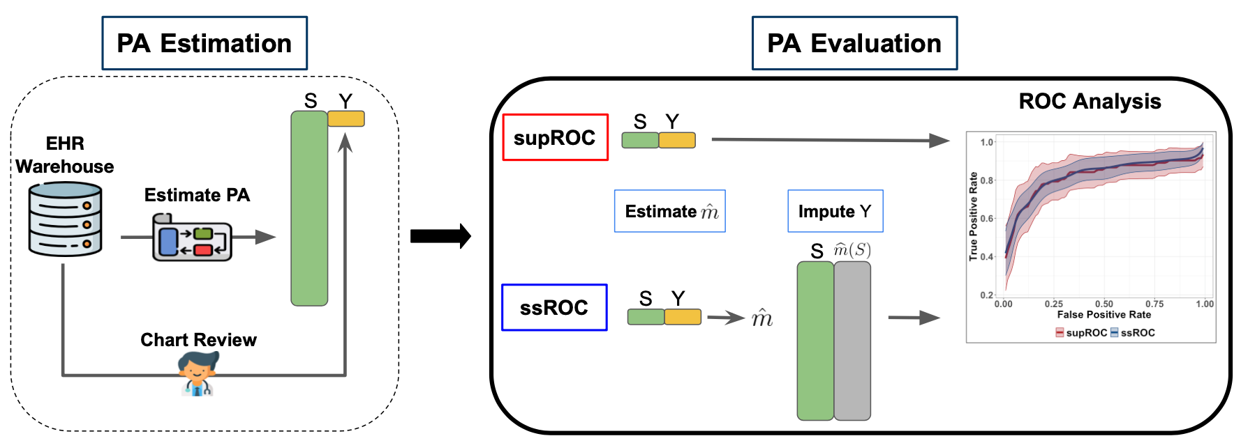
Figure 1: Overview of PA estimation and evaluation. The phenotyping algorithm (PA) is first estimated to obtain the scores ($S$). Patient charts from the electronic health record (EHR) warehouse are reviewed to obtain the gold-standard label ($Y$) for PA evaluation. In classical supervised ROC analysis (supROC), only the labeled data from chart review is used to evaluate the PA’s performance. Semi-supervised ROC analysis (ssROC), uses the labeled data to impute the missing $Y$ as ${\widehat{m}}(S)$ so that the unlabeled data can be utilized for estimation to yield more precise estimates of the ROC parameters.

Data structure & notation

More concretely, the available data in the semi-supervised (SS) setting consists of a small labeled dataset

$$\mathscr{L}=\left\{(Y_{i},S_{i})\mid i=1,\ldots,n\right\}$$

and an unlabeled dataset

$$\mathscr{U}=\left\{S_{i}\mid i=n+1,\ldots,n+N\right\}.$$

In the classical setting, it is assumed that (i) $\mathscr{U}$ is a much larger than $\mathscr{L}$ so that $n\ll N$ and (ii) the observations in $\mathscr{L}$ are randomly selected from the underlying pool of data. Throughout our discussion, we suppose that a higher value of $S$ is more indicative of the phenotype. An observation is deemed to have the phenotype if $S>c$, where $c$ is the threshold for classification.

ROC analysis

More formally, ROC analysis evaluates a PA with the true positive rate (TPR), false positive rate (FPR), positive predictive value (PPV), and negative predictive value (NPV). In diagnostic testing, the TPR is referred to as sensitivity, while the FPR is 1 minus the specificity [45]. For a given classification threshold, one may evaluate the ROC parameters by enumerating the correct and incorrect classifications. This information can be summarized in a confusion matrix as shown in Figure 2.

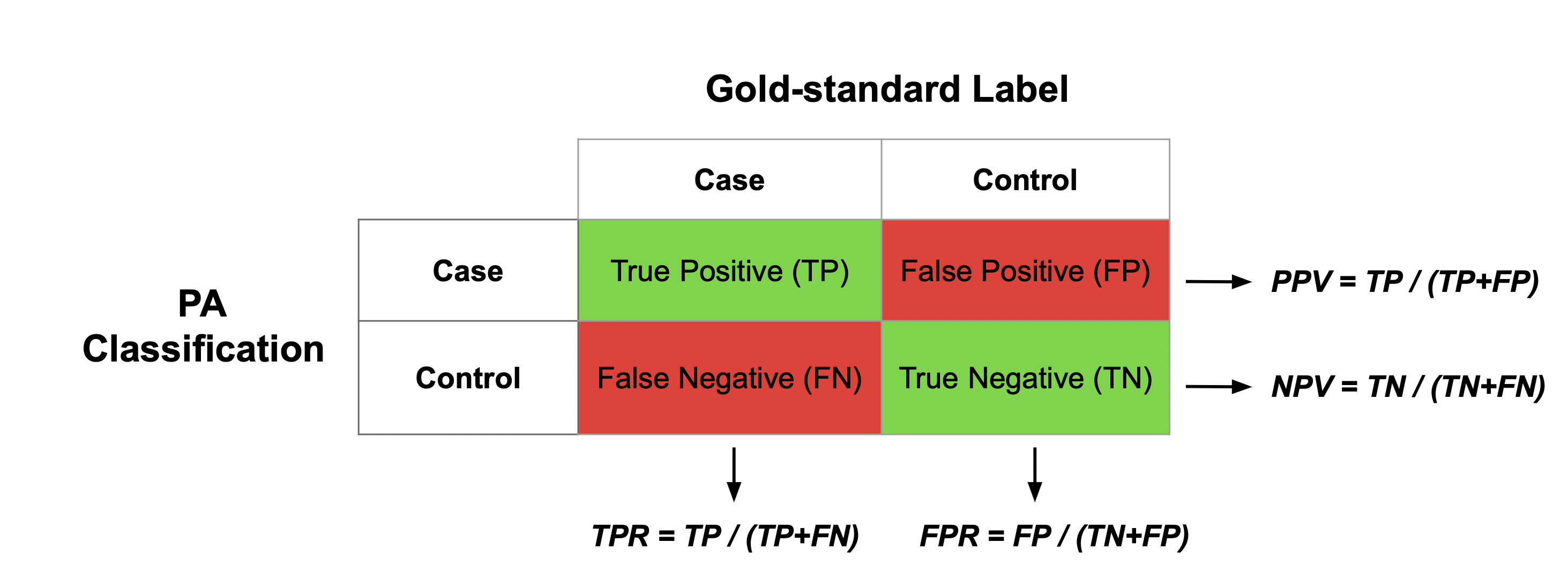
Figure 2: Confusion matrix. The algorithm score from the PA is used to determine phenotype case/control status based on the classification threshold. The ROC parameters are evaluated by enumerating the number of correct and incorrect classifications relative to the gold-standard label.

In practice, it is the task of the researcher to estimate an appropriate threshold for classification. This is commonly done by summarizing the trade-off between the TPR and FPR, defined respectively as

$$\textrm{TPR}(c)=P(S>c\ \mid\ Y=1)\text{ and }\textrm{FPR}(c)=P(S>c\ \mid\ Y=0).$$

The ROC curve, $\textrm{ROC}(u)=\textrm{TPR}[\textrm{FPR}^{-1}(u)]$, summarizes the TPR and FPR across all possible choices of the threshold. In the context of PAs, $c$ is often chosen to achieve a low FPR [22]. An overall summary measure of the discriminative power of $S$ in classifying $Y$ is captured by the area under the ROC curve (AUC),

$$\mbox{AUC}=\int_{0}^{1}\textrm{ROC}(u)du.$$

The AUC is equivalent to the probability that a phenotype case has a higher value of $S$ than a phenotype control. For a given threshold, the predictive performance of the classification rule derived from the PA is assessed with the PPV and NPV, defined respectively as

$$\textrm{PPV}(c)=P(Y=1\ \mid\ S>c), \quad\mbox{and}\quad\textrm{NPV}(c)=P(Y=0\ \mid\ S<c).$$

Supervised ROC analysis

With only labeled data, one may obtain supervised estimators of the ROC parameters (supROC) with their empirical counterparts. For example, the TPR and FPR can be estimated as

$$\widehat{\textrm{TPR}}_{sup}(c)=\frac{\sum_{i=1}^{n}Y_{i}I(S_{i}>c)}{\sum_{i=1}^{n}Y_{i}}\text{ and }\widehat{\textrm{FPR}}_{sup}(c)=\frac{\sum_{i=1}^{n}(1-Y_{i})I(S_{i}>c)}{\sum_{i=1}^{n}(1-Y_{i})}.$$

The remaining parameters are estimated in a similar fashion. Variance estimates can be obtained from a resampling procedure, such as bootstrap or perturbation resampling [46].

ssROC: Semi-supervised ROC Analysis

Unlike its supervised counterpart that relies on only the labeled data, ssROC contains two steps of estimation to make use of the unlabeled data and provide a more reliable understanding of PA performance. In the first step, the missing labels are imputed by recalibrating the PA scores using a model trained with the labeled data. In the second step, the imputations are used in lieu of the gold-standard labels to evaluate the ROC parameters based on the PA scores in the unlabeled data in an analogous manner to supROC. Below we provide an overview of these two steps using the TPR as an example.

Step 1.

Recalibrate the PA scores by fitting the model $m(S)=P(Y=1\mid S)$ with the labeled data. Obtain the imputations, $\{\widehat{m}(S_{i})\mid i=n+1,\dots,n+N\}$, for the unlabeled data using the fitted model.

Step 2.

Use the imputations to estimate the TPR with the unlabeled data as

$$\widetilde{\textrm{TPR}}_{ssROC}(c)=\frac{\sum_{i=n+1}^{n+N}\widehat{m}(S_{i})I(S_{i}>c)}{\sum_{i=n+1}^{n+N}\widehat{m}(S_{i})}.$$

The purpose of the first step is to ensure that the imputations do not introduce bias into the ROC parameter estimates. For example, utilizing the PA scores directly for imputation can distort the ROC parameter estimates due to potential inaccuracies of $S$ in predicting $Y$. We propose to use a kernel regression model to nonparametrically impute the missing labels to prevent biasing the ssROC estimates [40]. Technical detail related to fitting the kernel regression model is provided in Supplementary Section LABEL:supp-ssdetail. In contrast, the purpose of the second step is to harness the large unlabeled dataset to produce estimates with lower variance than supROC. Similar to supROC, we propose a perturbation resampling procedure for variance estimation and detail two commonly used confidence intervals (CIs) based on the procedure in Supplementary Section LABEL:supp-ssinference. In Supplementary Section LABEL:supp-theory, we also provide a theoretical justification for the improved precision of ssROC relative to supROC for a wide range of weakly-supervised PAs.

Data and metrics for evaluation

We assessed the performance of ssROC using simulated, semi-synthetic, and real-world EHR data from MGB. All analyses used the R software package, ssROC, available at https://github.com/jlgrons/ssROC.

Simulation study

Our simulations cover PAs with high and low accuracy and varying degrees of calibration. For each accuracy setting, we simulated PA scores that (i) were perfectly calibrated, (ii) overestimated the probability of $Y$, and (iii) underestimated the probability of $Y$ [47]. In all settings, $Y$ was generated from a Bernoulli distribution with a prevalence of 0.3. To generate $S$, we first generated a random variable $Z$ from a normal mixture model with $Z\mid Y=y\sim N(\alpha_{y},\sigma^{2})$ and an independent noise variable from a Bernoulli mixture model with $\epsilon\mid Y=y\sim\textrm{Bern}(p_{y})$ for $y=0,1$. The PA score was obtained as

$$S=\begin{cases}\text{expit}(\gamma_{0}+\gamma_{1}Z)&\text{for perfect calibration}\\ \text{expit}(Z+\epsilon)&\text{otherwise}\end{cases}$$ (1)

where $\gamma_{0}=(\alpha_{1}^{2}-\alpha_{0}^{2})/2\sigma^{2}+\log\left[(1-\mu)/\mu)\right]$, $\gamma_{1}=(\alpha_{1}-\alpha_{0})/\sigma^{2}$, $\mu=P(Y=1)$, and $\text{expit}(x)=\frac{1}{1+e^{-x}}$. The values of $\gamma_{0}$ and $\gamma_{1}$ ensure that $S=P(Y=1\mid Z)$ for perfect calibration. Six simulation settings were obtained by varying $(\alpha_{0},\alpha_{1},\sigma,p_{0},p_{1})$, shown in Table 1. We also considered the extreme setting when $S$ is independent of $Y$ by permuting $S$ generated from the model with high accuracy and perfect calibration. The calibration curves for each setting are presented in Supplementary Figure LABEL:fig:supp-sim-calibration. Across all settings, $N=10,000$, $n=$ 75, 150, 250 and 500, and results are summarized across 5,000 simulated datasets.

	High PA Accuracy	Low PA Accuracy
Perfectly Calibrated PA	(-0.5, 0.5, 0.5)	(-0.25, 0.25, 0.5)
Overestimated PA	(1, 2.3, 0.5, 0.3, 0.3)	(0.5, 1.2, 0.5, 0.5, 0.5)
Underestimated PA	(-2.6, -1.5, 0.5, 0.1, 0.1)	(-2.5, -1.5, 1, 0.3, 0.3)

Table 1: Parameter configurations for the 6 simulation studies. The simulation settings were derived by varying the parameters $(\alpha_{0},\alpha_{1},\sigma,p_{0},p_{1})$ in Model 1.

Semi-synthetic data analysis

To better reflect the complexity of PAs in real data, we generated semi-synthetic data for phenotyping depression with the MIMIC-III clinical database. MIMIC-III contains structured and unstructured EHR data from patients in the critical care units of the Beth Israel Deaconess Medical Center between 2001 and 2012 [48, 21]. As depression status is unavailable in patient records, it was simulated for all observations using a logistic regression model. That is, $Y\sim\textrm{Bern}[\text{expit}(\bm{\beta}^{T}{\bf X})]$ where

$$\bm{\beta}=(\beta_{0},\beta_{1},\beta_{2},\beta_{3}) {\bf X}=(1,\textrm{log}(X_{NLP}+X_{ICD}+1),X_{age},\textrm{log}(X_{HU}+1))^{T}$$,

$X_{NLP}$ is the number of depression related clinical concepts, $X_{ICD}$ is the number of depression related ICD-9 codes, $X_{age}$ is age at admission, and $X_{HU}$ is a measure of healthcare utilization based on the total number of evaluation and management Current Procedural Terminology (CPT) codes and the length of stay. The list of depression-related ICD-9 codes and clinical concepts are presented in Supplementary Section LABEL:supp-semisyn.

Given the PA score is obtained from complex EHR data, we focus on simulating the phenotype to achieve high and low PA accuracy and present the calibration in Supplementary Figure LABEL:fig:semi-syn-calirabtion. We set $\bm{\beta}=(1,4,0.05,-3)$ and $\bm{\beta}=(1,1,0.01,-1)$ and to mimic a PA with high and low accuracy (AUC = 90.1 and 72.6, respectively). The prevalence of $Y$ in both settings was approximately 0.3. For both settings, the unlabeled set consisted of one visit from $N=32,172$ unique patients and $n=$ 75, 150, 250, and 500 visits were randomly sampled 5,000 times to generate labeled datasets of various sizes. We obtained the PA for depression by fitting PheNorm without the random corruption denoising step. PheNorm is a weakly-supervised method based on normalizing silver-standard labels with respect to patient healthcare utilization using a normal mixture model [43]. PheNorm is also used in our real-data analysis and described in detail in Supplementary Section LABEL:supp-phenorm. $X_{NLP}$ and $X_{ICD}$ were used as silver-standard labels to fit PheNorm with $X_{HU}$ as the measure of healthcare utilization.

Real-world EHR data application

We further validated ssROC using EHR data from MGB, a Boston-based healthcare system anchored by two tertiary care centers, Brigham and Women’s Hospital and Massachusetts General Hospital. We evaluated PAs for five phenotypes, including Cerebral Aneurysm (CA), Congestive Heart Failure (CHF), Parkinson’s Disease (PD), Systemic Sclerosis (SS), and Type 1 Diabetes (T1DM). The data is from the Research Patient Data Registry which stores data on over 1 billion visits containing diagnoses, medications, procedures, laboratory information, and clinical notes from 1991 to 2017.

The full data for each phenotype consisted of patient records with at least one phenotype-related PheCode in their record [49]. A subset of patients was randomly sampled from the full data and sent for chart review. For each phenotype, the PA was obtained by fitting PheNorm without denoising using the total number of (i) phenotype-related PheCodes and (ii) positive mentions of the phenotype-related clinical concepts as the silver standard labels and the number of notes in a patient’s EHR as the measure of healthcare utilization. The phenotypes represent different levels of PA accuracy, labeled and unlabeled dataset sizes, and prevalence ($P$). A summary of the five phenotypes is presented in Table  2.

Phenotype	$n$	$N$	$P$	PheCode	CUI
Cerebral Aneurysm (CA)	134	18,679	0.68	433.5	C0917996
Congestive Heart Failure (CHF)	140	155,112	0.18	428	C0018801
Parkinson’s Disease (PD)	97	17,752	0.62	332	C0030567
Systemic Sclerosis (SS)	189	4,272	0.43	709.3	C0036421
Type 1 Diabetes (T1DM)	121	46,013	0.17	250.1	C0011854

Table 2: Summary of the MGB Phenotypes. The labeled dataset size ($n)$, the unlabeled dataset size ($N$), and the prevalence ($P$) of the five phenotypes as well as the main PheCode and concept unique identifier (CUI) used to train PheNorm. The underlying full data for each phenotype included all participants who passed the filter of $\geq 1$ PheCode for the phenotype of interest.

Benchmark method and reported metrics

We compared the PA evaluation results from ssROC and the benchmark, supROC, using the simulated, semi-synthetic, and real EHR data. We transformed the PA scores by their respective empirical cumulative distribution functions prior to ROC analysis. This transformation improves the performance of the imputation step, particularly when the distribution of $S$ is skewed [50]. For the kernel regression, we used a Gaussian kernel with bandwidth determined by the standard deviation of the transformed PA scores divided by $n^{0.45}$ [51]. Additional detail related to the imputation step is provided in Supplementary Section LABEL:supp-ssdetail. We obtained variance estimates for the ROC parameters using perturbation resampling with 500 replications and weights from a scaled beta distribution, $4\cdot\text{Beta}(1/2,3/2)$, to improve finite-sample performance [52]. We focused on logit-based confidence intervals (CIs), described in Supplementary Section LABEL:supp-ci, due to their improved coverage relative to standard Wald intervals [53].

We assessed percent bias for both supROC and ssROC by computing the mean of [(point estimate - ground truth)/ (ground truth) * 100%] across the replicated datasets. The ground truth values of the ROC parameters for the simulated and semi-synthetic data are provided in Supplementary Tables LABEL:tab:supp-oracle-sim and LABEL:tab:supp-oracle-semi. The empirical standard error (ESE) was computed as the standard deviation of the estimates from these datasets. The asymptotic standard error (ASE) was computed as the mean of the standard error estimates derived from the perturbation resampling procedure across the replicated datasets. Using mean squared error (MSE) as an aggregate measure of bias and variance, we evaluated the relative efficiency (RE) as the ratio of the MSE of supROC to the MSE of ssROC. The performance of our resampling procedure was assessed with the coverage probability (CP) of the 95% CIs for both estimation procedures. In the real data analysis, we present point estimates from both supROC and ssROC and the RE defined as the ratio of the variance of supROC to ssROC. We evaluated the performance of the PAs at an FPR of 10% and report the results for the AUC, classification threshold (Threshold), TPR, PPV, and NPV for all analyses.

RESULTS

Simulation study

Figures 3 and 4 show the percent bias and RE in the high and low accuracy settings, respectively. Both ssROC and supROC generally exhibit low bias across all settings and ssROC often has lower bias than supROC. Additionally, ssROC has lower variance than supROC in all settings, as indicated by REs that consistently exceed 1. In the high accuracy setting, the median REs across all calibration patterns and labeled sizes, is between 1.3 (AUC) and 1.9 (Threshold). For the low accuracy setting, the median REs range from 1.1 (AUC) to 1.6 (Threshold). Practically, these results imply that ssROC is more precise for a fixed amount of labeled than supROC. Alternatively, this reduction in variance can also be interpreted as a reduction in sample size required for ssROC to achieve the same variance as supROC. For example, the RE for PPV with $n=250$ under the setting of high PA accuracy and calibrated PA is 2, which suggests that ssROC can achieve the same variance as supROC with half the amount of labeled data.

When $S$ is independent of $Y$, Supplementary Figure LABEL:fig:sim_pbias_indep shows that ssROC has negligible bias, yields precision similar to supROC for the ROC parameters, and has improved precison for the threshold. These empirical findings demonstrate the robustness of ssROC to a wide range of PA scores and are further supported by our theoretical analysis in Supplementary Section LABEL:supp-theory. Specifically, our analysis verifies that ssROC is guaranteed to perform on par supROC for the ROC parameters and yield more precise estimation for the threshold when $S$ is independent of $Y$.

The ESE, ASE, and CP for the 95% confidence intervals (CIs) of both supROC and ssROC are presented in Supplementary Tables LABEL:tab:supcp and LABEL:tab:sscp. The proposed logit-based CI consistently achieve reasonable coverage for both methods. The estimated variance for ssROC is also generally more accurate than that from supROC. Additionally, our results underscore the advantages of employing the logit-based interval over the standard Wald interval, particularly when $n$ is small and/or the point estimate is near the boundary.

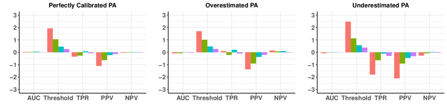
(a) Percent Bias of supROC

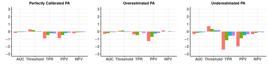
(b) Percent Bias of ssROC

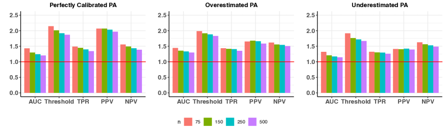
(c) Relative Efficiency (supROC : ssROC)

Figure 3: Percent bias and relative efficiency (RE) for high PA accuracy settings at a FPR of 10%. RE is defined as the mean squared error of supROC compared to the mean squared error of ssROC. For all scenarios, the size of the unlabeled was $N=10,000$.

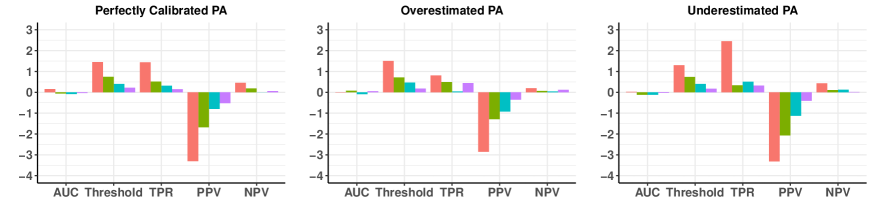
(a) Percent Bias of supROC

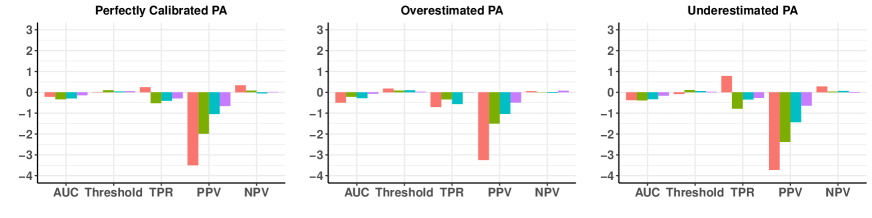
(b) Percent Bias of ssROC

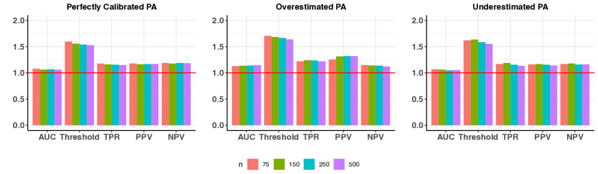
(c) Relative Efficiency (supROC : ssROC)

Figure 4: Percent bias and relative efficiency (RE) for low PA accuracy settings at a FPR of 10%. RE is defined as the mean squared error of supROC compared to the mean squared error of ssROC. For all scenarios, the size of the unlabeled was $N=10,000$.

Semi-synthetic data analysis

The findings from the semi-synthetic EHR data analysis align closely with the results of our simulations, further demonstrating the robustness of ssROC to the PA score. Generally, ssROC has smaller bias than supROC and both methods have small bias across all settings as highlighted in Figure  5 (a) and (b). ssROC again demonstrates improved precision relative to supROC. The median RE across labeled data sizes in settings with high PA accuracy is between 1.3 (AUC) and 1.9( Threshold) and between 1.1 (AUC) and 2.1 (Threshold) for the low accuracy setting. Additionally, Supplementary Tables LABEL:tab:semi-sup-cp and LABEL:tab:semi-ss-cp show that the logit-based CIs for both methods yield reasonable coverage.

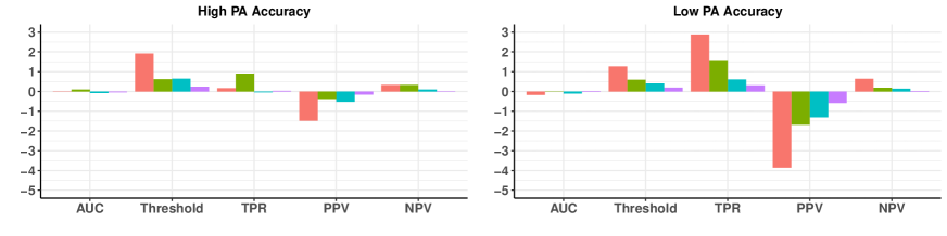
(a) Percent Bias of supROC

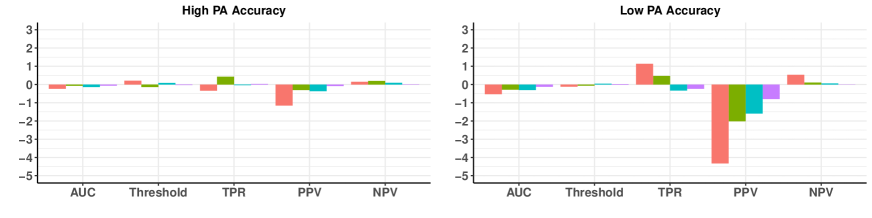
(b) Percent Bias of ssROC

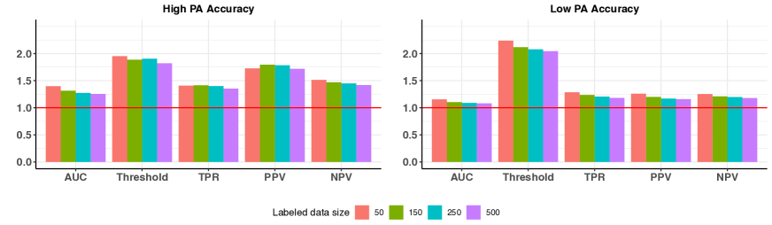
(c) Relative Efficiency (supROC : ssROC)

Figure 5: Percent bias and relative efficiency (RE) for the semi-synthetic data analysis at a FPR of 10%. RE is defined as the mean squared error of supROC compared to the mean squared error of ssROC. For both settings, the size of total data was 32,172.

Analysis of five PAs from MGB

Table 3 presents the point estimates for the five phenotypes from MGB, ordered by the AUC estimates from ssROC, at a false positive rate (FPR) of 10%. As our primary focus is to compare ssROC with supROC, a single FPR was chosen for consistency across the phenotypes. However, this does lead to low TPRs for some phenotypes, such as CHF. Generally, the point estimates from ssROC are similar to those from supROC. There are some differences in the classification threshold estimates for CA and SS, which leads to some discrepancies in the other estimates. As supROC is only evaluated at the unique PA scores in the labeled dataset, the threshold estimate can be unstable at some FPRs. In contrast, ssROC is evaluated across a broader range of PA scores in the unlabeled dataset and results in a more stable estimation.

Phenotype	Method	AUC	Threshold	TPR	PPV	NPV
CA	ssROC	81.3	64.0	51.0	89.8	51.5
	supROC	80.4	73.7	35.2	87.4	40.1
CHF	ssROC	83.2	84.9	42.0	44.1	89.2
	supROC	79.3	86.1	36.0	43.9	86.6
PD	ssROC	85.9	75.3	49.1	74.1	75.2
	supROC	81.6	80.1	34.1	72.4	64.1
SS	ssROC	89.4	59.8	60.6	89.9	60.7
	supROC	87.5	64.6	52.3	89.7	53.2
T1DM	ssROC	90.5	80.4	68.8	57.3	93.7
	supROC	91.5	80.1	75.0	59.8	94.8

Table 3: Point estimates for the 5 phenotypes from MGB at a FPR of 10%.

Figure 6 shows the RE of supROC to ssROC across the five phenotypes at a FPR of 10%. The median RE gain across phenotypes ranges from approximately 1.5 (AUC, TPR) to 2.7 (Threshold), implying that the estimates from ssROC are approximately 30% – 60% less variable than supROC on average. It is worth noting the RE for the threshold estimate for CHF is quite high. Supplementary Figure LABEL:fig:supp-cut_pert illustrates that this behavior can be explained by the empirical distribution of the resampled estimates. The distribution of the estimates from supROC are multimodal, while those from ssROC are approximately normal as expected. This behavior further emphasizes the stability of ssROC relative to supROC in real data.

Consistent with our simulation and theoretical results, we also observe that RE is linked to PA accuracy. For example, a phenotype with high PA accuracy, such as T1DM, exhibits a higher RE compared to CA, which has the lowest PA accuracy. Overall, these findings underscore the advantages of our proposed ssROC method compared to supROC in yielding more precise ROC analysis.

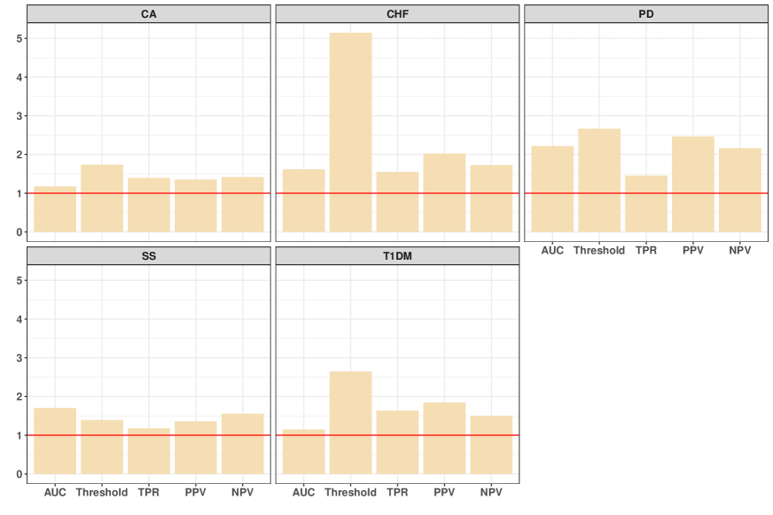
Figure 6: Relative efficiency (RE) for the 5 phenotypes from MGB at an FPR of 10%. RE is defined as the ratio of the variance of supROC to that of ssROC.

DISCUSSION

Although high-throughput phenotyping is the backbone of EHR-based research, there is a paucity of methods for reliably evaluating the predictive performance of a PA with limited labeled data. The proposed ssROC method fills this gap. ssROC is a simple two-step estimation procedure that leverages large volumes of unlabeled data by imputing missing gold-standard labels with a nonparametric recalibration of a PA score. Unlike existing procedures for PA evaluation in the informatics literature, ssROC eliminates the requirement that the PA be correctly specified to yield unbiased estimation of the ROC parameters and may be utilized for ML-based PAs [25, 37]. While we focus specifically on weakly-supervised PAs in our theoretical analysis and data examples given their increasing popularity and ability to automate PA estimation, ssROC can also be used to evaluate rule-based or other ML-based PAs. Moreover, by harnessing unlabeled data, ssROC yields substantially less variable estimates than supROC in simulated, semi-synthetic, and real data. Practically, this translates into a significant reduction in the amount of chart review required to obtain a precise understanding of PA performance.

Although our work is a first step toward streamlining PA evaluation, there are several avenues that warrant future research. First, ssROC assumes that the labeled examples are randomly sampled from the underlying full data. In situations where the goal is to phenotype multiple conditions or comorbidities, more effective sampling strategies such as stratified random sampling have the potential to further enhance the efficiency of ssROC [54]. However, due to the large discrepancy in size of the labeled and unlabeled data, developing procedures to accommodate non-random sampling is nontrivial [55]. Second, the nonparametric recalibration step demands a sufficient amount of labeled data for the kernel regression to be well estimated. While our extensive simulation studies across a wide variey of PAs and sample sizes illustrate the robustness of ssROC, our future work will develop a parametric recalibration procedure that accommodates smaller labeled data sizes. Third, ssROC can also be extended for model comparisons and evaluation of fairness metrics, which are urgently needed given the increasing recognition of unfairness in informatics applications. The calibration step would need to be augmented in both settings to utilize additional information in multiple PA scores or protected attributes, respectively. This augmentation could potentially lead to a more efficient procedure as ssROC only uses information from one PA score for imputation. Lastly, our results demonstrate the ability of ssROC to provide accurate ROC evaluation for five phenotypes with variable prevalence, labeled and unlabeled dataset sizes, and PA accuracy within one health system. Further work is needed to understand the performance of our method across a diverse range of phenotypes and to extend our approach to accommodate federated analyses across multiple healthcare systems.

CONCLUSION

In this paper, we introduced a semi-supervised approach, ssROC, that leverages a large volume of unlabeled data together with a small subset of gold-standard labeled data to precisely estimate the ROC parameters of PAs. PA development involves two key steps: (i) algorithm estimation and (ii) algorithm evaluation. While a considerable amount of effort has been placed on algorithm estimation, ssROC fills the current gap in robust and efficient methodology for predictive performance evaluation. Additionally, ssROC is simple to implement and is available in open-source R software to encourage use in practice. When used in conjunction with weakly-supervised PAs, ssROC demonstrates the potential to facilitate the reliable and streamlined phenotyping that is necessary for a wide variety of translational EHR applications.

FUNDING

The project was supported by the Natural Sciences and Engineering Research Council of Canada grant (RGPIN-2021-03734), the University of Toronto Connaught New Researcher Award, and the University of Toronto Seed Funding for Methodologists Grant (to JeG).

AUTHOR CONTRIBUTIONS

JeG conceived and designed the study. JiG conducted simulation and semi-synthetic data analyses. CB and CH conducted real data analyses. JeG, JiG, CB, PV, and KZ analyzed and interpreted the results. JeG and JiG drafted and revised the manuscript. All authors reviewed and approved the final manuscript.

CONFLICT OF INTEREST STATEMENT

The authors have no conflicts of interest to declare.

DATA AND CODE AVAILABILITY

Our proposed method is implemented as an R software package, ssROC, which is available at https://github.com/jlgrons/ssROC.

References

- [1] J Michael McGinnis et al. “Clinical data as the basic staple of health learning: Creating and protecting a public good: Workshop summary” National Academies Press, 2011
- [2] Kenneth S Boockvar et al. “Electronic health records and adverse drug events after patient transfer” In Quality and Safety in Health Care 19.5 BMJ Publishing Group Ltd, 2010, pp. e16–e16
- [3] Fina Kurreeman et al. “Genetic basis of autoantibody positive and negative rheumatoid arthritis risk in a multi-ethnic cohort derived from electronic health records” In The American Journal of Human Genetics 88.1 Elsevier, 2011, pp. 57–69
- [4] Katherine P Liao et al. “Associations of autoantibodies, autoimmune risk alleles, and clinical diagnoses from the electronic medical records in rheumatoid arthritis cases and non–rheumatoid arthritis controls” In Arthritis & Rheumatism 65.3 Wiley Online Library, 2013, pp. 571–581
- [5] Chia-Yen Chen et al. “Genetic validation of bipolar disorder identified by automated phenotyping using electronic health records” In Translational psychiatry 8.1 Nature Publishing Group, 2018, pp. 1–8
- [6] Ruowang Li et al. “Electronic health records and polygenic risk scores for predicting disease risk” In Nature Reviews Genetics Nature Publishing Group, 2020, pp. 1–10
- [7] Gabriel A Brat et al. “International electronic health record-derived COVID-19 clinical course profiles: the 4CE consortium” In NPJ digital medicine 3.1 Nature Publishing Group, 2020, pp. 1–9
- [8] Lisa Bastarache “Using phecodes for research with the electronic health record: from PheWAS to PheRS” In Annual review of biomedical data science 4 Annual Reviews, 2021, pp. 1–19
- [9] Daniel Prieto-Alhambra et al. “Unraveling COVID-19: a large-scale characterization of 4.5 million COVID-19 cases using CHARYBDIS” In Research square American Journal Experts, 2021
- [10] Katharine E Henry et al. “Factors driving provider adoption of the TREWS machine learning-based early warning system and its effects on sepsis treatment timing” In Nature medicine 28.7 Nature Publishing Group US New York, 2022, pp. 1447–1454
- [11] Chaitanya Shivade et al. “A review of approaches to identifying patient phenotype cohorts using electronic health records” In Journal of the American Medical Informatics Association 21.2 BMJ Publishing Group, 2014, pp. 221–230
- [12] Juan M Banda et al. “Advances in electronic phenotyping: from rule-based definitions to machine learning models” In Annual review of biomedical data science 1 NIH Public Access, 2018, pp. 53
- [13] Hadeel Alzoubi et al. “A review of automatic phenotyping approaches using electronic health records” In Electronics 8.11 MDPI, 2019, pp. 1235
- [14] Siyue Yang et al. “Machine learning approaches for electronic health records phenotyping: a methodical review” In Journal of the American Medical Informatics Association 30.2 Oxford University Press, 2023, pp. 367–381
- [15] Yichi Zhang et al. “High-throughput phenotyping with electronic medical record data using a common semi-supervised approach (PheCAP)” In Nature Protocols 14.12 Nature Publishing Group, 2019, pp. 3426–3444
- [16] Shawn Murphy et al. “Instrumenting the health care enterprise for discovery research in the genomic era” In Genome research 19.9 Cold Spring Harbor Lab, 2009, pp. 1675–1681
- [17] Victor Castro et al. “Identification of subjects with polycystic ovary syndrome using electronic health records” In Reproductive Biology and Endocrinology 13.1 Springer, 2015, pp. 116
- [18] Pedro L Teixeira et al. “Evaluating electronic health record data sources and algorithmic approaches to identify hypertensive individuals” In Journal of the American Medical Informatics Association 24.1, 2017, pp. 162–171
- [19] Alon Geva et al. “A computable phenotype improves cohort ascertainment in a pediatric pulmonary hypertension registry” In The Journal of pediatrics 188 Elsevier, 2017, pp. 224–231
- [20] Christopher Meaney et al. “Using Biomedical Text as Data and Representation Learning for Identifying Patients with an Osteoarthritis Phenotype in the Electronic Medical Record” In International Journal of Population Data Science 3.4, 2018
- [21] Sebastian Gehrmann et al. “Comparing deep learning and concept extraction based methods for patient phenotyping from clinical narratives” Publisher: Public Library of Science In PLOS ONE 13.2, 2018, pp. e0192360 DOI: 10.1371/journal.pone.0192360
- [22] Katherine P Liao et al. “High-throughput multimodal automated phenotyping (MAP) with application to PheWAS” In Journal of the American Medical Informatics Association 26.11 Oxford University Press, 2019, pp. 1255–1262
- [23] Vijay S. Nori et al. “Deep neural network models for identifying incident dementia using claims and EHR datasets” In PLOS ONE 15, 2020, pp. e0236400
- [24] Yizhao Ni et al. “Automated detection of substance use information from electronic health records for a pediatric population” In Journal of the American Medical Informatics Association 28, 2021, pp. 2116–2127
- [25] Joel N Swerdel, George Hripcsak and Patrick B Ryan “PheValuator: development and evaluation of a phenotype algorithm evaluator” In Journal of biomedical informatics 97 Elsevier, 2019, pp. 103258
- [26] Christian Chartier, Lisa Gfrerer and William G. Austen “ChartSweep: A HIPAA-compliant Tool to Automate Chart Review for Plastic Surgery Research” In Plastic and Reconstructive Surgery - Global Open 9, 2021, pp. e3633
- [27] Sheng Yu et al. “Toward high-throughput phenotyping: unbiased automated feature extraction and selection from knowledge sources” In Journal of the American Medical Informatics Association 22.5 The Oxford University Press, 2015, pp. 993–1000
- [28] Sheng Yu et al. “Surrogate-assisted feature extraction for high-throughput phenotyping” In Journal of the American Medical Informatics Association 24.e1 Oxford University Press, 2017, pp. e143–e149
- [29] Isabelle-Emmanuella Nogues et al. “Weakly Semi-supervised phenotyping using Electronic Health records” In Journal of Biomedical Informatics 134 Elsevier, 2022, pp. 104175
- [30] Adam Wright, Elizabeth S Chen and Francine L Maloney “An automated technique for identifying associations between medications, laboratory results and problems” In Journal of biomedical informatics 43.6 Elsevier, 2010, pp. 891–901
- [31] Adam Wright et al. “A method and knowledge base for automated inference of patient problems from structured data in an electronic medical record” In Journal of the American Medical Informatics Association 18.6 BMJ Group BMA House, Tavistock Square, London, WC1H 9JR, 2011, pp. 859–867
- [32] Vibhu Agarwal et al. “Learning statistical models of phenotypes using noisy labeled training data” In Journal of the American Medical Informatics Association 23.6 Oxford University Press, 2016, pp. 1166–1173
- [33] Juan M Banda et al. “Electronic phenotyping with APHRODITE and the Observational Health Sciences and Informatics (OHDSI) data network” In AMIA Summits on Translational Science Proceedings 2017 American Medical Informatics Association, 2017, pp. 48
- [34] Jing Huang et al. “PIE: A prior knowledge guided integrated likelihood estimation method for bias reduction in association studies using electronic health records data” In Journal of the American Medical Informatics Association 25.3 Oxford University Press, 2018, pp. 345–352
- [35] Jiayi Tong et al. “An augmented estimation procedure for EHR-based association studies accounting for differential misclassification” In Journal of the American Medical Informatics Association 27.2 Oxford University Press, 2020, pp. 244–253
- [36] Ziyan Yin et al. “A cost-effective chart review sampling design to account for phenotyping error in electronic health records (EHR) data” In Journal of the American Medical Informatics Association 29.1 Oxford University Press, 2022, pp. 52–61
- [37] Joel N Swerdel et al. “PheValuator 2.0: Methodological improvements for the PheValuator approach to semi-automated phenotype algorithm evaluation” In Journal of Biomedical Informatics 135 Elsevier, 2022, pp. 104177
- [38] Jessica L Gronsbell and Tianxi Cai “Semi-supervised approaches to efficient evaluation of model prediction performance” In Journal of the Royal Statistical Society: Series B (Statistical Methodology) 80.3 Wiley Online Library, 2018, pp. 579–594
- [39] Jessica Gronsbell et al. “Efficient estimation and evaluation of prediction rules in semi-supervised settings under stratified sampling” In arXiv preprint arXiv:2010.09443, 2020
- [40] Ben Van Calster et al. “Calibration: the Achilles heel of predictive analytics” In BMC medicine 17.1 Springer, 2019, pp. 1–7
- [41] Yingxiang Huang et al. “A tutorial on calibration measurements and calibration models for clinical prediction models” In Journal of the American Medical Informatics Association 27.4 Oxford University Press, 2020, pp. 621–633
- [42] Juan M. Banda et al. “Electronic phenotyping with APHRODITE and the Observational Health Sciences and Informatics (OHDSI) data network” In AMIA Summits on Translational Science Proceedings 2017, 2017, pp. 48–57
- [43] Sheng Yu et al. “Enabling phenotypic big data with PheNorm” In Journal of the American Medical Informatics Association 25.1 Oxford University Press, 2018, pp. 54–60
- [44] Jessica Gronsbell et al. “Automated feature selection of predictors in electronic medical records data” In Biometrics 75.1 Wiley Online Library, 2019, pp. 268–277
- [45] Margaret Sullivan Pepe “The statistical evaluation of medical tests for classification and prediction” Oxford University Press, 2003
- [46] Jessica Minnier, Lu Tian and Tianxi Cai “A Perturbation Method for Inference on Regularized Regression Estimates” In Journal of the American Statistical Association 106.496 TaylorFrancis Ltd, 2011, pp. 1371–1382
- [47] Ben Van Calster et al. “Calibration: The Achilles Heel of Predictive Analytics” In BMC Medicine 17.1, 2019, pp. 230
- [48] Alistair E.. Johnson et al. “MIMIC-III, a freely accessible critical care database” Number: 1 Publisher: Nature Publishing Group In Scientific Data 3.1, 2016, pp. 160035
- [49] Joshua C Denny et al. “Systematic comparison of phenome-wide association study of electronic medical record data and genome-wide association study data” In Nature biotechnology 31.12 Nature Publishing Group, 2013, pp. 1102–1111
- [50] Matthew P Wand, James Stephen Marron and David Ruppert “Transformations in density estimation” In Journal of the American Statistical Association 86.414 Taylor & Francis, 1991, pp. 343–353
- [51] Bernard W Silverman “Density estimation for statistics and data analysis” Routledge, 2018
- [52] Jennifer A Sinnott and Tianxi Cai “Inference for survival prediction under the regularized Cox model” In Biostatistics 17.4 Oxford University Press, 2016, pp. 692–707
- [53] Alan Agresti “Categorical data analysis” John Wiley & Sons, 2012
- [54] W Katherine Tan and Patrick J Heagerty “Surrogate-guided sampling designs for classification of rare outcomes from electronic medical records data” In Biostatistics 23.2 Oxford University Press, 2022, pp. 345–361
- [55] Yuqian Zhang, Abhishek Chakrabortty and Jelena Bradic “Double Robust Semi-Supervised Inference for the Mean: Selection Bias under MAR Labeling with Decaying Overlap” arXiv, 2023 arXiv:2104.06667 [math, stat]