Timescales of Chaos in the Inner Solar System:
Lyapunov Spectrum and Quasi-integrals of Motion

Abstract

Numerical integrations of the Solar System reveal a remarkable stability of the orbits of the inner planets over billions of years, in spite of their chaotic variations characterized by a Lyapunov time of only 5 million years and the lack of integrals of motion able to constrain their dynamics. To open a window on such long-term behavior, we compute the entire Lyapunov spectrum of a forced secular model of the inner planets. We uncover a hierarchy of characteristic exponents that spans two orders of magnitude, manifesting a slow-fast dynamics with a broad separation of timescales. A systematic analysis of the Fourier harmonics of the Hamiltonian, based on computer algebra, reveals three symmetries that characterize the strongest resonances responsible for the orbital chaos. These symmetries are broken only by weak resonances, leading to the existence of quasi-integrals of motion that are shown to relate to the smallest Lyapunov exponents. A principal component analysis of the orbital solutions independently confirms that the quasi-integrals are among the slowest degrees of freedom of the dynamics. Strong evidence emerges that they effectively constrain the chaotic diffusion of the orbits, playing a crucial role in the statistical stability over the Solar System lifetime.

I Introduction

The planetary orbits in the inner Solar System (ISS) are chaotic, with a Lyapunov time distributed around 5 million years (Myr) [1, 2, 3, 4]. Still, they are statistically very stable over a timescale that is a thousand times longer. The probability that the eccentricity of Mercury exceeds 0.7, leading to catastrophic events (i.e., close encounters, collisions, or ejections of planets), is only about 1% over the next 5 billion years (Gyr) [5, 6, 7]. The dynamical half-life of Mercury orbit has recently been estimated at 30–40 billion years [4, 7]. A disparity of nearly four orders of magnitude between the Lyapunov time and the timescale of dynamical instability is intriguing, since the chaotic variations of the orbits of the inner planets cannot be constrained a priori. While the total energy and angular momentum of the Solar System are conserved, the disproportion of masses between the outer and inner planets implies that unstable states of the ISS are in principle easily realizable through exchanges of these quantities. The surprising stability of the ISS deserves a global picture in which it can emerge more naturally.

To our knowledge, the only study addressing the timescale separation in the long-term dynamics of the ISS is based on the simplified secular dynamics of a massless Mercury [8]: All the other planets are frozen on regular quasi-periodic orbits; secular interactions are expanded to first order in masses and degree 4 in eccentricities and inclinations; an a priori choice of the relevant terms of the Hamiltonian is made. The typical instability time of about 1 Gyr [8, 9] is, however, too short and in significant contrast with realistic numerical integrations of the Solar System, which show a general increase of the instability rate with the complexity of the dynamical model [7]. We have shown that truncating the secular Hamiltonian of the ISS at degree 4 in eccentricities and inclinations results in an even more stable dynamics, with an instability rate at 5 Gyr that drops by orders of magnitude when compared to the full system. From the perspective of these latest findings, the small probability of 1% of an instability over the age of the Solar System may be naturally regarded as a perturbative effect of terms of degree 6 and higher. Clearly, the striking stability of the dynamics at degree 4 is even more impressive in the present context, and remains to be explained.

A strong separation in dynamical timescales is not uncommon among classical quasi-integrable systems [e.g., 11, 12]. This is notably evinced by the Fermi-Pasta-Ulam-Tsingou (FPUT) problem, which deals with a chain of coupled weakly-anharmonic oscillators [13]. Far from Kolmogorov-Arnold-Moser (KAM) and Nekhoroshev regimes (as is likely to be pertinent to the ISS, see Sect. III), one can generally state that the exponential divergence of close trajectories occurring over a Lyapunov time is mostly tangent to the invariant tori defined by the action variables of the underlying integrable problem, and hence contributes little to the diffusion in the action space [14, 15]. In other words, the Lyapunov time and the diffusion/instability time scale differently with the size of the terms that break integrability, and this can result in very different timescales [12]. However, this argument is as general as poorly satisfactory in addressing quantitatively the timescale separation in a complex problem as the present one. Moreover, even though order-of-magnitude estimates of the chaotic diffusion in the ISS suggest that it may take hundreds of million years to reach the destabilizing secular resonance $g_{1}-g_{5}$, the low probability of an instability over 5 Gyr still remains unexplained [4]. Establishing more precisely why the ISS is statistically stable over a timescale comparable to its age is a valuable step in understanding the secular evolution of planetary systems through metastable states [17, 4]. With its 8 secular degrees of freedom (d.o.f.), this system also constitutes a peculiar bridge between the low-dimensional dynamics often addressed in celestial mechanics and the systems with a large number of bodies studied in statistical mechanics: It cannot benefit from the straightforward application of standard methods of the two fields [e.g., 19, Appendix A].

This work aims to open a window on the long-term statistical behavior of the inner planet orbits. Section II briefly recalls the dynamical model of forced secular ISS introduced in Ref. [4]. Section III presents the numerical computation of its Lyapunov spectrum. Section IV introduces the quasi-symmetries of the resonant harmonics of the Hamiltonian and the corresponding quasi-integrals (QIs) of motion. Section V establishes a geometric connection between the quasi-integrals and the slowest d.o.f. of the dynamics via a principal component analysis (PCA) of the orbital solutions. Section VI states the implications of the new findings on the long-term stability of the ISS. We finally discuss the connections with other classical quasi-integrable systems and the methods used in this work.

Table 1: Summary of the different models of forced secular ISS considered in this work. Gauss’s dynamics results from first-order averaging of the $N$-body Hamiltonian over the mean longitudes of the planets. The dynamics generated by $\mathcal{H}_{2n}$ and $\mathbb{H}_{2n}$ are practically equivalent and treated as such. The $\mathbb{H}_{2n}^{\bullet}$ models are introduced and discussed in Sec. IV.4.

Hamiltonian	Description	Reference
$\mathcal{H}$	Gauss’s dynamics in complex Poincaré variables	Eq. (4)
$\mathcal{H}_{2n}$	Truncation of Gauss’s dynamics at total degree $2n$ in eccentricities and inclinations	Ref. [4]
$\mathbb{H}_{2n}$	Truncated dynamics in the action-angle variables of the Laplace-Lagrange dynamics $\mathcal{H}_{2}$	Eq. (6) and Ref. [4]
$\mathbb{H}_{2n}^{\bullet}$	Fourier harmonics that involve outer planet modes other than $g_{5}$ are dropped from $\mathbb{H}_{2n}$	Eq. (24)

II Dynamical model

The long-term dynamics of the Solar System planets consists essentially of the slow precession of their perihelia and nodes, driven by secular, orbit-averaged gravitational interactions [2, 20]. At first order in planetary masses, the secular Hamiltonian corrected for the leading contribution of general relativity reads [e.g. 21, 4]

$$\widehat{H}=-\sum_{i=1}^{8}\left[\sum_{l=1}^{i-1}\left<\frac{Gm_{i}m_{l}}{\|\bm{r}_{i}-\bm{r}_{l}\|}\right>+\frac{3G^{2}m_{0}^{2}m_{i}}{c^{2}a_{i}^{2}\sqrt{1-e_{i}^{2}}}\right].$$ (1)

The planets are indexed in order of increasing semi-major axes $(a_{i})_{i=1}^{8}$, $m_{0}$ and $m_{i}$ are the Sun and planet masses, respectively, $e_{i}$ the eccentricities, $G$ the gravitational constant and $c$ the speed of light. The vectors $\bm{r}_{i}$ are the heliocentric positions of the planets, and the bracket operator represents the averaging over the mean longitudes resulting from the elimination of the non-resonant Fourier harmonics of the $N$-body Hamiltonian [21, 4]. Hamiltonian (1) generates Gauss’s dynamics of Keplerian rings [22, 4], whose semi-major axes $a_{i}$ are constants of motion of the secular dynamics.

By developing the 2-body perturbing function [23, 24] in the computer algebra system TRIP [25, 26], the secular Hamiltonian can be systematically expanded in series of the Poincaré rectangular coordinates in complex form,

$$x_{i} =\sqrt{\Lambda_{i}}\sqrt{1-\sqrt{1-e_{i}^{2}}}\mathrm{E}^{j\varpi_{i}},$$ (2)

$$y_{i} =\sqrt{2\Lambda_{i}}\left(1-e_{i}^{2}\right)^{\frac{1}{4}}\sin(\mathcal{I}_{i}/2)\mathrm{E}^{j\Omega_{i}},$$

where $\Lambda_{i}=\mu_{i}[G(m_{0}+m_{i})a_{i}]^{1/2}$, $\mu_{i}=m_{0}m_{i}/(m_{0}+m_{i})$ being the reduced masses of the planets, $\mathcal{I}_{i}$ the inclinations, $\varpi_{i}$ the longitudes of the perihelia and $\Omega_{i}$ the longitudes of the nodes. Pairs $(x_{i},-j\overline{x}_{i})$ and $(y_{i},-j\overline{y}_{i})$ are canonically conjugate momentum-coordinate variables. When truncating at a given total degree $2n$ in eccentricities and inclinations, the expansion provides Hamiltonians $\widehat{H}_{2n}=\widehat{H}_{2n}[(x_{i},\bar{x}_{i},y_{i},\bar{y}_{i})_{i=1}^{8}]$ that are multivariate polynomials.

Valuable insight into the dynamics of the inner planets is provided by the model of a forced ISS recently proposed [4]. It exploits the great regularity of the long-term motion of the outer planets [2, 20, 28] to predetermine their orbits to a quasi-periodic form:

$$x_{i}(t)=\sum_{l=1}^{M_{i}}\tilde{x}_{il}\,\mathrm{E}^{j\bm{m}_{il}\cdot\bm{\omega}_{\textnormal{\scriptsize o}}t},\;y_{i}(t)=\sum_{l=1}^{N_{i}}\tilde{y}_{il}\,\mathrm{E}^{j\bm{n}_{il}\cdot\bm{\omega}_{\textnormal{\scriptsize o}}t},$$ (3)

for $i\in\{5,6,7,8\}$, where $t$ denotes time, $\tilde{x}_{il}$ and $\tilde{y}_{il}$ are complex amplitudes, $\bm{m}_{il}$ and $\bm{n}_{il}$ integer vectors, and $\bm{\omega}_{\textnormal{\scriptsize o}}=(g_{5},g_{6},g_{7},g_{8},s_{6},s_{7},s_{8})$ represents the septuple of the constant fundamental frequencies of the outer orbits. Frequencies and amplitudes of this Fourier decomposition are established numerically by frequency analysis [29, 30] of a comprehensive orbital solution of the Solar System [4, Appendix D]. Gauss’s dynamics of the forced ISS is obtained by substituting the predetermined time dependence in Eq. (1),

$$\mathcal{H}=\widehat{H}[(x_{i},y_{i})_{i=1}^{4},(x_{i}=x_{i}(t),y_{i}=y_{i}(t))_{i=5}^{8}],$$ (4)

so that $\mathcal{H}=\mathcal{H}[(x_{i},y_{i})_{i=1}^{4},t]$. The resulting dynamics consists of two d.o.f. for each inner planet, corresponding to the $x_{i}$ and $y_{i}$ variables, respectively. Therefore, the forced secular ISS is described by 8 d.o.f. and an explicit time dependence. As a result of the forcing from the outer planets, no trivial integrals of motion exist and its orbital solutions live in a 16-dimensional phase space.

A truncated Hamiltonian $\mathcal{H}_{2n}$ for the forced ISS is readily obtained by substituting Eq. (3) in the truncated Hamiltonian $\widehat{H}_{2n}$ of the entire Solar System. At the lowest degree, $\mathcal{H}_{2}$ generates a linear, forced Laplace-Lagrange (LL) dynamics. This can be analytically integrated by introducing complex proper mode variables $(u_{i},v_{i})_{i=1}^{4}$ via a time-dependent canonical transformation $(x_{i},-j\overline{x}_{i})\rightarrow(u_{i},-j\overline{u}_{i})$, $(y_{i},-j\overline{y}_{i})\rightarrow(v_{i},-j\overline{v}_{i})$ [4]. Action-angle pairs $(\mathfrak{X}_{i},\chi_{i})$, $(\Psi_{i},\psi_{i})$ are introduced as

$$u_{i}=\sqrt{\mathfrak{X}_{i}}\mathrm{E}^{-j\chi_{i}},\;v_{i}=\sqrt{\Psi_{i}}\mathrm{E}^{-j\psi_{i}}.$$ (5)

When expressed in the proper modes, the truncated Hamiltonian can be expanded as a finite Fourier series:

$$\mathbb{H}_{2n}(\bm{I},\bm{\theta},t)=\sum_{\bm{k},\bm{\ell}}\widetilde{\mathbb{H}}_{2n}^{\bm{k},\bm{\ell}}(\bm{I})\mathrm{E}^{j\left(\bm{k}\cdot\bm{\theta}+\bm{\ell}\cdot\bm{\phi}(t)\right)},$$ (6)

where $\bm{I}=(\bm{\mathfrak{X}},\bm{\Psi})$ and $\bm{\theta}=(\bm{\chi},\bm{\psi})$ are the 8-dimensional vectors of the action and angle variables, respectively, and we introduce the external angles $\bm{\phi}(t)=-\bm{\omega}_{\textnormal{\scriptsize o}}t$. The wave vectors $(\bm{k},\bm{\ell})$ belong to a finite subset of $\mathbb{Z}^{8}\times\mathbb{Z}^{7}$. At degree 2, one has $\mathbb{H}_{2}=-\bm{\omega}_{\scaleto{\textsc{LL}}{4pt}}\cdot\bm{I}$, where $\bm{\omega}_{\scaleto{\textsc{LL}}{4pt}}=(\bm{g}_{\scaleto{\textsc{LL}}{4pt}},\bm{s}_{\scaleto{\textsc{LL}}{4pt}})\in\mathbb{R}^{4}\times\mathbb{R}^{4}$ are the LL fundamental precession frequencies of the inner planet perihelia and nodes. Hamiltonian $\mathbb{H}_{2n}$ is in quasi-integrable form.

The quasi-periodic form of the outer orbits in Eq. (3) contains harmonics of order higher than one, that is, $\|\bm{m}_{il}\|_{1}>1$ and $\|\bm{n}_{il}\|_{1}>1$ for some $i$ and $l$, where $\|\cdot\|_{1}$ denotes the 1-norm. Therefore, the dynamics of $\mathcal{H}_{2n}$ and $\mathbb{H}_{2n}$ are not exactly the same [4]. Still, the difference is irrelevant for the results of this work, so we treat the two Hamiltonians as equivalent from now on. Despite the simplifications behind Eqs. (1) and (3), the forced secular ISS has been shown to constitute a realistic model that is consistent with the predictions of reference integrations of the Solar System [2, 20, 5, 6]. It correctly reproduces the finite-time maximum Lyapunov exponent (FT-MLE) and the statistics of the high eccentricities of Mercury over 5 Gyr [4]. Table 1 presents a summary of the different Hamiltonians and corresponding dynamics we consider in this work.

III Lyapunov spectrum

Ergodic theory provides a way, through the Lyapunov characteristic exponents (LCEs), to introduce a fundamental set of timescales for any differentiable dynamical system $\dot{\bm{z}}=\bm{F}(\bm{z},t)$ defined on a phase space $\mathcal{P}\subseteq\mathbb{R}^{P}$ [31, 32, 33, 34]. If $\bm{\Phi}(\bm{z},t)$ denotes the associated flow and $\bm{z}(t)=\bm{\Phi}(\bm{z}_{0},t)$ the orbit that emanates from the initial condition $\bm{z}_{0}$, the LCEs $\lambda_{1}\geq\lambda_{2}\geq\dots\geq\lambda_{P}$ are the logarithms of the eigenvalues of the matrix $\mathbf{\Lambda}(\bm{z}_{0})$ defined as

$$\lim_{t\rightarrow\infty}\left(\mathbf{M}(\bm{z}_{0},t)^{\mathrm{T}}\mathbf{M}(\bm{z}_{0},t)\right)^{1/2t}=\mathbf{\Lambda}(\bm{z}_{0}),$$ (7)

where $\mathbf{M}(\bm{z}_{0},t)=\partial\bm{\Phi}/\partial\bm{z}_{0}$ is the fundamental matrix and $\mathrm{T}$ stands for transposition [32, 33]. Introducing the Jacobian $\mathbf{J}=\partial\bm{F}/\partial\bm{z}$, the fundamental matrix allows us to write the solution of the variational equations $\dot{\bm{\zeta}}=\mathbf{J}(\bm{z}(t),t)\bm{\zeta}$ as $\bm{\zeta}(t)=\mathbf{M}(\bm{z}_{0},t)\bm{\zeta}_{0}$, where $\bm{\zeta}(t)\in\mathcal{T}_{\bm{z}(t)}\mathcal{P}$ belongs to the tangent space of $\mathcal{P}$ at point $\bm{z}(t)$ and $\bm{\zeta}_{0}=\bm{\zeta}(0)$. The multiplicative ergodic theorem of Oseledec [31] states that if $\rho$ is an ergodic (i.e. invariant and indecomposable) measure for the time evolution and has compact support, then the limit in Eq. (7) exists for $\rho$-almost all $\bm{z}_{0}$, and the LCEs are $\rho$-almost everywhere constant and only depend on $\rho$ [32]. Moreover, one has

$$\lim_{t\rightarrow\infty}\frac{1}{t}\log\|\mathbf{M}(\bm{z}_{0},t)\bm{\zeta}_{0}\|=\lambda^{(i)}\enspace\textrm{if}\enspace\bm{\zeta}_{0}\in E_{\bm{z}_{0}}^{(i)}\setminus E_{\bm{z}_{0}}^{(i+1)},$$ (8)

for $\rho$-almost all $\bm{z}_{0}$, where $\lambda^{(1)}>\lambda^{(2)}>\dots$ are the LCEs without repetition by multiplicity, and $E_{\bm{z}_{0}}^{(i)}$ is the subspace of $\mathbb{R}^{P}$ corresponding to the eigenvalues of $\mathbf{\Lambda}(\bm{z}_{0})$ that are smaller than or equal to $\exp\lambda^{(i)}$, with $\mathcal{T}_{\bm{z}_{0}}\mathcal{P}=E_{\bm{z}_{0}}^{(1)}\supset E_{\bm{z}_{0}}^{(2)}\supset\cdots$. The specific choice of the $\mathbb{R}^{P}$-norm $\|\cdot\|$ in Eq. (8) is irrelevant [32, 34]. Once the LCEs have been introduced, a characteristic timescale can be defined from each positive exponent as $\lambda_{i}^{-1}$. In the case of the maximum Lyapunov exponent $\lambda_{1}$, the corresponding timescale is commonly called the Lyapunov time.

For a Hamiltonian system with $p$ d.o.f. (i.e., $P=2p$), the fundamental matrix is symplectic and the set of LCEs is symmetric with respect to zero, that is,

$$\Delta\lambda_{i}\vcentcolon=\lambda_{i}+\lambda_{2p-i+1}=0\enspace\textrm{for all}\enspace 1\leq i\leq p.$$ (9)

If the Hamiltonian is time independent, a pair of exponents vanishes. In general, the existence of an integral of motion $\mathfrak{C}=\mathfrak{C}(\bm{z})$ implies a pair of null exponents, one of them being associated with the direction of the tangent space that is normal to the surface of constant $\mathfrak{C}$ [e.g. 33].

The ISS is a clear example of a dynamical system that is out of equilibrium. Its phase-space density diffuses seamlessly over any meaningful timescale [5, 28]. Therefore, the infinite time limit in Eq. (7) is not physically relevant. The non-null probability of a collisional evolution of the inner planets [35, 5, 36, 6] implies that such limit does not even exist as a general rule. Most of the orbital solutions stemming from the current knowledge of the Solar System are indeed asymptotically unstable [4, 7]. Physically relevant quantities are the finite-time LCEs (FT-LCEs), $\lambda_{i}(\bm{z}_{0},t)$, defined from the eigenvalues $\mathfrak{m}_{1}\geq\mathfrak{m}_{2}\geq\dots\geq\mathfrak{m}_{P}$ of the time-dependent symmetric positive-defined matrix $\mathbf{M}(\bm{z}_{0},t)^{\mathrm{T}}\mathbf{M}(\bm{z}_{0},t)$ as

$$\lambda_{i}(\bm{z}_{0},t)=\frac{1}{2t}\log\mathfrak{m}_{i}(\bm{z}_{0},t).$$ (10)

The time dependence of the phase-space density translates in the fact that no ergodic measure is realized by the dynamics, and the FT-LCEs depend on the initial condition $\bm{z}_{0}$ in a non-trivial way.

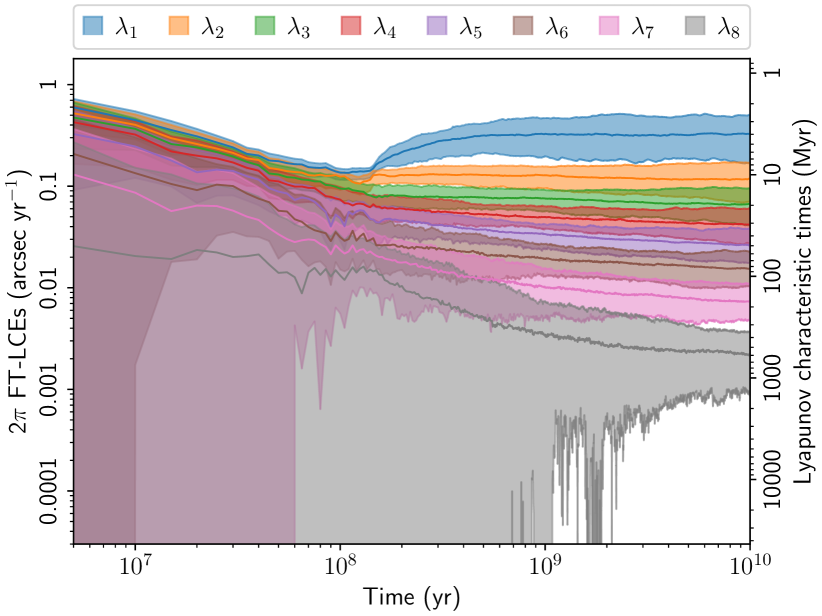
(a) $\mathcal{H}_{4}$

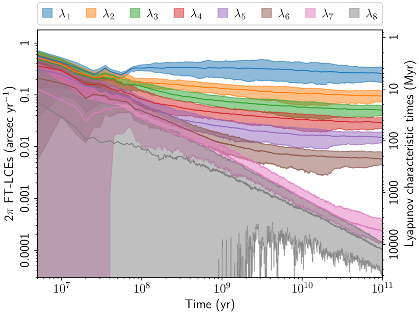
(b) $\mathbb{H}_{4}^{\bullet}$

ciao

Figure 1: Positive FT-LCEs $\lambda_{i}$ of the forced secular ISS from Hamiltonians $\mathcal{H}_{4}$ (a) and $\mathbb{H}_{4}^{\bullet}$ [Eq. (24)] (b), and corresponding characteristic timescales $\lambda_{i}^{-1}$. The bands represent the [5th, 95th] percentile range of the marginal PDFs estimated from an ensemble of 150 stable orbital solutions with very close initial conditions. The lines denote the distribution medians. The $\mathbb{H}_{4}^{\bullet}$ model is introduced and discussed in Sec. IV.4.

The FT-MLE of the forced secular ISS has been numerically computed over 5 Gyr for an ensemble of stable orbital solutions of the Hamiltonian $\mathcal{H}$ with initial conditions very close to their nominal values. Its long-term distribution is quite large and does not shrink over time [4, Fig. 3]. At 5 Gyr, the probability density function (PDF) of the Lyapunov time peaks at around 4 Myr, it decays very fast below 2 Myr, while its 99th percentile reaches 10 Myr [4, Fig. 4]. The significant width of the distribution relates to the aforementioned out-of-equilibrium dynamics of the ISS, as the FT-MLE of each orbital solution continues to vary over time. The dependence of the exponent on the initial condition is associated with the non-ergodic exploration of the phase space by the dynamics. As a remark, the fact that the lower tail of the FT-MLE distribution, estimated from more than 1000 solutions, does not extend to zero implies that invariant (KAM) tori are rare in a neighborhood of the nominal initial conditions (if they exist at all). This fact excludes that the dynamics is in a Nekhoroshev regime [39, 12], in agreement with the indications of a multidimensional resonance overlapping at the origin of chaos [40, 19]. In such a case, the long dynamical half-life of the ISS should not be interpreted in terms of an exponentially-slow Arnold diffusion.

Computations of the FT-MLE of the Solar System planets have been reported for more than thirty years [1, 3]. However, the retrieval of the entire spectrum of exponents still represents a challenging task. Integrating an $N$-body orbital solution for the Sun and the eight planets that spans 5 Gyr requires the order of a month of wall-clock time [e.g. 41]. The computation by a standard method of the entire Lyapunov spectrum for a system with $p$ d.o.f. also requires the simultaneous time evolution of a set of $2p$ tangent vectors [42]. On the top of that, a computation of the exponents for an ensemble of trajectories is advisable for a non-ergodic dynamics [4]. These considerations show how demanding the computation of the Lyapunov spectrum of the Solar System planets is. By contrast, a 5-Gyr integration of the forced ISS takes only a couple of hours for Gauss’s dynamics ($\mathcal{H}$) and a few minutes at degree 4 ($\mathcal{H}_{4}$). This dynamical model thus provides a unique opportunity to compute all the FT-LCEs that are mainly related to the secular evolution of the inner orbits.

We compute the Lyapunov spectrum of the truncated forced ISS using the standard method of Benettin et al. [43], based on Gram-Schmidt orthogonalization. Manipulation of the truncated Hamiltonian $\mathcal{H}_{2n}$ in TRIP allows us to systematically derive the equations of motion and the corresponding variational equations, which we integrate through an Adams PECE method of order 12 and a timestep of 250 years. Parallelization of the time evolution of the 16 tangent vectors, between two consecutive reorthonormalization steps of the Benettin et al. [43] algorithm, significantly reduces the computation time. Figure 1a shows the positive FT-LCEs expressed as angular frequencies over the next 10 Gyr for the Hamiltonian truncated at degree 4. The FT-LCEs are computed for 150 stable solutions, with initial conditions very close to the nominal values of Gauss’s dynamics and random sets of initial tangent vectors [19, Appendix C]. The figure shows the [5th, 95th] percentile range of the marginal PDF of each exponent estimated from the ensemble of solutions. For large times, the exponents of each solution become independent of the initial tangent vectors, the renormalization time, and the norm chosen for the phase-space vectors (see Appendix A and Fig. 7a). In this asymptotic regime, the Benettin et al. [43] algorithm purely retrieves the FT-LCEs as defined in Eq. (10), and the width of their distributions only reflects the out-of-equilibrium dynamics of the system. The convergence of our numerical computation is also assessed by verifying the symmetry of the spectrum stated in Eq. (9) (see Appendix A and Fig. 7b).

The spectrum in Fig. 1a has distinctive features. A set of intermediate exponents follow the MLE, ranging from 0.1 to 0.01${}^{\prime\prime}\,{\textrm{yr}}^{-1}$, while the smallest ones fall below 0.01${}^{\prime\prime}\,{\textrm{yr}}^{-1}$. Figure 1a reveals the existence of a hierarchy of exponents and corresponding timescales that spans two orders of magnitude, down to a median value of $\lambda_{8}^{-1}\approx 500$ Myr. The number of positive exponents confirms that no integral of motion exists, as one may expect from the forcing of the outer planets. We also compute the spectrum for the Hamiltonian truncated at degree 6. As shown in Appendix A (Fig. 9), the asymptotic distributions of the exponents are very similar to those at degree 4. This result suggests that long-term diffusion of the phase-space density is very close in the two cases. The different instability rates of the two truncated dynamics mainly relates to the geometry of the instability boundary, which is closer to the initial position of the system for $\mathcal{H}_{6}$ than for $\mathcal{H}_{4}$ [7].

The relevance of the Lyapunov spectrum in Fig. 1a emerges from the fact that the existence of an integral of motion implies a pair of vanishing exponents. This is a pivotal point: By a continuity argument, the presence of positive exponents much smaller than the leading one constitutes a compelling indication that there are dynamical quantities whose chaotic decoherence over initially very close trajectories takes place over timescales much longer than the Lyapunov time. In the long term, such quantities should diffuse much more slowly than any LL action variable. Therefore, Fig. 1a suggests that the secular orbits of the inner planets are characterized by a slow-fast dynamics that is much more pronounced than the well-known timescale separation arising from the LL integrable approximation. The existence of slow quantities, which are a priori complicated functions of the phase-space variables, is crucial in the context of finite-time stability, as they can effectively constrain the long-term diffusion of the phase-space density toward the unstable states. The next section addresses the emergence of these slow quantities from the symmetries of the Fourier harmonics that compose the Hamiltonian.

Table 2: Top of ranking $\mathcal{R}_{1}$. First 30 resonant harmonics of $\mathbb{H}_{10}$ along the 5-Gyr nominal solution of Gauss’s dynamics, in order of decreasing time median of the resonance half-width $\Delta\omega$ (${\textrm{arcsec yr}}^{-1}$). Adapted from Table 2 of Ref. [19].

$i$	Fourier harmonic $\mathcal{F}_{i}$	$\mathcal{O}_{i}$	$\tau_{i}^{\mathrm{res}}$	$\Delta\omega_{i}$
$1$	$g_{3}-g_{4}-s_{3}+s_{4}$	$4$	12%	${0.332}_{\mathchoice{\raisebox{2.0pt}{$\displaystyle\scriptscriptstyle 0.093$}}{\raisebox{2.0pt}{$\textstyle\scriptscriptstyle 0.093$}}{\raisebox{2.0pt}{$\scriptstyle\scriptscriptstyle 0.093$}}{\raisebox{2.0pt}{$\scriptscriptstyle\scriptscriptstyle 0.093$}}}^{\mathchoice{\raisebox{0.5pt}{$\displaystyle\scriptscriptstyle 0.526$}}{\raisebox{0.5pt}{$\textstyle\scriptscriptstyle 0.526$}}{\raisebox{0.5pt}{$\scriptstyle\scriptscriptstyle 0.526$}}{\raisebox{0.5pt}{$\scriptscriptstyle\scriptscriptstyle 0.526$}}}$
$2$	$g_{1}-g_{2}+s_{1}-s_{2}$	$4$	19%	${0.302}_{\mathchoice{\raisebox{2.0pt}{$\displaystyle\scriptscriptstyle 0.154$}}{\raisebox{2.0pt}{$\textstyle\scriptscriptstyle 0.154$}}{\raisebox{2.0pt}{$\scriptstyle\scriptscriptstyle 0.154$}}{\raisebox{2.0pt}{$\scriptscriptstyle\scriptscriptstyle 0.154$}}}^{\mathchoice{\raisebox{0.5pt}{$\displaystyle\scriptscriptstyle 0.611$}}{\raisebox{0.5pt}{$\textstyle\scriptscriptstyle 0.611$}}{\raisebox{0.5pt}{$\scriptstyle\scriptscriptstyle 0.611$}}{\raisebox{0.5pt}{$\scriptscriptstyle\scriptscriptstyle 0.611$}}}$
$3$	$g_{2}-g_{5}-2s_{1}+2s_{2}$	$6$	23%	${0.105}_{\mathchoice{\raisebox{2.0pt}{$\displaystyle\scriptscriptstyle 0.041$}}{\raisebox{2.0pt}{$\textstyle\scriptscriptstyle 0.041$}}{\raisebox{2.0pt}{$\scriptstyle\scriptscriptstyle 0.041$}}{\raisebox{2.0pt}{$\scriptscriptstyle\scriptscriptstyle 0.041$}}}^{\mathchoice{\raisebox{0.5pt}{$\displaystyle\scriptscriptstyle 0.223$}}{\raisebox{0.5pt}{$\textstyle\scriptscriptstyle 0.223$}}{\raisebox{0.5pt}{$\scriptstyle\scriptscriptstyle 0.223$}}{\raisebox{0.5pt}{$\scriptscriptstyle\scriptscriptstyle 0.223$}}}$
$4$	$2g_{3}-2g_{4}-s_{3}+s_{4}$	$6$	70%	${0.076}_{\mathchoice{\raisebox{2.0pt}{$\displaystyle\scriptscriptstyle 0.023$}}{\raisebox{2.0pt}{$\textstyle\scriptscriptstyle 0.023$}}{\raisebox{2.0pt}{$\scriptstyle\scriptscriptstyle 0.023$}}{\raisebox{2.0pt}{$\scriptscriptstyle\scriptscriptstyle 0.023$}}}^{\mathchoice{\raisebox{0.5pt}{$\displaystyle\scriptscriptstyle 0.159$}}{\raisebox{0.5pt}{$\textstyle\scriptscriptstyle 0.159$}}{\raisebox{0.5pt}{$\scriptstyle\scriptscriptstyle 0.159$}}{\raisebox{0.5pt}{$\scriptscriptstyle\scriptscriptstyle 0.159$}}}$
$5$	$g_{1}-g_{5}-s_{1}+s_{2}$	$4$	10%	${0.074}_{\mathchoice{\raisebox{2.0pt}{$\displaystyle\scriptscriptstyle 0.056$}}{\raisebox{2.0pt}{$\textstyle\scriptscriptstyle 0.056$}}{\raisebox{2.0pt}{$\scriptstyle\scriptscriptstyle 0.056$}}{\raisebox{2.0pt}{$\scriptscriptstyle\scriptscriptstyle 0.056$}}}^{\mathchoice{\raisebox{0.5pt}{$\displaystyle\scriptscriptstyle 0.178$}}{\raisebox{0.5pt}{$\textstyle\scriptscriptstyle 0.178$}}{\raisebox{0.5pt}{$\scriptstyle\scriptscriptstyle 0.178$}}{\raisebox{0.5pt}{$\scriptscriptstyle\scriptscriptstyle 0.178$}}}$
$6$	$g_{2}-g_{4}+s_{2}-s_{4}$	$4$	6%	${0.066}_{\mathchoice{\raisebox{2.0pt}{$\displaystyle\scriptscriptstyle 0.025$}}{\raisebox{2.0pt}{$\textstyle\scriptscriptstyle 0.025$}}{\raisebox{2.0pt}{$\scriptstyle\scriptscriptstyle 0.025$}}{\raisebox{2.0pt}{$\scriptscriptstyle\scriptscriptstyle 0.025$}}}^{\mathchoice{\raisebox{0.5pt}{$\displaystyle\scriptscriptstyle 0.098$}}{\raisebox{0.5pt}{$\textstyle\scriptscriptstyle 0.098$}}{\raisebox{0.5pt}{$\scriptstyle\scriptscriptstyle 0.098$}}{\raisebox{0.5pt}{$\scriptscriptstyle\scriptscriptstyle 0.098$}}}$
$7$	$g_{1}-2g_{2}+g_{4}+s_{1}-2s_{2}+s_{4}$	$8$	5%	${0.061}_{\mathchoice{\raisebox{2.0pt}{$\displaystyle\scriptscriptstyle 0.051$}}{\raisebox{2.0pt}{$\textstyle\scriptscriptstyle 0.051$}}{\raisebox{2.0pt}{$\scriptstyle\scriptscriptstyle 0.051$}}{\raisebox{2.0pt}{$\scriptscriptstyle\scriptscriptstyle 0.051$}}}^{\mathchoice{\raisebox{0.5pt}{$\displaystyle\scriptscriptstyle 0.074$}}{\raisebox{0.5pt}{$\textstyle\scriptscriptstyle 0.074$}}{\raisebox{0.5pt}{$\scriptstyle\scriptscriptstyle 0.074$}}{\raisebox{0.5pt}{$\scriptscriptstyle\scriptscriptstyle 0.074$}}}$
$8$	$g_{1}-g_{3}+s_{2}-s_{3}$	$4$	17%	${0.056}_{\mathchoice{\raisebox{2.0pt}{$\displaystyle\scriptscriptstyle 0.028$}}{\raisebox{2.0pt}{$\textstyle\scriptscriptstyle 0.028$}}{\raisebox{2.0pt}{$\scriptstyle\scriptscriptstyle 0.028$}}{\raisebox{2.0pt}{$\scriptscriptstyle\scriptscriptstyle 0.028$}}}^{\mathchoice{\raisebox{0.5pt}{$\displaystyle\scriptscriptstyle 0.090$}}{\raisebox{0.5pt}{$\textstyle\scriptscriptstyle 0.090$}}{\raisebox{0.5pt}{$\scriptstyle\scriptscriptstyle 0.090$}}{\raisebox{0.5pt}{$\scriptscriptstyle\scriptscriptstyle 0.090$}}}$
$9$	$g_{1}+g_{3}-2g_{4}+s_{2}-s_{3}$	$6$	5%	${0.053}_{\mathchoice{\raisebox{2.0pt}{$\displaystyle\scriptscriptstyle 0.037$}}{\raisebox{2.0pt}{$\textstyle\scriptscriptstyle 0.037$}}{\raisebox{2.0pt}{$\scriptstyle\scriptscriptstyle 0.037$}}{\raisebox{2.0pt}{$\scriptscriptstyle\scriptscriptstyle 0.037$}}}^{\mathchoice{\raisebox{0.5pt}{$\displaystyle\scriptscriptstyle 0.061$}}{\raisebox{0.5pt}{$\textstyle\scriptscriptstyle 0.061$}}{\raisebox{0.5pt}{$\scriptstyle\scriptscriptstyle 0.061$}}{\raisebox{0.5pt}{$\scriptscriptstyle\scriptscriptstyle 0.061$}}}$
$10$	$3g_{3}-3g_{4}-s_{3}+s_{4}$	$8$	9%	${0.052}_{\mathchoice{\raisebox{2.0pt}{$\displaystyle\scriptscriptstyle 0.007$}}{\raisebox{2.0pt}{$\textstyle\scriptscriptstyle 0.007$}}{\raisebox{2.0pt}{$\scriptstyle\scriptscriptstyle 0.007$}}{\raisebox{2.0pt}{$\scriptscriptstyle\scriptscriptstyle 0.007$}}}^{\mathchoice{\raisebox{0.5pt}{$\displaystyle\scriptscriptstyle 0.140$}}{\raisebox{0.5pt}{$\textstyle\scriptscriptstyle 0.140$}}{\raisebox{0.5pt}{$\scriptstyle\scriptscriptstyle 0.140$}}{\raisebox{0.5pt}{$\scriptscriptstyle\scriptscriptstyle 0.140$}}}$
$11$	$g_{2}-g_{3}-s_{1}+2s_{2}-s_{3}$	$6$	5%	${0.038}_{\mathchoice{\raisebox{2.0pt}{$\displaystyle\scriptscriptstyle 0.028$}}{\raisebox{2.0pt}{$\textstyle\scriptscriptstyle 0.028$}}{\raisebox{2.0pt}{$\scriptstyle\scriptscriptstyle 0.028$}}{\raisebox{2.0pt}{$\scriptscriptstyle\scriptscriptstyle 0.028$}}}^{\mathchoice{\raisebox{0.5pt}{$\displaystyle\scriptscriptstyle 0.047$}}{\raisebox{0.5pt}{$\textstyle\scriptscriptstyle 0.047$}}{\raisebox{0.5pt}{$\scriptstyle\scriptscriptstyle 0.047$}}{\raisebox{0.5pt}{$\scriptscriptstyle\scriptscriptstyle 0.047$}}}$
$12$	$g_{1}-2g_{3}+g_{4}+s_{2}-s_{4}$	$6$	36%	${0.038}_{\mathchoice{\raisebox{2.0pt}{$\displaystyle\scriptscriptstyle 0.016$}}{\raisebox{2.0pt}{$\textstyle\scriptscriptstyle 0.016$}}{\raisebox{2.0pt}{$\scriptstyle\scriptscriptstyle 0.016$}}{\raisebox{2.0pt}{$\scriptscriptstyle\scriptscriptstyle 0.016$}}}^{\mathchoice{\raisebox{0.5pt}{$\displaystyle\scriptscriptstyle 0.083$}}{\raisebox{0.5pt}{$\textstyle\scriptscriptstyle 0.083$}}{\raisebox{0.5pt}{$\scriptstyle\scriptscriptstyle 0.083$}}{\raisebox{0.5pt}{$\scriptscriptstyle\scriptscriptstyle 0.083$}}}$
$13$	$2g_{1}-g_{3}-g_{5}+s_{2}-s_{4}$	$6$	5%	${0.037}_{\mathchoice{\raisebox{2.0pt}{$\displaystyle\scriptscriptstyle 0.028$}}{\raisebox{2.0pt}{$\textstyle\scriptscriptstyle 0.028$}}{\raisebox{2.0pt}{$\scriptstyle\scriptscriptstyle 0.028$}}{\raisebox{2.0pt}{$\scriptscriptstyle\scriptscriptstyle 0.028$}}}^{\mathchoice{\raisebox{0.5pt}{$\displaystyle\scriptscriptstyle 0.043$}}{\raisebox{0.5pt}{$\textstyle\scriptscriptstyle 0.043$}}{\raisebox{0.5pt}{$\scriptstyle\scriptscriptstyle 0.043$}}{\raisebox{0.5pt}{$\scriptscriptstyle\scriptscriptstyle 0.043$}}}$
$14$	$g_{4}-g_{5}-s_{2}+2s_{3}-s_{4}$	$6$	2%	${0.033}_{\mathchoice{\raisebox{2.0pt}{$\displaystyle\scriptscriptstyle 0.031$}}{\raisebox{2.0pt}{$\textstyle\scriptscriptstyle 0.031$}}{\raisebox{2.0pt}{$\scriptstyle\scriptscriptstyle 0.031$}}{\raisebox{2.0pt}{$\scriptscriptstyle\scriptscriptstyle 0.031$}}}^{\mathchoice{\raisebox{0.5pt}{$\displaystyle\scriptscriptstyle 0.036$}}{\raisebox{0.5pt}{$\textstyle\scriptscriptstyle 0.036$}}{\raisebox{0.5pt}{$\scriptstyle\scriptscriptstyle 0.036$}}{\raisebox{0.5pt}{$\scriptscriptstyle\scriptscriptstyle 0.036$}}}$
$15$	$g_{1}-2g_{3}+g_{4}+s_{1}+s_{3}-2s_{4}$	$8$	25%	${0.033}_{\mathchoice{\raisebox{2.0pt}{$\displaystyle\scriptscriptstyle 0.014$}}{\raisebox{2.0pt}{$\textstyle\scriptscriptstyle 0.014$}}{\raisebox{2.0pt}{$\scriptstyle\scriptscriptstyle 0.014$}}{\raisebox{2.0pt}{$\scriptscriptstyle\scriptscriptstyle 0.014$}}}^{\mathchoice{\raisebox{0.5pt}{$\displaystyle\scriptscriptstyle 0.045$}}{\raisebox{0.5pt}{$\textstyle\scriptscriptstyle 0.045$}}{\raisebox{0.5pt}{$\scriptstyle\scriptscriptstyle 0.045$}}{\raisebox{0.5pt}{$\scriptscriptstyle\scriptscriptstyle 0.045$}}}$
$16$	$g_{1}-g_{4}+s_{1}-s_{4}$	$4$	23%	${0.032}_{\mathchoice{\raisebox{2.0pt}{$\displaystyle\scriptscriptstyle 0.017$}}{\raisebox{2.0pt}{$\textstyle\scriptscriptstyle 0.017$}}{\raisebox{2.0pt}{$\scriptstyle\scriptscriptstyle 0.017$}}{\raisebox{2.0pt}{$\scriptscriptstyle\scriptscriptstyle 0.017$}}}^{\mathchoice{\raisebox{0.5pt}{$\displaystyle\scriptscriptstyle 0.054$}}{\raisebox{0.5pt}{$\textstyle\scriptscriptstyle 0.054$}}{\raisebox{0.5pt}{$\scriptstyle\scriptscriptstyle 0.054$}}{\raisebox{0.5pt}{$\scriptscriptstyle\scriptscriptstyle 0.054$}}}$
$17$	$g_{1}-2g_{2}+g_{5}+3s_{1}-3s_{2}$	$10$	6%	${0.032}_{\mathchoice{\raisebox{2.0pt}{$\displaystyle\scriptscriptstyle 0.023$}}{\raisebox{2.0pt}{$\textstyle\scriptscriptstyle 0.023$}}{\raisebox{2.0pt}{$\scriptstyle\scriptscriptstyle 0.023$}}{\raisebox{2.0pt}{$\scriptscriptstyle\scriptscriptstyle 0.023$}}}^{\mathchoice{\raisebox{0.5pt}{$\displaystyle\scriptscriptstyle 0.039$}}{\raisebox{0.5pt}{$\textstyle\scriptscriptstyle 0.039$}}{\raisebox{0.5pt}{$\scriptstyle\scriptscriptstyle 0.039$}}{\raisebox{0.5pt}{$\scriptscriptstyle\scriptscriptstyle 0.039$}}}$
$18$	$g_{1}-g_{4}+s_{2}-s_{3}$	$4$	18%	${0.031}_{\mathchoice{\raisebox{2.0pt}{$\displaystyle\scriptscriptstyle 0.016$}}{\raisebox{2.0pt}{$\textstyle\scriptscriptstyle 0.016$}}{\raisebox{2.0pt}{$\scriptstyle\scriptscriptstyle 0.016$}}{\raisebox{2.0pt}{$\scriptscriptstyle\scriptscriptstyle 0.016$}}}^{\mathchoice{\raisebox{0.5pt}{$\displaystyle\scriptscriptstyle 0.073$}}{\raisebox{0.5pt}{$\textstyle\scriptscriptstyle 0.073$}}{\raisebox{0.5pt}{$\scriptstyle\scriptscriptstyle 0.073$}}{\raisebox{0.5pt}{$\scriptscriptstyle\scriptscriptstyle 0.073$}}}$
$19$	$3g_{1}-g_{2}-g_{4}-g_{5}+s_{1}-s_{3}$	$8$	2%	${0.031}_{\mathchoice{\raisebox{2.0pt}{$\displaystyle\scriptscriptstyle 0.023$}}{\raisebox{2.0pt}{$\textstyle\scriptscriptstyle 0.023$}}{\raisebox{2.0pt}{$\scriptstyle\scriptscriptstyle 0.023$}}{\raisebox{2.0pt}{$\scriptscriptstyle\scriptscriptstyle 0.023$}}}^{\mathchoice{\raisebox{0.5pt}{$\displaystyle\scriptscriptstyle 0.042$}}{\raisebox{0.5pt}{$\textstyle\scriptscriptstyle 0.042$}}{\raisebox{0.5pt}{$\scriptstyle\scriptscriptstyle 0.042$}}{\raisebox{0.5pt}{$\scriptscriptstyle\scriptscriptstyle 0.042$}}}$
$20$	$2g_{1}-g_{2}-g_{3}+s_{1}-s_{3}$	$6$	29%	${0.028}_{\mathchoice{\raisebox{2.0pt}{$\displaystyle\scriptscriptstyle 0.016$}}{\raisebox{2.0pt}{$\textstyle\scriptscriptstyle 0.016$}}{\raisebox{2.0pt}{$\scriptstyle\scriptscriptstyle 0.016$}}{\raisebox{2.0pt}{$\scriptscriptstyle\scriptscriptstyle 0.016$}}}^{\mathchoice{\raisebox{0.5pt}{$\displaystyle\scriptscriptstyle 0.051$}}{\raisebox{0.5pt}{$\textstyle\scriptscriptstyle 0.051$}}{\raisebox{0.5pt}{$\scriptstyle\scriptscriptstyle 0.051$}}{\raisebox{0.5pt}{$\scriptscriptstyle\scriptscriptstyle 0.051$}}}$
$21$	$2g_{1}-g_{2}-g_{4}+s_{1}-s_{3}$	$6$	3%	${0.026}_{\mathchoice{\raisebox{2.0pt}{$\displaystyle\scriptscriptstyle 0.021$}}{\raisebox{2.0pt}{$\textstyle\scriptscriptstyle 0.021$}}{\raisebox{2.0pt}{$\scriptstyle\scriptscriptstyle 0.021$}}{\raisebox{2.0pt}{$\scriptscriptstyle\scriptscriptstyle 0.021$}}}^{\mathchoice{\raisebox{0.5pt}{$\displaystyle\scriptscriptstyle 0.028$}}{\raisebox{0.5pt}{$\textstyle\scriptscriptstyle 0.028$}}{\raisebox{0.5pt}{$\scriptstyle\scriptscriptstyle 0.028$}}{\raisebox{0.5pt}{$\scriptscriptstyle\scriptscriptstyle 0.028$}}}$
$22$	$3g_{3}-3g_{4}-2s_{3}+2s_{4}$	$10$	8%	${0.025}_{\mathchoice{\raisebox{2.0pt}{$\displaystyle\scriptscriptstyle 0.012$}}{\raisebox{2.0pt}{$\textstyle\scriptscriptstyle 0.012$}}{\raisebox{2.0pt}{$\scriptstyle\scriptscriptstyle 0.012$}}{\raisebox{2.0pt}{$\scriptscriptstyle\scriptscriptstyle 0.012$}}}^{\mathchoice{\raisebox{0.5pt}{$\displaystyle\scriptscriptstyle 0.055$}}{\raisebox{0.5pt}{$\textstyle\scriptscriptstyle 0.055$}}{\raisebox{0.5pt}{$\scriptstyle\scriptscriptstyle 0.055$}}{\raisebox{0.5pt}{$\scriptscriptstyle\scriptscriptstyle 0.055$}}}$
$23$	$2g_{1}-g_{2}-2g_{3}+g_{4}+s_{1}-s_{4}$	$8$	3%	${0.023}_{\mathchoice{\raisebox{2.0pt}{$\displaystyle\scriptscriptstyle 0.012$}}{\raisebox{2.0pt}{$\textstyle\scriptscriptstyle 0.012$}}{\raisebox{2.0pt}{$\scriptstyle\scriptscriptstyle 0.012$}}{\raisebox{2.0pt}{$\scriptscriptstyle\scriptscriptstyle 0.012$}}}^{\mathchoice{\raisebox{0.5pt}{$\displaystyle\scriptscriptstyle 0.036$}}{\raisebox{0.5pt}{$\textstyle\scriptscriptstyle 0.036$}}{\raisebox{0.5pt}{$\scriptstyle\scriptscriptstyle 0.036$}}{\raisebox{0.5pt}{$\scriptscriptstyle\scriptscriptstyle 0.036$}}}$
$24$	$2g_{3}-g_{4}-g_{5}-s_{1}+s_{4}$	$6$	16%	${0.023}_{\mathchoice{\raisebox{2.0pt}{$\displaystyle\scriptscriptstyle 0.010$}}{\raisebox{2.0pt}{$\textstyle\scriptscriptstyle 0.010$}}{\raisebox{2.0pt}{$\scriptstyle\scriptscriptstyle 0.010$}}{\raisebox{2.0pt}{$\scriptscriptstyle\scriptscriptstyle 0.010$}}}^{\mathchoice{\raisebox{0.5pt}{$\displaystyle\scriptscriptstyle 0.048$}}{\raisebox{0.5pt}{$\textstyle\scriptscriptstyle 0.048$}}{\raisebox{0.5pt}{$\scriptstyle\scriptscriptstyle 0.048$}}{\raisebox{0.5pt}{$\scriptscriptstyle\scriptscriptstyle 0.048$}}}$
$25$	$g_{1}-3g_{3}+2g_{4}+s_{2}-s_{4}$	$8$	7%	${0.021}_{\mathchoice{\raisebox{2.0pt}{$\displaystyle\scriptscriptstyle 0.008$}}{\raisebox{2.0pt}{$\textstyle\scriptscriptstyle 0.008$}}{\raisebox{2.0pt}{$\scriptstyle\scriptscriptstyle 0.008$}}{\raisebox{2.0pt}{$\scriptscriptstyle\scriptscriptstyle 0.008$}}}^{\mathchoice{\raisebox{0.5pt}{$\displaystyle\scriptscriptstyle 0.030$}}{\raisebox{0.5pt}{$\textstyle\scriptscriptstyle 0.030$}}{\raisebox{0.5pt}{$\scriptstyle\scriptscriptstyle 0.030$}}{\raisebox{0.5pt}{$\scriptscriptstyle\scriptscriptstyle 0.030$}}}$
$26$	$g_{1}-g_{2}-g_{3}+g_{4}+s_{1}-s_{2}$	$6$	6%	${0.021}_{\mathchoice{\raisebox{2.0pt}{$\displaystyle\scriptscriptstyle 0.004$}}{\raisebox{2.0pt}{$\textstyle\scriptscriptstyle 0.004$}}{\raisebox{2.0pt}{$\scriptstyle\scriptscriptstyle 0.004$}}{\raisebox{2.0pt}{$\scriptscriptstyle\scriptscriptstyle 0.004$}}}^{\mathchoice{\raisebox{0.5pt}{$\displaystyle\scriptscriptstyle 0.032$}}{\raisebox{0.5pt}{$\textstyle\scriptscriptstyle 0.032$}}{\raisebox{0.5pt}{$\scriptstyle\scriptscriptstyle 0.032$}}{\raisebox{0.5pt}{$\scriptscriptstyle\scriptscriptstyle 0.032$}}}$
$27$	$g_{1}+g_{3}-2g_{4}+s_{1}-s_{4}$	$6$	3%	${0.021}_{\mathchoice{\raisebox{2.0pt}{$\displaystyle\scriptscriptstyle 0.017$}}{\raisebox{2.0pt}{$\textstyle\scriptscriptstyle 0.017$}}{\raisebox{2.0pt}{$\scriptstyle\scriptscriptstyle 0.017$}}{\raisebox{2.0pt}{$\scriptscriptstyle\scriptscriptstyle 0.017$}}}^{\mathchoice{\raisebox{0.5pt}{$\displaystyle\scriptscriptstyle 0.022$}}{\raisebox{0.5pt}{$\textstyle\scriptscriptstyle 0.022$}}{\raisebox{0.5pt}{$\scriptstyle\scriptscriptstyle 0.022$}}{\raisebox{0.5pt}{$\scriptscriptstyle\scriptscriptstyle 0.022$}}}$
$28$	$g_{1}+g_{2}-2g_{5}-3s_{1}+3s_{2}$	$10$	4%	${0.020}_{\mathchoice{\raisebox{2.0pt}{$\displaystyle\scriptscriptstyle 0.006$}}{\raisebox{2.0pt}{$\textstyle\scriptscriptstyle 0.006$}}{\raisebox{2.0pt}{$\scriptstyle\scriptscriptstyle 0.006$}}{\raisebox{2.0pt}{$\scriptscriptstyle\scriptscriptstyle 0.006$}}}^{\mathchoice{\raisebox{0.5pt}{$\displaystyle\scriptscriptstyle 0.028$}}{\raisebox{0.5pt}{$\textstyle\scriptscriptstyle 0.028$}}{\raisebox{0.5pt}{$\scriptstyle\scriptscriptstyle 0.028$}}{\raisebox{0.5pt}{$\scriptscriptstyle\scriptscriptstyle 0.028$}}}$
$29$	$3g_{1}-g_{2}-g_{4}-g_{5}+s_{2}-s_{3}$	$8$	4%	${0.020}_{\mathchoice{\raisebox{2.0pt}{$\displaystyle\scriptscriptstyle 0.008$}}{\raisebox{2.0pt}{$\textstyle\scriptscriptstyle 0.008$}}{\raisebox{2.0pt}{$\scriptstyle\scriptscriptstyle 0.008$}}{\raisebox{2.0pt}{$\scriptscriptstyle\scriptscriptstyle 0.008$}}}^{\mathchoice{\raisebox{0.5pt}{$\displaystyle\scriptscriptstyle 0.027$}}{\raisebox{0.5pt}{$\textstyle\scriptscriptstyle 0.027$}}{\raisebox{0.5pt}{$\scriptstyle\scriptscriptstyle 0.027$}}{\raisebox{0.5pt}{$\scriptscriptstyle\scriptscriptstyle 0.027$}}}$
$30$	$2g_{1}-g_{4}-g_{5}+s_{2}-s_{4}$	$6$	7%	${0.020}_{\mathchoice{\raisebox{2.0pt}{$\displaystyle\scriptscriptstyle 0.007$}}{\raisebox{2.0pt}{$\textstyle\scriptscriptstyle 0.007$}}{\raisebox{2.0pt}{$\scriptstyle\scriptscriptstyle 0.007$}}{\raisebox{2.0pt}{$\scriptscriptstyle\scriptscriptstyle 0.007$}}}^{\mathchoice{\raisebox{0.5pt}{$\displaystyle\scriptscriptstyle 0.029$}}{\raisebox{0.5pt}{$\textstyle\scriptscriptstyle 0.029$}}{\raisebox{0.5pt}{$\scriptstyle\scriptscriptstyle 0.029$}}{\raisebox{0.5pt}{$\scriptscriptstyle\scriptscriptstyle 0.029$}}}$

IV Quasi-integrals of motion

The emergence of a chaotic behavior of the planetary orbits can be explained in terms of the pendulum-like dynamics generated by each Fourier harmonic that composes the Hamiltonian in Eq. (6) [e.g. 44]. One can write $\mathbb{H}_{2n}(\bm{I},\bm{\theta},t)=\widetilde{\mathbb{H}}_{2n}^{\bm{0},\bm{0}}(\bm{I})+\sum_{i=1}^{\mathcal{M}_{2n}}\mathcal{F}_{i}(\bm{I},\bm{\theta},t)$, with

$$\mathcal{F}_{i}(\bm{I},\bm{\theta},t)=\widetilde{\mathbb{H}}_{2n}^{\bm{k}^{i}\!,\bm{\ell}^{i}}\!(\bm{I})\,\mathrm{E}^{j\left(\bm{k}^{i}\cdot\bm{\theta}+\bm{\ell}^{i}\cdot\bm{\phi}(t)\right)}+\mathrm{c.c.},$$ (11)

where $(\bm{k}^{i},\bm{\ell}^{i})\neq(\bm{0},\bm{0})$, $\mathcal{M}_{2n}$ is the number of harmonics in $\mathbb{H}_{2n}$ with a non-null wave vector, and $\mathrm{c.c.}$ stands for complex conjugate. Chaos arises from the interaction of resonant harmonics, that is, those harmonics $\mathcal{F}_{i}$ whose frequency combination $\bm{k}^{i}\cdot\dot{\bm{\theta}}+\bm{\ell}^{i}\cdot\dot{\bm{\phi}}(t)$ vanishes at some point along the motion. Using the computer algebra system TRIP, the harmonics of $\mathbb{H}_{10}$ that enter into resonance along the 5-Gyr nominal solution of Gauss’s dynamics have been systematically retrieved, together with the corresponding time statistics of the resonance half-widths $\Delta\omega$ [19]. The resonances have then been ordered by decreasing time median of their half-widths. The resulting ranking of resonances is denoted as $\mathcal{R}_{1}$ from now on. Table III recalls the 30 strongest resonances that are active for more than 1% of the 5-Gyr time span of the orbital solution. The wave vector of each harmonic is identified by the corresponding combination of frequency labels $(g_{i},s_{i})_{i=1}^{8}$, that is, $\bm{k}\cdot\bm{\omega}_{\textnormal{\scriptsize i}}+\bm{\ell}\cdot\bm{\omega}_{\textnormal{\scriptsize o}}$, with $\bm{\omega}_{\textnormal{\scriptsize i}}=(g_{1},g_{2},g_{3},g_{4},s_{1},s_{2},s_{3},s_{4})$. Table III also shows the order of each harmonic, defined as the even integer $\mathcal{O}=\|(\bm{k},\bm{\ell})\|_{1}$. The support of the asymptotic ensemble distribution of the FT-MLE shown in Fig. 1a overlaps in a robust way with that of the time distribution of the half-width of the strongest resonances. In other words,

$$2\pi\lambda_{1}\approx\Delta\omega^{\mathcal{R}_{1}},$$ (12)

where $\Delta\omega^{\mathcal{R}_{1}}$ stands for the half-width of the uppermost resonances of ranking $\mathcal{R}_{1}$. Equation (12) shows the dynamical sources of chaos in the ISS by connecting the top of the Lyapunov spectrum with the head of the resonance spectrum. Computer algebra allows us to establish such a connection in an unbiased way despite the multidimensional nature of the dynamics. We stress that such analysis is built on the idea that the time statistics of the resonant harmonics along a 5-Gyr ordinary orbital solution should be representative of their ensemble statistics (defined by a set of stable solutions with very close initial conditions) at some large time of the order of billions of years. This assumption was inspired by the good level of stationarity that characterizes the ensemble distribution of the MLE beyond 1 Gyr [4, 19], and that extends to the entire spectrum in Fig. 1a.

We remark that, strictly speaking, ranking $\mathcal{R}_{1}$ is established on the Fourier harmonics of the Lie-transformed Hamiltonian $\mathbb{H}_{2n}^{\prime}$ [19, Appendix G]. New canonical variables are indeed defined to transform $\mathbb{H}_{2n}$ in a Birkhoff normal form to degree 4. The goal is to let the interactions of the terms of degree 4 in $\mathbb{H}_{2n}$ appear more explicitly in the amplitudes of the harmonics of higher degrees in $\mathbb{H}_{2n}^{\prime}$, the physical motivation being that the non-linear interaction of the harmonics at degree 4 constitutes the primary source of chaos [19]. Keeping in mind the quasi-identity nature of the Lie transform, here we drop for simplicity the difference between the two Hamiltonians. Moreover, all the new analyses of this work involve the original variables of Eq. (5).

IV.1 Quasi-symmetries of the resonant harmonics

In addition to the dynamical interactions responsible for the chaotic behavior of the orbits, Table III provides information on the geometry of the dynamics in the action variable space. Ranking the Fourier harmonics allows us to consider partial Hamiltonians constructed from a limited number $m$ of leading terms [19, 7], that is,

$$\mathbb{H}_{2n,m}=\widetilde{\mathbb{H}}_{2n}^{\bm{0},\bm{0}}+\textstyle{\sum_{i=1}^{m}}\mathcal{F}_{i}.$$ (13)

The dynamics of a Hamiltonian reduced to a small set of harmonics is generally characterized by several symmetries and corresponding integrals of motion. We are interested in how these symmetries are progressively destroyed when one increases the number of terms taken into account in Eq. (13).

Consider a set of $m$ harmonics of $\mathbb{H}_{2n}$ and a dynamical quantity that is a linear combination of the action variables, that is,

$$C_{\bm{\gamma}}=\bm{\gamma}\cdot\bm{I},$$ (14)

$\bm{\gamma}\in\mathbb{R}^{8}$ being a parameter vector. From Eq. (11), the partial contribution of the $m$ harmonics to the time derivative of $C_{\bm{\gamma}}$ along the flow of $\mathbb{H}_{2n}$ is

$$\dot{C}_{\bm{\gamma},m}=2\sum_{i=1}^{m}\bm{\gamma}\cdot\bm{k}^{i}\operatorname{Im}\{\widetilde{\mathbb{H}}_{2n}^{\bm{k}^{i}\!,\bm{\ell}^{i}}\!(\bm{I})\,\mathrm{E}^{j\left(\bm{k}^{i}\cdot\bm{\theta}+\bm{\ell}^{i}\cdot\bm{\phi}(t)\right)}\},$$ (15)

and $\dot{C}_{\bm{\gamma}}=\dot{C}_{\bm{\gamma},\mathcal{M}_{2n}}$, where $\mathcal{M}_{2n}$ is the total number of harmonics with a non-null wave vector that appear in $\mathbb{H}_{2n}$. Any quantity $C_{\bm{\gamma}}$ with $\bm{\gamma}\cdot\bm{k}^{i}=0$ is conserved by the one-d.o.f. dynamics generated by the single harmonic $\mathcal{F}_{i}$. In other words, such a quantity would be an integral of motion if $\mathcal{F}_{i}$ were the only harmonic to appear in the Hamiltonian. Considering now $m$ different harmonics, these do not contribute to the change of the quantity $C_{\bm{\gamma}}$ if $\bm{\gamma}\perp\operatorname{span}(\bm{k}^{1},\bm{k}^{2},\dots,\bm{k}^{m})$, that is, if the vector $\bm{\gamma}$ belongs to the orthogonal complement of the linear subspace of $\mathbb{R}^{8}$ spanned by the wave vectors $(\bm{k}^{i})_{i=1}^{m}$. We also consider the quantity

$$C_{\bm{\gamma}}^{\prime}=\mathbb{H}_{2n}+\bm{\gamma}\cdot\bm{I}.$$ (16)

Because of the explicit time dependence in the Hamiltonian, the partial contribution of a set of $m$ harmonics to the time derivative of $C_{\bm{\gamma}}^{\prime}$ along the flow of $\mathbb{H}_{2n}$ is

$$\dot{C}^{\prime}_{\bm{\gamma},m}=2\sum_{i=1}^{m}(\bm{\gamma}\cdot\bm{k}^{i}+\bm{\ell}^{i}\cdot\bm{\omega}_{\textnormal{\scriptsize o}})\operatorname{Im}\{\widetilde{\mathbb{H}}_{2n}^{\bm{k}^{i}\!,\bm{\ell}^{i}}\!(\bm{I})\,\mathrm{E}^{j\left(\bm{k}^{i}\cdot\bm{\theta}+\bm{\ell}^{i}\cdot\bm{\phi}(t)\right)}\},$$ (17)

and one has $\dot{C}^{\prime}_{\bm{\gamma}}=\dot{C}^{\prime}_{\bm{\gamma},\mathcal{M}_{2n}}$. Quantity $C_{\bm{\gamma}}^{\prime}$ is unchanged by the $m$ harmonics if $\bm{\gamma}\cdot\bm{k}^{i}+\bm{\ell}^{i}\cdot\bm{\omega}_{\textnormal{\scriptsize o}}=0$ for $i\in\{1,2,\dots,m\}$. Dynamical quantities $C_{\bm{\gamma}}$ or $C^{\prime}_{\bm{\gamma}}$ that are unaffected by a given set of leading harmonics, that is, with null partial contribution in Eq. (15) or (17), are denoted as quasi-integrals of motion from now on. More specifically, we build our analysis on ranking $\mathcal{R}_{1}$, since the resonant harmonics are those responsible for changes that accumulate stochastically over long timescales, driving chaotic diffusion.

In the framework of the aforementioned considerations, the resonances listed in Table III possess three different symmetries.

First symmetry.

The rotational invariance of the entire Solar System implies the d’Alembert rule $\sum_{i=1}^{8}k_{i}+\sum_{i=1}^{7}\ell_{i}=0$, where $\bm{k}=(k_{1},k_{2},\dots,k_{8})$ and $\bm{\ell}=(\ell_{1},\ell_{2},\dots,\ell_{7})$ [45, 24, 21, 46]. Moreover, the Jupiter-dominated eccentricity mode $g_{5}$ is the only fundamental Fourier mode of the outer planet forcing to appear in Table III. The quantity

$$\mathcal{E}_{2n}\vcentcolon=C_{g_{5}\bm{1}_{8}}^{\prime}=\mathbb{H}_{2n}+g_{5}\textstyle{\sum_{i=1}^{4}}(\mathfrak{X}_{i}+\Psi_{i}),$$ (18)

with $\bm{1}_{8}=(1,1,\dots,1)\in\mathbb{R}^{8}$, is therefore unaffected by the resonances listed in Table III. In an equivalent way, the time-dependent canonical transformation $\bm{\theta}\rightarrow\bm{\theta}+g_{5}t\,\bm{1}_{8}$, with unchanged action variables, allows us to remove the explicit time dependence in these harmonics. Quantity $\mathcal{E}_{2n}$ coincides with the transformed Hamiltonian and the harmonics in Table III do not contribute to its time derivative.

Second symmetry.

We write the eccentricity and inclination parts of the harmonic wave vectors explicitly, that is, $\bm{k}=(\bm{k}^{\textnormal{\scriptsize ecc}},\bm{k}^{\textnormal{\scriptsize inc}})$ with $\bm{k}^{\textnormal{\scriptsize ecc}},\bm{k}^{\textnormal{\scriptsize inc}}\in\mathbb{R}^{4}$. One can visually check that the harmonics in Table III verify the relation $\sum_{i=1}^{4}k^{\textnormal{\scriptsize inc}}_{i}=0$, where $\bm{k}^{\textnormal{\scriptsize inc}}~{}=~{}(k^{\textnormal{\scriptsize inc}}_{1},\dots,k^{\textnormal{\scriptsize inc}}_{4})$. Therefore, denoting $\bm{\gamma}_{1}=(\bm{0}_{4},\bm{1}_{4})$, the quantity

$$\mathcal{C}_{\textnormal{\scriptsize inc}}\vcentcolon=C_{\bm{\gamma}_{1}}=\Psi_{1}+\Psi_{2}+\Psi_{3}+\Psi_{4}$$ (19)

is conserved by these resonances. $\mathcal{C}_{\textnormal{\scriptsize inc}}$ is the angular momentum deficit (AMD) [47] contained in the inclination d.o.f. This symmetry can then be interpreted as a remnant of the conservation of the AMD of the entire (secular) Solar System. We remark that the AMD contained in the eccentricity d.o.f., $\mathcal{C}_{\textnormal{\scriptsize ecc}}=\sum_{i=1}^{4}\mathfrak{X}_{i}$, is not invariant under the leading resonances because of the eccentricity forcing mainly exerted by Jupiter through the mode $g_{5}$. The conservation of $\mathcal{C}_{\textnormal{\scriptsize inc}}$ depends on two facts: the inclination modes $s_{6},s_{7},s_{8}$ of the external forcing do not appear in Table III; low-order harmonics like $2g_{1}-s_{1}-s_{2}$, $2g_{1}-2s_{1}$, and $2g_{1}-2s_{2}$ are never resonant (even if they can raise large quasi-periodic contributions), so that two AMD reservoirs $\mathcal{C}_{\textnormal{\scriptsize ecc}}$ and $\mathcal{C}_{\textnormal{\scriptsize inc}}$ are decoupled in Table III. We recall that the absence of an inclination mode $s_{5}$ in the external forcing relates to the fixed direction of the angular momentum of the entire Solar System [2, 21, 46].

Third symmetry.

The first two symmetries could be expected to some extent on the basis of physical intuition of the interaction between outer and inner planets. However, it is not easy to even visually guess the third one from Table III. Consider the $30\times 8$ matrix $\mathbf{K}_{30}$ whose rows are the wave vectors $(\bm{k}^{i})_{i=1}^{30}$ of the listed resonances. A singular value decomposition shows that the rank of $\mathbf{K}_{30}$ is equal to 6. Therefore, the linear subspace $V_{30}=\operatorname{span}(\bm{k}^{1},\bm{k}^{2},\dots,\bm{k}^{30})$ spanned by the wave vectors has dimension 6. A Gram–Schmidt orthogonalization allows us to determine two linearly independent vectors that span its orthogonal complement $V_{30}^{\perp}$. One choice consists in $V_{30}^{\perp}=\operatorname{span}(\bm{\gamma}_{2},\bm{\gamma}_{2}^{\perp})$, with

$$\mathcal{C}_{2}\vcentcolon=\mathcal{C}_{\bm{\gamma}_{2}} =-\mathfrak{X}_{3}-\mathfrak{X}_{4}+\Psi_{1}+\Psi_{2}+2\Psi_{3}+2\Psi_{4},$$ (20)

$$\mathcal{C}_{2}^{\perp}\vcentcolon=\mathcal{C}_{\bm{\gamma}_{2}^{\perp}} =\phantom{-}\mathfrak{X}_{3}+\mathfrak{X}_{4}+\Psi_{1}+\Psi_{2}.$$

Since the second symmetry clearly requires that $\bm{\gamma}_{1}\in V_{30}^{\perp}$, the three quantities $\mathcal{C}_{\textnormal{\scriptsize inc}},\mathcal{C}_{2},\mathcal{C}_{2}^{\perp}$ are not independent and one has indeed $\mathcal{C}_{\textnormal{\scriptsize inc}}=(\mathcal{C}_{2}+\mathcal{C}_{2}^{\perp})/2$. We remark that $(\mathcal{C}_{2}-\mathcal{C}_{2}^{\perp})/2=-\mathfrak{X}_{3}-\mathfrak{X}_{4}+\Psi_{3}+\Psi_{4}$. The additional symmetry can thus be interpreted in terms of a certain decoupling between the d.o.f. 3, 4 and 1, 2, representing in the proper modes the Earth-Mars and Mercury-Venus subsystems, respectively.

The aforementioned symmetries, that exactly characterize the resonances listed in Table III, naturally represent quasi-symmetries when considering the entire spectrum of resonances $\mathcal{R}_{1}$. They are indeed broken at some point by weak resonances (see Sect. IV.3). Quantities $\mathcal{E}_{2n}$, $\mathcal{C}_{\textnormal{\scriptsize inc}}$, and $\mathcal{C}_{2}$ are the corresponding QIs of motion. The persistence of the three symmetries under the 30 leading resonances is somewhat surprising. Concerning $\mathcal{C}_{\textnormal{\scriptsize inc}}$ and $\mathcal{C}_{2}$, for example, one might reasonably expect that, since the ISS has 8 d.o.f., the subspace spanned by the wave vectors of just a dozen of harmonics should already have maximal dimension, destroying all possible symmetries.

We remark that, differently from $\mathcal{C}_{\textnormal{\scriptsize inc}}$ and $\mathcal{C}_{2}$, the quantity $\mathcal{E}_{2n}$ is a non-linear function of the action-angle variables. However, as far as stable orbital evolutions are concerned, the convergence of the series expansion of the Hamiltonian is sufficiently fast that the linear LL approximation $\mathcal{E}_{2}=\mathbb{H}_{2}+g_{5}\bm{1}_{8}\cdot\bm{I}=C_{\bm{\gamma}_{3}}$, with $\bm{\gamma}_{3}=-\bm{\omega}_{\scaleto{\textsc{LL}}{4pt}}+g_{5}\bm{1}_{8}$, reproduces reasonably well $\mathcal{E}_{2n}$ along the flow of $\mathbb{H}_{2n}$ for $n>1$. The vector $\bm{\gamma}_{3}$ is used in Sect. V, together with $\bm{\gamma}_{1}$ and $\bm{\gamma}_{2}$, to deal with the geometry of the linear action subspace spanned by the QIs. The explicit expressions of these vectors are given in Appendix B. We mention that, differently from $\bm{\gamma}_{1}$ and $\bm{\gamma}_{2}$, the components of $\bm{\gamma}_{3}$ are not integer and they have the dimension of a frequency.

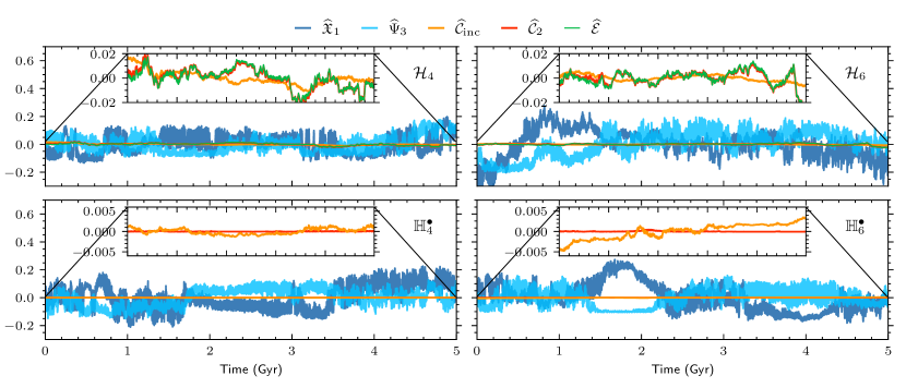
Figure 2: Time evolution over 5 Gyr of the dimensionless QIs ($\widehat{\mathcal{C}}_{\textnormal{\scriptsize inc}},\widehat{\mathcal{C}}_{2},\widehat{\mathcal{E}}$) and of two representatives of the dimensionless action variables ($\widehat{\mathfrak{X}}_{1},\widehat{\Psi}_{3}$) along the nominal orbital solutions of different models. Top row: $\mathcal{H}_{4}$ and $\mathcal{H}_{6}$ ($\widehat{\mathcal{E}}$ stands for $\widehat{\mathcal{E}}_{4}$ and $\widehat{\mathcal{E}}_{6}$, respectively). Bottom row: $\mathbb{H}_{4}^{\bullet}$ and $\mathbb{H}_{6}^{\bullet}$ from Eq. (24) ($\widehat{\mathcal{E}}_{2n}^{\bullet}$ is exactly conserved and not shown). The time series are low-pass filtered with a cutoff frequency of 1 Myr^-1 and the mean over 5 Gyr is subtracted. The variations of the QIs are enlarged in the insets. The $\mathbb{H}_{2n}^{\bullet}$ models are introduced and discussed in Sec. IV.4.

IV.2 Slow variables

The QIs of motion $\mathcal{E}_{2n},\mathcal{C}_{\textnormal{\scriptsize inc}},\mathcal{C}_{2}$ are clearly strong candidates for slow variables once evaluated along the orbital solutions. In what follows, to assess the slowness of a dynamical quantity when compared to the typical variations of the action variables, we consider the variance of its time series along a numerical solution.

We define the dimensionless QIs

$$\widehat{\mathcal{C}}_{\textnormal{\scriptsize inc}}=\frac{\mathcal{C}_{\textnormal{\scriptsize inc}}}{\|\bm{\gamma}_{1}\|\textrm{C}_{0}},\quad\widehat{\mathcal{C}}_{2}=\frac{\mathcal{C}_{2}}{\|\bm{\gamma}_{2}\|\textrm{C}_{0}},\quad\widehat{\mathcal{E}}_{2n}=\frac{\mathcal{E}_{2n}}{\|\bm{\gamma}_{3}\|\textrm{C}_{0}},$$ (21)

where $\textrm{C}_{0}$ stands for the current total AMD of the inner planets, that is, the value of $\mathcal{C}_{\textnormal{\scriptsize ecc}}+\mathcal{C}_{\textnormal{\scriptsize inc}}$ at time zero. We stress that, by introducing the unit vectors $\widehat{\bm{\gamma}}_{i}=\bm{\gamma}_{i}/\|\bm{\gamma}_{i}\|$ for $i\in\{1,2,3\}$, one has $\widehat{\mathcal{C}}_{\textnormal{\scriptsize inc}}=C_{\widehat{\bm{\gamma}}_{1}}/\textrm{C}_{0}$ and $\widehat{\mathcal{C}}_{2}=C_{\widehat{\bm{\gamma}}_{2}}/\textrm{C}_{0}$. At degree 2, one also has $\widehat{\mathcal{E}}_{2}=C_{\widehat{\bm{\gamma}}_{3}}/\textrm{C}_{0}$. We then consider the ensembles of numerical integrations of $\mathcal{H}_{4}$ and $\mathcal{H}_{6}$, with very close initial conditions and spanning 100 Gyr in the future, that have been presented in Ref. [7]. The top row of Fig. 2 shows the time evolution over 5 Gyr of the dimensionless QIs and of two components of the dimensionless action vector $\widehat{\bm{I}}=\bm{I}/\textrm{C}_{0}$ along the nominal orbital solutions of the two ensembles. We subtract from each time series its mean over the plotted time span. The time series are low-pass filtered by employing the Kolmogorov-Zurbenko (KZ) filter with three iterations of the moving average [48, 4]. A cutoff frequency of 1 Myr^-1 is chosen to highlight the long-term diffusion that can be hidden by short-time quasi-periodic oscillations. This is in line with our definition of quasi-integrals based on contribution from resonant harmonics only. Figure 2 clearly shows that the QIs are slowly-diffusing variables when compared to an arbitrary function of the action variables. The behavior of the QIs along the nominal orbital solutions of Fig. 2 is confirmed by a statistical analysis in Appendix C. Figure 10 shows the time evolution of the distributions of the same quantities as Fig. 2 over the stable orbital solutions of the entire ensembles of 1080 numerical integrations of Ref. [7]. Figure 11 details the growth of the QI dispersion over time.

We remark that $\mathcal{C}_{2}$ and $\mathcal{E}_{2n}$ show very similar time evolutions along stable orbital solutions, as can be seen in the top row Fig. 2. This is explained by the interesting observation that the components of the unit vectors $\widehat{\bm{\gamma}}_{2}$ and $\widehat{\bm{\gamma}}_{3}$ differ from each other by only a few percent, as shown in Appendix B. However, we stress that the two vectors are in fact linearly independent: $\mathcal{C}_{2}$ does not depend on the actions $\mathfrak{X}_{1}$ and $\mathfrak{X}_{2}$, while $\mathcal{E}_{2n}$ does. The two QIs move away from each other when high eccentricities of Mercury are reached, that is, for large excursions of the Mercury-dominated action $\mathfrak{X}_{1}$.

IV.3 Weak resonances and Lyapunov spectrum

A fundamental result from Table III is that the symmetries introduced in Sect. IV.1 are still preserved by resonances that have half-widths an order of magnitude smaller than those of the strongest terms. It is natural to extract from ranking $\mathcal{R}_{1}$ the weak resonances that break the three symmetries. A new ranking of resonances $\mathcal{R}_{2}$ is defined in this way. Table IV.3 reports the 10 strongest symmetry-breaking resonances that change $\mathcal{E}_{2n},\mathcal{C}_{\textnormal{\scriptsize inc}},\mathcal{C}_{2}$, respectively. As in Table III, only harmonics that are resonant for more than 1% of the 5-Gyr time span of the nominal solution of Gauss’s dynamics are shown. The leading symmetry-breaking resonances have half-widths of about 0.01${}^{\prime\prime}\,{\textrm{yr}}^{-1}$. For each QI, the dominant contribution comes from harmonics involving Fourier modes of the outer planet forcing other than $g_{5}$: the Saturn-dominated modes $g_{6},s_{6}$ and the modes $g_{7},s_{7}$ mainly associated to Uranus. In the case of $\mathcal{C}_{\textnormal{\scriptsize inc}}$, there is also a contribution that starts at about 0.006${}^{\prime\prime}\,{\textrm{yr}}^{-1}$ with $\mathcal{F}_{8}=4g_{1}-g_{2}-g_{3}-s_{1}-2s_{2}+s_{4}$ and comes from high-order internal resonances, that is, resonances that involve only the d.o.f. of the inner planets. We remark that the decrease of the resonance half-width with the index of the harmonic in Table IV.3 is steeper for $\mathcal{C}_{\textnormal{\scriptsize inc}}$ than for $\mathcal{E}_{2n},\mathcal{C}_{2}$, and is accompanied by a greater presence of high-order resonances. This may notably explain why the secular variations of $\mathcal{C}_{\textnormal{\scriptsize inc}}$ are somewhat smaller in the top row of Fig. 2. We finally point out the important symmetry-breaking role of the modes $g_{7},s_{7}$, representing the forcing mainly exerted by Uranus. Differently from what one might suppose, these modes cannot be completely neglected when addressing the long-term diffusion of ISS. This recalls the role of the modes $s_{7}$ and $s_{8}$ in the spin dynamics of Venus [49], and is basically a manifestation of the long-range nature of the gravitational interaction.

Table 3: Top of ranking $\mathcal{R}_{2}$. First 10 symmetry-breaking resonances of $\mathbb{H}_{10}$ along the 5-Gyr nominal solution of Gauss’s dynamics, that change $\mathcal{E}_{2n}$, $\mathcal{C}_{\textnormal{\scriptsize inc}}$, and $\mathcal{C}_{2}$, respectively (see Table III for details).

$1$ $g_{1}+g_{2}-2g_{5}+s_{2}-s_{7}$ $6$ 1% ${0.018}_{\mathchoice{\raisebox{2.0pt}{$\displaystyle\scriptscriptstyle 0.016$}}{\raisebox{2.0pt}{$\textstyle\scriptscriptstyle 0.016$}}{\raisebox{2.0pt}{$\scriptstyle\scriptscriptstyle 0.016$}}{\raisebox{2.0pt}{$\scriptscriptstyle\scriptscriptstyle 0.016$}}}^{\mathchoice{\raisebox{0.5pt}{$\displaystyle\scriptscriptstyle 0.020$}}{\raisebox{0.5pt}{$\textstyle\scriptscriptstyle 0.020$}}{\raisebox{0.5pt}{$\scriptstyle\scriptscriptstyle 0.020$}}{\raisebox{0.5pt}{$\scriptscriptstyle\scriptscriptstyle 0.020$}}}$ $2$ $g_{1}-2g_{2}+g_{6}-s_{2}+s_{6}$ $6$ 4% ${0.017}_{\mathchoice{\raisebox{2.0pt}{$\displaystyle\scriptscriptstyle 0.008$}}{\raisebox{2.0pt}{$\textstyle\scriptscriptstyle 0.008$}}{\raisebox{2.0pt}{$\scriptstyle\scriptscriptstyle 0.008$}}{\raisebox{2.0pt}{$\scriptscriptstyle\scriptscriptstyle 0.008$}}}^{\mathchoice{\raisebox{0.5pt}{$\displaystyle\scriptscriptstyle 0.024$}}{\raisebox{0.5pt}{$\textstyle\scriptscriptstyle 0.024$}}{\raisebox{0.5pt}{$\scriptstyle\scriptscriptstyle 0.024$}}{\raisebox{0.5pt}{$\scriptscriptstyle\scriptscriptstyle 0.024$}}}$ $3$ $g_{2}-g_{6}+s_{1}-s_{6}$ $4$ 8% ${0.011}_{\mathchoice{\raisebox{2.0pt}{$\displaystyle\scriptscriptstyle 0.003$}}{\raisebox{2.0pt}{$\textstyle\scriptscriptstyle 0.003$}}{\raisebox{2.0pt}{$\scriptstyle\scriptscriptstyle 0.003$}}{\raisebox{2.0pt}{$\scriptscriptstyle\scriptscriptstyle 0.003$}}}^{\mathchoice{\raisebox{0.5pt}{$\displaystyle\scriptscriptstyle 0.017$}}{\raisebox{0.5pt}{$\textstyle\scriptscriptstyle 0.017$}}{\raisebox{0.5pt}{$\scriptstyle\scriptscriptstyle 0.017$}}{\raisebox{0.5pt}{$\scriptscriptstyle\scriptscriptstyle 0.017$}}}$ $4$ $g_{4}-g_{6}-2s_{3}+3s_{4}-s_{6}$ $8$ 5% ${0.010}_{\mathchoice{\raisebox{2.0pt}{$\displaystyle\scriptscriptstyle 0.002$}}{\raisebox{2.0pt}{$\textstyle\scriptscriptstyle 0.002$}}{\raisebox{2.0pt}{$\scriptstyle\scriptscriptstyle 0.002$}}{\raisebox{2.0pt}{$\scriptscriptstyle\scriptscriptstyle 0.002$}}}^{\mathchoice{\raisebox{0.5pt}{$\displaystyle\scriptscriptstyle 0.012$}}{\raisebox{0.5pt}{$\textstyle\scriptscriptstyle 0.012$}}{\raisebox{0.5pt}{$\scriptstyle\scriptscriptstyle 0.012$}}{\raisebox{0.5pt}{$\scriptscriptstyle\scriptscriptstyle 0.012$}}}$ $5$ $2g_{1}-2g_{5}+s_{1}-s_{7}$ $6$ 1% ${0.007}_{\mathchoice{\raisebox{2.0pt}{$\displaystyle\scriptscriptstyle 0.005$}}{\raisebox{2.0pt}{$\textstyle\scriptscriptstyle 0.005$}}{\raisebox{2.0pt}{$\scriptstyle\scriptscriptstyle 0.005$}}{\raisebox{2.0pt}{$\scriptscriptstyle\scriptscriptstyle 0.005$}}}^{\mathchoice{\raisebox{0.5pt}{$\displaystyle\scriptscriptstyle 0.008$}}{\raisebox{0.5pt}{$\textstyle\scriptscriptstyle 0.008$}}{\raisebox{0.5pt}{$\scriptstyle\scriptscriptstyle 0.008$}}{\raisebox{0.5pt}{$\scriptscriptstyle\scriptscriptstyle 0.008$}}}$ $6$ $4g_{1}-3g_{2}-g_{5}-s_{2}+s_{7}$ $10$ 7% ${0.006}_{\mathchoice{\raisebox{2.0pt}{$\displaystyle\scriptscriptstyle 0.003$}}{\raisebox{2.0pt}{$\textstyle\scriptscriptstyle 0.003$}}{\raisebox{2.0pt}{$\scriptstyle\scriptscriptstyle 0.003$}}{\raisebox{2.0pt}{$\scriptscriptstyle\scriptscriptstyle 0.003$}}}^{\mathchoice{\raisebox{0.5pt}{$\displaystyle\scriptscriptstyle 0.015$}}{\raisebox{0.5pt}{$\textstyle\scriptscriptstyle 0.015$}}{\raisebox{0.5pt}{$\scriptstyle\scriptscriptstyle 0.015$}}{\raisebox{0.5pt}{$\scriptscriptstyle\scriptscriptstyle 0.015$}}}$ $7$ $g_{3}-g_{6}-2s_{3}+3s_{4}-s_{6}$ $8$ 2% ${0.006}_{\mathchoice{\raisebox{2.0pt}{$\displaystyle\scriptscriptstyle 0.003$}}{\raisebox{2.0pt}{$\textstyle\scriptscriptstyle 0.003$}}{\raisebox{2.0pt}{$\scriptstyle\scriptscriptstyle 0.003$}}{\raisebox{2.0pt}{$\scriptscriptstyle\scriptscriptstyle 0.003$}}}^{\mathchoice{\raisebox{0.5pt}{$\displaystyle\scriptscriptstyle 0.011$}}{\raisebox{0.5pt}{$\textstyle\scriptscriptstyle 0.011$}}{\raisebox{0.5pt}{$\scriptstyle\scriptscriptstyle 0.011$}}{\raisebox{0.5pt}{$\scriptscriptstyle\scriptscriptstyle 0.011$}}}$ $8$ $4g_{1}-g_{2}-g_{3}-s_{1}-2s_{2}+s_{4}$ $10$ 2% ${0.006}_{\mathchoice{\raisebox{2.0pt}{$\displaystyle\scriptscriptstyle 0.001$}}{\raisebox{2.0pt}{$\textstyle\scriptscriptstyle 0.001$}}{\raisebox{2.0pt}{$\scriptstyle\scriptscriptstyle 0.001$}}{\raisebox{2.0pt}{$\scriptscriptstyle\scriptscriptstyle 0.001$}}}^{\mathchoice{\raisebox{0.5pt}{$\displaystyle\scriptscriptstyle 0.009$}}{\raisebox{0.5pt}{$\textstyle\scriptscriptstyle 0.009$}}{\raisebox{0.5pt}{$\scriptstyle\scriptscriptstyle 0.009$}}{\raisebox{0.5pt}{$\scriptscriptstyle\scriptscriptstyle 0.009$}}}$ $9$ $2g_{1}-g_{2}-g_{5}+3s_{1}-2s_{2}-s_{7}$ $10$ 3% ${0.006}_{\mathchoice{\raisebox{2.0pt}{$\displaystyle\scriptscriptstyle 0.002$}}{\raisebox{2.0pt}{$\textstyle\scriptscriptstyle 0.002$}}{\raisebox{2.0pt}{$\scriptstyle\scriptscriptstyle 0.002$}}{\raisebox{2.0pt}{$\scriptscriptstyle\scriptscriptstyle 0.002$}}}^{\mathchoice{\raisebox{0.5pt}{$\displaystyle\scriptscriptstyle 0.008$}}{\raisebox{0.5pt}{$\textstyle\scriptscriptstyle 0.008$}}{\raisebox{0.5pt}{$\scriptstyle\scriptscriptstyle 0.008$}}{\raisebox{0.5pt}{$\scriptscriptstyle\scriptscriptstyle 0.008$}}}$ $10$ $3g_{1}-3g_{2}+s_{1}-2s_{2}+s_{7}$ $10$ 19% ${0.006}_{\mathchoice{\raisebox{2.0pt}{$\displaystyle\scriptscriptstyle 0.002$}}{\raisebox{2.0pt}{$\textstyle\scriptscriptstyle 0.002$}}{\raisebox{2.0pt}{$\scriptstyle\scriptscriptstyle 0.002$}}{\raisebox{2.0pt}{$\scriptscriptstyle\scriptscriptstyle 0.002$}}}^{\mathchoice{\raisebox{0.5pt}{$\displaystyle\scriptscriptstyle 0.009$}}{\raisebox{0.5pt}{$\textstyle\scriptscriptstyle 0.009$}}{\raisebox{0.5pt}{$\scriptstyle\scriptscriptstyle 0.009$}}{\raisebox{0.5pt}{$\scriptscriptstyle\scriptscriptstyle 0.009$}}}$    $\mathcal{C}_{2}$    $1$ $g_{1}+g_{2}-2g_{5}+s_{2}-s_{7}$ $6$ 1% ${0.018}_{\mathchoice{\raisebox{2.0pt}{$\displaystyle\scriptscriptstyle 0.016$}}{\raisebox{2.0pt}{$\textstyle\scriptscriptstyle 0.016$}}{\raisebox{2.0pt}{$\scriptstyle\scriptscriptstyle 0.016$}}{\raisebox{2.0pt}{$\scriptscriptstyle\scriptscriptstyle 0.016$}}}^{\mathchoice{\raisebox{0.5pt}{$\displaystyle\scriptscriptstyle 0.020$}}{\raisebox{0.5pt}{$\textstyle\scriptscriptstyle 0.020$}}{\raisebox{0.5pt}{$\scriptstyle\scriptscriptstyle 0.020$}}{\raisebox{0.5pt}{$\scriptscriptstyle\scriptscriptstyle 0.020$}}}$ $2$ $g_{1}-2g_{2}+g_{6}-s_{2}+s_{6}$ $6$ 4% ${0.017}_{\mathchoice{\raisebox{2.0pt}{$\displaystyle\scriptscriptstyle 0.008$}}{\raisebox{2.0pt}{$\textstyle\scriptscriptstyle 0.008$}}{\raisebox{2.0pt}{$\scriptstyle\scriptscriptstyle 0.008$}}{\raisebox{2.0pt}{$\scriptscriptstyle\scriptscriptstyle 0.008$}}}^{\mathchoice{\raisebox{0.5pt}{$\displaystyle\scriptscriptstyle 0.024$}}{\raisebox{0.5pt}{$\textstyle\scriptscriptstyle 0.024$}}{\raisebox{0.5pt}{$\scriptstyle\scriptscriptstyle 0.024$}}{\raisebox{0.5pt}{$\scriptscriptstyle\scriptscriptstyle 0.024$}}}$ $3$ $g_{3}-g_{6}+s_{2}-s_{4}$ $4$ 10% ${0.017}_{\mathchoice{\raisebox{2.0pt}{$\displaystyle\scriptscriptstyle 0.009$}}{\raisebox{2.0pt}{$\textstyle\scriptscriptstyle 0.009$}}{\raisebox{2.0pt}{$\scriptstyle\scriptscriptstyle 0.009$}}{\raisebox{2.0pt}{$\scriptscriptstyle\scriptscriptstyle 0.009$}}}^{\mathchoice{\raisebox{0.5pt}{$\displaystyle\scriptscriptstyle 0.022$}}{\raisebox{0.5pt}{$\textstyle\scriptscriptstyle 0.022$}}{\raisebox{0.5pt}{$\scriptstyle\scriptscriptstyle 0.022$}}{\raisebox{0.5pt}{$\scriptscriptstyle\scriptscriptstyle 0.022$}}}$ $4$ $g_{4}-g_{6}+s_{2}-s_{4}$ $4$ 4% ${0.016}_{\mathchoice{\raisebox{2.0pt}{$\displaystyle\scriptscriptstyle 0.007$}}{\raisebox{2.0pt}{$\textstyle\scriptscriptstyle 0.007$}}{\raisebox{2.0pt}{$\scriptstyle\scriptscriptstyle 0.007$}}{\raisebox{2.0pt}{$\scriptscriptstyle\scriptscriptstyle 0.007$}}}^{\mathchoice{\raisebox{0.5pt}{$\displaystyle\scriptscriptstyle 0.021$}}{\raisebox{0.5pt}{$\textstyle\scriptscriptstyle 0.021$}}{\raisebox{0.5pt}{$\scriptstyle\scriptscriptstyle 0.021$}}{\raisebox{0.5pt}{$\scriptscriptstyle\scriptscriptstyle 0.021$}}}$ $5$ $g_{2}-2g_{4}+g_{6}$ $4$ 12% ${0.016}_{\mathchoice{\raisebox{2.0pt}{$\displaystyle\scriptscriptstyle 0.009$}}{\raisebox{2.0pt}{$\textstyle\scriptscriptstyle 0.009$}}{\raisebox{2.0pt}{$\scriptstyle\scriptscriptstyle 0.009$}}{\raisebox{2.0pt}{$\scriptscriptstyle\scriptscriptstyle 0.009$}}}^{\mathchoice{\raisebox{0.5pt}{$\displaystyle\scriptscriptstyle 0.027$}}{\raisebox{0.5pt}{$\textstyle\scriptscriptstyle 0.027$}}{\raisebox{0.5pt}{$\scriptstyle\scriptscriptstyle 0.027$}}{\raisebox{0.5pt}{$\scriptscriptstyle\scriptscriptstyle 0.027$}}}$ $6$ $g_{1}-g_{3}-g_{5}+g_{6}-s_{1}+s_{4}$ $6$ 6% ${0.015}_{\mathchoice{\raisebox{2.0pt}{$\displaystyle\scriptscriptstyle 0.011$}}{\raisebox{2.0pt}{$\textstyle\scriptscriptstyle 0.011$}}{\raisebox{2.0pt}{$\scriptstyle\scriptscriptstyle 0.011$}}{\raisebox{2.0pt}{$\scriptscriptstyle\scriptscriptstyle 0.011$}}}^{\mathchoice{\raisebox{0.5pt}{$\displaystyle\scriptscriptstyle 0.024$}}{\raisebox{0.5pt}{$\textstyle\scriptscriptstyle 0.024$}}{\raisebox{0.5pt}{$\scriptstyle\scriptscriptstyle 0.024$}}{\raisebox{0.5pt}{$\scriptscriptstyle\scriptscriptstyle 0.024$}}}$ $7$ $g_{2}+g_{3}-3g_{4}+g_{6}$ $6$ 3% ${0.014}_{\mathchoice{\raisebox{2.0pt}{$\displaystyle\scriptscriptstyle 0.010$}}{\raisebox{2.0pt}{$\textstyle\scriptscriptstyle 0.010$}}{\raisebox{2.0pt}{$\scriptstyle\scriptscriptstyle 0.010$}}{\raisebox{2.0pt}{$\scriptscriptstyle\scriptscriptstyle 0.010$}}}^{\mathchoice{\raisebox{0.5pt}{$\displaystyle\scriptscriptstyle 0.017$}}{\raisebox{0.5pt}{$\textstyle\scriptscriptstyle 0.017$}}{\raisebox{0.5pt}{$\scriptstyle\scriptscriptstyle 0.017$}}{\raisebox{0.5pt}{$\scriptscriptstyle\scriptscriptstyle 0.017$}}}$ $8$ $g_{2}-2g_{3}+g_{6}+s_{3}-s_{4}$ $6$ 3% ${0.011}_{\mathchoice{\raisebox{2.0pt}{$\displaystyle\scriptscriptstyle 0.003$}}{\raisebox{2.0pt}{$\textstyle\scriptscriptstyle 0.003$}}{\raisebox{2.0pt}{$\scriptstyle\scriptscriptstyle 0.003$}}{\raisebox{2.0pt}{$\scriptscriptstyle\scriptscriptstyle 0.003$}}}^{\mathchoice{\raisebox{0.5pt}{$\displaystyle\scriptscriptstyle 0.018$}}{\raisebox{0.5pt}{$\textstyle\scriptscriptstyle 0.018$}}{\raisebox{0.5pt}{$\scriptstyle\scriptscriptstyle 0.018$}}{\raisebox{0.5pt}{$\scriptscriptstyle\scriptscriptstyle 0.018$}}}$ $9$ $g_{1}-g_{3}-g_{4}+g_{6}+s_{1}-s_{2}$ $6$ 4% ${0.011}_{\mathchoice{\raisebox{2.0pt}{$\displaystyle\scriptscriptstyle 0.008$}}{\raisebox{2.0pt}{$\textstyle\scriptscriptstyle 0.008$}}{\raisebox{2.0pt}{$\scriptstyle\scriptscriptstyle 0.008$}}{\raisebox{2.0pt}{$\scriptscriptstyle\scriptscriptstyle 0.008$}}}^{\mathchoice{\raisebox{0.5pt}{$\displaystyle\scriptscriptstyle 0.013$}}{\raisebox{0.5pt}{$\textstyle\scriptscriptstyle 0.013$}}{\raisebox{0.5pt}{$\scriptstyle\scriptscriptstyle 0.013$}}{\raisebox{0.5pt}{$\scriptscriptstyle\scriptscriptstyle 0.013$}}}$ $10$ $g_{2}-g_{6}+s_{1}-s_{6}$ $4$ 8% ${0.011}_{\mathchoice{\raisebox{2.0pt}{$\displaystyle\scriptscriptstyle 0.003$}}{\raisebox{2.0pt}{$\textstyle\scriptscriptstyle 0.003$}}{\raisebox{2.0pt}{$\scriptstyle\scriptscriptstyle 0.003$}}{\raisebox{2.0pt}{$\scriptscriptstyle\scriptscriptstyle 0.003$}}}^{\mathchoice{\raisebox{0.5pt}{$\displaystyle\scriptscriptstyle 0.017$}}{\raisebox{0.5pt}{$\textstyle\scriptscriptstyle 0.017$}}{\raisebox{0.5pt}{$\scriptstyle\scriptscriptstyle 0.017$}}{\raisebox{0.5pt}{$\scriptscriptstyle\scriptscriptstyle 0.017$}}}$

Table 4: Top of ranking $\mathcal{R}_{3}$. First 10 symmetry-breaking resonances of $\mathbb{H}_{10}$ along the 5-Gyr nominal solution of Gauss’s dynamics, that only involve $g_{5}$ among the external modes and change $\mathcal{E}_{2n}$, $\mathcal{C}_{\textnormal{\scriptsize inc}}$, and $\mathcal{C}_{2}$, respectively.

$1$ $g_{1}-3g_{2}+2g_{5}-s_{1}+2s_{2}-s_{4}$ $10$ 0.01‰ ${$110-04$}_{\mathchoice{\raisebox{2.0pt}{$\displaystyle\scriptscriptstyle$110-04$$}}{\raisebox{2.0pt}{$\textstyle\scriptscriptstyle$110-04$$}}{\raisebox{2.0pt}{$\scriptstyle\scriptscriptstyle$110-04$$}}{\raisebox{2.0pt}{$\scriptscriptstyle\scriptscriptstyle$110-04$$}}}^{\mathchoice{\raisebox{0.5pt}{$\displaystyle\scriptscriptstyle$110-04$$}}{\raisebox{0.5pt}{$\textstyle\scriptscriptstyle$110-04$$}}{\raisebox{0.5pt}{$\scriptstyle\scriptscriptstyle$110-04$$}}{\raisebox{0.5pt}{$\scriptscriptstyle\scriptscriptstyle$110-04$$}}}$ $2$ $2g_{1}-4g_{2}+2g_{5}+s_{2}-s_{4}$ $10$ 0.08‰ ${$810-05$}_{\mathchoice{\raisebox{2.0pt}{$\displaystyle\scriptscriptstyle$210-05$$}}{\raisebox{2.0pt}{$\textstyle\scriptscriptstyle$210-05$$}}{\raisebox{2.0pt}{$\scriptstyle\scriptscriptstyle$210-05$$}}{\raisebox{2.0pt}{$\scriptscriptstyle\scriptscriptstyle$210-05$$}}}^{\mathchoice{\raisebox{0.5pt}{$\displaystyle\scriptscriptstyle$110-04$$}}{\raisebox{0.5pt}{$\textstyle\scriptscriptstyle$110-04$$}}{\raisebox{0.5pt}{$\scriptstyle\scriptscriptstyle$110-04$$}}{\raisebox{0.5pt}{$\scriptscriptstyle\scriptscriptstyle$110-04$$}}}$ $3$ $3g_{2}-3g_{5}+s_{1}-2s_{2}+s_{3}$ $10$ 0.01‰ ${$310-05$}_{\mathchoice{\raisebox{2.0pt}{$\displaystyle\scriptscriptstyle$310-05$$}}{\raisebox{2.0pt}{$\textstyle\scriptscriptstyle$310-05$$}}{\raisebox{2.0pt}{$\scriptstyle\scriptscriptstyle$310-05$$}}{\raisebox{2.0pt}{$\scriptscriptstyle\scriptscriptstyle$310-05$$}}}^{\mathchoice{\raisebox{0.5pt}{$\displaystyle\scriptscriptstyle$310-05$$}}{\raisebox{0.5pt}{$\textstyle\scriptscriptstyle$310-05$$}}{\raisebox{0.5pt}{$\scriptstyle\scriptscriptstyle$310-05$$}}{\raisebox{0.5pt}{$\scriptscriptstyle\scriptscriptstyle$310-05$$}}}$ $4$ $g_{1}-4g_{2}+g_{3}+2g_{5}-s_{1}+s_{2}$ $10$ 0.13‰ ${$310-05$}_{\mathchoice{\raisebox{2.0pt}{$\displaystyle\scriptscriptstyle$210-06$$}}{\raisebox{2.0pt}{$\textstyle\scriptscriptstyle$210-06$$}}{\raisebox{2.0pt}{$\scriptstyle\scriptscriptstyle$210-06$$}}{\raisebox{2.0pt}{$\scriptscriptstyle\scriptscriptstyle$210-06$$}}}^{\mathchoice{\raisebox{0.5pt}{$\displaystyle\scriptscriptstyle$510-05$$}}{\raisebox{0.5pt}{$\textstyle\scriptscriptstyle$510-05$$}}{\raisebox{0.5pt}{$\scriptstyle\scriptscriptstyle$510-05$$}}{\raisebox{0.5pt}{$\scriptscriptstyle\scriptscriptstyle$510-05$$}}}$ $5$ $g_{1}+3g_{2}-4g_{5}-s_{2}+s_{4}$ $10$ 0.56‰ ${$310-05$}_{\mathchoice{\raisebox{2.0pt}{$\displaystyle\scriptscriptstyle$210-05$$}}{\raisebox{2.0pt}{$\textstyle\scriptscriptstyle$210-05$$}}{\raisebox{2.0pt}{$\scriptstyle\scriptscriptstyle$210-05$$}}{\raisebox{2.0pt}{$\scriptscriptstyle\scriptscriptstyle$210-05$$}}}^{\mathchoice{\raisebox{0.5pt}{$\displaystyle\scriptscriptstyle$410-05$$}}{\raisebox{0.5pt}{$\textstyle\scriptscriptstyle$410-05$$}}{\raisebox{0.5pt}{$\scriptstyle\scriptscriptstyle$410-05$$}}{\raisebox{0.5pt}{$\scriptscriptstyle\scriptscriptstyle$410-05$$}}}$ $6$ $g_{1}-4g_{2}+3g_{5}+s_{2}-s_{4}$ $10$ 0.01‰ ${$210-05$}_{\mathchoice{\raisebox{2.0pt}{$\displaystyle\scriptscriptstyle$210-05$$}}{\raisebox{2.0pt}{$\textstyle\scriptscriptstyle$210-05$$}}{\raisebox{2.0pt}{$\scriptstyle\scriptscriptstyle$210-05$$}}{\raisebox{2.0pt}{$\scriptscriptstyle\scriptscriptstyle$210-05$$}}}^{\mathchoice{\raisebox{0.5pt}{$\displaystyle\scriptscriptstyle$210-05$$}}{\raisebox{0.5pt}{$\textstyle\scriptscriptstyle$210-05$$}}{\raisebox{0.5pt}{$\scriptstyle\scriptscriptstyle$210-05$$}}{\raisebox{0.5pt}{$\scriptscriptstyle\scriptscriptstyle$210-05$$}}}$ $7$ $3g_{2}-3g_{5}+s_{1}-2s_{2}+s_{4}$ $10$ 0.13‰ ${$110-05$}_{\mathchoice{\raisebox{2.0pt}{$\displaystyle\scriptscriptstyle$710-06$$}}{\raisebox{2.0pt}{$\textstyle\scriptscriptstyle$710-06$$}}{\raisebox{2.0pt}{$\scriptstyle\scriptscriptstyle$710-06$$}}{\raisebox{2.0pt}{$\scriptscriptstyle\scriptscriptstyle$710-06$$}}}^{\mathchoice{\raisebox{0.5pt}{$\displaystyle\scriptscriptstyle$310-05$$}}{\raisebox{0.5pt}{$\textstyle\scriptscriptstyle$310-05$$}}{\raisebox{0.5pt}{$\scriptstyle\scriptscriptstyle$310-05$$}}{\raisebox{0.5pt}{$\scriptscriptstyle\scriptscriptstyle$310-05$$}}}$ $8$ $4g_{2}-g_{3}-g_{4}-2g_{5}+s_{1}-s_{3}$ $10$ 0.03‰ ${$110-05$}_{\mathchoice{\raisebox{2.0pt}{$\displaystyle\scriptscriptstyle$910-06$$}}{\raisebox{2.0pt}{$\textstyle\scriptscriptstyle$910-06$$}}{\raisebox{2.0pt}{$\scriptstyle\scriptscriptstyle$910-06$$}}{\raisebox{2.0pt}{$\scriptscriptstyle\scriptscriptstyle$910-06$$}}}^{\mathchoice{\raisebox{0.5pt}{$\displaystyle\scriptscriptstyle$110-05$$}}{\raisebox{0.5pt}{$\textstyle\scriptscriptstyle$110-05$$}}{\raisebox{0.5pt}{$\scriptstyle\scriptscriptstyle$110-05$$}}{\raisebox{0.5pt}{$\scriptscriptstyle\scriptscriptstyle$110-05$$}}}$ $9$ $2g_{1}-5g_{2}+g_{4}+2g_{5}$ $10$ 0.02‰ ${$910-06$}_{\mathchoice{\raisebox{2.0pt}{$\displaystyle\scriptscriptstyle$910-06$$}}{\raisebox{2.0pt}{$\textstyle\scriptscriptstyle$910-06$$}}{\raisebox{2.0pt}{$\scriptstyle\scriptscriptstyle$910-06$$}}{\raisebox{2.0pt}{$\scriptscriptstyle\scriptscriptstyle$910-06$$}}}^{\mathchoice{\raisebox{0.5pt}{$\displaystyle\scriptscriptstyle$910-06$$}}{\raisebox{0.5pt}{$\textstyle\scriptscriptstyle$910-06$$}}{\raisebox{0.5pt}{$\scriptstyle\scriptscriptstyle$910-06$$}}{\raisebox{0.5pt}{$\scriptscriptstyle\scriptscriptstyle$910-06$$}}}$ $10$ $2g_{1}-5g_{2}+g_{3}+2g_{5}$ $10$ 0.14‰ ${$610-06$}_{\mathchoice{\raisebox{2.0pt}{$\displaystyle\scriptscriptstyle$310-06$$}}{\raisebox{2.0pt}{$\textstyle\scriptscriptstyle$310-06$$}}{\raisebox{2.0pt}{$\scriptstyle\scriptscriptstyle$310-06$$}}{\raisebox{2.0pt}{$\scriptscriptstyle\scriptscriptstyle$310-06$$}}}^{\mathchoice{\raisebox{0.5pt}{$\displaystyle\scriptscriptstyle$810-06$$}}{\raisebox{0.5pt}{$\textstyle\scriptscriptstyle$810-06$$}}{\raisebox{0.5pt}{$\scriptstyle\scriptscriptstyle$810-06$$}}{\raisebox{0.5pt}{$\scriptscriptstyle\scriptscriptstyle$810-06$$}}}$

As we state in Sect. III, a pair of Lyapunov exponents would vanish if there were an exact integral of motion. In the presence of a weakly broken symmetry, one may expect a small positive Lyapunov exponent whose value relates to the half-width of the strongest resonances driving the time variation of the corresponding QI. Such an argument is a natural extension of the correspondence between the FT-MLE and the top of the resonance spectrum given in Eq. (12). Comparison of Table IV.3 with the Lyapunov spectrum in Fig. 1a shows that the time statistics of the half-widths of the symmetry-breaking resonances of ranking $\mathcal{R}_{2}$ overlaps with the ensemble distribution of the three smallest FT-LCEs, that is, $\lambda_{6},\lambda_{7},\lambda_{8}$. One can indeed write

$$2\pi\lambda_{6}\approx\Delta\omega^{\mathcal{R}_{2}},$$ (22)

where $\Delta\omega^{\mathcal{R}_{2}}$ stands for the half-width of the uppermost resonances of ranking $\mathcal{R}_{2}$. Table IV.3 and Fig. 1a suggest a relation between the QIs and the smallest Lyapunov exponents:

$$\lambda_{6},\lambda_{7},\lambda_{8}\longleftrightarrow\mathcal{E}_{2n},\mathcal{C}_{\textnormal{\scriptsize inc}},\mathcal{C}_{2}.$$ (23)

Equation (23) is not a one-to-one correspondence, nor should it be understood as an exact relation since, for example, $\lambda_{6}$ is not well separated from the larger exponents. Its physical meaning is that the QIs are among the slowest d.o.f. of the ISS dynamics. Such a claim is one of the core points of this work. In Sect. V, we show its statistical validity in the geometric framework established by a principal component analysis of the orbital solutions. Moreover, Sect. IV.4 shows that Eq. (23) can be stated more precisely in the case of a simplified dynamics that underlies $\mathbb{H}_{2n}$. We remark that $\mathcal{E}_{2n},\mathcal{C}_{\textnormal{\scriptsize inc}},\mathcal{C}_{2}$ constitute a set of three QIs that are independent and nearly in involution, and it is thus meaningful to associate three different Lyapunov exponents with them. On the one hand, the independence is easily checked at degree 2 as the vectors $\bm{\gamma}_{1},\bm{\gamma}_{2},\bm{\gamma}_{3}$ are linearly independent. On the other hand, one has the Poisson bracket $\{\mathcal{C}_{\textnormal{\scriptsize inc}},\mathcal{C}_{2}\}=0$, since the two quantities are functions of the action variables only. One also has $\{\mathcal{E}_{2n},\mathcal{C}_{\textnormal{\scriptsize inc}}\}=\{\mathbb{H}_{2n},\mathcal{C}_{\textnormal{\scriptsize inc}}\}=\dot{\mathcal{C}}_{\textnormal{\scriptsize inc}}$ and $\{\mathcal{E}_{2n},\mathcal{C}_{2}\}=\dot{\mathcal{C}}_{2}$. Only weak resonances contribute to these Poisson brackets and the three QIs are therefore nearly in involution.

IV.4 New truncation of the Hamiltonian

The fundamental role of the external modes $g_{6},g_{7},s_{6},s_{7}$ in Table IV.3 raises the question of which symmetry-breaking resonances persist if one excludes all the Fourier harmonics that involve external modes other than $g_{5}$. Therefore, we define a new ranking $\mathcal{R}_{3}$ by extracting such resonances from ranking $\mathcal{R}_{2}$. Table IV.3 reports the 10 strongest resonances per each broken symmetry. The difference with respect to Table IV.3 is manifest. As $g_{5}$ is the only external mode remaining, there are no resonances left that can contribute to the time evolution of $\mathcal{E}_{2n}$. For the remaining two QIs, the only harmonics that appear in Table IV.3 are of order 8 or higher, and this is accompanied by a significant drop in the half-width of the leading resonances. In the case of $\mathcal{C}_{\textnormal{\scriptsize inc}}$, the half-width of the uppermost resonances is now around 0.005${}^{\prime\prime}\,{\textrm{yr}}^{-1}$. One can appreciate that the activation times $\tau^{\mathrm{res}}$ of the resonances do not exceed a few percent, differently from Table IV.3. The most impressive change is, however, related to $\mathcal{C}_{2}$: only harmonics of order 10 appear in Table IV.3 and the half-width of the uppermost resonances drops by two orders of magnitude. We stress that such harmonics are resonant for very short periods of time along the 5 Gyr spanned by the nominal solution of Gauss’s dynamics. To retrieve the time statistics of the resonances affecting $\mathcal{C}_{2}$, we indeed choose to repeat the computations of Ref. [19] by increasing the cutoff frequency of the low-pass filter applied to time series of the action-angle variables from (5 Myr)^-1 to 1 Myr^-1 [19, Appendices F.2 and G.5]. The filtered time series have then been resampled with a timestep of 50 kyr. Many harmonics we show in Table IV.3 and related to $\mathcal{C}_{2}$ are resonant for a few timesteps and their time statistics is very tentative. More precise estimations of the half-widths should be obtained over an ensemble of different orbital solutions, possibly spanning more than 5 Gyr. In any case, the fundamental point here is the drastic reduction in the size of the uppermost resonances with respect to Table IV.3, and this is a robust result. We remark that resonances of order 12 and higher may also carry an important contribution at these scales, but they are excluded by the truncation at degree 10 adopted in Ref. [19] to establish the resonant harmonics, so they do not appear in the tables of this work.

Hamiltonian $\mathbb{H}_{2n}^{\bullet}$.

The implications of Table IV.3 suggest to introduce an additional truncation in the Hamiltonian $\mathbb{H}_{2n}$. This consists in dropping the harmonics of Eq. (6) that involve external modes other than $g_{5}$:

$$\mathbb{H}_{2n}^{\bullet}(\bm{I},\bm{\theta},t)=\sum_{\begin{subarray}{c}\bm{k},\ell_{1}\end{subarray}}\widetilde{\mathbb{H}}_{2n}^{\bm{k},\bm{\ell}^{\bullet}}\!(\bm{I})\mathrm{E}^{j\left(\bm{k}\cdot\bm{\theta}+\ell_{1}\phi_{1}(t)\right)},$$ (24)

where $\phi_{1}(t)=-g_{5}t$ and $\bm{\ell}^{\bullet}=(\ell_{1},0,\dots,0)$, with $\ell_{1}\in\mathbb{Z}$. Consistently with the absence of symmetry-breaking resonances related to $\mathcal{E}_{2n}$ in Table IV.3, the corresponding dynamics admits the exact integral of motion

$$\mathcal{E}_{2n}^{\bullet}=\mathbb{H}_{2n}^{\bullet}+g_{5}\textstyle{\sum_{i=1}^{4}}(\mathfrak{X}_{i}+\Psi_{i}),$$ (25)

which represents the transformed Hamiltonian under the canonical change of variables that eliminates the explicit time dependence in Eq. (24). We point out that, as the additional truncation is applied to the action-angle formulation of Eq. (6), the external modes other than $g_{5}$ still enter the definition of the proper modes of the forced Laplace-Lagrange dynamics [4]. The orbital solution arising from $\mathbb{H}_{2n}^{\bullet}$ is initially very close to that of $\mathbb{H}_{2n}$. A frequency analysis over the first 20 Myr shows that the differences in the fundamental frequencies of the motion between $\mathbb{H}_{2n}^{\bullet}$ and $\mathbb{H}_{2n}$ are of the order of $10^{-3}$ ${\textrm{arcsec yr}}^{-1}$, an order of magnitude smaller than the typical frequency differences between $\mathcal{H}_{4}$ and $\mathcal{H}_{6}$ [4, Table 3]. Therefore, even though $\mathbb{H}_{2n}^{\bullet}$ constitutes a simplification of $\mathbb{H}_{2n}$, it should not be regarded as a toy model. Its dynamics, in particular, still possesses 8 d.o.f.

We compute the Lyapunov spectrum of the Hamiltonian $\mathbb{H}_{4}^{\bullet}$ in the same way as described in Sect. III in the case of $\mathcal{H}_{2n}$. Since its dynamics turns out to be much more stable than that of $\mathcal{H}_{4}$ (see Sect. VI, Fig. 7), we extend the computation to a time span of 100 Gyr. The marginal ensemble PDFs of the positive FT-LCEs are shown in Fig 1b. Comparing to the Lyapunov spectrum of $\mathcal{H}_{4}$, one notices that the distributions of the leading exponents turn out to be quite similar, apart from being more spaced and except for a slight decrease in their median values. However, such a decrease is more pronounced for smaller exponents, and the drop in the smallest exponents is drastic. The smallest one, $\lambda_{8}$, decreases monotonically, consistently with the fact that $\mathcal{E}^{\bullet}_{4}$ from Eq. (25) is an exact integral of motion. The exponent $\lambda_{7}$ drops by more than an order of magnitude, and apparently begins to stabilize around a few $10^{-4}$ ${\textrm{arcsec yr}}^{-1}$, while $\lambda_{6}$ also reduces significantly, by a factor of three, to about 0.005${}^{\prime\prime}\,{\textrm{yr}}^{-1}$. The drop in the smallest exponents agrees remarkably well with that of the half-width of the leading symmetry-breaking resonances when switching from Table IV.3 to Table IV.3. One can indeed write

$$2\pi\lambda_{6} \approx\Delta\omega^{\mathcal{R}_{3},\mathcal{C}_{\textnormal{\scriptsize inc}}},$$ (26)

$$2\pi\lambda_{7} \approx\Delta\omega^{\mathcal{R}_{3},\mathcal{C}_{2}},$$

$$\lambda_{8} =0,$$

where $\Delta\omega^{\mathcal{R}_{3},Q}$ stands for the half-width of the uppermost resonances of ranking $\mathcal{R}_{3}$ related to the quasi-integral $Q$. The hierarchy of the three smallest exponents in the spectrum of Fig. 1b consistently follows that of the QIs suggested in Table IV.3 by the very different sizes of the leading resonances. In other words, one can state:

$$\lambda_{6} \longleftrightarrow\mathcal{C}_{\textnormal{\scriptsize inc}},$$ (27)

$$\lambda_{7} \longleftrightarrow\mathcal{C}_{2},$$

$$\lambda_{8} \longleftrightarrow\mathcal{E}_{2n}^{\bullet}.$$

These one-to-one correspondences are a particular case of Eq. (23) and support the physical intuition behind it. In Sect. V, we prove the validity of Eq. (27) in the geometric framework established by a principal component analysis of the orbital solutions of $\mathbb{H}_{2n}^{\bullet}$.

Numerical integrations.

We compute ensembles of 1080 orbital solutions of the dynamical models $\mathbb{H}_{4}^{\bullet}$ and $\mathbb{H}_{6}^{\bullet}$, with initial conditions very close to the nominal ones of Gauss’s dynamics and spanning 100 Gyr in the future. This closely follows what we did in Ref. [7] in the case of the models $\mathcal{H}_{2n}$. The bottom row of Fig. 2 shows the filtered dimensionless QIs along the nominal solutions of the two models over the first 5 Gyr. The hierarchy of the QIs stated in Eq. (27) is manifest. The quantity $\mathcal{C}_{2}$ has secular variations much slower than $\mathcal{C}_{\textnormal{\scriptsize inc}}$, while the latter is itself slower with respect to its counterpart in the orbital solutions of $\mathcal{H}_{2n}$. We remark that, as $\mathcal{E}_{2n}^{\bullet}$ is an exact integral of motion for the model $\mathbb{H}_{2n}^{\bullet}$, we do not plot it. From Fig. 2 it is also evident how difficult can be the retrieval of the short-lasting resonances affecting $\mathcal{C}_{2}$ from a solution of $\mathbb{H}_{2n}^{\bullet}$ spanning only a few billion years.

The hierarchy of the QIs is confirmed by a statistical analysis in Appendix C. Figure 10 shows the entire time evolution of the distributions of the filtered dimensionless QIs over the stable orbital solutions of the ensembles of 1080 numerical integrations. Figure 11 details the growth of the QI dispersion over time. As suggested by Table IV.3, the drop in the diffusion rates of the QIs when switching from $\mathcal{H}_{2n}$ to $\mathbb{H}_{2n}^{\bullet}$ is manifest.

V Statistical detection of slow variables

Section IV shows how the slow-fast nature of the ISS dynamics, indicated by the Lyapunov spectrum, emerges from the quasi-symmetries of the resonant harmonics of the Hamiltonian. QIs of motion can be introduced semi-analytically and they constitute slow quantities when evaluated along stable orbital solutions. In this section, we consider the slow variables that can be systematically retrieved from a numerically integrated orbital solution by means of a statistical technique, the principal component analysis. We show that, in the case of the forced secular ISS, the slowest variables are remarkably close to the QIs, and this can be established in a precise geometric framework.

V.1 Principal component analysis

PCA is a widely used classical technique for multivariate analysis [50, 51]. For a given dataset, PCA aims to find an orthogonal linear transformation of the variables such that the new coordinates offer a more condensed and representative view of the data. The new variables are called principal components (PCs). They are uncorrelated and ordered according to decreasing variance: the first PC and last one have, respectively, the largest and the smallest variance of any linear combination of the original variables. While one is typically interested in the PCs of largest variance, in this work we employ the variance of the time series of a dynamical quantity to assess its slowness when compared to the typical variations of the action variables (see Sect. IV.2). We thus perform a PCA of the action variables $\bm{I}$ and focus on the last PCs, as they give a pertinent statistical definition of slow variables. We stress that, when coupled to a low-pass filtering of the time series, the statistical variance provides a measure of chaotic diffusion.

Implementation.

Our procedure for the PCA is described briefly as follows [for general details see, e.g., 52, 53]. Let $\bm{I}(t)=(\bm{\mathfrak{X}}(t),\bm{\Psi}(t))$ be the 8-dimensional time series of the action variables evaluated along a numerical solution of the equations of motion. As in Sect. IV.2, we apply the KZ low-pass filter with three iterations of the moving average and a cutoff frequency of 1 Myr^-1 to obtain the filtered time series $\hat{\bm{I}}(t)$ [48, 4]. In this way, the short-term quasi-periodic oscillations are mostly suppressed, which better reveals the chaotic diffusion over longer timescales. We finally define the mean-subtracted filtered action variables over the time interval $[t_{0},t_{0}+T]$ as $\tilde{\bm{I}}(t)=\hat{\bm{I}}(t)-n^{-1}\sum_{i=0}^{n-1}\hat{\bm{I}}(t_{0}+i\Delta t)$, where the mean is estimated by discretization of the time series with a sampling step $\Delta t$ such that $T=(n-1)\Delta t$. The discretized time series over the given interval is stored in an $8\times n$ matrix:

$$\mathbf{D}=[\tilde{\bm{I}}(t_{0}),\ \tilde{\bm{I}}(t_{0}+\Delta t),\ \dots,\ \tilde{\bm{I}}(t_{0}+(n-1)\Delta t)].$$ (28)

The PCA of the data matrix $\mathbf{D}$ consists in a linear transformation $\mathbf{P}=\mathbf{A}^{\mathrm{T}}\mathbf{D}$, where $\mathbf{A}$ is an $8\times 8$ orthogonal matrix (i.e. $\mathbf{A}^{-1}=\mathbf{A}^{\mathrm{T}}$) defined as follows. By writing $\mathbf{A}=[\bm{a}_{1},\dots,\bm{a}_{8}]$, the column vectors $\bm{a}_{i}\in\mathbb{R}^{8}$ are chosen to be the normalized eigenvectors of the sample covariance matrix, in order of decreasing eigenvalues: $(n-1)^{-1}\mathbf{D}\mathbf{D}^{\mathrm{T}}=\mathbf{A}\bm{\Sigma}\mathbf{A}^{\mathrm{T}}$, where $\bm{\Sigma}=\text{diag}(\sigma_{1},\dots,\sigma_{8})$ and $\sigma_{1}\geq\dots\geq\sigma_{8}$. The PCs are defined as the new variables after the transformation, that is, $\text{PC}_{i}=\bm{a}_{i}\cdot\bm{I}$ with $i\in\{1,\dots,8\}$. The uncorrelatedness and the ordering of the PCs can be easily seen from the diagonal form of their sample covariance matrix, $(n-1)^{-1}\mathbf{P}\mathbf{P}^{\mathrm{T}}=\bm{\Sigma}$, from which it follows that the variance of $\text{PC}_{i}$ is $\sigma_{i}$.

Among all the linear combinations in the action variables $\bm{I}$, the last PC, i.e., $\text{PC}_{8}$, has the smallest variance over the time interval $[t_{0},t_{0}+T]$ of a given orbital solution. The second last PC, i.e., $\text{PC}_{7}$, has the second smallest variance and is uncorrelated with $\text{PC}_{8}$, and so on. It follows that the linear subspace spanned by the last $k$ PCs is the $k$-dimensional subspace of minimum variance: the variance of the sample projection onto this subspace is the minimum among all the subspaces of the same dimension. These properties indicate that the last PCs provide a pertinent statistical definition of slow variables along numerically integrated solutions of a dynamical system. The linear structure of the PCA, in particular, seems adapted to quasi-integrable systems close to a quadratic Hamiltonian, like the ISS. In such a case, one may reasonably expect that the slow variables are, to a first approximation, linear combinations of the action variables. We remark that the mutual orthogonality allows us to associate a linear d.o.f. to each PC.

Aggregated sample.

Instead of considering a specific solution, it is also possible to take the same time interval from $m$ different solutions, and stack them together to form an aggregated sample: $\mathbf{D}_{\mathrm{agg}}=[\mathbf{D}_{1},\mathbf{D}_{2},\dots,\mathbf{D}_{m}]$, where $\mathbf{D}_{i}$ is the data matrix of Eq. (28) for the $i$th solution. Since this work deals with a non-stationary dynamics, as the ISS ceaselessly diffuses in the phase space [7], we always consider the same time interval for each of the $m$ solutions. The aggregated sample is useful in capturing globally the behavior of the dynamics, because it averages out temporary and rare episodes arising along specific solutions.

V.2 Principal components and quasi-integrals

Both the QIs and the last PCs represent slow variables, but are established through two different methods. Equations (23) and (27) claim that the QIs found semi-analytically in Sect. IV are among the slowest d.o.f. of the ISS dynamics. This naturally suggests to compare the three QIs with the three last PCs retrieved from numerically integrated orbital solutions. In this part, we first introduce the procedure that we implement to establish a consistent and systematic correspondence between QIs and PCs. We then present both a visual and a quantitative geometric comparison between them.

V.2.1 Tweaking the QIs

The three last components PC₈, PC₇, PC₆ are represented by the set of vectors $S_{\mathrm{PCs}}=\{\bm{a}_{8},\bm{a}_{7},\bm{a}_{6}\}$ belonging to $\mathbb{R}^{8}$. By construction, these PCs have a linear, hierarchical, and orthogonal structure. In other words: the PCs are linear combinations of the action variables $\bm{I}$; denoting by $\preceq$ the order of statistical variance, one has $\mathrm{PC}_{8}\preceq\mathrm{PC}_{7}\preceq\mathrm{PC}_{6}$; the unit vectors $(\bm{a}_{i})_{i=6}^{8}$ are orthogonal to each other. On the other hand, the QIs of motion $\mathcal{C}_{\textnormal{\scriptsize inc}},\mathcal{C}_{2},\mathcal{E}_{2n}$ do not possess these properties. Therefore, we adjust them in such a way to reproduce the same structure.

Linearity.

While $\mathcal{C}_{\textnormal{\scriptsize inc}}$ and $\mathcal{C}_{2}$ are linear functions of the action variables, $\mathcal{E}_{2n}$ is not when $n>1$. Nevertheless, as we explain in Sect. IV.1, as far as one considers stable orbital solutions, the linear LL approximation $\mathcal{E}_{2}=\bm{\gamma}_{3}\cdot\bm{I}$ reproduces $\mathcal{E}_{2n}$ reasonably well. Therefore, we consider the three linear QIs of motion $\mathcal{C}_{\textnormal{\scriptsize inc}},\mathcal{C}_{2},\mathcal{E}_{2}$, which are respectively represented by the set of $\mathbb{R}^{8}$-vectors $S_{\mathrm{QIs}}=\{\bm{\gamma}_{1},\bm{\gamma}_{2},\bm{\gamma}_{3}\}$. In this way, the 3-dimensional linear subspaces of the action space spanned by the sets $S_{\mathrm{QIs}}$ and $S_{\mathrm{PCs}}$ can be compared.

Ordering.

We define a set of QIs that are ordered by statistical variance, as it is the case for the PCs. We follow two different approaches according to model $\mathbb{H}_{2n}^{\bullet}$ in Eq. (24) or $\mathbb{H}_{2n}$ in Eq. (6) (clearly $n>1$).

$\mathbb{H}_{2n}^{\bullet}$

A strong hierarchy of statistical variances among the QIs emerges from the size of the leading symmetry-breaking resonances in Table IV.3 and from the orbital solutions in Figs. 2, 10, and 11. One has $\mathcal{E}_{2n}^{\bullet}\prec\mathcal{C}_{2}\prec\mathcal{C}_{\textnormal{\scriptsize inc}}$. While $\mathcal{E}_{2n}^{\bullet}$ is an exact non-linear integral of motion, we expect that its linear truncation $\mathcal{E}_{2}^{\bullet}=\mathcal{E}_{2}$ varies more than $\mathcal{C}_{2}$ and $\mathcal{C}_{\textnormal{\scriptsize inc}}$. Therefore, we consider the ordered set of QIs of motion $\{\mathcal{C}_{2},\mathcal{C}_{\textnormal{\scriptsize inc}},\mathcal{E}_{2}\}$ represented by the ordered set of vectors $S^{\prime}_{\mathrm{QIs}}=\{\bm{\gamma}_{2},\bm{\gamma}_{1},\bm{\gamma}_{3}\}$.

$\mathbb{H}_{2n}$

Since the leading resonances affecting the QIs in Table IV.3 have comparable sizes, there is no clear order of statistical variances that can be inferred. We then implement a systematic approach that orders the QIs by simply inheriting the ordering of the PCs. More precisely, we define a set of ordered vectors $S_{\mathrm{QIs}}^{\prime}$ through the projections of the three last PCs onto the linear subspace generated by the QIs: $S_{\mathrm{QIs}}^{\prime}=\{\mathrm{proj}_{S_{\mathrm{QIs}}}(\bm{a}_{8}),\mathrm{proj}_{S_{\mathrm{QIs}}}(\bm{a}_{7}),\mathrm{proj}_{S_{\mathrm{QIs}}}(\bm{a}_{6})\}$. As a result, the new set of QIs mirrors the hierarchical structure of the PCs. We stress that $S_{\mathrm{QI}}^{\prime}$ spans the same subspace of $\mathbb{R}^{8}$ as $S_{\mathrm{QI}}$, since the ordered QIs are just linear combinations of the original ones.

Orthogonality.

We apply the Gram-Schmidt process to the ordered set $S_{\mathrm{QIs}}^{\prime}$ to obtain the orthonormal basis $S_{\mathrm{QIs}}^{\prime\prime}=\{\bm{\alpha}_{1},\bm{\alpha}_{2},\bm{\alpha}_{3}\}$. The set $S_{\mathrm{QIs}}^{\prime\prime}$ clearly spans the same subspace as $S_{\mathrm{QIs}}$. Moreover, the Gram-Schmidt process preserves the hierarchical structure, that is, the two $m$-dimensional subspaces spanned by the first $m\leq 3$ vectors of $S_{\mathrm{QIs}}^{\prime}$ and $S_{\mathrm{QIs}}^{\prime\prime}$, respectively, are identical.

In the end, we obtain a linear, ordered, and orthogonal set of modified QIs of motion $\{\mathrm{QI}_{1},\mathrm{QI}_{2},\mathrm{QI}_{3}\}$, where $\mathrm{QI}_{i}=\bm{\alpha}_{i}\cdot\bm{I}$.

V.2.2 Visual comparison

We now visually compare the vectors $\bm{\alpha}_{1,2,3}$ of the modified QIs with the corresponding vectors $\bm{a}_{8,7,6}$ of the last three PCs. We use the ensembles of 1080 numerically integrated orbital solutions of the models $\mathcal{H}_{4}$ and $\mathbb{H}_{4}$ considered in Sects. IV.2 and IV.4, respectively. The nominal solution of each set is denoted as sol. #1 from now on. For the model $\mathcal{H}_{4}$, we also consider two other solutions: sol. #2 that represents a typical evolution among the 1080 solutions, and sol. #3 representing a rarer one. The particular choice of these two solutions is detailed in Sect. V.2.3.

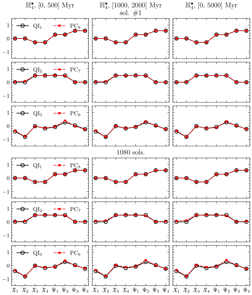
Figure 3: Vectors $\bm{\alpha}_{1,2,3}$ representing the three modified QIs (QI_1,2,3, black circles) compared to the corresponding vectors $\bm{a}_{8,7,6}$ of the three last PCs (PC_8,7,6, red dots), for the intervals [0, 500] Myr (left-hand column), [1000, 2000] Myr (middle column) and [0, 5000] Myr (right-hand column) of sol. #1 and of the aggregated sample of 1080 solutions of model $\mathbb{H}_{4}^{\bullet}$. Here, $\mathrm{QI}_{1}$ is proportional to $\mathcal{C}_{2}$ and $\mathrm{QI}_{2}$ is proportional to $\mathcal{C}_{2}^{\perp}$; see Eq. (20).

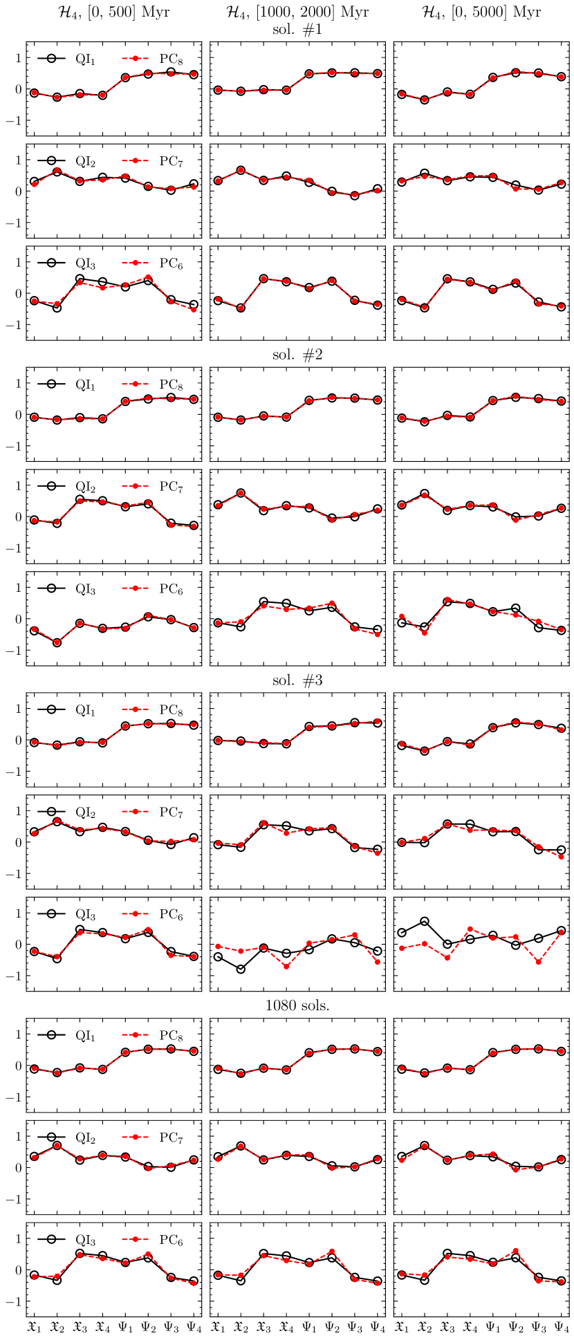
Figure 4: Vectors $\bm{\alpha}_{1,2,3}$ representing the three modified QIs (QI_1,2,3, black circles) compared to the corresponding vectors $\bm{a}_{8,7,6}$ of the three last PCs (PC_8,7,6, red dots), for the intervals [0, 500] Myr (left-hand column), [1000, 2000] Myr (middle column) and [0, 5000] Myr (right-hand column) of sol. #1, sol. #2, and sol. #3 and of the aggregated sample of 1080 solutions of model $\mathcal{H}_{4}$.

Hamiltonian $\mathbb{H}_{4}^{\bullet}$.

The modified QIs can be explicitly derived in this case and comprise interpretable physical quantities. One has $\mathrm{QI}_{1}$ proportional to $\mathcal{C}_{2}$ and $\mathrm{QI}_{2}$ proportional to $\mathcal{C}_{2}^{\perp}$. Moreover, $\mathrm{QI}_{3}$ is the component of $\mathcal{E}_{2}$ that is orthogonal to both $\mathcal{C}_{2}$ and $\mathcal{C}_{2}^{\perp}$. Figure 3 shows the comparison between the modified QIs and the corresponding PCs for three different time intervals along sol. #1 of $\mathbb{H}_{4}^{\bullet}$ (see Fig. 2 bottom left for its time evolution). The agreement of the pairs $(\mathrm{QI}_{1},\mathrm{PC}_{8})$, $(\mathrm{QI}_{2},\mathrm{PC}_{7})$, and $(\mathrm{QI}_{3},\mathrm{PC}_{6})$ across different intervals is manifest and even impressive. One can appreciate that the “slower” the PC, the more similar it is to its corresponding QI. The overlap between the modified QIs and the three last PCs means that the QIs of motion span the slowest 3-dimensional linear subspace of the action space. Therefore, to a linear approximation, they represent the three slowest d.o.f. of the $\mathbb{H}_{4}^{\bullet}$ dynamics. The quasi-integral $\mathcal{C}_{2}$ represents the slowest linear d.o.f.: it coincides with the last principal component PC₈, which has the smallest variance among all the linear combinations of the action variables. $\mathcal{C}_{\mathrm{inc}}$ and $\mathcal{E}_{2}$ represent the second and the third slowest linear d.o.f., respectively: the component of $\mathcal{C}_{\mathrm{inc}}$ orthogonal to $\mathcal{C}_{2}$, i.e., $\mathcal{C}_{2}^{\perp}$, matches the second last principal component PC₇; the component of $\mathcal{E}_{2}$ orthogonal to the subspace generated by ($\mathcal{C}_{2}$, $\mathcal{C}_{\mathrm{inc}}$) matches the third last principal component PC₆. The strong hierarchical structure of the slow variables for the simplified dynamics $\mathbb{H}_{4}^{\bullet}$ is clearly confirmed by the almost frozen basis vectors of the PCs.

Hamiltonian $\mathcal{H}_{4}$.

In this case, the QIs of motion $\mathcal{C}_{\textnormal{\scriptsize inc}},\mathcal{C}_{2},\mathcal{E}_{2}$ do not show a clear hierarchical structure in terms of statistical variance. Therefore, we consider the whole subspace spanned by the three QIs with respect to that spanned by the three last PCs. Since it is not easy to visually compare two 3-dimensional subspaces of $\mathbb{R}^{8}$, we compare their basis vectors instead. The basis $\bm{\alpha}_{1,2,3}$ of modified quasi-integrals QI_1,2,3 is computed according to the algorithm presented in Sect. V.2.1.

Figure 4 presents the comparison between the modified QIs and the corresponding PCs across three different time intervals of three solutions of $\mathcal{H}_{4}$ (see Fig. 5 for their time evolution). The first two, sols. #1 and #2, show thorough agreement between the pairs of QIs and PCs across all intervals, which indicates close proximity between the two subspaces $V_{\mathrm{QIs}}=\operatorname{span}(S_{\mathrm{QIs}})$ and $V_{\mathrm{PCs}}=\operatorname{span}(S_{\mathrm{PCs}})$. One can appreciate that the directions of the basis vectors are quite stable. The last component PC₈, in particular, remains close to $\mathcal{C}_{\textnormal{\scriptsize inc}}$. The slowest linear d.o.f. of $\mathcal{H}_{4}$ can thus be deduced to be close to $\mathcal{C}_{\textnormal{\scriptsize inc}}$, in line with the discussion in Sect. IV.3. Such a result shows how interesting physical insight can be gained through the PCA. Some changes in the basis vectors can arise, however, as for the first time interval of sol. #2. This may be expected from a dynamical point of view. Differently from $\mathbb{H}_{4}^{\bullet}$, there is no pronounced separation between the slowest d.o.f. at the bottom of the Lyapunov spectrum in Fig. 1a: the marginal distributions of consecutive exponents can indeed touch or overlap each other. Therefore, the hierarchy of slow variables is not as frozen as in $\mathbb{H}_{4}^{\bullet}$ and it can change along a given orbital solution.

Solutions #1 and #2 represent typical orbital evolutions. If the same time intervals of all the 1080 solutions are stacked together to form an aggregated sample on which the PCA is applied, the features mentioned above persist: the agreement between QIs and PCs, the stability of the basis vectors, and the similarity between PC₈ and $\mathcal{C}_{\mathrm{inc}}$ (see Fig. 4). Once again, the PCA confirms that the subspace spanned by the three QIs is overall close to the slowest 3-dimensional linear subspace of the action space. Therefore, to a linear approximation, they represent the three slowest d.o.f. of the $\mathcal{H}_{4}$ dynamics. We remark that the slowness of the 3-dimensional subspace spanned by the QIs is a much stronger constraint than the observation that each QI is a slow variable. To give an example, let $Q=\widehat{\bm{q}}\cdot\bm{I}$ be a slow variable with unit vector $\widehat{\bm{q}}$. If $\bm{\epsilon}$ is an arbitrary small vector, i.e. $\|\bm{\epsilon}\|\ll 1$, then $Q^{\prime}=(\widehat{\bm{q}}+\bm{\epsilon})\cdot\bm{I}$ can also be considered as a slow variable, whereas the normalized difference of two quantities, $\widehat{\bm{\epsilon}}\cdot\bm{I}$, is generally not. Therefore, the linear subspace spanned by $Q$ and $Q^{\prime}$, that is, by $\widehat{\bm{q}}$ and $\widehat{\bm{\epsilon}}$, is not a slow 2-dimensional subspace.

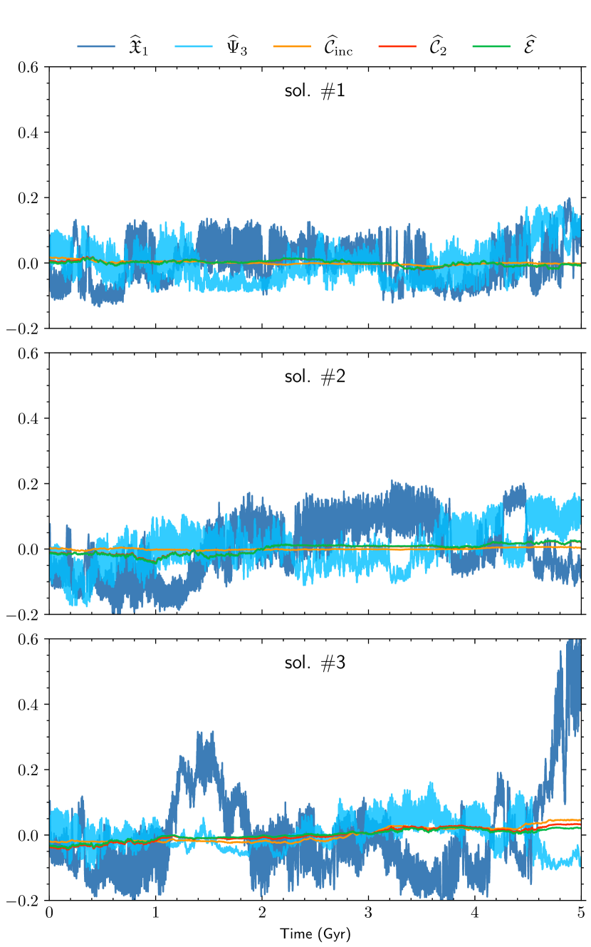
Figure 5: Time evolution over 5 Gyr of the dimensionless QIs of motions ($\widehat{\mathcal{C}}_{\mathrm{inc}},\widehat{\mathcal{C}}_{2},\widehat{\mathcal{E}}$) and of two representatives of the dimensionless action variables ($\widehat{\mathfrak{X}}_{1},\widehat{\Psi}_{3}$) for three solutions of $\mathcal{H}_{4}$, that is, sol. #1 (top), sol. #2 (middle), and sol. #3 (bottom). $\widehat{\mathcal{E}}$ stands for $\widehat{\mathcal{E}}_{4}$. The time series are low-pass filtered with a cutoff frequency of 1 Myr^-1 and the mean over 5 Gyr is subtracted.

Solution #3 in Fig. 4 represents an edge case (see Fig. 5 for its time evolution). Typically, the variances of the QIs are at least one order of magnitude smaller than those of the action variables, which allows a clear separation. Nevertheless, the distinction between the QIs and faster d.o.f. can be more difficult in two rare possibilities. Firstly, if the change in a QI accumulates continually in one direction, its variance can inflate over a long time interval. This is the case for the interval [0, 5] Gyr of sol. #3. Secondly, the variance of a variable that is typically fast can suddenly dwindle during a certain period of time, for example, $\Psi_{3}$ over the interval [1, 2] Gyr of sol. #3. In both cases, the slow subspace defined by the three last PCs can move away from the QI subspace due to the contamination by d.o.f. that are typically faster. This is reflected in the mismatch of QI₃ and PC₆ on the last two time intervals of sol. #3 in Fig. 4. We remark that PC_8,7 are still relatively close to QI_1,2, which indicates that the slowest 2-dimensional subspace spanned by PC_8,7 still resides inside the QI subspace. It should be stressed that this disagreement between QIs and PCs does not mean that the QIs are not slow variables in this case. The mismatch has a clear dynamical origin instead. The resonance tables of this work have been retrieved from a single, very long orbital solution, with the idea that its time statistics is representative of the ensemble statistics over a set of initially very close solutions [19]. Therefore, the QIs derived from these tables characterize the dynamics in a global sense. The network of resonances can temporarily change in an appreciable way along specific solution, or be very particular along rare orbital solutions. In these cases, a mismatch between the last PCs and the present QIs may naturally arise. Moreover, the contamination of the QIs by d.o.f. that are typically faster may also be expected from the previously mentioned lack of a strong hierarchical structure of the slow variables. The Lyapunov spectrum in Fig. 1a shows that the marginal distributions of the exponents $\lambda_{5}$ and $\lambda_{6}$, for example, are not separate but overlap each other.

V.2.3 Distance between the subspaces of PCs and QIs

The closeness of the two 3-dimensional linear subspaces $V_{\mathrm{PCs}},V_{\mathrm{QIs}}\subset\mathbb{R}^{8}$ spanned by the sets of vectors $S_{\mathrm{PCs}}$ and $S_{\mathrm{QIs}}$, respectively, can be quantitatively measured in terms of a geometric distance. This can be formulated using the principal (canonical) angles [55, 56, 57].

Let $A$ and $B$ be two sets of $m\leq n$ independent vectors in $\mathbb{R}^{n}$. The principal vectors $(\bm{p}_{k},\bm{q}_{k})_{k=1}^{m}$ are defined recursively as solutions to the optimization problem:

maximize $$\bm{p}\cdot\bm{q}$$ (29)

  $$\bm{p}\in\operatorname{span}(A),\enspace\bm{q}\in\operatorname{span}(B),$$

subject to $$\|\bm{p}\|=1,\enspace\|\bm{q}\|=1,$$

$$\bm{p}\cdot\bm{p}_{i}=0,\enspace\bm{q}\cdot\bm{q}_{i}=0,\enspace i=1,\dots,k-1,$$

for $k=1,\dots,m$. The principal angles $0\leq\theta_{1}\leq\dots\leq\theta_{m}\leq\pi/2$ between the two subspaces $\operatorname{span}(A)$ and $\operatorname{span}(B)$ are then defined by

$$\cos\theta_{k}=\bm{p}_{k}\cdot\bm{q}_{k},\quad k=1,\dots,m.$$ (30)

The principal angle $\theta_{1}$ is the smallest angle between all pairs of unit vectors in span($A$) and span($B$); the principal angle $\theta_{2}$ is the smallest angle between all pairs of unit vectors that are orthogonal to the first pair; and so on. Given the matrices defining the two subspaces, the principal angles can be computed from the singular value decomposition of their correlation matrix. The result is the canonical correlation matrix $\textrm{diag}(\cos\theta_{1},\dots,\cos\theta_{m})$. This cosine-based method is often ill-conditioned for small angles. In such case, a sine-based algorithm can be employed [58]. In this work, we use the combined technique detailed in Ref. [59].

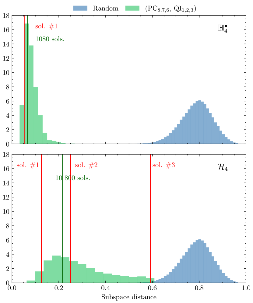
Figure 6: PDF of the distance between two random 3-dimensional linear subspaces of $\mathbb{R}^{8}$ (blue, $10^{5}$ draws) compared with the PDF of the distance between the two subspaces $V_{\mathrm{PCs}}$ (PC_8,7,6) and $V_{\mathrm{QIs}}$ (QI_1,2,3) arising from the time interval [0, 5] Gyr of 1080 solutions of $\mathbb{H}_{4}^{\bullet}$ (top) and 10 800 solutions of $\mathcal{H}_{4}$ (bottom) (green). For each model, the subspace distance from the same time interval of representative solutions (vertical red lines) and of the aggregated sample of all the solutions (vertical dark green line) are indicated. The subspace distance is given by Eq. (31).

Once the principal angles have been introduced, different metrics can be defined to measure the distance between two subspaces. In this work, we choose the normalized chordal distance [57]:

$$d(A,B)=\left(\frac{1}{m}\sum_{k=1}^{m}\sin^{2}\theta_{k}\right)^{1/2}.$$ (31)

The distance is null if $A$ and $B$ are the same subspace and equal to $1$ when they are orthogonal. We use this metric to show that the subspace closeness suggested by Figs. 3 and 4 is indeed statistically significantly. More precisely, we provide evidence against the null hypothesis that the distribution of distances between $V_{\mathrm{PCs}}$ and $V_{\mathrm{PCs}}$, arising from the $\mathbb{H}_{4}^{\bullet}$ and $\mathcal{H}_{4}$ dynamics, coincides with that of randomly drawn 3-dimensional subspaces of $\mathbb{R}^{8}$. The PDF of the distance between two random 3-dimensional subspaces of $\mathbb{R}^{8}$ is shown in Fig. 6 in blue (such random subspaces can be easily generated by sampling sets of 3 vectors uniformly on the unit $7$-sphere [60]). While the range of possible distances is [0,1], the distribution concentrates on the right-hand side of the interval, with a probability of approximately 99.3% that the distance is larger than 0.6. In this regard, we remark that the notion of distance in high-dimensional spaces is very different from our intuition in a 3-dimensional world. If we draw randomly two vectors in a very high-dimensional space, it is extremely likely that they will be close to mutual orthogonality.

The upper panel of Fig. 6 shows in green the PDF of the distance between $V_{\mathrm{PCs}}$ and $V_{\mathrm{QIs}}$ arising from the time interval [0, 5] Gyr of the 1080 orbital solutions of model $\mathbb{H}_{4}^{\bullet}$. In the lower panel, we consider a larger ensemble of 10 800 solutions of model $\mathcal{H}_{4}$ spanning the same time interval [7], and plot the corresponding PDF of the distance between $V_{\mathrm{PCs}}$ and $V_{\mathrm{QIs}}$. In both cases, the distance stemming from the aggregated sample of all the solutions is indicated by a vertical dark green line. We also report the distances from the specific solutions considered in Figs. 3 and 4 as vertical red lines. As the PDFs of both models peak at small distances, there results a strong evidence that the distribution of distances between the subspaces spanned by the PCs and the QIs is not that of random subspaces. In this sense, the closeness of the subspaces $V_{\mathrm{PCs}}$ and $V_{\mathrm{QIs}}$ is a statistically robust result. In the case of the simplified dynamics $\mathbb{H}_{4}^{\bullet}$, the PDF peaks around a median of roughly 0.08 and has small variance. Switching to model $\mathcal{H}_{4}$, the median increases to about 0.26 and the PDF is more spread out, with a long tail toward larger distances. The differences between the PDFs of the two models follow quite naturally the discussion in Sect. V.2.2: a quasi frozen hierarchy of the slowest variables for $\mathbb{H}_{4}^{\bullet}$; a larger variance for $\mathcal{H}_{4}$ related to contamination by d.o.f. that are typically faster and to variations of the resonant network with respect to the nominal solution of Gauss’s dynamics which is used to infer the QIs. Solution #3 in Fig. 4 represents in this sense an edge case of the distance distribution, while sol. #2 is a typical solution close to the PDF median.

VI Implications on long-term stability

The existence of slow variables can have crucial implications on the stability of the ISS. The QIs of motion can effectively constraint in an adiabatic way the chaotic diffusion of the planet orbits over long timescales, forbidding in general a dynamical instability over a limited time span, e.g., several billions of years. Here we give compelling arguments for such a mechanism.

Figure 7 shows the cumulative distribution function (CDF) of the first time that Mercury eccentricity reaches a value of 0.7, from the ensembles of 1080 orbital solutions of $\mathbb{H}_{4}^{\bullet}$ and $\mathbb{H}_{6}^{\bullet}$ introduced in Sect. IV.4. We recall that such a high eccentricity is a precursor of the dynamical instability (i.e., close encounters, collisions, or ejections of planets) of the ISS [6]. We also report the same CDF for the models $\mathcal{H}_{4}$ and $\mathcal{H}_{6}$, which we recently computed in Ref. [7]. One can appreciate that the time corresponding to a probability of instability of 1% is greater than 100 Gyr for the $\mathbb{H}_{4}^{\bullet}$ model, while it is about 15 Gyr for $\mathcal{H}_{4}$. At degree 6, this time still increases from 5 Gyr for $\mathcal{H}_{6}$ to about 20 Gyr in $\mathbb{H}_{6}^{\bullet}$. The dynamics arising from $\mathbb{H}_{4}^{\bullet}$ and $\mathbb{H}_{6}^{\bullet}$ can be considered as stable in an astronomical sense. Recalling that the main difference between $\mathbb{H}_{2n}^{\bullet}$ and $\mathbb{H}_{2n}$ relates to the smallest Lyapunov exponents (Fig. 1), and this is accompanied by a much slower diffusion of the QIs for $\mathbb{H}_{2n}^{\bullet}$ (Figs. 2, 10, and 11), Fig. 7 indicates that the dynamical half-life of the ISS is linked to the speed of diffusion of these slow quantities in a critical way. We stress that the slower diffusion toward the dynamical instability in the $\mathbb{H}_{2n}^{\bullet}$ model derives from neglecting the external forcing mainly exerted by Saturn, Uranus, and Neptune.

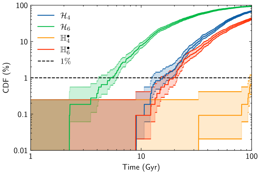
Figure 7: Cumulative distribution function of the first time that Mercury eccentricity reaches a value of 0.7, from 1080 orbital solutions of different models over 100 Gyr. The shaded regions represent the 90% piecewise confidence intervals from bootstrap.

We also observe that, to a linear approximation, the knowledge of $\mathcal{C}_{\textnormal{\scriptsize inc}}$ and $\mathcal{E}_{2}$ allows us to bound the variations of the action variables $\bm{\mathfrak{X}},\bm{\Psi}$. Recalling that the actions are positive quantities, from Eq. (19) one sees that fixing a value of $\mathcal{C}_{\textnormal{\scriptsize inc}}$ puts an upper bound to the variations of the inclination actions $\bm{\Psi}$. As a consequence, at degree 2 in eccentricities and inclinations, fixing a value of the QI

$$\mathcal{E}_{2}=\bm{\gamma}_{3}\cdot\bm{I}=\bm{\gamma}^{\textnormal{\scriptsize ecc}}_{3}\cdot\bm{\mathfrak{X}}+\bm{\gamma}^{\textnormal{\scriptsize inc}}_{3}\cdot\bm{\Psi},$$ (32)

with $\bm{\gamma}_{3}=(\bm{\gamma}^{\textnormal{\scriptsize ecc}}_{3},\bm{\gamma}^{\textnormal{\scriptsize inc}}_{3})$, also bounds the upper variations of the eccentricity actions $\bm{\mathfrak{X}}$, since the components of $\bm{\gamma}^{\textnormal{\scriptsize ecc}}_{3}$ have all the same sign, as those of $\bm{\gamma}^{\textnormal{\scriptsize inc}}_{3}$ (see Appendix B). This is an important point, as we state in Sect. I that the lack of any bound on the chaotic variations of the planet orbits is one of the reasons that complicate the understanding of their long-term stability. We remark that the secular planetary phase space can be bound by fixing the value of the total AMD, that is, $\mathcal{C}_{\textnormal{\scriptsize ecc}}+\mathcal{C}_{\textnormal{\scriptsize inc}}$ [47]. A statistical study of the density of states that are a priori accessible can then be realized [61]. It is not, however, fully satisfying to consider a fixed value of total AMD of the ISS, as we show that $\mathcal{C}_{\textnormal{\scriptsize ecc}}$ is changed by some of the leading resonances of the Hamiltonian, as a result of the eccentricity forcing mainly exerted by Jupiter through the mode $g_{5}$. Moreover, the destabilization of the ISS consists indeed in a large transfer of eccentricity AMD, $\mathcal{C}_{\textnormal{\scriptsize ecc}}$, from the outer system to the inner planets through the resonance $g_{1}-g_{5}$ [5, 36, 6, 62]. It should be noted that $\mathcal{C}_{\textnormal{\scriptsize ecc}}$ can still be consider as a slow quantity with respect to an arbitrary function of the action variables, as it is only changed by the subset of the leading resonances involving the external mode $g_{5}$. This slowness has indeed been observed on stable orbital solutions of the Solar System [47] and supports the statistical hypothesis in Ref. [61] that allows one to obtain a very reasonable first guess of the long-term PDFs of the eccentricities and inclinations of the inner planets.

The emerging picture explains the statistical stability of the ISS over billions of years in a physically intuitive way. The chaotic behavior of the planet orbits arises from the interaction of a number of leading resonant harmonics of the Hamiltonian, which determine the Lyapunov time. The strongest resonances are characterized by some exact symmetries, which are only broken by weak resonant interactions. These quasi-symmetries naturally give birth to QIs of motion, quantities that diffuse much more slowly than the LL action variables, constraining the variations of the orbits. The long dynamical half-life of the ISS is connected to the speed of this diffusion, which eventually drives the system to the instability. It should be stressed that, besides the speed of diffusion, the lifetime of the inner orbits also depends on the initial distance of the system from the instability boundary defined by the resonance $g_{1}-g_{5}$. This geometric aspect includes the stabilizing role of general relativity [5, 6], which moves the system away from the instability boundary by 0.43${}^{\prime\prime}\,{\textrm{yr}}^{-1}$, and the destabilizing effect of terms of degree 6 in eccentricities and inclinations of the planets [7].

VII Discussion

This work introduces a framework that naturally justifies the statistical stability shown by the ISS over a timescale comparable to its age. Considering a forced secular model of the inner planet orbits, the computation of the Lyapunov spectrum indicates the existence of very different dynamical timescales. Using the computer algebra system TRIP, we systematically analyze the Fourier harmonics of the Hamiltonian that become resonant along a numerically integrated orbital solution spanning 5 Gyr. We uncover three symmetries that characterize the strongest resonances and that are broken by weak resonant interactions. These quasi-symmetries generate three QIs of motion that represent slow variables of the secular dynamics. The size of the leading symmetry-breaking resonances suggests that the QIs are related to the smallest Lyapunov exponents. The claim that the QIs are among the slowest d.o.f. of the dynamics constitutes the central point of this work. On the one hand, it is supported by the analysis of the underlying Hamiltonian $\mathbb{H}_{2n}^{\bullet}$, in which one neglects the forcing mainly exerted by Saturn, Uranus, and Neptune and, as a consequence, the diffusion of the QIs is greatly reduced. On the other hand, the geometric framework established by the PCA of the orbital solutions independently confirms that the QIs are statistically the slowest linear variables of the dynamics. We give strong evidence that the QIs of motion play a critical role in the statistical stability of the ISS over the Solar System lifetime, by adiabatically constraining the long-term chaotic diffusion of the orbits.

VII.1 Inner Solar System among classical quasi-integrable systems

It is valuable to contextualize the dynamics of the ISS in the class of classical quasi-integrable systems. A comparison with the Fermi-Pasta-Ulam-Tsingou problem, in particular, deserves to be made. This concerns the dynamics of a one-dimensional chain of identical masses coupled by nonlinear springs. For weak nonlinearity, the normal modes of oscillation remain far from the energy equipartition expected from statistical mechanics for a very long time [13]. One way to explain the lack of energy equipartition reported by Fermi and collaborators is through the closeness of the FPUT problem to the integrable Toda dynamics [63, 64, 65]. This translates in a very slow thermalization of the action variables of the Toda problem and of the corresponding integrals of motion along the FPUT flow [65, 66, 67, 15, 68, 69]. In the framework of the present study, the very long dynamical half-life of the ISS is also likely to be the result of the slow diffusion of some dynamical quantities, the QIs of motion. We find, in particular, an underlying Hamiltonian $\mathbb{H}_{2n}^{\bullet}$ for which this diffusion is greatly reduced, as a consequence of neglecting the forcing mainly exerted by Saturn, Uranus, and Neptune. This results in a dynamics that can be considered as stable in an astronomical sense. We stress that, differently from the FPUT problem, $\mathbb{H}_{2n}^{\bullet}$ is not integrable as the Toda Hamiltonian. It is indeed chaotic and shares with the original Hamiltonian $\mathbb{H}_{2n}$ the leading Lyapunov exponents. The QIs that we find in this work are only a small number of functions of the action-angle variables of the integrable LL dynamics, and are related to the smallest Lyapunov exponents of the dynamics. Our study suggests that in the FPUT problem the very slow thermalization occurring beyond the Lyapunov time might be understood in terms of combinations of the Toda integrals of motion diffusing over very different timescales.

The long-term diffusion in chaotic quasi-integrable systems should be generally characterized by a broad range of timescales that results from the progressive, hierarchical breaking of the symmetries of the underlying integrable problem by resonant interactions [70, 71, 72]. A hierarchy of Lyapunov exponents spanning several orders of magnitude, in particular, should be common among this class of systems [e.g., 73].

VII.2 Methods

The long-term dynamics of the ISS is described by a moderate but not small number of d.o.f., which places it far from the typical application fields of celestial mechanics and statistical physics. The first discipline often studies dynamical models with very few degrees of freedom, while the second one deals with the limit of a very large number of bodies. Chaos also requires a statistical description of the inner planet orbits. But the lack of a statistical equilibrium, resulting from a slow but ceaseless diffusion of the system, places the ISS outside the standard framework of ergodic theory. The kind of approach we develop in this work is heavily based on computer algebra, in terms of systematic series expansion of the Hamiltonian, manipulation of the truncated equations of motion, extraction of given Fourier harmonics, retrieval of polynomial roots, etc. [4, 19]. This allows us to introduce QIs of motion in a 16-dimensional dynamics by analyzing how action-space symmetries are progressively broken by resonant interactions. Our effective method based on the time statistics of resonances arising along a single, very long numerical integration is alternative to formal approaches that define QIs via series expansions [e.g. 74, 75]. The practical usefulness of these formal expansions for a dynamics that covers an intricate, high-dimensional network of resonances seems indeed doubtful. Through the retrieval of the half-widths of the symmetry-breaking resonances, computer algebra also permits us to extend the correspondence between the Lyapunov spectrum and the spectrum of resonances well beyond the standard relation linking the Lyapunov time to the strongest resonances.

In the context of dynamical systems with a number of d.o.f. that is not small, this work also considers an approach based on PCA. The role of this statistical technique can be twofold. We use PCA as an independent test to systematically validate the slowness of the QIs. While being introduced semi-analytically as dynamical quantities that are not affected by the leading resonances, they can indeed be related to the last PCs. By extension, the first PCs should probe the directions of the main resonances. This leads to a second potential application of the PCA, which should offer a way to retrieve the principal resonant structure of a dynamical system. In this sense, PCA represents a tool to systematically probe numerical integrations of a complex dynamics and distill important hidden insights. We emphasize that PCA is the most basic linear technique of dimensionality reduction and belongs to the more general class of the unsupervised learning algorithms. There are more sophisticated methods of feature extraction that can be more robust [e.g. 77, 78] and can incorporate nonlinearity [79]. These methods are often less intuitive to understand, less straightforward to apply, and harder to interpret than PCA. Yet, they might be more effective and worth pursuing for future works.

With long-term numerical integration and a computer algebra system at one’s disposal, the entire strategy we develop in this work can in principle be applied to other planetary systems and quasi-integrable Hamiltonian dynamics with a moderate number of d.o.f.

Appendix A Lyapunov spectrum

(a) $\mathcal{H}_{4}$: Single orbital solution

(b) $\mathcal{H}_{4}$: Relative numerical errors

ciao

Figure 8: (a) Positive FT-LCEs of Hamiltonian $\mathcal{H}_{4}$ and corresponding characteristic timescales for a single initial condition and an ensemble of 150 random sets of initial tangent vectors. The bands represent the [5th, 95th] percentile range of the marginal PDFs. The lines denote the distribution medians. (b) Medians of the relative numerical errors $\epsilon_{i}$ on the FT-LCEs $\lambda_{i}$, as defined in Eq. (33), for the ensemble of 150 orbital solution of Fig. 1a.

Convergence.

We perform two tests to address the convergence of our implementation of the Benettin et al. [43] method. We first compute the FT-LCEs for a single initial condition of $\mathcal{H}_{4}$ and an ensemble of 150 different random sets of initial tangent vectors. Figure 7a shows the [5th, 95th] percentile range of the resulting marginal distributions of the positive FT-LCEs over a time span of 10 Gyr. The distributions shrink with increasing time, eventually collapsing on single time-dependent values. In this asymptotic regime, the Benettin et al. [43] algorithm loses memory of the initial tangent vectors and purely retrieves the FT-LCEs as defined in Eq. (10). Therefore, Fig. 1a shows asymptotically the dependence of the FT-LCEs on the initial condition $\bm{z}_{0}$ and represents their statistical distribution over the phase-space domain explored by the dynamics in a non-ergodic way. The convergence of the computation is clearly slower for smaller exponents, but a comparison with Fig. 1a indicates that, even in the case of $\lambda_{8}$, the numerical uncertainty on the FT-LCEs of each orbital solution at 10 Gyr is negligible with respect to the width of their ensemble distributions.

To quantitatively estimate the numerical precision on the computed FT-LCEs, we exploit the symmetry of the spectrum stated in Eq. (9). For a single orbital solution, the relative numerical error on each exponent $\lambda_{i}$ can be estimated as

$$\epsilon_{i}=\left|\frac{\Delta\lambda_{i}}{\lambda_{i}}\right|.$$ (33)

We plot in Fig. 7b the medians of $\epsilon_{i}$ for the ensemble of 150 orbital solutions of Fig. 1a. The relative errors decrease asymptotically with time, as expected. Even in the case of the smallest exponent, $\lambda_{8}$, the median error is less than 10% at 10 Gyr.

Hamiltonian $\mathcal{H}_{6}$.

We compute for comparison the FT-LCEs of the forced ISS truncated at degree 6 in eccentricities and inclinations, that is, $\mathcal{H}_{6}$. We consider 150 stable orbital solutions with initial conditions very close to the nominal values of Gauss’s dynamics and random sets of initial tangent vectors, as we do for the truncation at degree 4. Figure 9 shows the [5th, 95th] percentile range of the marginal PDF of each FT-LCE estimated from the ensemble of solutions. Apart from being somewhat larger, the asymptotic distributions of the exponents are very similar to those of $\mathcal{H}_{4}$ shown in Fig. 1a.

Appendix B Vectors $\bgamma_{1}$, $\bgamma_{2}$, $\bgamma_{3}$

We report here the explicit expressions of the vectors $(\bm{\gamma}_{i})_{i=1}^{3}$. We first give the components of the vector $\bm{\omega}_{\scaleto{\textsc{LL}}{4pt}}$ of the fundamental precession frequencies of the inner orbits in the forced Laplace-Lagrange dynamics (including the leading correction of general relativity) [4]:

$$\bm{\omega}_{\scaleto{\textsc{LL}}{4pt}} =(\bm{g}_{\scaleto{\textsc{LL}}{4pt}},\bm{s}_{\scaleto{\textsc{LL}}{4pt}})\approx$$ (34)

$$(5.87,7.46,17.4,18.1,-5.21,-6.59,-18.8,-17.7),$$

in units of ${\textrm{arcsec yr}}^{-1}$ (see [80, 81, 82] for comparison with the frequencies of the Laplace-Lagrange dynamics of the entire Solar System). One then has

$$\bm{\gamma}_{1} =(\bm{0}_{4},\bm{1}_{4})=(0,0,0,0,1,1,1,1),$$ (35)

$$\bm{\gamma}_{2} =(0,0,-1,-1,1,1,2,2),$$

$$\bm{\gamma}_{3} =-\bm{\omega}_{\scaleto{\textsc{LL}}{4pt}}+g_{5}\bm{1}_{8}\approx$$

$$(-1.61,-3.20,-13.2,-13.9,9.47,10.8,23.0,22.0),$$

with the components of $\bm{\gamma}_{3}$ in units of ${\textrm{arcsec yr}}^{-1}$. We recall that $g_{5}\approx 4.257$${}^{\prime\prime}\,{\textrm{yr}}^{-1}$ is a constant in the forced model of the ISS. The corresponding unit vectors $(\widehat{\bm{\gamma}}_{i})_{i=1}^{3}$ are given by

$$\widehat{\bm{\gamma}}_{1} =(0,0,0,0,1,1,1,1)/2,$$ (36)

$$\widehat{\bm{\gamma}}_{2} =(0,0,-1,-1,1,1,2,2)/2\sqrt{3},$$

$$\widehat{\bm{\gamma}}_{3} \approx(-0.04,-0.08,-0.33,-0.35,0.24,0.27,0.58,0.55).$$

Since $1/2\sqrt{3}\approx 0.289$, the components of $\widehat{\bm{\gamma}}_{3}$ are only a few percent away from those of $\widehat{\bm{\gamma}}_{2}$. Therefore, along stable orbital solutions with typical bounded variations of the Mercury-dominated action variable $\mathfrak{X}_{1}$, the two quantities $\mathcal{C}_{2}$ and $\mathcal{E}_{2n}$ exhibit very similar time evolutions. This is not the case anymore when Mercury orbit reaches high eccentricities.

Figure 9: Positive FT-LCEs $\lambda_{i}$ of Hamiltonian $\mathcal{H}_{6}$ and corresponding characteristic timescales $\lambda_{i}^{-1}$. The bands represent the [5th, 95th] percentile range of the marginal PDFs estimated from an ensemble of 150 stable orbital solutions with very close initial conditions. The lines denote the distribution medians.

Appendix C Ensemble distributions of the quasi-integrals over time

To retrieve the long-term statistical behavior of the QIs, we consider the ensembles of 1080 numerical integrations of the dynamical models $\mathcal{H}_{4}$ and $\mathcal{H}_{6}$, with very close initial conditions and spanning 100 Gyr in the future, that have been presented in Ref. [7]. We also consider the similar ensembles of solutions for the simplified Hamiltonians $\mathbb{H}_{4}^{\bullet}$ and $\mathbb{H}_{6}^{\bullet}$ that we introduce in Sect. IV.4. We report in Fig. 10 the time evolution of the ensemble PDFs of the low-pass filtered dimensionless QIs and dimensionless actions $\mathfrak{X}_{1},\Psi_{3}$ for the different models (the cutoff frequency of the time filter is set to 1 Myr^-1, as in Sec. IV.2). More precisely, to highlight the growth of the statistical dispersion, we consider at each time the PDF of the signed deviation from the ensemble mean, so that all the plotted distributions have a null mean. At each time, the PDF estimation takes into account only the stable orbital solutions, that is, those solutions whose running maximum of Mercury eccentricity is smaller than 0.7 [7]. Figure 10 shows that the QIs are indeed slow quantities when compared to the LL action variables. The growth of the QI dispersion is detailed in Fig. 11, where we report the time evolution of the interquartile range (IQR) of their distributions. After a transient phase lasting about 100 Myr and characterized by the exponential separation of close trajectories, the time growth of the IQR follows a power law typical of diffusion processes. Figures 10 and 11 clearly show the slower diffusion of $\mathcal{C}_{\textnormal{\scriptsize inc}}$ and $\mathcal{C}_{2}$ in the model $\mathbb{H}_{2n}^{\bullet}$ when compared to $\mathcal{H}_{2n}$. We recall that $\mathcal{E}_{2n}^{\bullet}$ is an exact integral of motion for the model $\mathbb{H}_{2n}^{\bullet}$ (see Sect. IV.4) and its PDF has null dispersion.

Figure 10: Time evolution over 100 Gyr of the PDF of the signed deviation from the mean of the low-pass filtered dimensionless QIs and dimensionless actions $\mathfrak{X}_{1},\Psi_{3}$. Estimation from an ensemble of 1080 numerical orbital solutions for different models ($\mathcal{H}_{4}$, $\mathcal{H}_{6}$, $\mathbb{H}_{4}^{\bullet}$, and $\mathbb{H}_{6}^{\bullet}$). First row: $\widehat{\mathcal{C}}_{\textnormal{\scriptsize inc}}$. Second row: $\widehat{\mathcal{C}}_{2}$. Third row: $\widehat{\mathcal{E}}_{4}$ ($\mathcal{H}_{4}$) and $\widehat{\mathcal{E}}_{6}$ ($\mathcal{H}_{6}$). Fourth row: $\widehat{\mathfrak{X}}_{1}$. Fifth row: $\widehat{\Psi}_{3}$. The time of each curve is color coded. At each time, the estimation only takes into account stable solutions, that are those with a running maximum of Mercury eccentricity smaller than 0.7. The quantity $\widehat{\mathcal{E}}_{2n}^{\bullet}$ is an exact integral of motion for the model $\mathbb{H}_{2n}^{\bullet}$ and its PDF has null dispersion.

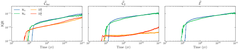
Figure 11: Time evolution of the interquartile range (IQR) of the ensemble PDFs of the QIs shown in Fig. 10. Left: $\widehat{\mathcal{C}}_{\textnormal{\scriptsize inc}}$. Middle: $\widehat{\mathcal{C}}_{2}$. Right: $\widehat{\mathcal{E}}_{4}$ ($\mathcal{H}_{4}$) and $\widehat{\mathcal{E}}_{6}$ ($\mathcal{H}_{6}$). The quantity $\widehat{\mathcal{E}}_{2n}^{\bullet}$ is an exact integral of motion for the model $\mathbb{H}_{2n}^{\bullet}$ and its PDF has a null IQR.

References

- Laskar [1989] J. Laskar, A numerical experiment on the chaotic behaviour of the solar system, Nature (London) 338, 237 (1989).
- Laskar [1990a] J. Laskar, The chaotic motion of the solar system - A numerical estimate of the size of the chaotic zones, Icarus 88, 266 (1990a).
- Sussman and Wisdom [1992] G. J. Sussman and J. Wisdom, Chaotic evolution of the solar system, Science 257, 56 (1992).
- Mogavero and Laskar [2021] F. Mogavero and J. Laskar, Long-term dynamics of the inner planets in the Solar System, Astronomy and Astrophysics 655, A1 (2021), arXiv:2105.14976 [astro-ph.EP] .
- Laskar [2008] J. Laskar, Chaotic diffusion in the Solar System, Icarus 196, 1 (2008), arXiv:0802.3371 .
- Laskar and Gastineau [2009] J. Laskar and M. Gastineau, Existence of collisional trajectories of Mercury, Mars and Venus with the Earth, Nature (London) 459, 817 (2009).
- Hoang et al. [2022] N. H. Hoang, F. Mogavero, and J. Laskar, Long-term instability of the inner Solar system: numerical experiments, Monthly Notices of the RAS 514, 1342 (2022), arXiv:2205.04170 [astro-ph.EP] .
- Batygin et al. [2015] K. Batygin, A. Morbidelli, and M. J. Holman, Chaotic Disintegration of the Inner Solar System, Astrophys. J. 799, 120 (2015), arXiv:1411.5066 [astro-ph.EP] .
- Woillez and Bouchet [2020] E. Woillez and F. Bouchet, Instantons for the Destabilization of the Inner Solar System, Phys. Rev. Lett. 125, 021101 (2020), arXiv:1910.04005 [nlin.CD] .
- Note [1] The dynamics truncated at degree 4 produces nevertheless the same chaos of the full system, as measured by the finite-time maximum Lyapunov exponent [19].
- Milani and Nobili [1992] A. Milani and A. M. Nobili, An example of stable chaos in the Solar System, Nature (London) 357, 569 (1992).
- Morbidelli and Froeschlé [1996] A. Morbidelli and C. Froeschlé, On the Relationship Between Lyapunov Times and Macroscopic Instability Times, Celestial Mechanics and Dynamical Astronomy 63, 227 (1996).
- Fermi et al. [1955] E. Fermi, P. Pasta, S. Ulam, and M. Tsingou, Studies of Nonlinear Problems, Tech. Rep. (Los Alamos National Laboratory, 1955).
- Lam and Kurchan [2014] K.-D. N. T. Lam and J. Kurchan, Stochastic Perturbation of Integrable Systems: A Window to Weakly Chaotic Systems, Journal of Statistical Physics 156, 619 (2014).
- Goldfriend and Kurchan [2019] T. Goldfriend and J. Kurchan, Equilibration of quasi-integrable systems, Phys. Rev. E 99, 022146 (2019), arXiv:1810.06121 [cond-mat.stat-mech] .
- Note [2] This resonance involves the fundamental precession frequencies of Mercury and Jupiter perihelia [5, 36, 62].
- Laskar [1996] J. Laskar, Large Scale Chaos and Marginal Stability in the Solar System, Celestial Mechanics and Dynamical Astronomy 64, 115 (1996).
- Note [3] “At each stage of its evolution, the system should have a time of stability comparable with its age” [17].
- Mogavero and Laskar [2022] F. Mogavero and J. Laskar, The origin of chaos in the Solar System through computer algebra, Astronomy and Astrophysics 662, L3 (2022), arXiv:2205.03298 [astro-ph.EP] .
- Laskar et al. [2004] J. Laskar, P. Robutel, F. Joutel, M. Gastineau, A. C. M. Correia, and B. Levrard, A long-term numerical solution for the insolation quantities of the Earth, Astronomy and Astrophysics 428, 261 (2004).
- Morbidelli [2002] A. Morbidelli, Modern celestial mechanics: aspects of solar system dynamics (Taylor & Francis, 2002).
- Gauss [1818] C. F. Gauss, Determinatio attrationis, quam in punctum quodvis positionis datae exerceret planeta, SI eius massa per tota orbitam, ratione temporis, quo singulae partes describuntur, uniformiter errat dispertita (Heinrich Dieterich, Göttingen, 1818).
- Laskar [1991] J. Laskar, Analytical framework in Poincaré variables for the motion of the solar system, in Predictability, Stability, and Chaos in N-Body Dynamical Systems, NATO Advanced Study Institute (ASI) Series B, Vol. 272, edited by A. Roy (Plenum Press, New York, 1991) pp. 93–114.
- Laskar and Robutel [1995] J. Laskar and P. Robutel, Stability of the Planetary Three-Body Problem. I. Expansion of the Planetary Hamiltonian, Celestial Mechanics and Dynamical Astronomy 62, 193 (1995).
- Gastineau and Laskar [2011] M. Gastineau and J. Laskar, Trip: A computer algebra system dedicated to celestial mechanics and perturbation series, ACM Commun. Comput. Algebra 44, 194 (2011).
- Gastineau and Laskar [2021] M. Gastineau and J. Laskar, TRIP 1.4.120, TRIP Reference manual (IMCCE, Paris Observatory, 2021).
- Note [4] represents the exponential operator and stands for the imaginary unit. The overline on variables denotes complex conjugate.
- Hoang et al. [2021] N. H. Hoang, F. Mogavero, and J. Laskar, Chaotic diffusion of the fundamental frequencies in the Solar System, Astronomy and Astrophysics 654, A156 (2021), arXiv:2106.00584 [astro-ph.EP] .
- Laskar [1988] J. Laskar, Secular evolution of the solar system over 10 million years, Astronomy and Astrophysics 198, 341 (1988).
- Laskar [2005] J. Laskar, Frequency map analysis and quasiperiodic decompositions, in Hamiltonian Systems and Fourier Analysis: New Prospects For Gravitational Dynamics, edited by D. Benest, C. Froeschlé, and E. Lega (Cambridge Scientific Publishers Ltd, Cambridge, 2005) pp. 93–114, arXiv:math/0305364 .
- Oseledec [1968] V. I. Oseledec, A multiplicative ergodic theorem. Lyapunov characteristic numbers for dynamical systems, Trans.Moscow Math.Soc. 19, 197 (1968).
- Eckmann and Ruelle [1985] J. P. Eckmann and D. Ruelle, Ergodic theory of chaos and strange attractors, Reviews of Modern Physics 57, 617 (1985).
- Gaspard [1998] P. Gaspard, Chaos, Scattering and Statistical Mechanics, Cambridge Nonlinear Science Series (Cambridge University Press, 1998).
- Skokos [2010] C. Skokos, The Lyapunov characteristic exponents and their computation, in Dynamics of Small Solar System Bodies and Exoplanets, edited by J. J. Souchay and R. Dvorak (Springer Berlin Heidelberg, Berlin, Heidelberg, 2010) p. 63–135.
- Laskar [1994] J. Laskar, Large-scale chaos in the solar system., Astronomy and Astrophysics 287, L9 (1994).
- Batygin and Laughlin [2008] K. Batygin and G. Laughlin, On the Dynamical Stability of the Solar System, Astrophys. J. 683, 1207 (2008), arXiv:0804.1946 [astro-ph] .
- Note [5] The FT-LCEs do not depend on any tangent vector .
- Note [6] All the initial conditions mentioned in this work are sampled from a multidimensional Gaussian distribution that is centered at the nominal initial conditions of Gauss’s dynamics [4, Appendix D] and has a relative width of (see [19, Appendix C] and [7, Sect. 3] for details).
- Morbidelli and Giorgilli [1995] A. Morbidelli and A. Giorgilli, On a connection between KAM and Nekhoroshev’s theorems, Physica D Nonlinear Phenomena 86, 514 (1995).
- Laskar [1992] J. Laskar, A Few Points on the Stability of the Solar System (lecture), in Chaos, Resonance, and Collective Dynamical Phenomena in the Solar System, IAU Symposium, Vol. 152, edited by S. Ferraz-Mello (Kluwer Academic Publishers, Dordrecht, 1992) p. 1.
- Brown and Rein [2020] G. Brown and H. Rein, A Repository of Vanilla Long-term Integrations of the Solar System, Research Notes of the American Astronomical Society 4, 221 (2020), arXiv:2012.05177 [astro-ph.EP] .
- Benettin et al. [1978] G. Benettin, L. Galgani, A. Giorgilli, and J. M. Strelcyn, All Lyapunov characteristic numbers are effectively computable., Academie des Sciences Paris Comptes Rendus Serie B Sciences Physiques 286, 431 (1978).
- Benettin et al. [1980] G. Benettin, L. Galgani, A. Giorgilli, and J. M. Strelcyn, Lyapunov characteristic exponents for smooth dynamical systems and for Hamiltonian systems - A method for computing all of them. I - Theory. II - Numerical application, Meccanica 15, 9 (1980).
- Chirikov [1979] B. V. Chirikov, A universal instability of many-dimensional oscillator systems, Physics Reports 52, 263 (1979).
- Laskar [1990b] J. Laskar, Systèmes de Variables et Eléments, in Modern Methods in Celestial Mechanics, edited by D. Benest and C. Froeschle (Editions Frontières, Gif -Sur-Yvette, 1990) pp. 63–87.
- Boué and Laskar [2009] G. Boué and J. Laskar, Spin axis evolution of two interacting bodies, Icarus 201, 750 (2009).
- Laskar [1997] J. Laskar, Large scale chaos and the spacing of the inner planets., Astronomy and Astrophysics 317, L75 (1997).
- Zurbenko and Smith [2018] I. G. Zurbenko and D. Smith, Kolmogorov–Zurbenko filters in spatiotemporal analysis, WIREs Computational Statistics 10, e1419 (2018).
- Correia and Laskar [2003] A. C. M. Correia and J. Laskar, Long-term evolution of the spin of Venus. II. numerical simulations, Icarus 163, 24 (2003).
- Pearson [1901] K. Pearson, LIII. On lines and planes of closest fit to systems of points in space, The London, Edinburgh, and Dublin philosophical magazine and journal of science 2, 559 (1901).
- Hotelling [1933] H. Hotelling, Analysis of a complex of statistical variables into principal components., Journal of educational psychology 24, 417 (1933).
- Jolliffe [2002] I. T. Jolliffe, Principal component analysis (Springer, 2002).
- Jolliffe and Cadima [2016] I. T. Jolliffe and J. Cadima, Principal component analysis: a review and recent developments, Philosophical Transactions of the Royal Society A: Mathematical, Physical and Engineering Sciences 374, 20150202 (2016).
- Note [7] The projection of a vector onto the subspace spanned by a set of vectors can be written in a vectorial form as , where the column space of the matrix is the subspace spanned by the set .
- Jordan [1875] C. Jordan, Essai sur la géométrie à dimensions, Bulletin de la Société mathématique de France 3, 103 (1875).
- Van Loan and Golub [1996] C. F. Van Loan and G. Golub, Matrix computations (The Johns Hopkins University Press, London, 1996).
- Ye and Lim [2016] K. Ye and L.-H. Lim, Schubert varieties and distances between subspaces of different dimensions, SIAM Journal on Matrix Analysis and Applications 37, 1176 (2016).
- Björck and Golub [1973] A. Björck and G. H. Golub, Numerical methods for computing angles between linear subspaces, Mathematics of computation 27, 579 (1973).
- Knyazev and Argentati [2002] A. V. Knyazev and M. E. Argentati, Principal angles between subspaces in an a-based scalar product: algorithms and perturbation estimates, SIAM Journal on Scientific Computing 23, 2008 (2002).
- Muller [1959] M. E. Muller, A note on a method for generating points uniformly on n-dimensional spheres, Commun. ACM 2, 19–20 (1959).
- Mogavero [2017] F. Mogavero, Addressing the statistical mechanics of planet orbits in the solar system, Astronomy and Astrophysics 606, A79 (2017), arXiv:1703.09225 [astro-ph.EP] .
- Boué et al. [2012] G. Boué, J. Laskar, and F. Farago, A simple model of the chaotic eccentricity of Mercury, Astronomy and Astrophysics 548, A43 (2012), arXiv:1210.5221 [astro-ph.EP] .
- Hénon [1974] M. Hénon, Integrals of the Toda lattice, Phys. Rev. B 9, 1921 (1974).
- Flaschka [1974] H. Flaschka, The Toda lattice. II. Existence of integrals, Phys. Rev. B 9, 1924 (1974).
- Manakov [1974] S. V. Manakov, Complete integrability and stochastization of discrete dynamical systems, Zhurnal Eksperimentalnoi i Teoreticheskoi Fiziki 67, 543 (1974).
- Ferguson et al. [1982] J. Ferguson, W. E., H. Flaschka, and D. W. McLaughlin, Nonlinear Normal Modes for the Toda Chain, Journal of Computational Physics 45, 157 (1982).
- Benettin et al. [2013] G. Benettin, H. Christodoulidi, and A. Ponno, The Fermi-Pasta-Ulam Problem and Its Underlying Integrable Dynamics, Journal of Statistical Physics 152, 195 (2013).
- Christodoulidi and Efthymiopoulos [2019] H. Christodoulidi and C. Efthymiopoulos, Stages of dynamics in the Fermi-Pasta-Ulam system as probed by the first Toda integral, Mathematics in Engineering 1, 359 (2019).
- Grava et al. [2020] T. Grava, A. Maspero, G. Mazzuca, and A. Ponno, Adiabatic Invariants for the FPUT and Toda Chain in the Thermodynamic Limit, Communications in Mathematical Physics 380, 811 (2020), arXiv:2001.08070 [math-ph] .
- Ford [1961] J. Ford, Equipartition of Energy for Nonlinear Systems, Journal of Mathematical Physics 2, 387 (1961).
- Onorato et al. [2015] M. Onorato, L. Vozella, D. Proment, and Y. V. Lvov, Route to thermalization in the -Fermi-Pasta-Ulam system, Proceedings of the National Academy of Science 112, 4208 (2015), arXiv:1402.1603 [nlin.CD] .
- Pistone et al. [2019] L. Pistone, S. Chibbaro, M. D. Bustamante, Y. V. Lvov, and M. Onorato, Universal route to thermalization in weakly-nonlinear one-dimensional chains, Mathematics in Engineering 1, 672–698 (2019).
- Malishava and Flach [2022] M. Malishava and S. Flach, Lyapunov Spectrum Scaling for Classical Many-Body Dynamics Close to Integrability, Phys. Rev. Lett. 128, 134102 (2022), arXiv:2109.01361 [nlin.CD] .
- Contopoulos [1960] G. Contopoulos, A third Integral of Motion in a Galaxy, Zeitschrift fuer Astrophysik 49, 273 (1960).
- Kruskal [1962] M. Kruskal, Asymptotic Theory of Hamiltonian and other Systems with all Solutions Nearly Periodic, Journal of Mathematical Physics 3, 806 (1962).
- Note [8] In this regard, it should be noted that a relation between QIs and Lyapunov exponents has already been highlighted in simple systems [83, 43].
- Candès et al. [2011] E. J. Candès, X. Li, Y. Ma, and J. Wright, Robust principal component analysis?, Journal of the ACM (JACM) 58, 1 (2011).
- Markopoulos et al. [2014] P. P. Markopoulos, G. N. Karystinos, and D. A. Pados, Optimal algorithms for {}-subspace signal processing, IEEE Transactions on Signal Processing 62, 5046 (2014).
- Lee and Verleysen [2007] J. A. Lee and M. Verleysen, Nonlinear dimensionality reduction, Vol. 1 (Springer, 2007).
- Brumberg and Chapront [1973] V. A. Brumberg and J. Chapront, Construction of a General Planetary Theory of the First Order, Celestial Mechanics 8, 335 (1973).
- Bretagnon [1974] P. Bretagnon, Long-period terms in the solar system, Astronomy and Astrophysics 30, 141 (1974).
- Laskar [1985] J. Laskar, Accurate methods in general planetary theory, Astronomy and Astrophysics 144, 133 (1985).
- Contopoulos et al. [1978] G. Contopoulos, L. Galgani, and A. Giorgilli, On the number of isolating integrals in Hamiltonian systems, Phys. Rev. A 18, 1183 (1978).