A Matrix-Free Newton Method

Abstract

A modification of Newton’s method for solving systems of $n$ nonlinear equations is presented. The new matrix-free method relies on a given decomposition of the invertible Jacobian of the residual into invertible sparse local Jacobians according to the chain rule of differentiation. It is motivated in the context of local Jacobians with bandwidth $2m+1$ for $m\ll n$. A reduction of the computational cost by $\mathcal{O}(\frac{n}{m})$ can be observed. Supporting run time measurements are presented for the tridiagonal case showing a reduction of the computational cost by $\mathcal{O}(n).$

Generalization yields the combinatorial Matrix-Free Newton Step problem. We prove NP-completeness and we present algorithmic components for building methods for the approximate solution. Inspired by adjoint Algorithmic Differentiation, the new method shares several challenges for the latter including the DAG Reversal problem. Further challenges are due to combinatorial problems in sparse linear algebra such as Bandwidth or Directed Elimination Ordering.

49M15, 47A05, 68N99

1 Introduction

We revisit Newton’s method [18, 25] for computing roots $x\in{\mathbb{R}}^{n}$ of differentiable multivariate vector functions $F:{\mathbb{R}}^{n}\rightarrow{\mathbb{R}}^{n}:y=F(x)$ with invertible dense Jacobians

$$F^{\prime}(x)\equiv\left(\frac{dy_{j}}{dx_{i}}\right)_{i,j=1,\ldots,n}\in{\mathbb{R}}^{n\times n}\;,$$

and where $x=(x_{i})$ and $y=(y_{i})$ for $i=1,\ldots,n.$ Approximate solutions for which $F(x)\approx 0$ are computed iteratively as

(1) $$\begin{split}\Delta x&\,\mbox{:=}\,-F^{\prime}(x)^{-1}\cdot F(x)\\ x&\,\mbox{:=}\,x+\Delta x\end{split}$$

for given starting points $x\in{\mathbb{R}}^{n}.$ Convergence after $p\geq 0$ iterations is typically defined as the norm of the residual $F(x)$ falling below some given threshold $0<\epsilon\ll 1.$ See, for example, [3, 13] for further information on Newton’s method.

We use $=$ to denote mathematical equality, $\equiv$ in the sense of “is defined as” and  :=  to represent assignment according to imperative programming. Approximate equality if denoted as $\approx$. We distinguish between partial ($\partial$) and total ($d$) derivatives. Multiplication is denoted by a dot. The dot may also be omitted in favor of a more compact notation.

The residual $F$ is usually given as a differentiable program written in some high-level programming language. Equation (1) implies that the two main ingredients of Newton’s method are the evaluation of the Jacobian $F^{\prime}(x)$ and the solution of the linear Newton system $F^{\prime}(x)\cdot\Delta x=-F(x).$ Algorithmic Differentiation (AD) [10] of $F$ yields $F^{\prime}(x)$ with machine accuracy at a computational cost of ${\mathcal{O}}(n)\cdot\text{Cost}(F).$ Subsequent direct solution of the linear Newton system yields the Newton steps $\Delta x\in{\mathbb{R}}^{n}$ at the computational cost of ${\mathcal{O}}(n^{3}).$ The overall computational cost can be dominated by either of the two parts depending on the ratio $\frac{\text{Cost}(F)}{{\cal O}(n^{2})}.$

Exploitation of special structure of $F$ can yield a significant reduction in computational cost. Consequently, this article proposes a matrix-free Newton method motivated by savings obtained for relevant scenarios. We present the fundamental idea behind the method and we discuss further generalization. In Section 2 we recall essential fundamentals of AD and we draw conclusions for the computation of Newton steps. The potential for reduction in computational cost is illustrated with the help of the practically relevant special case of banded local Jacobians in Section 3. Further generalization and formalization is the subject of Section 4. Conclusions are drawn in Section 5.

2 A Lesson from Adjoint AD

First-order AD comes in two fundamental flavors. Tangent AD yields

(2) $$\dot{y}=\dot{F}(x,\dot{x})\equiv F^{\prime}(x)\cdot\dot{x}$$

and, hence, the (dense) Jacobian with machine accuracy at ${\cal O}(n)\cdot\text{Cost}(\dot{F})$ by letting $\dot{x}$ range over the Cartesian basis of ${\mathbb{R}}^{n}.$ Adjoint AD computes

(3) $$\bar{x}=\bar{F}(x,\bar{y})\equiv F^{\prime}(x)^{T}\cdot\bar{y}\;,$$

yielding the same Jacobian up to machine accuracy at ${\cal O}(n)\cdot\text{Cost}(\bar{F})$ by letting $\bar{y}$ range over the Cartesian basis of ${\mathbb{R}}^{n}.$ Both tangent and adjoint AD are matrix-free methods in the sense that the Jacobian is not required explicitly in order to evaluate Equations (2) or (3). Both methods can be used to accumulate $F^{\prime}.$ Their costs differ according to the ratio

$${\cal R}\equiv\frac{\text{Cost}(\bar{F})}{\text{Cost}(\dot{F})}\;,$$

where, typically, ${\cal R}\geq 1.$ Hence, tangent AD is usually the method of choice for computing Jacobians of the residual in the context of Newton’s method. Sparsity of the Jacobian of the residual may change the picture [6].

Second-order tangent and adjoint AD follow naturally; see [10]. Hessians required by Newton’s method for convex optimization of objectives $f:{\mathbb{R}}^{n}\rightarrow{\mathbb{R}}$ can be computed at ${\cal O}(n)\cdot\text{Cost}(\dot{\bar{f}})$ using second-order adjoint versions $\dot{\bar{f}}$ of $f.$ Corresponding matrix-free Newton-Krylov methods [14] can be derived. They are based on the observation that the Hessian-vector products required by Krylov-subspace methods (e.g. Conjugate Gradients [11]) can be computed by a second-order adjoint $\dot{\bar{f}}$ without prior accumulation of the Hessian. The approach to be proposed in this article is different. It exploits special structure and local sparsity of $F$ instead of global propagation of tangents or adjoints.

2.1 Terminology

AD requires the given program $F$ to be differentiable. The notation from [10] is modified only slightly.

Definition 2.1 (Differentiable Program).

A differentiable program

$$F:{\mathbb{R}}^{n}\rightarrow{\mathbb{R}}^{m}:\;y\,\mbox{:=}\,F(x)$$

decomposes into a single assignment code

(4) $$v_{j}\,\mbox{:=}\,\varphi(v_{i})_{i\in P_{j}}\quad\text{for}~{}j=1,\ldots,p+m\;,$$

where $v_{i-n}=x_{i}$ for $i=1,\ldots,n$ and $y_{k}=v_{p+k}$ for $k=1,\ldots,m$ and with differentiable elemental functions $\varphi_{j},$ $j=1,\ldots,p+m,$ featuring elemental partial derivatives

$$\partial_{j,i}\equiv\frac{\partial\varphi_{j}}{\partial v_{i}}\quad\text{for}~{}i\in P_{j}\;.$$

The set of arguments of $\varphi_{j}$ (direct predecessors of $v_{j}$) is denoted by $P_{j}.$

Definition 2.2 (Direct Acyclic Graph).

Equation (4) induces a directed acyclic graph (DAG) $G=(V,E),$ $V=(X,Z,Y),$ $X\cap Z\cap Y=\varnothing,$ $E\subseteq V\times V$ such that $X=\{1-n,\ldots,0\},$ $Z=\{1,\ldots,p\},$ $Y=p+1,\ldots,p+m$ and $(i,j)\in E\Leftrightarrow i\in P_{j}.$ All edges $(i,j)$ are labelled with $\partial_{j,i}.$

Paths connecting vertices $i$ and $j$ are denoted as $(i,\ldots,j).$

Definition 2.3 (Layered DAG and Local Jacobians).

A DAG of a matrix chain product

$$F^{\prime}_{q}\cdot\ldots\cdot F^{\prime}_{1}=F^{\prime}\in{\mathbb{R}}^{m\times n}$$

of local Jacobians $F^{\prime}_{i},$ $i=1,\ldots,q$ is called layered DAG.

The DAG in Figure 1(a) is layered.

Definition 2.4 (Uniformly Layered DAG).

A layered DAG of a matrix chain product

$$F^{\prime}_{q}\cdot\ldots\cdot F^{\prime}_{1}=F^{\prime}\in{\mathbb{R}}^{n\times n}$$

is called uniformly layered DAG if $F^{\prime}_{i}\in{\mathbb{R}}^{n\times n}$ for $i=1,\ldots,q.$

The DAG in Figure 1(a) is uniformly layered.

Definition 2.5 (Invertible DAG).

We refer to a DAG of a differentiable program with invertible Jacobian $F^{\prime}\in{\mathbb{R}}^{n\times n}$ as an invertible DAG. The corresponding Newton step is defined as $(F^{\prime})^{-1}\cdot y$ for given $y\in{\mathbb{R}}^{n}.$

(a)	(b)	(c)

Figure 1: Sample DAGs

Adjoint AD can be implemented by using operator and function overloading in suitable programming languages such as C++ [9, 12, 21]. The given implementation of $F$ as a differentiable program is run in overloaded arithmetic to augment the computation of the function value with the recording of the corresponding DAG (also referred to as tape). For example, for q=2 the differentiable C++ program

⬇

for (int i=0;i<q;i++) {

x[i%2]*=x[(i+1)%2];

x[(i+1)%2]=sin(x[(i+1)%2]);

}

yields the DAG in Figure 1(a), where, $\partial_{1,-1}=\text{x[1]},$ $\partial_{3,1}=\cos(\text{x[0]}),$ and so forth. The Jacobian

$$F^{\prime}=\begin{pmatrix}\partial_{3,1}\partial_{1,-1}&\partial_{3,1}\partial_{1,0}\\ \partial_{4,1}\partial_{1,-1}&\partial_{4,1}\partial_{1,0}+\partial_{4,2}\partial_{2,0}\end{pmatrix}=\begin{pmatrix}\partial_{3,1}&0\\ \partial_{4,1}&\partial_{4,2}\end{pmatrix}\begin{pmatrix}\partial_{1,-1}&\partial_{1,0}\\ 0&\partial_{2,0}\end{pmatrix}$$

can be represented as the bipartite DAG in Figure 1(b). Both options for evaluating the adjoint

$$\left(\begin{pmatrix}\partial_{3,1}&0\\ \partial_{4,1}&\partial_{4,2}\end{pmatrix}\begin{pmatrix}\partial_{1,-1}&\partial_{1,0}\\ 0&\partial_{2,0}\end{pmatrix}\right)^{T}\begin{pmatrix}\bar{y}_{0}\\ \bar{y}_{1}\\ \end{pmatrix}=\begin{pmatrix}\partial_{1,-1}&0\\ \partial_{1,0}&\partial_{2,0}\end{pmatrix}\left(\begin{pmatrix}\partial_{3,1}&\partial_{4,1}\\ 0&\partial_{4,2}\end{pmatrix}\begin{pmatrix}\bar{y}_{0}\\ \bar{y}_{1}\\ \end{pmatrix}\right)$$

(with $\bar{y}=(0~{}1)^{T}$ and $\bar{y}=(1~{}0)^{T}$ giving the rows of the Jacobian) yield the same result. Note that the evaluation of the expression on the left-hand side requires 12 fma (${\cal O}(qn^{3})$; here $q=n=2$) while the right-hand-side expression take only 8 fma (${\cal O}(qn^{2})$). The same effect due to associativity of the chain rule of differentiation (equivalently, of matrix multiplication) is exploited by backpropagation in the context of training of artificial neural networks [7]. The adjoint can be visualized as the DAG in Figure 1(c).

A discussion of the numerous aspects of AD and of its implementation are beyond the scope of this article. The interested reader is referred to [10] for further information on the subject. Moreover, the AD community’s Web portal www.autodiff.org contains a comprehensive bibliography as well as links to various AD research and tool development efforts.

2.2 Lesson

Figure 2: Inverse DAG

How can Newton’s method benefit from lessons learned in adjoint AD? Working towards an answer to this question, the given implementation of $F$ as a differentiable program is assumed to be composed of elemental functions $F_{i}:{\mathbb{R}}^{n}\rightarrow{\mathbb{R}}^{n}:x^{i}=F_{i}(x^{i-1})$ for $i=1,\ldots,q$ as

(5) $$y=x^{q}=F(x^{0})=(F_{q}\circ\ldots\circ F_{1})(x^{0})$$

where $x^{0}=x.$ Application of the chain rule of differentiation to Equation (5) yields

(6) $$F^{\prime}(x^{0})=F^{\prime}_{q}(x^{q-1})\cdot\ldots\cdot F^{\prime}_{1}(x^{0})$$

implying

(7) $$\begin{split}\Delta x&=-F^{\prime}(x)^{-1}\cdot y\\ &=-(F^{\prime}_{q}(x^{q-1})\cdot\ldots\cdot F^{\prime}_{1}(x^{0}))^{-1}\cdot y\\ &=-F^{\prime}_{1}(x^{0})^{-1}\cdot\ldots\cdot F^{\prime}_{q}(x^{q-1})^{-1}\cdot y\;.\end{split}$$

$F^{\prime}(x)$ needs to be invertible. Invertibility of all $F^{\prime}_{i}$ follows immediately. Their (w.l.o.g.) $LU$ factorization [4] yields

(8) $$F_{i}\equiv F_{i}(x^{i-1})=L_{i}(x^{i-1})\cdot U_{i}(x^{i-1})\equiv L_{i}\cdot U_{i}$$

with lower triangular $L_{i}$ and upper triangular $U_{i}.$ In-place factorization yields $L_{i}-I_{n}+U_{i}$ at a computational cost of ${\mathcal{O}}(n^{3}).$ The matrix $I_{n}\in{\mathbb{R}}^{n\times n}$ denotes the identity in ${\mathbb{R}}^{n}.$ From Equation (7) it follows that

(9) $$\begin{split}\Delta x&=-U_{1}^{-1}\cdot L_{1}^{-1}\cdot\ldots\cdot U_{q}^{-1}\cdot L_{q}^{-1}\cdot y\\ &=-U_{1}^{-1}\cdot\left(L_{1}^{-1}\cdot\ldots\cdot\left(U_{q}^{-1}\cdot\left(L_{q}^{-1}\cdot y\right)\right)\ldots\right)\end{split}$$

yielding $2q$ linear systems to be solved as efficiently as possible in order to undercut the computational cost of the standard Newton method. The new method is matrix-free in the sense that $F^{\prime}$ is not accumulated explicitly. The analogy with adjoint AD is illustrated by Figure 2, where the reversed edges indicate products of vectors with inverse local Jacobians. For the example in Figure 1, the standard “accumulate first, then factorize” approach yields the Newton step

$$\underset{\Sigma=12}{\underbrace{\underset{{\cal O}(n^{3})~{}\hat{=}~{}3+3+1=7}{\underbrace{\underset{{\cal O}(qn^{3})~{}\hat{=}~{}5}{\underbrace{\left(\begin{pmatrix}\partial_{3,1}&0\\ \partial_{4,1}&\partial_{4,2}\end{pmatrix}\begin{pmatrix}\partial_{1,-1}&\partial_{1,0}\\ 0&\partial_{2,0}\end{pmatrix}\right)^{-1}}}\begin{pmatrix}y_{0}\\ y_{1}\end{pmatrix}}}}}$$

at the expense of $12{\footnotesize\,\text{fma}}.$ The alternative “factorize first, then accumulate” method

$$\underset{{O}(qn^{2})~{}\hat{=}~{}{6}}{\underbrace{\begin{pmatrix}\partial_{1,-1}&\partial_{1,0}\\ 0&\partial_{2,0}\end{pmatrix}^{-1}\underset{{O}(n^{2})~{}\hat{=}~{}3}{\underbrace{\left(\begin{pmatrix}\partial_{3,1}&0\\ \partial_{4,1}&\partial_{4,2}\end{pmatrix}^{-1}\begin{pmatrix}y_{0}\\ y_{1}\end{pmatrix}\right)}}}}$$

performs the same task using only $6{\footnotesize\,\text{fma}}.$ Admittedly, this example is extreme in the sense that all elemental Jacobians are already triangular. Products of their inverses with a vector can hence be computed very efficiently by simple forward or backward substitution. More realistically, the individual factors need to be transformed into triangular form first. Ideally, the exploitation of sparsity of the elemental Jacobians is expected to keep the corresponding additional effort low. However, the usual challenges faced in the context of direct methods for sparse linear algebra [4] need to be addressed. A representative special case is discussed in the next section. It illustrates the potential of the new method and it serves as motivation for further generalization in Section 4 with the aim to enable applicability to a wider range of practically relevant problems.

3 Banded Elemental Jacobians

Let all $F^{\prime}_{i}$ have (maximum) bandwidth $2m+1$ ($m$ off-diagonals) with $m\ll n.$ Their in-place $LU$ factorization as in Equation (8) yields $L_{i}-I_{n}+U_{i}$ with the same bandwidth at a computational cost of ${\mathcal{O}}(m^{2}n).$ The resulting $2q$ triangular linear systems can be solved efficiently with a cost of ${\mathcal{O}}(mn)$ by simple substitution, respectively. The total computational cost of the matrix-free Newton method can hence be estimated as ${\mathcal{O}}(qm^{2}n).$

For $F^{\prime}$ to become dense we require $q\geq\underline{q}\equiv(n-m-1)/m.$ For $q\gg\underline{q}$ the cost of computing $F^{\prime}$ can be estimated as ${\mathcal{O}}(qmn^{2}).$ A matrix chain product of length $q$ needs to be evaluated, where one factor has bandwidth $2m+1$ and the other factor becomes dense for $q\geq\underline{q}.$ Superiority of the matrix-free Newton method follows immediately for $m\ll n$ as ${\mathcal{O}}(qm^{2}n)<{\mathcal{O}}(qmn^{2}).$

In most real-world scenarios the accumulation of $F^{\prime}$ is likely to dominate the overall computational cost yielding a reduction of the computational cost of the matrix-free Newton method over the cost of the standard Newton method by $\mathcal{O}(\frac{n}{m}).$ Nevertheless, let the computational cost of a Newton step be dominated by the solution of the linear Newton system. Superiority of the matrix-free Newton method requires ${\cal O}(qm^{2}n)<{\cal O}(n^{3}),$ which will only be violated for $q>n$ assuming $n={\cal O}(m^{2}).$

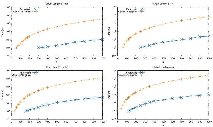
Figure 3: Tridiagonal Elemental Jacobians

Let all $F^{\prime}_{i}$ be tridiagonal. For example, this scenario occurs in the context of implicit Euler integration for one-dimensional diffusion with spacial discretization performed by central finite differences. In-place $LU$ factorization using the Thomas algorithm [23] yields the tridiagonal $L_{i}-I_{n}-U_{i}$ at a computational cost of ${\mathcal{O}}(n).$ The $2q$ linear systems in Equation (9) can be solved with a cost of the same order, respectively. The total computational cost of the matrix-free Newton method adds up to ${\mathcal{O}}(qn)<\max({\mathcal{O}}(qn^{2}),{\mathcal{O}}(n^{3})).$ The speedup of $\mathcal{O}(\frac{n}{m})=\mathcal{O}(n)$ is illustrated in Figure 3 showing the results of various experiments for a single Newton step and $q/n=0.5,1,2,4,$ $0<n\leq 10^{3}.$ The “factorize first, then accumulate” approach implements the new matrix-free Newton method. It yields the bottom line in all four sub-figures of Figure 3. The “accumulate first, then factorize” approach uses OpenBLAS’ gbmv method (www.openblas.net) for multiplying banded matrices with dense vectors. It exceeds the computational cost of the new method by roughly a factor of $n.$ Our search for a dedicated method for multiplying banded matrices turned out unsuccessful. We would expect such an algorithm to be more efficient for $q\ll n.$ Our basic reference implementation did not outperform gbmv though. Little effort went into its optimization as it would not be our method of choice for the more common scenario of $q\gg n.$

4 Towards Generalization

DAGs recorded by adjoint AD are typically neither layered nor uniform. According to Definition 2.3 the term “layered” refers to a decomposition of the DAG into a sequence of bipartite sub-DAGs representing the elemental Jacobians $F^{\prime}_{i}.$ For a DAG to be uniformly layered all layers must consist of the same number ($n$) of vertices as formally stated in Definition 2.4.

In the following we present ideas on how to make invertible DAGs uniformly layered. We formalize the corresponding methods and we prove their numerical correctness, respectively. All proofs rely on the following formulation of the chain rule of differentiation.

Lemma 4.1 (Chain Rule of Differentiation on DAG).

Let $G$ be the DAG of a differentiable program $F:{\mathbb{R}}^{n}\rightarrow{\mathbb{R}}^{m}$ as in Definition 2.2 with Jacobian

$$F^{\prime}\equiv\left(\frac{dy_{k}}{dx_{i}}\right)_{i=1,\ldots,n}^{k=1,\ldots,m}=\left(\frac{dv_{p+k}}{dv_{i-n}}\right)_{i=1,\ldots,n}^{k=1,\ldots,m}\in{\mathbb{R}}^{m}\times{\mathbb{R}}^{n}\;.$$

Then

(10) $$\frac{dv_{p+k}}{dv_{i-n}}=\sum_{(i-n,\ldots,p+k)}\prod_{(s,t)\in(i-n,\ldots,p+k)}\partial_{t,s}$$

for $i=1,\ldots,n$ and $k=1,\ldots,m.$

Proof

See [1]. $\blacksquare$

An illustrative explanation of each method is followed by its formalization and the proof of numerical correctness.

4.1 Edge Splitting

(a)	(b)

Figure 4: Edge Splitting

Consider a minor modification of the sample program from Section 2 as

⬇

for (int i=0;i<q;i++) {

x[i%2]*=x[(i+1)%2];

if (!(i%2)) x[(i+1)%2]=sin(x[(i+1)%2]);

}

For q=2, the DAG in Figure 4(a) is recorded. The edge labeled with the local partial derivative $b_{2,2}$ (=x[0] for i=1) spans two layers making the DAG not layered. We aim to transform it into a layered tripartite DAG representing the local Jacobian product $A\cdot B,$ where $A\equiv(a_{j,i})$ as well as $B\equiv(b_{j,i}).$ The $\partial_{j^{\prime},i^{\prime}}$ are replaced by $a_{j,i}$ or $b_{j,i}.$ This slight modification in the notation is expected to make he upcoming examples easier to follow.

Edge splitting makes the DAG layered by inserting $l-1=j-i-1$ dummy vertices for all edges connecting vertices in layers $i$ and $j$ (here, $l=2-0=2$ yields one additional vertex labelled $3,0$ to mark it as split vertex of edge $(0,3)$). One of the resulting new edges keeps the original label while the others are labelled with ones as in Figure 4(b) ($l-1=1$ dummy vertex). The Jacobian $F^{\prime}$ turns out to be invariant under edge splitting as an immediate consequence of the chain rule of differentiation. For example,

$$F^{\prime}=\begin{pmatrix}a_{1,1}&0\\ a_{2,1}&1\end{pmatrix}\begin{pmatrix}b_{1,1}&b_{1,2}\\ 0&b_{2,2}\end{pmatrix}=\begin{pmatrix}a_{1,1}b_{1,1}&a_{1,1}b_{1,2}\\ a_{2,1}b_{1,1}&a_{2,1}b_{1,2}+b_{2,2}\end{pmatrix}\;.$$

Invertibility of $F^{\prime}$ implies invertibility of all elemental Jacobians in the resulting uniformly layered DAG.

Definition 4.2 (Edge Splitting).

Let $G=(V,E)$ be a DAG as in Definition 2.2. An edge $(i,j)$ with label $\lambda$ is split by replacing it with two new edges $(i,k)$ and $(k,j),$ $k\not\in V,$ and labeling them with $\partial_{k,i}=\lambda$ and $\partial_{j,k}=1$ (or vice versa), respectively.

Consequences of the two choices for labelling the new edges are the subject of ongoing investigations. Both alternatives are regarded as equivalent for the purpose of the upcoming discussions.

Lemma 4.3.

Let a DAG $G$ induce an invertible Jacobian $F^{\prime}\in{\mathbb{R}}^{n\times n}$ under the chain rule of differentiation as in Lemma 4.1.

1. The Jacobian is invariant under edge splitting as in Definition 4.2.

2. If repeated edge splitting yields a uniformly layered DAG as in Definition 2.4, then the local Jacobians of each layer are invertible.

Proof

1. Equation (10) is invariant under edge splitting.

2. Let the uniformly layered DAG have depth $q.$ Equation (10) yields $F^{\prime}=F^{\prime}_{q}\cdot\ldots\cdot F^{\prime}_{1}$ and hence

   $$(F^{\prime})^{-1}=(F^{\prime}_{q}\cdot\ldots\cdot F^{\prime}_{1})^{-1}=(F^{\prime}_{1})^{-1}\cdot\ldots\cdot(F^{\prime}_{q})^{-1}$$

   implying invertibility of all $F^{\prime}_{j},$ $j=1,\ldots,q.$

$\blacksquare$

Obviously, edge splitting terminates as soon as the DAG becomes layered.

4.2 Preaccumulation

(a)	(b)

Figure 5: Preaccumulation

Making DAGs layered by edge splitting turned out to be rather straightforward. Unfortunately, the resulting layered DAGs are rarely uniform. Moreover, invertibility of the Jacobian implies that the sizes of all layers are at least equal to $n.$ We propose preaccumulation of local sub-Jacobians followed by the decomposition of the resulting bipartite sub-DAGs into layered tripartite sub-DAGs as a method for making such DAGs uniformly layered.

Figure 5(a) shows a non-uniformly layered tripartite DAG $G$ with $n=m=3$ sources, respectively, sinks and $p=4$ intermediate vertices. Connected components of the bipartite sub-DAGs induce pure layered tripartite sub-DAGs of $G$ as formally described in Definition 4.4. For example, the bipartite component spanned by the three vertices $1,2,5$ induces a pure layered tripartite sub-DAG $\hat{G}$ of $G$ including $-2$ and $-1.$ (Similarly, the bipartite component spanned by $-2,1,3$ yields the pure layered tripartite sub-DAG of $G$ including $5$ and $6.$) Application of the chain rule of differentiation as in Lemma 4.1 to $\hat{G}$ yields a local Jacobian $A\in{\mathbb{R}}^{m\times n}$ (here, $A\in{\mathbb{R}}^{1\times 2}$ is the gradient of $v_{5}$ with respect to $v_{-2}$ and $v_{-1}$).

Replacing $\hat{G}$ with the bipartite DAG of $A$ violates the requirement for $G$ to be layered. Decomposition of $A$ as $A=I_{m}\cdot A$ (or $A=A\cdot I_{n}$) takes care of this violation by substitution of a modified pure layered tripartite sub-DAG $\tilde{G}$ as shown in Figure 5(b). The number of intermediate vertices in $\tilde{G}$ is equal to $\tilde{p}=\min(n,m)$ implying a reduction of the number of intermediate vertices in $G$ if $\tilde{p}<p.$ Figure 5 yields $1=\tilde{p}<p=2$ making the resulting DAG uniformly layered.

Ultimately, preaccumulation always yields the uniformly layered DAG preserving all intermediate layers of size $n$ from the original DAG. In the worst case we get the bipartite DAG of $F^{\prime}.$ Our objective is to apply preaccumulation selectively as illustrated above. The resulting uniformly layered DAG is made is meant to preserve the sparsity of all local Jacobians as well as possible.

Decomposition of a bipartite graph (similarly, DAG) $G=(V,E)$ into its connected components turns out to be straightforward. Each vertex belongs to exactly one connected component. Repeated (e.g., depth-first) searches starting from unassigned vertices yield a decomposition into connected components at a computational cost of ${\cal O}(|V|+|E|).$

The following definitions formalize the above followed by the proof of the numerical correctness of preaccumulation in combination with bipartite DAG splitting.

Definition 4.4 (Pure Layered Tripartite sub-DAG).

A layered tripartite sub-DAG $G=(V,E),$ $V=(X,Z,Y),$ as in Definition 2.3 is pure if $P(Z)=X$ and $S(Z)=Y.$

Definition 4.5 (Preaccumulation).

Let $G$ be a pure layered tripartite sub-DAG as in Definition 4.4 representing a local Jacobian product $F^{\prime}=F^{\prime}_{2}\cdot F^{\prime}_{1}.$ Preaccumulation replaces $G$ by the bipartite sub-DAG representing $F^{\prime}.$

Lemma 4.6.

Let a DAG $G$ induce an invertible Jacobian $F^{\prime}\in{\mathbb{R}}^{n\times n}$ under the chain rule of differentiation as in Lemma 4.1.

1. The Jacobian is invariant under preaccumulation as in Definition 4.5.

2. Preaccumulation terminates.

Proof

1. Equation (10) is invariant under preaccumulation.

2. The cumulative sum of all paths connecting sources with sinks decreases monotonically under preaccumulation. Hence, full preaccumulation yields the bipartite DAG that represents $F^{\prime}.$

$\blacksquare$

Definition 4.7 (Bipartite DAG Splitting).

A bipartite DAG $G$ representing a local Jacobian $F^{\prime}_{j}\in{\mathbb{R}}^{m\times n}$ is split by replacing it with a layered tripartite DAG representing the matrix products $F^{\prime}\cdot I_{n},$ if $n\leq m,$ or $I_{m}\cdot F^{\prime},$ otherwise.

The condition $n\leq m$ could be omitted if numerical correctness was our sole objective. However, aiming for maximum sparsity we keep the number of newly generated edges as low as possible. Further implications of the two choices are the subject of ongoing research.

Lemma 4.8.

Let a DAG $G$ induce an invertible Jacobian $F^{\prime}\in{\mathbb{R}}^{n\times n}$ under the chain rule of differentiation as in Lemma 4.1.

1. The Jacobian is invariant under bipartite DAG splitting as in Definition 4.7.

2. If repeated bipartite DAG splitting yields a uniformly layered DAG as in Definition 2.4, then the local Jacobians of each layer are invertible.

Proof

1. Equation (10) is invariant under bipartite DAG splitting.

2. Let the uniformly layered DAG have depth $q.$ Equation (10) yields $F^{\prime}=F^{\prime}_{q}\cdot\ldots\cdot F^{\prime}_{1}$ and hence $(F^{\prime})^{-1}=(F^{\prime}_{1})^{-1}\cdot\ldots\cdot(F^{\prime}_{q})^{-1}$ implying invertibility of all $F^{\prime}_{j},$ $j=1,\ldots,q.$

$\blacksquare$

4.3 Combinatorics

The combinatorial Matrix-Free Newton Step problem to be formulated in its decision version next turns out to be computationally intractable.

Problem 4.9 (Matrix-Free Newton Step).

INSTANCE: An invertible DAG and an integer $K\geq 0.$

QUESTION: Can the corresponding Newton step be evaluated with at most $K$ flops?

Theorem 4.10.

Matrix-Free Newton Step is NP-complete.

Proof

The proof of NP-completeness of the Adjoint Computation problem presented in [16] reduces Ensemble Computation [5] to uniformly layered DAGs representing matrix chain products over diagonal Jacobians $\in{\mathbb{R}}^{n\times n}$ as

$$F^{\prime}=F^{\prime}_{q}\cdot\ldots\cdot F^{\prime}_{1}\in{\mathbb{R}}^{n\times n}\;.$$

A corresponding Newton step becomes equal to

$$(F^{\prime})^{-1}\cdot y =(F^{\prime}_{q}\cdot\ldots\cdot F^{\prime}_{1})^{-1}\cdot y=(F^{\prime}_{1})^{-1}\cdot\ldots\cdot(F^{\prime}_{q})^{-1}\cdot y\;.$$

The “accumulate first, then factorize” method turns out to be superior as $F^{\prime}$ remains a diagonal matrix. Its inversion adds a constant offset of $n$ (reciprocals) to the flop count of any given instance of Adjoint Computation. A solution for Matrix-Free Newton Step would hence solve Adjoint Computation implying NP-hardness of the former. Moreover, a proposed solution is easily validated efficiently by counting the at most $(q+1)n$ flops. $\blacksquare$

The proof of NP-completeness of the Matrix-Free Newton Step problem relies entirely on algebraic dependences (equality in particular) amongst the elemental partial derivatives. The structure of the underlying DAGs turns out to be trivial. On the other hand, the methods proposed for making DAGs uniformly layered are motivated by purely structural reasoning about the DAGs. All elemental partial derivatives were assumed to be mutually independent. At this stage, the reduction used in the proof of Theorem 4.10 has no consequences on algorithms for the approximate solution of instances of Matrix-Free Newton Step. In fact, similar statements apply to the related proof presented in [16]. Future research is expected to fill this gap.

5 Conclusion

The new matrix-free Newton method promises a significant reduction in the computational cost of solving systems of nonlinear equations. This claim is supported by run time measurements for problems with tridiagonal elemental Jacobians. Further challenges need to be addressed for elemental Jacobians with irregular sparsity patterns as well as for computationally expensive residuals.

The matrix-free Newton method relies on the reversal of the DAG. For very large problems the size of the DAG may exceed the available memory resources. The combinatorial DAG Reversal problem asks for a distribution of the available storage such that the overall computational cost is minimized. It is known to be NP-complete [17] as is the related Call Tree Reversal problem [15]. Checkpointing methods [8, 22, 24] offer solutions for a variety of special cases.

Factorization of elemental Jacobians with irregular sparsity patterns yields several well-known combinatorial problems in sparse linear algebra such as Bandwidth [19] or Directed Elimination Ordering [20]. Fill-in needs to be kept low for our method to outperform other state-of-the-art solutions. A rich set of results from past and ongoing efforts in this highly active area of research can be built on.

Another class of potential targets are surrogates with banded layers for computationally expensive nonlinear residuals obtained by machine learning (ML). While the training of such models can be challenging, the inversion of their Jacobian is guaranteed to benefit from the new method. Ongoing research aims to explore a potential extension to ML models with layers exhibiting other suitable sparsity patterns, e.g, with triangular elemental Jacobians.

Acknowledgement

The experiments reported on in Figure 3 were performed by Gero Kauerauf as part of his M.Sc. thesis project at RWTH Aachen University.

References

- [1] W. Baur and V. Strassen, The complexity of partial derivatives, Theoretical Computer Science, 22 (1983), pp. 317–330.
- [2] C. Bischof, M. Bücker, P. Hovland, U. Naumann, and J. Utke, eds., Advances in Automatic Differentiation, no. 64 in Lecture Notes in Computational Science and Engineering (LNCSE), Springer, 2008.
- [3] P. Deuflhard, Newton Methods for Nonlinear Problems. Affine Invariance and Adaptive Algorithms, vol. 35 of Computational Mathematics, Springer International, 2004.
- [4] I. S. Duff, A. M. Erisman, and J. K. Reid, Direct Methods for Sparse Matrices, Clarendon Press, 1986.
- [5] M. R. Garey and D. S. Johnson, Computers and Intractability: A Guide to the Theory of NP-Completeness (Series of Books in the Mathematical Sciences), W. H. Freeman, first edition ed., 1979.
- [6] A. Gebremedhin, F. Manne, and A. Pothen, What color is your Jacobian? Graph coloring for computing derivatives, SIAM Review, 47 (2005), pp. 629–705.
- [7] I. J. Goodfellow, Y. Bengio, and A. Courville, Deep Learning, MIT Press, Cambridge, MA, USA, 2016. http://www.deeplearningbook.org.
- [8] A. Griewank, Achieving logarithmic growth of temporal and spatial complexity in reverse automatic differentiation, Optimization Methods and Software, 1 (1992), pp. 35–54.
- [9] A. Griewank, D. Juedes, and J. Utke, Algorithm 755: ADOL-C: A package for the automatic differentiation of algorithms written in C/C++, ACM Transactions on Mathematical Software, 22 (1996), pp. 131–167.
- [10] A. Griewank and A. Walther, Evaluating Derivatives. Principles and Techniques of Algorithmic Differentiation, Second Edition, no. OT105 in Other Titles in Applied Mathematics, SIAM, 2008.
- [11] M. Hestenes and E. Stiefel, Methods of conjugate gradients for solving linear systems, Journal of Research of the National Bureau of Standards, 42 (1952).
- [12] R. Hogan, Fast reverse-mode automatic differentiation using expression templates in C++, ACM Transactions on Mathematical Software, 40 (2014), pp. 26:1–26:24.
- [13] C. T. Kelley, Solving Nonlinear Equations with Newton’s Methods, SIAM, 2003.
- [14] D. Knoll and D. Keyes, Jacobian-free Newton-Krylov methods: A survey of 548 approaches and applications, J. Comp. Phys., 193 (2004), pp. 357–397.
- [15] U. Naumann, Call tree reversal is NP-complete, in [2], Springer, 2008, pp. 13–22.
- [16] U. Naumann, Optimal Jacobian accumulation is NP-complete, Mathematical Programming, 112 (2008), pp. 427–441.
- [17] U. Naumann, DAG reversal is NP-complete, Journal of Discrete Algorithms, 7 (2009), pp. 402–410.
- [18] I. Newton, Philosophiae naturalis principia mathematica, Colonia Allobrogum: sumptibus Cl. et Ant. Philibert, 1760.
- [19] C. H. Papadimitriou, The NP-completeness of the bandwidth minimization problem, Computing, 16 (1976), pp. 263–270.
- [20] D. J. Rose and R. E. Tarjan, Algorithmic aspects of vertex elimination on directed graphs, SIAM J. Appl. Math., 34 (1978), pp. 176–197.
- [21] M. Sagebaum, T. Albring, and N. Gauger, High-performance derivative computations using CoDiPack, ACM Transactions on Mathematical Software, 45 (2019).
- [22] P. Stumm and A. Walther, Multistage approaches for optimal offline checkpointing, SIAM Journal on Scientific Computing, 31 (2009), pp. 1946–1967.
- [23] L. H. Thomas, Elliptic problems in linear differential equations over a network, tech. report, Watson Sci. Comput. Lab Report, Columbia University, New York, 1949.
- [24] Q. Wang, P. Moin, and G. Iaccarino, Minimal repetition dynamic checkpointing algorithm for unsteady adjoint calculation, SIAM Journal on Scientific Computing, 31 (2009), pp. 2549–2567.
- [25] D. T. Whiteside, The Mathematical Papers of Isaac Newton (7 volumes), Cambridge University Press, 1967–1976.