Probabilistic Formal Modelling to Uncover and Interpret Interaction Styles

Abstract

We present a study using new computational methods, based on a novel combination of machine learning for inferring admixture hidden Markov models and probabilistic model checking, to uncover interaction styles in a mobile app. These styles are then used to inform a redesign, which is implemented, deployed, and then analysed using the same methods. The data sets are logged user traces, collected over two six-month deployments of each version, involving thousands of users and segmented into different time intervals. The methods do not assume tasks or absolute metrics such as measures of engagement, but uncover the styles through unsupervised inference of clusters and analysis with probabilistic temporal logic. For both versions there was a clear distinction between the styles adopted by users during the first day/week/month of usage, and during the second and third months, a result we had not anticipated.

1 Introduction

Menu driven interfaces are often designed to fulfill perceived or expected end user needs and interaction styles, yet in practice users may adopt numerous styles, some of them unanticipated by designers. This may be due to many factors, including software appropriation [18, 19, 44], the time since they started using the software (e.g. the first week or after six months usage), intentions concerning that particular use (e.g. a quick use, or a long and thorough use), or state of mind (e.g. distracted or intentional), etc. The result is interaction styles can vary both from user to user [52] and, over time, for each individual user, within and between interaction sessions. Consequently, designers may wish to redesign an interface in the light of how users have been using their system over time.

Current tools for studying interaction include qualitative methods, such as interviews, think-alouds, and direct observations, can help uncover users’ behaviours and preferences, but these procedures are expensive to carry out with large user populations. Restricting to smaller sample sizes might miss some forms of activity, and might also be biased culturally, e.g., if based on users local to the designers. Quantitative methods can include many more users — maybe literally all the users — but most existing methods rely on modelling assumptions made in advance, e.g. assumed tasks that users carry out, or on relatively simple metrics. For example, they may focus on the statistics of occurrence of basic features such as time in app and screens visited, or on task-based measures [21].

We describe a study of user-centred redesign of a mobile app, that uses a new quantitative approach for studying interaction. The data are logged user interaction traces, extracted from a population of app users (in our case, all users). We segmented the traces into several data sets according the time intervals: 1st day, 1st week, 1st, 2nd, and 3rd month of usage, so we could observe if styles correlate with length of engagement. We did not pre-suppose tasks, but logged all interactions that change user views. From these data sets we inferred computational models using machine learning (ML) unsupervised clustering methods. A novelty of our approach is that we used probabilistic temporal logic properties to interrogate the inferred models, and then interpreted the results, using inductive coding, to evaluate how well the design supports the interaction styles we uncovered. This informed a redesign of the interface, which we then deployed and studied in the same way.

The study involved two design iterations of the hierarchical menu interface for AppTracker [37], which allows its users to keep track of the usage of their device, and can be thought of as an instrument for personal informatics [51, 32]. Each design, which we call AppTracker 1 and AppTracker2, was deployed for at least 6 months, involving thousands of users. The work presented here represents a rare and long term collaboration over several years, between researchers in human-computer interaction evaluation, mobile app design, machine learning, and model checking.

The paper is organised as follows. The next section contains an overview of AppTracker and the study design. In Sect. 3 we give the main results, which include the interaction styles uncovered in AppTracker1, the redesigned interface for AppTracker2, the interaction styles uncovered in AppTracker2, and a comparison of interaction styles uncovered in AppTracker1 and AppTracker2. We reflect on our findings and the role of ML in Sect. 4, related work is in Sect. 5, and conclusions and future work in Sect. 6.

2 Study Design

AppTracker allows users to keep track of and view the usage of all mobile apps on their iPhone or iPad device. It runs in the background, monitoring the opening and closing of all apps installed on the device, as well as every time the device is locked or unlocked. It collects this data and can then display a series of charts and statistics, offering users insight into their behaviour, such as time spent per day on their device, or their most used apps over time. The user interface is based on hierarchical menus, allowing navigation through the menu structure to access charts and summary statistics. AppTracker generates two distinct forms of data to study: i) a user’s use of their device, with records of every app they launch, and ii) user interactions within the AppTracker application itself such as button clicks and screen changes. The former type of data has been analysed in previous work [37], this study is based on the latter type of data.

2.1 Overview

Figure 1 outlines the flow of the study. AppTracker1 user interactions were logged across a large population of users, traces were segmented into time series data sets, and admixture Markov models were inferred from those data sets using an ML clustering algorithm. A key concept for each Markov model is the inferred activity patterns and probabilities to transition between them; together these encapsulate common observed temporal behaviours shared across a set of logged user traces. Each activity pattern is a discrete-time Markov chain, in which observed variables label the AppTracker states and each pattern corresponds to a latent state in the admixture Markov model of all interaction behaviour. We analysed the models’ activity patterns using a set of (parameterised) probabilistic temporal logic properties and model checking [5]. We used inductive coding [46] to categorise the results, e.g. numbers of steps to reach a state, session lengths, predominant states, and then interpreted the results to identify the activity patterns. We used another set of temporal logic properties to produce the long run likelihoods and probabilities to transition between activity patterns, all of which contributes to a description of the interaction styles. We considered how well AppTracker1 supported users interaction styles and addressed deficiencies in a redesign to feed into the next version AppTracker2 which was then deployed. We iterated the analytics again, based on AppTracker2 user traces, and concluded the study by comparing the interaction styles in AppTracker1 and AppTracker2.

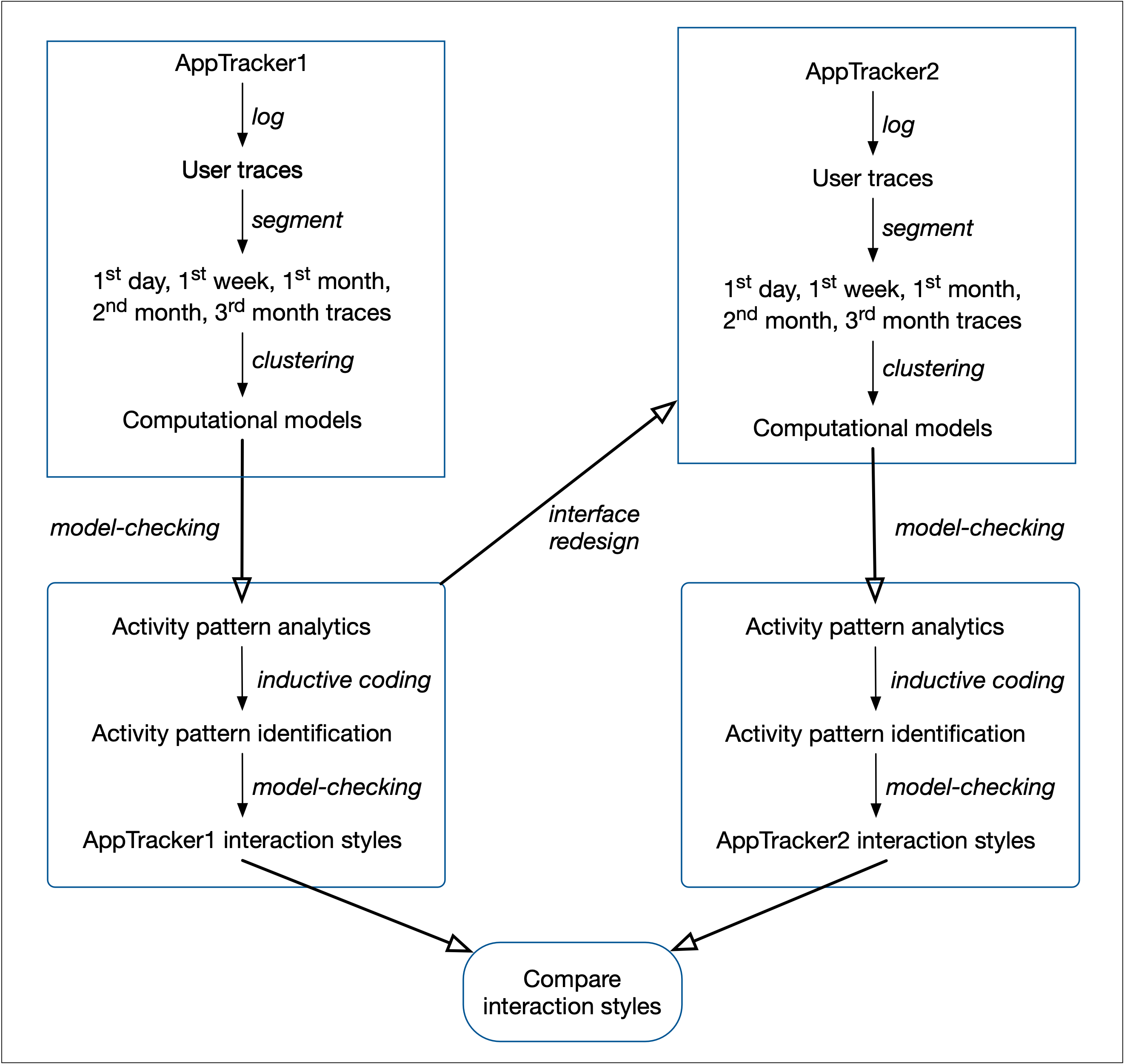
Figure 1: Study design

2.2 Time Series Data

Each logged user trace is a sequence of event labels. Each trace consists of many user interaction sessions, which start when the application is launched or being brought to the foreground (denoted by event startS) and end when the application is closed or put in the background (denoted by event stopS). User traces are segmented by time intervals $[t_{1},t_{2}]$ such that the first session of the segment occurs on or after time-stamp $t_{1}$ and the last session of the fragment occurs before time-stamp $t_{2}$; the whole trace may extend beyond time-stamp $t_{2}$.

2.3 Interface for AppTracker1

On launching AppTracker1, the main menu screen offers four main options (Fig. 2(a)); from top to bottom they are:

• Overall Usage contains summaries of all the data recorded since AppTracker1 was installed and opens the views OverallUsage and Stats (Fig. 2(b)).

• Last 7 Days opens the view Last7Days and displays a chart of activity of the user’s 5 most used apps during the last 7 days.

• Select by Period opens the view SelectPeriod and shows statistics for a selected period of time, e.g. which apps were used most since Friday, the daily time spent on Facebook over the last month, hourly device usage on Monday (Fig. 2(c)).

• Settings allows a user to start and stop the tracker, or to reset their recorded data.

There are 16 user-initiated events that switch between views (the name of the event is the resulting view), see state diagram in Fig. 3. States are grouped into Summary states for viewing summary or overall usage data; Specific states for viewing drilled down, specific data; Session-related states marking the start and the end of a session; and remaining states. Note state Last7Days is a summary state or a specific state depending on the context of use.

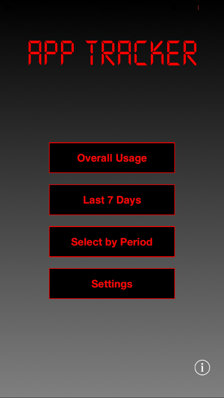
(a) Main menu

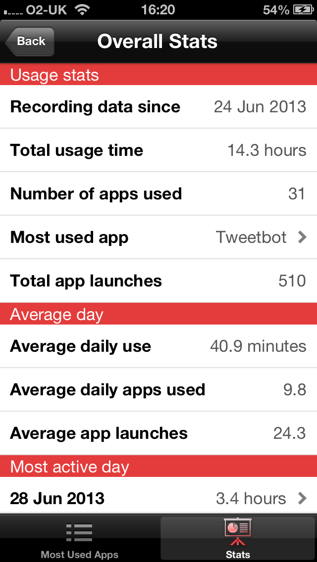
(b) Stats

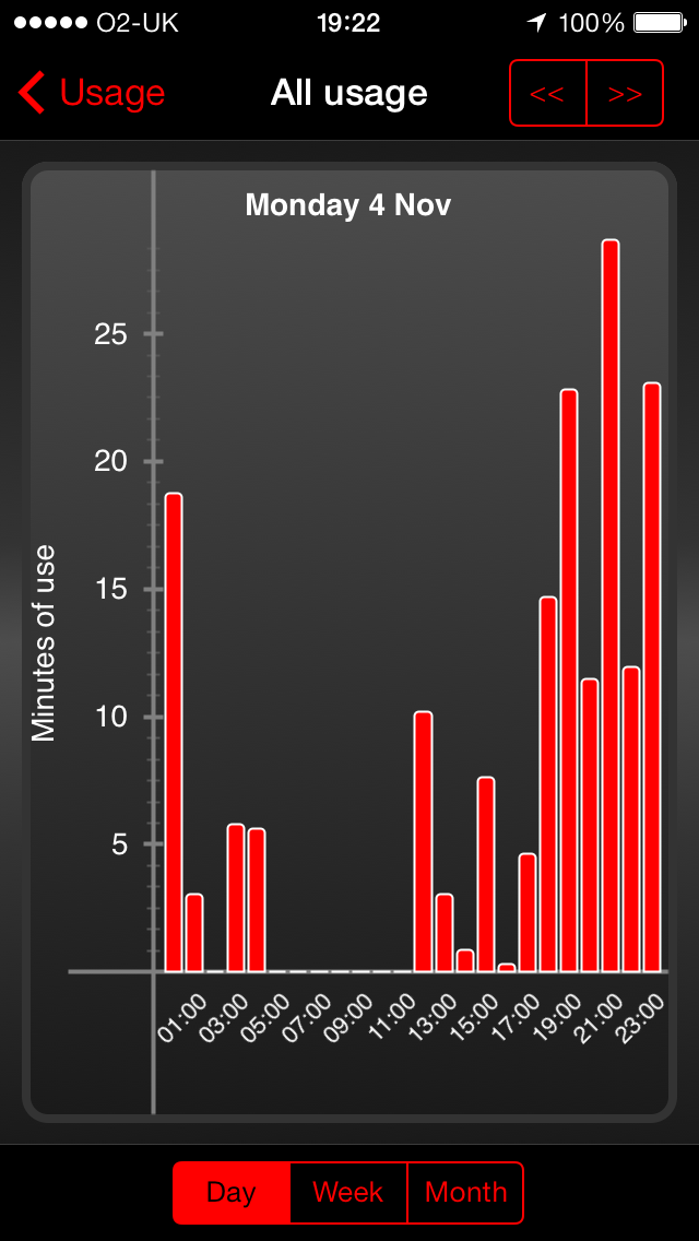
(c) Daily device usage

Figure 2: Screenshots from AppTracker1: (a) The main menu view corresponds to the state Main; (b) The stats view corresponds to the state Stats. (c) The daily device usage view corresponds to the state ChartOverall when the selected period is Monday 4 November.

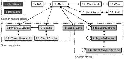
Figure 3: AppTracker1 state diagram. The vertical vertical layout of the menus corresponds to a left to right traversal of the states in the dotted boxes.

Logged interaction data are stored in a MySQL database using the SGLog framework [25] and processed using JavaScript to obtain user traces in JSON format. AppTracker1 was first released in August 2013 and downloaded over 35,000 times. Our data sets are taken from a sample of 322 user traces during 2013 and 2014. The maximum session count over all the traces is 129, the minimum was limited to 5.

2.4 Computational Methods

We used ML clustering methods to infer admixture Markov models, first defined in [1], based on first-order auto-regressive hidden Markov Models (AR-HMM) [38]. Admixture models permit interleaved variation, so we can model users that may switch interaction styles both within and between sessions. We include some definitions here for completeness.

A discrete-time Markov chain (DTMC) is a tuple $\mathcal{D}=(S,s_{0},\mathtt{P},\mathcal{L})$ where: $S$ is a set of states; $s_{0}\in S$ is the initial state; $\mathtt{P}:S\times S\rightarrow[0,1]$ is the transition probability function such that for all states $s\in S$ we have $\sum_{s^{\prime}\in S}\mathtt{P}(s,s^{\prime})=1$; and $\mathcal{L}:S\rightarrow 2^{\mathcal{A}}$ is a labelling function associating to each state $s$ in $S$ a set of valid atomic propositions from a set $\mathcal{A}$. A path (or execution) of a DTMC is a non-empty sequence $s_{0}s_{1}s_{2}\ldots$ where $s_{i}\in S$ and $\mathtt{P}(s_{i},s_{i+1})>0$ for all $i\geq 0$. A transition is also called a time-step.

A first-order auto-regressive hidden Markov Model (AR-HMM) [38] is as a tuple $(\mathcal{X},\mathcal{Y},\pi,A,B)$ where: $\mathcal{X}$ is the set of hidden (or latent) states $\mathcal{X}=\{1,\ldots,K\}$; $\mathcal{Y}$ is the set of observed states generated by hidden states; $\pi:\mathcal{X}\rightarrow[0,1]$ is an initial distribution with $\sum_{x\in\mathcal{X}}\pi(x)=1$; $A:\mathcal{X}\times\mathcal{X}\rightarrow[0,1]$ is the transition probability matrix, such that for all $x\in\mathcal{X}$ we have $\sum_{x^{\prime}\in\mathcal{X}}A(x,x^{\prime})=1$; $B:\mathcal{X}\times\mathcal{Y}\times\mathcal{Y}\rightarrow[0,1]$ is the observation probability matrix, such that for all $x\in\mathcal{X}$ and $y\in\mathcal{Y}$ we have $\sum_{y^{\prime}\in\mathcal{Y}}B(x,y,y^{\prime})=1$.

Now let $\mathcal{P}$ be a population of $M$ user traces over $n$ different types of event labels, $\mathcal{A}$ the set of the labels of all events occurring in $\mathcal{P}$, and $K$ a positive integer. A generalised population admixture model with $K$ components or GPAM($K$) for the user trace population $\mathcal{P}$ is a tuple $(\mathcal{X},\mathcal{Y},\pi,A,B,\mathcal{L})$ where $(\mathcal{X},\mathcal{Y},\pi,A,B)$ is an AR-HMM with $|\mathcal{X}|=K$ and $|\mathcal{Y}|=n$, and $\mathcal{L}:\mathcal{Y}\rightarrow{\mathcal{A}}$ is the labelling function mapping a unique event name to each observed state in $\mathcal{Y}$. A pictorial representation of a GPAM(2) is given in Fig. 4. For any GPAM $(\mathcal{X},\mathcal{Y},\pi,A,B,\mathcal{L})$ and a latent state $x\in\mathcal{X}$, the tuple $(\mathcal{Y},\mathcal{L}^{-1}(\texttt{startS}),B(x),\mathcal{L})$ is a discrete-time Markov chain (DTMC) called an activity pattern.

For each input data set $\mathcal{P}$ of user traces, we compute $n\times n$ transition-occurrence matrices for each trace $\alpha$ such that matrix position $(i,j)$ is the number of times the subsequence $\alpha_{i}\alpha_{j}$ (i.e. two adjacent event labels) occurs in $\alpha$. The resulting transition-occurrence matrices are the input data for ML; we employ the Baum—Welch clustering algorithm [49], which uses the local non-linear optimisation Expectation–Maximisation (EM) algorithm [17] for finding maximum likelihood parameters of observing each trace, and restarting the algorithm whenever the log-likelihood has multiple-local maxima.

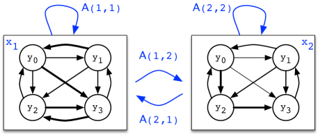
Figure 4: Pictorial representation of a GPAM(2) with the latent states $x_{1}$ and $x_{2}$. The two activity patterns are the DTMCs in each box; there are four observed states $y_{0},y_{1},y_{2},y_{3}$. Transition probabilities are indicated by the thickness of transitions.

We used the probabilistic model checker PRISM [31] to analyse temporal properties expressed in rPCTL, an extension of Probabilistic Computation Tree Logic PCTL* [31, 5] with rewards; an overview can be found in Appendix 0.B.

The set of parameterised properties we defined and used is contained in Table 1. These temporal properties express behaviour within an activity pattern or behaviour that involves several activity patterns. The properties of the latter type are StateToPattern and LongRunPattern, and we used them for model checking on GPAMs only. The rest of the properties were used on activity patterns as DTMCs. First we model-check the temporal properties VisitProbInit, StepCountInit, VisitCountInit, SessionLength, and SessionCount for different, incremental values of $K$ for all states. Optionally, we use the properties VisitProbBtw and StepCountBtw when it is too difficult to interpret the results from the other properties on activity patterns. Then the properties StateToPattern and LongRunPattern help us identify more nuanced characteristics by considering if an activity pattern changes within a session and the long run probability of each activity pattern, respectively. Other PTCL* properties considered, but not included in this paper, helped us analyse whether some particular states lead to the end of a session in fewer steps than other states and whether there are correlations between state formulae (over states and/or patterns).

Table 1: Reward-based PCTL (rPCTL) properties are parameterised by: $N$ a positive integer value for the number of time steps; $j,j_{1},j_{2}$ positive integer values denoting observed state identifiers; $i,i_{1},i_{2}$ integer values between 1 and $K$ denoting the hidden state identifiers (activity patterns); $p\in[0,1]$ a probability.

Name	Formula and informal description
VisitProbInit	$\mathtt{P}_{=?}[\mathtt{true}\,{\sf U}^{\leq N}(y=j)]$ : probability to reach $j$ from the initial state within $N$ steps
StepCountInit	$\mathtt{R}_{\texttt{rSteps}=?}[{\sf F}\,(y=j)]$ : expected number of steps to reach $j$ from the initial state
VisitCountInit	$\mathtt{R}_{\texttt{rStatej}=?}[{\sf C}^{\leq N}]$ : expected number of visits to $j$ within $N$ steps
SessionLength	$\mathtt{R}_{\texttt{rSteps}=?}[{\sf F}\,(y=\texttt{stopS})]$ : expected number of steps until the end of session.
SessionCount	$\mathtt{R}_{\texttt{rState{stopS}}=?}[{\sf C}^{\leq N}]$ : expected number of sessions within $N$ steps
VisitProbBtw	$\mathit{filter}(\mathsf{state},\mathtt{P}_{=?}[(\lnot\texttt{stopS})\,{\sf U}^{\leq N}(y=j_{2})],(y=j_{1}))$ : probability of reaching observed state $j_{2}$ from $j_{1}$ within the same session
StepCountBtw	$\mathit{filter}(\mathsf{state},\mathtt{R}_{\texttt{rSteps}=?}[{\sf F}\,(y=j_{2})],(y=j_{1}))$ : expected number of steps to reach state $j_{2}$ from $j_{1}$
StateToPattern	$\mathtt{P}_{\geq 1}[\,{\sf F}\,(x=i_{1}\land y=j)]\land\mathtt{P}_{\geq 1}[\,{\sf G}\,((x=i_{1}\land y=j)\Rightarrow\mathtt{P}_{>p}[(x=i_{1}\land\lnot\texttt{stopS})\,{\sf U}\,(x=i_{2})])]$: likelihood of observed state $j$ in activity pattern $i_{1}$ leading to changing the activity pattern to $i_{2}$ within the same session
StateToStop	$\mathtt{P}_{\geq 1}[\,{\sf F}\,(x=i\land y=j)]\land\mathtt{P}_{\geq 1}[\,{\sf G}\,((x=i\land y=j)\Rightarrow\mathtt{P}_{>p}[(x=i)\,{\sf U}\,\texttt{stopS}\,])]$ : likelihood of observed state $j$ in activity pattern $i$ leading to the end of a session, without changing the activity pattern
LongRunPattern	$\mathtt{S}_{=?}[\,x=i\,]$ : probability of being in activity pattern $i$ in the long run

Observed states are grouped, according to their expected function and purpose within the application, for example Summary and Specific for AppTracker1. This grouping is done iteratively: an initial grouping is proposed by the designers, then after analysing the results of the temporal properties within each activity pattern, the analysts and designers may, together, revise the grouping. Note that such state groups may overlap.

The source code for the quantitative analysis is available online .

2.5 Inductive Coding

While the PRISM model checking results are quantitative, interpretation of those results is subjective, and therefore similar to the interpretation of qualitative data. We adopt the general inductive approach for analysing qualitative evaluation data [46] that aims to allow research findings to emerge from the data, rather than a deductive approach that tests a hypothesis.

Coding was carried out independently by two evaluators (authors Andrei and Calder), with several revisions and refinements, then checked for clarity (all four authors), and stakeholder checks (Morrison and Chalmers as designers). We note that many hours were spent choosing meaningful labels. Since the labels themselves have inherent meaning, the labels were changed several times throughout this work, as we gained a deeper understanding of all the nuances of the activity patterns. We suggest this is both a strength and a weakness of our approach.

3 Study Results

We give an overview of results, following the study flow in Fig. 1. For brevity we report results only for GPAM(2) models; details for GPAM(3) models are available in Appendix 0.C. We refer to results for models from data sets for 1st day, 1st week, and 1st month as results for early days usage and for the 2nd and 3rd month as experienced usage.

For inferring the models, Baum-Welch algorithm was implemented in Java and ran on a 2.8GHz Intel Xeon (single thread, one core); it was restarted 200 times with 100 maximum number of iterations for each restart. As example performance, for the data set consisting of the first month of usage, the algorithm took 3.2 min for $K=2$, 4.1 min for $K=3$, and 5.3 min for $K=4$.

We started by model checking the properties VisitProbInit, StepCountInit, VisitCountInit, SessionLength, and SessionCount for $K=2$ for all states. We selected a single value for $N$, typically somewhere between $10$ and $150$; in our experience $50$ is a good starting value. Note that the result from the model checker may not be a number (either probability or positive real), due to state unreachability, a filter satisfying no states, or the iterative method not converging within 100,000 iterations (limit chosen for the PRISM model checker). In this case the result is given as ”—”. To aid interpretation, results are ordered ”best” to ”worst” as follows: greatest to least value for VisitProbInit, VisitProbBtw, and VisitCountInit, while least to greatest value for StepCountInit and StepCountBtw. This ordering reflects the following judgments: a higher probability to visit a state, a higher number of state visits, and fewer steps to reach a state, are all indicators of greater (user) interest in a state or a pair of states. We encode this ordering visually using the colour blue for the ”best” results and purple for the ”worst” results.

3.1 AppTracker1 Interaction Styles

Tables 2 and 3 include activity pattern results for the temporal properties VisitProbInit, VisitCountInit, and StepCountInit analysed on GPAM(2) models inferred from different time intervals of usage.

We say that a state is predominant within an activity pattern if: (i) the probability to reach it computed using VisitProbInit is greater than 0.5, the visit count computed by VisitCountInit is greater than 1, and the number of time steps to reach it computed by StepCountInit is lower than the time bound $N=50$ chosen for the temporal properties, and (ii) there is no other activity pattern in the same model where the VisitCountInit and StepCountInit score at least three times better. An activity pattern is centred on a set of states (or state grouping they belong to) when those states are predominant within the activity pattern. Activity patterns are labelled according to two dimensions: usage intensity and predominant states. Values in a usage intensity type are based on abstractions of the frequency and length of session, as well as on results returned by the properties VisitProbInit, VisitCountInit, StepCountInit, VisitProbBtw, and StepCountBtw for the predominant states in relation to the intensity usage type.

Table 4 shows our workings through the inductive coding process:

• First we consider session characteristics and use the Jenks natural breaks optimisation method [28] to determine the best arrangement of session count values into three categories, and similarly for the session length.

• Second, we give an initial categorisation of the activity patterns based on session characteristics and predominant states. We can see immediately there is a correlation between fewer/longer sessions, and more numerous/shorter sessions. We note that more many/long sessions and few/short sessions did not occur. The state identifiers upon which each activity pattern is centred are listed in decreasing order of their results: the better the result for a state in a pattern (the higher probability to reach, the higher visit count, the fewer steps to reach) the higher the predominance of that particular state compared to other states. We refer to a subset of states as TopLevelMenu, these are states that are reached in one or two button presses in average (corresponding to time steps in the respective DTMC).

• Third, we conclude that the usage intensity type consists of three values that we call Browsing, Glancing, and Focussing.

• Finally, we combine usage intensity and predominant state group type to assign four activity pattern labels. Note that two possible combinations are not present: GlancingSummary and BrowsingSpecific.

We can see a clear split between the activity patterns for early days usage and experienced usage.

After labelling of the activity pattern, a further analysis based on model checking is carried out to investigate further the relationships between them using the temporal properties LongRunPattern and StateToPattern, hence find out more about the interaction styles. The long run probabilities for activity patterns are shown in Fig. 10(a) and probabilities that, for a given activity pattern, a state leads to activity pattern change (within a session) are given in Fig. 6(a). The latter shows that for the early days usage, all states are highly likely (close to probability 1) to transition from GlancingSpecific to BrowsingSummary behaviour, and less likely the other way around (probability between 0.5 and 0.75), except for Stats for which the probability is around 0.2, and for ChartOverall and ChartAppsInPeriod with even lower probability. These two exceptions correlate with the results highlighted in the StateToStop analysis (not shown here) that indicate that once in BrowsingSummary in any of the states Stats, ChartOverall, and ChartAppsInPeriod, it is unlikely to move to another activity pattern before the end of session. In the experienced user models, it is more likely to move from FocussingSummary to FocussingSpecific than the other way around, but overall, it is unlikely to move between these two patterns within a session.

In conclusion, the interaction styles of AppTracker1 based on GPAM(2) models are summarised as follows. Early days usage contained Glancing and Browsing patterns, the latter possibly because users explore all the screens and features offered by the app. For experienced users, usage is focussed with FocussingSpecific being a little more likely. Glancing patterns involve the shortest sessions in terms of screen view counts over all patterns, and also appear as the most numerous sessions. We note similarity in these Glancing patterns to the micro-usages discussed in [22], defined as ”brief bursts of interaction with applications”.

Table 2: AppTracker1 activity pattern analytics. Results for the properties VisitProbInit, VisitCountInit, and StepCountInit instantiated with $N=50$, the states OverallUsage, Last7Days, SelectPeriod, Stats, AppsInPeriod, and the two activity patterns, which we call AP1 and AP2, on GPAM(2) models for five time intervals. Each row corresponds to a GPAM(2) model learned from the segmented data set for the respective time interval. Blue indicates best result and purple indicates worst for a particular state across the activity patterns in a GPAM(2) model for a particular time interval.

Prop.	Time	OverallUsage		Last7Days		SelectPeriod		Stats		AppsInPeriod
	interval	AP1	AP2	AP1	AP2	AP1	AP2	AP1	AP2	AP1	AP2
VisitProbInit	[0,1]	0.94	0.99	0.80	0.89	0.80	0.42	0.81	0.99	0.45	0.13
	[0,7]	0.67	0.99	0.89	0.88	0.88	0.48	0.55	0.99	0.67	0.21
	[0,30]	0.59	0.99	0.91	0.92	0.90	0.56	0.46	0.98	0.76	0.29
	[30,60]	0.87	0.99	0.98	0.31	0.93	0.00	0.45	0.96	0.77	0.00
	[60,90]	0.91	0.99	0.97	0.02	0.96	0.10	0.56	0.91	0.83	0.09
VisitCountInit	[0,1]	3.54	14.58	1.63	2.24	1.92	0.72	1.74	5.77	0.95	0.28
	[0,7]	1.19	15.25	2.21	2.09	2.75	0.87	0.84	5.27	2.11	0.48
	[0,30]	0.89	15.55	2.39	2.52	2.62	1.19	0.65	4.75	1.95	0.69
	[30,60]	2.28	14.27	5.06	0.40	4.29	0.01	0.80	4.04	4.39	0.01
	[60,90]	3.00	14.73	4.48	0.02	4.61	0.10	1.28	3.63	5.64	0.82
StepCountInit	[0,1]	16.55	4.53	30.27	22.75	30.45	90.36	29.82	12.01	83.40	332.40
	[0,7]	44.55	3.63	22.14	23.24	23.27	75.96	63.24	12.58	45.55	210.12
	[0,30]	56.55	3.44	20.07	19.28	21.53	59.94	81.13	13.68	35.54	145.35
	[30,60]	23.41	2.15	9.02	137.09	18.90	5483.99	85.45	15.97	34.45	25915.18
	[60,90]	19.55	2.23	10.46	2269.78	15.49	483.09	61.19	21.01	28.65	532.74

Table 3: AppTracker1. Characteristics of sessions in GPAM(2): VisitProbInit for the state UseStop computes the probability to reach the end of the session, while SessionCount and SessionLength compute the expected number of sessions and the expected number of time steps (button taps) in a session respectively.

Time	VisitProbInit		SessionCount		SessionLength
interval	AP1	AP2	AP1	AP2	AP1	AP2
$[0,1]$	0.99	0.31	10.13	0.37	3.86	130.96
$[0,7]$	0.99	0.43	10.20	0.54	3.81	87.76
$[0,30]$	0.99	0.38	10.82	0.47	3.51	102.07
$[30,60]$	0.99	0.99	6.17	7.55	7.09	5.36
$[60,90]$	0.99	0.99	5.43	7.35	8.28	5.56

Table 4: AppTracker1. GPAM(2). Inductive coding: categorisation of the average session counts and lengths, subsequently used for the initial categorisation of activity patterns alongside the predominant states, and description of the usage intensities. State identifiers (ids) are: 3 is OverallUsage, 4 is Last7Days, 5 is SelectPeriod, 6 is AppsInPeriod, 9 is Stats, 10 is ChartOverall, 12 is ChartStats, and 14 is ChartAppsInPeriod. State identifiers are highlighted as Summary states and Specific states. State 4 has a dual role as Summary or Specific depending on the context.

Categories of session counts few mid many $\{0.37,0.47,0.54\}$ $\{5.43,6.17,7.35,7.55\}$ $\{10.13,10.82\}$

Categories of session lengths short mid long $\{3.51,3.81,3.86\}$ $\{5.36,5.56,7.09,8.28\}$ $\{87.76,102.07,130.96\}$

Time AP1 AP2 interval Sessions Predominant Session Predominant characteristics states characteristics states $[0,1]$ many/short 5,9,4 few/long 3,9,4,10,12 $[0,7]$ many/short 5,4,6 few/long 3,9,4 $[0,30]$ many/short 5,4,6 few/long 3,9,4,12 $[30,60]$ mid/mid 4,5,6,14 mid/mid 3,9,10,12 $[60,90]$ mid/mid 6,5,4,14 mid/mid 3,10,9,12

Usage intensity Usage intensity characteristics Browsing few/long sessions centred on at least three states in the TopLevelMenu, sometimes from different state groups Glancing many/short sessions centred on one or two states Focussing mid/mid sessions centred on states from the same group

Time interval		AP1 label	AP2 label
$[0,1]$		GlancingSpecific	BrowsingSummary
$[0,7]$		GlancingSpecific	BrowsingSummary
$[0,30]$		GlancingSpecific	BrowsingSummary
$[30,60]$		FocussingSpecific	FocussingSummary
$[60,90]$		FocussingSpecific	FocussingSummary

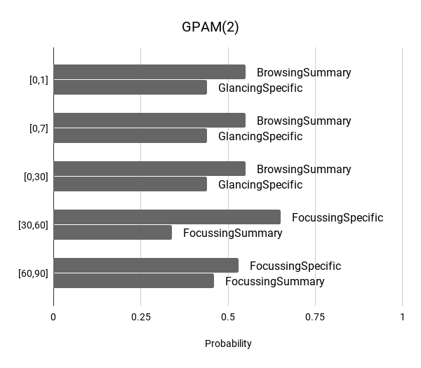
(a) AppTracker1

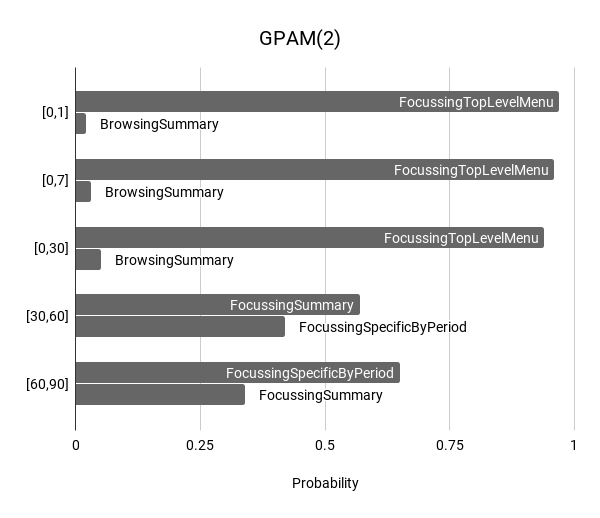
(b) AppTracker2

Figure 5: AppTracker1 and AppTracker2. Visualisation of probabilities of being in each activity pattern in the long run in GPAM(2) models for different time intervals; the entries are ordered decreasingly for each time interval. These results are based on model checking the temporal property LongRunPattern for each activity pattern.

(a) AppTracker1

(b) AppTracker2

Figure 6: AppTracker1 and AppTracker2. Visualisations of the average likelihood of changing activity pattern from an state within a session in GPAM(2) models for different time intervals. Excepting the Stats and ChartStats states, for which the property returns lower probabilities than the average, the probabilities returned for all states are very similar. Dotted arrows denote probabilities in $[0.02,0.2)$, thin arrows in $[0.5,0.8)$, and thick arrows $\geq 0.8$. Likelihoods lower than 0.02 are omitted. These results are based on model checking the temporal property StateToPattern for various combinations of states and activity patterns.

An important question to ask is: does the latent structure we uncover simply reflect the top level menu structure? To answer it we looked at GPAM(3) models (see Appendix 0.C), since there are three main menu options (excluding Settings). If the activity patterns simply reflect the menu structure, then when we would expect each of the patterns in GPAM(3) to be centred on one the above states, with very low correlations between pairs of those states. This was not the case. In all five GPAM(3) models we found activity patterns with either Focussing or Glancing usage intensity, centred around Last7Days and either SelectPeriod or AppsInPeriod; there was no model with one pattern centred on either SelectPeriod or AppsInPeriod but no Last7Days  and another pattern centred on Last7Days, but not on SelectPeriod or AppsInPeriod.

3.2 Redesigning the Interface for Experienced Usage

It became evident that AppTracker1’s top-level menu was not a good fit for users’ interaction styles. For example, we uncovered Glancing behaviours, where users would quickly consult the app to view their usage behaviour, but this did not fit well with the menu structure: a user could glance at all-time most-used apps (OverallUsage state) within the first menu item, but if they had used AppTracker1 for a long time, it becomes increasingly likely that this list would be static. Conversely, while a user could find recent (e.g. today’s) usage, this would involve several steps through the menu of more detailed information.

We chose to concentrate on redesign for experienced usage; these were users who had voluntarily continued with the app over a period of time so we also expected to see more stable interaction styles, where initial user learning processes have subsided. An equally valid alternative would have been early stage users, for example to work on issues that may improve retention of users beyond the initial experiences.

Our aim was not to change the overall purpose of AppTracker, or to add new features, but to reconfigure the menu structure, by adding, removing or moving states, to increase the support for more efficient Glancing on Summary states and Focussing on Specific states. These behaviours were not well aligned with the existing menu layout. For example, we see AppsInPeriod (from the Specific sub-menu) appear in Glancing activity patterns, because users might drill down into the specific menus to see the current day’s activity. Table 4 also shows activity clustering around Summary and Specific states during experienced usage, but not in an efficient way; users are seen to be Focussing on Summary states, when such information could be presented in such a way as to allow glancing to acquire the desired information more quickly.

As a consequence we changed the top level menu structure to offer two options (plus Settings) instead of three. The two options correspond to Glancing and Browsing usage, and to Focussing usage, and we call them My Top Apps and Explore Data, respectively. The corresponding two state groups are Summary states and Specific states (as the union of SpecificMenu, SpecificByPeriod, SpecificByApp, and SpecificStats state groups). Hence, several states further down the hierarchy are moved or split, i.e. moving states upon which an activity pattern is centred to be close to the option associated with that activity pattern. To support Glancing and Browsing usage behaviour, My Top Apps contains only tables showing: (i) the user’s most-used apps since installation of AppTracker and (ii) the most-used apps on the current day. This way the redesigned menu aims to make today’s usage much more easily accessible from the top-level menu.

The changes are illustrated in Fig. 8 and summarised as:

• The app’s menu is restructured to specifically support as two main styles of use Glancing and Focussing, and therefore to only have two main menu options to make these behaviours more distinct.

• The screen view OverallUsage was replaced by a new, more glancing-like view OverallAll  that does not allow for drilling down into detailed usage.

• A new glancing-like screen view AppsToday is included in the Summary part of the menu.

• The screen view Last7Days was removed.

• The Specific states group of the menu was broken up into more subtle sub-components: SpecificByPeriod, SpecificByApp, SpecificStats.

• The screen view OverallUsage was moved into the Specific part and renamed as OverallbyApp alongside with ChartOverallbyApp; these two new states are grouped into SpecificByApp.

• The screen view Stats was moved into the Specific part of the menu alongside with ChartStats; these two new states are grouped into SpecificStats.

The main menu screen of AppTracker2 offers three main options (Fig. 7(a)), and there are 18 user-initiated events. New states are:

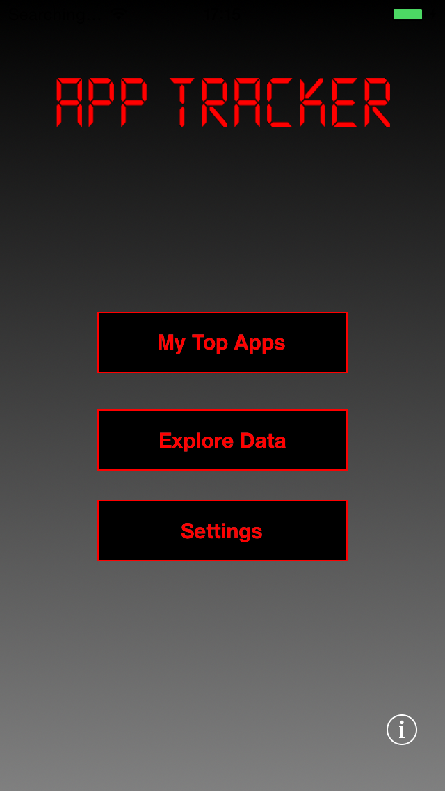
(a) Main Menu View

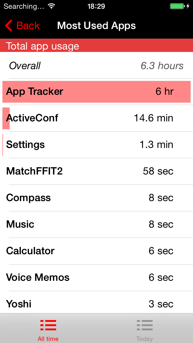
(b) My Top Apps Sub-menu

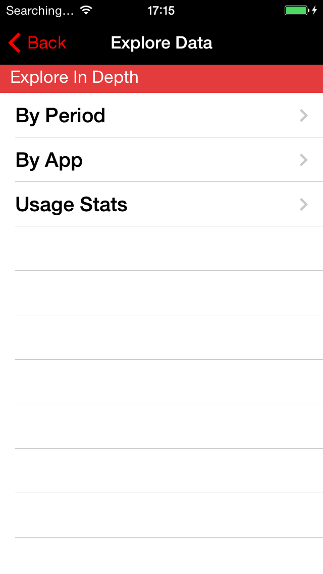
(c) Explore Data Sub-menu

Figure 7: Screenshots from AppTracker2: (a) The main menu view corresponds to the state Main; the My Top Apps option takes the user to the state OverallAll, Explore Data to the state ExploreData, and Settings to the state Settings. (b) The My Top Apps view (corresponding to the state OverallAll) shows the overall usage of the device since installing the app and offers the possibility to view today’s usage – the bottom-right option Today. (c) The Explore Data view offers the options of exploring the data By Period (state SelectPeriod), By App (state OverallbyApp), and viewing the Usage Stats (state Stats).

• OverallAll: summary statistics about the overall device usage since installing AppTracker2,

• ExploreData: three options for more in-depth exploration of all recorded data,

• AppsToday: summaries of the current day’s usage of apps,

• AppsbyPeriod: usage statistics for various apps by selected time period,

• ChartAppsInPeriod: detailed app usage when selected from AppsbyPeriod,

• OverallbyApp: usage summary for a selected app,

• ChartOverallbyApp: detailed app usage, when selected from OverallbyApp.

States are grouped, depending on position in the overall AppTracker2 menu, insights gained from the interaction styles of AppTracker1, and design intentions of AppTracker2. AppTracker2 was released in 2016 and our data sets are taken from a sample of 600 user traces over a period of six months.

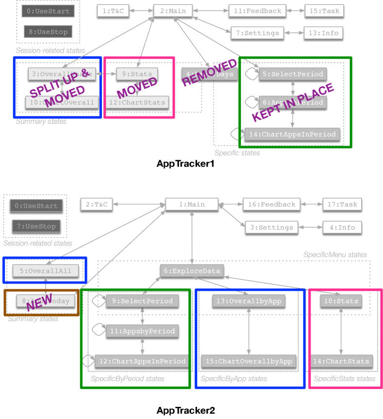
Figure 8: AppTracker1 and AppTracker1 interface designs. We use same colours between the two app versions to show correspondence.

3.3 AppTracker2 Interaction Styles

For brevity we show only our working for the inductive coding process for GPAM(2) models in Table 5. The labels are self-explanatory, but it is important to note that Summary states are a different grouping than in AppTracker1, see Fig. 8. In particular the new state AppsToday (state 8) features in all the activity patterns except FocussingSpecificByPeriod. The main result is again there are four distinct activity patterns and a clear split between styles for early days usage and experienced usage. Long run probabilities are in Fig. 10(b) and probabilities that for a given activity pattern, a state leads to activity pattern change (within a session), are given in Fig. 6(b).

The interaction styles for GPAM(2) models of AppTracker2 usage are summarised as follows. Overall, there are fewer and shorter sessions, there are no short sessions and no mid/mid combinations. There is much more Focussing  behaviour. There is very little Browsing in the early days models, which could indicate that AppTracker2 is easy to use, or that most of the users are already experts in using this second version of the app. The probabilities to transition are low across all models.

Table 5: AppTracker2, GPAM(2) models. Categorisation of the average session counts and lengths, subsequently used for the initial categorisation of activity patterns alongside the predominant states, and description of the usage intensity labels. State identifiers (ids) are: 5 is OverallAll, 6 is ExploreData, 8 is AppsToday, 9 is SelectPeriod, 10 is Stats, 11 is AppsbyPeriod, 12 is ChartAppsInPeriod, 13 is OverallbyApp, 14 is ChartStats, 15 is ChartOverallbyApp. State identifiers are highlighted as Summary states and Specific states.

Categories of session counts few many $\{1.40,2.10,3.04\}$ $\{5.35,5.86,5.87,6.23,6.39,6.52,7.02\}$

Categories of session lengths mid long $\{6.14,6.57,6.68,6.88,7.52,7.84,8.31\}$ $\{17.61,25.08,38.84\}$

Time AP1 AP2 int. Sessions States ids Sessions States ids $[0,1]$ few/long 5, 8,6 many/mid 5,6,8,9 $[0,7]$ few/long 5, 8,6 many/mid 5,6,8,9 $[0,30]$ few/long 5,6,8 many/mid 5,6,8,9 $[30,60]$ many/mid 9, 6, 11, 12 many/mid 5, 8, 6,6 $[60,90]$ many/mid 6, 9, 11, 12 many/mid 5, 8,6

Usage intensity Usage intensity characteristics Browsing few/long sessions centred on at least three states in the TopLevelMenu, sometimes from different state groups Focussing many/mid sessions centred on states from the same group

Time int. AP1 label AP2 label $[0,1]$ BrowsingSummary FocussingTopLevelMenu $[0,7]$ BrowsingSummary FocussingTopLevelMenu $[0,30]$ BrowsingSummary FocussingTopLevelMenu $[30,60]$ FocussingSpecificByPeriod FocussingSummary $[60,90]$ FocussingSpecificByPeriod FocussingSummary

3.4 Comparing Interaction Styles in AppTracker1 and AppTracker2

Comparing the interaction styles in AppTracker2 with AppTracker1, there are many similarities between activity patterns, and these are reflected in the label names. This is not surprising, given the redesign involved menu re-organisation, not a full-scale application redesign. The major differences between the styles can be seen in Fig. 5 and Fig. 6. We summarise the effects of the redesign on interaction styles as: AppTracker2 has no short sessions, more Focussing in all models, with Focussing on specific states more likely for experienced users, very little Browsing, and with low likelihood, and only in early days usage models, extensive occurrences of the new summary state AppsToday, and a lower likelihood to move out of an activity pattern. The last may indicate more alignment with user intention and in particular with experienced user, or that most of the users are already experts in using this second version of the app. One could argue that the FocussingTopLevelMenu observed in the early days usage is a form of longer, but focussed Glancing. It is interesting to note that while the redesign was targeted mainly at experienced users, it had a significant, positive effect on early days users.

3.5 Insights from Models with at Least Three Clusters

Increasing the number of clusters $K$ to $3$ revealed more fine-grained interest in selected states or sets of states, and also the possibility of very short sessions in AppTracker2. For example, in GPAM(3) we uncovered Glancing  again for experienced usage, but it was entirely focussed on the Main menu or on the (new) Summary states. A brief analysis of GPAM(3) models for both AppTracker1 and AppTracker2 can be found in the Appendix 0.C.

We observed that as we increase the number of model components, we see some finer-grained interest in selected states or groups of states (e.g. in FocussingSpecific in GPAM(4) and GPAM(5) models) that was less prominent for smaller values of $K$. For $K\geq 4$ we see more activity patterns that are centred around each of the states. There is no optimal value for $K$, in general. It is an exploratory tool whose usefulness depends on the number of state groups, the state diagram, and the granularity that is helpful for redesign. In this study we found 2-3 clusters most useful. Note, we needed to study at least $K=3$ to investigate whether activity patterns align to top level menu choices. It was also important to analyse GPAM(4) and GPAM(5) models to confirm they did not reveal significantly different or more useful (for redesign) activity patterns; details of GPAM(4) and GPAM(5) analyses are not included here.

4 Discussion

We reflect on some implications of working with data-driven ML models and computational methods.

4.1 Data Reliability and Segmentation

We identified and subsequently fixed several errors in the logs such as missing start or end of sessions, missing events, unexpected timestamps, all due to the interactions between the logging framework SGLog and iOS such as apps crashing before data were written to file, or network failures in transmitting data to our servers for analysis. We discarded the user traces with less than five sessions because our focus was on studying long term engagement and such short user traces would only add more noise in the data set. The choice of five sessions as cut off for the minimum user trace length was empirical and we cannot exclude that a different minimum would produce different results.

We selected different time intervals that covered experiences from initial engagement (first day) to extended engagement (over several months). These intervals were of interest, and made sense to us, for this application. More generally, designers might choose to focus on different intervals, at different times. For example, shortly after release of an initial design, they may focus on models inferred from first day usage (or even shorter, e.g. the first five minutes), but in subsequent designs they may choose to consider only models inferred from usage data from users that engage for long periods of time.

4.2 Bias in Data Sets

AppTracker2 was released as an update to AppTracker1 (both available only on the Cydia app store for jailbroken iOS devices). As such, our set of AppTracker2 users could be either existing users who installed the update, or new users coming to the app afresh. This might have an effect on interaction styles, because existing users would be more familiar with the system, and would also have existing logged information recorded, so would be looking at charts and tables already populated with data, whereas new users would see empty screens during the early days. More generally, it can be a challenge to distinguish new users, because users can reinstall an app or purchase new hardware. For example, Apple altered the type of unique device identifiers that apps can access, to track users across installations. More recently Apple have prohibited this entirely, such that if a user uninstalls all apps from a developer and then re-installs, an entirely new identifier is generated, and nothing is provided that can link the user of the second installation to the first one (and vice versa) [9, 40]. These are issues inherent in performing real world deployments of apps rather than conducting more constrained lab-style research. We would argue that great benefits are gained from the large number of users we were able to recruit, and the external validity gained through users ‘self-selecting’ to download our app rather than having being explicitly recruited as participants in a trial, and our subsequent study of people’s use of our apps on their own devices embedded in their everyday lives.

4.3 Selection of States, Volume of Data, and Scalability

Our study gained from having significant volume of log data to work on, for reliable application of ML methods. It is important to note that neither the volume of log data nor number of user traces is relevant to probabilistic model checking; only the number of observed states determines its complexity. The AppTracker study involved a vocabulary of 16-18 observed states, which was comfortably manageable, but model-checking would have difficulty with an order of magnitude larger. This could arise in an app with much richer menu options, or further inclusion of categorical variables such as location, demographic information, duration of the event, time of day or week, etc.

4.4 User Proficiency and Focus over Time

Simpler forms of analytics may chase absolute metrics such as spending longer in the app or launching the app more often as measures of engagement [4]. We did we not conflate (subject) intensity of usage with usage expertise and/or proficiency. We aimed to support the styles that were observed, and note that both Focussing and Glancing styles were present in experienced usage models.

4.5 Further Redesign Possibilities

New users. If there is a difference between new and longer-term users (e.g. first day/week/month users vs. second/third month users), then add new functionality that supports application ‘onboarding’ and a smooth transition into another style of interaction.

Micro-usages. Look for activity carried out in very brief micro-usages that might be better served by widgets rather than navigating the full application. By widget we mean a simple additional element of a device’s graphical interface, which is usually complementary to an application running on that device.

Shortcuts. Identify the most popular initial states in an activity pattern and implement shortcuts to these states.

Split the application. If there is (nearly) always only one activity pattern per session and patterns do not overlap, then split the application into two (or more) separate applications.

5 Related work

5.1 Our Previous Work

We developed our analytics over a number of years: refining the Markovian models, the temporal properties, and segmentation of data sets. Our first study [3] involved the iOS multi-player game Hungry Yoshi [35], one data set, a simple inferred model, simple temporal logic properties, and $K=2$. The app was different to AppTracker in that it had clear (user) goal states and (in addition to user interactions) external events when the device picked up scanned Wi-Fi access points. We uncovered two interaction styles representing different strategies for playing the game, but could not implement a redesign because Apple’s iOS changes meant we could no longer scan for Wi-Fi access points. The app is no longer under development. Our initial analysis of AppTracker [2] used a different inferred admixture model, a restricted set of generic temporal properties, and segmented data sets. There was no inductive coding nor menu redesign. The GPAM model was defined in [1], where we also introduced the possibility of logic formulae over the latent variables, though we did not consider the probability to transition between activity patterns. Significantly, none of our earlier work involved specific design recommendations, the implementation and deployment of a new design, nor analysis of interaction styles in the new design.

5.2 Other Related Work

Our approach to modelling was motivated initially by an empirical study of simplicial mixtures for modelling webpage browsing and telephone usage [24]. We note that in the same year, Bowring et al. [11] referred to Girolami et al.’s work [24] when suggesting that a hidden Markov model for automatic classification of software was possible future work. To our knowledge, no one else has investigated admixture models for modelling interaction behaviour, however the existence of different user-populations or user types among the larger mobile app user population was also recently highlighted in [15, 29, 52] and mixture models proposed.

Markov chains as models for software usage were proposed nearly 30 years ago by Whittaker and Poore [50], where transition probabilities are estimated from the frequency counts of all bigrams occurring in the execution traces. We can consider this model as a GPAM with only one component, i.e. GPAM(1). Markov chain models of software behaviour have also been employed in [16, 45] and more recently in [23, 12, 34, 30, 48, 20]. Usage styles are uncovered using statistical methods in [30], though not as latent states in a hidden Markov model variant. The analysis techniques used in [50] or in [45] are classic mathematical operations on the transition matrix such as computing the long run probability of being in one state or the expected number of states transitions to first reach a state (mean first passage time), whereas we use probabilistic temporal logic properties, which allows for more expressive properties to be formulated and then analysed automatically in a probabilistic model checking tool. First-order Markov models have been used for modelling in many related problems such as: human navigation on the Web, where states correspond to visited webpages [10, 14, 42, 41, 23], more specifically clickstream data [36, 33, 8], usability analysis, where states correspond to button presses in general [45], mobile applications, where states correspond to device screen events [3, 30], and human interactions with a search engine [47].

Research on mobile app usage by Banovic et al. [6] presents evidence for (and characterises sessions based on) duration and interaction types such as glance, review and engage. We also identified three types of usage intensity (Glancing, Browsing and Focussing), however they are characterised by the number of in-session interactions and frequency of sessions. We note that both our Glancing and the glance of [6] involve micro-usages. We suggest our characterisation of glancing behaviour is closer to that of checking habit [39] as brief, repetitive inspection of dynamic content quickly accessible on the device. The BEAR tool [23] is similar in that it infers discrete time Markov chains from logs and probabilistic temporal logic properties and PRISM are used to query the models; but the key difference is users are classified according to static attributes, e.g. by time zone or operating system, which the designer has pre-defined, and behaviours are assumed to be homogeneous, i.e. there is no in-class variation and no ability to express or detect hybrid behaviours. This issue is also raised in [12], arguing that the filters for partitioning the log data can have a dramatic effect on the resulting model and the subsequent analyses.

We also note DTMCs are models for usage patterns in [43], where mHealth apps are analysed based on visualisation of the interactive graphical representation of DTMCs and clustered sequences of various lengths. As mentioned above, probabilistic temporal logic provides an additional analytical tool for analysing DTMCs beyond insights gained from graphical representations.

Other computational interaction approaches to modelling human behaviour, leveraging logs of user-initiated events, include Markov decision processes (MDPs) [7] (identifying routines across individuals and populations) and partially observable Markov decision processes (POMDPs) [13, 26]. We could analyse properties of such Markovian models with probabilistic model checking, and thus bring into play the power of temporal logic and interpretation of results following our approach.

6 Conclusions

Interaction redesign and data go hand in glove, but previously we did not have the quantitative tools to uncover styles that are more nuanced than tasks, especially at a large scale. In this paper we have shown how new computational methods, based on unsupervised ML clustering and probabilistic temporal logic, provide such a new quantitative tool for studying and interpreting interaction styles.

The admixture Markov models we inferred embody the ways user wanted to, and actually did, use AppTracker. The study results were a revelation to us: we had no preconceptions about possible differences between early days and experienced usage, and what kind of activity patterns we would find in both AppTracker1 and AppTracker2. We found that AppTracker1’s top-level menu was not a good fit for the ways that users interacted with the app. For example, we identified experienced usage styles consisting mainly of Glancing and Focussing patterns that are centred on AppTracker1’s Summary and Specific states respectively. These styles were not aligned with the existing menu layout. For example, AppsInPeriod (from the Specific sub-menu) appears in Glancing activity patterns, because users drill down into the specific menus to see the current day’s activity. And conversely, users are seen to be Focussing on Summary states, when the information could be presented in such a way as to allow it to be acquired in a Glancing behaviour. Consequently we re-designed the interface, offering only two main options instead of three, and moving states upon which an activity pattern is centred to be close to the option. The interaction styles we uncovered in AppTracker2 showed that it supports the purpose of the redesign, with no short sessions, more Focussing in all models, and Browsing, which was prevalent for early days usage in AppTracker1, almost disappeared and had only a low likelihood in early days usage models. Overall the likelihood to transition between activity patterns was reduced, indicating that users more quickly found a suitable style. These insights were only possible through the use of admixture (as opposed to mixture) Markov models and the StateToPattern property that includes latent variables.

Many, if not all, of the general concerns about use of ML and computational methods applied to our study of interaction design include bias in data, data reliability, and temporal validity of model. The first two are a consequence of real-world deployment, rather than lab-based studies. The first included a bias we could not eliminate: the possible effects of existing users on the second design. The inability to distinguish existing and new users with absolute certainty is an aspect of real-world app deployments, and subsequently for the use of computational methods. The second is also an aspect of real-world deployments as interactions between the different systems, including those for communications and data collection, affect data reliability. The last is pertinent to redesign – how often to infer models from new data sets depends on how quickly and to what degree the underlying data is changing. It is sometimes tempting, when applying computational methods, to refer to ”the data set” as if it were one monolithic entity. This study has highlighted the impact of data segmentation (in our case, temporal segmentation) on the models and subsequent longitudinal analysis and decisions.

We emphasise that data never actually speaks for itself, it is up to the analyst to pose meaningful questions and visualisations. A crucial tool for the analyst in posing these questions is probabilistic temporal logic formulae over the latent variables - the activity patterns uncovered in the ML inference. We require a temporal logic to reason about computation paths, to express relationships between observed states and behaviours within a session. We found the properties concerning likelihood of changing activity patterns (StateToPattern) and long run behaviour (LongRunPattern) to be the most powerful and useful aspects of our analytics, as these allowed us to see which activity patterns were more popular or transient, for given time intervals, hence gaining additional insight into different interaction styles to inform redesign.

As future work, we can add categories of dwelling time before each event and static user attributes. We could also introduce qualitative methods such as user interviews, to gain insight into the intent behind an activity pattern. A novel, on-line approach to this would be to pop-up a questionnaire when a user employs a specific activity pattern for a length of time, or starts to employ to a specific pattern; this would extend context-triggered experience sampling methods proposed in [27]. A complementary, more passive, on-line approach would be to fire up, selectively, more frequent, fine-grained and/or different tracking and sensing so as to gain a more in-depth picture, in a temporary way that is mindful of the fact there may be costs to users such as increased battery drain and data transmission charges. We could also experiment with data sets from different sub-populations, e.g. to compare activity patterns of users that engage for a long time, with those who disengage after as short period of time. Finally, we could automate the visualisations and allow interactions with the analytics, e.g. click on an individual bar in long run probability charts, which would show corresponding predominant states.

Acknowledgements. This research was supported by UKRI-EPSRC programme grants EP/J007617/1 A Population Approach to Ubicomp System Design and EP/N007565 Science of Sensor System Software.

Appendix 0.A AppTracker States

The states in AppTracker 1 are the following:

• Summary states:

  • OverallUsage: summary of all recorded data,

  • Stats: statistics of app use,

  • ChartOverall: detailed app use, when selected from OverallUsage,

  • ChartStats: detailed app use, when selected from Stats,

  • Last7Days: last seven days of top five apps used,

• Specific states:

  • SelectPeriod: statistics for a selected time period,

  • AppsInPeriod: apps used for a selected time period,

  • ChartAppsInPeriod: detailed app use, when selected from AppsInPeriod,

  • Last7Days: last seven days of top five apps used,

• Session-related states:

  • UseStart: start of a session (launch or bring AppTracker1 to the foreground),

  • UseStop: end of a session (close or send AppTracker1 to the background),

• Other states:

  • T&C: terms and conditions page,

  • Main: main menu screen,

  • Settings: settings options,

  • Feedback: screen for giving feedback,

  • Info: information about the app,

  • Task: feedback question chosen from the Feedback.

The new states in AppTracker 2 are the following:

• OverallAll: summary statistics about the overall device usage since installing AppTracker2,

• ExploreData: three options for more in-depth exploration of all recorded data,

• AppsToday: summaries of the current day’s usage of apps,

• AppsbyPeriod: usage statistics for various apps by selected time period,

• ChartAppsInPeriod: detailed app usage when selected from AppsbyPeriod,

• OverallbyApp: usage summary for a selected app,

• ChartOverallbyApp: detailed app usage, when selected from OverallbyApp.

Appendix 0.B Probabilistic Temporal Logic

Probabilistic Computation Tree Logic (PCTL) and its extension PCTL* are logics that allow expression of a probability measure of the satisfaction of a temporal property by a state of a discrete-time Markov model. Their syntax is the following:

State formulae	$\quad\Phi::=\mathit{true}\mid a\mid\lnot\,\Phi\mid\Phi\land\Phi\mid\mathtt{P}_{\bowtie\,p}[\Psi]\mid\mathtt{S}_{\bowtie\,p}[\Phi]$
PCTL path formulae	$\quad\Psi::={\sf X}\,\Phi\mid\Phi\,{\sf U}^{\leq N}\,\Phi$
PCTL* path formulae	$\quad\Psi::=\Phi\ \mid\Psi\land\Psi\mid\lnot\,\Psi\mid{\sf X}\,\Psi\mid\Psi\,{\sf U}^{\leq N}\,\Psi$

where $a$ represents an atomic proposition, $\bowtie\,\in\{\leq,<,\geq,>\}$, $p\in[0,1]$, and $N\in\mathbb{N}\cup\{\infty\}$.

PCTL and PCTL* formulae (or properties) are interpreted over states of a DTMC, with state formulae $\Phi$ evaluated over states and path formulae $\Psi$ over paths. We say that a DTMC satisfies a state formulae $\Phi$ if the initial state of model satisfies $\Phi$. We denote by $s\models\Phi$ that state $s$ satisfies $\Phi$ (or $\Phi$ is evaluated to true in state $s$). Then $s\models\mathit{true}$ is always true; $s\models a$ iff $a$ is an atomic proposition labelling $s$; $s\models\lnot\Phi$ iff $s\models\Phi$ is false; $s\models\Phi_{1}\land\Phi_{2}$ iff $s\models\Phi_{1}$ and $s\models\Phi_{2}$; $s\models\mathtt{P}_{\bowtie\,p}[\Psi]$ iff the probability that $\Psi$ is satisfied by the paths starting from state $s$ meets the bound $\bowtie p$; $s\models\mathtt{S}_{\bowtie\,p}[\Phi]$ iff the steady-state (long-run) probability of being in a state that satisfies $\Psi$ meets the bound $\bowtie p$. The operators ${\sf X}$ and ${\sf U}$ are called the neXt and the Until operators respectively. Informally, the path formulae ${\sf X}\,\Phi$ is true on a path starting in $s$ iff $\Phi$ is satisfied in the next state following $s$ in the path, whereas $\Phi_{1}\,{\sf U}^{\leq N}\,\Phi_{2}$ is true on a path $\omega$ iff $\Phi_{2}$ is satisfied within $N$ time-steps and $\Phi_{1}$ is true up until that point.

The syntax above includes only a minimal set of operators; the propositional operators $\mathit{false}$, disjunction $\lor$ and implication $\implies$ can be derived. Two common derived path operators are: the eventually operator ${\sf F}$ where ${\sf F}^{\leq n}\,\Phi\equiv\mathit{true}\,{\sf U}^{\leq n}\,\Phi$ and the always operator ${\sf G}$ where ${\sf G}\,\Psi\equiv\lnot({\sf F}\,\lnot\,\Psi)$. If $N=\infty$, i.e., the until operator ${\sf U}$ is not bounded, then the superscript is omitted.

Appendix 0.C Analysis Results for GPAM(3) Models of AppTracker1 and AppTracker2

Similar to the GPAM(2) inductive coding process, we instantiate the probabilistic temporal properties VisitProbInit, VisitCountInit, and StepCountInit from Table 1 with all states for the GPAM(3) models. The results of model checking these properties instantiated with the states OverallUsage, Last7Days, SelectPeriod, Stats, and AppsInPeriod, as well as the session counts and lengths, are given in Table 6.

Table 7 shows our workings for the inductive coding process, and Table 8 the activity pattern labels. Again, there is a strong correlation between session length and frequency i.e. few/long and many/short. However, we uncovered another state group that we call TopLevelMenu, consisting of states reachable within one-two button taps from the main menu. Overall, session categories are finer-grained for GPAM(3) than for GPAM(2). We note again differences between early days usage and experienced usage, though the distinctions are not as stark as in GPAM(2). In the second and third months we see more Glancing and Focussing behaviours, and no Browsing. In the second month of usage of GPAM(3) we note that two patterns have the same label, GlancingSpecific: they both abstract a similar Glancing behaviour, however centred on slightly different lists of predominant states, $\{4,6,5\}$ and $\{4,5\}$.

Table 6: AppTracker1. GPAM(3). Analysis of properties VisitProbInit, VisitCountInit, StepCountInit for OverallUsage, Last7Days, SelectPeriod, Stats, and AppsInPeriod, followed by characteristics of session (properties VisitProbInit for UseStop, SessionCount and SessionLength) for $N=50$. blue indicates best result, purple indicates middle result, orange indicates worst result

Prop. Time OverallUsage Last7Days SelectPeriod Stats AppsInPeriod int. AP1 AP2 AP3 AP1 AP2 AP3 AP1 AP2 AP3 AP1 AP2 AP3 AP1 AP2 AP3 VisitProbInit [0,1] 0.99 0.78 0.99 0.52 0.91 0.98 0.01 0.90 0.29 0.99 0.85 0.66 0.03 0.00 0.01 [0,7] 0.99 0.62 0.98 0.27 0.69 0.98 0.08 0.79 0.94 0.77 0.45 0.82 0.02 0.62 0.53 [0,30] 0.99 0.59 0.99 0.23 0.60 0.99 0.07 0.65 0.98 0.16 0.36 0.80 0.04 0.53 0.71 [30,60] 0.99 0.44 0.65 0.78 0.99 0.98 0.19 0.71 0.97 0.94 0.00 0.25 0.11 0.57 0.00 [60,90] 0.99 0.90 0.76 0.40 0.99 0.74 0.11 0.37 0.99 0.95 0.55 0.40 0.09 0.33 0.88 VisitCountInit [0,1] 18.89 5.44 1.80 0.73 3.76 2.31 0.01 0.34 2.18 7.39 1.79 1.84 0.33 0.01 0.00 [0,7] 20.47 1.20 6.05 0.33 1.13 5.24 0.12 2.11 2.72 1.96 0.60 2.15 0.04 1.99 5.04 [0,30] 22.66 1.12 5.37 0.27 0.89 5.94 0.10 1.80 3.48 0.26 0.45 1.92 0.06 2.88 4.07 [30,60] 16.75 0.76 1.12 1.57 9.38 3.76 0.23 1.35 3.49 4.11 0.00 0.35 1.31 6.85 0.00 [60,90] 12.84 2.79 4.00 0.50 8.16 1.58 0.51 0.44 5.59 4.10 0.89 1.25 0.43 3.85 7.57 StepCountInit [0,1] 4.72 6.04 32.91 68.57 13.63 20.50 3350.93 148.31 21.22 9.70 46.07 26.09 1415.69 — — [0,7] — 51.43 7.45 — 42.73 10.20 — 32.43 18.05 — 82.57 27.66 — 51.56 64.83 [0,30] 5.01 55.98 8.59 247.66 55.63 8.68 1153.58 47.65 13.44 295.84 111.09 29.52 2670.48 65.95 40.51 [30,60] 4.05 88.28 47.26 44.94 4.09 12.66 223.72 39.81 14.48 21.93 — 172.74 403.76 59.48 — [60,90] 2.27 21.54 34.66 98.96 5.05 36.49 416.06 106.05 8.39 16.21 63.78 96.67 489.26 123.08 22.93

Time VisitProbInit SessionCount SessionLength interval AP1 AP2 AP3 AP1 AP2 AP3 AP1 AP2 AP3 $[0,1]$ 0.16 0.99 0.02 0.18 12.36 0.02 376.93 2.95 2469.47 $[0,7]$ 0.27 0.99 0.89 0.32 11.91 1.82 — 3.12 24.40 $[0,30]$ 0.30 0.99 0.97 0.34 11.74 2.54 146.32 3.25 17.16 $[30,60]$ 0.70 0.99 0.99 1.22 8.83 8.58 57.66 4.71 4.68 $[60,90]$ 0.99 0.99 0.96 8.56 8.75 3.57 4.65 4.65 13.47

Table 7: AppTracker1. GPAM(3). Inductive coding for labelling the activity patterns: categorisation of the average session counts and lengths, subsequently used for the initial categorisation of activity patterns alongside the predominant states, and description of the usage intensities. Session length ”–” indicates the reachability probability for the end of session is less than 1 (hence infinite length). State identifiers are: 3 is OverallUsage, 4 is Last7Days, 5 is SelectPeriod, 6 is AppsInPeriod, 9 is Stats, 10 is ChartOverall, 12 is ChartStats, and 14 is ChartAppsInPeriod. State identifiers are highlighted as Summary states and Specific states.

Session count categories v.few few mid many $\{0.02,0.18,0.32,0.34,1.22\}$ $\{1.82,2.54,3.57\}$ $\{8.56,8.58,8.75,8.83\}$ $\{11.74,12.36\}$

Session length categories v.short short mid long v.long (n/a) $\{2.95,3.12,3.25\}$ $\{4.65,4.68,4.71\}$ $\{13.47\}$ $\{17.16,24.40,57.66\}$ $\{146.32,376.93,2469.47\}$ –

Time AP1 AP2 AP3 int. Sessions State ids Sessions State ids Sessions State ids $[0,1]$ v.few/v.long 3,9,10,12 many/v.short 4,5,9 v.few/v.long 3,4,9 $[0,7]$ v.few/– 3,10 many/v.short 5,6,3,4 few/long 3,4,5,9,6 $[0,30]$ v.few/v.long 3,10 many/v.short 6,5,14 few/long 4,3,5,9,6 $[30,60]$ few/long 3,9,12 mid/short 4,6,5 mid/short 4,5 $[60,90]$ mid/short 3,9,10,12 mid/short 4,6 few/mid 6,14

Usage intensity Usage intensity characteristics Browsing very few/very long or few/long sessions centred on at least three states from the TopLevelMenu (i.e. reachable within one-two button taps from the main menu), sometimes from different state groups Glancing many/very short or mid/short sessions centred on one or two states Focussing mid/mid, few/mid, few/long, very few/–, very few/very long sessions centred on states from the same group

Table 8: AppTracker1. Activity pattern labels in GPAM(3) models.

Time int.	AP1	AP2	AP3
$[0,1]$	FocussingSummary	GlancingSpecific	BrowsingSummary
$[0,7]$	FocussingSummary	GlancingSpecific	BrowsingTopLevelMenu
$[0,30]$	FocussingSummary	GlancingSpecific	BrowsingTopLevelMenu
$[30,60]$	FocussingSummary	GlancingSpecific	GlancingSpecific
$[60,90]$	GlancingSummary	GlancingSpecific	FocussingSpecific

The analysis results of GPAM(3) models for AppTracker2 are listed in Table 9: the categories for the session count and the session length, the initial categorisation of the patterns based on session characteristics and predominant states and the usage intensities, which are similar to those for AppTracker1. As before ”–” indicates the probability to reach the state UseStop is less than 1, hence the cumulated reward (step count) is infinity. The GPAM(3) activity pattern labels are given in Table 10. Because Glancing behaviours occur more often than in AppTracker1, and to highlight the difference between centred on one or two states, the notation Focussing(OverallAll) indicates a pattern FocussingSummary that is centred only on the state OverallAll. In summary, in GPAM(3) models of AppTracker2 we uncovered the following six distinct activity patterns (compared with four in AppTracker1): FocussingSummary, FocussingSpecificByPeriod, GlancingSummary, Focussing(OverallAll), Glancing(Main), and BrowsingSummary.

Table 9: AppTracker2. GPAM(3). Categorisation of the average session counts and lengths, subsequently used for the initial categorisation of activity patterns alongside the predominant states, and description of the usage intensity labels. State identifiers (ids) are: 1 is Main, 5 is OverallAll, 6 is ExploreData, 8 is AppsToday, 9 is SelectPeriod, 10 is Stats, 11 is AppsbyPeriod, 12 is ChartAppsInPeriod, 13 is OverallbyApp, 14 is ChartStats, 15 is ChartOverallbyApp. State identifiers are highlighted as Summary states and Specific states.

Session count categories v.few few mid many $\{0.06,0.09\}$ $\{1.62,2.24,2.77,2.95,3.56\}$ $\{5.56,6.69,6.90,7.47,8.21,8.78,9.20\}$ $\{14.80\}$

Session length categories v.short short mid long (n/a) $\{2.32\}$ $\{4.25,4.97\}$ $\{5.62,6.49,6.53,7.02,7.86,12.29\}$ $\{18.32,23.14,31.37\}$ –

Time AP1 AP2 AP3 int. Sessions State ids Sessions States ids Sessions State ids $[0,1]$ mid/mid 6,10,13,15 v.few/– 5 few/long 5,8,6 $[0,7]$ few/long 5,8,6 v.few/– 5 mid/mid 6,13,10,15 $[0,30]$ mid/short 5,8 few/long 5,8,6 mid/mid 9,6,11 $[30,60]$ mid/mid 5,8 mid/short 5,8 few/mid 11,9,6,13 $[60,90]$ few/– 5,8 mid/mid 5,8 many/v.short 1

Usage intensity Usage intensity characteristics Browsing few/long sessions centred on at least three states reachable within one-two button taps from the main menu (such as Summary and SpecificMenu states), sometimes from different state groups Glancing mid/short or many/very short sessions centred on one or two states Focussing mid/mid, few/mid, few/–, or very few/– sessions centred on states from the same group.

Table 10: AppTracker2. Activity pattern labels in GPAM(3) models.

Time int.	AP1	AP2	AP3
$[0,1]$	FocussingSpecificByApp	Focussing(OverallAll)	BrowsingSummary
$[0,7]$	BrowsingSummary	Focussing(OverallAll)	FocussingSpecificMenu
$[0,30]$	GlancingSummary	BrowsingSummary	FocussingSpecificByPeriod
$[30,60]$	FocussingSummary	GlancingSummary	FocussingSpecificByPeriod
$[60,90]$	FocussingSummary	FocussingSummary	Glancing(Main)

For GPAM(3) models (see Fig. 9(a)), for early days users, GlancingSpecific almost always leads to FocussingSummary (except when in the Stats state where the probability is lower; this is not indicated in Fig. 9(a), which gives averages). In the second month, it is likely to transition between GlancingSpecific₃ (centred on Last7Days and SelectPeriod) and FocussingSummary. In the third month of usage there is a very low probability of transitioning from GlancingSummary or from FocussingSpecific to another activity pattern, compared to GlancingSpecific.

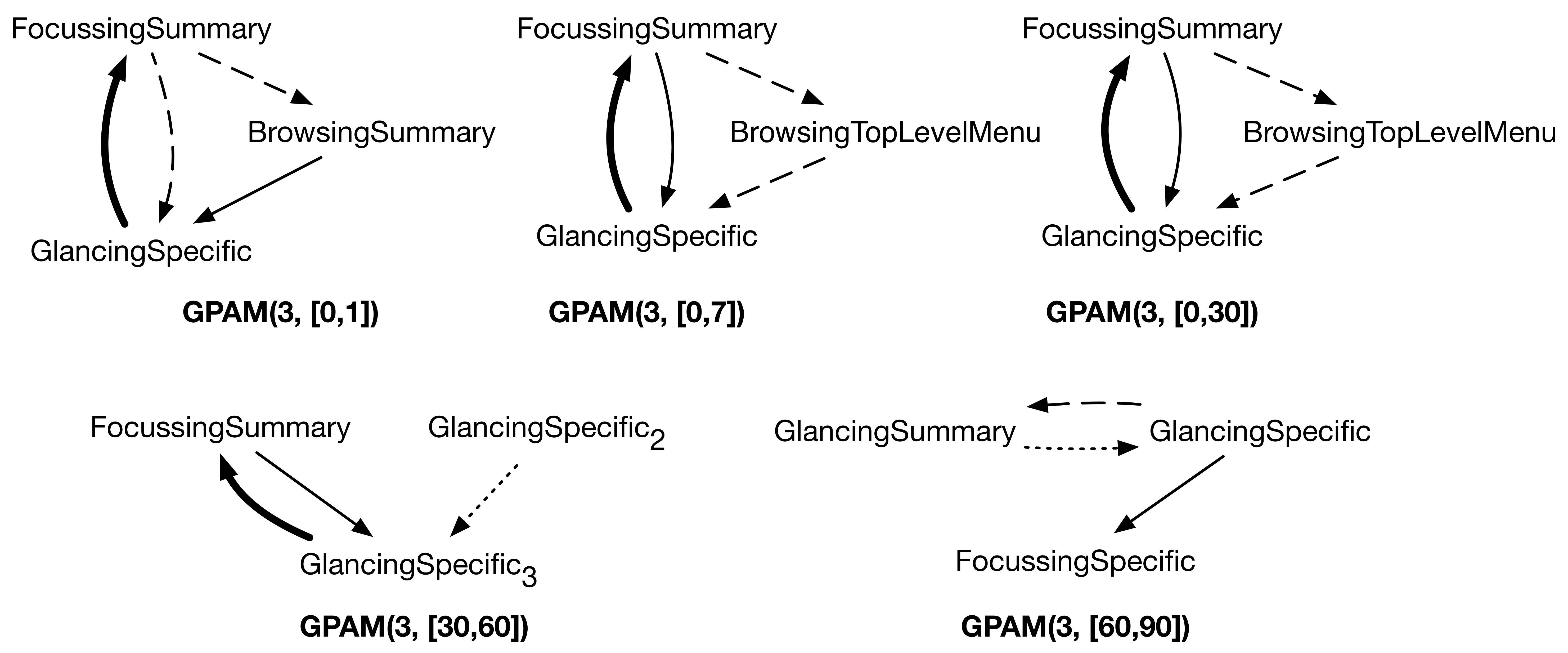
(a) AppTracker1

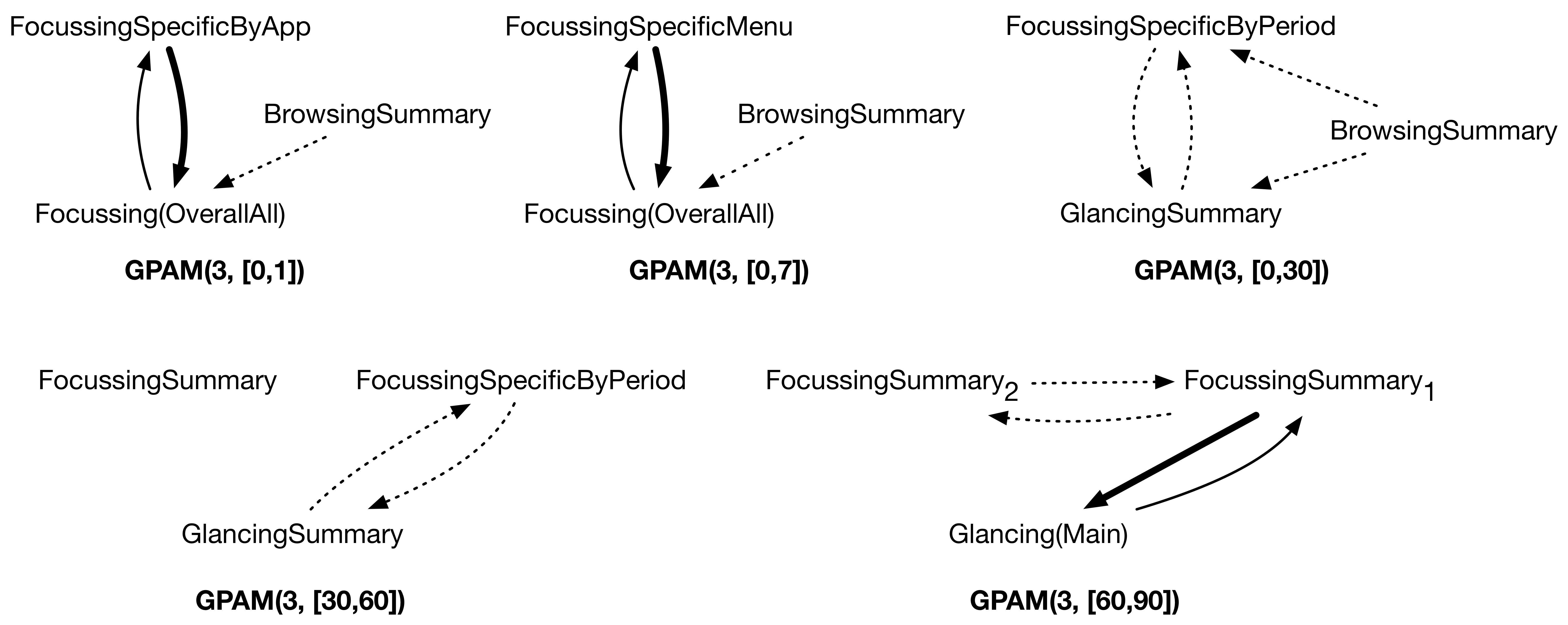
(b) AppTracker2

Figure 9: AppTracker1 and AppTracker2. Visualisations of StateToPattern: the average likelihood of changing activity pattern from an observed state within a session in GPAM(3) models for different time intervals. Excepting the Stats and ChartStats states for which the property returns lower probabilities than the average, the probabilities returned for all states are very similar. Dotted arrows denote probabilities in $[0.02,0.2)$, dashed arrows in $(0.2,0.5)$, thin arrows in $[0.5,0.8)$, and thick arrows $\geq 0.8$. Likelihoods lower than 0.02 are omitted. For GPAM(3,[30,60]) in AppTracker1 we distinguish the two identically-labelled patterns with subscript $2$ or $3$, indicating pattern identifier (AP2 or AP3).

Figure 10 shows the results of the LongRunPattern property for different GPAM(3) models for AppTracker1 and AppTracker2. In the early days usage models, FocussingSummary and GlancingSpecific are equally likely and prevailing, compared with BrowsingSummary and FocussingSpecific. In the second month, the probability of being in GlancingSpecific centred on Last7Days and SelectPeriod is higher than being in GlancingSpecific centred on Last7Days, AppsInPeriod, and SelectPeriod (0.38 compared to 0.18, respectively); however, overall Glancing behaviour in the Last7Days and SelectPeriod sub-menus is more prevalent than Focussing behaviour centred on the (typically exploratory) Summary states OverallUsage and Stats. In the third month, FocussingSpecific prevails, as in GPAM(2). However we see for the first time Glancing between OverallUsage and Stats, which could indicate that while the sessions may be short, they may not be exploratory but indicate more purposeful user intent. We conclude that viewing of Specific states becomes a more Focussing behaviour for experienced usage.

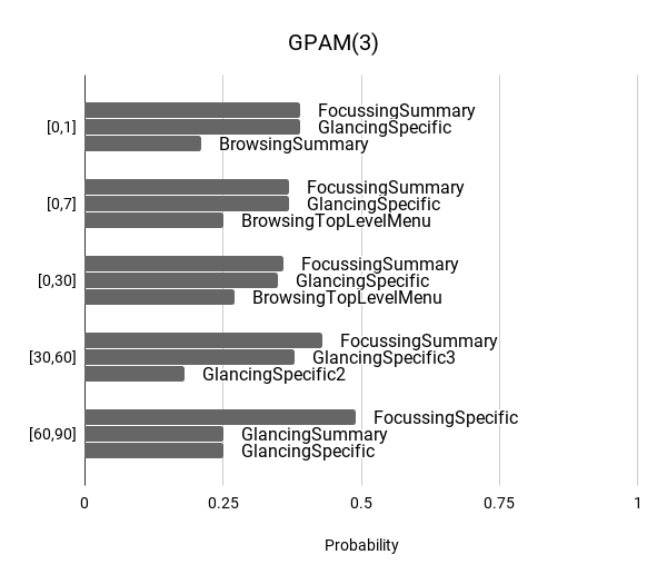
(a) AppTracker1

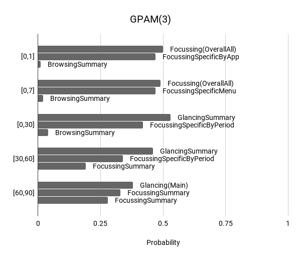
(b) AppTracker2

Figure 10: AppTracker1 and AppTracker2. Visualisation of probabilities of being in each activity pattern in the long run in GPAM(3) models for different time intervals; the entries are ordered decreasingly for each time interval.

References

- [1] O. Andrei and M. Calder. Data-driven modelling and probabilistic analysis of interactive software usage. Journal of Algebraic and Logical Methods in Programming (JLAMP), 100:195–214, 2018.
- [2] O. Andrei, M. Calder, M. Chalmers, A. Morrison, and M. Rost. Probabilistic Formal Analysis of App Usage to Inform Redesign. In E. Ábrahám and M. Huisman, editors, Proc. of iFM’16, volume 9681 of Lecture Notes in Computer Science, pages 115–129. Springer, 2016.
- [3] O. Andrei, M. Calder, M. Higgs, and M. Girolami. Probabilistic Model Checking of DTMC Models of User Activity Patterns. In G. Norman and W. H. Sanders, editors, Proc. of QEST 2014, volume 8657 of Lecture Notes in Computer Science, pages 138–153. Springer, 2014.
- [4] S. Attfield, G. Kazai, M. Lalmas, and B. Piwowarski. Towards a science of user engagement (Position Paper). In Pre-proceeding of the ACM WSDM Workshop on User Modelling for Web Applications , pages 9–12, 2011.
- [5] C. Baier and J.-P. Katoen. Principles of Model Checking. The MIT Press, 2008.
- [6] N. Banovic, C. Brant, J. Mankoff, and A. K. Dey. ProactiveTasks: the short of mobile device use sessions. In A. J. Quigley, S. Diamond, P. Irani, and S. Subramanian, editors, Proceedings of the 16th international conference on Human-computer interaction with mobile devices & services (MobileHC’14), pages 243–252. ACM, 2014.
- [7] N. Banovic, T. Buzali, F. Chevalier, J. Mankoff, and A. K. Dey. Modeling and Understanding Human Routine Behavior. In J. Kaye, A. Druin, C. Lampe, D. Morris, and J. P. Hourcade, editors, Proceedings of the 2016 CHI Conference on Human Factors in Computing Systems, pages 248–260. ACM, 2016.
- [8] F. Benevenuto, T. Rodrigues, M. Cha, and V. A. F. Almeida. Characterizing user behavior in online social networks. In A. Feldmann and L. Mathy, editors, Proceedings of the 9th ACM SIGCOMM Internet Measurement Conference (IMC’09), pages 49–62. ACM, 2009.
- [9] H. Bojinov, Y. Michalevsky, G. Nakibly, and D. Boneh. Mobile device identification via sensor fingerprinting. CoRR, abs/1408.1416, 2014.
- [10] J. Borges and M. Levene. Data Mining of User Navigation Patterns. In B. Masand and M. Spiliopoulou, editors, Web Usage Analysis and User Profiling: International WEBKDD’99 Workshop, pages 92–112. Springer, 2000.
- [11] J. F. Bowring, J. M. Rehg, and M. J. Harrold. Active learning for automatic classification of software behavior. In G. S. Avrunin and G. Rothermel, editors, Proceedings of the International Symposium on Software Testing and Analysis (ISSTA’04), pages 195–205. ACM, 2004.
- [12] N. Busany and S. Maoz. Behavioral log analysis with statistical guarantees. In Proceedings of the 38th International Conference on Software Engineering, (ICSE’16), pages 877–887. ACM, 2016.
- [13] X. Chen, G. Bailly, D. P. Brumby, A. Oulasvirta, and A. Howes. The Emergence of Interactive Behavior: A Model of Rational Menu Search. In B. Begole, J. Kim, K. Inkpen, and W. Woo, editors, Proceedings of the 33rd Annual ACM Conference on Human Factors in Computing Systems (CHI’15), pages 4217–4226. ACM, 2015.
- [14] F. Chierichetti, R. Kumar, P. Raghavan, and T. Sarlós. Are web users really Markovian? In A. Mille, F. L. Gandon, J. Misselis, M. Rabinovich, and S. Staab, editors, Proceedings of the 21st World Wide Web Conference 2012 (WWW’12), pages 609–618. ACM, 2012.
- [15] K. Church, D. Ferreira, N. Banovic, and K. Lyons. Understanding the Challenges of Mobile Phone Usage Data. In S. Boring, E. Rukzio, H. Gellersen, and K. Hinckley, editors, Proceedings of the 17th International Conference on Human-Computer Interaction with Mobile Devices and Services (MobileHCI’15), pages 504–514. ACM, 2015.
- [16] J. E. Cook and A. L. Wolf. Discovering Models of Software Processes from Event-Based Data. ACM Trans. Softw. Eng. Methodol., 7(3):215–249, 1998.
- [17] A. P. Dempster, N. M. Laird, and D. B. Rubin. Maximum Likelihood from Incomplete Data via the EM Algorithm. Journal of the Royal Statistical Society. Series B (Methodological), 39(1):1–38, 1977.
- [18] A. J. Dix. Designing for appropriation. In T. C. Ormerod and C. Sas, editors, Proceedings of the 21st British HCI Group Annual Conference on People and Computers: HCI…but not as we know it - Volume 2, BCS-HCI’07, pages 27–30. British Computer Society, 2007.
- [19] P. Dourish. The Appropriation of Interactive Technologies: Some Lessons from Placeless Documents. Computer Supported Cooperative Work (CSCW), 12(4):465–490, 2003.
- [20] S. S. Emam and J. Miller. Inferring Extended Probabilistic Finite-State Automaton Models from Software Executions. ACM Trans. Softw. Eng. Methodol., 27(1):4:1–4:39, 2018.
- [21] X. Ferre, E. Villalba, H. Julio, and H. Zhu. Extending mobile app analytics for usability test logging. In IFIP Conference on Human-Computer Interaction INTERACT 2017, pages 114–131. Springer, 2017.
- [22] D. Ferreira, J. Gonçalves, V. Kostakos, L. Barkhuus, and A. K. Dey. Contextual experience sampling of mobile application micro-usage. In A. J. Quigley, S. Diamond, P. Irani, and S. Subramanian, editors, Proceedings of the 16th international conference on Human-computer interaction with mobile devices & services, MobileHCI 2014, Toronto, ON, Canada, September 23-26, 2014, pages 91–100. ACM, 2014.
- [23] C. Ghezzi, M. Pezzè, M. Sama, and G. Tamburrelli. Mining Behavior Models from User-Intensive Web Applications. In P. Jalote, L. C. Briand, and A. van der Hoek, editors, Proc. of ICSE’14, pages 277–287. ACM, 2014.
- [24] M. Girolami and A. Kabán. Simplicial Mixtures of Markov Chains: Distributed Modelling of Dynamic User Profiles. In S. Thrun, L. K. Saul, and B. Schölkopf, editors, Advances in Neural Information Processing Systems 16 (NIPS’03), pages 9–16. MIT Press, 2004.
- [25] M. Hall, M. Bell, A. Morrison, S. Reeves, S. Sherwood, and M. Chalmers. Adapting ubicomp software and its evaluation. In T. C. N. Graham, G. Calvary, and P. D. Gray, editors, Proc. of EICS’09, pages 143–148. ACM, 2009.
- [26] A. Howes, X. Chen, A. Acharya, and R. L. Lewis. Interaction as an Emergent Property of a Partially Observable Markov Decision Process. In A. Oulasvirta, P. O. Kristensson, X. Bi, and A. Howes, editors, Computational Interaction, chapter 10, pages 287–310. Oxford Scholarship, 2018.
- [27] S. S. Intille, J. Rondoni, C. Kukla, I. Ancona, and L. Bao. A context-aware experience sampling tool. In G. Cockton and P. Korhonen, editors, Extended abstracts of the 2003 Conference on Human Factors in Computing Systems (CHI’03), pages 972–973. ACM, 2003.
- [28] G. F. Jenks. The Data Model Concept in Statistical Mapping. International Yearbook of Cartography 7, pages 186–190, 1967.
- [29] S. L. Jones, D. Ferreira, S. Hosio, J. Gonçalves, and V. Kostakos. Revisitation analysis of smartphone app use. In K. Mase, M. Langheinrich, D. Gatica-Perez, H. Gellersen, T. Choudhury, and K. Yatani, editors, Proceedings of the 2015 ACM International Joint Conference on Pervasive and Ubiquitous Computing (UbiComp’15). ACM, 2015.
- [30] V. Kostakos, D. Ferreira, J. Gonçalves, and S. Hosio. Modelling smartphone usage: a Markov state transition model. In P. Lukowicz, A. Krüger, A. Bulling, Y. Lim, and S. N. Patel, editors, Proceedings of the 2016 ACM International Joint Conference on Pervasive and Ubiquitous Computing (UbiComp’16), pages 486–497, 2016.
- [31] M. Z. Kwiatkowska, G. Norman, and D. Parker. PRISM 4.0: Verification of Probabilistic Real-Time Systems. In G. Gopalakrishnan and S. Qadeer, editors, Proc. of CAV’11, volume 6806 of LNCS, pages 585–591. Springer, 2011.
- [32] I. Li, A. Dey, and J. Forlizzi. A Stage-based Model of Personal Informatics Systems. In E. D. Mynatt, D. Schoner, G. Fitzpatrick, S. E. Hudson, W. K. Edwards, and T. Rodden, editors, Proceedings of the 28th International Conference on Human Factors in Computing Systems (CHI’10), pages 557–566. ACM, 2010.
- [33] L. Lu, M. H. Dunham, and Y. Meng. Mining Significant Usage Patterns from Clickstream Data. In O. Nasraoui, O. R. Zaïane, M. Spiliopoulou, B. Mobasher, B. M. Masand, and P. S. Yu, editors, Proceedings of the 7th International Workshop on Knowledge Discovery on the Web (WebKDD 2005), pages 1–17. Springer, 2005.
- [34] K. S. Luckow and C. S. Pasareanu. Log2model: inferring behavioral models from log data. In Proceedings of the 18th IEEE International High-Level Design Validation and Test Workshop (HLDVT’16), pages 25–29. IEEE, 2016.
- [35] D. McMillan, A. Morrison, O. Brown, M. Hall, and M. Chalmers. Further into the Wild: Running Worldwide Trials of Mobile Systems. In P. Floréen, A. Krüger, and M. Spasojevic, editors, Proceedings of the 8th international conference on Pervasive Computing (Pervasive 2010), volume 6030 of Lecture Notes in Computer Science, pages 210–227. Springer, 2010.
- [36] A. L. Montgomery, S. Li, K. Srinivasan, and J. C. Liechty. Modeling online browsing and path analysis using clickstream data. Marketing science, 23(4):579–595, 2004.
- [37] A. Morrison, X. Xiong, M. Higgs, M. Bell, and M. Chalmers. A large-scale study of iphone app launch behaviour. In Proceedings of the 2018 CHI Conference on Human Factors in Computing Systems, CHI ’18, pages 344:1–344:13, New York, NY, USA, 2018. ACM.
- [38] K. P. Murphy. Machine Learning: A Probabilistic Perspective. The MIT Press, 2012.
- [39] A. Oulasvirta, T. Rattenbury, L. Ma, and E. Raita. Habits make smartphone use more pervasive. Personal and Ubiquitous Computing, 16(1):105–114, 2012.
- [40] J. Rooksby, P. Asadzadeh, A. Morrison, C. McCallum, C. Gray, and M. Chalmers. Implementing ethics for a mobile app deployment. In H. B. L. Duh, C. Lueg, M. Billinghurst, and W. Huang, editors, Proceedings of the 28th Australian Conference on Computer-Human Interaction (OzCHI’16), OzCHI ’16, pages 406–415. ACM, 2016.
- [41] P. Singer, D. Helic, A. Hotho, and M. Strohmaier. HypTrails: A Bayesian Approach for Comparing Hypotheses About Human Trails on the Web. In A. Gangemi, S. Leonardi, and A. Panconesi, editors, Proceedings of the 24th International Conference on World Wide Web, WWW 2015, pages 1003–1013. ACM, 2015.
- [42] P. Singer, D. Helic, B. Taraghi, and M. Strohmaier. Detecting Memory and Structure in Human Navigation Patterns Using Markov Chain Models of Varying Order. PLOS ONE, 9(7):1–21, 2014.
- [43] J. Stragier, G. Vandewiele, P. Coppens, F. Ongenae, W. Van den Broeck, F. De Turck, and L. De Marez. Data Mining in the Development of Mobile Health Apps: Assessing In-App Navigation Through Markov Chain Analysis. J. Med. Internet Res., 21(6), Jun 2019.
- [44] P. Tchounikine. Designing for appropriation: A theoretical account. Human–Computer Interaction, 32(4):155–195, 2017.
- [45] H. W. Thimbleby, P. A. Cairns, and M. Jones. Usability analysis with Markov models. ACM Trans. Comput.-Hum. Interact., 8(2):99–132, 2001.
- [46] D. R. Thomas. A General Inductive Approach for Analyzing Qualitative Evaluation Data. American Journal of Evaluation, 27(2):237–246, 2006.
- [47] V. Tran, D. Maxwell, N. Fuhr, and L. Azzopardi. Personalised Search Time Prediction using Markov Chains. In J. Kamps, E. Kanoulas, M. de Rijke, H. Fang, and E. Yilmaz, editors, Proceedings of the ACM SIGIR International Conference on Theory of Information Retrieval (ICTIR’17), pages 237–240. ACM, 2017.
- [48] J. Wang, J. Sun, Q. Yuan, and J. Pang. Should We Learn Probabilistic Models for Model Checking? A New Approach and An Empirical Study. In M. Huisman and J. Rubin, editors, Proceedings of the 20th International Conference on Fundamental Approaches to Software Engineering (FASE’17), volume 10202 of Lecture Notes in Computer Science, pages 3–21. Springer, 2017.
- [49] L. Welch. Hidden Markov Models and the Baum-Welch Algorithm. IEEE Information Theory Society Newsletter, December 2003.
- [50] J. A. Whittaker and J. H. Poore. Markov Analysis of Software Specifications. ACM Trans. Softw. Eng. Methodol., 2(1):93–106, 1993.
- [51] G. Wolf. Know Thyself: Tracking Every Facet of Life, from Sleep to Mood to Pain, 24/7/365. https://www.wired.com/2009/06/lbnp-knowthyself/, 2009. Accessed: 2021-06-01.
- [52] S. Zhao, J. Ramos, J. Tao, Z. Jiang, S. Li, Z. Wu, G. Pan, and A. K. Dey. Discovering Different Kinds of Smartphone Users through Their Application Usage Behaviors. In Proceedings of the 2016 ACM International Joint Conference on Pervasive and Ubiquitous Computing (UbiComp’16), pages 498–509. ACM, 2016.