Augmented Electronic Ising Machine as an Effective SAT Solver

Abstract

With the slowdown of improvement in conventional von Neumann systems, increasing attention is paid to novel paradigms such as Ising machines. They have very different approach to NP-complete optimization problems. Ising machines have shown great potential in solving binary optimization problems like MaxCut. In this paper, we present an analysis of these systems in satisfiability (SAT) problems. We demonstrate that, in the case of 3-SAT, a basic architecture fails to produce meaningful acceleration, thanks in no small part to the relentless progress made in conventional SAT solvers. Nevertheless, careful analysis attributes part of the failure to the lack of two important components: cubic interactions and efficient randomization heuristics. To overcome these limitations, we add proper architectural support for cubic interaction on a state-of-the-art Ising machine. More importantly, we propose a novel semantic-aware annealing schedule that makes the search-space navigation much more efficient than existing annealing heuristics. With experimental analyses, we show that such an Augmented Ising Machine for SAT (AIMS), outperforms state-of-the-art software-based, GPU-based and conventional hardware SAT solvers by orders of magnitude. We also demonstrate AIMS to be relatively robust against device variation and noise.

I Introduction

As complexity of semiconductor fabrication technology reaches unprecedented levels, there is an increasing urgency to seek other sources of improvement to speed and cost of computing systems. Physics-based computing systems are getting increasing attention from the architecture community. Quantum computing has some interesting features such as changing how problem complexity scales with size [70, 35]. Nevertheless, the technical challenges of building large-scale error-corrected systems remain formidable.

Another area that has seen rapid recent progress is the subfield loosely termed Ising machines. These machines are dynamical systems that can achieve extremely fast and energy-efficient search of an “energy landscape” defined by a parameterized Ising model. This has the effect of optimizing the Ising model or the equivalent of a QUBO (quadratic unconstrained binary optimization) form. While the search can involve quantum mechanics (as done in quantum annealers from D-Wave), it can also be done classically.

While functioning prototypes are only beginning to emerge, many Ising machine design concepts exist. For those that operate in the classical regime, scaling in size appears less challenging than gate-based quantum computers. For example, NTT recently developed a 100,000-node Coherent Ising Machine (CIM) [40]. Consequently, it is conceivable that these machines can already outperform state-of-the-art sequential solvers. However, as we will discuss in more detail, there are more subtle issues beyond just scaling mentioned above.

We first take an application-centric perspective to the analysis of these machines: to what extent can they accelerate solving real-world problems. One such well known problem that appears in many applications is boolean satisfiability (SAT), which attempts to find a satisfying assignment for a given logical statement [16]. While Sec. II discusses SAT in more detail, we note here that it is an excellent benchmark: While many applications can be mapped into a QUBO problem, there are nuances (e.g., efficient navigation and cubic interactions); in the case of SAT problems, the nuances have important implication on a machine’s capabilities as we will discuss later.

The main contributions of this paper can be summarized as follows. ① We demonstrate that standard Ising machines are not competitive in solving SAT compared to state-of-the-art SAT solvers. Our analysis show that the main causes are lack of support for high order interaction and efficient search-space navigation. ② Motivated by these limitations, we extend a baseline Ising machine to support high order terms. ③ But more importantly, we propose a new semantic-aware annealing heuristic to significantly improve Ising machines’ navigational efficiency. ④ We demonstrate that our proposed “augmented” Ising machine is indeed orders of magnitude faster than existing state-of-the-art SAT solvers.

For the convenience of the reader, a table of frequent acronyms follows:

BRIM	Bistable Resistively-coupled Ising Machine
CDCL	Conflict-Driven Clause Learning
KZFD	Kolmogorov, Zabih, Freedman, Drineas
QUBO	Quadratic Unconstrained Binary Optimization

CNF	Conjunctive Normal Form
QC	Quantum Computing
SA	Simulated Annealing
TTS	Time-To-Solution

II Background and Related Work

II-A Boolean Satisfiability (SAT)

Boolean satisfiability has a large domain of application including circuit hardware verification [15], cryptographic protocols [9], software verification [43], hierarchical planning [65], mapping [51], scheduling [26], and even hardware security attacks [68, 84].

A generic SAT problem asks whether a propositional logic formula F is satisfiable for some mapping of variables to truth values [16]. F consists of boolean-valued variables acted on by unary logical operator (negation: $\lnot$) or binary ones (and: $\land$; or: $\lor$; and implications: $\to$, $\iff$) (e.g., $F=x_{1}\lor(\lnot x_{2})\land(x_{3}\to x_{4})$) The statement is typically expressed in Conjunctive Normal Form (CNF) [16], i.e., a logical conjunction of separate clauses (e.g., $F=C_{1}\land C_{2}\land C_{3}$). Each clause is a logical disjunction of a number of literals. Literals are boolean variables or their negations (e.g., $C=x_{1}\lor\overline{x_{2}}\lor x_{3}$). Propositional logic statements can be converted to CNF in linear time by introducing new variables and clauses  [78]. When the number of literals in any clause is no more than $k$, the problem is called $k$-SAT. When $k\geq 3$, the problem is NP-complete. 3-SAT can be used to formulate any NP-complete problem in standard CNF format, with SAT solvers as an efficient means of solution [57, 27].

II-B Software SAT solvers

In the worst case, the deterministic evaluation of a SAT problem requires enumeration of all possible variable truth values. Correspondingly, a naive deterministic SAT algorithm is $O(2^{N})$ for an $N$-variable formula. Hence, modern SAT solvers rely on partial search-space exploration to attempt to find satisfying solutions. While a more comprehensive review can be found in [16], the more relevant point to this paper is that there are two primary paradigms for SAT algorithms.

Most contemporary SAT solvers are based upon the Conflict-Driven Clause Learning (CDCL) algorithm [53] (an extension of DPLL algorithm [30]). CDCL is a sequential approach in which variables are incrementally assigned values until either all variables are assigned (SAT) or a conflict is reached (all literals of a clause are false). Conflicts cause search-space backtracking. Modern incarnations rely heavily on heuristics to trim the search space and prioritize promising decision branches. KISSAT [17] is a prime example. Its variants have won the SAT solver competition from 2020 to 2022  [1, 18].

The second class are known broadly as “stochastic local search” (SLS) algorithms, which perform localized random walks over the search space. A paradigmatic example is WalkSAT [47], an extended version of Schöning’s algorithm [64]. Rather than explicitly trimming the search space, SLS algorithms attempt to maximize the probability of encountering a satisfying solution with stochastic mechanisms. WalkSAT has an expected time complexity of $O(1.334^{N})$ – a polynomial improvement over $O(2^{N})$ [64], which has later been improved to $O(1.308^{N})$ with the PPSZ algorithm  [63]. SLS algorithms run until either a SAT is found or a timeout. Therefore, they cannot refute a CNF formula and are classified as incomplete solvers, without a guarantee of success. Note that in practice, even complete solvers are generally used with a timeout to prevent excessive runtime from full exponential search space exploration.

Hybrid solvers mixing CDCL and SLS have been shown to be highly effective [1, 13]. The close analogy between Ising machines and SAT heuristics was also exploited in a hybrid CDCL/Ising machine-based approach [75].

II-C Conventional hardware SAT solvers

Hardware SAT solvers can also be classified by its general algorithm into CDCL or SLS styles. The former is further separated into coprocessors (e.g., handling only boolean constraint propagation [29]) and dedicated solvers (e.g., [36]). While a 2017 survey [71] contains a good summary of earlier works, a few recent works have focused on SLS style algorithms such as probSAT [10] and AmoebaSAT [8]. These algorithms are easier to implement in hardware and expose more parallelism leading to orders of magnitudes of speedups over the respective software version [69, 56, 38]. Note that as discussed earlier, software speeds vary dramatically. As a result, speedups over a particular software solver is not a conclusive evidence. Finally, like their software counterpart, SLS-style hardware lack the completeness guarantees.

II-D Optimization using quantum computing

Quantum computing (QC) methods have been previously proposed for NP-Complete problems. There are two broad, theoretically equivalent categories of QC [4]: ① gate-based QC or “Universal Quantum Computing (UQC)” and ② “Adiabatic Quantum Computing (AQC)”. UQC algorithms perform sequences of unitary operations on quantum bits (qubits) before sampling their state. Grover’s algorithm for unstructured search [35] is a popular example. However, error sensitivity in the “Noisy-Itermediate Scale Quantum” (NISQ) era limit its immediate usefulness [81]. Noise-resilient, “shallow” algorithms have been proposed for SAT as well [14]. Examples are generally hybrid algorithms, either classically optimizing a parametric quantum circuit [32, 20] or using limited QC subroutines [31]. However, these proposals have either used noiseless simulations [20] or were purely theoretical [31], so their real-world applicability is unknown.

AQC algorithms evolve qubits under a mixture of two non-commuting Hamiltonians: a “simple” operator with a known ground state and a problem-specific cost function. Ideally, one begins in the ground state of the simple Hamiltonian and slowly transitions to the other. The adiabatic theorem provides ground state guarantees for sufficiently slow transitions [5]. Adiabatic algorithms for SAT have been proposed which theoretically promise high-quality solutions [25, 24]. However, NISQ-era noise precludes adiabaticity [14]. A relaxation is “quantum annealing” (QA): retaining mixed operators but abandoning theoretical guarantees [45]. In QA, the transverse field decreases over the course of system evolution similar to classical simulated annealing [48]. QA was shown to satisfy 24/100 3-SAT instances. Testing was limited to 10-variable problems due to QA topology constraints [34, 73] as we will discuss in Sec. III-B.

Throughout the analyses, we will report the performance of an optimistic estimate of a near-term quantum algorithm. As we will see, such approaches do not seem to offer any benefit in the NISQ era.

II-E Ising machines

The Ising model was originally used to describe the Hamiltonian ($H$) for a state of spins on some lattice. A modified version (Eq. 1) of the formula is more useful in the discussion of optimization problems.

$$\begin{split}H(\sigma)&=-\sum_{(i,j)}J_{ij}\sigma_{i}\sigma_{j}-\sum_{i}h_{i}\sigma_{i}=-\sigma^{\top}J\sigma-h^{\top}\sigma\end{split}$$ (1)

A loose physical analogy is as follows. A system of spins ($\sigma_{i}\in\{-1,+1\}$) are subject to the influence of a set of parameters $J_{ij}$ and $h_{i}$. $J_{ij}$ describes the coupling between two spins ($\sigma_{i}$ and $\sigma_{j}$), while $h_{i}$ describes the influence of an external magnetic field on spin $\sigma_{i}$. Given this setup, the spins will naturally gravitate towards the lowest energy state (ground state). Technically, the probability of each state follows the Boltzmann distribution:

$$P(\sigma)\propto e^{-\frac{H(\sigma)}{T}}$$ (2)

If a physical system of spins can be set up subject to the programmable parameters, then we gradually lower the temperature ($T$) of the system (annealing); when it approaches 0, the probability of the system in ground state(s) will approach 1. Such a physical system is thus effectively performing an optimization (where the objective function is Eq. 1). In practice, different types of physics are involved to achieve the effective optimization. These physical systems are often referred to as Ising machines and have been shown to find good solutions to combinatorial optimization problems (COP) at extraordinary speeds [40, 41, 83, 54, 74, 19, 79, 3].

In principle, all NP-complete problems can be converted into a COP and thus benefit from the speed and efficiency of an Ising machine. Indeed, [52] is often cited for this purpose. In practice, however, there are subtle issues in the process of solving a problem with an Ising machine:

1. A “native” formulation of the problem may contain cubic or higher-order terms. Converting them down to quadratic form increases the number of spins needed.

2. In many prototypes, coupling is only limited to between nearby spins. This means even more auxiliary spins are needed.

3. The navigation through the energy landscape is purely based on the formulation. Any problem-specific insight may be lost.

In response to the first issue, a number of proposals for “high order” Ising models have recently been proposed. High order models expand the Ising Hamiltonian to arbitrary polynomial degree. Efforts so far have focused on 3^rd and 4^th order interactions, with applications both to 3-SAT and its variants  [11, 21], and hypergraph partitioning [12]. Ising models generalized to $K$-degree interactions are of the form [23]:

$$\begin{split}H(\sigma)=&-\sum_{i}h_{i}\sigma_{i}-\sum_{(i,j)}J^{(2)}_{ij}\sigma_{i}\sigma_{j}-\sum_{(i,j,k)}J^{(3)}_{ijk}\sigma_{i}\sigma_{j}\sigma_{k}\\ &\dots-\sum_{(i,j,...,m)}J^{(K)}_{ij...m}\sigma_{i}\sigma_{j}...\sigma_{m}\end{split}$$ (3)

High order Ising Hamiltonians can be applied to a broader class of problems, collectively denoted as “polynomial unconstrained binary optimization” (PUBO) [23, 76] or “higher-order unconstrained binary optimization” (HUBO) [44, 59].

Simulation of high order Ising machines have been shown to outperform the respective baseline Ising machine solvers. The GPU/FPGA based simulated bifurcation algorithm, originally limited to quadratic systems, has been modified to allow for more general Hamiltonians [46]. An optical Ising machine-inspired algorithm demonstrated solution quality superior to existing algorithms, though without significant speedup [23].

Amongst nature-based Ising machines, oscillator-based dynamical models have been among the first demonstrated. 3^rd order models were proposed and modeled for classic 3-SAT and “Not-All-Equal” (NAE) 3-SAT problems, with successful demonstration on (tiny) 6-variable problems [11]. An LC oscillator-based model was shown in simulations to solve 3-SAT problems of up to 250 variables, though with poor success rate of 2%[21].

So far, high order Ising machines proposed only added high order couplings. As we will discuss in Sec. III, adding support for cubic interaction alone is insufficient for Ising machines to become competitive as a SAT solver. As discussed in Sec. II-B, there exists a huge amount of background work on SLS for SAT (PPSZ being the fastest known). These solve SAT much more efficiently (visiting less phase points, as we shall see) than an Ising machine that relies on a problem-agnostic annealing schedule. In the next section, we will discuss the challenges in more detail which will motivate us to propose a fast, high order Ising machine that uses a novel annealing schedule.

III Binary Optimization Approach to SAT

In an $N$-variable unconstrained binary optimization (UBO) problem, there are $2^{N}$ possible states $(x_{1},x_{2},...,x_{N}),x_{n}\in\{0,1\}$. Each state is associated with a value of an objective function. The value can be thought of as a cost or energy to be minimized. If the cost function is quadratic or higher-order polynomial, the problem is called QUBO or PUBO, respectively. Given that each state (or phase point) has an energy level, the entire phase space can be thought of as an energy landscape. Consider a 3-SAT problem in CNF: $F=\bigwedge_{i=1}^{{}_{M}}(\ell_{i1}\lor\ell_{i2}\lor\ell_{i3})$, where each term $\ell_{ij}$ is a literal $x_{n}$ or $\bar{x}_{n}$. We can simply define the energy for each phase point as the number of unsatisfied clauses of that phase point. If we use 1 and 0 to represent true or false of each Boolean variable $x_{n}$, then the energy (or the objective function to be minimized) is

$$\begin{split}H=\sum_{i=1}^{M}(1-\ell_{i1})(1-\ell_{i2})(1-\ell_{i3});\\ \underline{e.g.,\ (x_{7}\lor\bar{x}_{11}\lor x_{12})\xrightarrow{}(1-x_{7})x_{11}(1-x_{12})}.\end{split}$$ (4)

Given this energy landscape, a generic algorithm (e.g., simulated annealing or SA) can thus be used as an optimizer. An Ising machine can be thought of as a potentially very efficient alternative to von Neumann hardware running SA. However, there are 3 issues mentioned in Sec. II-E. We now discuss them with more quantitative detail.

III-A Cost of QUBO formulation

While we use binary objective functions because of their straightforward connection with Boolean logic, we note that the standard Ising formulation (Eq. 1) is completely convertible to and from QUBO formulations, by simple conversion between spin and bit representations ($\sigma_{i}=2x_{i}-1;\sigma_{i}\in\{-1,1\}$, $x_{i}\in\{0,1\}$). However, as can be seen in Eq. 4, the objective function has cubic terms $\ell_{i1}\ell_{i2}\ell_{i3}$ and is thus not a QUBO formula. A standard practice is to reduce such an objective function to quadratic form (QUBO) at the expense of extra auxiliary variables. Perhaps the most widely used approach (due to Rosenberg  [62]) is to add a new variable $z$ as a substitute for $x_{1}x_{2}$ and introduce a penalty when $z\neq x_{1}x_{2}$. With this substitution, the cubic term is replaced by a purely quadratic expression:

$$\begin{split}\pm x_{1}x_{2}x_{3}&\rightarrow\pm zx_{3}+k(x_{1}x_{2}-2(x_{1}+x_{2})z+3z),\end{split}$$ (5)

where $k>1$. This seemingly small change has a significant impact. Every clause will generate an extra spin, leading to a total of $M+N$ spins for an $N$-variable, $M$-clause problem. Unfortunately, for the most difficult SAT problems, $M$ is usually around $\alpha_{c}=4.17$ times that of $N$ [58]. This means the number of spins will roughly quintuple and the size of the phase space will grow from $2^{N}$ to $2^{5N}$. After carefully analyzing how the landscape reacts to the penalty, we realized that the Rosenberg substitution can be improved. As it turns out, our improved version is merely reinventing the wheel of KZFD [49, 33]. This formulation has two different substitutions depending on the sign of the cubic term (Eq. 6).

$$\begin{split}-x_{1}x_{2}x_{3}&\rightarrow(2-x_{1}-x_{2}-x_{3})z\\ +x_{1}x_{2}x_{3}&\rightarrow(1+x_{1}-x_{2}-x_{3})z+x_{2}x_{3}\end{split}$$ (6)

To show the impact of quadratization, we will show how the solution time grows (dramatically) as the problem size increases. To more accurately reflect solution time (since the algorithm is stochastic), we use Time-To-Solution (TTS) [37], defined as the expected time to find a solution with 99% probability. Over multiple instances with runtime of $T_{run}$ and a success probability of $P$, TTS can be calculated using Eq. 7.

$$TTS=\begin{cases}T_{run}\times\dfrac{\log_{10}(0.01)}{\log_{10}(1-P)}&P<0.99\\ T_{run}&\textrm{otherwise}\end{cases}$$ (7)

We plot TTS of SA using both cubic formula (SAc) directly (Eq. 4) and the QUBO translation (SAq) with the KZFD and Rosenberg rules in Fig. 1 left.

Figure 1: [Left] Time-to-solution for simulated annealing using cubic and quadratic (with Rosenberg and KZFD rules) objective functions. For reference KISSAT is also included. [Right] The average size of QUBO graphs using KZFD and Rosenberg’s formulations for different problem sizes.

Clearly, adding spins is not just costly in hardware, it has a significant impact on the annealer’s ability to navigate the landscape to reach a certain solution quality. The outperformance of SAc over SAq shows we can avoid costs due to quadratization if the hardware can provide cubic interaction.

Fig. 1 right shows the size bloat in both methods of conversion. We can see that to a first approximation, both SAq’s are slower due to significantly larger phase space. Secondarily, when cubic interaction is absent, the KZFD formulation scales slightly better despite having a slightly larger size penalty. This is due to a specific advantage of the resulting energy landscape the detail of which need not concern us in this paper.

Observation 1: Cubic interaction is very useful.

III-B Topological limitations

On top of translation into a QUBO formula, an Ising machine may impose another constraint to the problem formulation and in turn requires additional auxiliary spins. This is the topology of the coupling array. A generic matrix $J$ (Eq. 1) may require any two spins to be coupled. But practical systems have commonly offered only near-neighbor coupling[61, 80]. One reason is that having fewer couplers may allow a (nominally) bigger system under the same hardware budget. But is the trade-off worthwhile? Let us look at a concrete example of Chimera $k_{4,4}$ used in D-Wave 2000Q.

If the problem has a dense coupling matrix, there is no advantage, only disadvantage. And the disadvantage is both clear and substantial. For an $N$-node all-to-all problem, $O(N^{2})$ couplers are needed. With a Chimera topology, we cannot avoid the $O(N^{2})$ couplers (in fact we need more). In addition, having $O(N^{2})$ couplers automatically means $O(N^{2})$ nodes. With more than 2000 nominal spins, the 2000Q can only map a dense problem of size $\leq 64$, assuming all qubits are stable and available. Compared to an all-to-all topology, the Chimera topology ends up using twice as many couplers and 23 times more nodes. Not only is the topology more costly, it fundamentally complicates landscape navigation.

For the 3-SAT problem, the situation is a bit better. The largest problem 2000Q can map (using KZFD formula) is about 42 variables and 178 clauses. At this size, the coupling matrix has a 4% density. Compared to an all-to-all topology (which would have costed about 210 nodes and 22K couplers), Chimera allows about 3x (2K nodes, 6K couplers) hardware savings. However, the price paid for the savings is again clear and significant.

1. A minor embedding process is needed to convert the original problem into one that is compatible to the machine’s topology. This process takes non-trivial extra time. Embedding a 40-variable, 170-clause problem using the D-Wave minorminer heuristic takes over 17 seconds on average: several orders of magnitude more than the annealing time.

2. With about 10x more spins, the transformed problem has a significantly larger phase space. A natural consequence is lower solution quality (recall the discussion in Sec. III-A). To show that the phase space bloat is a major contributing factor, we use an SA solver and compare 3 different objective functions: cubic (Eq. 4), QUBO conversion using KZFD, and that with additional minor embedding for Chimera graph. As Fig. 2 suggests, with every kind of phase space bloat, SA’s performance is significantly degraded.

Figure 2: [Left] Performance of D-Wave, SA running original cubic formula (SAc), quadratic translations SAq (KZFD), and after embedding to $k_{4,4}$. KISSAT is added for reference. [Right] Size of the minimum square $k_{4,4}$ Chimera lattice needed for embedding with the minorminer tool [28] compared with the original KZFD graphs. The minimum Chimera sizes for 100 and 600 variables were extrapolated from the observed quadratic scaling.

Based on our analysis, the take-away point is: for the costs in solution quality and extra processing time, it is not clear a near-neighbor topology such as chimera is providing much benefit even for the extremely sparse problem such as 3-SAT.

Observation 2: Near-neighbor coupling is costly.

III-C Navigational efficiency

It is clear that if the Ising machine hardware can provide support to avoid adding many extra spins and the concomitant phase space bloat, the performance will improve. But can it outperform a conventional software algorithm? That depends on the problem and the algorithm. On the one hand, for a generic problem simply defined as an energy landscape by, say, Eq. 1), the answer is clearly yes. This is because our best algorithm is some variant of SA (e.g., [42]). SA navigates the energy landscape purely by the formula without any additional insight. Our empirical observations suggest that to reach similar solution qualities, both hardware Ising machines and SA need to visit similar number of phase points; and the former can be orders of magnitude faster and more efficient than the latter to visit the same number of phase points.

On the other hand, for problems such as SAT where the landscape is derived, insights from the original problem formulation may not be obvious in the cost function. Software algorithms may explore these insights and arrive at powerful, problem-specific heuristics to more efficiently navigate the phase space. Thus, what software lacks in speed when visiting/evaluating each phase point can be compensated by its “navigational efficiency”, or arriving at the solution by effectively visiting far fewer phases points. We have already seen this in Fig. 2: while SAc was faster than KISSAT for smaller problems, its advantage disappeared as the problem size grew. This slowdown is to some extent explained by navigational efficiency. The assignment propagation in CDCL has the effect of ruling out entire subspaces without explicitly visiting each phase point. Depending on the problem type and size, this can help CDCL style algorithms over SLS.

Observation 3: Navigational efficiency is important.

III-D Summary

To recap: special-purpose hardware such as Ising machines have strengths over conventional software running on von Neumann hardware. But they also face unique engineering challenges and lack the cumulative innovation invested in the state-of-the-art algorithms. Take the SAT problem as a case study, we can see the effect in Fig. 3.

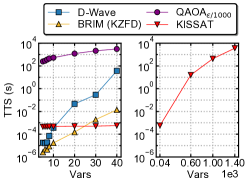
Figure 3: [Left] Execution times of different machines compared with a state-of-the-art SAT solver (KISSAT) for problems with different number of variables (Vars). [Right] Running KISSAT with problem sizes whose TTS matches that of QAOA and D-Wave at 40 variables.

In this figure, we model the speed of BRIM [3], D-Wave 2000Q, and KISSAT, each representing the state of the art in electronic Ising machine, QA, and software solvers. We also plot the optimistic simulation results of Quantum Approximate Optimization Algorithm (QAOA_ϵ/1000) with 1000x lower noise levels ($\epsilon$) than today’s quantum computers. We observe that quantum computing has massive overhead which makes it unlikely to be useful for SAT in the NISQ era. Now looking at BRIM’s results, we see that just like D-Wave 2000Q, BRIM’s early speed advantage quickly disappears as the problem size increases. In their present form, BRIM and D-Wave annealers are unable to be helpful for SAT. Moreover, based on TTS for current software, the minimum for special purpose hardware to become useful is probably around 600 variables. For QA with near-neighbor topology, this translates to around 460,000 qubits. For QAOA, the threshold is “almost noiseless”. In either case, these are goals beyond the NISQ era.

IV Architectural Support

Motivated by the observations so far, we propose a number of architectural supports that allow an electronic Ising machine to regain problem solving efficacy for SAT.

IV-A BRIM as a baseline

The Bistable Resistively-coupled Ising Machine (BRIM) [3] has three properties that make it an ideal starting point for our architectural exploration:

1. CMOS-compatible: This allows for an easy integration with additional architectural support or ultimately with other types of processing elements in an SoC. Moreover, the voltage-based spin representation is easy to work with for additional digital logic, in contrast to more complicated spin representations such as qubits [39], or oscillator phases [41].

2. Efficient dynamical system: Unlike digital annealers that essentially hard-wire a von-Neumann algorithm [82, 77], BRIM is a dynamical system with programmable resistive coupling for nano-scale capacitive spins. It is thus much more efficient due to fundamental reasons. In the original paper [3], the authors have demonstrated significant speedup for BRIM compared to a myriad of existing Ising machines.

3. All-to-all topology: Motivated by observation 2, we opt for an all-to-all topology (for quadratic interactions). With BRIM, this is both easy to achieve (all nodes are simply interconnected via a matrix of coupling units) and quite inexpensive in terms of hardware resources (each coupling unit accounts for only 1 $\mu m^{2}$ chip area with a 45nm Cadence PDK). Moreover, in a recent paper [67], the authors have demonstrated a multiprocessor BRIM that can solve a problem with over 16,000 nodes (all-to-all connected) orders of magnitude faster than any existing solution.

IV-B A bit-based implementation of BRIM

We modify the baseline BRIM design [3] to represent $\{0,1\}$-bits instead of $\{+1,-1\}$ spins. This is because for SAT, the bit representation is more direct and obviates the need for QUBO-to-Ising conversion.

The blue module in Fig. 5 shows the new baseline BRIM design with bit representation. Here, each node represents a variable $x_{n}$ in the 3-SAT formula, and each coupling unit $q_{nj}$ and $l_{n}$ represents the quadratic and linear interactions respectively. The coupling resistance is given by $R_{nj}=\frac{R}{|q_{nj}|}$, where $R$ is a constant and $q_{nj}$ is the coupling between nodes $n$ and $j$. The sign of the coupling is interpreted as follows: ① if $q_{nj}>0$, then the nodes are connected in parallel (output of a node is connected to the positive input terminal of the other node via resistance $R_{nj}$ : $Out_{n}\rightarrow IN^{+}_{j}$, $Out_{j}\rightarrow IN^{+}_{n}$). ② if $q_{nj}<0$, then the nodes are connected in anti-parallel way ($Out_{n}\rightarrow IN^{-}_{j}$, $Out_{j}\rightarrow IN^{-}_{n}$). ③ if $q_{nj}=0$, nodes are disconnected.

Note that, the original BRIM design has a virtual ground $(\frac{V_{dd}+V_{ss}}{2})$ on the input terminal of nodes. Relative to this virtual ground, the polarity of the nodal voltages represent the $\{\pm 1\}$ Ising spins. However, with $\{0,1\}$-bit representation, we instead use a true ground. Using this architecture as a baseline, we now add hardware support for cubic interactions.

IV-C Cubic Interactions

Motivated by observation 1 in Sec. III-A, we would prefer native support of cubic interactions. In principle, this is not difficult. Indeed, any objective function can be supported in a straightforward manner by a dynamical system. We simply set the system to be a gradient system [72] and let the objective function be the potential. More concretely, let us rewrite the 3-SAT objective function (Eq. 4) by collecting linear, quadratic, and cubic terms, and substituting voltage of a node $v_{n}$ as a continuous approximation of the discrete variable $x_{n}$:

$$\begin{split}H=const-\sum_{n}l_{n}v_{n}-\sum_{n<j}q_{nj}v_{n}v_{j}-\sum_{n<j<k}c_{njk}v_{n}v_{j}v_{k}\end{split}$$ (8)

To allow the dynamical system to naturally seek local minima of $H$, its differential equation should be set to $-\nabla H$:

$$\begin{split}\frac{dv_{n}}{dt}=-\alpha\frac{\partial H}{\partial v_{n}}=\alpha(l_{n}+\sum_{j}q_{nj}v_{j}+\sum_{jk}c_{njk}v_{j}v_{k})\end{split}$$ (9)

where $\alpha=\frac{1}{RC}$ is a constant. Therefore, the rate of change of nodal voltage is determined by the total incoming current to that node. The baseline architecture already supports the first two terms in the parenthesis of Eq. 9 as discussed before. To support the last term, we need 3 steps: ① use a multiplier to produce a voltage $v_{jk}=v_{j}\times v_{k}$, ② apply $v_{jk}$ across a resistor proportional to $\frac{1}{c_{njk}}$, and ③ feed the current to node $n$. In practice, we make 3 modifications as we discuss next.

IV-C1 Multiplier

A “true” analog multiplier is a rather expensive circuit due to accuracy and linearity concerns. In our system, we do not need high accuracy or linearity. Indeed, the differential equation (Eq. 9) itself is the result of approximation. If we focus only on the discrete points of voltage rails (ground and $V_{dd}$), then a simple AND gate is a satisfactory multiplier. By faithfully modeling a regular AND gate, we have compared the system-level behavior. Microscopically, the trajectories of the systems (one using ideal multipliers, the other AND gates) are different, as expected. However, macroscopically, we do not see any difference in their optimization capability.

IV-C2 Cubic terms fan-in

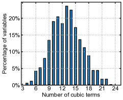
Figure 4: Distribution of the number of cubic terms with any variable.

For a general support of cubic interaction, we need $O(N^{3})$ couplers. However, for 3-SAT problems, the number of cubic terms is determined by the number of clauses $M$ which, for difficult problems, is typically about $4.2N$ [58]. This means that on average each variable is involved in about a dozen cubic terms – regardless of the size of the problem. Thus, we provide a fixed degree fan-in for cubic terms. As Fig. 4 shows, the distribution does not have a long tail. A fan-in degree $d=20$ would work for most benchmarks we studied. Given a fan-in limit chosen by a particular machine, users can pre-process excess clauses in a number of ways such as using the KZFD rule (Eq. 6).

Figure 5: High-level system overview of proposed cBRIM architecture demonstrating how baseline BRIM system can be extended to support cubic interaction.

The resulting architecture is shown in Fig. 5. We name this design, cubic BRIM or cBRIM in short. Every multiplier (AND gate) is fed by two $N$:1 multiplexers. This means that the cubic interactions encounter a small propagation delay relative to the quadratic interactions. Our simulation results show that, for our specific configuration, delays up to 3 ns are inconsequential for system performance.

IV-C3 Coupler programmability

Finally, another problem-specific feature of 3-SAT is that the vast majority of cubic term coefficients are $\pm 1$. For an $M$-clause 3-SAT problem, there are at most $M$ cubic terms produced by Eq. 4, one each by every clause with 3 literals. On rare occasions, different clauses may involve the same variables but with different negation patterns. Then, they either cancel out or add up to cubic coefficient of 2 or – at least in theory – even more. In such a case, that particular cubic term is simply treated as multiple instances that take up multiple couplers (fan-in). They just happen to select the same inputs for multiplication. So we eliminate the programmability on the coupler strength – it will be fixed at 1. Instead, the programmability is on which two inputs to multiply, and the polarity of the coupling.

Putting it together, a 3-SAT problem in CNF will be pre-processed via $O(3d_{max}\cdot M+N)$ time von Neumann computation (where $d_{max}$ is the maximum degree of the graph) to turn into a binary formulation (Eq. 8) organized as a matrix, and programmed into the hardware column by column. For linear and quadratic terms, the programmed values represent the coefficient of terms. For cubic terms, the programmed value identifies the variables to be multiplied together.

IV-D Annealing Control

A simple yet effective annealing control is to randomly flip a spin with a certain probability and gradually reduce this probability [3]. Motivated by observation 3 in Sec. III-C, we explore alternative control that can improve the hardware efficiency in navigating the landscape. In our 3-SAT solver architecture, there are at least two opportunities for improving navigational efficiency. ① First, we show that a completely random flipping strategy can lead to inefficiencies which motivates us to propose a novel semantic-aware random annealing in Sec. IV-D1. This requires us to compute a metric called make count ($\mathscr{M}_{n}$) discussed in Sec. IV-D2 and the hardware implementation details explained in Sec. IV-D3. ② Second, in Sec. IV-D4, we propose another optimization to stop annealing when ground state is identified.

IV-D1 Semantic-aware randomization

To understand the first opportunity, let us see why a baseline annealing control can be inefficient. Without any annealing control, the dynamical system simply evolves along trajectories determined by its differential equations. For our type of gradient system, this inevitably leads to (stable) fixed points [72]. Added random flips allow the system to break away from the original trajectory (Fig. 6). Because of its pure random nature, such a flip can lead the system to a different attraction region (red arrow ①) or merely to a different point inside the same attraction region (red arrow ②). While the former may lead to a more promising fixed point, the latter merely adds delay.

Figure 6: Illustration of landscape navigation by a dynamical system with annealing control. The horizontal axis shows all the phase point organized by their attraction region. The vertical axis shows each point’s energy. State change by system dynamics is shown in blue arrows, while red arrows show random spin flips. Note that in reality the neighboring relationship between attraction regions is far more complex in a high-dimension space than can be shown in a one-dimensional plot.

To make this navigation more efficient, we propose a new tanh-make-break (TMB) heuristic which assigns flip probability $p_{n}$ to each node $n$ as follows:

$$\begin{split}p_{n}=\tanh(c_{m}\times\mathscr{M}_{n})\cdot[1-\tanh(c_{b}\times\mathscr{B}_{n})]\end{split}$$ (10)

where $\mathscr{M}_{n}$ and $\mathscr{B}_{n}$ are the number of new clauses satisfied (make count) and unsatisfied (break count) respectively by flipping node $n$, and $c_{m}>0$ and $c_{b}>0$ are parameters. Our main motivation to use the $\tanh$ function are: ① easily implementable in hardware, ② directly resembles probability without any need for normalization, and ③ is non-linear as experimentally we found it to work better. Finding the most optimal function is left as future work. Thus, if a node has very high $\mathscr{M}_{n}$ compared to its $\mathscr{B}_{n}$, then it will have high chances of getting flipped. On the contrary, a node with relatively high $\mathscr{B}_{n}$ may be prohibited by the heuristic to flip. $c_{m}$ and $c_{b}$ determine how much weight to be assigned to $\mathscr{M}_{n}$ and $\mathscr{B}_{n}$. The main intuition is that, stochastically flipping nodes that satisfy more clauses makes the landscape navigation more efficient. We shall see later that with tuned $c_{m}$ and $c_{b}$ parameters, this indeed seems to be the case.

We use analog circuits to implement our TMB heuristic in hardware. In this regard, we need to compute $\mathscr{M}_{n}$ and $\mathscr{B}_{n}$ for each node. It turns out, the incoming current to each node is related to the difference ($\mathscr{M}_{n}-\mathscr{B}_{n}$) as shown below.

$$\begin{split}\frac{dv_{n}}{dt}&=\alpha(1-2x_{n})(\mathscr{M}_{n}-\mathscr{B}_{n})\end{split}$$ (11)

We omit the proof here to avoid the tedium. We opt to compute $\mathscr{M}_{n}$ since it is much easier to obtain and recover $\mathscr{B}_{n}$ from the incoming current in Eq. 11.

IV-D2 Computing $\mathscr{M}_{n}$

Let us consider the Hamiltonian ($H_{n}$) of only those clauses involving node $n$. This function has some terms that contain $v_{n}$ (we call them collectively $\mathscr{R}_{n}$) and the remaining that do not ($\mathscr{R}_{\char 92\relax n}$).

$$\begin{split}H_{n}&=const.-l_{n}v_{n}-\sum_{j}q_{nj}v_{n}v_{j}-\sum_{jk}c_{njk}v_{n}v_{j}v_{k}\\ &=\mathscr{R}_{n}+\mathscr{R}_{\char 92\relax n}=\mathscr{M}_{n}\end{split}$$ (12)

Now, $H_{n}$ is just the number of unsatisfied clauses associated with node $n$ and hence, is just $\mathscr{M}_{n}$. If we notice Eq. 9, the incoming current of each node is simply $\frac{dv_{n}}{dt}=-\alpha\partialderivative{\mathscr{R}_{n}}{v_{n}}$. This is because only $\mathscr{R}_{n}$ contains terms with $v_{n}$. Using this fact and applying Eq. 11 in Eq. 12,

$$\begin{split}\mathscr{M}_{n}&=H_{n}=x_{n}\partialderivative{\mathscr{R}_{n}}{v_{n}}+\mathscr{R}_{\char 92\relax n}\\ &=-\frac{x_{n}}{\alpha}\cdot\frac{dv_{n}}{dt}+\mathscr{R}_{\char 92\relax n}\\ &=x_{n}(\mathscr{M}_{n}-\mathscr{B}_{n})+\mathscr{R}_{\char 92\relax n}\end{split}$$ (13)

where $x_{n}$ is the quantized state of the node. While deriving Eq. 13, we use a simplification that since $x_{n}\in\{0,1\}$, we can write $x_{n}^{2}=x_{n}$. The first term in Eq. 13 can be obtained from the incoming current and only contributes when $x_{n}=1$. The second term ($\mathscr{R}_{\char 92\relax n}$) can be computed by generating a current with voltages of participating nodes applied across extra coupling units. As a result, we generate a current proportional to $\mathscr{M}_{n}$. With $\mathscr{M}_{n}$ computed, we can extract $\mathscr{B}_{n}$ using Eq. 11.

IV-D3 Hardware implementation

With $\mathscr{M}_{n}$ and $\mathscr{B}_{n}$ represented as currents, we can design a circuit to compute $p_{n}$ in Eq. 10 with approximate $\tanh$ generators and using an AND gate to approximate the multiplication. Fig. 7 shows an example implementation. The current $\mathscr{R}_{\char 92\relax n}$ is generated using coupling units not shown in the figure. Based on the quantized state of the node $x_{n}$, a switch is set to ensure the current flowing into the ($1-\tanh$) circuit is always $\mathscr{B}_{n}$ and also to get $\mathscr{M}_{n}$ from $\mathscr{R}_{\char 92\relax n}$. The $\tanh$ function is implemented by modifying a differential current-mode implementation shown in a recent work [22]. The resulting circuit is shown in Fig. 8. Using this, ($1-\tanh$) is trivial to implement as shown in the zoomed-in part of Fig. 7. The parameters $c_{m}$ and $c_{b}$ are tuned by applying a gain to the current-controlled current source that mirrors the input current in the $\tanh$ circuit. The output currents of the $\tanh$ and ($1-\tanh$) circuits, referred to as $I_{s}$ and $I_{t}$, are used to control the current-controlled voltage sources $V_{s}$ and $V_{t}$ respectively. Note that, $I_{s},I_{t}\in[0,I_{bias}]$ because the input currents, $\mathscr{M}_{n}$ and $\mathscr{B}_{n}$ are positive. $V_{s}$ and $V_{t}$ produce voltages in the range $[0,V_{DD}]$ which are fed as inputs to an AND gate to multiply approximately. The output of AND gate controls the probability $p_{n}$ of a stochastic circuit that outputs $V_{out}=1$ with a probability $p_{n}$. This way, each node can be selected by our TMB heuristic to flip if $V_{out}=1$.

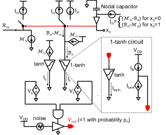
Figure 7: The CMOS circuit implementation of the heuristic.

Figure 8: CMOS implementation of a single-ended $\tanh$ circuit.

While the TMB heuristic requires extra hardware, it is only needed per node and thus comes with $O(N)$ cost. The system’s overall circuit complexity is dominated by that of the $O(N^{2})$ couplers in practical systems.

In a fast dynamical system like BRIM, flipping a node is a stochastic mechanism to escape local minima. It is done by “clamping” the node to a fixed polarity using a large current driver for a specific duration. Assuming the system started in a fixed point (local minimum), then after such a temporary clamp to a single node, the system will almost certainly revert back to the same fixed point. We need multiple clampings to overlap in order to escape.

By its very nature, our design flips nodes in an asynchronous manner and allows multiple stochastically overlapping flips. Lengthening the duration increases the number of overlaps. We will study the effect of the choice of clamp duration on the solution quality in Sec. V-C3.

IV-D4 Latching ground state

Another inefficiency is that the dynamical system has no explicit notion of energy the way a software algorithm does: it cannot determine whether one local minimum is better than another. In other words, software can always remember the phase point with the best energy ever visited, but a hardware solver can only read out the final state or at most a finite number of snapshots of the system’s trajectory. In a pure optimization task, this is an acceptable tradeoff in exchange for the extreme speed and efficiency. In SAT problems, the situation is a bit different. ① To solve the problem, we generally need to reach the ground state (though finding the maximum number of satisfiable clauses is useful too [50]). ② Unlike in many other problems (e.g., MaxCut), it is quite easy to know when the ground state is reached.

To sum, the risk-reward balance of a more explicit tracking of the energy value is shifted quite a bit in SAT. Thus we add an additional feature: when all clauses are satisfied, we simply stop adding any random flips and indicate the answer is found (latching). This is particularly convenient given our TMB heuristic: the formula is satisfied when $\mathscr{M}_{n}=0$ for all $N$ variables. As we will show in the analysis, this has a non-trivial boost to the effective speed of the machine.

V Experimental Analysis

V-A Experimental methodology

Most of the experiments are performed as a mixture of simulation and native execution. In all the experiments, CPU software solvers like WalkSAT[47] and KISSAT [18] are natively executed on Intel Xeon Platinum 8268 CPU at 2.90 GHz. WalkSAT is run using the -best heuristic also known as “SKC” [66] and a cutoff flips of 500,000. KISSAT is run using the default configuration. GPU-based solvers (ParaFrost [60] and AnalogSAT [55]) are run on an AMD Ryzen 5 2600 CPU at 3.4 GHz with 16 GB of 3200 MHz DDR4 RAM and an NVIDIA RTX 2070 Super GPU running at stock frequencies. The evolution of various dynamical systems is modeled by solving differential equations using 4th-order Runge-Kutta method. For a rough sense of the chip-based implementation, we perform a preliminary design and layout of components in Cadence using the generic 45nm PDK.

For SAT benchmarks, we use those publicly available from SATLIB [2] and SAT competitions. For direct comparison with other hardware solvers, we use the same publicly available problems. Moreover, we generate “hard” uniform random instances of varying sizes with $\alpha_{c}=4.25$. Majority of the hardware SAT solvers only test on uniform random problems [56, 38, 21] or tiny toy problems [11], however, it has been established that industrial problems exhibit scale-free behaviour [6, 7]. Therefore, we generated some difficult industrial-like SAT instances with 500 variables using scale-free distribution with $\alpha_{c}=3.29$ (1645 clauses) and power-law exponent of 2.8 [6].

V-B High-level analysis

We start with a high-level analysis comparing the architecture with all supports discussed in Sec. IV. We tuned the parameters $c_{m}$ and $c_{b}$ in our TMB heuristic that works the best, in general, for all problems. This augmented Ising machine for SAT (or AIMS for brevity) is first compared against state-of-the-art software solvers and cBRIM as defined in Sec. IV-C2. Note that, existing high order Ising machines have been either evaluated with tiny problems [11] or with poor solution quality and no direct report of the solver time [21]. In contrast, cBRIM is able to find solutions with higher success rates and hence, is compared here. Fig. 9 shows the Time-To-Solution (TTS) for all the solvers. The plot shows the geometric mean for each benchmark suite and also the overall TTS.

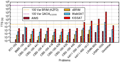
Figure 9: Time-To-Solution (s) of AIMS, cBRIM, WalkSAT and KISSAT for various benchmark suites from SATLIB and SAT 2011 competition. sat11 benchmark suites contain 4 problems each, both the LRAN benchmarks contain a single problem and the remaining benchmarks consist of 10 problems each. Each benchmark suite is named in this format: $\langle$Benchmark$\rangle$–$\langle$Vars$\rangle$–$\langle$Clauses (if stated)$\rangle$.

As we can see, for these benchmarks, AIMS is consistently faster with a geometric mean speedup about 2 and 3 orders of magnitude over software solvers WalkSAT [47] and KISSAT [18] respectively. With contributions from our TMB heuristic, AIMS outperforms cBRIM by at least an order of magnitude. Some of the data for cBRIM are missing as it could not solve the problems in our tested annealing times.

With the power consumption of AIMS estimated to be on the orders of 100 $mW$, energy consumption will likely be another order of magnitude better than von Neumann computing. The figure also shows the TTS of baseline BRIM using KZFD quadratization and an optimistic estimate of QAOA_ϵ/1000 on a 100-variable problem. Observe that AIMS is able to solve a 1000-variable problem while still being 2 orders of magnitude faster than baseline BRIM solving a 100-variable problem. Thus, we can see the importance of architectural design in AIMS to reach high problem solving capabilities. For the software solvers, except for the BMS instances, WalkSAT is able to outperform KISSAT. We do note that for much larger problems, the situation might be different as is evident from the SAT competitions [18]. The case for QAOA is not good as it is several orders of magnitude slower than even the software solvers.

Table I shows a comparison of AIMS with two other state-of-the-art hardware SAT solvers: HW AmoebaSAT [38] and BRWSAT [69]. The benchmarks shown here are the only ones reported by the references and hence, can be directly compared. Based only on the overlapping benchmarks, AIMS has a geometric speedup of 7.4x and 10.3x over HW AmoebaSAT and BRWSAT, respectively. Note that HW AmoebaSAT scales rather poorly as TTS increases 3 orders from problem sizes of 50 variables to 225 variables.

TABLE I: Comparison of TTS for various hardware solvers in units of $\mu s$. #V, #C: the number of variables and clauses, respectively.

Benchmark	#V	#C	HW AmoebaSAT	BRWSAT	AIMS
uf50-0100	$50$	$218$	$4.126$	$-$	$5.829$
uf50-0410	$50$	$218$	$4.360$	$-$	$1.329$
uf50-0767	$50$	$218$	$8.300$	$-$	$4.059$
uf100-0285	$100$	$430$	$356$	$-$	$73.81$
uf150-0100	$150$	$645$	$1832$	$-$	$73.16$
uf225-028	$225$	$960$	$3078$	$-$	$10.41$
sat11-350-p11	$350$	$1491$	$-$	$200$	$39.54$
sat11-350-p23	$350$	$1491$	$-$	$1289$	$44.56$
sat11-350-p75	$350$	$1491$	$-$	$280$	$22.81$
sat11-350-p98	$350$	$1491$	$-$	$50$	$7.389$
sat11-450-p1	$450$	$1917$	$-$	$80$	$6.448$
sat11-450-p11	$450$	$1917$	$-$	$1912$	$577.1$
sat11-450-p14	$450$	$1917$	$-$	$4650$	$786.2$
sat11-450-p78	$450$	$1917$	$-$	$353.1$	$8.082$

We also compare against GPU-based solvers. Fig. 10 shows the box plot distribution of TTS for AIMS compared with two state-of-the-art GPU-based SAT solvers: ParaFrost [60] and AnalogSAT [55]. The results of WalkSAT and KISSAT are also shown for reference. Each box expands from first quartile ($Q_{1}$) to third quartile ($Q_{3}$) of the results with a colored line at the median. The whiskers extend 1.5x of the inter-quartile distance ($Q_{3}-Q_{1}$) and the circle markers show outliers past the end of the whiskers.

Figure 10: Box plot showing distribution of TTS for AIMS, GPU-based solvers: ParaFrost and AnalogSAT, and software SAT solvers: WalkSAT and KISSAT. All solvers run 20 problems each with [Left] uniform random and [Right] industrial-like scale-free distribution of 500 variables.

We can observe that AIMS outperforms the better performing GPU-based solver, ParaFrost, by about 3 orders of magnitude for uniform random problem (left) and by 62x for industrial-like scale-free problems (right).

V-C In-depth analysis

V-C1 Navigational efficiency

First, we look at the navigational efficiency of AIMS. Fig. 11 shows the average number of phase points visited to reach SAT solution by AIMS and by cBRIM. Note here that the phase points visited is also adjusted by solution probability as in TTS (Eq. 7). AIMS is consistently more efficient than cBRIM as it could achieve a satisfying solution by visiting about 137x less phase points. Note again, in some benchmarks, cBRIM fails to find a solution, suggesting that it may require search through many more phase points. These benchmarks are not included here.

Figure 11: Phase points visited by AIMS and cBRIM for various benchmark suites from SATLIB and SAT competition.

V-C2 Impact of ground state latching

Next, we compare TTS with and without the result-latching logic discussed in Sec. IV-D4. Fig. 12 shows the best TTS AIMS can obtain with and without latching. We observe that with latching, the results are generally better as the system terminates immediately when a solution is found, rather than to run until the user defined cutoff time. On average, we find that with this logic, TTS improves by 1.9x compared to the best TTS obtained without latching. We note that beyond this speed improvement, the latch logic is likely to be of important practical value. It reduces the reliance on the user to set a judicious annealing time.

Figure 12: Results of AIMS with and without ground state latching.

V-C3 Relationship between clamp time and performance

Figure 13: [Left] Success probability (%) of AIMS while solving 20 instances of 500-variable problems with a cutoff time of 0.44 ms and increasing node clamp time. [Right] The number of heuristic and natural flips as node clamp time increases. The vertical red region shows the optimal clamp times.

In Sec. IV-D3, we discussed about asynchronous flips with node “clamping” which is the time until which a node’s voltage is held constant after a flip. Fig. 13 [Left] shows the success probability of AIMS while solving 20 instances of 500-variable problems with increasing node clamp time and constant annealing time of 0.44 ms. From the figure, we can observe that too short clamp times result in poor solution quality, most likely because the system did not get enough time to react to the flips. There are some optimal clamp times (shown by the “red” vertical region) resulting in the best success probability. Fig. 13 [Right] shows the number of flips done by our TMB heuristic and the “natural” flips done solely by the dynamical system. We notice that the amount of natural flips is very high for very short clamp time that results in poor solution quality. This number reduces as clamp time increases with the optimal region having roughly $10^{4}$ natural flips. The heuristic flips increases slightly after a rapid drop initially and are much higher than natural flips.

V-C4 Device variation and noise

We now analyze the effect of device variation on the performance of AIMS. The variations are obtained from Cadence by running a random Monte Carlo sampling in the Virtuoso Analog Design Environment XL. This sampling applies device mismatch and process variation, and is performed on a DC analysis by sweeping the input and measuring the output to obtain a transfer function. 1000 samples are taken for each circuit block, yielding 1000 curves relating the output to the input. These are then randomly sampled on a device-by-device basis in the behavioral model to estimate the impact on performance.

Figure 14: TTS of 3-SAT problems with different sizes for AIMS with ideal devices and devices with variation. Each size consist of 50 problems.

Fig. 14 shows the TTS of AIMS with ideal devices and devices with variation as problem size increases for both [left] uniform random and [right] scale-free distribution with power-law exponent 2.8. The cutoff times are set the same for both the ideal and device variation runs. We can make two key observations from the plots. First, there is a graceful degradation of performance and impact of device variation is still minimal for AIMS with a capacity of 500 nodes. Second, in the case of uniform random distribution, smaller problems (100 to 200 variables) performed better with device variation which implies that our TMB heuristic may be improved with further tuning.

Thermal noise analysis has only been performed on small scale systems of 50 nodes due to excessive simulation delays. A 3% Gaussian additive noise has no appreciable impact on performance. We note that unlike quantum computing, electronic Ising machines such as AIMS are much less susceptible to noise than quantum computers where noise fundamentally disrupts the working principle. For classical annealers, circuit noise may even be harnessed to help produce needed random perturbation in annealing.

VI Conclusions

With diminishing speed of improvements for conventional computing systems, non-von Neumann systems such as Ising machines are receiving increased attention. While all combinatorial optimization problems can be targeted by Ising machine in theory, we have shown in this paper, using SAT as a case study, that there are many practical hurdles with such systems: ① QUBO reduction of cubic terms in the SAT objective function creates significant search-space bloat; ② Problem-agnostic annealing leads to poor navigational efficiency relative to state-of-the-art software solvers.

Fortunately, these issues can be overcome with additional architectural support, at least for electronic Ising machines such as BRIM [3]. We have presented the design details to support cubic interaction natively in BRIM. More importantly, we have proposed a novel, semantic-aware annealing control along with a ground state latching mechanism. With the additional architectural support, the resulting augmented Ising machine for SAT (AIMS) can achieve orders of magnitude speedup over state-of-the-art SAT solvers.

Overall, our study suggests that Ising machines offer a powerful substrate to explore novel non-von Neumann computing. At the same time, additional architectural support may be crucial to truly unlock their performance potential.

References

- [1] “The international sat competition web page,” 2022. [Online]. Available: https://satcompetition.github.io/
- [2] “Satlib benchmarks,” 2022. [Online]. Available: https://www.cs.ubc.ca/~hoos/SATLIB/benchm.html
- [3] R. Afoakwa, Y. Zhang, U. K. R. Vengalam, Z. Ignjatovic, and M. Huang, “Brim: Bistable resistively-coupled ising machine,” 2021 IEEE International Symposium on High-Performance Computer Architecture (HPCA), pp. 749–760, 2021.
- [4] D. Aharonov, W. van Dam, J. Kempe, Z. Landau, S. Lloyd, and O. Regev, “Adiabatic quantum computation is equivalent to standard quantum computation,” arXiv, 2004. [Online]. Available: https://arxiv.org/abs/quant-ph/0405098
- [5] T. Albash and D. A. Lidar, “Adiabatic quantum computation,” Rev. Mod. Phys., vol. 90, p. 015002, Jan 2018. [Online]. Available: https://link.aps.org/doi/10.1103/RevModPhys.90.015002
- [6] C. Ansótegui, M. L. Bonet, and J. Levy, “On the structure of industrial sat instances,” in Principles and Practice of Constraint Programming-CP 2009: 15th International Conference, CP 2009 Lisbon, Portugal, September 20-24, 2009 Proceedings 15. Springer, 2009, pp. 127–141.
- [7] C. Ansótegui, M. L. Bonet, and J. Levy, “Towards industrial-like random sat instances,” in Proceedings of the 21st International Joint Conference on Artificial Intelligence, ser. IJCAI’09. San Francisco, CA, USA: Morgan Kaufmann Publishers Inc., 2009, p. 387–392.
- [8] M. Aono, M. Naruse, S.-J. Kim, M. Wakabayashi, H. Hori, M. Ohtsu, and M. Hara, “Amoeba-inspired nanoarchitectonic computing: Solving intractable computational problems using nanoscale photoexcitation transfer dynamics,” Langmuir : the ACS journal of surfaces and colloids, vol. 29, 04 2013.
- [9] A. Armando, R. Carbone, and L. Compagna, “Satmc: A sat-based model checker for security protocols, business processes, and security apis,” Int. J. Softw. Tools Technol. Transf., vol. 18, no. 2, p. 187–204, apr 2016. [Online]. Available: https://doi.org/10.1007/s10009-015-0385-y
- [10] A. Balint and U. Schöning, “Choosing probability distributions for stochastic local search and the role of make versus break,” in SAT, 2012.
- [11] M. K. Bashar, Z. Lin, and N. Shukla, “Oscillator-inspired dynamical systems to solve boolean satisfiability,” IEEE Journal on Exploratory Solid-State Computational Devices and Circuits, 2023.
- [12] M. K. Bashar, A. Mallick, A. W. Ghosh, and N. Shukla, “Dynamical system-based computational models for solving combinatorial optimization on hypergraphs,” IEEE Journal on Exploratory Solid-State Computational Devices and Circuits, 2023.
- [13] T. Baylo, M. J. Heule, M. Iser, M. Järvisalo, and M. Suda, “Proceedings of sat competition 2022 : Solver and benchmark descriptions,” in Proceedings of SAT Competition 2022 : Solver and Benchmark Descriptions, ser. Department of Computer Science Series of Publications B, vol. B-2022-1. Helsinki: Department of Computer Science, University of Helsinki, 2022. [Online]. Available: http://hdl.handle.net/10138/347211
- [14] K. Bharti, A. Cervera-Lierta, T. H. Kyaw, T. Haug, S. Alperin-Lea, A. Anand, M. Degroote, H. Heimonen, J. S. Kottmann, T. Menke, W.-K. Mok, S. Sim, L.-C. Kwek, and A. Aspuru-Guzik, “Noisy intermediate-scale quantum algorithms,” Rev. Mod. Phys., vol. 94, p. 015004, Feb 2022. [Online]. Available: https://link.aps.org/doi/10.1103/RevModPhys.94.015004
- [15] A. Biere, A. Cimatti, E. Clarke, M. Fujita, and Y. Zhu, “Symbolic model checking using sat procedures instead of bdds,” in Proceedings 1999 Design Automation Conference (Cat. No. 99CH36361), 1999, pp. 317–320.
- [16] A. Biere, M. Heule, H. van Maaren, and T. Walsh, Handbook of Satisfiability: Volume 185 Frontiers in Artificial Intelligence and Applications. NLD: IOS Press, 2009.
- [17] A. Biere, “Kissat,” 2022. [Online]. Available: https://github.com/arminbiere/kissat
- [18] A. Biere and M. Fleury, “Gimsatul, isasat, kissat entering the sat competition 2022,” in Proceedings of SAT Competition 2022 : Solver and Benchmark Descriptions, 2022.
- [19] F. Böhm, G. Verschaffelt, and G. Van der Sande, “A poor man’s coherent ising machine based on opto-electronic feedback systems for solving optimization problems,” Nature Communications, vol. 10, no. 1, p. 3538, 2019. [Online]. Available: https://doi.org/10.1038/s41467-019-11484-3
- [20] S. Boulebnane and A. Montanaro, “Solving boolean satisfiability problems with the quantum approximate optimization algorithm,” 2022. [Online]. Available: https://arxiv.org/abs/2208.06909
- [21] C. Bybee, D. Kleyko, D. E. Nikonov, A. Khosrowshahi, B. A. Olshausen, and F. T. Sommer, “Efficient optimization with higher-order ising machines,” arXiv preprint arXiv:2212.03426, 2022.
- [22] M. Carrasco-Robles and L. Serrano, “A novel cmos current mode fully differential tanh (x) implementation,” in 2008 IEEE International Symposium on Circuits and Systems (ISCAS), 2008, pp. 2158–2161.
- [23] D. A. Chermoshentsev, A. O. Malyshev, M. Esencan, E. S. Tiunov, D. Mendoza, A. Aspuru-Guzik, A. K. Fedorov, and A. I. Lvovsky, “Polynomial unconstrained binary optimisation inspired by optical simulation,” arXiv preprint arXiv:2106.13167, 2021.
- [24] V. Choi, “Adiabatic quantum algorithms for the np-complete maximum-weight independent set, exact cover and 3sat problems,” arXiv, April 2010.
- [25] V. Choi, “Different adiabatic quantum optimization algorithms for the NP-complete exact cover problem,” Proceedings of the National Academy of Sciences, vol. 108, no. 7, 2011. [Online]. Available: https://doi.org/10.1073%2Fpnas.1018310108
- [26] J. Coelho and M. Vanhoucke, “Multi-mode resource-constrained project scheduling using rcpsp and sat solvers,” European Journal of Operational Research, vol. 213, pp. 73–82, 08 2011.
- [27] S. A. Cook, “The complexity of theorem-proving procedures,” in Proceedings of the Third Annual ACM Symposium on Theory of Computing, ser. STOC ’71. New York, NY, USA: Association for Computing Machinery, 1971, p. 151–158. [Online]. Available: https://doi.org/10.1145/800157.805047
- [28] D-WAVE, “minorminer,” 2014. [Online]. Available: {https://github.com/dwavesystems/minorminer}
- [29] J. D. Davis, Z. Tan, F. Yu, and L. Zhang, “A practical reconfigurable hardware accelerator for boolean satisfiability solvers,” in Proceedings of the 45th Annual Design Automation Conference, ser. DAC ’08. New York, NY, USA: Association for Computing Machinery, 2008, p. 780–785. [Online]. Available: https://doi.org/10.1145/1391469.1391669
- [30] M. Davis, G. Logemann, and D. Loveland, “A machine program for theorem-proving,” Commun. ACM, vol. 5, no. 7, p. 394–397, jul 1962. [Online]. Available: https://doi.org/10.1145/368273.368557
- [31] V. Dunjko, Y. Ge, and J. I. Cirac, “Computational speedups using small quantum devices,” Physical Review Letters, vol. 121, no. 25, dec 2018. [Online]. Available: https://doi.org/10.1103%2Fphysrevlett.121.250501
- [32] E. Farhi, J. Goldstone, and S. Gutmann, “A quantum approximate optimization algorithm,” 2014. [Online]. Available: https://arxiv.org/abs/1411.4028
- [33] D. Freedman and P. Drineas, “Energy minimization via graph cuts: settling what is possible,” in 2005 IEEE Computer Society Conference on Computer Vision and Pattern Recognition (CVPR’05), vol. 2, 2005, pp. 939–946 vol. 2.
- [34] T. Gabor, S. Zielinski, S. Feld, C. Roch, C. Seidel, F. Neukart, I. Galter, W. Mauerer, and C. Linnhoff-Popien, “Assessing solution quality of 3sat on a quantum annealing platform,” 2019. [Online]. Available: https://arxiv.org/abs/1902.04703
- [35] L. K. Grover, “A fast quantum mechanical algorithm for database search,” in Proceedings of the twenty-eighth annual ACM symposium on Theory of computing, 1996, pp. 212–219.
- [36] K. Gulati, S. Paul, S. P. Khatri, S. Patil, and A. Jas, “Fpga-based hardware acceleration for boolean satisfiability,” ACM Trans. Des. Autom. Electron. Syst., vol. 14, no. 2, apr 2009. [Online]. Available: https://doi.org/10.1145/1497561.1497576
- [37] R. Hamerly, T. Inagaki, P. L. McMahon, D. Venturelli, A. Marandi, T. Onodera, E. Ng, C. Langrock, K. Inaba, T. Honjo, K. Enbutsu, T. Umeki, R. Kasahara, S. Utsunomiya, S. Kako, K. ichi Kawarabayashi, R. L. Byer, M. M. Fejer, H. Mabuchi, D. Englund, E. Rieffel, H. Takesue, and Y. Yamamoto, “Experimental investigation of performance differences between coherent ising machines and a quantum annealer,” Science Advances, vol. 5, no. 5, p. eaau0823, 2019. [Online]. Available: https://www.science.org/doi/abs/10.1126/sciadv.aau0823
- [38] K. Hara, N. Takeuchi, M. Aono, and Y. Hara-Azumi, “Amoeba-inspired stochastic hardware sat solver,” in 20th International Symposium on Quality Electronic Design (ISQED), 2019, pp. 151–156.
- [39] R. Harris, M. W. Johnson, T. Lanting, A. J. Berkley, J. Johansson, P. Bunyk, E. Tolkacheva, E. Ladizinsky, N. Ladizinsky, T. Oh, F. Cioata, I. Perminov, P. Spear, C. Enderud, C. Rich, S. Uchaikin, M. C. Thom, E. M. Chapple, J. Wang, B. Wilson, M. H. S. Amin, N. Dickson, K. Karimi, B. Macready, C. J. S. Truncik, and G. Rose, “Experimental investigation of an eight-qubit unit cell in a superconducting optimization processor,” Phys. Rev. B, vol. 82, p. 024511, Jul 2010.
- [40] T. Honjo, T. Sonobe, K. Inaba, T. Inagaki, T. Ikuta, Y. Yamada, T. Kazama, K. Enbutsu, T. Umeki, R. Kasahara, K. ichi Kawarabayashi, and H. Takesue, “100,000-spin coherent ising machine,” Science Advances, vol. 7, no. 40, p. eabh0952, 2021. [Online]. Available: https://www.science.org/doi/abs/10.1126/sciadv.abh0952
- [41] T. Inagaki, Y. Haribara, K. Igarashi, T. Sonobe, S. Tamate, T. Honjo, A. Marandi, P. L. McMahon, T. Umeki, K. Enbutsu, O. Tadanaga, H. Takenouchi, K. Aihara, K.-i. Kawarabayashi, K. Inoue, S. Utsunomiya, and H. Takesue, “A coherent ising machine for 2000-node optimization problems,” Science, vol. 354, no. 6312, pp. 603–606, 2016. [Online]. Available: https://science.sciencemag.org/content/354/6312/603
- [42] S. Isakov, I. Zintchenko, T. Rønnow, and M. Troyer, “Optimised simulated annealing for ising spin glasses,” Computer Physics Communications, vol. 192, p. 265–271, Jul 2015. [Online]. Available: http://dx.doi.org/10.1016/j.cpc.2015.02.015
- [43] F. Ivančić, Z. Yang, M. K. Ganai, A. Gupta, and P. Ashar, “Efficient sat-based bounded model checking for software verification,” Theor. Comput. Sci., vol. 404, no. 3, p. 256–274, sep 2008. [Online]. Available: https://doi.org/10.1016/j.tcs.2008.03.013
- [44] K. Jun and H. Lee, “Hubo formulations for solving the eigenvalue problem,” Results in Control and Optimization, p. 100222, 2023.
- [45] T. Kadowaki and H. Nishimori, “Quantum annealing in the transverse ising model,” Physical Review E, vol. 58, no. 5, pp. 5355–5363, nov 1998. [Online]. Available: https://doi.org/10.1103%2Fphysreve.58.5355
- [46] T. Kanao and H. Goto, “Simulated bifurcation for higher-order cost functions,” Applied Physics Express, vol. 16, no. 1, p. 014501, 2022.
- [47] H. Kautz, “Walksat,” 2018. [Online]. Available: https://gitlab.com/HenryKautz/Walksat
- [48] S. Kirkpatrick, C. D. Gelatt Jr, and M. P. Vecchi, “Optimization by simulated annealing,” science, vol. 220, no. 4598, pp. 671–680, 1983.
- [49] V. Kolmogorov and R. Zabin, “What energy functions can be minimized via graph cuts?” IEEE Transactions on Pattern Analysis and Machine Intelligence, vol. 26, no. 2, pp. 147–159, 2004.
- [50] M. Koshimura, T. Zhang, H. Fujita, and R. Hasegawa, “Qmaxsat: A partial max-sat solver,” Journal on Satisfiability, Boolean Modeling and Computation, vol. 8, no. 1-2, pp. 95–100, 2012.
- [51] W. Liu, Z. Gu, and Y. Ye, “Efficient sat-based application mapping and scheduling on multiprocessor systems for throughput maximization,” in 2015 International Conference on Compilers, Architecture and Synthesis for Embedded Systems (CASES), 2015, pp. 127–136.
- [52] A. Lucas, “Ising formulations of many np problems,” Frontiers in Physics, vol. 2, p. 5, 2014.
- [53] J. Marques Silva and K. Sakallah, “Grasp-a new search algorithm for satisfiability,” in Proceedings of International Conference on Computer Aided Design, 1996, pp. 220–227.
- [54] P. L. McMahon, A. Marandi, Y. Haribara, R. Hamerly, C. Langrock, S. Tamate, T. Inagaki, H. Takesue, S. Utsunomiya, K. Aihara, R. L. Byer, M. M. Fejer, H. Mabuchi, and Y. Yamamoto, “A fully programmable 100-spin coherent ising machine with all-to-all connections,” Science, vol. 354, no. 6312, pp. 614–617, 2016. [Online]. Available: https://science.sciencemag.org/content/354/6312/614
- [55] F. Molnár, S. R. Kharel, X. S. Hu, and Z. Toroczkai, “Accelerating a continuous-time analog sat solver using gpus,” Computer Physics Communications, vol. 256, p. 107469, 2020. [Online]. Available: https://www.sciencedirect.com/science/article/pii/S0010465520302204
- [56] A. H. N. Nguyen, M. Aono, and Y. Hara-Azumi, “Amoeba-inspired hardware sat solver with effective feedback control,” in 2019 International Conference on Field-Programmable Technology (ICFPT), 2019, pp. 243–246.
- [57] A. Niewiadomski, P. Switalski, T. Sidoruk, and W. Penczek, “Applying modern sat-solvers to solving hard problems,” Fundam. Informaticae, vol. 165, pp. 321–344, 2019.
- [58] H. Nishimori, Statistical Physics of Spin Glasses and Information Processing. Oxford University Press, 2001.
- [59] M. Norimoto, R. Mori, and N. Ishikawa, “Quantum algorithm for higher-order unconstrained binary optimization and mimo maximum likelihood detection,” IEEE Transactions on Communications, 2023.
- [60] M. Osama, A. Wijs, and A. Biere, “Sat solving with gpu accelerated inprocessing,” in Tools and Algorithms for the Construction and Analysis of Systems: 27th International Conference, TACAS 2021, Held as Part of the European Joint Conferences on Theory and Practice of Software, ETAPS 2021, Luxembourg City, Luxembourg, March 27–April 1, 2021, Proceedings, Part I 27. Springer, 2021, pp. 133–151.
- [61] E. Pelofske, G. Hahn, and H. Djidjev, “Optimizing the spin reversal transform on the d-wave 2000q,” in 2019 IEEE International Conference on Rebooting Computing (ICRC), 2019, pp. 1–8.
- [62] I. G. Rosenberg, “Reduction of bivalent maximization to the quadratic case,” Cahiers du Centre d’Etudes de Recherche Operationnelle, vol. 17, pp. 71–74, 1975.
- [63] D. Scheder and J. P. Steinberger, “Ppsz for general k-sat: Making hertli’s analysis simpler and 3-sat faster,” in Proceedings of the 32nd Computational Complexity Conference, ser. CCC ’17. Dagstuhl, DEU: Schloss Dagstuhl–Leibniz-Zentrum fuer Informatik, 2017.
- [64] T. Schoning, “A probabilistic algorithm for k-sat and constraint satisfaction problems,” in 40th Annual Symposium on Foundations of Computer Science (Cat. No.99CB37039), 1999, pp. 410–414.
- [65] D. Schreiber, “Lilotane: A lifted sat-based approach to hierarchical planning,” J. Artif. Int. Res., vol. 70, p. 1117–1181, may 2021. [Online]. Available: https://doi.org/10.1613/jair.1.12520
- [66] B. Selman, H. A. Kautz, B. Cohen et al., “Local search strategies for satisfiability testing.” Cliques, coloring, and satisfiability, vol. 26, pp. 521–532, 1993.
- [67] A. Sharma, R. Afoakwa, Z. Ignjatovic, and M. Huang, “Increasing ising machine capacity with multi-chip architectures,” in Proceedings of the 49th Annual International Symposium on Computer Architecture, ser. ISCA ’22. New York, NY, USA: Association for Computing Machinery, 2022, p. 508–521. [Online]. Available: https://doi.org/10.1145/3470496.3527414
- [68] Y. Shen, A. Rezaei, and H. Zhou, “Sat-based bit-flipping attack on logic encryptions,” in 2018 Design, Automation & Test in Europe Conference & Exhibition (DATE), 2018, pp. 629–632.
- [69] Y. Shim, A. Sengupta, and K. Roy, “Biased random walk using stochastic switching of nanomagnets: Application to sat solver,” IEEE Transactions on Electron Devices, vol. 65, no. 4, pp. 1617–1624, 2018.
- [70] P. W. Shor, “Polynomial-time algorithms for prime factorization and discrete logarithms on a quantum computer,” SIAM Journal on Computing, vol. 26, no. 5, pp. 1484–1509, oct 1997. [Online]. Available: https://doi.org/10.1137%2Fs0097539795293172
- [71] A. A. Sohanghpurwala, M. W. Hassan, and P. M. Athanas, “Hardware accelerated sat solvers - a survey,” J. Parallel Distributed Comput., vol. 106, pp. 170–184, 2017.
- [72] S. Strogatz, “Nonlinear dynamics and chaos: With applications to physics, biology, chemistry and engineering (cambridge, ma: Westview),” Book, 1994.
- [73] J. Su, T. Tu, and L. He, “A quantum annealing approach for boolean satisfiability problem,” in Proceedings of the 53rd Annual Design Automation Conference, 2016, pp. 1–6.
- [74] K. Takata, A. Marandi, R. Hamerly, Y. Haribara, D. Maruo, S. Tamate, H. Sakaguchi, S. Utsunomiya, and Y. Yamamoto, “A 16-bit coherent ising machine for one-dimensional ring and cubic graph problems,” Scientific Reports, vol. 6, no. 1, p. 34089, 2016. [Online]. Available: https://doi.org/10.1038/srep34089
- [75] S. Tan, M. Yu, A. Python, Y. Shang, T. Li, L. Lu, and J. Yin, “Hyqsat: A hybrid approach for 3-sat problems by integrating quantum annealer with cdcl,” in 2023 IEEE International Symposium on High-Performance Computer Architecture (HPCA). IEEE, 2023, pp. 731–744.
- [76] S. Tari, S. Verel, and M. Omidvar, “Pubo i: A tunable benchmark with variable importance,” in Evolutionary Computation in Combinatorial Optimization: 22nd European Conference, EvoCOP 2022, Held as Part of EvoStar 2022, Madrid, Spain, April 20–22, 2022, Proceedings. Springer, 2022, pp. 175–190.
- [77] K. Tatsumura, A. R. Dixon, and H. Goto, “Fpga-based simulated bifurcation machine,” in 2019 29th International Conference on Field Programmable Logic and Applications (FPL), 2019, pp. 59–66.
- [78] G. S. Tseitin, On the Complexity of Derivation in Propositional Calculus. Berlin, Heidelberg: Springer Berlin Heidelberg, 1983, pp. 466–483. [Online]. Available: https://doi.org/10.1007/978-3-642-81955-1_28
- [79] T. Wang and J. Roychowdhury, “OIM: oscillator-based ising machines for solving combinatorial optimisation problems,” CoRR, vol. abs/1903.07163, 2019. [Online]. Available: http://arxiv.org/abs/1903.07163
- [80] T. Wang, L. Wu, and J. Roychowdhury, “New computational results and hardware prototypes for oscillator-based ising machines,” in Proceedings of the 56th Annual Design Automation Conference 2019, ser. DAC ’19. New York, NY, USA: Association for Computing Machinery, 2019. [Online]. Available: https://doi.org/10.1145/3316781.3322473
- [81] Y. Wang and P. S. Krstic, “Prospect of using grover's search in the noisy-intermediate-scale quantum-computer era,” Physical Review A, vol. 102, no. 4, oct 2020. [Online]. Available: https://doi.org/10.1103%2Fphysreva.102.042609
- [82] K. Yamamoto, K. Kawamura, K. Ando, N. Mertig, T. Takemoto, M. Yamaoka, H. Teramoto, A. Sakai, S. Takamaeda-Yamazaki, and M. Motomura, “Statica: A 512-spin 0.25m-weight annealing processor with an all-spin-updates-at-once architecture for combinatorial optimization with complete spin–spin interactions,” IEEE Journal of Solid-State Circuits, vol. 56, no. 1, pp. 165–178, 2021.
- [83] Y. Yamamoto, K. Aihara, T. Leleu, K.-i. Kawarabayashi, S. Kako, M. Fejer, K. Inoue, and H. Takesue, “Coherent ising machines—optical neural networks operating at the quantum limit,” npj Quantum Information, vol. 3, no. 1, p. 49, 2017. [Online]. Available: https://doi.org/10.1038/s41534-017-0048-9
- [84] H. Zhou, R. Jiang, and S. Kong, “Cycsat: Sat-based attack on cyclic logic encryptions,” in 2017 IEEE/ACM International Conference on Computer-Aided Design (ICCAD), 2017, pp. 49–56.