Simple Computation of the MultiExp Gaussian Quadrature in Double Precision

Abstract

The MultiExp Gaussian quadrature rule proposed by Gill and Chien has many compelling properties for the integration of radial integrands encountered in electronic structure, but thus far has only been computed up to $N=50$, with some nontrivial holes in the existing tables for $27\leq N<50$. In this work, a simple recipe is developed to compute the MultiExp Gaussian quadrature for larger $N$ at close to the double precision machine epsilon. Notably, this recipe uses only double precision operations, so no computer algebra systems or arbitrary precision libraries are needed. There are three primary outcomes: (A) The MultiExp tables for all $N\leq 1000$ are presented in a supplement to this report - these might prove useful in building better medium and high quality density functional theory quadrature grids (B) these tables are compared to the known Gill and Chien tables with excellent agreement obtained modulo a noticeable problem with the weights of the largest $N=50$ Gill and Chien table and (C) it may be the case that the Boley-Golub plus extremely high-order Gauss-Legendre quadrature approximation recipe developed in this work could be used to automatically derive other quadrature rules throughout electronic structure theory and beyond.

I Introduction

The efficient quadrature-based integration of complicated integrands in the radial coordinate of the form $I\equiv\int_{0}^{\infty}\mathrm{d}r\ r^{2}f(r)\approx\sum_{i}u_{i}f(r_{i})$ is a crucial task in molecular electronic structure theory. As just one example, this is a key step in the “molecule-shaped” integration of the nonlinear Kohn-Sham exchange-correlation potential over of density functional theory. Moreover, this step seems to have more heuristic choice involved than the other steps. Molecular quadratures of the Becke polyatomic grid typeBecke (1988) can usually be thought of in terms of three steps: (1) atomic partitioning, (2) solid angle integration, and (3) radial integration. Despite a fair amount of high-quality work on (1), the widely prevailing sentiment is that Becke’s original choiceBecke (1988) of a thrice-iterated smooth cubic cutoff function in confocal elliptic coordinates provides a heuristically optimal smooth Voronoi tessellation of the molecule for this consideration (note that a small “bump-function” modification of this procedure by Stratmann, Scuseria, and FrischStratmann et al. (1996) achieves essentially the same quality of partition function, albeit with the possibility of strict linear scaling computation). (2) involves integration of medium-order spherical harmonics over the solid angle, with a strong desire to preserve at least octahedral symmetry, leading to Lebedev-Laikov gridsLebedev (1976); Lebedev and Laikov (1999) as the widely prevailing choice.

For (3), many proposals have been made: “classic” Gauss-Laguerre, Becke,Becke (1988) Handy,Murray et al. (1993) Ahlrichs,Treutler and Ahlrichs (1995) Knowles,Mura and Knowles (1996) Mitani and Yoshioka’s double exponential,Mitani and Yoshioka (2012) and Shizgal et al’s Gauss-Maxwell,Shizgal et al. (2017) among others, and all of these seem to have their own pros and cons, e.g., there is seemingly no clear choice of a universal radial quadrature rule. However, there is one more radial quadrature rule that is highly compelling: the multi-exponential or “MultiExp” quadrature of Gill and Chien.Gill and Chien (2003) The MultiExp quadrature starts from the “log-squared” Gaussian quadrature rule for the unique $N$-node grid of points and weights $\{<x_{i},w_{i}>\}$ that exactly integrate polynomials of order $2N-1$ over $x\in[0,1]$ when multiplied by the weight function $\ln^{2}(x)$, i.e.,

$$\int_{0}^{1}\mathrm{d}x\ \ln^{2}(x)f(x)=\sum_{i=1}^{N}w_{i}f(x_{i})\ \forall\ f(x)\in\mathcal{P}_{2N-1}(x)$$ (1)

The log-squared quadrature rules for $N\leq 100$ are depicted in Fig. 1 - the precise determination of the log-squared quadratures up to $N=1000$ is the primary outcome of the present work.

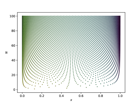
Figure 1: Visual representation of the finished log-squared quadrature grids for $1\leq N\leq 100$ obtained in this work. The colors represent the logarithms of the weights, with $10^{0}$ appearing as yellow and $10^{-6}$ appearing as purple. Some weights exceed this range and are clamped to the endpoint colors.

With an “atomic size” parameter $R$, the transformation,

$$r_{i}\equiv-R\ln(x_{i})$$ (2)

and,

$$u_{i}\equiv R^{3}\frac{w_{i}}{x_{i}}$$ (3)

yields the desired radial MultiExp quadrature rule,

$$\int_{0}^{\infty}\mathrm{d}r\ r^{2}f(r)\approx\sum_{i=1}^{N}u_{i}f(r_{i})$$ (4)

Just as the log-squared quadrature is exact for polynomials in $x$ integrands multiplied by $\ln^{2}(x)$, the MultiExp radial quadrature grid is exact for integrands in $r$ multiplied by $r^{2}$ of the “multi-exponential” form,

$$f(r)=\sum_{k=1}^{2N}a_{k}\exp(-kr/R)\ \forall\ \{a_{k}\}\in\mathbb{R}^{2N}$$ (5)

This multi-exponential form is heuristically well-suited to radial integrands involving the electronic density that are commonly encountered in electronic structure theory. In practice, the MultiExp quadratures perform remarkably well for density-involving integrands, e.g., forming the basis for the “good-for-the-money” SG-0 gridChien and Gill (2006) that is widely used in electronic structure.

One major barrier to further adoption of the MultiExp quadrature is that the accurate computation of the quadrature rules appears to be exceedingly difficult with standard techniques. Gill has tabulated the rules to 15 absolute decimal digits for $N\in\{1,\ldots,26,30,35,40,45,50\}$ on his research group’s website,Gill and Chien and these specific rules are widely available in open-source and proprietary electronic structure codes. In the Gill and Chien MultiExp paper,Gill and Chien (2003) the recipe to determine these weights is stated as “[B]y inverting the Cholesky triangle of the associated Gram matrix, we have constructed the $Q_{n}(x)$ [the orthogonal polynomials for $\ln^{2}(x)$] for $1\leq n\leq 27$. The associated roots and weights … are listed in Table 1.” This together with the integral example definition of $Q_{0}(x)=1$, $Q_{1}(x)=8x-1$, $Q_{2}(x)=7992x^{2}-4104x+217$ (neither monic nor normalized) provided in a footnote suggest that an integer coefficient computer algebra system for polynomials was used to derive the explicit form of the orthogonal polynomials. The roots of these polynomials and weights (related to the derivative of the polynomial at each root) were then likely extracted by an arbitrary-precision numerical procedure to obtain the tabulated quadratures to near double-precision accuracy. Note that exact integer representation of a family of orthogonal polynomials is often considered to be a last resort, as the required RAM and compute time to store and manipulate the integer coefficients may grow exponentially with order. It is quite impressive that this approach has already made it out to $N=45$ or $N=50$. (However, the present work indicates there may be a non-trivial problem with the grid Gill and Chien report for $N=50$, see below).

In this work we will (1) describe a simple recipe to compute the MultiExp quadrature rules to close to the double precision machine epsilon using only double precision computation and (2) present the MultiExp roots and weights for $N\leq 1000$. Note that below, we prefer to define the log-squared Gaussian quadrature as the MultiExp quadrature - the context of integrating in $x$ or $r$ will resolve this nuance in the notation.

II Theory

II.1 The Boley-Golub Algorithm

The starting point for our method is the Boley-Golub algorithmBoley and Golub (1987) to transform a quadrature rule (Gaussian or not) in one measure to a true Gaussian quadrature rule in a different measure. An additional explanatory reference on the Boley-Golub algorithm is as follows.Fernandes and Atchley (2006)

We seek the $N$-point Gaussian quadrature rule $\{<x_{i},w_{i}>\}$ for integration over $x$ from $a$ to $b$ with weight function $\mu(x)$,

$$\int_{a}^{b}\mathrm{d}x\ \mu(x)f(x)=\sum_{i=1}^{N}w_{i}f(x_{i}):\ f(x)\in\mathcal{P}_{2N-1}(x)$$ (6)

Let us say we have another set of $Q$-point quadrature rules $\{<\xi_{i},q_{i}>\}$ for the measure integral,

$$\int_{a}^{b}\mathrm{d}x\ \mu(x)\approx\sum_{i=1}^{Q}q_{i}\mu(\xi_{i})$$ (8)

Now we can construct the $Q+1$-dimensional square symmetric matrix,

$$\hat{W}\equiv\left[\begin{array}[]{r|rrrr}1&\sqrt{\omega_{0}}&\sqrt{\omega_{1}}&\sqrt{\omega_{2}}&\ldots\\ \hline\cr\sqrt{\omega_{0}}&\xi_{0}&0&0&\ldots\\ \sqrt{\omega_{1}}&0&\xi_{1}&0&\ldots\\ \sqrt{\omega_{2}}&0&0&\xi_{2}&\ldots\\ \vdots&\vdots&\vdots&\vdots&\ddots\\ \end{array}\right]:\ \sqrt{\omega_{i}}\equiv\sqrt{q_{i}\mu(\xi_{i})}$$ (9)

This orthogonally tridiagonalizes in the large $Q$ limit via,

$$\hat{T}=\hat{Q}^{\dagger}\hat{T}\hat{Q}:\ \hat{Q}\hat{Q}^{\dagger}=\hat{I}$$ (10)

to,

$$\hat{T}\equiv\left[\begin{array}[]{r|rrrr}1&\sqrt{b_{0}}&0&0&\ldots\\ \hline\cr\sqrt{b_{0}}&d_{0}&\sqrt{b_{1}}&0&\ldots\\ 0&\sqrt{b_{1}}&d_{1}&\sqrt{b_{2}}&\ldots\\ 0&0&\sqrt{b_{2}}&d_{2}&\ldots\\ \vdots&\vdots&\vdots&\vdots&\ddots\\ \end{array}\right]\equiv\left[\begin{array}[]{r|r}1&\vec{c}_{0}^{\dagger}\\ \hline\cr\vec{c}_{0}&\hat{J}\\ \end{array}\right]$$ (11)

Note that for our purposes, the phases of the tridiagonalization can be canonicalized by requiring that the superdiagonal elements all be positive.

The second full minor $\hat{J}$ is the Golub-Welsch Jacobian matrix. The entry $T_{1,0}$ is $\sqrt{b_{0}}$, the square root of the zeroth moment,

$$b_{0}=\int_{a}^{b}\mathrm{d}x\ \mu(x)$$ (12)

II.2 The Golub-Welsch Algorithm

As soon as $N+1$ rows and columns of $\hat{T}$ are uncoupled in the tridiagonalization procedure, the symmetric, tridiagonal Golub-Welsch Jacobian matrix $\hat{J}_{(N)}$ is available, i.e., full tridiagonalization of $\hat{T}$ is not required for $N<Q$.

At this point, we turn to the famous Golub-Welsch algorithm,Golub and Welsch (1969) which is succinctly stated as follows: Diagonalize the symmetric, tridiagonal Golub-Welsch Jacobian matrix,

$$\hat{J}_{(N)}=\hat{U}_{(N)}\hat{x}^{(N)}\hat{U}_{(N)}^{\dagger}$$ (13)

and obtain the $N$-node Gaussian quadrature roots as the eigenvalues of $\hat{J}_{(N)}$, i.e., $\{x_{i}\}=\hat{x}^{(N)}$. The corresponding Gaussian quadrature weights are obtained from the first row of the eigenvectors as,

$$w_{i}=b_{0}\left(\hat{U}_{(N)}[0,i]\right)^{2}\forall\ i\in 1\ldots N$$ (14)

II.3 Accuracy Considerations

Stability: The orthogonal tridiagonalization procedure of the Boley-Golub algorithm and the diagonalization of the Golub-Welsch algorithm both involve orthogonal transforms that are typically found to be stable and precise to a few ulp. Specifically, we use a standard system LAPACK DSYEV call for the needed eigenvalues and eigenvectors in Golub-Welsch (it is relatively easy to reduce the Golub-Welsch diagonalization computational effort by exploiting the fact that $\hat{J}_{(N)}$ is already tridiagonal to achieve linear scaling in this step, but this is overkill for the $N\leq 1000$ we will be considering within this work). For the partial tridiagonalization step of the Boley-Golub algorithm, we use a handwritten algorithm using Householder reflectors, with the only unusual concession to numerical stability being the use of Kahan-Babushka-Klein summationKahan (1965); Klein (2006) in the very long dot products of size $Q$. With these considerations, Boley-Golub + Golub-Welsch can be considered to be precise up to a few ulp in double precision.

Accuracy: With stability out of the way, we now consider the primary numerical consideration of the full procedure: accuracy. The only formal approximation made in the whole procedure above is that the $Q$-point quadrature rule $\{<\xi_{i},q_{i}>\}$ used in Boley-Golub is an approximate quadrature rule for the target metric integral. In formal practice, the accuracy of the overall $N$-node procedure is governed by the accuracy of resolving the set of $2N$ moments,

$$M^{(k)}\equiv\int_{a}^{b}\mathrm{d}x\ \mu(x)x^{k}\approx\sum_{i=1}^{Q}q_{i}\mu(\xi_{i})\xi_{i}^{k}\ \forall\ k\in[0,2N-1]$$ (15)

The reason for this is that the Golub-Welsch Jacobi matrix is formally completely defined by the lowest $2N$ moments $M^{(k)}$. However, we typically eschew explicit manipulations of high-order moments in numerical practice due to atrocious stability considerations, e.g., we use a Boley-Golub-construction of the Golub-Welsch Jacobian rather than a moment-based construction. In our specific prescription below, we will find that $M^{(0)}=b_{0}$ converges dramatically more slowly with $Q$ than the other moments, and thus the accuracy in $M^{(0)}$ can be used as a rough yardstick for the quality of our $Q$-point Boley-Golub approximation that is seemingly independent of $N$.

Accuracy Special Case: One special case is worth talking about: A $Q\geq N$-point Gaussian quadrature rule for the weight function $\mu(x)$ definitionally exactly integrates all of the lowest $2Q\geq 2N$ moments, and therefore will yield an exact Boley-Golub + Golub-Welsch procedure (note that there is a minor detail that the weight function is already built into the Gaussian quadrature weights, so we must substitute $\sqrt{\omega_{i}}\equiv\sqrt{w_{i}}$ for this case). This seems at first glance to be begging the question - we are saying that a Gaussian quadrature is a great way to discover the same or smaller Gaussian quadratures. But it turns out to be very useful to help validate a proposed grid: running Boley-Golub + Golub-Welsch from a proposed highly-accurate $Q$-point Gaussian quadrature rule should reproduce all $N\leq Q$ Gaussian quadrature rules to nearly the machine epsilon, and any deviation from this behavior is indicative of a serious problem with the proposed $Q$-point Gaussian quadrature.

II.4 High-Order Gauss-Legendre Quadrature

To close the procedure and compute the MultiExp quadrature, all that remains is to find an accurate arbitrary $Q$-node quadrature rule $\{<\xi_{i},q_{i}>\}$ for the specific MultiExp moments,

$$M^{(k)}\equiv\int_{0}^{1}\mathrm{d}x\ \ln^{2}(x)x^{k}\approx\sum_{i=1}^{Q}q_{i}\ln^{2}(\xi_{i})\xi_{i}^{k}=\frac{2}{(k+1)^{3}}$$ (16)

These are a numerical bear: $k=0$ is plagued by the log-squared pole at $x=0$, while for $k>0$ the pole is extinguished and increasingly higher effort is required for the transients that gradually emerge in the middle of the integration domain. There are seemingly very few general-purpose quadrature rules that can handle this behavior. Indeed, this may be the reason MultiExp is so compelling - it is the quadrature rule that handles this behavior.

After many failed attempts, we have found that extremely high-order Gauss-Legendre quadrature rules can crack the problem. The “classic” $Q$-node Gauss-Legendre quadrature rule is $\{<x_{i},w_{i}>\}$ where,

$$\int_{-1}^{+1}\mathrm{d}x\ f(x)=\sum_{i=1}^{Q}w_{i}f(x_{i})\ \forall\ f(x)\in\mathcal{P}_{2Q-1}(x)$$ (17)

We can then substitute this into our Boley-Golub + Golub-Welsch procedure via,

$$\xi_{i}\equiv\frac{1}{2}[x_{i}+1],\ q_{i}\equiv\frac{1}{2}w_{i}$$ (18)

$$\sqrt{\omega_{i}}\equiv\sqrt{q_{i}}|\ln(\xi_{i})|$$ (19)

For reasons discussed momentarily, we actually prefer to substitute a nonlinear remapping of the interval, for some paramter $\gamma$,

$$\xi_{i}^{\prime}\equiv\xi_{i}^{\gamma},\ q_{i}^{\prime}\equiv\gamma\xi_{i}^{\gamma-1}q_{i}$$ (20)

With $\gamma=1$ (no nonlinear remapping), we find that the moments converge slowly but regularly, with $M^{(0)}$ dramatically dominating the convergence behavior presumably due to the log-squared pole at $x=0$ for $k=0$. We have managed to converge the MultiExp quadrature for $N\leq 100$ to almost the double machine precision with $\gamma=1$, but this requires an extremely high cost of $Q\sim 2\times 10^{8}$. Using $\gamma=2$ quadratically clusters more of the Gauss-Legendre points near the difficult $x=0$ portion of the interval without significantly compromising the sampling near $x=1$. We find that this dramatically increases the convergence rate of the lower moments without compromising the stability of the overall approach, e.g., allowing for double precision convergence to be obtained by $Q\sim 10^{5}$. Unless otherwise specified, all results below use $\gamma=2$.

The last step needed to close the procedure is to obtain a recipe to efficiently obtain the $Q$-node Gauss-Legendre quadrature rule $\{<x_{i},w_{i}>\}$ to very close to the double machine precision. Thanks to the excellent 2014 work of Bogaert,Bogaert (2014) this is a solved problem. Bogaert’s paper provides an explicit, stable, non-iterative double-precision recipe to compute the Gauss-Legendre quadrature nodes and weights to the double machine precision using only standard scalar math library functions. This procedure can be implemented in an afternoon using $<200$ lines of C++ using only the standard library. An entertaining “race report” on the highly interesting topic of high-order Gauss-Legendre quadratures is provided by Townsend.Townsend (2015)

III Implementation

A simple C++ implementation of the above procedure was developed in the proprietary QC Ware Tachyon electronic structure library. Bogaert’s fast asymptotic Gauss-Legendre quadrature method was implemented from scratch in a way that essentially mirrors Bogaerts paper, albeit that we find Chebyshev conditioning of the $F$ and $W$ intermediates to not be required if the lower-half of the Gauss-Legendre nodes are explicitly computed and then the upper-half of the Gauss-Legendre nodes (which are less accurate) are obtained by symmetry. As with Bogaert, we believe that the Gauss-Legendre quadrature rules computed with this rule are accurate to a few ulp. A partial Householder tridiagonalization subroutine was developed to compute $T_{(N)}$ from $\hat{W}$ without prohibitive explicit storage of $W$. Our rather naive implementation of this method uses $\mathcal{O}(2NQ)$ words of RAM, and uses Kahan-Babushka-Klein summation for the extremely long dot products over $Q$ encountered in this work. The resulting $T_{(N)}$ matrices are stored for later use by Golub-Welsch (the highest $T_{(N)}$ can be stored and subsets used for all $N^{\prime}\leq N$ MultiExp tables desired). The Golub-Welsch code is a vanilla dense LAPACK SYEV eigensolve.

IV Results

IV.1 Convergence of Moments

Figure 2 shows the convergence of the first few MultiExp moments $M^{(k)}$ with respect to the size of the Gauss-Legendre grid $Q$ used in our Boley-Golub + Golub-Welsch procedure. The convergence is clearly dominated by $M^{(0)}$, which appears to converge as roughly $\mathcal{O}(Q^{-4})$ with our selected $\gamma=2$. Full double precision convergence is clearly obtained by $Q=10^{5}$.

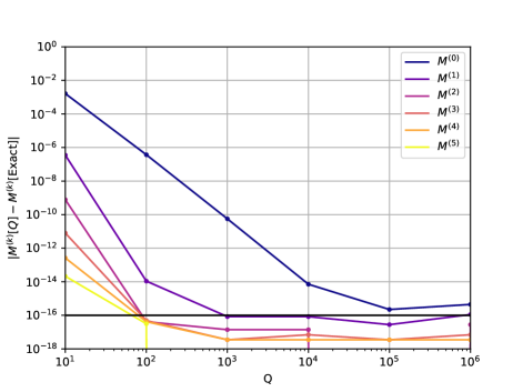
Figure 2: Convergence of the MultiExp moments $M^{(k)}$ with respect to the size of the Gauss-Legendre grid $Q$. The exact moments are $M^{(k)}\equiv\int_{0}^{1}\mathrm{d}x\ \ln^{2}(x)x^{k}=2/(k+1)^{3}$.

IV.2 Convergence of Grids

Figure 3 shows the convergence characteristics of the $N=2$ MultiExp grid vs. the reference grid from the Gill and Chien table. This is representative of grid convergence in the small $N$ limit. Figure 4 shows the same for the $N=45$ grid. The is representative of grid convergence in the medium $N$ limit.

Both figures tell a very similar story. Regular seemingly $\mathcal{O}(Q^{-4})$ convergence occurs for both roots and weights, with the weights having a slightly higher error prefactor. By $Q=10^{5}$ maximum absolute deviations of $<10^{-15}$ in roots and $<10^{-14}$ in weights are achieved for these (and all other correct) grids.

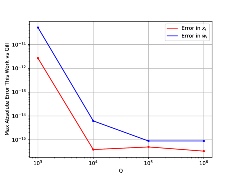
Figure 3: Convergence of the MultiExp grid roots and weights with respect to the size of the Gauss-Legendre grid $Q$, for $N=2$. The reference is the tabulated grid from Gill and Chien. The error characteristic is the maximum absolute deviation.

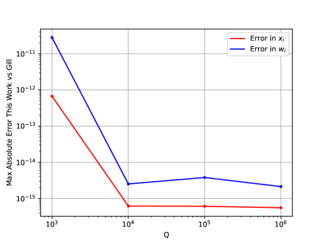
Figure 4: Same as Fig. 3, but for $N=45$.

IV.3 Agreement with Gill’s Grids

Table 1 shows the agreement characteristics with the tabulated Gill and Chien MultiExp grids, for our highest-quality grids obtained with $Q=10^{5}$. We define agreement as the maximum absolute deviation for the roots and weights of each grid, separately. Overall, remarkable agreement is found, with agreement of $\sim 10^{-15}$ in the roots in all cases and $\sim 10^{-14}$ in the weights in most cases.

Table 1: Maximum absolute deviations of MultiExp quadrature grids obtained in this work with $Q=10^{5}$ vs. known MultiExp quadrature grids of Gill and Chien.

$N$	$|\vec{x}-\vec{x}^{\mathrm{Gill}}|_{\infty}$	$|\vec{w}-\vec{w}^{\mathrm{Gill}}|_{\infty}$	Comment
1	2.8E-17	4.4E-16
2	5.0E-16	8.9E-16
3	3.3E-16	1.1E-15
4	3.9E-16	5.6E-16
5	5.6E-16	7.8E-16
6	7.8E-16	2.2E-15
7	5.0E-16	6.7E-16
8	5.6E-16	5.8E-16
9	5.6E-16	2.1E-15
10	4.4E-16	2.2E-15
11	5.6E-16	6.7E-16
12	4.3E-16	2.2E-15
13	5.2E-16	1.7E-15
14	6.7E-16	1.2E-15
15	6.7E-16	1.6E-15
16	7.2E-16	1.0E-15
17	5.6E-16	2.4E-15
18	6.7E-16	3.4E-15
19	6.7E-16	1.8E-15
20	4.7E-16	1.2E-14
21	1.7E-15	2.8E-15
22	4.4E-16	1.1E-15
23	5.6E-16	6.3E-15
24	7.8E-16	4.5E-15
25	4.4E-16	2.8E-15
26	5.6E-16	1.9E-15
30	5.6E-16	3.6E-12	Marginal
35	6.7E-16	3.6E-15
40	5.6E-16	5.9E-15
45	6.1E-16	3.8E-15
50	6.7E-16	3.7E-07	Significant

There are two nontrivial discrepancies between our grids and those of Gill and Chien: $N=30$ (marginal - $4\times 10^{-12}$) and the largest $N=50$ (significant - $4\times 10^{-7}$). Both occur in the weights only and both affect almost all of the weights to the same magnitude (e.g., it is not a single typo in a single weight). We can also rule out accidental issues with the specific value of $Q$ used in our procedure - for these cases, the disagreement is systematic across multiple values of $Q$.

To probe deeper into these discrepancies, we use the Boley-Golub + Golub-Welsch procedure to “boost” the lower MultiExp quadrature rules from the higher ones. As a reminder, the higher MultiExp quadrature rules formally cover the lower ones, so this procedure should be lossless. In Fig. 5, we focus on the mean absolute deviations in the weights arising from this procedure as a metric of accuracy - a similar story occurs in the roots.

After a bit of analysis, the story is fairly simple. Looking at the bottom row: The Gill and Chien $Q=50$ grid is not able to quantitatively reproduce the lower Gill and Chien grids for $N\in\{25,26,30,35,40,45\}$. A similar, smaller but noticeable issue also occurs for $Q=30$. Note that the moderate errors (moderate blue colors) throughout the bottom row are more minor issues that we hypothesize stem from the truncation of the smaller weights to 15 absolute decimal digits in the Gill and Chien tables, which loses a touch of relative precision. Looking at the top row, the grids developed in this work are all quantitatively self consistent, and can quantitatively reproduce all Gill and Chien grids except for the $N=50$ and to a lesser extent the $N=30$ grids that may have problems.

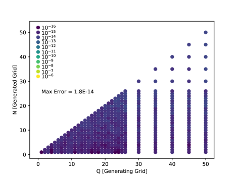
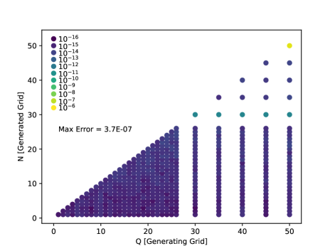
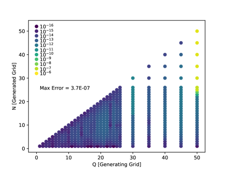
Figure 5: Maximum absolute deviation in weights generated by boosting one MultiExp quadrature rule of size $N$ from another rule of size $Q\geq N$. Top row: quadrature rules generated from this work with $Q=10^{5}$. Bottom row: quadrature rules generated from the tables of Gill and Chien. Left: newly generated quadrature rules compared to this work. Right: newly generated quadrature rules compared to Gill and Chien.

IV.4 Finished MultiExp Quadrature Grids

The highest quality MultiExp quadrature grids computed in this work are obtained for $1\leq N\leq 1000$ using $Q=10^{5}$. Fig. 6 performs a similar analysis as in the previous section, but comparing larger finished MultiExp quadrature grids to smaller ones, up to $N=100$. Overall the story is reassuringly boring: all lower grids are quantitatively reproduced from all higher grids, with very slightly higher errors occurring for weights as compared to roots.

Note that we also computed the grids up to $N=1000$ at $Q=10^{6}$, and find maximum absolute deviation of $6\times 10^{-16}$ in the roots and $3\times 10^{-15}$ in the weights for all 500,500 unique grid points in this set. We also computed the grids up to $N=100$ at $Q=2\times 10^{8}$ with the slower-converging $\gamma=1$, and find vi maximum absolute deviation of $6\times 10^{-16}$ in the roots and $3\times 10^{-15}$ in the weights for all 5,050 unique grid points in this set. All three grids are indistinguishable at very near the double precision machine epsilon, so we have elected to use the $Q=10^{5}$ grid with $\gamma=2$ as our “highest-quality” grid, as it is the smallest grid that we are confident has converged, and is therefore less susceptible to numerical noise in long-running sums and/or underflows in the intermediates.

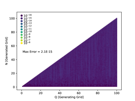
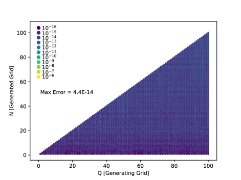
Figure 6: As in Fig. 5 but comparing higher MultiExp grids to all lower MultiExp grids for the highest quality $Q=10^{5}$ grids developed in this work. Comparisons up to $N=100$ are performed. Left panel: maximum absolute deviations in roots. Right panel: maximum absolute deviations in weights.

A visual representation of the finished MultiExp quadrature grids is shown in Figure 1. As with all Gaussian quadratures over smooth measures, the MultiExp quadrature grid exhibits a beautiful root-repulsion property, which manifests as apparent Moiré patterns in the plot.

The Boley-Golub tridiagonal matrix $T_{(N=1000)}$ and all of the associated MultiExp quadrature rules are provided in double precision .npz format for the highest-quality $Q=10^{5}$ grids obtained in this work. These can be obtained at: https://github.com/robparrishqc/multiexp. For the avoidance of all doubt, the complete 16-decimal-digit floating point representation of $T_{(N=100)}$ (which can reproduce all of our grids through Golub-Welsch for up to $N=100$) and the MultiExp quadrature grid for $N=100$ (for reference when others implement their own Golub-Welsch scripts) is provided in Tables 2 and 3 below.

It is extremely difficult to confidently bound all sources of errors that may be occurring in the MultiExp grids obtained below. However, very tight agreement with many of the Gill and Chien grids up to $N=50$, highly regular convergence behavior, a simple and seemingly stable algorithm, and checks of internal Boley-Golub boosting all indicate that extremely accurate grids near the double precision limit have been obtained. Conservatively, we estimate that these grids are good to a maximum absolute deviation of $10^{-14}$ in the roots and $10^{-13}$ in the weights vs. the ground truth. Note that better than one full order of magnitude beyond this estimate was obtained for up to $N=45$ in checks against the sensibly-behaved Gill and Chien grids. Overall, this should be well beyond the accuracy required for density functional theory grid applications. For applications demanding higher accuracy, testing against a massive systemic quadrature like Gauss-Laguerre or remapped Gauss-Legendre should be performed.

IV.5 Integration Filter Functions

To close this section, we will take a moment to explore an experimental topic: integration “filter functions.” Let us consider the integration of an arbitrary normalized Slater function with exponent $\alpha$,

$$I(\alpha)\equiv\int_{0}^{\infty}\mathrm{d}r\ r^{2}N\exp(-\alpha r)=1$$

$$\approx\sum_{i=1}^{N}w_{i}N\exp(-\alpha r_{i}):\ N\equiv\left(\frac{2}{\alpha^{3}}\right)^{-1}$$ (21)

We can define the Slater filter function as the integration error $\Delta^{\mathrm{Slater}}(\alpha)\equiv I(\alpha)-1$. Here and throughout this section we consider the nondimensional case $R=1$.

Figure 7 shows the Slater filter function for several representative $N$ using the MultiExp grids built in this work and also those of Gill and Chien where the latter are available. Looking at the figure deeply, we realize that there seems to be a bit of serendipity going on here with these MultiExp quadrature grids. We are guaranteed by construction that this quadrature rule exactly integrates $\alpha=k\ \forall\ k\in{1,\ldots,2N}$. This is apparent from the zero crossing at $\alpha=1$ and the integrally spaced zeros crossings for higher $\alpha$. However, up to this point, we have had no guarantee or even conception of the performance for $\alpha$ points between the integral lattice. However, the MultiExp appears to be doing considerably more than just providing exact collocation at the integral lattice - in fact, it seems to be exponentially suppressing the errors for intermediate $\alpha$, leading to a large flat spot in the middle of the plot that coalesces with errors down near the machine epsilon for a significant range of $\alpha$. Also note that this error-suppresed region appears to promulgate to much higher $\alpha$ than strictly conctracted by the integral lattice (highest lattice points at $\alpha=2N$ indicated in the darker vertical lines).

As one minor note, most of the larger Gill and Chien quadratures exhibit the slightly worse coalesced errors in the “first” region of disagreement on the left side of the coalesced region - we attribute this to truncation errors in the weights as reported to 15 absolute decimal digits, and find that this does not significantly affect the filter functions for smoother integrands such as Gaussians (see next paragraph). However, the “second” region of disagreement on the right side of the coalesced region for $N=50$ is much more apparent and is unique to the $N=50$ rule - we attribute this to the previously-mentioned problem with this tabulated grid. Of particular note, this discrepancy poisons the quality of the Slater integration filter in the region from $\alpha\sim 10^{+2}-10^{+3}$, which might have significant practical ramifications. It might well be the case that this grid is much more accurate than previously advertised.

Another interesting case is when we consider instead a normalized Gaussian integrand with arbitrary exponent $\beta$,

$$J(\beta)\equiv\int_{0}^{\infty}\mathrm{d}r\ r^{2}N\exp(-\beta r^{2})=1$$

$$\approx\sum_{i=1}^{N}w_{i}N\exp(-\alpha r_{i}^{2}):\ N\equiv 4\pi\left(\frac{\pi}{\beta}\right)^{-3/2}$$ (22)

As above, we will define the Gaussian filter function as the integration error $\Delta^{\mathrm{Gaussian}}(\beta)\equiv J(\beta)-1$.

Figure 8 shows the Gaussian filter function for several representative $N$ using the MultiExp grids built in this work and also those of Gill and Chien where the latter are available. For this case, we no longer have any concrete idea of where exact integration is guaranteed (e.g., the zeros are now $N$-dependent). However, a similar behavior of coalescence near the machine precision is observed for a large range of $\beta$, with the size of this region increasing with $N$. As promised in the last paragraph, the minor coalescence issue with the $N=25$ Gill grid is not an issue for smoother functions like Gaussians, as the two red curves are qualitatively indistinguishable. However, the $N=50$ grids have significant discrepancies which poison the region of coalescence and creep up above $10^{-6}$ integration error. Overall, the broad accuracy of the MultiExp grids is amazing - for $N=100$, Gaussian exponents from $10^{0}$ to $10^{+4}$ are essentially exactly integrated in double precision, while Gaussian exponents from $10^{-1}$ to $10^{+5}$ are integrated to $10^{-8}$ relative precision.

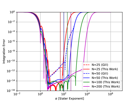
Figure 7: Slater integration filter function for various MultiExp quadratures. The plot shows the error encountered when integrating a normalized Slater function with exponent $\alpha$, while using the dimensionless choice of $R=1$. The vertical lines indicate the maximum guaranteed exactly-integrated Slater exponent of $\alpha=2N$.

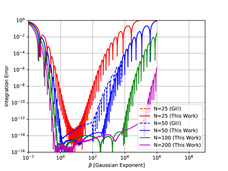
Figure 8: Gaussian integration filter function for various MultiExp quadratures. The plot shows the error encountered when integrating a normalized Gaussian function with exponent $\beta$, while using the dimensionless choice of $R=1$.

V Summary and Outlook

Overall, this story is fairly simple. We have produced the MultiExp quadrature table for all $N\leq 1000$ to what we posit is better than 14(13) decimal digits of the maximum absolute deviations of the roots(weights). This was done by merging the recently-developed extremely high-order Gauss-Legendre quadrature methods of Bogaert with the Boley-Golub and Golub-Welsch algorithms.

The combination of a high-order known quadrature rule with Boley-Golub + Golub-Welsch in a difficult weight function may have further runway in electronic structure and beyond. I have often used Boley-Golub in the past for things like Rys and Boys tables, but usually with better-behaved weight functions that only required $Q=200$ or so. MultiExp’s weight function strikes me as unusually difficult.

As for the MultiExp grids, it may be that they deserve greater study for medium- and high-quality density functional theory grids. The integration filter function analysis shows compelling performance for multiscale Slater and Guassian functions which is serendipitously beyond what is expected from even Gaussian quadrature theory. The broad regions of coalesced double precision accuracy point to a loose idea that a combination of careful selection of atomic partition function (acting as a sort of dealiasing filter) together with well-chosen Lebedev and MultiExp spherical grids (acting as a sort of an analog-to-digital coverter) might be able to produce extremely accurate integration over density-involving integrands.

It is my hope to make the simple web respository of tabulated MultExp grids provided at https://github.com/robparrishqc/multiexp dynamic - I will try post updates on accuracy improvements, accuracy bounds, or rules for larger $N$ as they are obtained.

Acknowledgements: Sincere thanks to I. Bogaert for writing such a clear and marvelous paper on large-scale Gauss-Legendre quadratures.

Disclaimer: RMP owns stock/options in QC Ware Corp.

Table 2: Table of $N=100$ MultiExp quadrature developed with the highest-quality $Q=10^{5}$ used in this work. Table contains both the quadrature rule, and the diagonal / superdiagonal of the associated tridiagonal Boley-Golub matrix. The latter can be used with the Golub-Welsch to obtain all lower quadrature rules. Zero-based ordering is used within the table. Part 1 of 2.

$k$	$x_{k}$	$w_{k}$	$T_{k+1,k+1}$	$T_{k,k+1}$
0	1.0085604224960984E-04	2.4870306762083891E-02	1.2500000000000003E-01	1.4142135623730949E+00
1	6.2370830580574081E-04	4.1069176975224012E-02	3.8851351351351354E-01	1.4632852434517696E-01
2	1.6111135319247123E-03	5.0506092347931963E-02	4.4960948964368064E-01	2.1415281692418647E-01
3	3.0668769586458212E-03	5.6613009441253949E-02	4.7132321389185050E-01	2.3175854175497282E-01
4	4.9920519775517218E-03	6.0669039914305153E-02	4.8148774770913866E-01	2.3895834934512467E-01
5	7.3864040114336353E-03	6.3322642015236907E-02	4.8705873760139035E-01	2.4260216275101654E-01
6	1.0248816678655993E-02	6.4957405384297978E-02	4.9044203361145278E-01	2.4469971118791925E-01
7	1.3577463486490179E-02	6.5822739841657679E-02	4.9265083085488964E-01	2.4601697895485777E-01
8	1.7369896640950108E-02	6.6091611891759217E-02	4.9417258087122390E-01	2.4689804818183456E-01
9	2.1623099391943873E-02	6.5889742995765208E-02	4.9526558057420966E-01	2.4751623882089294E-01
10	2.6333520074391794E-02	6.5311842329492720E-02	4.9607714413613979E-01	2.4796659902484317E-01
11	3.1497096119372507E-02	6.4431290584450074E-02	4.9669630457035846E-01	2.4830479793311860E-01
12	3.7109272227740756E-02	6.3306241999689830E-02	4.9717945800257973E-01	2.4856520018151709E-01
13	4.3165015005529855E-02	6.1983641827715076E-02	4.9756374195292374E-01	2.4876995136133967E-01
14	4.9658825402078673E-02	6.0501968356295642E-02	4.9787442418046540E-01	2.4893384402785859E-01
15	5.6584749772155420E-02	5.8893161721076080E-02	4.9812918259335398E-01	2.4906706412523832E-01
16	6.3936390085429201E-02	5.7184015991635750E-02	4.9834068656355734E-01	2.4917681101791719E-01
17	7.1706913627772081E-02	5.5397206433533040E-02	4.9851820881381631E-01	2.4926828978783769E-01
18	7.9889062427192889E-02	5.3552062420907348E-02	4.9866866281552119E-01	2.4934533915605897E-01
19	8.8475162565092622E-02	5.1665159057777903E-02	4.9879728838755616E-01	2.4941084029640354E-01
20	9.7457133485575775E-02	4.9750777045557783E-02	4.9890811555506359E-01	2.4946698975587775E-01
21	1.0682649738281912E-01	4.7821265134587045E-02	4.9900428501941568E-01	2.4951548575808452E-01
22	1.1657438872363589E-01	4.5887329432307521E-02	4.9908827375964365E-01	2.4955765793855311E-01
23	1.2669156394605771E-01	4.3958267028700149E-02	4.9916205656282697E-01	2.4959455932233066E-01
24	1.3716841136288330E-01	4.2042156698880902E-02	4.9922722347088877E-01	2.4962703259914357E-01
25	1.4799496129035877E-01	4.0146016141017954E-02	4.9928506637923215E-01	2.4965575858804051E-01
26	1.5916089641552880E-01	3.8275932851582095E-02	4.9933664371345632E-01	2.4968129215845308E-01
27	1.7065556241073593E-01	3.6437174033842598E-02	4.9938282930579375E-01	2.4970408918506648E-01
28	1.8246797879981239E-01	3.4634279683658842E-02	4.9942434973444111E-01	2.4972452700576633E-01
29	1.9458685007741233E-01	3.2871142066682860E-02	4.9946181313698762E-01	2.4974292011245156E-01
30	2.0700057708045777E-01	3.1151074102617683E-02	4.9949573165283506E-01	2.4975953230313847E-01
31	2.1969726860867511E-01	2.9476868641935158E-02	4.9952653905546629E-01	2.4977458617882725E-01
32	2.3266475328956535E-01	2.7850850214113904E-02	4.9955460471797192E-01	2.4978827062800227E-01
33	2.4589059168178964E-01	2.6274920512261948E-02	4.9958024475825580E-01	2.4980074677170286E-01
34	2.5936208860982973E-01	2.4750598633950422E-02	4.9960373099668115E-01	2.4981215272064283E-01
35	2.7306630572181650E-01	2.3279056905569379E-02	4.9962529820354401E-01	2.4982260740809673E-01
36	2.8699007426160728E-01	2.1861152965099964E-02	4.9964514999965765E-01	2.4983221369819270E-01
37	3.0112000804549349E-01	2.0497458656735038E-02	4.9966346368876136E-01	2.4984106092202224E-01
38	3.1544251663330630E-01	1.9188286193387662E-02	4.9968039423719862E-01	2.4984922695883946E-01
39	3.2994381868316508E-01	1.7933711964510341E-02	4.9969607756862916E-01	2.4985677995326103E-01
40	3.4460995547864703E-01	1.6733598302894743E-02	4.9971063330530058E-01	2.4986377973943913E-01
41	3.5942680461674748E-01	1.5587613472126192E-02	4.9972416705964079E-01	2.4987027902798681E-01
42	3.7438009384464777E-01	1.4495250093739014E-02	4.9973677235856101E-01	2.4987632439976462E-01
43	3.8945541503298392E-01	1.3455842198038762E-02	4.9974853226624999E-01	2.4988195714162623E-01
44	4.0463823827303552E-01	1.2468581053568668E-02	4.9975952075826957E-01	2.4988721395220503E-01
45	4.1991392608500494E-01	1.1532529906098689E-02	4.9976980388958997E-01	2.4989212754032905E-01
46	4.3526774772434540E-01	1.0646637737994935E-02	4.9977944079113540E-01	2.4989672713433625E-01
47	4.5068489357290376E-01	9.8097521420505551E-03	4.9978848452303570E-01	2.4990103891712992E-01
48	4.6615048960148436E-01	9.0206313898332259E-03	4.9979698280765433E-01	2.4990508639909725E-01
49	4.8164961189030181E-01	8.2779557627929018E-03	4.9980497866137641E-01	2.4990889073882697E-01

Table 3: As in Tab. 2. Part 2 of 2.

$k$	$x_{k}$	$w_{k}$	$T_{k+1,k+1}$	$T_{k,k+1}$
50	4.9716730119366948E-01	7.5803382044358865E-03	4.9981251094082646E-01	2.4991247101981312E-01
51	5.1268857753518005E-01	6.9263343434874313E-03	4.9981961481651499E-01	2.4991584448991430E-01
52	5.2819845481955596E-01	6.3144519308655101E-03	4.9982632218472550E-01	2.4991902676918848E-01
53	5.4368195544728815E-01	5.7431597272897842E-03	4.9983266202668369E-01	2.4992203203078781E-01
54	5.5912412491814933E-01	5.2108958732641373E-03	4.9983866072257294E-01	2.4992487315883147E-01
55	5.7451004640964154E-01	4.7160757688626577E-03	4.9984434232678232E-01	2.4992756188654330E-01
56	5.8982485531643769E-01	4.2570994870939436E-03	4.9984972880975165E-01	2.4993010891742623E-01
57	6.0505375373688686E-01	3.8323587415317051E-03	4.9985484027097654E-01	2.4993252403181032E-01
58	6.2018202489268826E-01	3.4402434262823332E-03	4.9985969512703088E-01	2.4993481618075994E-01
59	6.3519504746787792E-01	3.0791477441502479E-03	4.9986431027790873E-01	2.4993699356902291E-01
60	6.5007830985333659E-01	2.7474759370127787E-03	4.9986870125448857E-01	2.4993906372846089E-01
61	6.6481742428310520E-01	2.4436476308510751E-03	4.9987288234953681E-01	2.4994103358318787E-01
62	6.7939814084888117E-01	2.1661028065921165E-03	4.9987686673431220E-01	2.4994290950746986E-01
63	6.9380636137917984E-01	1.9133064068387808E-03	4.9988066656255520E-01	2.4994469737729122E-01
64	7.0802815316976475E-01	1.6837525876843753E-03	4.9988429306339882E-01	2.4994640261636614E-01
65	7.2204976255208009E-01	1.4759686240913507E-03	4.9988775662452656E-01	2.4994803023727005E-01
66	7.3585762828657719E-01	1.2885184767437005E-03	4.9989106686673296E-01	2.4994958487827185E-01
67	7.4943839476798102E-01	1.1200060278347796E-03	4.9989423271089062E-01	2.4995107083637444E-01
68	7.6277892502972255E-01	9.6907799291465755E-04	4.9989726243818494E-01	2.4995249209700282E-01
69	7.7586631353495361E-01	8.3442651567650831E-04	4.9990016374439278E-01	2.4995385236072101E-01
70	7.8868789874175871E-01	7.1479145239608001E-04	4.9990294378885741E-01	2.4995515506731661E-01
71	8.0123127543040029E-01	6.0896235264631710E-04	4.9990560923875160E-01	2.4995640341754122E-01
72	8.1348430678065564E-01	5.1578014287398909E-04	4.9990816630913348E-01	2.4995760039276643E-01
73	8.2543513618755138E-01	4.3413851944353770E-04	4.9991062079925319E-01	2.4995874877277999E-01
74	8.3707219880405026E-01	3.6298505781634868E-04	4.9991297812550012E-01	2.4995985115192002E-01
75	8.4838423279951236E-01	3.0132204463237578E-04	4.9991524335134291E-01	2.4996090995372314E-01
76	8.5936029032304118E-01	2.4820703959349040E-04	4.9991742121457577E-01	2.4996192744423995E-01
77	8.6998974816110197E-01	2.0275317420627710E-04	4.9991951615213975E-01	2.4996290574415617E-01
78	8.8026231807912902E-01	1.6412919462128724E-04	4.9992153232276326E-01	2.4996384683983816E-01
79	8.9016805683714861E-01	1.3155925600465745E-04	4.9992347362764172E-01	2.4996475259341247E-01
80	8.9969737586980014E-01	1.0432247608897793E-04	4.9992534372934228E-01	2.4996562475197356E-01
81	9.0884105062150600E-01	8.1752255773420523E-05	4.9992714606911348E-01	2.4996646495600530E-01
82	9.1759022952794977E-01	6.3235374872911318E-05	4.9992888388274231E-01	2.4996727474709216E-01
83	9.2593644263548436E-01	4.8210871351274372E-05	4.9993056021510573E-01	2.4996805557498722E-01
84	9.3387160985062678E-01	3.6168712611043006E-05	4.9993217793352990E-01	2.4996880880409839E-01
85	9.4138804881247373E-01	2.6648267649900886E-05	4.9993373974007382E-01	2.4996953571944552E-01
86	9.4847848238176335E-01	1.9236589130072258E-05	4.9993524818283103E-01	2.4997023753213915E-01
87	9.5513604574162481E-01	1.3566514639098464E-05	4.9993670566634185E-01	2.4997091538442229E-01
88	9.6135429310711895E-01	9.3145966474992437E-06	4.9993811446118974E-01	2.4997157035431636E-01
89	9.6712720404426178E-01	6.1988708890889789E-06	4.9993947671286099E-01	2.4997220345990456E-01
90	9.7244918940592040E-01	3.9764731017865003E-06	4.9994079444992690E-01	2.4997281566328680E-01
91	9.7731509690548601E-01	2.4411142694155630E-06	4.9994206959160592E-01	2.4997340787423311E-01
92	9.8172021637864459E-01	1.4204246971928530E-06	4.9994330395476461E-01	2.4997398095356077E-01
93	9.8566028485295398E-01	7.7317743420403144E-07	4.9994449926039919E-01	2.4997453571626216E-01
94	9.8913149172461112E-01	3.8640172437758307E-07	4.9994565713964489E-01	2.4997507293439988E-01
95	9.9213048486257771E-01	1.7239732240031524E-07	4.9994677913934638E-01	2.4997559333979216E-01
96	9.9465438020399766E-01	6.5660651994930723E-08	4.9994786672723462E-01	2.4997609762650316E-01
97	9.9670078450658928E-01	1.9733910354580023E-08	4.9994892129673407E-01	2.4997658645315632E-01
98	9.9826787957629104E-01	3.9883338154167677E-09	4.9994994417142968E-01	2.4997706044508378E-01
99	9.9935496638135868E-01	3.5293623678895923E-10	4.9995093660922957E-01	2.4997752019632452E-01

References

- Becke (1988) A. D. Becke, The Journal of chemical physics 88, 2547 (1988).
- Stratmann et al. (1996) R. E. Stratmann, G. E. Scuseria, and M. J. Frisch, Chemical physics letters 257, 213 (1996).
- Lebedev (1976) V. I. Lebedev, USSR Computational Mathematics and Mathematical Physics 16, 10 (1976).
- Lebedev and Laikov (1999) V. I. Lebedev and D. Laikov, in Doklady Mathematics, Vol. 59 (1999) pp. 477–481.
- Murray et al. (1993) C. W. Murray, N. C. Handy, and G. J. Laming, Molecular Physics 78, 997 (1993).
- Treutler and Ahlrichs (1995) O. Treutler and R. Ahlrichs, The Journal of Chemical Physics 102, 346 (1995).
- Mura and Knowles (1996) M. E. Mura and P. J. Knowles, The Journal of chemical physics 104, 9848 (1996).
- Mitani and Yoshioka (2012) M. Mitani and Y. Yoshioka, Theoretical Chemistry Accounts 131, 1 (2012).
- Shizgal et al. (2017) B. D. Shizgal, N. Ho, and X. Yang, Journal of Mathematical Chemistry 55, 413 (2017).
- Gill and Chien (2003) P. M. Gill and S.-H. Chien, Journal of computational chemistry 24, 732 (2003).
- Chien and Gill (2006) S.-H. Chien and P. M. Gill, Journal of computational chemistry 27, 730 (2006).
- (12) P. M. Gill and S.-H. Chien, Roots and weights for multiexp quadrature, https://rsc.anu.edu.au/pgill/multiexp.php, retrieved 27 Mar 2023.
- Boley and Golub (1987) D. Boley and G. H. Golub, Inverse problems 3, 595 (1987).
- Fernandes and Atchley (2006) A. D. Fernandes and W. R. Atchley, Evolutionary Bioinformatics 2, 117693430600200010 (2006).
- Golub and Welsch (1969) G. H. Golub and J. H. Welsch, Mathematics of computation 23, 221 (1969).
- Kahan (1965) W. Kahan, Communications of the ACM 8, 40 (1965).
- Klein (2006) A. Klein, Computing 76, 279 (2006).
- Bogaert (2014) I. Bogaert, SIAM Journal on Scientific Computing 36, A1008 (2014).
- Townsend (2015) A. Townsend, SIAM News 48, 1 (2015).