Cosmic acceleration in entropic cosmology.

Abstract

In this paper we study the viability of an entropic cosmological model. The effects of entropic gravity are derived from a modified entropy-area relationship with a volumetric entropy term. This model describes a late time limit cosmic acceleration, whose origin is related to a volumetric term in the entropy. Moreover, we analyze the phenomenological implications of the entropic model using the Supernovae Pantheon compilation and the observational Hubble parameter data to find consistency with cosmological observations. Finally, we show the equivalence between the entropic model and a brane world cosmological model, by means of an effective geometrical construction.

1 Introduction

The verification of the current acceleration of the Universe opened a new avenue of research in cosmology. The best model is the standard model of cosmology, known as lambda cold dark matter ($\Lambda CDM$). This model is based on the existence of matter that has anomalous physical properties. In particular, it conjectures the existence of a cosmological constant $\Lambda$ as the origin of the source of the late time acceleration. Although there is good phenomenological agreement with observations, there are serious theoretical concerns that need to be understood [1, 2].

A different approach is to assume that this acceleration is a consequence of a modified theory of gravity and several ideas have been pursued [3, 4, 5, 6]. One possibility, is to consider gravity as an emergent phenomenon [7]. The renewed interest in this idea started with Verlinde [8], where the author claims that Newtonian gravity is an emergent force. Moreover, modifications to gravity are induced by changing the entropy-area relation. In this context, the possibility of a common origin of dark matter and dark energy has been proposed [9]. The dark matter predictions for this theory have been put to test in several works [10, 11, 12]. Following this line of reasoning, a connection with dark energy was explored. More precisely, an entropic origin to the cosmological constant was proposed. This is achieved by considering a cosmological model that is derived from the Clausius relation and a modified entropy-area relationship. The modified Friedmann equations in the limit $t\to\infty$ and $\rho\to 0$, give a de Sitter Universe. This allowed to define an effective cosmological constant [13] and is related to the modification to Hawking-Bekenstein entropy. Considering the effective cosmological constant at $t\to\infty$, it points that at present times this model describes an accelerating universe, and hence it should be equivalent to a cosmological model with a dark energy component. The purpose of this paper is to study the phenomenology of this model by adjusting the parameters using cosmological data. Furthermore, by comparing it with the $\Lambda CDM$ model, we find time varying dark energy component that causes the cosmic acceleration and find the effective dark energy parameter $\omega_{eff}$ for the barotropic equation of state. Finally, as an important feature, we will discuss the equivalence of the entropic cosmological model with the Dvali-Gabadadze-Porrati (DGP) model, which emerges in the brane worlds framework. Exploiting this equivalence, we can relate the free parameter of our model with the characteristic distance scale of the DGP cosmology.

This paper is arranged as follows. In section 2 we review the derivation of the modified Friedmann equations as well as some theoretical implications, mainly the de Sitter late time behavior and therefore the effective cosmological constant. In section 3, we show that the model satisfies the cosmological tests and is therefore viable. Finally, section 4 is devoted to concluding remarks.

2 The modified Friedmann equation from the new entropy-area relationship

Let us start by reviewing the derivation of the modified Friedmann equations based on the application of the Clausius relation on the apparent horizon of the FRW universe.

First, we consider a FRW universe described by the metric

$$ds^{2}=-dt^{2}+a^{2}(t)\left(\frac{dr^{2}}{1-\kappa r^{2}}+r^{2}d{\Omega}^{2}\right).$$ (2.1)

The apparent horizon of the FRW universe is defined through the condition $h^{ab}\partial_{a}\tilde{r}\partial_{b}\tilde{r}=0$, where $\tilde{r}=a(t)r$ and $h^{ab}$ is identified by writing the metric as $ds^{2}=h_{ab}dx^{a}dx^{b}+\tilde{r}^{2}d\Omega^{2}$. This condition leads us to the radius of the apparent horizon

$$\tilde{r}^{2}_{A}=\left(H^{2}+\kappa/a^{2}\right)^{-1}.$$ (2.2)

To apply the Clausius relation we use the temperature and entropy on the apparent horizon. For this work, we assume that the temperature is $T=1/2\pi\tilde{r}_{A}$ and the entropy is given by

$$S(A)=\frac{A}{4G}+\epsilon\left(\frac{A}{4G}\right)^{3/2},$$ (2.3)

where $A$ is the area of the apparent horizon and $\epsilon$ is a free parameter of the model. The modified entropy-area relationship is motivated by a previous work [13], where it is inferred that the inclusion of a volumetric term is related to the late time acceleration of the Universe.

Using the energy-momentum tensor for a perfect fluid of energy density $\rho$ and pressure $P$, the Clausius relation on the apparent horizon of the FRW universe gives

$$4\pi\tilde{r}_{A}^{2}(\rho+P)H\tilde{r}_{A}dt=\frac{1}{8\pi G}\frac{1}{\tilde{r}_{A}}\left[1+\frac{3\epsilon}{\sqrt{2G}}A^{1/2}\right]dA.$$ (2.4)

From the time derivative of $A$ and the standard continuity equation $\dot{\rho}+3H(p+\rho)=0$, we arrive to the modified Friedmann equations

$$\frac{8\pi G}{3}\rho=\left(H^{2}+\frac{\kappa}{a^{2}}\right)+\sqrt{\frac{{9\pi}}{G}}\epsilon\left(H^{2}+\frac{\kappa}{a^{2}}\right)^{1/2}.$$ (2.5)

The solution to Eq.(2.5) for a barotropic equation of state of the perfect fluid $P=\omega\rho$, with $\kappa=0$ is given by

$$144\sqrt{\pi}G\rho_{0}(\omega+1)t=3a\sqrt{96G\rho_{0}a^{3\omega+1}+\frac{81\epsilon^{2}a^{6\omega+4}}{G}}-\frac{27\epsilon a^{3(\omega+1)}}{\sqrt{G}}$$

$$+ \frac{32G^{3/2}\rho_{0}a^{-3(1+\omega)/2}\sqrt{32G^{2}\rho_{0}a^{3\omega+1}+27\epsilon^{2}a^{6\omega+4}}\sinh^{-1}\left(\frac{3\sqrt{\frac{3}{2}}\epsilon a^{3(1+\omega)/2)}}{4G\sqrt{\rho_{0}}}\right)}{\epsilon\sqrt{27\epsilon^{2}a^{3\omega+3}+32G^{2}\rho_{0}}}.$$

In the early-time limit, the behaviour of the scale factor is the same as the one derived from the usual Friedmann equation for a perfect fluid with a barotropic equation of state. However, the most important feature of this model is that in the late time limit, the scale factor exhibits an exponential growth modulated by the effective cosmological constant

$$\Lambda_{eff}=\frac{27\pi}{G}\epsilon^{2}.$$ (2.7)

Interestingly, this late-time exponential behaviour is provided by the volumetric correction term in Eq.(2.3). Finally, it is important to emphasize that our model does not have a priori a cosmological constant, or a dark energy component of any kind.

3 Phenomenological Tests

From the discussion in the previous section, we consider the cosmic acceleration of the model and contemplate an entropic origin for the dark energy component. In particular, the dark energy component is a consequence of the volumetric part of the entropy-area relationship.

In order to proceed with the phenomenological analysis of our model, it is suitable to express the modified Friedmann equations in terms of density parameters. First, let us note that Eq.(2.5) can be expressed as

$$H^{2}+\frac{\kappa}{a^{2}}=\frac{8\pi G}{3}\rho+\frac{1}{2}\frac{9\pi}{G}\epsilon^{2}+\sqrt{\frac{1}{4}\left(\frac{9\pi}{G}\epsilon^{2}\right)^{2}+\left(\frac{9\pi}{G}\epsilon^{2}\right)\left(\frac{8\pi G}{3}\rho\right)},$$ (3.1)

this equation encourages us to define the parameter associated to $\epsilon$ as

$$\Omega_{\epsilon 0}\equiv\frac{1}{2H_{0}^{2}}\frac{{9\pi}}{G}\epsilon^{2},$$ (3.2)

as usual, the parameters associated to matter and spatial curvature are defined as

$$\Omega_{M0}=\frac{8\pi G}{3H_{0}^{2}}\rho_{0},\quad\Omega_{\kappa 0}=-\frac{\kappa}{a_{0}^{2}H_{0}^{2}}.$$ (3.3)

After considering non-relativistic matter for which $\rho=\rho_{0}(1+z)^{3}$ where $z$ is the redshift $1+z=1/a$, equation Eq.(3.1) can be written in terms of the above parameters as

$$H^{2}(z)=H_{0}^{2}\left[\Omega_{M0}(1+z)^{3}+\Omega_{\kappa 0}(1+z)^{2}+\Omega_{\epsilon 0}+\sqrt{\Omega_{\epsilon 0}^{2}+2\Omega_{\epsilon 0}\Omega_{M0}(1+z)^{3}}\right],$$ (3.4)

we can compare this equation with the usual Friedmann equation

$$H^{2}(z)=H_{0}^{2}\left\{\Omega_{\kappa 0}(1+z)^{2}+\Omega_{M0}(1+z)^{3}+\Omega_{X0}(1+z)^{3\left(1+\omega_{X}\right)}\right\},$$ (3.5)

where $\Omega_{X0}$ represents a dark energy component with an equation of state parameters given by $\omega_{X}$. The usual cosmological constant is mimicked by $\omega_{X}=-1,$ in this case $\Omega_{X0}=\Omega_{\Lambda}$. For redshift $z=0$, the modified Friedmann equations yield

$$\Omega_{M0}+\Omega_{\kappa 0}+\Omega_{\epsilon 0}+\sqrt{\Omega_{\epsilon 0}^{2}+2\Omega_{\epsilon 0}\Omega_{M0}}=1,$$ (3.6)

which is to be recognized as our modified Friedmann constriction for the density parameters. This constriction clearly differs from the usual constriction $\sum_{i}\Omega_{i0}=1$, obtained from Eq.(3.5). We can further rewrite equation Eq.(3.4) in a simpler form by noting that

$$\Omega_{M0}(1+z)^{3}+\Omega_{\epsilon 0}+\sqrt{\Omega_{\epsilon 0}^{2}+2\Omega_{\epsilon 0}\Omega_{M0}(1+z)^{3}}=\frac{1}{2}\left[\sqrt{\Omega_{\epsilon 0}}+\sqrt{\Omega_{\epsilon 0}+2\Omega_{M0}(1+z)^{3}}\right]^{2},$$ (3.7)

therefore we have

$$H^{2}(z)=H_{0}^{2}\left\{\Omega_{\kappa 0}(1+z)^{2}+\frac{1}{2}\left[\sqrt{\Omega_{\epsilon 0}}+\sqrt{\Omega_{\epsilon 0}+2\Omega_{M0}(1+z)^{3}}\right]^{2}\right\},$$ (3.8)

and the modified Friedmann constriction Eq.(3.6) becomes

$$\Omega_{\kappa 0}+\frac{1}{2}\left(\sqrt{\Omega_{\epsilon 0}}+\sqrt{\Omega_{\epsilon 0}+2\Omega_{M0}}\right)^{2}=1.$$ (3.9)

With the results obtained so far, we can perform some basic observational tests in order to roughly estimate a range where the parameters of the model are compatible with background cosmology. To do so, let us fit the parameters of our model by comparing it with two sets of observational data and minimizing the $\chi^{2}$ estimator of goodness of fit,

$$\chi_{O}^{2}=\sum_{i=1}^{N}\left(\frac{O_{th}(z_{i},\Theta)-O_{obs}(z_{i})}{\sigma_{obs}^{i}}\right)^{2},$$ (3.10)

where $O$ is the physical quantity under consideration, with theoretical predictions $O_{th}$ depending on certain parameters $\Theta$, and reported observational values $O_{obs}$ with corresponding uncertainties $\sigma_{obs}$, and $N$ is the number of data points. The data sets that we use are the following.

• Supernovae 1a. (SN Ia) Standard candles, such as type 1a supernovae, are particularly useful for fixing the background cosmology in theories of modified gravity. We use the Pantheon compilation [16], which consists of 1048 supernovae in the range $0.01<z<2.3$. The data reported in [16] consists of apparent magnitudes $m_{b}$, which are related to luminosity distance in megaparsecs by

  $$m_{b}-M=5\log_{10}\left(d_{L}/{\rm Mpc}\right)+25,$$ (3.11)

  where $M$ is the absolute B-band magnitude of a fiducial SN Ia. Using this relation, assuming a spatially flat universe, and using Eq.(3.8), Eq.(3.9) and the luminosity distance

  $$d_{L}=(1+z)H_{0}\int_{0}^{z}\frac{dz^{\prime}}{H(z^{\prime})},$$ (3.12)

  we construct the theoretical predictions for $m_{b}$, depending on the parameter $\Omega_{M0}$, and we minimize Eq.(3.10) for $O=m_{b}$ and $N=1048$. The parameter $H_{0}$ is not included in the minimization of $\chi^{2}$, instead, it is determined as $H_{0}=71.4$ in the region $z<0.05$ using the linear Hubble relation.

• Hubble parameter data. (OHD) We use the compilation provided by [17], which consists of 36 data points for $H(z)$, determined using cosmic chronometers and baryon acoustic oscillations, in the range $z<2.36$ [18, 19, 20, 21, 22, 23, 24, 25, 26, 27]. We compare this data to the predictions of Eq.(3.8) together with Eq.(3.9) and $\Omega_{\kappa 0}=0$, obtaining the parameters $(H_{0},\Omega_{M0})$ that minimize the $\chi^{2}$ estimator, Eq.(3.10), with $O=H$ and $N=36$.

The best fit parameters for each of the data sets described above are reported in Table 1, together with their reduced $\chi^{2}$.

	$H_{0}$	$\Omega_{M0}$	$\chi_{red}^{2}$
SN Ia	71.4	$0.194$	$0.93$
OHD	$66.7$	$0.234$	$0.48$

Table 1: Best fit values and $\chi^{2}$ tests for the model described by Eq.(3.8) with $\Omega_{\kappa}0=0$, contrasted against supernovae 1a and Hubble parameter data. The small value of $\chi^{2}$ for OHD is a consequence of the large uncertainties in these measurements.

In Fig. (1) we show the luminosity distance of SN Ia in the Pantheon compilation (left panel) and the evolution of the Hubble parameter (right panel). In each plot, we include as a reference the predictions of $\Lambda$CDM, and the predictions of our model for two sets of parameters: one corresponds to the best fit to $m_{b}$ described in the first item above (dashed lines), and the other is the best fit to $H(z)$ described in the second item (solid lines). Although the determined parameter was $\Omega_{M0}$, the value for the parameter $\Omega_{\epsilon 0}$ can be obtained from the constriction Eq.(3.9), i.e. we obtain two sets of values $(\Omega_{M0},\Omega_{\epsilon 0})$ which we will use in all the subsequent analysis.

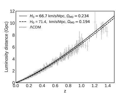
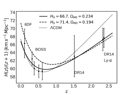
Figure 1: Luminosity distance for SN Ia in the Pantheon compilation (left) and some sample points of $H(z)$ in the compilation [17] (right). The curves in each plot correspond to the predictions of $\Lambda$CDM (dotted), the entropic model Eq.(3.8) fitted to SN Ia (dashed) and the entropic model fitted to evolution of $H(z)$ (solid).

The $z-$dependent density parameters $\Omega_{M}$ and $\Omega_{\epsilon}$ can be obtained in a straightforward manner, resulting in

$$\Omega_{M}(z)=\frac{\Omega_{M0}(1+z)^{3}}{\Omega_{\kappa 0}(1+z)^{2}+\frac{1}{2}\left[\sqrt{\Omega_{\epsilon 0}}+\sqrt{\Omega_{\epsilon 0}+2\Omega_{M0}(1+z)^{3}}\right]^{2}},$$ (3.13)

and

$$\Omega_{\epsilon}(z)=\frac{\Omega_{\epsilon 0}}{\Omega_{\kappa 0}(1+z)^{2}+\frac{1}{2}\left[\sqrt{\Omega_{\epsilon 0}}+\sqrt{\Omega_{\epsilon 0}+2\Omega_{M0}(1+z)^{3}}\right]^{2}}.$$ (3.14)

In Fig.(2) we show the comparison between the behaviour of the density parameters of our model Eq.(3.13) and Eq.(3.14) and the behaviour of the density parameters of $\Lambda$CDM, all for a flat universe ($\kappa=0$).

Figure 2: This figure shows the evolution of cosmological density parameters as function of redshift $z$. On the left side, the solid and dashed curves correspond to $\Omega_{M}^{ref}(z)$ and $\Omega_{\Lambda}^{ref}(z)$ respectively, for the $\Lambda$CDM model with initial values at $z=0$ given by $\Omega_{M0}^{ref}=0.3$ and $\Omega_{\Lambda 0}^{ref}=0.7$. On the right side, the solid and dashed lines correspond to $\Omega_{M}(z)$ and $\Omega_{\epsilon}(z)$ respectively, of our model. The considered initial values are $\Omega_{M0}=0.1942$ and $\Omega_{\epsilon 0}=0.3246$. Both plots correspond to a flat Universe

As seen from all the previous results, our model exhibits the behaviour of a cosmological model with a certain dark energy component. In fact, we can match the model with a standard dark energy model with a specific $z$-dependent parameter of state, as will be detailed below. For a general case, we can consider a $z-$dependent dark energy density parameter as

$$\Omega_{DE}(z)=\Omega_{X0}\exp{\left[\int_{0}^{z}3(1+\omega_{X}(z^{\prime}))d\ln(1+z^{\prime})\right]},$$ (3.15)

and therefore, the Friedmann equation can be written as

$$H^{2}(z)=H_{0}^{2}\left\{\Omega_{\kappa 0}(1+z)^{2}+\Omega_{M0}(1+z)^{3}+\Omega_{X0}\exp{\left[\int_{0}^{z}3(1+\omega_{X}(z^{\prime}))d\ln(1+z^{\prime})\right]}\right\},$$ (3.16)

note that in the case $\omega_{X}=\textrm{constant}$ equation Eq.(3.15) becomes

$$\Omega_{DE}(z)=\Omega_{X0}(1+z)^{3(1+\omega_{X})},$$ (3.17)

and we recover Eq.(3.5). Moreover, as mentioned before, $\omega_{X}=-1$ corresponds to cosmological constant. For our model, we can find an effective parameter of state $\omega_{eff}(z)$ by requiring Eq.(3.16) to become Eq.(3.8), this yields

$$\omega_{eff}(z)=-\frac{1}{2}\left(1+\sqrt{\frac{\Omega_{\epsilon 0}}{{\Omega_{\epsilon 0}+2\Omega_{M0}\left(1+z\right)^{3}}}}~{}\right).$$ (3.18)

We see that $\omega_{eff}(z)\to-1$ as $\Omega_{M0}\to 0$, which means that, in order for our model to reproduce the cosmological constant behaviour, the matter density must tend to zero. This agrees with the limit we considered in the previous section to obtain the effective cosmological constant. Also, for larges redshift $\omega_{eff}(z)\to-1/2$, this limit is independent of the initial values of the density parameters. We present the plot of $\omega_{eff}(z)$ in Fig. (3).

Figure 3: Plot of $\omega_{eff}(z)$ obtained in our model. As seen from the plot, $\omega_{eff}(z)\to-\frac{1}{2}$ for large redshift. The solid line corresponds to $\Omega_{M0}=0.2346$ where $\omega_{eff}=-0.8099$ at $z=0$ while the dashed curve is for $\Omega_{M0}=0.1942$ and $\omega_{eff}=-0.8373$ at $z=0$.

4 Discussion and Final Remarks

In the previous section, we showed the viability of the model. Nonetheless, simply adding the volumetric term to the entropy can be a bit unsettling. Fortunately, a connection of the entropic model with the volumetric degrees of freedom of a brane world model can be provided.
Let us start with a five dimensional Universe, with a three-brane [28, 29], this can be described by the action

$$S=\frac{M^{3}_{(5)}}{2}\int d^{5}X\sqrt{\tilde{g}}\tilde{R}+\frac{M^{2}_{pl}}{2}\int d^{4}x\sqrt{g}R,$$ (4.1)

where $M_{(5)}$ and $M_{pl}$ are the five and four dimensional Planck masses, respectively. The five dimensional metric is denoted by $\tilde{g}_{AB}$, the brane is located at $y=0$ and has an induced metric given by $g_{\mu\nu}=\tilde{g}_{\mu\nu}(x,y=0)$. The four dimensional Ricci scalar is $R$ and the matter field are confined to the brane.
The line element for the cosmology on the brane [29] is

$$ds^{2}=-N^{2}(t,y)dt^{2}+A^{2}(t,y)\gamma_{ij}dx^{i}dx^{j}+B^{2}(t,y)dy^{2},$$ (4.2)

the components of the metric are $N(t,y)=1+\varepsilon|y|\ddot{a}\sqrt{\dot{a}^{2}+\kappa}$, $A(t,y)=a+\epsilon|y|\sqrt{\dot{a}^{2}+\kappa}$ and $B(t,y)=1$. Moreover, $\gamma_{ij}$ is the three dimensional metric, $\varepsilon=\pm 1$, and $a(t)$ is the scale factor. To get the geometry on the 4D brane, we set $y=0$ and one gets the usual FRW metric from one derives the the Friedmann equation

$$H^{2}+\frac{\kappa}{a^{2}}=\left(\sqrt{\frac{\rho M^{2}_{pl}}{3}+\frac{1}{4}r^{2}_{c}}+\varepsilon\frac{1}{2r_{c}}\right)^{2},$$ (4.3)

where $r_{c}=\frac{M^{2}_{pl}}{2M^{3}_{(5)}}$, is the distance scale of the model. Using the standard continuity equation and introducing the different matter components with the corresponding equation of state, one defines

$$\Omega_{\alpha 0}=\frac{\rho^{0}_{\alpha}}{3M^{2}_{pl}H^{2}_{0}a_{0}^{3(1+w_{\alpha})}},~{}~{}~{}\Omega_{\kappa 0}=\frac{-\kappa}{H^{2}_{0}a_{0}^{2}},~{}~{}~{}\Omega_{r_{c}0}=\frac{1}{4r^{2}_{c}H^{2}_{0}}.$$ (4.4)

In particular, for non-relativistic matter

$$H^{2}(z)=H_{0}^{2}\left\{\Omega_{\kappa 0}(1+z)^{2}+\left[\sqrt{\Omega_{r_{c}0}}+\sqrt{\Omega_{r_{c}0}+\Omega_{M0}(1+z)^{3}}\right]^{2}\right\}.$$ (4.5)

This is equivalent to Eq.(3.8), if we identify $\Omega_{r_{c}0}=\Omega_{\epsilon 0}/2$ and take $z=0$ ,we recover the constriction Eq.(3.9). Because we can derive all the cosmological implications from the Friedmann equations and the continuity equation and taking into account that the Friedmann equations for the brane world model are the same as the ones derived from the modified entropy-area relationship. Therefore, we can argue about an equivalence between both models, which allows us to interpret geometrically the volumetric corrections of Eq.(2.3). Moreover, introducing the volumetric term and the parameter $\epsilon$, gives a phenomenological viability to an entropic origin to dark energy. Comparing with the DGP model, the parameter of the volumetric term on the entropy-area relationship is related to the distance scale $\epsilon\sim r^{-1}_{c}$.

In this work we have conjectured that the cosmic acceleration has an entropic origin when considering gravity as an entropic phenomenon. The main ingredient is a modified entropy-area relationship that includes volumetric contributions. We studied the phenomenological implications of this model and established the viability of this hypothesis. Although the modified Friedmann equations give an effective cosmological constant in the limit $t\to\infty$ and $\rho\to 0$, this model differs from $\Lambda{CDM}$. The best fit gives the two sets of values $\left(\Omega_{M0},\Omega_{\epsilon 0}\right)=\left(0.1942,0.3246\right)$ and $\left(\Omega_{M0},\Omega_{\epsilon 0}\right)=\left(0.2346,0.2929\right)$. This gives the ranges for the density parameters, $0.2929\leq\Omega_{\epsilon 0}\leq 0.3246$ and $0.1942\leq\Omega_{M0}\leq 0.2346$. Furthermore, this “dark energy” can be modeled from a barotropic fluid with and $\omega_{eff}(z)$ and for large redshift $\omega_{eff}\to-1/2$. Interestingly, only in the limit $\Omega_{M0}\to 0$ do we see that $\omega_{eff}(z)=-1$.
Finally, the established relationship between the entropic and DGP models, allows us to give a geometrical interpretation of the parameter $\epsilon$ in the entropy-area relationship. In summary, we can conclude that volumetric contributions on the entropy-area relationship, originate the late time acceleration of the Universe and can therefore encode the dark energy sector.

References

- [1] S. Weinberg, “The Cosmological Constant Problem,” Rev. Mod. Phys. 61 (1989) 1.
- [2] C. P. Burgess, “The Cosmological Constant Problem: Why it’s hard to get Dark Energy from Micro-physics". In Proceedings, 100th Les Houches Summer School: Post-Planck Cosmology: Les Houches, France, July 8 - August 2, 2013, pages 149–197, 2015.
- [3] T. Clifton, P. G. Ferreira, A. Padilla and C. Skordis, “Modified Gravity and Cosmology,” Phys. Rept. 513 (2012) 1.
- [4] E. J. Copeland, A. Padilla and P. M. Saffin, “The cosmology of the Fab-Four,” JCAP 1212 (2012) 026.
- [5] G. W. Horndeski, “Second-order scalar-tensor field equations in a four-dimensional space,” Int. J. Theor. Phys. 10 (1974) 363.
- [6] A. Nicolis, R. Rattazzi and E. Trincherini, “The Galileon as a local modification of gravity,” Phys. Rev. D 79 (2009) 064036.
- [7] T. Jacobson, “Thermodynamics of space-time: The Einstein equation of state,” Phys. Rev. Lett. 75 (1995) 1260.
- [8] E. P. Verlinde, “On the Origin of Gravity and the Laws of Newton,” JHEP 1104 (2011) 029.
- [9] E. P. Verlinde, “Emergent Gravity and the Dark Universe,” SciPost Phys. 2 (2017) no.3, 016.
- [10] A. Diez-Tejedor, A. X. Gonzalez-Morales and G. Niz, “Verlinde?s emergent gravity versus MOND and the case of dwarf spheroidals,” Mon. Not. Roy. Astron. Soc. 477 (2018) no.1, 1285.
- [11] C. Tortora, L. V. E. Koopmans, N. R. Napolitano and E. A. Valentijn, “Testing Verlinde’s emergent gravity in early-type galaxies,” Mon. Not. Roy. Astron. Soc. 473 (2018) no.2, 2324.
- [12] I. Díaz-Saldaña, J. C. López-Domínguez and M. Sabido, “On Emergent Gravity, Black Hole Entropy and Galactic Rotation Curves,” Phys. Dark Univ. 22 (2018) 147.
- [13] I. Díaz-Saldaña, J. López-Domínguez and M. Sabido, “An Effective Cosmological Constant From an Entropic Formulation of Gravity,” Int. J. Mod. Phys. D 29 (2020) no.09, 2050064.
- [14] R. G. Cai and S. P. Kim, “First law of thermodynamics and Friedmann equations of Friedmann-Robertson-Walker universe,” JHEP 0502 (2005) 050.
- [15] R. G. Cai, L. M. Cao and Y. P. Hu, “Corrected Entropy-Area Relation and Modified Friedmann Equations,” JHEP 0808 (2008) 090.
- [16] D. M. Scolnic et al. [Pan-STARRS1], “The Complete Light-curve Sample of Spectroscopically Confirmed SNe Ia from Pan-STARRS1 and Cosmological Constraints from the Combined Pantheon Sample,” Astrophys. J. 859 (2018) no.2, 101.
- [17] H. Yu, B. Ratra and F. Y. Wang, “Hubble Parameter and Baryon Acoustic Oscillation Measurement Constraints on the Hubble Constant, the Deviation from the Spatially Flat CDM Model, the Deceleration–Acceleration Transition Redshift, and Spatial Curvature,” Astrophys. J. 856 (2018) no.1, 3.
- [18] J. Simon, L. Verde and R. Jimenez, “Constraints on the redshift dependence of the dark energy potential,” Phys. Rev. D 71 (2005), 123001.
- [19] D. Stern, R. Jimenez, L. Verde, S. A. Stanford and M. Kamionkowski, “Cosmic Chronometers: Constraining the Equation of State of Dark Energy. II. A Spectroscopic Catalog of Red Galaxies in Galaxy Clusters,” Astrophys. J. Suppl. 188 (2010), 280-289.
- [20] M. Moresco et al, “Improved constraints on the expansion rate of the Universe up to from the spectroscopic evolution of cosmic chronometers,” JCAP 08 (2012) 006.
- [21] C. Zhang, H. Zhang, S. Yuan, T. J. Zhang and Y. C. Sun, “Four new observational data from luminous red galaxies in the Sloan Digital Sky Survey data release seven,” Res. Astron. Astrophys. 14 (2014) no.10, 1221-1233.
- [22] T. Delubac et al. [BOSS], “Baryon acoustic oscillations in the Ly forest of BOSS DR11 quasars,” Astron. Astrophys. 574 (2015), A59.
- [23] A. Font-Ribera et al. [BOSS], “Quasar-Lyman Forest Cross-Correlation from BOSS DR11 : Baryon Acoustic Oscillations,” JCAP 05 (2014), 027.
- [24] M. Moresco, “Raising the bar: new constraints on the Hubble parameter with cosmic chronometers at z 2,” Mon. Not. Roy. Astron. Soc. 450 (2015) no.1, L16-L20.
- [25] M. Moresco, L. Pozzetti, A. Cimatti, R. Jimenez, C. Maraston, L. Verde, D. Thomas, A. Citro, R. Tojeiro and D. Wilkinson, “A 6% measurement of the Hubble parameter at : direct evidence of the epoch of cosmic re-acceleration,” JCAP 05 (2016), 014.
- [26] S. Alam et al. [BOSS], “The clustering of galaxies in the completed SDSS-III Baryon Oscillation Spectroscopic Survey: cosmological analysis of the DR12 galaxy sample,” Mon. Not. Roy. Astron. Soc. 470 (2017) no.3, 2617-2652.
- [27] A. L. Ratsimbazafy, S. I. Loubser, S. M. Crawford, C. M. Cress, B. A. Bassett, R. C. Nichol and P. Väisänen, Mon. Not. Roy. Astron. Soc. 467 (2017) no.3, 3239-3254 doi:10.1093/mnras/stx301 [arXiv:1702.00418 [astro-ph.CO]].
- [28] G. R. Dvali, G. Gabadadze and M. Porrati, “4-D gravity on a brane in 5-D Minkowski space,” Phys. Lett. B 485 (2000), 208-214.
- [29] C. Deffayet, G. R. Dvali and G. Gabadadze, “Accelerated universe from gravity leaking to extra dimensions,” Phys. Rev. D 65 (2002), 044023.