Escape of a lamb to safe haven in pursuit by a lion under restarts

Abstract

We study the escape behavior of a lamb to safe haven pursued by a hungry lion. Identifying the system with a pair of vicious Brownian walkers we evaluate the probability density function for the vicious pair and from there we estimate the distribution of first passage times. The process ends in two ways: either the lamb makes it to the safe haven (success) or is captured by the lion (failure). We find that the conditional distribution for both success and failure possesses a finite mean, but no higher moments exist. This makes it interesting to study these first passage properties of this Bernoulli process under restarts, which we do via Poissonian and sharp restart protocols. We find that under both restart protocols the probability of success exhibits a monotonic dependence on the restart parameters, however, their approach to the case without restarts is completely different. The distribution of first passage times exhibits an exponential decay for the two restart protocols. In addition, the distribution under sharp resetting also exhibits a periodic behavior, following the periodicity of the sharp restart protocol itself.

Introduction: Capture processes are one of the classic problems studied within the realm of nonequilibrium statistical physics Krapivsky et al. (2010); Bernardi and Lindner (2022) with applications ranging from reaction systems Elgart and Kamenev (2004); Assaf and Meerson (2006, 2007) to population dynamics Khasin and Dykman (2009) to kinetochore capture by spindle molecules Nayak et al. (2020a). As vicious walkers destroy each other the moment their paths cross, they provide a natural setting to study the properties of capture processes Fisher (1984); Huse and Fisher (1984); Ispolatov et al. (1996); Bray et al. (2013); Forrester (1989); Katori and Tanemura (2002); Baik (2000); Essam and Guttmann (1995); Pedersen et al. (2009). The viciousness property of two particles can be described as the chemical reaction: $A+A\to\phi$ Cardy and Täuber (1996); Fisher and Gelfand (1988); Schehr et al. (2008); Kundu et al. (2014); Cardy and Katori (2003) and has been applied to study the classic lion-lamb capture problem in which a hungry lion pursues a diffusive prey Krapivsky and Redner (1996); Redner and Krapivsky (1999); Nayak et al. (2020b). The quantity of primary interest in the realm of capture problems is the survival probability of the the evasive prey Oshanin et al. (2009) and is often estimated via the method of images employed in a wide class of first passage problems Redner (2001) including capture problems Redner and Krapivsky (1999); Redner and Bénichou (2014); Ben-Avraham et al. (2003). While it is certain in one dimension that the prey will eventually be killed, owing to recurrence Klafter and Sokolov (2011); Weiss and Rubin (1983), a safe haven can provide a life saving opportunity Gabel et al. (2012).

Even though the escape of a lamb to a safe haven in pursuit by a hungry lion is of interest in its own right, the stochastic process itself belongs to the broad category of Bernoulli trials Feller (1971). A stochastic process is termed as a Bernoulli trial if it can end in two ways. Examples including but not limited to are the gambler ruin problem Edwards (1983), multiple targets in confined geometries Condamin et al. (2007, 2008); Benichou et al. (2015), mortal random walkers Lohmar and Krug (2009); Abad et al. (2012); Yuste et al. (2013); Campos et al. (2015); Meerson and Redner (2015), chemical selectivity Rehbein and Carpenter (2011), multiple folding options for a biopolymer Solomatin et al. (2010); Pierse and Dudko (2017). It is not unusual to designate a desired outcome of such stochastic processes as that of a Bernoulli trial as success and the remaining outcome(s) as failure(s). In context of the present work, we define success as the event in which the lamb takes resort to the safe haven and failure as the event in which it is captured by the lion. This raises the following question: under what conditions can the probability of success be maximized? An answer to this question is fixed in the sense that given the values of motion parameters like the diffusion coefficients and the initial locations of the lamb and the lion, we can estimate the probability of success. However, if we introduce restarts in the system dynamics, then we can optimize the probability of a successful completion of this Bernoulli trial Belan (2018).

In the present work, we employ two restart protocols: one in which the rate of restart is fixed, aka, Poissonian resetting Evans and Majumdar (2011, 2018); Gupta et al. (2014); Majumdar et al. (2015); Singh et al. (2022); Ahmad et al. (2019, 2022); Masoliver (2019); Domazetoski et al. (2020); Singh et al. (2021); Evans and Majumdar (2014); Pal et al. (2022) and the other in which the time between two restarts is fixed, aka sharp restarts Pal et al. (2016); Pal and Reuveni (2017); Chechkin and Sokolov (2018); Eliazar and Reuveni (2020, 2021a, 2021b, 2022a, 2022b). The reason for covering these two restart protocols is that they lie at the two extremes of the class of renewal restart protocols: Poissonian resetting being memoryless and sharp restart retaining its entire memory. Notwithstanding the extensive literature addressing the effects of both Poissonian and sharp restarts, studies addressing stochastic processes ending in more than one ways have been rather limited Belan (2018); Chechkin and Sokolov (2018); Pal and Prasad (2019) and specific examples addressing the effect of sharp restarts on Bernoulli trials is still missing, to the best of our knowledge. In order to pursue this goal, we study the classic capture problem of a lamb being pursued by a lion in presence of a safe haven for the lamb. Identifying the system as a couple of vicious Brownian particles, we first provide the solution for the two particle problem and from thereon estimate the survival probability for the lamb. Then we study the effect of Poisson and sharp restarts on the Bernoulli trial estimating and comparing the exit probability for success for the two restart protocols.

Two vicious random walkers with an absorbing wall: Consider a pair of vicious Brownian particles on the positive half line with $0\leq x_{1}\leq x_{2}<\infty$ Gabel et al. (2012). The process ends when either the first walker reaches the haven at $x_{1}=0$ or when the trajectories of the two particles cross each other, that is $x_{1}=x_{2}$, at which point the two vicious walkers kill each other. The Fokker-Planck equation (FPE) describing the probability density function (PDF) of the process is

$$\partial_{t}p=D_{1}\partial^{2}_{1}p+D_{2}\partial^{2}_{2}p,$$ (1)

where $\partial_{t}\equiv\frac{\partial}{\partial t},\leavevmode\nobreak\ \partial^{2}_{i}\equiv\frac{\partial^{2}}{\partial x^{2}_{i}},\leavevmode\nobreak\ i=1,2$ and $p\equiv p(x_{1},x_{2},t)$. The initial condition for the FPE in (1) is $p(x_{1},x_{2},0)=\delta(x_{1}-a_{1})\delta(x_{2}-a_{2})$ with $a_{1}<a_{2}$ alongwith the boundary conditions $p(x_{1}=0,x_{2}=x>0,t)=0$ (the lamb reaching the haven) and $p(x_{1}=x,x_{2}=x,t)=0$ (lion kills the lamb). Without any loss of generality we assume that the two Brownian particles have identical diffusion coefficients, that is, $D_{1}=D_{2}=D$. The FPE in Eq. (1) can be solved using the method of images and its solution can be written as an anti-symmetric linear combination (see Fig. 5 in Ref. Fisher (1984)):

$$p(x_{1},x_{2},t)=f(x_{1},x_{2},t)-f(x_{2},x_{1},t)-f(-x_{1},x_{2},t)$$

$$+f(x_{2},-x_{1},t)-f(-x_{2},-x_{1},t)+f(-x_{1},-x_{2},t)$$

$$-f(x_{1},-x_{2},t)+f(-x_{2},x_{1},t),$$ (2)

where $f(x_{1},x_{2},t)=\frac{1}{4\pi Dt}\exp\Big{\{}-\frac{(x_{1}-a_{1})^{2}+(x_{2}-a_{2})^{2}}{4Dt}\Big{\}}$ is the PDF of a pair of non-interacting Brownian particles in one dimension. It is straightforward to see that $p(x_{1},x_{2},t)$ satisfies the initial and boundary conditions complementing Eq. (1). The asymmetric linear combination in (Escape of a lamb to safe haven in pursuit by a lion under restarts) is robust against the intrinsic details of the random walk, be it the Brownian motion considered here or the random walk with discrete times of Ref. Fisher (1984). We cannot overemphasize on the importance of this result.

First passage time distribution: The PDF in (Escape of a lamb to safe haven in pursuit by a lion under restarts) allows us to estimate the survival probability: $q(t)=\int^{\infty}_{0}dx_{1}\int^{\infty}_{x_{1}}dx_{2}\leavevmode\nobreak\ p(x_{1},x_{2},t)$ and from there the first passage time distribution (FPTD) reads $F(t)=-\frac{d}{dt}q(t)$ leading to

$$F(t) =-D\Big{[}\int^{\infty}_{0}dx_{2}\frac{\partial p}{\partial x_{1}}\Big{|}^{x_{2}}_{0}+\int^{\infty}_{0}dx_{1}\frac{\partial p}{\partial x_{2}}\Big{|}^{\infty}_{x_{1}}\Big{]}$$

$$=\frac{e^{-1/8t}}{\sqrt{8\pi t^{3}}}\Big{[}\text{erf}\Big{(}\frac{3}{\sqrt{8t}}\Big{)}+\sqrt{2}\text{erf}\Big{(}\frac{1}{\sqrt{t}}\Big{)}e^{-1/8t}$$

$$-2\sqrt{2}\text{erf}\Big{(}\frac{1}{2\sqrt{t}}\Big{)}e^{-7/8t}-3\text{erf}\Big{(}\frac{1}{\sqrt{8t}}\Big{)}e^{-1/t}\Big{]},$$ (3)

wherein we have chosen $a_{1}=1,\leavevmode\nobreak\ a_{2}=2$ and $D=1$ to simplify the presentation. The integral leading to Eq. (Escape of a lamb to safe haven in pursuit by a lion under restarts) above has been evaluated using MAXIMA. Using the small argument approximation for the exponential and error function we have $F(t)\stackrel{{\scriptstyle t\to\infty}}{{\sim}}1/\pi t^{3}$. As a result, $q(t)\stackrel{{\scriptstyle t\to\infty}}{{\sim}}1/t^{2}$, previously derived using a wedge domain in Ref. Gabel et al. (2012). This implies that the unconditional mean first passage time is finite, and in addition, it is the only finite moment possessed by the FPTD in Eq. (Escape of a lamb to safe haven in pursuit by a lion under restarts). From this we can write the expressions for the conditional FPTDs, the process terminating either in a success or failure. Define $F_{1}(t)$ as the distribution of first passage times that the process ends when the first particle reaches the origin irrespective of the location of the second particle, that is, a successful completion of the Bernoulli process. Similarly, let $F_{2}(t)$ denote the conditional FPTD for the process to end by the two vicious walkers killing each other, that is, a failure. Then, $F(t)=F_{1}(t)+F_{2}(t)$ and from Eq. (Escape of a lamb to safe haven in pursuit by a lion under restarts) we obtain:

Figure 1: Conditional FPTDs $F_{1}(t)$ and $F_{2}(t)$ for the pair of vicious Brownian particles. The red line is the numerical estimate and the black dashed lines are the expressions from Eq. (4). Parameter values are $a_{1}=1,\leavevmode\nobreak\ a_{2}=2,\leavevmode\nobreak\ D=1$. For these values: $\mathcal{E}_{1}\approx 0.41$.

$$F_{1}(t) =\frac{e^{-1/4t}}{\sqrt{4\pi t^{3}}}\Big{[}\text{erf}\Big{(}\frac{1}{\sqrt{t}}\Big{)}-2\text{erf}\Big{(}\frac{1}{\sqrt{4t}}\Big{)}e^{-3/4t}\Big{]},$$ (4a)

$$F_{2}(t) =\frac{e^{-1/8t}}{\sqrt{8\pi t^{3}}}\Big{[}\text{erf}\Big{(}\frac{3}{\sqrt{8t}}\Big{)}-3\text{erf}\Big{(}\frac{1}{\sqrt{8t}}\Big{)}e^{-1/t}\Big{]}.$$ (4b)

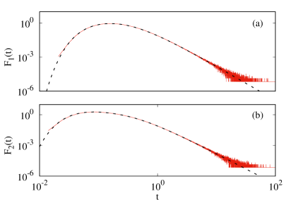
We test our analytical results by numerically estimating the conditional FPTDs for success and failure. We obtain these by numerically solving the Langevin equations

$$\dot{x}_{1} =\eta_{1}(t),$$ (5a)

$$\dot{x}_{2} =\eta_{2}(t).$$ (5b)

In (5), $\eta_{1}(t)$ and $\eta_{2}(t)$ are two independent Gaussian random deviates with mean zero and identical delta correlated variance, that is, $\langle\eta_{i}(t)\eta_{i}(t^{\prime})\rangle=2D\delta(t-t^{\prime})$ for $i=1,2$ with $D=1$. At $t=0$ the two walkers are at $x_{1}=1$ and $x_{2}=2$ and the process ends when either $x_{1}=0$ or $x_{1}=x_{2}$. Let $\mathcal{E}_{1}$ be the exit probability for the termination of the process by the first particle reaching the origin and $\mathcal{E}_{2}$ for the trajectories crossing each other. If $F_{1,n}(t)$ and $F_{2,n}(t)$ are the numerically estimated normalized histograms for the conditional first passage times, then $F_{i}(t)=\mathcal{E}_{i}F_{i,n}(t)$. We study this relation in Fig. 1 and find a good agreement between the analytical and numerical estimates of the conditional FPTDs.

Restarting the Bernoulli process: For reasons discussed in Ref. Singh and Singh (2022), we reset the two vicious walkers at the exact same moment. Furthermore, the time between two successive restarts is chosen for the purpose of simplicity to be either an exponentially distributed random variable (Poissonian resetting) or a fixed quantity (sharp resetting). If $T$ is the time of unconditional completion of the Bernoulli trial under consideration and $R$ is the time of restart of the process, then the probability of success is: $p=\frac{\langle I(T<R)y_{T}\rangle}{\langle I(T<R)\rangle}$ Belan (2018), where $y_{T}$ is an auxiliary random variable taking value one with probability $F_{1}(t)/F(t)$. Now, if $\langle T^{s}\rangle$ is the mean completion time of a successful trial then $\langle T^{s}\rangle=\frac{\langle I(T>R)R\rangle}{\langle I(T<R)\rangle}+\frac{\langle I(T<R)y_{T}T\rangle}{\langle I(T<R)y_{T}\rangle}$ Belan (2018). Let us now discuss Poisson and sharp restart protocols one by one.

Figure 2: Effect of Poisson restarts: (a) Numerically estimated probability of success $p_{r}$ (red circles) vs the analytical result from Eq. (6a) (black solid line). The black dashed line represents $\lim_{r\to 0}p_{r}$, success probability in absence of any restarts. (b) Numerically estimated mean time for a successful completion $\langle T^{s}_{r}\rangle$ (red circles) vs the analytical result from Eq. 6b (black solid line). Black dashed line represents $\lim_{r\to 0}\langle T^{s}_{r}\rangle$. Parameter values are $a_{1}=1,\leavevmode\nobreak\ a_{2}=2,\leavevmode\nobreak\ D=1$.

For Poissonian resetting at a rate $r$, the PDF of restart times is $P^{r}(R)=re^{-rR}$. As a result, the probability of success and the mean time for a successful completion respectively read Belan (2018):

$$p_{r} =\frac{\tilde{F_{1}}(r)}{\tilde{F}(r)},$$ (6a)

$$\langle T^{s}_{r}\rangle =\langle T_{r}\rangle-\frac{d}{dr}\ln p_{r},$$ (6b)

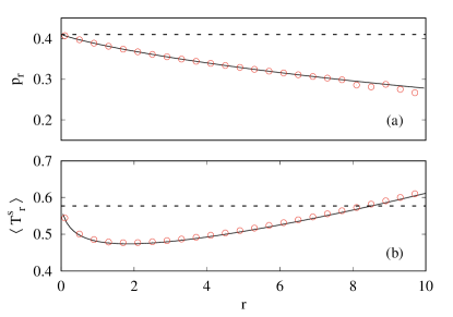
where $\langle T_{r}\rangle=\frac{1-\tilde{F}(r)}{r\tilde{F}(r)}$ Reuveni (2016) denotes the mean time of completion of the Bernoulli trial, either with a success or as a failure; and $\tilde{F}(r)=\int^{\infty}_{0}dt\leavevmode\nobreak\ e^{-rt}F(t)$ is the Laplace transform of $F(t)$. We compare these results for the capture problem against their numerical solution by solving Eq. (5) under Poissonian restarts at a rate $r$ and find good agreement between the two (see Fig. 2). It is evident from Fig.  2(a) that $p_{r}$ is a monotonically decreasing function of the restart rate $r$, while the mean time for successful completion $\langle T^{s}_{r}\rangle$ exhibits a minima, as seen from Fig. 2(b). This implies that while resetting makes it slightly less probable for the lamb to make it to the safe haven, the time to reach the safe haven can be minimal, for example, for $r\approx 2$. For higher values of restart rate like $r\approx 10$, the lamb is walking a slippery slope where it takes a longer time to reach the haven and the chances of it doing so are also severely diminished, thanks to the fact that it keeps returning home. It should be noted at this point that the Laplace transforms in Eq. (6) have been evaluated via numerical integration Press et al. (1986). Let us now move on to studying the Bernoulli trial under sharp resetting.

Figure 3: Effect of sharp restarts: (a) Numerically estimated probability of success $p_{\tau}$ (red circles) vs the analytical result from Eq. (7) (black solid line). The black dashed line represents $\lim_{\tau\to\infty}p_{\tau}$, success probability in absence of any restarts. (b) Numerically estimated mean time for a successful completion $\langle T^{s}_{\tau}\rangle$ (red circles) vs the analytical result from Eq. 8 (black solid line). Black dashed line represents $\lim_{\tau\to\infty}\langle T^{s}_{\tau}\rangle$. Parameter values are $a_{1}=1,\leavevmode\nobreak\ a_{2}=2,\leavevmode\nobreak\ D=1$.

For sharp resetting the PDF of restart times is $P^{\tau}(R)=\delta(R-\tau)$, where $\tau$ is the time of sharp restart. Then $\langle I(T<R)y_{T}\rangle=\int^{\infty}_{0}dR\leavevmode\nobreak\ P^{\tau}(R)\int^{\infty}_{0}dt\leavevmode\nobreak\ F(t)I(T<R)y_{T}=\int^{\infty}_{0}dt\leavevmode\nobreak\ F_{1}(t)\int^{\infty}_{t}dR\leavevmode\nobreak\ \delta(R-\tau)=\int^{\tau}_{0}dt\leavevmode\nobreak\ F_{1}(t)$ where we have reversed the order of integration in the second equality and the delta function term contributes only when $t\leq\tau$. In a similar manner we have $\langle I(T<R)\rangle=\int^{\tau}_{0}dt\leavevmode\nobreak\ F(t)$, from where follows the probability of success under sharp resetting

$$p_{\tau}=\frac{\int^{\tau}_{0}dt\leavevmode\nobreak\ F_{1}(t)}{\int^{\tau}_{0}dt\leavevmode\nobreak\ F(t)}.$$ (7)

Evaluating the remaining integrals we get $\langle I(T>R)R\rangle=\tau\int^{\infty}_{\tau}dt\leavevmode\nobreak\ F(t)$ and $\langle I(T<R)y_{T}T\rangle=\int^{\tau}_{0}dt\leavevmode\nobreak\ tF_{1}(t)$ leading to the mean time for a successful completion: $\langle T^{s}_{\tau}\rangle=\frac{\tau\int^{\infty}_{\tau}dt\leavevmode\nobreak\ F(t)}{\int^{\tau}_{0}dt\leavevmode\nobreak\ F(t)}+\frac{\int^{\tau}_{0}dt\leavevmode\nobreak\ tF_{1}(t)}{\int^{\tau}_{0}dt\leavevmode\nobreak\ F_{1}(t)}$ which can be re-written as

$$\langle T^{s}_{\tau}\rangle=\langle T_{\tau}\rangle-(1-p_{\tau})\frac{\int^{\tau}_{0}dt\leavevmode\nobreak\ tF_{2}(t)}{\int^{\tau}_{0}dt\leavevmode\nobreak\ F_{2}(t)}.$$ (8)

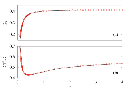
In the above equation, $\langle T_{\tau}\rangle=\frac{\int^{\tau}_{0}dt\leavevmode\nobreak\ tF(t)}{\int^{\tau}_{0}dt\leavevmode\nobreak\ F(t)}+\frac{\tau\int^{\infty}_{\tau}dt\leavevmode\nobreak\ F(t)}{\int^{\tau}_{0}dt\leavevmode\nobreak\ F(t)}$ is the mean time of completion of the Bernoulli trial in presence of sharp resetting and $F_{2}(t)$ is defined in Eq. (4). It is interesting to see the close analogy between the equations for Poisson and sharp restarts. We now compare the analytical results of Eq. (7) and (8) with numerical solution of the Langevin equations (5) under sharp resetting and find excellent agreement between the two approaches in Fig. 3. Furthermore, the success probability under sharp restarts $p_{\tau}$ asymptotically approaches its value in absence of any restarts in a monotonic way and remains less than $\lim_{\tau\to\infty}p_{\tau}$ (see Fig. 3(a)). On the other hand, the mean time taken by the lamb to successfully reach the safe haven $\langle T^{s}_{\tau}\rangle$ exhibits a non-monotonic dependence (in sharp contrast with $p_{\tau}$) on the restart time $\tau$. This implies that sharp resetting is advantageous for the lamb as it is able to quickly take resort to the safe haven as compared to the case when there are no restarts. Unlike its Poissonian counterpart, a sharp restart of the Bernoulli trial with high value of $\tau$ is advantageous for the lamb, as its probability to make it to the safe haven is close to $\mathcal{E}_{1}$, and this mode of completion takes a lesser amount of time on average. This prompts us to make an explicit comparison between the two restart protocols, and more so their relation to the dynamics of the Bernoulli trial without restarts. We proceed with this goal in the next section.

Comparing Poissonian restart with sharp restart:

Figure 4: Comparing success probability for Poisson and sharp restarts. Inset shows the behavior at very large rates. Here the rate $\rho$ denotes either $r$ or $1/\tau$ depending on the restart protocol under consideration, viz. Poisson or sharp, respectively. Parameter values are $a_{1}=1,\leavevmode\nobreak\ a_{2}=2,\leavevmode\nobreak\ D=1$.

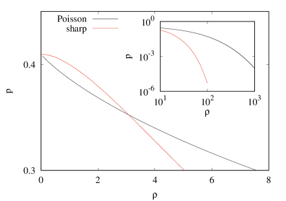
In order to compare Poissonian and sharp restart for the Bernoulli trial under consideration, let us define $1/\tau$ as the rate of sharp restart, where $\tau$ is the time of sharp restart. This definition puts the two restart protocols on same footing and we define $\rho$ as the rate of restart, with $\rho=r$ for Poisson restart and $\rho=1/\tau$ for sharp restart. As we have seen above, for both Poisson and sharp restart protocols, we have $\lim_{r\to 0}p_{r}=\lim_{\tau\to\infty}{p_{\tau}}=\mathcal{E}_{1}$. This is also seen in Fig. 4 for $\rho$ in the neighborhood of zero. However, the approach of $p_{r}$ and $p_{\tau}$ to $\mathcal{E}_{1}$ is completely different in that the second derivative $d^{2}p/d\rho^{2}$ near $\rho\approx 0$ is positive or negative depending on whether we consider Poisson or sharp restart protocol (see Fig. 4). This can be understood as follows. For sharp restart $\rho$ near zero means that the time interval between two successive restarts $\tau$ is very large, which means that the Bernoulli trial stops without being practically perturbed by any restart event (see the near horizontal behavior of $p$ for small $\rho$ in Fig. 4). On the other hand, since $\langle T\rangle<\langle T^{s}\rangle$ (from Eqs. (Escape of a lamb to safe haven in pursuit by a lion under restarts) and (4a)), we have for Poissonian restarts: $p_{r}\stackrel{{\scriptstyle r\to 0}}{{\sim}}\mathcal{E}_{1}+\mathcal{E}_{1}(\langle T\rangle-\langle T^{s}\rangle)r$, which leads to $dp_{r}/dr<0$ for $r\to 0$. Note that we can take this analysis no further as the higher order moments of the FPTD $F(t)$ do not exist. The difference in the signs of the second derivative of success probability eventually lead to $p_{\tau}<p_{r}$ for large $\rho$ with $\lim_{\rho\to\infty}p=0$ (see inset in Fig. 4). This follows simply from the fact that for large $\rho$ both the vicious walkers are reset to their initial locations very rapidly, making it practically impossible for the lamb to make it to the safe haven. However, the fact that lion is also going to its den every now and then, makes the mean time taken by the lamb to reach the safe have extremely large (see Figs. 2 and 3 for a comparison).

Figure 5: Comparing the FPTDs $F_{r}(t)$ and $F_{\tau}(t)$ under Poissonian (red) and sharp (blue) restarts respectively. The symbols are numerically estimated and the dashed lines represent the analytical approximations obtained via inverting the Laplace representations. The periodic behavior of $F_{\tau}(t)$ is evident. Parameter values are $a_{1}=1,\leavevmode\nobreak\ a_{2}=2,\leavevmode\nobreak\ D=1$.

Let us now discuss the effect of resetting on the FPTD $F(t)$. Under Poissonian resetting at a rate $r$, the FPTD is known to be: $\tilde{F}_{r}(s)=\frac{\tilde{F}(s+r)}{\frac{s}{s+r}+\frac{r}{s+r}\tilde{F}(s+r)}$ Reuveni (2016) and from here follows the FPTD under Poissonian resetting via the Bromwich integral Arfken and Weber (1999):

$$F_{r}(t)=\frac{1}{2\pi i}\int^{\gamma+i\infty}_{\gamma-i\infty}ds\leavevmode\nobreak\ \frac{(s+r)\tilde{F}(s+r)}{s+r\tilde{F}(s+r)}e^{st}.$$ (9)

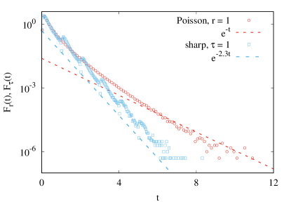
While an exact evaluation of the above integral is difficult, we can obtain the long-time behavior of $F_{r}(t)$ by looking at the pole of $\tilde{F}_{r}(s)$ closest to the origin. If $s_{0,r}$ is the pole nearest to zero, then it solves the equation: $0=s+r\mathcal{L}[e^{-rt}F(t)]$, where $\mathcal{L}$ denotes Laplace transform. We evaluate the Laplace transform for a specific value of $r=1$, and by numerically estimating $\mathcal{L}[e^{-rt}F(t)]$ we find $s_{0,r}\approx-1.0$. As a result, for $t\gg 1$ we have $F_{r}(t)\approx e^{-s_{0,r}t}$. We compare this approximate result in Fig. 5, wherein we estimate $F_{r}(t)$ by numerically solving the Langevin equations in (5) under Poissonian resetting with $r=1$. It is evident from the figure that we have a reasonable agreement between the analytical and numerical estimates, though we would not call it good. The reason for this difference is that numerical estimations suggest $F_{r}(t)\approx e^{-1.25t}$, which is an error of about $20\%$ when compared to the analytical approximation $F_{r}(t)\approx e^{-t}$. With an exact representation of the Laplace transform $\tilde{F}(s)$ unavailable, we cannot provide a plausible explanation for this difference here.

For sharp resetting, the FPTD in Laplace domain reads Pal and Reuveni (2017); Singh and Singh (2022):

$$\tilde{F}_{\tau}(s)=\frac{\int^{\tau}_{0}dt\leavevmode\nobreak\ F(t)e^{-st}}{1-e^{-s\tau}\int^{\infty}_{\tau}dt\leavevmode\nobreak\ F(t)},$$ (10)

and its Laplace inversion at long times is determined by the pole $s_{0,\tau}$ of $\tilde{F}_{\tau}(s)$ closest to zero. It is given by the solution of the equation: $0=1-e^{-s_{0,\tau}\tau}\int^{\infty}_{\tau}dt\leavevmode\nobreak\ F(t)\Rightarrow s_{0,\tau}=\frac{1}{\tau}\log\Big{(}\int^{\infty}_{\tau}dt\leavevmode\nobreak\ F(t)\Big{)}$. For a specific value like $\tau=1$ results in $s_{0,\tau}\approx-2.3$ which, at large times leads to $F_{\tau}(t)\approx e^{-s_{0,\tau}t}$. Let us now look at the properties of $\tilde{F}_{\tau}(s)$ in some more detail. The defining property of sharp resetting is that it introduces a periodicity in the system, with the period being $\tau$, the time interval between two sharp restarts. Furthermore, if we consider a periodic function with a period $\tau$, that is, $h(t+\tau)=h(t)$, then its Laplace transform reads Spiegel (1965); Schiff (1999):

$$\tilde{h}(s)=\frac{\int^{\tau}_{0}dt\leavevmode\nobreak\ h(t)e^{-st}}{1-e^{-s\tau}}.$$ (11)

A quick look at Eqs. (10) and (11) shows the degree of their similarity, except for the appearance of the term $\int^{\infty}_{\tau}dt\leavevmode\nobreak\ F(t)$ in the denominator of the fraction defining $\tilde{F}_{\tau}(s)$ in Eq. (10). Now, with the information that $F_{\tau}(t)\approx e^{-s_{0,\tau}t}$ for large $t$, we can discern that the FPTD $F_{\tau}(t)$ has a periodic structure (with period $\tau$) and its envelope decaying exponentially. It is to be noted at this point that this behavior of the FPTD is generic to any first passage process under sharp resetting, and not limited to the Bernoulli trial under consideration. For the Bernoulli trial, however, we can make a comparison of our analytical approximation against numerical calculations. We see from Fig. 5 that $F_{\tau}(t)$ does exhibit a periodic behavior with an envelope tracing the curve $F_{\tau}(t)\approx e^{-2.3t}$ (obtained via Laplace inversion). Furthermore, the period of the FPTD $F_{\tau}(t)$ is $\tau=1$, as explained above.

It is to be noted that we have studied the Bernoulli trial problem under restarts for parameter values $(a_{1},a_{2},D)=(1,2,1)$, though we checked for other parameter values like $(a_{1},a_{2},D)=(1/2,2,1)$ and found similar behavior. It is for this reason that we report only the former set of parameters.

Conclusions: If we ask ourselves one question, what is the quintessential problem in life, we shall almost always come to one answer: the problem is choice. Motivated by this line of thought, we study the capture problem wherein a hungry lion pursues a lamb in presence of a safe haven for the lamb. This is one of the classic problems in nonequilibrium statistical physics, and presents us with an example of a first passage process which can terminate in two ways: either the lamb reaches the safe haven (success) or is killed by the lion (failure). Following the seminal work of Fisher Fisher (1984), we are able to obtain the exact solution for the two-particle problem. We find that the distribution of first passage times possesses a finite mean, though no higher moments exist. We further study this problem under Poissonian and sharp restarts, and find that the probability of success exhibits a monotonic dependence on the rate of restart for Poissonian restart, or the time of sharp restart. In addition, the FPTDs under restarts exhibit exponentially decaying tails, and we find a reasonable agreement between the analytical approximations and the numerical estimates.

The importance of capture problems, and a limited amount of literature studying Bernoulli trials under restarts makes this study a timely work. While we have chosen two identical Brownian particles, going to a set of non-identical but vicious walkers (different diffusion coefficients $D_{1}$ and $D_{2}$) is straightforward. However, the more interesting cases wherein the walkers are either a pair of vicious run and tumble particles Le Doussal et al. (2019) or a run and tumble particle viciously interacting with another Brownian particle are worth considering.

Acknowledgments: RKS thanks the Israel Academy of Sciences and Humanities (IASH) and the Council of Higher Education (CHE) Fellowship. TS acknowledges financial support by the German Science Foundation (DFG, Grant number ME 1535/12-1). TS is supported by the Alliance of International Science Organizations (Project No. ANSO-CR-PP-2022-05). TS is also supported by the Alexander von Humboldt Foundation. SS thanks Kreitman Fellowship and HPC facility at Ben-Gurion University.

References

- Krapivsky et al. (2010) P. L. Krapivsky, S. Redner, and E. Ben-Naim, A kinetic view of statistical physics (Cambridge University Press, 2010).
- Bernardi and Lindner (2022) D. Bernardi and B. Lindner, Phys. Rev. Lett. 128, 040601 (2022).
- Elgart and Kamenev (2004) V. Elgart and A. Kamenev, Phys. Rev. E 70, 041106 (2004).
- Assaf and Meerson (2006) M. Assaf and B. Meerson, Phys. Rev. E 74, 041115 (2006).
- Assaf and Meerson (2007) M. Assaf and B. Meerson, Phys. Rev. E 75, 031122 (2007).
- Khasin and Dykman (2009) M. Khasin and M. I. Dykman, Phys. Rev. Lett. 103, 068101 (2009).
- Nayak et al. (2020a) I. Nayak, D. Das, and A. Nandi, Phys. Rev. Research 2, 013114 (2020a).
- Fisher (1984) M. E. Fisher, J. Stat. Phys. 34, 667 (1984).
- Huse and Fisher (1984) D. A. Huse and M. E. Fisher, Phys. Rev. B 29, 239 (1984).
- Ispolatov et al. (1996) I. Ispolatov, P. L. Krapivsky, and S. Redner, Phys. Rev. E 54, 1274 (1996).
- Bray et al. (2013) A. J. Bray, S. N. Majumdar, and G. Schehr, Adv. Phys. 62, 225 (2013).
- Forrester (1989) P. J. Forrester, J. Stat. Phys. 56, 767 (1989).
- Katori and Tanemura (2002) M. Katori and H. Tanemura, Phys. Rev. E 66, 011105 (2002).
- Baik (2000) J. Baik, Commun. Pure Appl. Math.: A Journal Issued by the Courant Institute of Mathematical Sciences 53, 1385 (2000).
- Essam and Guttmann (1995) J. W. Essam and A. J. Guttmann, Phys. Rev. E 52, 5849 (1995).
- Pedersen et al. (2009) J. N. Pedersen, M. S. Hansen, T. Novotnỳ, T. Ambjörnsson, and R. Metzler, J. Chem. Phys. 130, 164117 (2009).
- Cardy and Täuber (1996) J. Cardy and U. C. Täuber, Phys. Rev. Lett. 77, 4780 (1996).
- Fisher and Gelfand (1988) M. E. Fisher and M. P. Gelfand, J. Stat. Phys. 53, 175 (1988).
- Schehr et al. (2008) G. Schehr, S. N. Majumdar, A. Comtet, and J. Randon-Furling, Phys. Rev. Lett. 101, 150601 (2008).
- Kundu et al. (2014) A. Kundu, S. N. Majumdar, and G. Schehr, J. Stat. Phys. 157, 124 (2014).
- Cardy and Katori (2003) J. Cardy and M. Katori, J. Phys. A: Math. Gen. 36, 609 (2003).
- Krapivsky and Redner (1996) P. L. Krapivsky and S. Redner, J. Phys. A: Math. Gen. 29, 5347 (1996).
- Redner and Krapivsky (1999) S. Redner and P. L. Krapivsky, Amer. J. Phys. 67, 1277 (1999).
- Nayak et al. (2020b) I. Nayak, A. Nandi, and D. Das, Phys. Rev. E 102, 062109 (2020b).
- Oshanin et al. (2009) G. Oshanin, O. Vasilyev, P. L. Krapivsky, and J. Klafter, Proc. Natl. Acad. Sci. U.S.A. 106, 13696 (2009).
- Redner (2001) S. Redner, A guide to first-passage processes (Cambridge university press, 2001).
- Redner and Bénichou (2014) S. Redner and O. Bénichou, J. Stat. Mech.: Theor. Exp. 2014, P11019 (2014).
- Ben-Avraham et al. (2003) D. Ben-Avraham, B. M. Johnson, C. A. Monaco, P. L. Krapivsky, and S. Redner, J. Phys. A: Math. Gen. 36, 1789 (2003).
- Klafter and Sokolov (2011) J. Klafter and I. M. Sokolov, First steps in random walks: from tools to applications (OUP Oxford, 2011).
- Weiss and Rubin (1983) G. H. Weiss and R. J. Rubin, Adv. Chem. Phys. 52, 363 (1983).
- Gabel et al. (2012) A. Gabel, S. N. Majumdar, N. K. Panduranga, and S. Redner, J. Stat. Mech.: Theor. Exp. 2012, P05011 (2012).
- Feller (1971) W. Feller, An introduction to probability theory and its applications, Tech. Rep. (Wiley series in probability and mathematical statistics, 3rd edn.(Wiley, New York), 1971).
- Edwards (1983) A. W. F. Edwards, Int. Stat. Rev. 51, 73 (1983).
- Condamin et al. (2007) S. Condamin, O. Bénichou, and M. Moreau, Phys. Rev. E 75, 021111 (2007).
- Condamin et al. (2008) S. Condamin, V. Tejedor, R. Voituriez, O. Bénichou, and J. Klafter, Proc. Natl. Acad. Sci. U.S.A. 105, 5675 (2008).
- Benichou et al. (2015) O. Benichou, T. Guérin, and R. Voituriez, J. Phys. A: Math. Theor. 48, 163001 (2015).
- Lohmar and Krug (2009) I. Lohmar and J. Krug, J. Stat. Phys. 134, 307 (2009).
- Abad et al. (2012) E. Abad, S. B. Yuste, and K. Lindenberg, Phys. Rev. E 86, 061120 (2012).
- Yuste et al. (2013) S. B. Yuste, E. Abad, and K. Lindenberg, Phys. Rev. Lett. 110, 220603 (2013).
- Campos et al. (2015) D. Campos, E. Abad, V. Méndez, S. B. Yuste, and K. Lindenberg, Phys. Rev. E 91, 052115 (2015).
- Meerson and Redner (2015) B. Meerson and S. Redner, Phys. Rev. Lett. 114, 198101 (2015).
- Rehbein and Carpenter (2011) J. Rehbein and B. K. Carpenter, Phys. Chem. Chem. Phys. 13, 20906 (2011).
- Solomatin et al. (2010) S. V. Solomatin, M. Greenfeld, S. Chu, and D. Herschlag, Nature 463, 681 (2010).
- Pierse and Dudko (2017) C. A. Pierse and O. K. Dudko, Phys. Rev. Lett. 118, 088101 (2017).
- Belan (2018) S. Belan, Phys. Rev. Lett. 120, 080601 (2018).
- Evans and Majumdar (2011) M. R. Evans and S. N. Majumdar, Phys. Rev. Lett. 106, 160601 (2011).
- Evans and Majumdar (2018) M. R. Evans and S. N. Majumdar, J. Phys. A: Math. Theor. 51, 475003 (2018).
- Gupta et al. (2014) S. Gupta, S. N. Majumdar, and G. Schehr, Phys. Rev. Lett. 112, 220601 (2014).
- Majumdar et al. (2015) S. N. Majumdar, S. Sabhapandit, and G. Schehr, Phys. Rev. E 91, 052131 (2015).
- Singh et al. (2022) R. K. Singh, K. Gorska, and T. Sandev, Phys. Rev. E 105, 064133 (2022).
- Ahmad et al. (2019) S. Ahmad, I. Nayak, A. Bansal, A. Nandi, and D. Das, Phys. Rev. E 99, 022130 (2019).
- Ahmad et al. (2022) S. Ahmad, K. Rijal, and D. Das, Phys. Rev. E 105, 044134 (2022).
- Masoliver (2019) J. Masoliver, Phys. Rev. E 99, 012121 (2019).
- Domazetoski et al. (2020) V. Domazetoski, A. Masó-Puigdellosas, T. Sandev, V. Méndez, A. Iomin, and L. Kocarev, Phys. Rev. Research 2, 033027 (2020).
- Singh et al. (2021) R. K. Singh, T. Sandev, A. Iomin, and R. Metzler, J. Phys. A: Math. Theor. 54, 404006 (2021).
- Evans and Majumdar (2014) M. R. Evans and S. N. Majumdar, J. Phys. A: Math. Theor. 47, 285001 (2014).
- Pal et al. (2022) A. Pal, S. Kostinski, and S. Reuveni, J. Phys. A: Math. Theor. 55, 021001 (2022).
- Pal et al. (2016) A. Pal, A. Kundu, and M. R. Evans, J. Phys. A: Math. Theor. 49, 225001 (2016).
- Pal and Reuveni (2017) A. Pal and S. Reuveni, Phys. Rev. Lett. 118, 030603 (2017).
- Chechkin and Sokolov (2018) A. Chechkin and I. M. Sokolov, Phys. Rev. Lett. 121, 050601 (2018).
- Eliazar and Reuveni (2020) I. Eliazar and S. Reuveni, J. Physics A: Math. Theor. 53, 405004 (2020).
- Eliazar and Reuveni (2021a) I. Eliazar and S. Reuveni, J. Phys. A: Math. Theor. 54, 355001 (2021a).
- Eliazar and Reuveni (2021b) I. Eliazar and S. Reuveni, J. Phys. A: Math. Theor. 54, 125001 (2021b).
- Eliazar and Reuveni (2022a) I. I. Eliazar and S. Reuveni, J. Phys. A: Math. Theor. 56, 024002 (2022a).
- Eliazar and Reuveni (2022b) I. I. Eliazar and S. Reuveni, J Phys. A: Math. Theor. 56, 024003 (2022b).
- Pal and Prasad (2019) A. Pal and V. Prasad, Phys. Rev. E 99, 032123 (2019).
- Singh and Singh (2022) R. K. Singh and S. Singh, Phys. Rev. E 106, 064118 (2022).
- Reuveni (2016) S. Reuveni, Phys. Rev. Lett. 116, 170601 (2016).
- Press et al. (1986) W. H. Press, S. A. Teukolsky, W. T. Vetterling, and B. P. Flannery, Numerical Recipes in Fortran 77 (Cambridge university press Cambridge, 1986).
- Arfken and Weber (1999) G. B. Arfken and H. J. Weber, “Mathematical methods for physicists,” (1999).
- Spiegel (1965) M. R. Spiegel, Theory and problems of Laplace transforms (McGraw-Hill New York, 1965).
- Schiff (1999) J. L. Schiff, The Laplace transform: theory and applications (Springer Science & Business Media, 1999).
- Le Doussal et al. (2019) P. Le Doussal, S. N. Majumdar, and G. Schehr, Phys. Rev. E 100, 012113 (2019).