A search for the missing baryons with X–ray absorption lines towards the blazar

Abstract

This paper presents an analysis of XMM-Newton X–ray spectra of the quasar 1ES 1553+113, in search for absorption lines from the intervening warm–hot intergalactic medium. A search for O VII, O VIII and Ne IX resonance absorption lines was performed at eight fixed redshifts that feature O VI or H I broad Lyman–$\alpha$ absorption lines that were previously detected from HST data The search yielded one possible detection of O VII at a redshift $z\simeq 0.1877$ with an O VI prior, with a statistical significance that is equivalent to a 2.6–$\sigma$ confidence level. The spectra were also stacked at the wavelengths of the expected redshifted O VII and O VIII lines, but the analysis did not reveal evidence for the presence of additional X–ray absorbing WHIM. Moreover, the spectra were used to investigate two putative O VII absorption lines that were detected serendipitously in an earlier analysis of the same data by F. Nicastro and collaborators. The paper also presents a comprehensive statistical framework for cosmological inferences from the analysis of absorption lines, which makes use of cosmological simulations for the joint probability distributions of FUV and X–ray ions. Accordingly, we conclude that the new possible O VII absorption at $z\simeq 0.1877$ is consistent with a contribution from the hot WHIM to the baryon density in an amount of $\Omega_{\mathrm{WHIM,X}}/\Omega_{b}=44\pm 22$%. However, there are large systematic uncertainties associated with the temperature and abundances of the absorbers, and only a larger sample of X-ray sources can provide an accurate determination of the cosmological density of the WHIM.

1 Introduction

One of cosmology’s open questions is the location of a fraction of the ordinary baryonic matter in the local universe. This issue, commonly referred to as the missing baryons problem, arises from the comparison between high–redshift detections of baryons, primarily via the Lyman-$\alpha$ forest, and measurements at low redshift, whereas a sizable fraction of the high–redshift baryons appear to be unaccounted for in the low–redshift universe (Shull et al., 2012). For over two decades, numerical simulations have suggested that the missing baryons may be located in filamentary structures of galaxies that host a warm–hot intergalactic medium at temperatures of approximately $\log T(K)=5-7$ (the WHIM, e.g. Cen & Ostriker, 1999; Davé et al., 2001; Bertone et al., 2008; Cautun et al., 2014; Martizzi et al., 2018; Tuominen et al., 2021). The lower range of WHIM temperatures has been effectively probed with FUV absorption lines by FUSE and HST, revealing a number of absorption lines in the spectra of background sources, primarily H I broad Lyman–$\alpha$ (BLA), O VI, C IV, and other lines. Such FUV absorption lines are likely to arise either from warm–hot gas in the the outer regions of individual galaxies or from the intergalactic WHIM, and they track a significant fraction of the low–redshift baryons (e.g. Tilton et al., 2012; Shull et al., 2012; Stocke et al., 2014; Danforth et al., 2016). The higher range of WHIM temperatures have been more challenging to probe, primarily because the most prominent absorption lines associated with a plasma at $\log T(K)\geq 6$ are in the X–ray range (i.e., the O VII and O VIII resonance lines), and the available spectrometers on board XMM-Newton and Chandra are not as sensitive at the FUV instruments.

Despite the challenges associated with the flux of available background sources and the resolutions and sensitivity of the X–ray spectrometers, a few detections of absorption lines from the WHIM have been reported, including two in the spectrum of the quasar 1ES 1553+113 (Nicastro et al., 2018; Nicastro, 2018), which is the subject of the present investigation. Other detections of the WHIM through X–ray absorption include PKS 2155-304 (Fang et al., 2002; Fang et al., 2007), although the detection was not confirmed by others (Yao et al., 2009; Cagnoni et al., 2004; Nevalainen et al., 2019); Mrk 421 by Nicastro et al. (2005), which was however followed by reports of non–detections by Rasmussen et al. (2007) and Yao et al. (2012); in H 2356-309 by Fang et al. (2010) and Buote et al. (2009); in Mrk 501 by Ren et al. (2014), in Ton S180 (Ahoranta et al., 2021) and in 3C 273 (Ahoranta et al., 2020), and finally in PG 1116+215 by Bonamente et al. (2016); Bonamente et al. (2019). Finally, a tentative detection in H 1821+643 was reported by Kovács et al. (2019) using stacking of signals at different redshifts, using a method that is similar to the one used in this paper.

The study of EAGLE hydrodynamical simulations by Wijers et al. (2019) suggests that there is significant correlation between O VI and H I BLA FUV absorption lines and prominent X–ray ions such as O VII and O VIII. This correlation motivates our search for X–ray counterparts to FUV absorption lines in the spectrum of 1ES 1553+113, and of other sources with FUV detections reported by the HST and FUSE surveys of Tilton et al. (2012) and Danforth et al. (2016). In this paper we present the results of our search for 1ES 1553+113, and develop the method of analysis that will be used for a larger sample of FUV sources, including the use of systematic upper limits to the non–detection of X–ray lines.

This paper is structured as follows: in Section 2 we describe our strategy for the search of X–ray absorption lines and the available FUV absorption data towards 1ES 1553+113, in Section 3 the available X–ray data used for this investigation, in Section 4 our analysis of the search and analysis of the X–ray absorption lines. Finally, Sect. 5 presents the cosmological implication of the results, and Section 6 a discussion and the conclusions.

2 The search for X–ray absorption towards 1ES 1553+113

Nicastro et al. (2018) conducted a blind search for X-ray absorption lines in the XMM-Newton spectrum of the X–ray bright blazar 1ES 1553+113, and identified two absorption features interpreted as O VII He–$\alpha$ absorbers at $z\simeq 0.4339$ and 0.3557 possibly associated with the WHIM towards the blazar. At those redshifts, there are a handful of galaxies with confirmed redshifts that are at a projected distance of $\leq 1.5$ Mpc from the sightline and with a velocity within 1,000 km s^-1 of the X-ray redshifts. These galaxies might be indicative of the presence of a filamentary structure that may host WHIM gas, but no filament detection was attempted to confirm it.

2.1 The redshift of 1ES 1553+113

Unfortunately, the spectroscopic redshift of 1ES 1553+113 is unknown, because its spectrum lacks intrinsic emission or absorption lines usually employed to measure it. Based on intervening Lyman-$\alpha$  FUV absorption, Danforth et al. (2010); Danforth et al. (2016) constrained its redshift to a range $0.413<z<0.56$, and possibly with a value of $z=0.49\pm 0.04$, based on $\gamma$–ray observations (Abramowski et al., 2015). These measurements were used by Nicastro et al. (2018) to suggest a WHIM origin for the two serendipitous absorption lines they detected.

A recent study by Dorigo Jones et al. (2022) constrains the redshift of several of these nearly featureless BL Lac blazars, which constitute a significant fraction of all blazars. The study also includes new near-UV observations of 1ES 1553+113 that were not available at the time of the Nicastro et al. (2018) paper. Based on the maximum redshift of the intervening Lyman-$\alpha$ forest towards 1ES 1553+113 ($z=0.4131$), the distribution of the difference between the spectroscopic redshifts and the maximum Lyman-$\alpha$  redshift from other blazars (including the X–ray–bright 3C 273, PKS 2155-304 and Mkn 421) indicates a 95% probability that the redshift of 1ES 1553+113 is in the range $0.408<z<0.436$. Moreover, Johnson et al. (2019) had shown that 1ES 1553+113 is likely a member of a group of galaxies located near $z=0.433$.

The combination of these results suggests that the most likely redshift for 1ES 1553+113 is approximately $z\simeq 0.433$, in correspondence of the strongest of the two Nicastro et al. (2018) absorption lines. If this is correct, then the putative O VII $z\simeq 0.4339$ absorption would be intrinsic to the source, and not associated with the WHIM. For the main purpose of this paper, which is to investigate X–ray absorption lines at FUV–prior redshifts, the $z=0.4131$ Lyman-$\alpha$  absorption towards 1ES 1553+113 sets a clear lower limit for the redshift of the blazar, $z\geq 0.4131$, and therefore the search for absorption lines at redshifts that are lower than this limit is warranted. In Sects. 4 and 5 we will further discuss the uncertainties associated with the lack of a spectroscopic redshift for 1ES 1553+113.

2.2 The Search for the WHIM with FUV priors

The search for WHIM X–ray absorption lines can be aided by the presence of FUV absorption lines that may act as sign–posts for the higher–temperature ions, instead of performing a blind search at all redshifts. The strategy we employ is to use O VI or H I BLA detections to identify reliable absorption line systems, and then using the X–ray spectra to search for possible counterparts (such as O VII and O VIII) associated with the FUV ions, as pioneered by Bonamente et al. (2016) and Nevalainen et al. (2019). The assumption of this search method is that the WHIM is multi–phase, and that lower–temperature ions provide a prior for the redshift that increases the statistical significance and the overall credibility of any associated X–ray detection. This assumption is consistent with the positive detections we have previously reported for 3C 273, Ton S180 and PG 1116+215 (Ahoranta et al., 2020, 2021; Bonamente et al., 2016). The use of FUV ions as indicators for O VII and O VIII is also suggested by the analysis of EAGLE simulations by Wijers et al. (2019), who finds significant correlation between both O VI and H I  absorption with both O VII and O VIII. In particular, the strongest correlation is between either the Ne VIII and O VI FUV ions, and the O VII X–ray ion, while the correlation between H I and X–ray ions is lower (see Fig. 14 of Wijers et al. 2019).

Our method consists of the analysis of the following FUV absorption–line systems:
(a) O VI detections where both lines in the $\lambda\lambda$ 1031.9, 1037.6 Å doublet are detected, in such a way that the identification of the FUV signal as the O VI doublet is secure; and
(b) H I Lyman-$\alpha$ with broadening $b\geq 40$ km s^-1, indicative of hydrogen at $\log T(K)\geq 5$ (as in Nevalainen et al. 2019), which marks the typical boundary for WHIM gas.

Towards 1ES 1553+113, the relevant FUV absorption lines from the Danforth et al. (2016) catalog are reported in Table 4, for a total of 8 FUV absorption line systems that meet our criteria as possible sign–posts for higher–energy X–ray ions. All of the FUV redshifts are lower than the minimum source redshift discussed in the previous section ($z\geq 0.4131$). The first two detected O VI systems are separated by $\Delta z=0.0002$, or a velocity of 60 km s^-1, which cannot be resolved by the X–ray spectrometers, and therefore they will be treated as a single system for the sake of the X–ray search. This is the same search method by which we identified two possible X–ray WHIM systems in PG 1116+215 and in Ton S180 (Bonamente et al., 2016; Ahoranta et al., 2021) that are counterparts of FUV detections, in addition to lower–significance signals in the spectra of 3C 273 and PKS 2155-304 (Ahoranta et al., 2020; Nevalainen et al., 2019).

3 X-ray data

This paper uses data from the XMM-Newton RGS and Chandra LETG grating spectrometers. The methods of analysis of the X–ray data follows those presented in Nevalainen et al. (2017) and Ahoranta et al. (2020) for XMM-Newton, and in Bonamente et al. (2016) for Chandra. In the following we summarize the main features of the data and data processing.

3.1 Processing

3.1.1 XMM-Newton/RGS

We analyzed all RGS observations of 1ES1553+113 available as of May 2022, for a total of 23 observations  with total RGS exposure time of $\sim 1.8$ Ms. The observations are reported in Table 1.

Table 1: Log of XMM-Newton and Chandra observations of 1ES 1553+113

Obs ID	Exp. time (s)
XMM-Newton
0094380801	4374
0656990101	21815
0727780101	33307
0727780201	35001
0727780301	28605
0727780401	28701
0727780501	28190
0727780601	25482
0761100101	136312
0761100201	132836
0761100301	137321
0761100401	131393
0761100701	88618
0761101001	131870
0790380501	96482
0790380601	102300
0790380801	113713
0790380901	129190
0790381001	91261
0790381401	123553
0790381501	138104
0810830101	31039
0810830201	28360
Total	1,817,827
Chandra
12915	166307
12916	153935
12917	175403
Total	495,645

We used the XMM-Newton SAS 18.0.0 software with the most recent calibration files available on July 2020 (XMM-CCF-REL-378) for processing the first order data. The data were reduced with the rgsproc pipeline using mostly the standard parameter values, except what is discussed below. In general, we follow the processing procedure laid out in Ahoranta et al. (2020). Radiation damage caused by cosmic rays induces local enhancement of dark current, or extra charge traps (de Vries et al., 2014), which manifest themselves as hot and cool pixels (i.e. bad pixels). Permanent bad pixels have been mapped by the RGS team and the information on their location etc. is included in the calibration files. The standard processing with default parameters uses this information to reject the data from hot pixels but not from the cool pixels. Following Ahoranta et al. (2020), we employed the recent option keepcool=no to also reject the data from cool pixels. In addition, time-variable bad pixels not rejected by the standard pipeline may affect the given observation, and they were removed upon visual inspection of the spectra.

The spectra were extracted with a 10 mÅ bin size, and then rebinned to 20 mÅ for the analysis. We then co-added the first-order spectra from different observations, keeping RGS1 and RGS2 separate, using the rgscombine procedure. These co-added spectra were then converted into the SPEX format using the trafo (version 1.04) software.

3.1.2 Chandra/LETG/HRC

The Chandra data were processed with CIAO 4.11 using the standard processing pipeline chandra_repro. The 3 HRC observations available for 1ES 1553+113 are listed in Table 1. For each observation, we combined the $\pm 1$ order LETG grating spectra into a single spectrum. The spectra were then combined into a single spectrum for analysis with SPEX using the same trafo software used for the analysis of XMM-Newton data. Additional details on the data reduction methods are in Bonamente et al. (2016).

3.2 Sensitivity of the data for the detection of absorption lines

Before embarking on a study of a large number of relatively weak absorption lines, we investigated the constraints set by statistical and systematic uncertainties. The RGS1 and RGS2 1st order effective area calibration uncertainties have been estimated as $\sim$2% in the 10–30 Å band, except for certain regions (such as near the oxygen edge) where 3-5% uncertainties may occur (Kaastra et al., 2018). The uncertainties in the calibration of the effective area for the LETG/HRC instruments have been estimated at $\leq 10$% across the entire band.

In order to evaluate the effect of possible effective area calibration inaccuracy on our results, we approximated the effect as a 2% dip in the predicted continuum flux within a bin of 60 mÅ size, i.e. the RGS resolution element, relative to the surrounding continuum. This is intended as a means to model a typical scenario in which a mis–calibrated effective area leads to a spurious absorption line–like feature. We then modelled this feature with a Gaussian line model (line in SPEX) with a broadening of 100 km/s at a nominal wavelength of 20 Å, and found that this feature requires a value of the optical depth parameter $\tau_{0}$= 0.37, producing an absorption line with equivalent width of EW_sys = 2.7 mÅ. This corresponds to $\log N_{\text{ion}}$ (cm${}^{-2})\simeq 15.0$, using a slab model for an He–$\alpha$ O VII absorption line. This is an indication that typical systematic uncertainties do not permit the detection of O VII column densities less that approximately $\log N_{\mathrm{OVII}}$ (cm${}^{-2})=15.0$. For the Chandra HRC data, a 10% uncertainty in the effective area in a resolution element of $\sim$60 mÅ corresponds to a value of $\tau_{0}$= 1.1, and it results in the inability to detect absorption lines with below EW_sys = 14 mÅ. In turn, this corresponds to an O VII column density of $\log N_{\text{ion}}$ (cm${}^{-2})\simeq 15.7$, following the same analysis as for the XMM-Newton data.

We then calculated the relative statistical uncertainties of the RGS and HRC spectra, using the background-subtracted count rate and its statistical uncertainty within each resolution element across the full waveband of the data. We then converted the relative statistical uncertainties into the equivalent width of a spurious line allowed by the statistical uncertainties scaling linearly (2% relative error corresponding to 2.7 mÅ as above), see Fig 1. This calculation provides two useful results. First, the number of photons is so high that the level of the statistical uncertainties of the data is comparable to that of the systematic uncertainties. Second, the Chandra HRC/LETG data are significantly less sensitive than the RGS data, primarily due to their lower exposure time. We therefore do not use the Chandra data in the detection of possible absorption lines from the WHIM, and for this task we focus on the more sensitive XMM-Newton RGS spectra. The Chandra data are analyzed in Sect. 4.5 in order to assess the consistency of the XMM-Newton results with the lower quality Chandra data. The background levels of both the Chandra and the XMM-Newton are also reported in Table 2, in two representative wavelength ranges. Possible sources of systematic errors are described in Sect. 4.6.

Table 2: Background levels near two characteristic wavelengths corresponding to the He $\alpha$ line from O VII, for the XMM-Newton and Chandra spectra.

O VII He$\alpha$	XMM		Chandra LETG
z	RGS1	RGS2	+1 order	-1 order
$0.1876$	8.2%	7.7%	27.2%	30.8%
$0.4339$	34.5%	13.9%	35.2%	43.4%

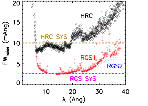
Figure 1: The noise level in terms of the equivalent width of an absorption line for RGS1 (red), RGS2 (blue) and HRC (black). The limits set by the effective area systematics for RGS and HRC are indicated with a purple and brown dashed lines, respectively.

4 Analysis of X–ray lines from the WHIM

4.1 WHIM ions and Galactic lines

In collisional ionization equilibrium (CIE) and for metal abundances proportional to the Solar ratios (e.g. Anders & Grevesse, 1989), the absorption lines with the largest expected equivalent width at a peak temperature $\log T(K)\geq 6$ are the Lyman–$\alpha$ O VIII, He–$\alpha$ O VII, and the Ne IX He–$\alpha$ and Lyman–$\alpha$ Ne X (see Table 3). The ionization curves of key ions of interest to this study are shown in Figure 2 (Mazzotta et al., 1998).

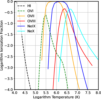
Figure 2: Ionization curves of key ions from Mazzotta et al. (1998).

Of particular interest to the detection of the WHIM in the $\log T(K)=6-7$ temperature range are the O VII and O VIII ions, which are expected to provide the most prominent absorption line features in the XMM-Newton grating spectra. One of the main sources of possible confusion and misidentification for redshifted WHIM lines are absorption lines from lower–ionization X–ray oxygen ions that generate from inner–shell transitions. In recent years there has been significant theoretical and experimental progress in the identification of inner–shell transitions in oxygen ions (e.g. Gatuzz et al., 2015; Gu et al., 2005; García et al., 2005), with some of the strongest relevant absorption lines from inner–shell oxygen ions being reported in Table 3. The net effect of these oxygen–series lines is to make the wavelength range from 21.6 Å (the $z=0$ O VII He-$\alpha$ line) to 23.51 Å (the $z=0$ O I $1s-2p$ line, marking the location of the oxygen edge) effectively unavailable to search for O VII and O VIII absorption lines from the WHIM, given possible velocity structure in the Galaxy, and the resolution of the grating spectrometers.

Table 3: Wavelengths and atomic properties of key WHIM lines, and of inner–shell oxygen Galactic lines that may cause confusion in the identification of redshifted oxygen WHIM lines. References for atomic data: Verner et al. (1996) (V96); Gu et al. (2005) (G05); Gatuzz et al. (2015) (G15); Gharaibeh et al. (2011) and Nicastro (2018) (G11). See also Table 1 of Nevalainen et al. (2017) for other lines of relevance to the WHIM, and García et al. (2005) for other $K\alpha$ atomic data for oxygen.

Ion	Line	Wavelength (Å)	Osc. strength	Reference
WHIM lines
O VII	$1s^{2}-1s2p$ (He$\alpha$)	21.602	0.696	V96
O VII	$1s^{2}-1s3p$(He$\beta$)	18.629	0.146	V96
O VIII	$1s-2p$ (Ly$\alpha$)	18.969 (18.973,18.967)	0.416	V96
O VIII	$1s-3p$ (Ly$\beta$)	16.006 (16.007,16.006)	0.079	V96
Ne IX	$1s^{2}-1s2p$ (He$\alpha$)	13.447	0.724	V96
Ne X	$1s-2p$ (Ly$\alpha$)	12.134 (12.138,12.132)	0.416	V96
Galactic lines
O I	$2p^{4}-[1s]2p^{5}$	23.506	—	G15
O I	$2p^{4}-[1s]2p^{4}3p$	22.889	—	G15
O II	$2p^{3}-[1s]2p^{4}$	23.346	—	G15
O II	$2p^{3}-[1s]2p^{3}3p$	22.287	—	G15
O III	$2p^{2}-[1s]2p^{3}$	23.110, 23.057	—	G15
O IV	$1s^{2}2s^{2}2p-1s2s^{2}2p^{2}$	22.741	0.46	G05
O V	$1s^{2}2s^{2}-1s2s^{2}2p$	22.363	0.55	G05
O VI	$2s^{2}-[1s]2s2p$	22.024	—	G15
N II	$1s^{2}2s^{2}2p^{2}-1s2s^{2}2p^{3}$	29.99-31.16	—	G11

Table 4: List of O VI and H I BLA lines in the FUV spectra of 1ES 1553+113 from Danforth et al. (2016). The numbers identify absorption line systems 1–8

	Redshift	Obs. wavelength $\lambda$ (Å)	Line ID	EW (mÅ)	$b$ (km s-1)	$\log N$ (cm-2)
1	0.187601	1225.52	OVI 1032	64$\pm$5	14.9$\pm$2.5	13.85$\pm$0.09
2	0.187774	1225.69	OVI 1032	65$\pm$8	15.3$\pm$3.5	13.85$\pm$0.11
3	0.189833	1227.82	OVI 1032	37$\pm$37	25.0$\pm$4.9	13.51$\pm$2.18
1	0.187570	1232.24	OVI 1038	24$\pm$5	6.5$\pm$4.0	13.71$\pm$0.08
2	0.187705	1232.38	OVI 1038	50$\pm$6	39.6$\pm$6.5	13.94$\pm$0.06
3	0.189858	1234.62	OVI 1038	10$\pm$3	20.1$\pm$9.9	13.28$\pm$0.22
4	0.394964	1439.52	OVI 1032	69$\pm$7	37.5$\pm$2.6	13.80$\pm$0.04
4	0.394995	1447.46	OVI 1038	64$\pm$12	57.24$\pm$.8	14.04$\pm$0.07
5	0.034656	1257.78	Lya 1215	69$\pm$7	72.0$\pm$9.4	13.12$\pm$0.04
6	0.042726	1267.59	Lya 1215	117$\pm$6	63.0$\pm$4.5	13.38$\pm$0.02
7	0.063637	1293.01	Lya 1215	47$\pm$23	76.3$\pm$19.9	12.96$\pm$0.16
8	0.218690	1481.50	Lya 1215	28$\pm$8	62.6$\pm$21.8	12.72$\pm$0.12

Table 5: Results of the spectral fits to the 1ES1553+113 XMM-Newton data with the spline and slab models.

$z$			$C$ stat.		O vii		O viii		Ne ix		$\Delta C$ (dof)
#	Value	Fixed/Free	Value	d.o.f.	$\log{N}$(cm-2)	$\Delta\ C$	$\log{N}$(cm-2)	$\Delta\ C$	$\log{N}$(cm-2)	$\Delta\ C$
Redshift priors from FUV
1	$0.1876$	Fixed	1861.8	1478	15.13${}^{+0.19}_{-0.31}$	4.2	15.3${}^{+0.3}_{-8.3}$	0.8	15.26${}^{+0.26}_{-0.62}$	1.8	6.8 (3)
2	$0.1878$	Fixed	—
3	$0.1898$	Fixed	1865.8	1478	9.3${}^{+5.3}_{-2.3}$	0.0	15.50${}^{+0.24}_{-0.49}$	2.3	15.26${}^{+0.26}_{-0.66}$	1.7	4.0 (3)
4	$0.3950$	Fixed	1869.6	1478	14.7${}^{+0.4}_{-7.7}$	0.3	14.0${}^{+1.1}_{-7.0}$	0.0	8.0${}^{+6.3}_{-1.0}$	0.0	0 (3)
5	$0.0347$	Fixed	1869.7	1478	14.5${}^{+0.6}_{-7.5}$	0.1	13.6${}^{+1.5}_{-6.6}$	0.1	7.0${}^{+8.0}_{-0.0}$	0.1	0.1 (3)
6	$0.0427$	Fixed	1869.0	1478	14.9${}^{+0.4}_{-7.9}$	0.5	15.0${}^{+0.4}_{-8.0}$	0.8	7.0${}^{+7.4}_{-0.0}$	0.7	0.6 (3)
7	$0.0636$	Fixed	1869.1	1479	—		9.4${}^{+5.7}_{-2.4}$	0.0	15.1${}^{+0.4}_{-8.1}$	0.7	0.7 (2)
8	$0.2186$	Fixed	1867.9	1480	14.97${}^{+0.24}_{-0.57}$	2.0	—		—		—
Redshifts from Nicastro et al. (2018)
9	$0.4336^{+0.0005}_{-0.0003}$	Free	1835.6	1477	15.74$\pm{0.11}$	30.9	14.2${}^{+0.9}_{-7.2}$	0.0	15.30${}^{+0.25}_{-0.38}$	2.6	34.1 (4)
10	$0.3557^{+0.0006}_{-0.0006}$	Free	1864.3	1477	15.29$\pm{0.22}$	4.8	9.9${}^{+5.7}_{-2.9}$	0.0	14.0 ${}^{+0.3}_{-7.0}$	0.7	5.5 (4)

4.2 Models for continuum emission and absorption lines

The analysis of the XMM-Newton spectra was limited to the 13–33 Å range, where all lines of interest from the O VII  O VIII and Ne IX ions are located, at the redshifts provided by the FUV priors. The continuum emission in the 1ES 1553+113 spectra were fit to a cubic spline model (spline in SPEX), given that a simple power–law model across the entire range of interest does not provide a satisfactory fit, due to the relative large count rate of the source. Foreground absorption by the Galaxy was modeled with two hot model components, one for the neutral disk and one for the hot halo, same as in the Ahoranta et al. (2020) investigation of 3C 273, to which the reader is referred for further details.

Possible absorption by the WHIM is modeled with a slab model, which provides the atomic data and the column density of all possible ions of interest, including O VII, O VIII, and Ne IX. This model has the advantage of allowing for all known absorption lines from the chosen ions to be modeled simultaneously. The model does not enforce a specific temperature or method of ionization for the absorbing plasma (as is the case for the hot model), so that all possible absorption line features can be identified and studied. This is the same WHIM absorption model used in previous studies, such as Nevalainen et al. (2017) and Ahoranta et al. (2020).

4.3 Analysis and results for lines with FUV priors

4.3.1 Methods of spectral fitting

A slab WHIM absorption model was used to investigate the presence of absorption lines at the eight redshift systems identified from the FUV data (see Table 4). For each of the 24 redshifted ions identified in the FUV (the 8 systems from Table 4, each with three possible X–ray ions), the spline model was supplemented by one slab model at a time, and the constraints on X-ray absorption for these FUV systems are provided in the top part of Table 5. Redshift systems 1 and 2 are separated in redshift by such a small amount that a redshifted O VII K$\alpha$ lines would be separated by just 4 mÅ, well below the resolution of these data. Therefore we did not repeat the fits for redshift system 2, and the two redshift systems share the same X–ray analysis.

Specifically, we performed 7 different fits, where the same spline continuum model (and the foreground model components) was supplemented by a different slab model in each fit, in which the O VII  O VIII and Ne IX column densities were left free to vary, at a fixed redshift. In so doing, the fit is able to determine whether there is significant absorption from any of the ions under consideration, at that fixed redshift, and from all the ions as a whole. The results of these fits are reported in Table 5, where each line corresponds to each of the seven regressions at a fixed value of the redshifted absorbing material.

The possible O VII at redshift system 6 ($z=0.0427$) falls at a redshifted wavelength of $\lambda=22.524$, which is nearly indistinguishable from the redshifted wavelength of O VIII at redshift system 1-3 ($\lambda=22.528-22.569$), and therefore some of these fits overlap the same wavelengths. For some ions, such as O VII at redshift system 7 and Ne IX at redshift system 8, the main expected absorption lines falls in or near a gap in the data. Accordingly, since these data could not constrain them effectively, the result of the fit was not reported.

4.3.2 Statistical methods for the WHIM absorber component

The main goal of these spectral models is to determine the presence of X–ray absorbing material along the sightline and at a fixed redshift. This, in turn, means determining whether the additional slab component is significant in the fit. To aid with the determination of the significance of detection of a specific ion at a fixed redshift, the $\Delta C=C-C_{\text{min}}$ statistic is also reported in the same table, to represent the increase in the $C$ statistic when the additional slab component is ignored. To measure the $\Delta C$ statistic, we fixed the column density of each of the three ions at the lowest value allowed by the model (which is $\log N(\text{cm}^{-2})=7$, de facto corresponding to zero column density), and repeated the fit in order to calculate the increase in the fit statistic with one fewer model parameter. We also performed an additional fit in which the column density of all three ions were simultaneously frozen to the lowest value, and calculated the overall $\Delta C$ statistic with 3 fewer free parameters. This is the value reported in the rightmost column of the table, along with the number of additional degrees of freedom in the fit. For redshift system 7 and 8, some of the lines were unobservable, thus the number of free parameters in the fit was adjusted accordingly.

The $\Delta C$ statistic is a likelihood–ratio statistic, as described by S.S. Wilks (Wilks, 1938, 1943) and widely used for astronomical statistics (e.g., Cash, 1979; Protassov et al., 2002). Under a number of mathematical conditions described in detail in Cramer (1946), a likelihood–ratio statistic such as $\Delta C$ (but also, for example, the $\Delta\chi^{2}$ or $F$ statistics), is asymptotically distributed like the $\chi^{2}$ distribution, for sources with sufficiently large number of counts (Kaastra, 2017; Bonamente, 2020), as is the case for these data. The number of degrees of freedom of the parent $\chi^{2}$ distribution is determined by the number of free parameters of the additional model component. Since the column density of the ion is the only free parameter in the fit for the $\Delta C$ statistics reported in Table 5 (except those in the last column, where the number of degrees of freedom is reported explicitly), the null hypothesis that there is no absorption from that ion yields a parent distribution for the statistic that is approximately $\Delta C\sim\chi^{2}(1)$, with 90%, 99% and 3–$\sigma$ (99.7%) critical values of respectively $C_{\text{crit}}=2.7,6.6,8.8$.

Before interpreting the results of Table 5, it is necessary to remember that one of the conditions for the use of this likelihood–ratio statistic is that the additional component is nested, i.e., it can be zeroed–out by a suitable choice of the additional parameter(s), corresponding to the null hypothesis that there is no absorbing material. The other main condition is that the value of the parameter(s) that correspond to the null hypothesis is not on the boundary of the allowed parameter space. While the first condition is clearly satisfied, the additional slab model component fails the second condition, in that the absorber can only have a positive column density, i.e., it can only give rise to an absorption line, and not an emission line. This issue is described in detail in Protassov et al. (2002), including an indication that often (but not always or necessarily) using the $\chi^{2}(1)$ distribution as a test for the measured $\Delta C$ leads to a conservative test of the necessity of the component, when the null hypothesis value of the parameter falls at the boundary of the allowed parameter space. This means that, if the measured $\Delta C$ exceeds the critical value of the $\chi^{2}(1)$ distribution, the component should be regarded as significant at that level of confidence, or higher. 

4.3.3 Analysis with a simplified power–law model

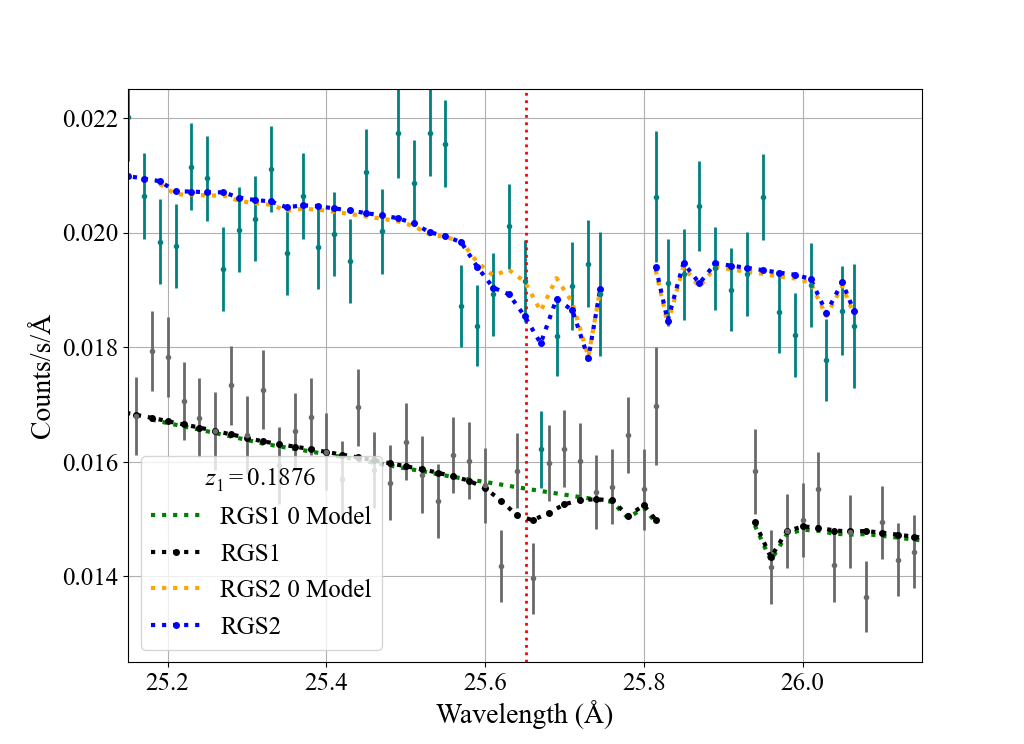
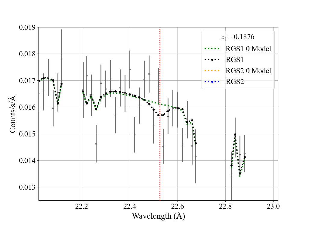
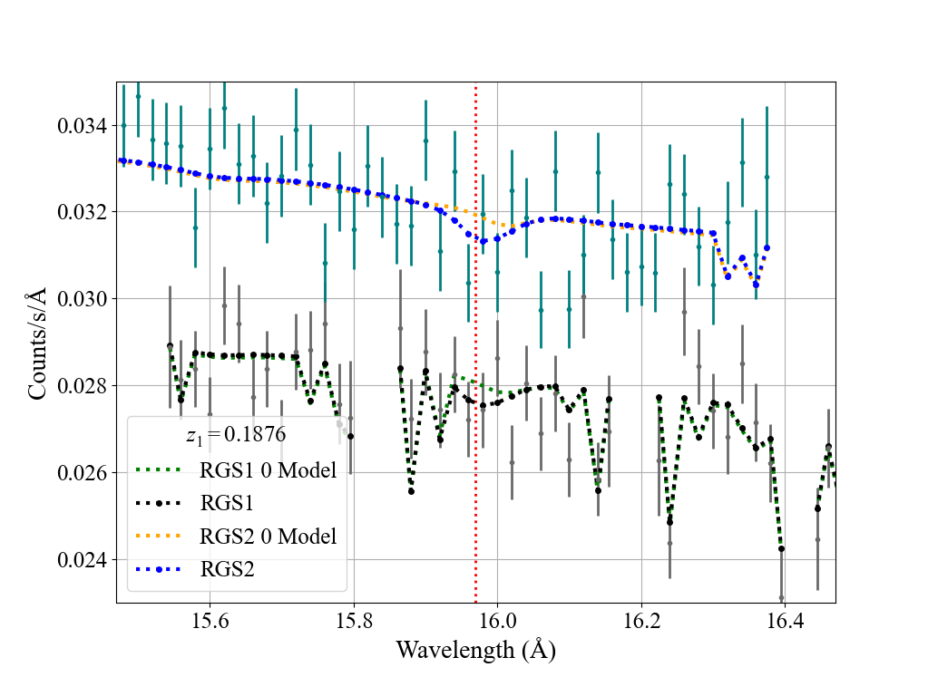
Figure 3: From top to bottom: Portion of the XMM-Newton spectra near the O VII, O VIII and Ne IX at $z=0.1876$. In the top and bottom panels, the RGS2 data (blue) were shifted by a factor of 1.2 for clarity. Vertical lines mark the wavelengths of the redshifted lines.

Given that the requirements for testing the null hypothesis with a likelihood–ratio test are not fully satisfied by the slab model, we also performed additional fits consisting of the use of a simple power–law emission model in a narrow wavelength range, supplemented by a phenomenological line model, which allows for both negative and positive fluxes around the null hypothesis of an optical depth at line center of $\tau_{0}=0$, thus satisfying the criteria for hypothesis testing with a $\chi^{2}$ distribution for the resulting $\Delta C$ statistics. Although this model does not have the convenient features of the slab model (i.e., the atomic physics needed to interpret a fluctuation as an ion column density), this additional regression is more readily capable of answering the question of whether there is a line–like fluctuation in correspondence of the expected X–ray lines. These additional fits were only performed for a few selected lines where the results of Table 5 indicates the possibility of an absorption line feature. They are summarized in Table 6, where the $p$ values correspond to the use of the $\chi^{2}$ distribution for the $\Delta C$ statistics. The line model was used as a Gaussian profile (setting to zero the Lorentzian component), and with a fiducial line width fixed at 10 mÅ, since its use is only to detect the presence of a fluctuation at the target wavelength. Relevant portions of the spectra are shown in Figure 3 for the O VII, O VIII and Ne IX ions at $z=0.1876$ (redshift 1). In Table 6, column densities associated with the line component are estimated via the equivalent width of the line provided by SPEX as part of the fit, and with the assumption of an optically thin line (e.g., using Eq. 2 of Bonamente et al., 2016).

Table 6: Additional fits using a power–law continuum model and a line model. For each regression, a band of 1 Å around the expected line center was used in the fit. For the lines with FUV prior, the line center was fixed. For the other lines from Nicastro et al. (2018), the line center was left free to vary, and the index of the power-law was fixed at a fiducial value. The last two column report the redshift–trial–corrected $P$–values, according to the binomial distribution method, and using a simulation following the Kaastra et al. (2006) method. For the line model, the implied column densities are estimated from the measured equivalent widths, assuming optically thin lines (i.e., Eq. 2 of Bonamente et al. 2016).

Target line	$C_{\text{min}}$	power–law component		line component			$\Delta C$	$p$–value	Corrected $p$–value
	(d.o.f.)	norm.	index	$\lambda$ (Å)	$\tau_{0}$	$\log N(\text{cm}^{-2})$	(d.o.f.)		$P_{\text{binom}}$	$P_{\text{sim}}$
O VII $z=0.1876$ (# 1)	103.5(87)	1968$\pm^{685}_{481}$	0.886$\pm^{0.385}_{0.412}$	25.6545	$0.57\pm^{0.27}_{0.25}$	$15.26\pm^{.14}_{.21}$	6.6(1)	$1.0\times 10^{-2}$	—	—
		1909$\pm^{661}_{463}$
O VIII $z=0.1898$ (#3)	38.4(28)	$760.9\pm^{8.0}_{6.7}$	2.0	22.569	$0.41\pm^{0.45}_{0.31}$	$15.53\pm^{.23}_{.33}$	1.6(1)	0.21	—	—
O VII $z=0.4339$ (free)	119.7(87)	$486.0\pm^{5.2}_{5.4}$	2.5	$30.975\pm^{0.009}_{0.007}$	$3.33\pm^{1.45}_{1.10}$	$15.73\pm^{.13}_{.05}$	29.9(2)	$3.2\times 10^{-7}$	$4\times 10^{-5}$	<0.001
		$476.0\pm^{4.5}_{4.6}$
O VII $z=0.3551$ (free)	117.6(90)	$814.6\pm^{8.6}_{7.2}$	2.0	$29.283\pm^{0.020}_{0.008}$	$0.92\pm^{0.63}_{0.35}$	$15.38\pm^{.22}_{.13}$	8.2(2)	$1.7\times 10^{-2}$	0.88	0.46
		$780\pm^{7.5}_{5.5}$

4.3.4 Results of the analysis

The combination of the results shown in Table 5 and 6 indicates that, of the eight redshift systems with prior FUV absorption detected, there is only evidence for the detection of O VII in redshift system 1 at $z=0.1876$, with a null hypothesis probability of approximately 1%. This null hypothesis probability, if used in a standard normal distribution, corresponds to the probability to exceed $\pm 2.6$ standard deviations (see, e.g., Table A.2 in Bonamente, 2022) and therefore it is equivalent to a 2.6–$\sigma$ level of significance for a possible detection. The significance of detection is obtained from the analysis of the $\Delta C$ statistic for the power–law plus line model, where the conditions for the interpretation of the measured $\Delta C=6.6$ for a nested model component are satisfied. The spline plus slab model analysis (Table 5, $\Delta C=4.2$) cannot be immediately interpreted with a quantitative $p$–value, since the null–hypothesis value of the nested model component (column density $N=0$) is at the boundary of parameter space, as discussed in the previous section.

None of the other O VII, O VIII or Ne IX lines appear to be present in the data. In fact, the second largest $\Delta C$ statistic from Table 5 (for O VIII at redshift system 3) indicates that, upon reanalysis with the power–law plus line model in Table 6, is clearly not significant (null hypothesis probability of 21%). It is also useful to point out that the possible O VII detection has an estimated column density that is just above the $\log N(\text{cm}^{-2})=15.0$ limit associated with the systematic errors discussed in Sect. 3.2.

A list of galaxies along the sightline towards 1ES 1553+113 and in a redshift range of $\pm 0.05$ of the O VI redshift ($z=0.1876$) are reported in Table 7. At that redshift, 1 arcmin separation corresponds to a transverse distance of $\sim 190$ kpc, for a standard WMAP9 $\Lambda$CDM cosmology (Wright, 2006; Hinshaw et al., 2013). The smallest sight–line distance is 5 arcmin, i.e. 1 Mpc, or $\sim 5\times r_{200}$. The EAGLE simulations analysis by Wijers et al. (2020) show that O VII column densities with impact parameters $1-3\times r_{200}$ drop rapidly below $\log N(O~{}VII)=15$ for galaxies of any mass. It is therefore clear that even the galaxy at the closest impact parameter is not sufficiently close to the sightline to be able to cause the tentative O VII absorption line.

Table 7: Galaxies along the sightline towards 1ES 1553+113  at redshifts $z=0.182-0.192$, from the NASA Extragalactic Database.

No.	Object Name	RA (degrees)	DEC (degrees)	Redshift	Magnitude and Filter	Separation (arcmin)
1	WISEA J155552.00+111536.2	238.96668	11.26004	0.18939	19.1g	4.74
2	WISEA J155556.00+111558.8	238.98332	11.26633	0.1875	18.9g	5.57
3	WISEA J155517.24+111307.3	238.82160	11.21872	0.18572	20.7g	6.57
4	WISEA J155521.73+110557.5	238.84056	11.09932	0.18823	19.7g	7.55
5	WISEA J155507.95+111208.2	238.78314	11.20226	0.19089	20.0g	8.64
6	2MASS J15551843+1104530	238.82681	11.08144	0.18777	19.4g	8.89
7	WISEA J155525.65+111955.5	238.85674	11.33199	0.18459	19.7g	9.53

Parameter	Value
	OVII	OVIII
RGS1 Power-laws (continua)
$\alpha_{1}$	1.32${}^{+0.21}_{-0.21}$	4.82${}^{+0.19}_{-0.17}$
Norm1	1435${}^{+235}_{-204}$	145${}^{+16.1}_{-16.0}$
Range (Å)	25-27	22-24
$\alpha_{2}$	1.48${}^{+0.42}_{-0.41}$	1.51${}^{+0.19}_{-0.18}$
Norm2	1032${}^{+276}_{-222}$	1011${}^{+92.0}_{-86.3}$
Range (Å)	21.5-23.1	19.1-20.7
$\alpha_{3}$	1.0 (Fixed)	2.80${}^{+0.61}_{-0.64}$
Norm3	1868${}^{+17}_{-17}$	464${}^{+299}_{-171}$
Range (Å)	29.5-30.5	26-27
RGS2 Power-laws (continua)
$\alpha_{1}$	1.69${}^{+0.19}_{-0.19}$	–
Norm1	1061${}^{+157}_{-138}$	–
Range (Å)	25-27	22-24
$\alpha_{2}$	–	2.11${}^{+0.41}_{-0.44}$
Norm2	–	742${}^{+164}_{-124}$
Range (Å)	21.5-22.8	19.1-20.7
$\alpha_{3}$	0.049${}^{+0.74}_{-1.14}$	1.80${}^{+0.64}_{-0.64}$
Norm3	4241${}^{+6850}_{-2012}$	970${}^{+598}_{-373}$
Range (Å)	29.5-30.5	26-27
Stacked O VII Absorption Line Model
Redshifts	1, 3, 4, 5, 6, 8
Line $\tau_{0}$ (linked)	0.27${}^{+0.13}_{-0.12}$
	(or $\log N_{\text{OVII}}(\text{cm}^{-2})=14.94\pm^{0.18}_{0.22}$)
DOF	325
$C$–stat (expect.)	380.01 (337.11 ${}^{+}_{-}$25.97)
$\Delta C$	5.02
$p$–value	0.025
Stacked O VIII Absorption Line Model
Redshifts	1, 3, 4, 5, 6, 7
Line $\tau_{0}$ (linked)	0.15${}^{+0.082}_{-0.13}$
	(or $\log N_{\text{OVIII}}(\text{cm}^{-2})=15.07\pm^{0.17}_{0.87}$)
DOF	272
$C$–stat (expect.)	323.04 (285.07 ${}^{+}_{-}$23.88)
$\Delta C$	1.57
$p$–value	0.21

Table 8: Spectral fit for the stacked O VII and O VIII WHIM lines. In order to include all possible lines, the RGS data were fit in three narrow–band intervals (i.e., 25-27Å, 21.5–23.1 Å and 29.5–30.5 Å for O VII) with line models at the expected wavelengths for the redshift systems under consideration (e.g., redshift systems 1,3,4,5,6,7 and 8 for O VII). The normalization and optical depth at line center ($\tau_{0}$) for the line models were linked among all the lines. Power–law index $\alpha_{3}$ for the O VII fits was fixed, due to calibration uncertainties in that band.

Table 9: Results of the power–law plus line model for the Chandra LETG data. The $\Delta C$ statistic refers to zeroing out the nested line component. The rightmost column reports the $\Delta C$ statistic corresponding to the comparison between the best–fit model, and a model where the line component was fixed at the XMM-Newton RGS best–fit values from Table 6, instead of the best–fit from Chandra data (this table).

Target line	$C_{\text{min}}$	power–law component		line component				RGS best-fit
	(d.o.f.)	norm.	index	$\lambda$ (Å)	$\tau_{0}$	$\log N(\text{cm}^{-2})$	$\Delta C$	$\Delta C$	d.o.f.
O VII $z=0.1876$ (# 1)	80.66(77)	$1510\pm^{31}_{31}$	2.0	25.6545	$0.32\pm^{0.60}_{0.46}$	$15.03\pm^{0.34}$	0.44	0.2	1
O VIII $z=0.1898$ (#3)	28.82(30)	$1369\pm^{35}_{35}$	2.0	22.5693	$1.37\pm^{2.2}_{1.0}$	$15.87\pm^{0.22}_{0.45}$	2.09	—	—
O VII $z=0.4339$ (free)	92.45(76)	$876\pm^{21}_{20}$	2.5	31.0138	$0.51\pm^{0.7}_{1.0}$	$15.23\pm^{0.31}$	0.77	10.9	2
O VII $z=0.3551$ (free)	97.26(76)	$1426\pm^{33}_{32}$	2.0	29.3492	$2.06\pm^{1.1}_{1.1}$	$15.70\pm^{0.11}_{0.24}$	6.58	5.3	2

Table 10: Selected parameters of the spline model used in the fits of Table 5. Parameter $y001$ refers to the spline component at the lowest wavelength considered $\lambda=13$Å, and $y014$ for that at $\lambda=26$Å .

#	$z$	y001	y014
1	$0.1876$	$990^{+20}_{-21}$	$5178^{+50}_{-45}$
3	$0.1898$	$993^{+20}_{-24}$	$5178^{+49}_{-42}$
4	$0.3950$	$977^{+19}_{-20}$	$5251^{+42}_{-43}$
5	$0.0347$	$970^{+193}_{-135}$	$5182^{+372}_{-401}$
6	$0.0427$	$995^{+20}_{-23}$	$5149^{+51}_{-88}$
7	$0.0636$	$966^{+193}_{-134}$	$5168^{+388}_{-384}$
8	$0.2186$	$994^{+21}_{-24}$	$5143^{+79}_{-64}$
Redshifts from Nicastro et al. (2018)
9	$0.4336^{+0.0005}_{-0.0003}$	$974^{+28}_{-23}$	$5224^{+58}_{-51}$
10	$0.3557^{+0.0006}_{-0.0006}$	$995^{+19}_{-23}$	$5164^{+43}_{-45}$

4.3.5 Additional Stacking of data

Given the limited evidence for the detection of individual absorption lines from a given redshift system, we experimented with stacking the data in order to improve the statistical sensitivity of the data towards the more numerous absorbers expected at the lower column densities. We estimated the statistical sensitivity of the data in terms of column density as follows. We applied the same slab model used for Table 5 to a region near 26 Å where both RGS1 and RGS2 data are present, and away from detector artifacts. We fit the spectrum and use the $\Delta C=2.7$ criterion to identify an upper limit of $\log N_{\mathrm{OVII}}(\text{cm}^{-2})\simeq 15.3$, which corresponds to a 90% upper limit to the non–detection of O VII. When combining or ‘stacking’ $n$ segments of the spectrum at pre–specified wavelengths, the sensitivity of the stacked spectrum is expected to be improved (i.e., the column density that can be probed is reduced) by a factor of approximately $\sqrt{n}$, based on the reduction of the standard deviation of the average signal by the same factor. For $n=7$, the stacked data are therefore expected to reach a sensitivity of approximately $\log N_{\mathrm{OVII}}(\text{cm}^{-2})\simeq 14.9$. This is the level of O VII column density we expect to probe with the stacking of the spectra.

We stacked a $\pm 0.5$  Å portion of the spectra, centered at the target redshifted absorption line, for all redshift FUV priors for the O VII and O VIII ions. To accomplish this, we performed a different spectral fit, compared to the one that resulted in Table 5. This fit consists of using three narrower portions of the RGS1 and RGS2 spectra, each successfully fit with a simple power law, in such a way that the wavelengths of the FUV O VII and O VIII absorption line models (line in SPEX) were all included in these regions. For each of these two fits, the line models were linked to one another, so that there is only one free parameter ($\tau_{0}$) describing the combined optical depth of the lines at the line center. This method was preferred to the one performed, for example, in the stacking analysis of Kovács et al. (2019), where the spectra are first shifted, and then fit to a model that includes an absorption line. The reason for this choice was primarily due to the fact that fitting in observed (i.e., redshifted) wavelength space preserves more accurately the statistical properties of the data, without being affected by the additional processing that results from the blue–shifting to the rest–frame wavelength. Details of these additional spectral fits are reported in Table 8. We decided to not stack the signal at the Ne IX wavelengths in order to focus on the high–temperature oxygen ions alone, given that the only possible detection is from O VII.

The results of these stacked analyses is that there is marginal evidence for the detection of possible O VII absorption at the combined FUV–prior wavelengths, with a null hypothesis probability of 2.5%, or approximately a 2.2–$\sigma$ significance. The stacking permits to reach a lower average column density of $\log N_{\mathrm{OVII}}(\text{cm}^{-2})=14.9\pm 0.2$, which is consistent with the simple $\sqrt{n}$ improvement in the sensitivity discussed at the beginning of the section. This column density from the staked data is consistent with O VII being present only at redshift system 1. While the expected number of absobers per redshift increases by the stacking procedure, the relatively small redshift path renders the detection probabilities small. We will investigate this issue in more detail in a future work with a larger redshift path. The stacked XMM-Newton data do not reveal any evidence for O VIII absorption at the combined FUV–prior wavelengths.

In addition to the spectral fits, and for the purpose of showing a stacked blue–shifted spectrum in the rest frame, we also combined the relevant regions of the spectrum in Figure 4. For this figure, $\pm 0.5$  Å portions of the spectra were blue–shifted to the rest–frame wavelength of interest, and the data and models added together. In addition, the data are represented as their ratio with respect to the best–fit model, in such as way that the orange points are expected to scatter around the 1.0 value of the ratio. To further illustrate the effect of the best–fit line model, this component was zeroed out to calculate the ratio of data–to–model now represented by the blue data points. The blue data points show that, for the O VII stacking, there is a preponderance of points below the 1.0 value around the rest–frame wavelength center of 21.6 Å, indicating a preference for absorption at those wavelengths (although,as discussed earlier, only with limited significance). The black line further reports the difference between the full model and the model with the line component zeroed out, to illustrate the depth of the best–fit absorption line model for the stacked O VII and O VIII lines with FUV priors. This figure is for illustration purposes only, since the fitting was performed in the proper observed wavelength frame, as reported in Table 8.

4.4 Analysis of the two serendipitous Nicastro et al. (2018) lines

In this section we address the Nicastro et al. (2018) report of the serendipituous detection of putative strong He–$\alpha$ O VII absorption at two redshifts with previously unreported FUV absorption lines. For this purpose, we use the same model as for the FUV priors, with an initial value for the redshift at the best–fit values reported by the previous study (respectively, $z=0.4339$ and $z=0.3551$), but with the redshift of the slab model free to adjust itself to the best–fit value. Results of these fits are reported at the bottom of Table 5. We also used the simplified power–law plus line model described in Sect. 4.3 for the two possible O VII lines, so that we can more readily use the corresponding $\Delta C$ values for hypothesis testing. The results of these additional fits are also reported at the bottom of Table 6, where we left the normalizations of the RGS1 and RGS2 data uncoupled to provide more flexibility in the fit. The relevant portions of the XMM-Newton spectra are shown in Fig. 5, with the red dotted line indicating the redshift of the lines that was identified by the Nicastro et al. (2018) analysis.

As discussed in Sect. 2.1, there are uncertainties in our knowledge of the redshift to 1ES 1553+113, with a most likely redshift of $z\simeq 0.433$. If this is correct, then the serendipitous absorber at $z=0.4339$ would be intrinsic to the source, and unlikely to be associated with the WHIM. Nonetheless, we proceed with the study of both of the reported Nicastro et al. (2018) absorbers, assuming their WHIM origin and further using their $z\leq 0.48$ limit on the source’s redshift.

4.4.1 Statistical analysis of the serendipitous detections

In order to evaluate the statistical significance detection of a serendipitous line, i.e., of a line that did not have a predetermined wavelength, it is necessary to account for the number of ‘redshift trials’, or independent opportunities to detect such feature, as originally proposed by Kaastra et al. (2006). A serendipitous or blind search is such that there are multiple opportunities to interpret the deepest fluctuation in the data as a possible absorption line.

A general method to evaluate the probability of occurrence of such fluctuations in a blind search is that of performing a numerical simulation that includes all the relevant parameters of the search, such as the wavelength range spanned, the shape of the line–spread function (LSF), and the resolution of the instrument. Accordingly, we performed a simulation that uses the XMM-Newton LSF model as parameterized by Kaastra et al. (2006), with line center that can vary between $\lambda_{1}=23.5$ Å and $\lambda_{2}=32$ Å. The first wavelength enforces $z\geq 0$ and avoids the 21.6-23.5 Å range possibly contaminated by several O I–O VI Galactic lines, and the second wavelength enforces $z\leq 0.48$, which is the minimum possible redshift for the source reported by Nicastro et al. (2018) although, as remarked in Sect. 2.1, there is now evidence that the redshift of the source may be $z\simeq 0.433$. In addition, and somewhat conservatively, a 25% reduction of this range is assessed in an attempt to correct for several small regions that are unavailable due to detector efficiency and calibration issues (reported, for example, as blank portions in the spectra of Figure 3), resulting in a search over a wavelength range of size $\Delta\lambda=6.4$ Å.

To emulate the blind search method in our numerical simulation, we stepped the possible absorption–line LSF model by a wavelength interval that is smaller than the 20 mÅ data bin (i.e., by 10 mÅ), and identified the distribution of the $\Delta C$ statistic associated with the strongest negative fluctuation during this search, by comparing two fits obtained, respectively, with and without the line component. Since our data are in the large–count limit in each bin, with at least 400 counts per bin, the $\Delta C$ statistic was approximated by the corresponding $\Delta\chi^{2}$ statistic, assuming Gaussian distribution for the counts in each bin. It is important to point out that, as also suggested by Kaastra et al. (2006), the details of the continuum model are not important, since the fit can be performed on the standardized deviations from such best–fit model, where each bin follows a standard Gaussian distribution, under the hypothesis that the data follow the model. The distribution of this maximum $\Delta\chi^{2}$ of the search, which approximates the sought–after distribution of the maximum $\Delta C$, is reported in Figure 6.

The distribution of Figure 6 can be immediately used to identify critical values of the $\Delta C$ statistic, and thus determine whether the measured statistics for a given line is significant or not. The $p$–values associated with this statistic will be referred to as the ‘corrected $P$ value’ in Table 6. According to this analysis, the $z=0.4339$ serendipitous line has a corrected $P$ value that remains comfortably in excess of the 99.9% confidence level, given that the $p=0.999$ critical value of the distribution is estimated at $\sim 20.0$. On the other hand, the putative $z=0.3551$ has a corrected $P$ value of $\sim$0.46, or a 46% probability that the fluctuation is consistent with the noise level. We therefore conclude that this line is very likely a statistical fluctuation in the data. The method is less accurate in the determination of the exact $p$–value of the measured statistic, especially for lines with a large value of $\Delta C$ such as the first of the two Nicastro et al. (2018) lines, since it is difficult to simulate the tail of the distribution accurately.

An alternative and approximate method to determine the $p$–value of the detection statistics is based on the use of the binomial distribution, and it is described in detail in Bonamente (2019). According to this approximate method, the number $N$ of independent opportunities to detect an absorption line is estimated as

$$N=\dfrac{\Delta\lambda}{\sigma_{\lambda}},$$

where the numerator is the effective wavelength range of the search, accounting for unavailable portions of the spectrum, and the denominator is the resolution of the instrument, interpreted as a characteristic wavelength range required to detect a line or to separate one line from a neighboring one. The first number can be be estimated taking into account the parameters of the search, as described earlier, with $\Delta\lambda\simeq 6.4$ Å. The second number can be estimated to be of order $\sigma_{\lambda}\simeq 50$ mA, which is the approximate resolution of the RGS spectrometers; this method is therefore approximate in that it does not account explicitly for the shape of the LSF, but just the approximate resolution. With these numbers, it is possible to estimate that approximately $N\simeq 127$ independent opportunities were available to detect a serendipitous O VII WHIM absorption line in the spectrum of 1ES 1553+113.

The next step is to determine the statistical significance of the detection, indicated by the null hypothesis probability $P$, and its relationship with the single–trial probability indicated with the usual lower–case $p$. The simplest approximation discussed in Bonamente (2019) and also by Nicastro et al. (2013) is

$$P\simeq pN$$

assuming $pN\ll 1$, which is applicable to this case. The corresponding corrected $P$ values are reported in the last column of Table 6. The redshift–trials–corrected null hypothesis probability for the first line is $P=4\times 10^{-5}$, meaning that there is just a 0.004% probability that this is a chance fluctuation. This is consistent with the results based on the simulation of the $\Delta C$ statistic of Fig. 6. It is therefore possible to conclude that there is strong evidence for the serendipitous detection of a genuine absorption line feature in the spectrum of 1ES 1553+113, which corresponds to O VII He-$\alpha$ at $z=0.4339$. When this null hypothesis probability $P$, inclusive of the number of redshift trials, is reported in terms of a two–sided hypothesis testing with the Gaussian distribution, it corresponds to a 4.1-$\sigma$ level detection. This significance of detection is similar to that reported by Nicastro et al. (2018), well in excess of the 3–$\sigma$ threshold even when accounting for all possible redshift trials.

For the other serendipitous O VII line at $z=0.3551$ reported by Nicastro et al. (2018), it is already evident from the larger $p$ value at a fixed redshift (well below the 3–$\sigma$ threshold) and the corrected $P$ value based on the simulation of the $\Delta C$ statistic that there is no significant fluctuation. This is also consistent with the re–analysis by Nicastro (2018), where the author updated the initial significance of detection for this possible line and indicated that there is no significant evidence for an absorption line at that redshift. It is nonetheless instructive to evaluate the overall probability inclusive of redshift trials also for the second putative line, based on the approximate binomial distribution model. In this case, the $P$ value cannot be calculated according to the simple $pN$ approximation, since this product is a large number. Instead, one needs to follow the binomial probabilities (see Eq. 5 of Bonamente 2019), which consists of evaluating the sum

$$P=\sum_{i=1}^{N}\binom{N}{i}p^{i}(1-p)^{N-i}$$

where $p$ is the standard single–trial $p$–value, in this application $p=0.017$. This calculation results in a redshift–trial corrected probability of $P=0.88$, confirming that this is most likely a random fluctuation, and similar to the $P=0.46$ value obtained according to the distribution of Fig. 6.

4.4.2 Other considerations for these serendipitous features

Having established that the first of the two Nicastro et al. (2018) features is consistent with O VII He–$\alpha$ absorption at $z=0.4339$, it is necessary to discuss its identification. In the absence of a more significant FUV counterpart at the same redshift, the identification with O VII He–$\alpha$ should be regarded as indeed plausible, but only tentative. The accompanying He–$\beta$ would fall near a wavelength of 26.71 Å, but its lower oscillator strength (see Table 3) makes the line less readily detectable. Nicastro et al. (2018), in fact, does not report a statistically significant detection at those wavelengths. There is also the possibility of a misidentification with other Galactic or intervening lines. One such possibility is Galactic N II K–$\alpha$ absorption, which is expected to be present at the same wavelengths as the detected feature, and may in fact be responsible for a portion of the detected absorption (as already discussed in Nicastro, 2018).

Moreover, Johnson et al. (2019) showed that 1ES 1553+113 is likely a member of a group of galaxies located near $z=0.433$, although its redshift could not be measured due to the lack of emission lines in its optical spectrum. The possible location of the source at the same redshift as the putative O VII absorption lines results in the possibility that the feature could be intrinsic to the source itself, also also discussed in Nicastro et al. (2018), or that the absorption is associated with the local intra–group medium, rather than the truly inter–galactic WHIM. It goes beyond the scope of this paper to investigate in more detail the identification of this serendipitous feature. In the following, we will assume that it is entirely due to O VII He–$\alpha$ absorption from the WHIM at $z=0.4339$, as in the original Nicastro et al. (2018) paper, and simply caution the reader that this identification is not confirmed, and it needs to be regarded as tentative.

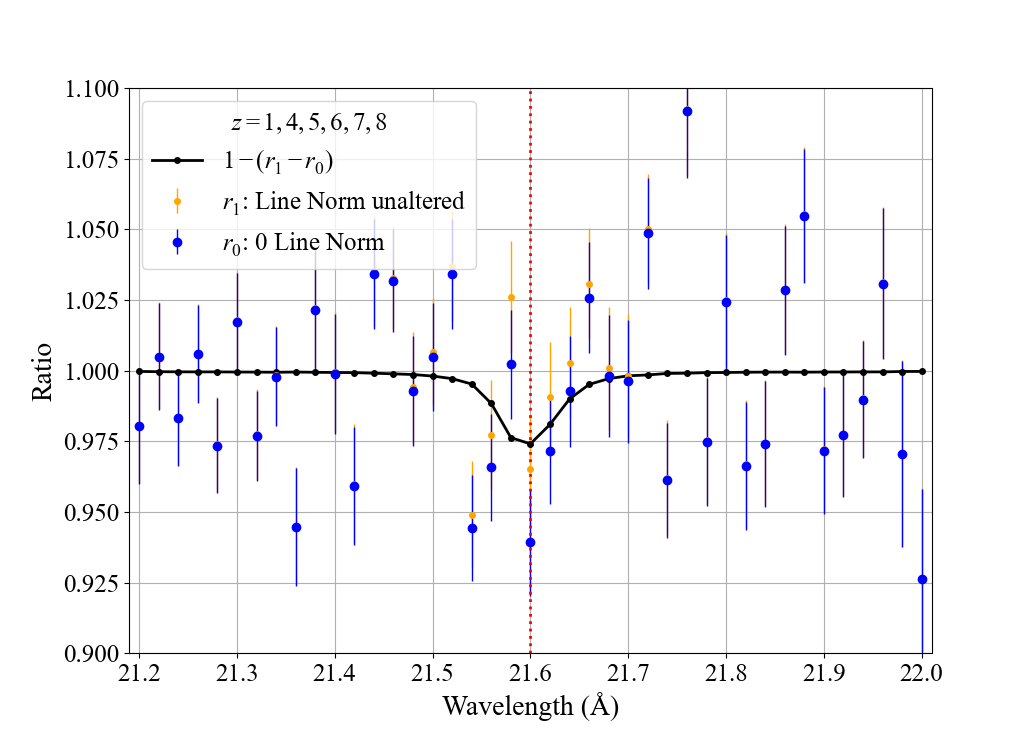
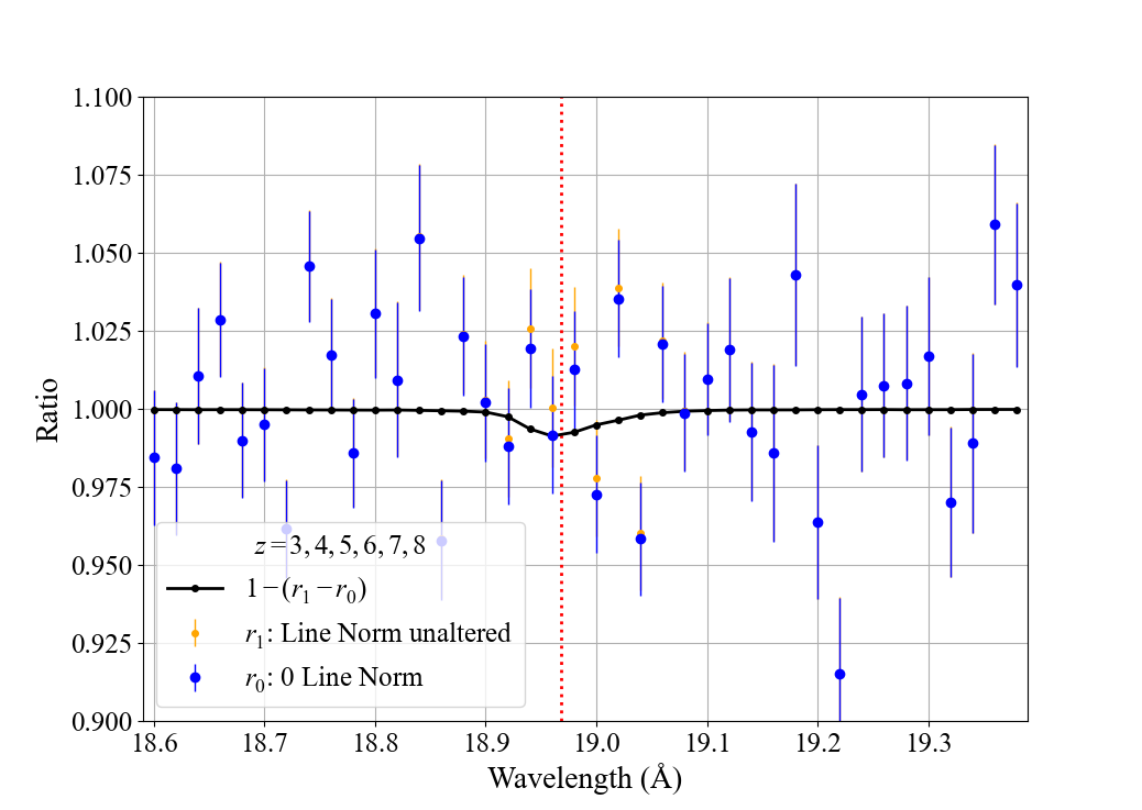
Figure 4: (Left) Stacked spectrum for all O VII lines with FUV priors. The orange data points are the ratio of the stacked data to the model, and the blue data points are the ratio when the OVII line model is zeroed out, to highlight any deficit of counts near the expected line wavelength. In black is the difference between these two ratios. (Right) Same spectrum, but for O VIII lines with FUV priors. The vertical lines mark the rest wavelength of the lines.

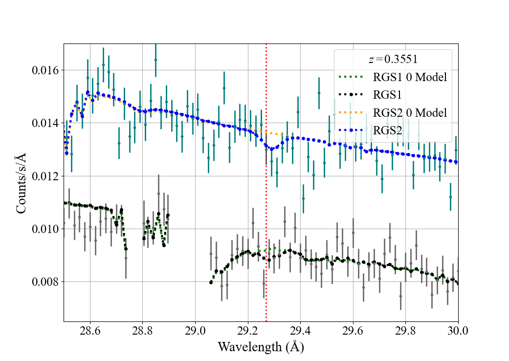
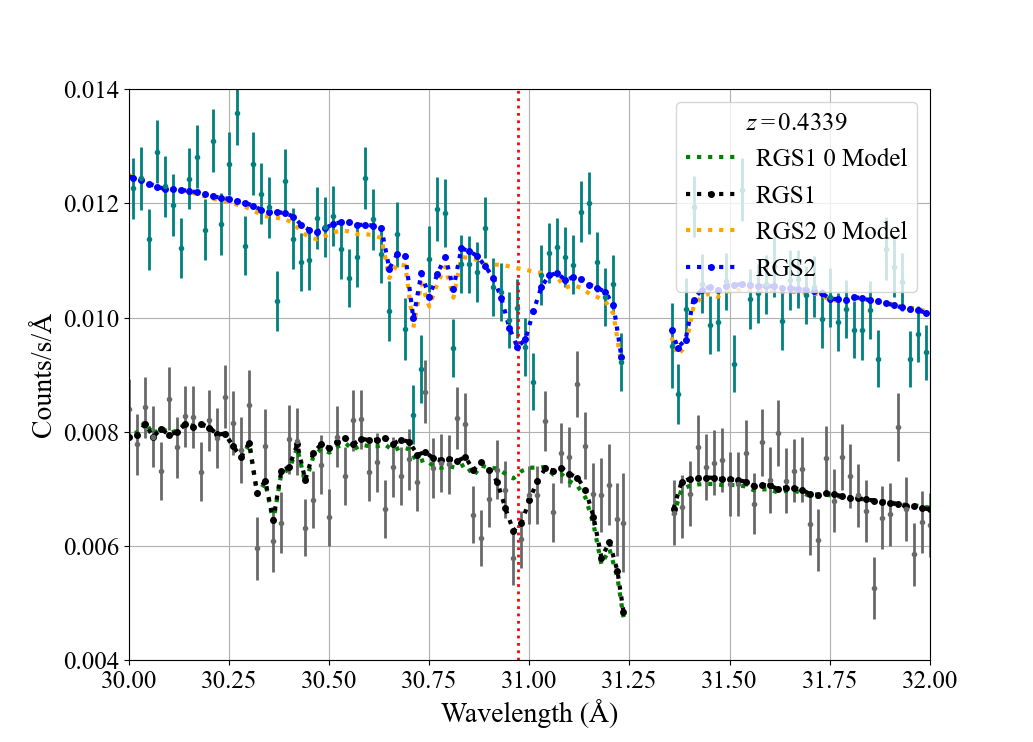
Figure 5: (Left) O VII at $z=0.355$ and (Right:) O VII at $z=0.4339$, at the redshifts identified in the blind search of Nicastro et al. (2018). Gray/black points represent RGS1, and teal/blue represent RGS2 (shifted for clarity by a factor of 1.35). Vertical lines are the wavelengths of the Nicastro et al. (2018) detections.

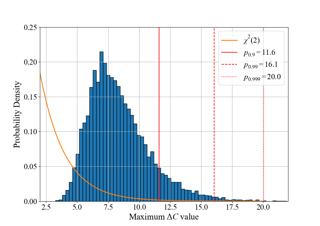
Figure 6: Sampling distribution of the $\Delta C$ statistic for the blind search of an absorption lines, under the null hypothesis that there are no absorption lines, following the method of Kaastra et al. (2006). For comparison it is also plotted the $\chi^{2}(2)$ distribution, which applies to the detection of an absorption line model with two free parameters, but without accounting for redshift trials.

4.5 Comparison of XMM-Newton results with the Chandra data

Despite the lower resolution, it is nonetheless useful to determine whether the Chandra spectra are consistent with the results from the XMM-Newton spectra. The Chandra HRC spectra near the wavelengths of the putative $z=0.1876$ O VII absorption, and for the two Nicastro et al. (2018) lines, are shown in Fig. 7. For each of the spectra, we fit a simple power–law model with a line component, same as in the XMM-Newton fits of Table 6. To compare the results between the two instrument, in one of the fits the parameter(s) of the line–model component were left free, and in the second fit they were fixed at the best–fit parameters from the XMM-Newton regressions. Table 9 shows the results for these fits, including the $\Delta C$ statistic for the comparison between the free–parameter fits, and the fits with the line component fixed at the XMM-Newton value.

The best–fit model for the line component shows that none of the three lines is detected significantly, as can be seen from Fig. 7. In particular, the putative serendipitous O VII $z=0.4339$ line is not detected at all in Chandra at the wavelength and optical depth expected based on the XMM-Newton spectra, despite its strong XMM-Newton detection. To determine the agreement between the two spectra for that line, we determine that the fixed XMM-Newton model corresponds to a $\Delta C=10.8$ statistic (rightmost column in Table 9), compared to the best–fit model based on the Chandra data. Given that the parent distribution of the $\Delta C$ statistic under the null hypothesis that the best–fit XMM-Newton model is correct is a $\chi^{2}(2)$ distribution, the null hypothesis can be discarded at a $\geq 99.9$% confidence level (i.e., the 99.9% critical value is 9.2). This statistic, however, does not mean that there is no absorption line at that redshift – it simply means that the Chandra data suggests a lower parent value than the best–fit XMM-Newton measurement. In practice, this can be interpreted with the fact that the low signal–to–noise of the Chandra data cannot conclusively confirm the XMM-Newton detection, neither completely rule out the absence of the line.

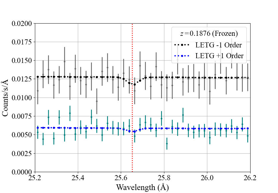
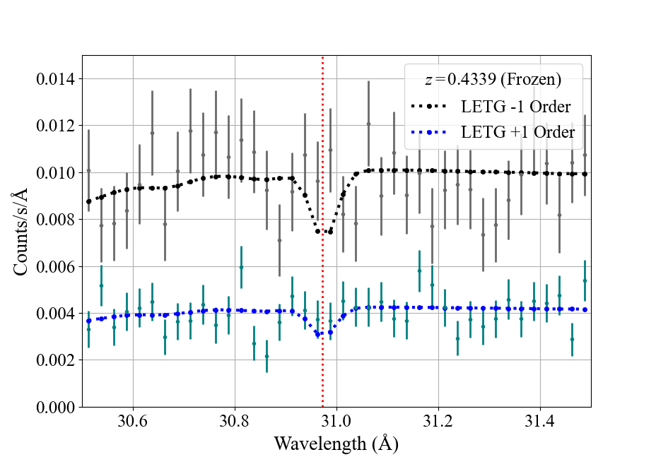
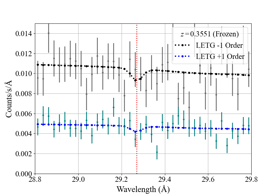
Figure 7: Chandra HRC LETG spectra in 1 Å intervals around the three wavelengths of interest. The -1 order spectra were rescaled by a factor of two, for clarity.

4.6 Sources of systematic uncertainty

The results of the broad–band fits provided in Table 5 show a $C_{\text{min}}$ statistics that consistently exceeds the number of degrees of freedom, i.e., its expectation under the null hypothesis. The typical number of counts per 20 mÅ bin is always larger than $\sim$300 counts across the entire 13-33Å wavelength range, and therefore the $C_{\text{min}}$ statistic is expected to be approximately distributed like a $\chi^{2}$ distribution. This asymptotic distribution is discussed in detail in Kaastra (2017) and in Bonamente (2020, 2022), including in the low–count case. In the case of the redshift system 9, corresponding to the first of the two Nicastro et al. (2018) lines, a $\chi^{2}(1477)$ distribution has an expected value and a standard deviation corresponding to a range $1477\pm 54$, with a one–sided 99.9% critical value of 1651. Given that the measured best–fit statistic exceeds the critical value, even the rather flexible spline continuum model appears insufficient to provide a statistically acceptable fit. The flexibility of the spline model is provided by the large number of parameters used (twenty–one, in 1 Å intervals between 13 and 33 Å), two of which are reported in in Table 10 to illustrate typical uncertainties. Moreover, the two hot components that model the Galactic foregrounds provide a typical reduction in the best–fit by $\Delta C\simeq 50$ for three additional free parameters.

This mismatch between the data and the model can be interpreted either as an indication that the model should be rejected, or that there are other sources of systematic uncertainty that have not been included in the analysis. Given that the data are known to feature possible sources of systematic error, as indicated in Sect. 3, and that the best–fit model generally follows the data well without broad–band systematic deviations, it is reasonable to attribute the slightly higher–than–expected fit statistic with the presence of systematic sources of error that go above the Poisson counting errors.

In the case of regression with Gaussian data, it is possible to account for systematic errors in a number of ways, which typically result in an increase of the uncertainties above the Poisson or $\sqrt{n}$ errors.  For a regression with the Poisson–based $C$ statistic, those avenues are not available, given that the Poisson distribution enforces a variance that is always equal to its mean — in other words, the Poisson distribution does not have the flexibility to change its variance independently of its mean. An alternative method to address sources of systematic error which is applicable to Poisson data consists of considering an intrinsic model variance, whereby the additional source of uncertainty is attributed to the model, and not the data. A method to estimate the intrinsic model variability for Poisson data is presented in a companion paper, where the statistical details of the method are described in detail (Bonamente, 2023). For the present paper, it is sufficient to report that these XMM-Newton data are consistent with a systematic error of order few percent, meaning that the model is subject to variation of this order in each independent bin. This is consistent with the estimate of a few percent systematic error that was briefly discussed in Sect. 3, based on the knowledge of the instruments. Further details on the method to estimate systematic errors can be found in Bonamente (2023).

Fortunately, the narrow–band regressions provided in Table 6 feature fit statistics that are in better agreement with the parent distribution. For example, the value of $C_{\text{min}}=119.7$ for 87 degrees of freedom, corresponding to the fit for the first Nicastro et al. (2018) line at $z=0.4339$, has a 99.9% critical value of 133.5 according to the corresponding $\chi^{2}$ distribution. This makes the measured value of the fit statistic statistically consistent, at that level of confidence, with the model. Similar considerations apply for all the other fits presented in Table 6. Given that the conclusions presented in this paper are based primarily on the results presented in that table, we do not expect that any possible sources of additional systematic errors would have a significant impact on the results of this paper.

5 Cosmological implications of the search for X–ray absorption lines

Of the 8 absorption lines systems detected by Danforth et al. (2016) and used as sign–posts for possible X–ray absorption, there is only marginal evidence for one new detection of O VII (at redshift systems 1 and 2). Given that the search was conducted using an FUV prior for the redshift, the statistical significance of detection is the formal significance as obtained from the detection statistics, without the need to account for redshift trials (which are needed for blind searches, see e.g. Nicastro et al. 2005, 2013; Bonamente 2019). For the other redshift systems, we only obtained upper limits to the non detection of the O VII, O VIII and Ne IX ions.

This section presents the methods to measure the cosmological density of the X–ray absorbing WHIM, and it includes a new statistical framework to account for the limited sensitivity of the X–ray data, the use of FUV priors, and the presence of upper limits. This new method is then applied to the possible detection of O VII at $z=0.1876$ and alternatively to the upper limits to the non–detections for the seven FUV–prior redshifts. The result of this analysis is an estimate of the cosmological density of WHIM associated with the detection or the non–detection of these absorption line systems. It is first necessary to describe the statistical methods used to derive the cosmological constraints, given the unique challenges posed by the low–resolution X–ray data and the selection of the redshifts used to search for X–ray absorption lines.

5.1 Statistical methods to constrain $\Omega_{\mathrm{WHIM,X}}$

The general method to constrain the cosmological density of baryons traced by a specific ion was developed by Tilton et al. (2012) and Danforth et al. (2016), whereby the distribution of the number of absorbers per unit column density and redshift,

$$f(n)=\partial^{2}n/\partial N\partial z,$$ (1)

is used to evaluate the cosmological density

$$\Omega_{\mathrm{ion}}=\dfrac{\rho_{\mathrm{ion}}}{\rho_{c}}=\dfrac{m_{\mathrm{ion}}H_{0}}{\rho_{c}c}\int f(n)NdN$$ (2)

where $N$ is the ion column density and $\rho_{c}$ the critical density of baryons. Given that the bulk of the baryons are expected to be in the neutral and ionized hydrogen, the ion is then used as a tracer of the total baryonic matter via

$$\Omega_{\mathrm{WHIM,ion}}=\Omega_{\mathrm{ion}}\dfrac{\mu_{H}\,m_{H}}{m_{\mathrm{ion}}}\dfrac{1}{A\cdot f_{\mathrm{ion}}(T)}$$ (3)

with knowledge of the chemical abundance $A$ and temperature of the WHIM plasma. The mean atomic mass $\mu_{H}$ represents the mass associated with one hydrogen atom, which is a function of the state of ionization and chemical abundance of the absorber. For a significantly sub–Solar chemical composition, we approximate it with $\mu_{H}=1.3$, similar to what is assumed for other WHIM studies (e.g.. Nicastro et al., 2018). Equation 3 is complicated by the fact that usually neither the chemical abundance or the temperature are known accurately. To overcome these limitations, Tilton et al. (2012) assumed a temperature that corresponds to the peak of the ionization curve for the ion under consideration, and a fixed value of $A=0.1$ Solar, while Danforth et al. (2016) adopted an abundance that was motivated by simulations.

X–ray observations of the WHIM in absorption often yield only a few positive detections, and more often just upper limits to the non-detection of a specific ion. Therefore, it is necessary to investigate an alternative way of constraining the cosmological density of baryons, given that the distribution (1) cannot be constrained effectively with only a few systems available. A useful starting point is the simplification of Eq. 3

$$\Omega_{\mathrm{WHIM,X}}=\dfrac{\mu\,m_{H}}{\rho_{c}}\dfrac{{\sum_{i}}N_{H,i}}{\sum_{i}D_{i}}$$ (4)

(see, e.g., Schaye, 2001; Nicastro et al., 2018) where the sum extends over all available sources, and the $i$–th source probes a cosmological distance $D_{i}$ with a detection of a total WHIM column density $N_{H,i}$, representing the entire baryonic content of the WHIM. It remains to be established how many X-ray absorbers, or how long a path length one needs to probe, so that one can derive reliable estimates for the cosmic baryon budget that are applicable to the entire Universe. Obviously, measurements from one absorber alone, as in the case of these data and those of Nicastro et al. (2018), is not adequate to make cosmological inferences. It is nonetheless useful to develop this method, also for the sake of its applicability to future studies with a larger sample of sources.

When the estimate is provided by a single ion, e.g., O VII or O VIII as is often the case with X–ray observations, equation (4) is equivalent to

$$\begin{cases}\Omega_{\mathrm{WHIM,ion}}=\Omega_{\text{ion}}\dfrac{\mu\,m_{H}}{m_{\mathrm{ion}}}\dfrac{1}{A\cdot f_{\mathrm{ion}}(T)}\text{, with}\\[10.0pt] \Omega_{\text{ion}}=\dfrac{\rho_{\text{ion}}}{\rho_{c}}\text{, and}\\[10.0pt] \rho_{\mathrm{ion}}=m_{\mathrm{ion}}\dfrac{N_{\mathrm{ion}}}{D_{i}},\end{cases}$$ (5)

where $N_{\text{ion}}$ is the column density of the specific ion under consideration and $\rho_{c}$ is the critical density of baryons at the present epoch. In these equation, the temperature and abundance is needed to convert the ion’s column density to the total plasma column density. In principle, temperature constraints can be obtained in the presence of at least two lines from different ions of the same element, such as O VI and O VII (using, e.g., the ionization equilibrium curves of Fig. 2), and the abundances can be also constrained with additional lines from other elements. Such constraints are typically beyond the quality of the current X–ray data, and therefore it is customary to parameterize the resulting cosmological densities in terms of the unknown temperature (or ion fractions) and abundances.

5.2 Using EAGLE to correct for sample selection and X–ray sensitivity limits

The equations developed in the previous section need to be further developed to account for (a) the limited sensitivity of X–ray observations that render a fraction of the WHIM unobservable, (b) the selection of sightlines based on their FUV priors, and also (c) the presence of upper limits to the non–detection. This section provides quantitative methods to address these issues.

5.2.1 Definition of probabilities

The sensitivity of the X–ray observations can be defined as an upper limit, e.g. $N_{\mathrm{OVII}}^{+}$ , with the meaning that the data at hand can only detect a column density of O VII at that redshift than this larger than value, at a given level of confidence. Similar considerations apply also to the other ions. In other words, the available data are not sensitive to column densities $N_{\mathrm{OVII}}$$\leq$$N_{\mathrm{OVII}}^{+}$, due to the limitations of the instrument and exposure times. In order to estimate the fraction of an ion’s column density that in unobservable because of the limited quality of the data, we make use of the EAGLE simulations (Schaye et al., 2015; The EAGLE team, 2017), leveraging the prior relevant analysis by Wijers et al. (2019). Figure 8, reproduced from Wijers et al. (2019), illustrates the EAGLE prediction for the distribution of the column densities of O VI and O VII ions in a $100^{3}$ Mpc³ simulation of the Universe at low redshift, and for the distribution of H I and O VII. These joint distributions are the basis for the prediction of the amount of O VII present along the sightline. The same analysis could be repeated for O VIII, or other X–ray ions. For these ions, there is no information on line widths that was used for their selection, and therefore they represent the entire ionic budget in the EAGLE simulations. The distributions of temperature and abundances of the gas used for Figure 8 are described in detail in Wijers et al. (2019). At $\log N_{\text{OVII}}(\text{cm}^{-2})>15$, the temperature of the gas is primarily in the range $\log T(\text{K})=5.5-6.5$, while at $\log N_{\text{OVII}}(\text{cm}^{-2})>16$ the temperatures are typically $\log T(\text{K})=6.0-6.5$. The metallicity of the absorbers is almost entirely in the range $\log A=-1$ to $-0.5$ Solar.

We start by defining the probability $p_{j}$ that a sightline with a detected O VI column density $N_{\text{OVI}}$ at a specific redshift $z_{j}$ has an amount of O VII larger than the upper limit,

$$p_{j}=P(N_{\mathrm{OVII}}>N_{\mathrm{OVII}}^{+}|N_{\mathrm{OVI}}).$$ (6)

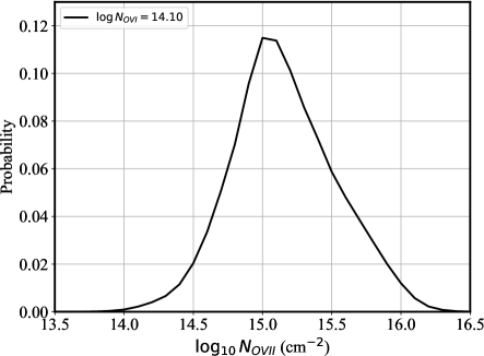
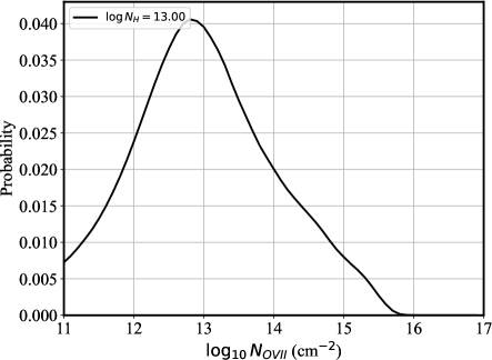
Figure 9: Conditional probability distribution of (a) O VII given a range of O VI, and (b) O VII  given H I, from Wijers et al. (2019). The distributions correspond to the solid red lines in Fig. 8, and have been normalized to a total probability of one.

Such probability distribution is illustrated in Figure 9, which is obtained from a vertical slice of Fig. 8 at a given value of the O VI column density. Same considerations apply to H I, whereby the probability in (6) is obtained by conditioning on the column density $N_{\text{HI}}$ instead of $N_{\mathrm{OVI}}$. Equation 6 reads as the probability that the column density exceeds the upper limit, given the value of the detected O VI column density. Given that the systems under consideration are those with a known value of the O VI and H I column density, the conditional probabilities of (6) illustrated in Fig. 9 can be immediately used to evaluate the probability $p_{j}$ by evaluating the integrated probability above the upper limit. This probability quantifies what $p_{j}<1$ fraction of O VII absorbers, by number, is observable because of the limits in sensitivity of the X–ray data. Usually this value is small, indicating that the data can only detect a small fraction of possible EAGLE–predicted O VII absorbers.

Since the only detectable absorbers (in the CGM and in filaments alike) are the ones with the highest column density, it is necessary to evaluate another probability that describes the fraction of the O VII column density detectable above the upper limit. This probability is defined as

$$P_{j}=\dfrac{\int_{N_{\mathrm{OVII}}^{+}}^{\infty}P(N_{\mathrm{OVII}}/N_{\mathrm{OVI}})dN_{\mathrm{OVII}}}{\int_{0}^{\infty}P(N_{\mathrm{OVII}}/N_{\mathrm{OVI}})dN_{\mathrm{OVII}}}$$ (7)

where $P(N_{\mathrm{OVII}}/N_{\mathrm{OVI}})$ is the same conditional probability distribution used in (6), and it is weighed by the ion column density $dN_{\mathrm{OVII}}$. This probability describes the cumulative fraction of O VII column density that is detectable, and it is a larger number than $p_{j}$ because the larger column densities are the observable ones. The evaluation of $P_{j}$ is illustrated in Fig. 10, where the solid black curve is the cumulative distribution of the marginal probability distribution in Fig. 9, and the blue curve represents the fraction of O VII column density present below that value of $\log N_{\mathrm{OVII}}$, i.e., its cumulative distribution function. For example, for $\log N_{\mathrm{OVII}}^{+}=15.3$, the curve in the left panel shows $p_{j}\simeq 0.36$, corresponding to a fraction $P_{j}\simeq 0.72$ of O VII above that limit. For the same source, these probabilities $P_{j}$ will in general vary with the redshift of the O VI priors, although variations are not expected to be large if the X–ray data have a similar S/N throughout their redshift coverage, as is the case for our data (see Table 5).

In summary, the correction provided by $P_{j}$ according to (7) probability follows the assumption that O VII absorbers are associated with O VI  (or H I), and therefore we use the measured O VI (or H I) column density to estimate the fraction of column density that is missed because of the limited X–ray resolution. A similar analysis can be performed using different simulations, in order to address the dependence of the results on the assumed distribution of the absorbing gas. While an in–depth comparison of these distributions among various simulations goes beyond the scope of this paper, we point out that the CAMELS cosmological simulations (Butler Contreras et al., 2023) feature a similar distribution of O VII vs. H I column densities (see their Figure 4) to the one from EAGLE used in this paper. In general, however, the distribution of column densities of ions are quite sensitive to the choice of simulation methods.

5.2.2 Use of probabilities for cosmological estimates

These probabilities can be now used as follows for obtaining cosmological constraints from the measured column densities.

(1) For a source (labeled by the index $i$) with one or more detections (labeled by $j$), the cosmological density can be constrained to

$$\rho_{\mathrm{ion,i}}=m_{\mathrm{ion}}\dfrac{\sum_{j}N_{\mathrm{ion,j}}/P_{j}}{D_{i}}\simeq m_{\mathrm{ion}}\dfrac{\sum_{j}N_{\mathrm{ion,j}}}{D_{i}\cdot\overline{P_{j}}}$$ (8)

where the sum extends to the number of redshifts with detections (for 1ES 1553+113, this is only one, the putative detection of O VII at redshift system 1) and, in the limit of small differences in the values of the $P_{j}$’s for that ion, the approximation holds with better accuracy when the average value $\overline{P_{j}}$ is used. The effect of $P_{j}$ is to reduce the redshift path or, equivalently, the distance $D_{i}$ probed, to account for the fact that a fraction $(1-P_{j})$ of the total predicted O VII column density was unobservable to begin with. The effect is therefore to boost the cosmological density associated with the actual detection, to recognize the inherent difficulty to achieve the detection that was posed by the limited sensitivity of the data.

(2) In the case of systematic non–detections of an ion (i.e., O VII) at all redshifts, the procedure must account for all upper limits set along each sightline. In fact, the search for the WHIM was conducted at a number of redshifts $z_{j}$ with $j=1,\dots,N_{i}$. In the case of 1ES 1553+113, $N_{i}=7$ independent redshifts were being tried. For each of these redshift trials, EAGLE predicts a distribution of X–ray column densities according to a curve of the type of Figure 9, based on the positive detection of an FUV ion (either O VI or H I). Such systematic non–detection of X–ray absorption can be taken to mean that none of the observable WHIM was present at any redshift where EAGLE predicted it. This situation can be quantified in the following manner.

First we calculate the expectation of the undetectable $N_{\mathrm{ion,j}}$ as

$$\mathrm{E}[N_{\mathrm{ion,j}}^{+}]=\dfrac{\int_{0}^{N_{\mathrm{ion,j}}^{+}}N_{\mathrm{ion}}P(N_{\mathrm{ion}})dN_{\mathrm{ion}}}{\int_{0}^{N_{\mathrm{ion,j}}^{+}}P(N_{\mathrm{ion}})dN_{\mathrm{ion}}},$$ (9)

which is a probabilistic expectation or average column density of what XMM could have missed at that redshift, given the presence of an FUV ion. In this equation, $P(N_{\mathrm{ion}})$ is the same distribution used in (6), but the conditioning on the FUV ion was omitted for the sake of clarity. In other words, this is the average value of the column density of an X–ray ion as predicted by EAGLE for that redshift trial, but that are not detectable due to the sensititivity of the X–ray data; the denominator ensures that the probability distribution is properly normalized.

Such average values can be summed over all non–detections, so that

$$\mathrm{E}[N_{\mathrm{ion}}^{+}]=\sum_{j=1}^{N_{i}}\mathrm{E}[N_{\mathrm{ion,j}}^{+}]$$ (10)

represents an average upper limit to the column density of the ion that was systematically not detected. The use of (10) to estimate the overall upper limit to a systematic non–detection has two main advantages. First, it accounts for all redshift trials; and second, it makes use of both the X–ray sensitivity limits and the expected distribution of X–ray ions according to EAGLE.

This average upper limit can then be used in

$$\rho_{\mathrm{ion}}\leq m_{O}\dfrac{\mathrm{E}[N_{\mathrm{ion}}^{+}]}{D_{i}}$$ (11)

to provide an upper limit to the volume density of the ion, in a manner similar to (8) in the case of a detection. Accordingly, an upper limit to the associated cosmological baryon density of the WHIM is obtained via (5), which requires assumptions on the temperature/ionization fraction, and overall abundance of the element under consideration (i.e., typically oxygen).

It is worth pointing out that, when a sightline such as 1ES 1553+113 has several undetected X–ray lines, $\mathrm{E}[N_{\mathrm{ion}}^{+}]$ is the sum of several terms that increase the average upper limit, above that of a single upper limit. This is reasonable, in that each independent redshift trial represents an independent opportunity, according to the EAGLE predictions, for the presence of associated X–ray ions. An alternative to (10) would be to simply use the least–stringent X–ray upper limit $N_{\mathrm{ion,j}}^{+}$ in place of $\mathrm{E}[N_{\mathrm{ion}}^{+}]$, but such procedure would not account for all redshift trials included in the distance $D_{i}$ probed by the X–ray data.

5.3 Cosmological constraints from 1ES 1553+113

We now illustrate the method provided in the previous section with the column densities measured from the 1ES 1553+113 XMM-Newton data. We entertain two scenarios. First, assuming that the O VII line associated with the $z=0.1876$ absorber is a real astrophysical signal, despite its limited significance of detection, we use (5) to estimate the cosmological significance of the putative detection. Then, we use a more conservative approach to estimate an upper limit to the systematic non–detection of X–ray ions, according to (11). We use a value for the sensitivity of the XMM-Newton spectra to the detection of the O VII ion as $\log N_{\mathrm{OVII}}^{+}\simeq 15.3$, as discussed in Sect. 4.3.5.

For the $z=0.1876$ absorber, we consider an associated O VI column density that corresponds to the sum of the first two FUV lines in Table 4. In fact, these two FUV lines are indistinguishable at the resolution of these XMM-Newton data, and the resolution of the EAGLE distributions (see Fig. 8) is such that those two absorbers would have been counted as one (Wijers et al., 2019). The sensitivity of the X–ray data at hand corresponds to the ability of observing a fraction $P_{j}\simeq 0.72$ of all the available O VII along the sightline, give the presence of $\log N(\text{O~{}VI})\geq 14.1$ at that redshift, according to (7).

5.3.1 The effective redshift path probed

The uncertainties regarding the redshift of 1ES 1553+113 discussed in Sect. 2.1 must be reflected in the cosmological constraints from the FUV–prior search for X–ray absorption lines that we have conducted. The most likely redshift for the source is $z\simeq 0.433$, with an upper limits of approximately $z\leq 0.48$ (Nicastro et al., 2018). Moreover, our choice of the redshift systems to investigate (see Table 4) is limited by the selection effects of the Danforth et al. (2016) study, including the completeness of the H I and O VI systems (see Table 4 in Danforth et al. 2016). Given these uncertainties, we conservatively assume a maximum redshift path of $z\leq 0.48$ for our search of X–ray absorption lines associated with the WHIM. If the $z\simeq 0.433$ is correct, then our estimates of the cosmological density of baryons associated with the lines will be strict lower limits.

Moreover, the redshift path probed by the XMM-Newton data is smaller than the entire $z\leq 0.48$ path up to the maximum estimated redshift of the source. Specifically, several Galactic oxygen lines (at $21.6-23.5$Å, see Table 3) prevent an accurate blind search for O VII at $z\leq 0.09$, and several regions with poor calibration result in an estimated $\sim 25$% reduction in the redshift path probed, as discussed in Sec. 4.4.1. The effective distance probed $D_{i}$ in (5) must therefore be evaluated accordingly. For a flat $\Lambda$CDM cosmology with a dimensionless Hubble constant of $h=0.7$ and a critical matter density at the present epoch of $\Omega_{m}=0.3$, the angular diameter distance to $z=0.48$ is $D_{A}=1.23$ Gpc. The purpose of the ratio $N_{\text{ion}}/D_{i}$ in (5), however, is that of estimating a baryonic density associated with the measured column density. The measured column density $N_{\text{ion}}$ is independent of the cosmology used, since it is the result of the slab model applied to the spectrum, with no explicit dependence on the parameters of the cosmological model. It therefore appears appropriate to estimate the effective distance $D_{i}$ via the comoving distance, which is a function of the comoving volume $V_{C}(z)$ associated with the redshift path available for the search, instead of the angular diameter distance. In this case, this effective distance can be estimated as

$$D_{\text{eff}}\simeq\left(A\times\dfrac{3}{4\pi}\left(V_{C}(z_{\text{max}})-V_{C}(z_{\text{min}})\right)\right)^{\nicefrac{{1}}{{3}}}$$ (12)

with $z_{\text{max}}=0.48$ and $z_{\text{min}}=0.09$, and a correction factor of $A=0.75$ to account for the loss of volume due to gaps in the data, for a value of $D_{\text{eff}}\simeq 1.65$ Gpc.

It should not be surprising that this effective distance based on the comoving volume is different, and significantly in excess of, the angular diameter distance. In fact, in a Friedmann–Lemaitre expanding universe with the usual Robertson–Walker line element, the angular diameter distance simply represents the ratio of an object’s physical size to its angular size, while the comoving volume is a volume measure in which the number density of non–evolving systems, such as the WHIM, remains of constant density with redshift. It is clear that, when applied to cosmologically significant redshifts as in the present case, Equation 5 needs to be modified to reflect the expansion and dynamics of the universe. Eq. 12 provides the means to obtain a simple approximation that accounts for the dynamics of an expanding Universe, and therefore in the following we use (5) by replacing $D_{i}$ with the comoving volume–estimated $D_{\text{eff}}$.

An alternative means to account for the dynamics of an expanding universe is to use the so–called absorption distance $X(z)$, defined by

$$X(z)=\int_{0}^{z}\dfrac{(1+z)^{2}}{E(z)}dz$$

where $E(z)$ is the usual evolution function. The absorption distance is a dimensionless quantity that represents an equivalent redshift path, and was introduced by Bahcall & Peebles (1969) to study the probability of intercepting objects with non–evolving density in the spectra of QSOs. Accordingly, one can define an equivalent distance for the search of absorption lines via

$$D_{X}=A\times\dfrac{c\;\Delta X}{H_{0}}$$ (13)

where the same efficiency factor $A$ is assessed as in (12). For the same values of the minimum and maximum redshifts and of the cosmological parameters, (13) yields $D_{X}=1.79$ Gpc, i.e., 8% larger than $D_{\text{eff}}$ from (12). This method was used, for example, by Ryan-Weber et al. (2009) for the study of high–redshift absorption lines. The use of $D_{X}$ according to (13) in place of $D_{\text{eff}}$ in (5) would have the effect of reducing the estimates of the cosmological density of baryons associated with the WHIM by less than 10%.

A third estimate of $\Omega_{\mathrm{ion}}$ can be obtained using a directly inferred comoving ion density. A column density is simply the number of ions per unit physical surface area in an absorber. We can therefore infer the comoving ion density contributed to the total by absorber $i$ by first dividing the column density by $(1+z_{i})^{2}$, where $z_{i}$ is the redshift of the absorber. This yields the number of ions per unit comoving surface area for the absorber. By then dividing this by the comoving distance probed by the sightline, we get

$$\rho_{\mathrm{ion},C}=m_{\mathrm{ion}}\frac{\sum_{i}N_{\mathrm{ion}}/(1+z_{i})^{2}}{A(D_{C}(z_{\max})-D_{C}(z_{\min}))},$$ (14)

where $\rho_{\mathrm{ion},C}$ is the average comoving ion density along the line of sight and $D_{C}$ is the comoving distance. This yields an equivalent distance of

$$D_{\mathrm{direct},i}=A(1+z_{i})^{2}[D_{C}(z_{\max})-D_{C}(z_{\min})]$$ (15)

for each absorber $i$ along the sightline. For our possible detection of O VII at $z=0.1876$, (15) yields an equivalent distance of $D_{\mathrm{direct},i}=1.53$ Gpc.

We note that this distance is related to the distance $D_{X}$ from eq. 13. We can compare

$$D_{\mathrm{direct},i}=A(1+z_{i})^{2}\int_{z_{\min}}^{z_{\max}}dz\frac{c}{H(z)},$$ (16)

where $c$ is the speed of light and $H$ is the Hubble factor, to

$$D_{X}=A\int_{z_{\min}}^{z_{\max}}dz(1+z)^{2}\frac{c}{H(z)}.$$ (17)

The difference is whether the factor of $(1+z)^{2}$ is averaged over the redshift path ($D_{X}$) or applied to the individual absorbers ($D_{\mathrm{direct},i}$). While eq. 15 gives average comoving ion density along the line of sight directly, with eq. 13, it is inferred from the total column density under the assumption that the absorber properties (in physical units) do not depend on redshift, and that the absorber population therefore only evolves through cosmological expansion.

In the following, we use the comoving distance as a measure of the effective distance path probed, with $D_{\mathrm{eff}}=1.65$ Gpc according to (12). The use of the absorption distance $D_{X}$ according to (13), in place of $D_{\text{eff}}$, would imply the assumption that the WHIM is non–evolving with redshift, and have the effect of reducing the estimates of the cosmological density of baryons associated with the WHIM in (5) by less than 10%. Uncertainties associated with the calculation of the effective distance path are therefore estimated at the level of $\pm$10%, based on the analysis provided in this section.

5.3.2 Estimate of baryons density assuming a detection of O VII for the $z=0.1876$ O VI absorber

Assuming a detection of O VII associated with the $z=0.1876$ O VI absorber, with a column density of $\log N(\mathrm{O~{}VII})=15.13\pm^{0.19}_{0.31}$ cm^-2, according to Table 5, equations (4) and (8) provide an estimate of the mass density of O VII of

$$\Omega_{\text{OVII}}=\dfrac{\rho_{\mathrm{OVII}}}{\rho_{c}}=(22\pm 11)\times 10^{-6},$$

and a corresponding cosmological density of

$$\Omega_{\mathrm{WHIM,X}}=0.021\pm 0.011\left(\dfrac{A}{\text{0.1 Solar}}\right)^{-1}\left(\dfrac{f_{\text{ion}}}{1.0}\right)^{-1}$$ (18)

where a 10 % Solar abundance of oxygen and a temperature corresponding to an O VII ion fraction of 100% were assumed as the reference values, although they are free parameters that are not constrained by the data. When compared with the standard expectation of $\Omega_{b}\simeq 0.048$ for the entire baryon budget, we obtain

$$\dfrac{\Omega_{\mathrm{WHIM,X}}}{\Omega_{b}}=0.44\pm 0.22.$$ (19)

It is therefore clear that a positive detection of just one X–ray ion towards 1ES 1553+113 may be sufficient, in principle, to account for the missing baryons at low redshift. However, a larger number of detections and a longer redshift path are necessary to overcome the uncertainties associated with small–number statistics, as further discussed in Sect. 5.4.

In principle, a more accurate estimate of $\Omega_{\mathrm{WHIM,X}}$ can be provided by using all available X–ray information to constrain the temperature of the WHIM. This could be done, for example, by means of the hot model in SPEX, which provides an overall estimate of the total $N_{H}$ column density, thereby enabling the use of (4) and requiring only the assumption of an average metal abundance of all elements contributing to the estimate (primarily oxygen and neon), instead of assuming a temperature and the corresponding ion fraction. For these data, the limited significance of detection makes such additional modelling unwarranted, and we do not attempt it in this paper. We therefore simply parameterize our answer in (5.4.3) in terms of an assumed ion fraction for O VII, corresponding approximately to the peak value near $\log T(K)=6-6.4$, according to Fig 2 in collisional ionization equilibrium. This temperature range includes the median temperature within the densest Bisous filaments in EAGLE, where most of the missing baryons are expected to be located (see, e.g., Fig. 13 in Tuominen et al., 2021). If the putative X–ray/FUV absorber at $z=0.1876$ has a lower temperature, as could be the case based on its strong FUV absorption, then this estimate of $\Omega_{\mathrm{WHIM,X}}$ would increase accordingly.

5.3.3 Estimate of the baryon density assuming systematic non–detections

On the other hand, given the limited significance of the O VII line at $z=0.1876$, it would be prudent to consider the scenario that none of the 7 FUV redshift systems has significant O VII detected. Such systematic non–detection of O VII at all redshifts with O VI and H I BLA FUV priors can then be used to set an upper limit to $\Omega_{\text{WHIM,X}}$. According to (11), with an estimated sensitivity of $\log N_{OVII}^{+}=15.3$ for the 7 independent O VII redshifted lines probed, the systematic non–detection of O VII leads to

$$\Omega_{\mathrm{WHIM,X}}\leq 0.043\left(\dfrac{A}{\text{0.1\, Solar}}\right)^{-1}\left(\dfrac{f_{ion}}{1.0}\right)^{-1}.$$ (20)

In this estimate, the expectation or average value of the column density that is missed according to (9) is in the range $\mathrm{E}[N_{\text{OVII}}^{+}]=5-7.6\times 10^{14}$ cm^-2 for the three redshifts with O VI priors, and in the range of $0.4-1\times 10^{14}$ cm^-2 for the four redshifts with H I priors. The lower expected O VII column density in correspondence of H I BLA detections is understood according to Fig. 8, whereas the correlation between O VII and H I is lower, and in general H I predicts lower amounts of X–ray absorbing WHIM. Notice that the distribution of ion densities in Fig. 8 includes all ion velocities, and therefore we do not specifically correlate O VII with H I BLA systems, but rather with H I in general, according to the analysis of Wijers et al. (2019). The corresponding cosmological density is

$$\dfrac{\Omega_{\mathrm{WHIM,X}}}{\Omega_{b}}\leq 0.90\left(\dfrac{A}{\text{0.1\, Solar}}\right)^{-1}\left(\dfrac{f_{ion}}{1.0}\right)^{-1}.$$ (21)

It is necessary to emphasize that the results in (20) are heavily dependent on the expected distributions of O VII according to the FUV priors, as measured by the EAGLE simulations. It goes beyond the scope of this paper to investigate changes in these distributions as a function of simulation parameters, and other aspects in the analysis of the simulations leading to the joint distributions of Fig. 8. The estimate presented in this section should thus be considered an order–of–magnitude estimate, primarily aimed at illustrating the method of analysis to obtain upper limits to the systematic non–detection of X–ray ions, while accounting for sensitivity of the instrument and redshift selection.

Assuming that O VIII and Ne IX are associated with the same WHIM phase, it is sufficient to evaluate an upper limit to the cosmological density of the WHIM using the ions with the most stringent upper limits, in this case O VII. It is useful to point out that the upper limit to the systematic non–detection of X–ray ions provided in (20) accounts for all redshift trials with FUV priors, and uses the expectation for the ions that were not detected, according to the EAGLE distribution of ions.

5.4 Sources of systematic error in the cosmological analysis

The method of analysis leading to the cosmological constraints that was provided in this Section introduces several sources of uncertainties, in addition to the uncertainties associated with the measurement of the column densities that were discussed in Sect. 4.6. In the following we discuss some of the most important sources of error.

5.4.1 Temperature of the WHIM

The key source of uncertainty in the estimates of the cosmological density of baryons in (5.4.3) and (20) is associated with the temperature of the absorber. An estimate of the temperature, under the assumption of a single–phase medium, can be obtained combining the O VI and O VII data. Such approach was followed, e.g., by Nicastro et al. (2018) for their serendipitous O VII line, whereby the assumption of collisional equilibrium can be used to convert a column density ratio to a temperature. The large uncertainties in the only possible O VII detection available are too large to warrant such analysis in this case. In the present analysis, we simply parameterized the cosmological density as a function of the unknown ionization fraction, which is a function of temperature according to the curves in Fig. 2, under the assumption of collisional equilibrium. If the temperature is near the peak of the O VII ionization, $\sim\log T(K)=6-6.4$, then the uncertainties in the estimates (5.4.3) and (20) are of order a few times 100%, since in this range of temperatures the ionization fraction can vary by a factor of few. Should the temperature be significantly lower, as is suggested by the strong O VI absorption, the estimates would increase by an order of magnitude, or more. It is therefore clear that an estimate of the absorber’s temeperature is a key factor in drawing cosmological estimates from X–ray column density measurements.

5.4.2 Chemical abundance of the WHIM

Even in the presence of a temperature estimate, the abundance of the absorber also remains unknown. It is customary to rely on observational estimates of metal abundances in the outskirts of clusters, or on theoretical estimates for the WHIM, which consistently indicate a significantly sub–Solar abundance for the inter–galactic medium (e.g. Mernier et al., 2017; Cen & Ostriker, 2006; Pearce et al., 2021). Uncertainties associated with such estimates are typically of the order of few times 100%, rendering the associated cosmological estimates uncertain by the same factor.

5.4.3 Use of FUV priors

Another source of systematic uncertainty already alluded to in Sect. 5.3.2 is the estimate of probabilities of detection based on the Wijers et al. (2019) analysis of the EAGLE simulations. Our method consists in using the measurement of FUV column densities as a prior for the distribution of O VII column densities. An extreme example of the impact of this assumption in the estimate of the $\Omega_{\mathrm{WHIM,X}}$ parameter according to (5.4.3) is if we ignore this probability altogether, effectively setting it to a value of $P_{j}=1$ in (8). In this case, the $z=0.1786$ O VII line would correspond to a measurement of

$$\Omega_{\mathrm{WHIM,X}}=0.016\pm 0.009\left(\dfrac{A}{\text{0.1 Solar}}\right)^{-1}\left(\dfrac{f_{\text{ion}}}{1.0}\right)^{-1}$$

which, as expected, is lower than the results in (5.4.3). This estimate corresponds to the assumption that the XMM-Newton data have the ability to detect all X–ray absorbing WHIM along the sightline.

5.4.4 The fair–sample assumption and small–number statistics

Finally, the assumption underlying the identification of the missing baryons via WHIM filaments is that the sightlines under consideration for the estimate, in this case a single line towards a quasar at $z\simeq 0.48$, is representative of the cosmos at large. With seven independent redshift trials based on the FUV priors, each approximately with a probability of a detection of X–ray signal (above the sensitivity level) of $\sim 30$%, the estimate is clearly dominated by small–number statistics. For comparison, the Tilton et al. (2012) estimate of the cosmological density of the FUV–absorbing WHIM was based on 44 sightlines with an H I Lyman–$\alpha$ redshift path of $\Delta z=5.38$ and an O VI redshift path of $\Delta z=6.1$, and the Danforth et al. (2016) estimate used 82 sightlines with an H I Lyman–$\alpha$ redshift path of $\Delta z\simeq 20$ and an O VI redshift path of $\Delta z=14.5$. Such small–number statistics can overestimate the cosmological estimate of WHIM baryons, if, e.g., a sightline with a short redshift path has one or more WHIM systems detected, as was the case for the original Nicastro et al. (2018) results. This could be the result of a chance alignment with a filament with high column density of absorbing material. This situation can only be ameliorated with the investigation of longer redshift paths and with more sources at different positions in the sky.

In consideration of all these sources of systematic uncertainties, the estimates provided in this paper for the 1ES 1553+113 sightline should be regarded as order–of–magnitude estimates. More accurate estimates require, at a minimum, a larger number of sources for a correspondingly larger redshift path, and an accurate knowledge of the temperature of the absorbers. According to Eq. 11, the upper limit to the cosmological density associated to the WHIM is inversely proportional to the effective distance probed, for sources with observations of comparable depth. We therefore estimate that a redshift path–length of order ten times larger than what is available with the present data is needed to provide upper limits that would challenge the hypothesis that the missing baryons are in a warm–hot phase of the inter–galactic medium. In addition to more data, other sources of systematic errors, especially with regards to temperature and abundances, would also have to improve dramatically with respect to the current grating spectrometry data. Such improvements would be provided by upcoming missions such as the proposed Line Emission Mapper (LEM, Kraft et al., 2022), with sufficient spectral resolution to constrain the temperature and metal abundance of the absorbers, in addition to an increased sensitivity to the intervening column density.

5.5 Comparison with prior results for the cosmological density of the WHIM

Our results for the cosmological density of the X–ray absorbing WHIM compare well with a similar investigation performed by Kovács et al. (2019) using Chandra data of the source $H~{}1821+643$ at $z=0.297$. In their analysis, the stacking of 17 redshift systems with FUV priors resulted in a $3.1$–$\sigma$ detection of a possible O VII He–$\alpha$ line, which corresponds to a cosmological density of

$$\Omega_{\mathrm{WHIM,X}}=0.023\pm 0.007,$$

if an abundance of 10% Solar is used. Their measurement therefore corresponds to a value of

$$\dfrac{\Omega_{\mathrm{WHIM,X}}}{\Omega_{b}}=0.48\pm 0.15,$$

which is consistent with our results based on the possible detection of O VII at $z=0.1876$ in 1ES 1553+113. It is also useful to note that the CAMELS analysis of Butler Contreras et al. (2023) indicates that the WHIM column densities implied by the Kovács et al. (2019) results are significantly larger than the prediction from numerical simulations. While it cannot be ruled out that a single sightline might have an unusually large column density of O VII and other ions, this possible discrepancy further highlights the need for a larger sample of sources from which to make cosmological inferences.

Although there is significant evidence that the Nicastro et al. (2018) detection does not originate from the WHIM (see Sect. 2.1), we nonetheless compare our analysis of the putative O VII $z=0.4339$ line with their cosmological implications. If we apply the same cosmological equations as used by Nicastro et al. (2018), i.e., Eq. 5, to our measurement of the O VII column density for their serendipitous line at $z=0.4339$ ($\log N(\text{OVII})=15.74\pm 0.11$), with the same comoving distance as estimated for the FUV–prior lines, we infer a cosmological density of

$$\Omega_{\mathrm{WHIM,X}}=0.031\pm 0.008\left(\dfrac{A}{\text{0.2 Solar}}\right)^{-1}\left(\dfrac{f_{\text{ion}}}{1.0}\right)^{-1}$$ (22)

corresponding to a fraction $65\pm 17$% of the Planck baryon density. Our estimate is therefore equivalent to the one reported in Nicastro et al. (2018), and consistent with their conclusion that this absorption line feature, if interpreted as O VII He–$\alpha$ at $z=0.4339$, is consistent with the hypothesis that the hotter portion of the X–ray absorbing WHIM constitutes the missing baryons.

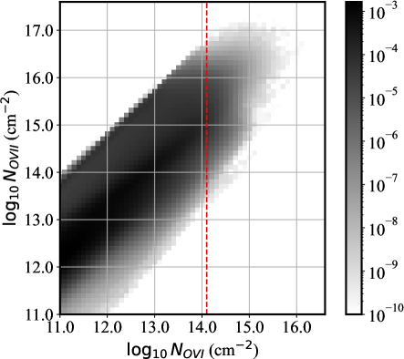
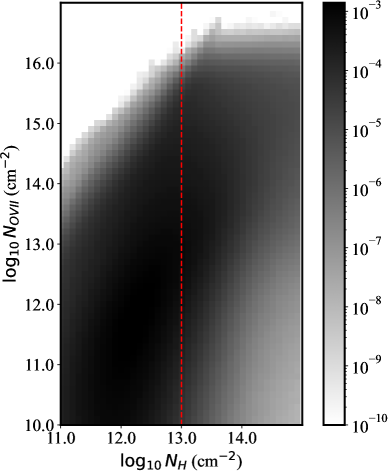
Figure 8: Joint probability distribution of (a) O VII and O VI, and (b) O VII  and H I, from the EAGLE simulations of Wijers et al. (2019). The red lines represent respectively the value of the combined O VI column density detected for absorbers 1 and 2 ($\log N(\mathrm{O~{}VI})=14.1$), which feature a possible XMM-Newton detection of O VII, and the value of a characteristic H I BLA detection for systems 5–8. The distribution represents the number of sightlines in EAGLE with those column density values, and therefore they are not normalized.

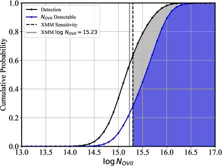
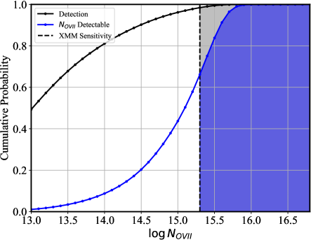
Figure 10: (a) Cumulative distributions for O VII with O VI prior, and (b) for O VII with H I priors. In both panels, black is the cumulative probability distributions for the possible detection of an O VII line, for a fixed value of O VI as in Fig. 9. In blue, for the same distributions, is the cumulative fraction $P_{j}$ of the column density of O VII above a given threshold, according to (7). On the left panel, for a sensitivity of approximately $\log N=15.3$ (15.1) for O VII, EAGLE predicts that a sightline with $\log N_{\text{OVI}}=14.1$ is expected to have a probability $p=0.36$ (0.56) to intercept a sightline with $\log N_{\text{OVII}}\geq 15.3$ (15.1), and it is is sensitive to a fraction $P_{j}\simeq 0.72$ (0.86) of O VII.

6 Discussion and Conclusions

This paper has presented a comprehensive statistical framework for the analysis of X–ray absorption lines from the WHIM, with the goal of drawing inferences on the associated cosmological density of the WHIM, $\Omega_{\text{WHIM,X}}$. The method is based on the search of X–ray absorption lines at fixed redshift where prior FUV observations have identified possible absorption from the lower–temperature WHIM, and the use of joint distribution functions of FUV and X–ray ions based on cosmological simulations.

Within this framework, we have searched the 1ES 1553+113 XMM-Newton spectra for prominent resonant absorption lines from the intervening WHIM. The method we have used is based on the search near 8 fixed redshifts where FUV lines, namely O VI and H I BLAs, had been previously detected by Danforth et al. (2016). The only FUV redshift system with evidence for a WHIM resonant absorption line is $z=0.1876$, where a possible O VII absorption line model is preferred by the data with a 99% level of confidence, approximately corresponding to a 2.6–$\sigma$ significance. Give the limited statistical significance, this detection should be regarded as tentative. Accordingly, we did not attempt any modelling of the physical characteristics of the potential FUV/X–ray absorber, but instead parameterized the associated cosmological inferences as a function of temperature and abundance. If this signal is interpreted as a detection of O VII from the WHIM, such a detection would correspond to a significant fraction ($\Omega_{\mathrm{WHIM,X}}/\Omega_{b}=0.44\pm 0.22$) of the cosmological density of the present–day baryons.

There is no statistically significant evidence of any other X–ray ions along the sightline. To further examine the possibility of WHIM absorption, we performed a stacking of the data for the two O VII and O VIII absorption lines following the methods of Sect. 4.3.5. The results of this analysis are reported in Table 8 and in Figure 4. For O VII from the entire sample of seven independent systems, the significance of detection is at a similar confidence level as redshift system 1 O VII alone. We therefore conclude that there is only marginal evidence for O VII absorption along the sightline to 1ES 1553+113. For O VIII, there is no overall evidence for absorption lines from the stacking of the spectra.

Given the limited statistical significance in the detection of just one O VII system, we also provided an overall upper limit to $\Omega_{\mathrm{WHIM,X}}$ based on the systematic non–detection of WHIM along the sightline to 1ES 1553+113. This upper limit is based on a statistical study of the distribution of X–ray and FUV ions in EAGLE Wijers et al. (2019), and yields a value of $\Omega_{\mathrm{WHIM,X}}/\Omega_{b}\leq 0.90$, assuming 100% O VII fraction, and a chemical abundance of 10% Solar for oxygen. The limit becomes less stringent if the WHIM systems are at a significantly lower temperature, where the ionization fraction of O VII is significantly smaller.

Both the present analysis, and that of Kovács et al. (2019), highlight the importance and the potential of using FUV priors to identify faint X–ray absorption lines, despite the overall difficulty of this task with the current generation of X–ray grating spectrometers. In fact, the use of FUV priors enables the stacking of data at predetermined redshifts with the ensuing increase in sensitivity to absorbing columns, and improves the identification of faint absorption features such as the possible O VII absorption line at $z=0.1876$ identified in this paper.

It is useful to address the question of whether the X–ray absorbing WHIM along the sightline towards 1ES 1553+113 is consistent with the expectation from the EAGLE simulations. Our analysis, largely based on an earlier study by Wijers et al. (2019), uses the joint distribution of O VI and O VII column densities, and that of H I and O VII (see Fig. 8). Given the priors provided by the FUV detections, the probability of an O VII detection at one of the three independent redshifts examined was estimated as $p\simeq 0.3$, depending on the exact value of the assumed sensitivity of the data (see Fig. 10). Since we have at most just one possible detection, and with limited statistical significance, our XMM-Newton data are clearly consistent with the expectation. Specifically, the probability of no detections based on a binomial distribution with $p=0.3$ and $N=3$ tries is 34%, and the probability of one detection is 19%. For the four redshift systems with H I BLA priors, the probability of an O VII line above the sensitivity is smaller, typically of order only a few percent. The systematic non–detection of O VII at these redshifts is again consistent with the EAGLE predictions. The main reasons for the low probability of detection of X–ray absorption are 1) the relatively low quality of the X–ray data limiting the detectable column density level and 2) the relatively short redshift path length probed rendering the number of absorbers low. The currently best X-ray data are only sensitive to O VII column density well in excess of $10^{15}$ cm^-2, while the FUV data are able to detect column densities of order $10^{13}$ cm^-2. In fact, according to Wijers et al. (2019) (see discussion in their Sect. 4.1), EAGLE predicts less than one O VII system for the present 1ES 1553+113 data. This in turn indicates that future searches for the X–ray absorbing WHIM require substantially 1) more sensitive instruments, such as the ones being developed for the future missions Athena (e.g. Barret et al., 2020), Arcus (Smith et al., 2019), Lynx (Gaskin et al., 2019) or HUBS (Cui et al., 2020), and 2) larger path lengths so that the number of intervening absorbers is feasible.

In addition to the search at the FUV redshifts, we also performed a dedicated analysis near two wavelengths where Nicastro et al. (2018) tentatively identified O VII absorption from a blind search of the entire 1ES 1553+113 RGS spectra. For the first wavelength of $\lambda=30.98$Å, the spectra (see bottom panel of Fig. 5) do confirm the presence of an absorption line feature with high statistical significance, even after accounting for the redshift trials in the blind search. For the other feature near the wavelength $\lambda=29.28$Å, we find no statistically significant evidence of absorption (see upper panel of Fig. 5), consistent with the re–analysis done by the same group (Nicastro, 2018), where the initial report of a detection at that redshift was reanalyzed and its significance reduced. The confirmed Nicastro et al. (2018) absorption line, if identified as O VII He–$\alpha$ at $z=0.4339$, would imply a cosmological density of baryons that is indeed consistent with the hypothesis that the missing baryons are in the hot phase of the intergalactic WHIM, for an estimated $\Omega_{\mathrm{WHIM,X}}/\Omega_{b}=0.65\pm 0.11$, assuming typical physical conditions for the absorber. However, Johnson et al. (2019) showed that 1ES 1553+113 is likely a member of a galaxy group at $z=0.433$, and Dorigo Jones et al. (2022) argues that the most likely redshift for 1ES 1553+113 corresponds with that of the X–ray absorber. It is therefore likely that the serendipitous Nicastro et al. (2018) absorption line is intrinsic to the source or associated with the group environment, rather than the WHIM.

Data Availability

The XMM-Newton and Chandra data analyzed in this paper are available from the public NASA W3Browse archive (https://heasarc.gsfc.nasa.gov/cgi-bin/W3Browse/w3browse.pl). Processed data such as spectra and response functions can be obtained by the authors upon request.

References

- Abramowski et al. (2015) Abramowski A., et al., 2015, ApJ, 802, 65
- Ahoranta et al. (2020) Ahoranta J., et al., 2020, A&A, 634, A106
- Ahoranta et al. (2021) Ahoranta J., Finoguenov A., Bonamente M., Tilton E., Wijers N., Muzahid S., Schaye J., 2021, arXiv e-prints, p. arXiv:2109.12146
- Anders & Grevesse (1989) Anders E., Grevesse N., 1989, Geochimica Cosmochimica Acta, 53, 197
- Bahcall & Peebles (1969) Bahcall J. N., Peebles P. J. E., 1969, ApJ, 156, L7
- Barret et al. (2020) Barret D., Decourchelle A., Fabian A., Guainazzi M., Nandra K., Smith R., den Herder J.-W., 2020, Astronomische Nachrichten, 341, 224
- Bertone et al. (2008) Bertone S., Schaye J., Dolag K., 2008, Space Sci. Rev., 134, 295
- Bonamente (2019) Bonamente M., 2019, Journal of Applied Statistics, 46, 1129
- Bonamente (2020) Bonamente M., 2020, Journal of Applied Statistics, 47, 2044
- Bonamente (2022) Bonamente M., 2022, Statistics and Analysis of Scientific Data. Springer, Graduate Texts in Physics, Third Edition
- Bonamente (2023) Bonamente M., 2023, arXiv e-prints, p. arXiv:2302.04011
- Bonamente et al. (2016) Bonamente M., Nevalainen J., Tilton E., Liivamägi J., Tempel E., Heinämäki P., Fang T., 2016, MNRAS, 457, 4236
- Bonamente et al. (2019) Bonamente M., Ahoranta J., Nevalainen J., Holt P., 2019, Research Notes of the AAS, 3, 75
- Buote et al. (2009) Buote D. A., Zappacosta L., Fang T., Humphrey P. J., Gastaldello F., Tagliaferri G., 2009, ApJ, 695, 1351
- Butler Contreras et al. (2023) Butler Contreras A., Lau E. T., Oppenheimer B. D., Bogdán Á., Tillman M., Nagai D., Kovács O. E., Burkhart B., 2023, MNRAS, 519, 2251
- Cagnoni et al. (2004) Cagnoni I., Nicastro F., Maraschi L., Treves A., Tavecchio F., 2004, ApJ, 603, 449
- Cash (1979) Cash W., 1979, ApJ, 228, 939
- Cautun et al. (2014) Cautun M., van de Weygaert R., Jones B. J. T., Frenk C. S., 2014, MNRAS, 441, 2923
- Cen & Ostriker (1999) Cen R., Ostriker J. P., 1999, ApJ, 514, 1
- Cen & Ostriker (2006) Cen R., Ostriker J. P., 2006, ApJ, 650, 560
- Cramer (1946) Cramer H., 1946, Mathematical Methods of Statistics. Princeton University Press, Princeton
- Cui et al. (2020) Cui W., Chen L., Gao B., et al. 2020, J. Low Temp Phys., p. 502–509
- Danforth et al. (2010) Danforth C. W., Keeney B. A., Stocke J. T., Shull J. M., Yao Y., 2010, ApJ, 720, 976
- Danforth et al. (2016) Danforth C. W., et al., 2016, ApJ, 817, 111
- Davé et al. (2001) Davé R., et al., 2001, ApJ, 552, 473
- Dorigo Jones et al. (2022) Dorigo Jones J., et al., 2022, MNRAS, 509, 4330
- Fang et al. (2002) Fang T., Marshall H. L., Lee J. C., Davis D. S., Canizares C. R., 2002, ApJ, 572, L127
- Fang et al. (2007) Fang T., Canizares C. R., Yao Y., 2007, ApJ, 670, 992
- Fang et al. (2010) Fang T., Buote D. A., Humphrey P. J., Canizares C. R., Zappacosta L., Maiolino R., Tagliaferri G., Gastaldello F., 2010, ApJ, 714, 1715
- García et al. (2005) García J., Mendoza C., Bautista M. A., Gorczyca T. W., Kallman T. R., Palmeri P., 2005, ApJS, 158, 68
- Gaskin et al. (2019) Gaskin J. A., et al., 2019, Journal of Astronomical Telescopes, Instruments, and Systems, 5, 021001
- Gatuzz et al. (2015) Gatuzz E., García J., Kallman T. R., Mendoza C., Gorczyca T. W., 2015, ApJ, 800, 29
- Gharaibeh et al. (2011) Gharaibeh M. F., et al., 2011, Journal of Physics B: Atomic, Molecular and Optical Physics, 44, 175208
- Gu et al. (2005) Gu M. F., Schmidt M., Beiersdorfer P., Chen H., Thorn D. B., Träbert E., Behar E., Kahn S. M., 2005, ApJ, 627, 1066
- Hinshaw et al. (2013) Hinshaw G., et al., 2013, ApJS, 208, 19
- Johnson et al. (2019) Johnson S. D., et al., 2019, ApJ, 884, L31
- Kaastra (2017) Kaastra J. S., 2017, Astronomy and Astrophysics, 605, A51
- Kaastra et al. (2006) Kaastra J. S., Werner N., Herder J. W. A. d., Paerels F. B. S., de Plaa J., Rasmussen A. P., de Vries C. P., 2006, ApJ, 652, 189
- Kaastra et al. (2018) Kaastra J. S., de Vries C., den Herder J., 2018
- Kovács et al. (2019) Kovács O. E., Bogdán Á., Smith R. K., Kraft R. P., Forman W. R., 2019, ApJ, 872, 83
- Kraft et al. (2022) Kraft R., et al., 2022, Line Emission Mapper (LEM): Probing the physics of cosmic ecosystems, doi:10.48550/ARXIV.2211.09827, https://arxiv.org/abs/2211.09827
- Martizzi et al. (2018) Martizzi D., et al., 2018, arXiv e-prints,
- Mazzotta et al. (1998) Mazzotta P., Mazzitelli G., Colafrancesco S., Vittorio N., 1998, A&AS, 133, 403
- Mernier et al. (2017) Mernier F., et al., 2017, A&A, 603, A80
- Nevalainen et al. (2017) Nevalainen J., Wakker B., Kaastra J., Bonamente M., Snowden S., Paerels F., de Vries C., 2017, A&A, 605, A47
- Nevalainen et al. (2019) Nevalainen J., et al., 2019, A&A, 621, A88
- Nicastro (2018) Nicastro F., 2018, arXiv e-prints,
- Nicastro et al. (2005) Nicastro F., et al., 2005, ApJ, 629, 700
- Nicastro et al. (2013) Nicastro F., et al., 2013, ApJ, 769, 90
- Nicastro et al. (2018) Nicastro F., et al., 2018, Nature, 558, 406
- Pearce et al. (2021) Pearce F. A., Kay S. T., Barnes D. J., Bahé Y. M., Bower R. G., 2021, MNRAS, 507, 1606
- Protassov et al. (2002) Protassov R., van Dyk D. A., Connors A., Kashyap V. L., Siemiginowska A., 2002, ApJ, 571, 545
- Rasmussen et al. (2007) Rasmussen A. P., Kahn S. M., Paerels F., Herder J. W. d., Kaastra J., de Vries C., 2007, ApJ, 656, 129
- Ren et al. (2014) Ren B., Fang T., Buote D. A., 2014, ApJ, 782, L6
- Ryan-Weber et al. (2009) Ryan-Weber E. V., Pettini M., Madau P., Zych B. J., 2009, MNRAS, 395, 1476
- Schaye (2001) Schaye J., 2001, ApJ, 559, 507
- Schaye et al. (2015) Schaye J., et al., 2015, MNRAS, 446, 521
- Shull et al. (2012) Shull J. M., Smith B. D., Danforth C. W., 2012, ApJ, 759, 23
- Smith et al. (2019) Smith R. K., et al., 2019, in UV, X-Ray, and Gamma-Ray Space Instrumentation for Astronomy XXI. p. 111180W, doi:10.1117/12.2529499
- Stocke et al. (2014) Stocke J. T., et al., 2014, ApJ, 791, 128
- The EAGLE team (2017) The EAGLE team 2017, arXiv e-prints, p. arXiv:1706.09899
- Tilton et al. (2012) Tilton E. M., Danforth C. W., Shull J. M., Ross T. L., 2012, ApJ, 759, 112
- Tuominen et al. (2021) Tuominen T., et al., 2021, A&A, 646, A156
- Verner et al. (1996) Verner D. A., Verner E. M., Ferland G. J., 1996, Atomic Data and Nuclear Data Tables, 64, 1
- Wijers et al. (2019) Wijers N. A., Schaye J., Oppenheimer B. D., Crain R. A., Nicastro F., 2019, arXiv e-prints, p. arXiv:1904.01057
- Wijers et al. (2020) Wijers N. A., Schaye J., Oppenheimer B. D., 2020, MNRAS, 498, 574
- Wilks (1938) Wilks S. S., 1938, Ann. Math. Statist., 9, 60
- Wilks (1943) Wilks S., 1943, Mathematical Statistics. Princeton University Press, Princeton
- Wright (2006) Wright E. L., 2006, PASP, 118, 1711
- Yao et al. (2009) Yao Y., Tripp T. M., Wang Q. D., Danforth C. W., Canizares C. R., Shull J. M., Marshall H. L., Song L., 2009, ApJ, 697, 1784
- Yao et al. (2012) Yao Y., Shull J. M., Wang Q. D., Cash W., 2012, ApJ, 746, 166
- de Vries et al. (2014) de Vries C. P., et al., 2014, in Takahashi T., den Herder J.-W. A., Bautz M., eds, Society of Photo-Optical Instrumentation Engineers (SPIE) Conference Series Vol. 9144, Space Telescopes and Instrumentation 2014: Ultraviolet to Gamma Ray. p. 91440R, doi:10.1117/12.2055712