Perturbation theory challenge for cosmological parameters estimation II.: Matter power spectrum in redshift space

Abstract

Constraining cosmological parameters from large-scale structure observations requires precise and accurate tools to compute its properties. While perturbation theory (PT) approaches can serve this purpose, exploration of large parameter space is challenging due to the potentially large computational cost of such calculations. In this study, we show that a response function approach applied to the regularized PT (RegPT) model at the 2-loop order, plus correction terms induced by redshift space distortion effects, can reduce the runtime by a factor of 50 compared to direct integration. We illustrate the performance of this approach by performing the parameter inference of five fundamental cosmological parameters from the redshift space power spectrum measured from $N$-body simulations as mock measurements, and inferred cosmological parameters are directly compared with parameters used to generate initial conditions of the simulations. From this PT challenge analysis, the constraining power of cosmological parameters and parameter biases are quantified with the survey volume and galaxy number density expected for the Euclid mission at the redshift $z=1$ as a function of the maximum wave-number of data points $k_{\mathrm{max}}$. We find that RegPT with correction terms reproduces the input cosmological parameters without bias up to maximum wave-number $k_{\mathrm{max}}=0.18\,h\,\mathrm{Mpc}^{-1}$. Moreover, RegPT+, which introduces one free parameter to RegPT to handle the damping feature on small scales, delivers the best performance among the examined models and achieves tighter constraints without significant parameter bias for higher maximum wave-number $k_{\mathrm{max}}=0.21\,h\,\mathrm{Mpc}^{-1}$.

I Introduction

The widely accepted scenario in modern cosmology is that quantum fluctuations generated by inflation in the earliest stage of the Universe results in primordial density perturbation and the fluctuations lead to the formation of self-gravitating bound objects called dark halos by gravitational instability. As the Universe evolves, dark halos successively undergo mergers and form structures with a wide range of spatial scales [1]. In the hierarchy of structures, the largest structures are referred to as the large-scale structures (LSS) of the Universe. The spatial clustering of LSS, in particular baryon acoustic oscillation (BAO) [2], is driven by dark matter and is sensitive to the accelerated expansion induced by dark energy. Thus, observations of LSS are the key to understanding the nature of the dark sector [for a review, see 3].

One widely employed probe to map the LSS is the use of the galaxies as tracers of the matter distribution at large cosmological scales. Over the last decade, many such surveys have been built, 6dF Galaxy Survey [4], WiggleZ [5], VIPERS [6], and extended Baryon Acoustic Oscillation Survey [eBOSS; 7]. In the coming era, a new generation of spectroscopic surveys is under preparation, the Subaru Prime Focus Spectrograph [PFS; 8], Dark Energy Spectrograph Instrument [DESI; 9, 10], Euclid [11, 12], and Nancy Grace Roman Space Telescope , which will probe the universe with wider and deeper coverage. These next-generation surveys are promised to advance our understanding of the Universe through precise and accurate measurements of galaxy clustering.

In the practical analysis of galaxy clustering, we rely on statistics to summarize the information of observed galaxy distribution. The most fundamental and widely used statistics is the two-point correlation function or its Fourier space counterpart, the power spectrum. The accurate and precise theoretical model to predict these statistics given a cosmological model is an essential component in the statistical analysis to constrain cosmological models. For this purpose, various approaches have been developed so far. Among such methods, the perturbation theory (PT) of LSS [for a review, see 14] has been commonly employed in practical analysis. In the PT framework, the cosmic matter is approximated as single-stream fluid and the evolution is governed by continuity equation, Euler equation, and Poisson equation. These equations can be expanded with respect to the linear density contrast and this naive approach is called as standard perturbation theory (SPT). SPT is fast enough to apply for statistical inference and the sub-percent level accuracy is achieved up to the mildly non-linear regime. However, SPT is known to exhibit poor convergence of PT expansion and the UV-sensitive behaviors [15, 16]. In order to circumvent this problem and realize better convergence and accuracy, approaches beyond SPT have been developed based on resummation technique in Lagrangian space [17] and in Eulerian space [18, 19, 20].

An alternative to the use of high-order PT calculations to infer the impact of the small scales is to introduce an effective stress tensor in the fluid equations leading to what is referred to as the effective field theory (EFT) of LSS [21, 22, 23]. This approach allows in principle to take into account multi-streaming regime but requires the introduction of free parameters that cannot be computed from first principle.

In all cases, the statistical inference of cosmological parameters from the power spectrum involves theoretical calculations of power spectrum for a large number of sets of cosmological parameters. For example, the standard cosmological model, where the Universe is composed of ordinary matter, cold dark matter (CDM) and the cosmological constant and the geometry is flat, i.e., flat $\Lambda$CDM model, contains at least five cosmological parameters. This number is significantly augmented when one takes into account nuisance parameters for observational systematics, such as the galaxy bias, and the impact of redshift space distortion (RSD) effect[24, 25]. For instance, for a parameter space of three cosmological parameters [26], $\mathcal{O}(10^{5})$ evaluations of statistics were required to perform the parameter inference. A full exploration of the parameter space will be obviously more demanding.

So far, a variety of approaches to predict the power spectrum have been used to explore such large parameter space. Previous works [27, 28, 29, 30] showed that the computational cost of loop correction terms in the SPT expansion could be reduced with the FFTLog algorithm [31]. These methods are formulated up to next-to-leading order (NLO) but have not been implemented at next-to-next-leading order (NNLO). NNLO direct computations have so far been hampered by their computational cost. In order to gain accuracy, EFT approaches have been widely advocated as an alternative to NNLO computations, and applied to full-shape analysis of galaxy power spectrum [32, 33, 34]. The advantage is that their computational cost is indeed comparable to that of NLO computations. The price to pay is the introduction of many extra nuisance parameters to control the impact of the small-scale fluctuations that potentially degrade their constraining power [26]. Finally, it should be noted that simulation-based approaches, e.g., emulator approach [35, 36, 37, 38], are successful in predicting power spectrum down to small scales in a fast manner [39] and have been successfully employed to constrain cosmological parameters from galaxy power spectrum [40]. This is not however the path we choose to follow here.

In general, analytical PT treatments mentioned above have their own limitation, and the robustness of these approaches has to be tested against numerical simulations, in which several non-linear systematics, including gravitational clustering, RSD and galaxy bias, are properly accounted for. However, most of the previous studies have restricted their analysis to the case where cosmological parameters are fixed. For a more practical setup, one would be interested in deriving cosmological constraints, allowing all the parameters in the theoretical models to be free. Nevertheless, in the presence of parameter degeneracies, even if analytical method succeeds in reproducing the observed power spectra, an unbiased parameter estimation is not always guaranteed.

The main goal of this paper is to conduct a cosmology challenge analysis of the perturbation theory, a PT Challenge, extending to redshift space the studies done previously in real space, [26, 41, 42, 43, 44], Since cosmological parameters used to generate the initial conditions of the simulation are known, we can directly compare between the inferred and true values. In this analysis, we mainly focus on the regularized PT approach RegPT [45] with acceleration by the response function expansion fast-RegPT [46]. With the help of the response function, we can significantly reduce the computational cost of the calculation of power spectrum and bispectrum. Through this analysis, we can discuss which model serves the best to give precise and accurate estimates. Further, we determine the extent to which each of PT models/methods can be used as a reliable theoretical template to reproduce safely the cosmological parameters without any systematic bias.

In Section II, we briefly overview the basics of analytical treatments on redshift space power spectrum: SPT, RegPT, IR-resummed EFT. In Section III, we present the fast scheme of RegPT calculation which realizes full fundamental cosmological parameter inference. In Section IV, we present details of PT challenge: statistical analysis and $N$-body simulations, and in Section V, the results of PT challenge are presented. We make concluding remarks in Section VI.

Throughout this paper, we assume flat $\Lambda$CDM Universe. Though we will perform the statistical inference of cosmological parameters, the fiducial cosmological parameters to generate the initial conditions of $N$-body simulations for mock measurements are based on the results of temperature and polarization anisotropies (TT,TE,EE+lowP dataset) measured in Planck 2015 results [47]. The CDM density parameter is $\omega_{\mathrm{cdm}}=0.1198$, the baryon density parameter is $\omega_{\mathrm{b}}=0.02225$, and the massive neutrino density parameter is $\omega_{\nu}=0.00064$. For neutrino, we assume that one of three generations is massive with mass $m_{\nu}=0.06\,\mathrm{eV}$ and the other two are massless. The dark energy density parameter $\Omega_{\mathrm{de}}=0.6844$ and the dark energy is the cosmological constant with the equation of state parameter $w_{\mathrm{de}}=-1$. The Hubble parameter at the present Universe is $H_{0}/(\mathrm{km}\,\mathrm{s}^{-1}\,\mathrm{Mpc}^{-1})=100h=67.27$, which is determined through the flatness $(\omega_{\mathrm{cdm}}+\omega_{\mathrm{b}}+\omega_{\nu})/h^{2}+\Omega_{\mathrm{de}}=1$. The amplitude and tilt of the primordial scalar perturbation is $\log_{10}(10^{10}A_{\mathrm{s}})=3.094$ and $n_{\mathrm{s}}=0.9645$, respectively, with the pivot scale $k_{\mathrm{piv}}=0.05\,\mathrm{Mpc}^{-1}$.

II Theory

In this section, we briefly review the basics of SPT and RegPT and the calculations of power spectrum. In addition to these PT schemes, we present one of EFT treatments: IR-resummed EFT. In the redshift space, non-linear coupling with density and velocity fields has appreciable contributions to the power spectrum. We overview how we can incorporate the effect specific to the redshift space based on the PT framework.

II.1 Standard perturbation theory

Since the density fluctuation is small on large scales and/or at early times, the cosmic matter field can be approximated as a single-stream fluid. Then, the evolution of the cosmic fluid is described by continuity, Euler, and Poisson equations, and the density and velocity divergence field can be expanded in a perturbative manner with respect to the linear density field at the present Universe:

$$\bm{\Psi}(\bm{k};\eta)=\sum_{n=1}^{\infty}e^{n\eta}\bm{\Psi}^{(n)}(\bm{k}),$$ (1)

where $\bm{\Psi}(\bm{k};\eta)=(\delta(\bm{k};\eta),\theta(\bm{k};\eta))$ is the density-velocity doublet, $\delta(\bm{k};\eta)$ and $\theta(\bm{k};\eta)$ are the Fourier transform of the density and velocity divergence field, respectively. The velocity divergence field is normalized as $\theta=-\nabla\cdot\bm{v}/(aHf)$, where $\bm{v}$ is the velocity field, $a$ is the scale factor, $H$ is the Hubble parameter, $f=\differential\ln D_{+}/\differential\ln a$ is the linear growth rate, and $D_{+}(a)$ is the linear growth factor normalized as $D_{+}(a=1)=1$. We have considered the fastest growing mode and adopted Einstein–de Sitter Universe in the expansion, and thus, the time-dependence of the kernel functions is factorizable as $e^{n\eta}$, where $\eta\equiv\ln D_{+}$. The doublet at the linear order ($n=1$) is $\bm{\Psi}^{(1)}(\bm{k})=(\delta_{0}(\bm{k}),\delta_{0}(\bm{k}))$, where $\delta_{0}(\bm{k})$ is the Fourier transform of the linear density field at the present Universe. The $n$-th order term of the doublet $\bm{\Psi}^{(n)}$ is expressed as mode coupling of the Fourier transform of the linear density field due to non-linear gravitational evolution:

$$\Psi_{a}^{(n)}(\bm{k})= \int\frac{\differential[3]{q_{1}}}{(2\pi)^{3}}\cdots\int\frac{\differential[3]{q_{n}}}{(2\pi)^{3}}(2\pi)^{3}\delta_{\mathrm{D}}(\bm{k}-\bm{q}_{1\cdots n})$$

$$\times\ F_{a}^{(n)}(\bm{q}_{1},\ldots,\bm{q}_{n})\delta_{0}(\bm{q}_{1})\cdots\delta_{0}(\bm{q}_{n}),$$ (2)

where $\delta_{\mathrm{D}}$ is the Dirac delta function, $\bm{q}_{1\cdots n}\equiv\bm{q}_{1}+\cdots+\bm{q}_{n}$, and $F_{a}^{(n)}$ are symmetrized kernel functions and the explicit expression is derived via the recursion relation [see, e.g., 18].

Based on the PT framework, one can also compute the statistics of the density and velocity divergence field in a perturbative manner. As a working example, let us consider the most fundamental statistics to characterize the cosmic field: power spectrum $P_{ab}$ and bispectrum $B_{abc}$, which is the Fourier space version of 2-point and 3-point correlation functions, respectively. The definitions are given as

$$\langle\Psi_{a}(\bm{k};\eta)\Psi_{b}(\bm{k}^{\prime};\eta)\rangle\equiv(2\pi)^{3}\delta_{\mathrm{D}}(\bm{k}+\bm{k}^{\prime})P_{ab}(k;\eta),$$ (3)

$$\langle\Psi_{a}(\bm{k}_{1};\eta)\Psi_{b}(\bm{k}_{2};\eta)\Psi_{c}(\bm{k}_{3};\eta)\rangle\\ \equiv(2\pi)^{3}\delta_{\mathrm{D}}(\bm{k}_{123})B_{abc}(\bm{k}_{1},\bm{k}_{2},\bm{k}_{3};\eta),$$ (4)

where the subscript ($a,b,c$) denotes the density $\delta$ or the velocity divergence $\theta$. Based on the perturbative expressions (Eq. 1), the power spectrum and the bispectrum can be calculated as the loop expansion:

$$P_{ab}(k;\eta)=P_{ab,\text{tree}}(k,\eta)+P_{ab,\text{1-loop}}(k,\eta)+\cdots,$$ (5)

$$B_{abc}(\bm{k}_{1},\bm{k}_{2},\bm{k}_{3};\eta)=B_{abc,\text{tree}}(\bm{k}_{1},\bm{k}_{2},\bm{k}_{3};\eta)\\ +B_{abc,\text{1-loop}}(\bm{k}_{1},\bm{k}_{2},\bm{k}_{3};\eta)+\cdots.$$ (6)

These expansions are ordered with respect to the linear power spectrum at the present Universe $P_{0}(k)$, which is defined as

$$\langle\delta_{0}(\bm{k})\delta_{0}(\bm{k}^{\prime})\rangle\equiv(2\pi)^{3}\delta_{\mathrm{D}}(\bm{k}+\bm{k}^{\prime})P_{0}(k).$$ (7)

The tree level (LO) terms of power spectrum and bispectrum ($P_{ab,\text{tree}}$ and $B_{abc,\text{tree}}$) are proportional to the linear power spectrum and the square of the linear power spectrum, respectively. Next, the 1-loop level (NLO) terms ($P_{ab,\text{1-loop}}$ and $B_{abc,\text{1-loop}}$) require the loop integral with the external wave-vector and the integrand for power spectrum (bispectrum) contains the square (cubic) power of the linear power spectrum. In general, $n$-loop terms involve $3n-1$ dimensional integrals and the power of the linear power spectrum in the integrands is $n+1$ for power spectrum and $n+2$ for bispectrum. In practice, one needs to truncate the infinite series of the expansion to compute the power spectrum and the bispectrum, and in this paper, terms up to 2-loop orders are considered for the power spectrum calculations.

II.2 Regularized perturbation theory

In order to improve the convergence of the SPT expansion, the resummation technique, which reorganizes the terms of the SPT expansion, has been developed. Among the resummed PT frameworks, we consider the regularized perturbation theory (RegPT) [45], which utilizes the multi-point propagators to reorganize the SPT expansion, i.e., $\Gamma$-expansion [19].

First, we introduce the expressions of multi-point propagators, which are defined as the response of the density and velocity divergence fields with respect to the linear density field. The $(n+1)$-point propagator $\Gamma_{a}^{(n)}$ is defined as

$$\frac{1}{n!}\left\langle\frac{\delta^{n}\Psi_{a}(\bm{k};\eta)}{\delta\delta_{0}(\bm{k}_{1})\cdots\delta\delta_{0}(\bm{k}_{n})}\right\rangle\\ \equiv\delta_{\mathrm{D}}(\bm{k}-\bm{k}_{1\cdots n})(2\pi)^{-3(n-1)}\Gamma_{a}^{(n)}(\bm{k}_{1},\ldots\bm{k}_{n};\eta).$$ (8)

The expression of the propagator is given as

$$\Gamma_{a}^{(n)}(\bm{k}_{1},\ldots,\bm{k}_{n};\eta)$$

$$=\Gamma_{a,\text{tree}}^{(n)}(\bm{k}_{1},\ldots,\bm{k}_{n};\eta)+\sum_{p=1}^{\infty}\Gamma_{a,p\text{-loop}}^{(n)}(\bm{k}_{1},\ldots,\bm{k}_{n};\eta),$$ (9)

$$\Gamma_{a,\text{tree}}^{(n)}(\bm{k}_{1},\ldots,\bm{k}_{n};\eta)\equiv e^{n\eta}F_{a}^{(n)}(\bm{k}_{1},\ldots,\bm{k}_{n})$$ (10)

$$\Gamma_{a,p\text{-loop}}^{(n)}(\bm{k}_{1},\ldots,\bm{k}_{n};\eta)\equiv$$

$$e^{(n+2p)\eta}c_{p}^{(n)}\int\frac{\differential[3]{q_{1}}}{(2\pi)^{3}}\cdots\int\frac{\differential[3]{q_{p}}}{(2\pi)^{3}}$$

$$\times F_{a}^{(n)}(\bm{q}_{1},-\bm{q}_{1},\ldots,\bm{q}_{p},-\bm{q}_{p},\bm{k}_{1},\ldots,\bm{k}_{n})P_{0}(q_{1})\cdots P_{0}(q_{p})$$ (11)

$$\equiv e^{(n+2p)\eta}\bar{\Gamma}^{(n)}_{a,p\text{-loop}}(\bm{k}_{1},\ldots,\bm{k}_{n}),$$ (12)

where $c_{p}^{(n)}\equiv\binom{n+2p}{n}(2n-1)!!$. There is a notable feature that the propagator has an asymptotic form at high-$k$ limit [19]:

$$\lim_{k\to\infty}\Gamma_{a}^{(n)}(\bm{k}_{1},\ldots,\bm{k}_{n};\eta)=\\ \exp\left[-\frac{k^{2}e^{2\eta}\sigma_{\mathrm{d}}^{2}}{2}\right]\Gamma_{a,\text{tree}}^{(n)}(\bm{k}_{1},\ldots,\bm{k}_{n};\eta),$$ (13)

where $k\equiv|\bm{k}_{1}+\cdots+\bm{k}_{n}|$, $\sigma_{\mathrm{d}}^{2}$ is the dispersion of the displacement field:

$$\sigma_{\mathrm{d}}^{2}(k)\equiv\int_{0}^{k_{\Lambda}(k)}\frac{\differential q}{6\pi^{2}}P_{0}(q),$$ (14)

and we have introduced the UV cutoff scale $k_{\Lambda}(k)$ and adopted $k_{\Lambda}(k)=k/2$ to match the result of $N$-body simulations [45]. This displacement dispersion controls the damping feature on small scales and it is known that making $\sigma_{\mathrm{d}}$ a free parameter improves the fit to the $N$-body simulation results [26]. We refer to this one-parameter extended RegPT model as RegPT+.

It is possible to express the statistics of density and velocity fields with the propagator expansion. The power spectrum and the bispectrum based on RegPT are formally expressed as the infinite series [19]:

$$\langle\Psi_{a}(\bm{k};\eta)\Psi_{b}(\bm{k}^{\prime};\eta)\rangle= \delta_{\mathrm{D}}(\bm{k}+\bm{k}^{\prime})\sum_{p=1}^{\infty}p!\int\frac{\differential[3]{q_{1}}\cdots\differential[3]{q_{p}}}{(2\pi)^{3p}}\delta_{\mathrm{D}}(\bm{k}-\bm{q}_{1\ldots p})$$

$$\times\Gamma_{a}^{(p)}(\bm{q}_{1},\ldots\bm{q}_{p};\eta)\Gamma_{b}^{(p)}(\bm{q}_{1},\ldots\bm{q}_{p};\eta)P_{0}(q_{1})\cdots P_{0}(q_{p}),$$ (15)

$$\langle\Psi_{a}(\bm{k}_{1};\eta)\Psi_{b}(\bm{k}_{2};\eta)\Psi_{c}(\bm{k}_{3};\eta)\rangle= \sum_{\alpha,\beta,\gamma}\binom{\alpha+\beta}{\alpha}\binom{\beta+\gamma}{\beta}\binom{\gamma+\alpha}{\gamma}\alpha!\beta!\gamma!\int\frac{\differential[3]{p_{1}}\cdots\differential[3]{p_{\alpha}}}{(2\pi)^{3(\alpha-1)}}\frac{\differential[3]{q_{1}}\cdots\differential[3]{q_{\beta}}}{(2\pi)^{3(\beta-1)}}\frac{\differential[3]{r_{1}}\cdots\differential[3]{r_{\gamma}}}{(2\pi)^{3(\gamma-1)}}$$

$$\times\delta_{\mathrm{D}}(\bm{k}_{1}-\bm{p}_{1\ldots\alpha}-\bm{q}_{1\ldots\beta})\delta_{\mathrm{D}}(\bm{k}_{2}+\bm{q}_{1\ldots\beta}-\bm{r}_{1\ldots\gamma})\delta_{\mathrm{D}}(\bm{k}_{3}+\bm{r}_{1\ldots\gamma}+\bm{p}_{1\ldots\alpha})$$

$$\times\Gamma_{a}^{(\alpha+\beta)}(\bm{p}_{1},\ldots,\bm{p}_{\alpha},\bm{q}_{1},\ldots,\bm{q}_{\beta};\eta)\Gamma_{b}^{(\beta+\gamma)}(-\bm{q}_{1},\ldots,-\bm{q}_{\beta},\bm{r}_{1},\ldots,\bm{r}_{\gamma};\eta)$$

$$\times\Gamma_{c}^{(\gamma+\alpha)}(-\bm{r}_{1},\ldots,-\bm{r}_{\gamma},-\bm{p}_{1},\ldots,-\bm{p}_{\alpha};\eta)$$

$$\times P_{0}(p_{1})\cdots P_{0}(p_{\alpha})P_{0}(q_{1})\cdots P_{0}(q_{\beta})P_{0}(r_{1})\cdots P_{0}(r_{\gamma}),$$ (16)

where the summation in Eq. (16) runs over non-negative integers with the constraint that at most one of the indices ($\alpha,\beta,\gamma$) is zero. Similarly to the SPT expansion, one needs to truncate the expansion. Hereafter, we suppress the time variable $\eta$ for simplicity. For more explicit construction of the power spectrum and bispectrum calculations respectively at the 2- and 1-loop orders, refer to Refs. [45, 48].

II.3 Redshift space power spectrum

The peculiar motion of galaxies along the line-of-sight direction is known to induce the anisotropy onto the power spectrum observed via spectroscopic surveys, referred to as the RSD effect, and this effect must be taken into account for the analysis of the power spectrum measurements. The redshift space power spectrum is enhanced on large scales due to a coherent infall toward gravitational potential well, which is referred to as the Kaiser effect [25]. The non-linear version of the Kaiser formula is given as

$$P_{\mathrm{Kaiser}}^{(\mathrm{S})}(k,\mu)=P_{\delta\delta}(k)+2f\mu^{2}P_{\delta\theta}(k)+f^{2}\mu^{4}P_{\theta\theta}(k),$$ (17)

where $P_{\delta\delta}$, $P_{\delta\theta}$, and $P_{\theta\theta}$ is the density auto-, the density-velocity cross-, and the velocity auto-spectra in the real space, respectively, and $\mu$ is the directional cosine with respect to the line-of-sight direction. Hereafter, we take the $z$-axis as the line-of-sight direction. Furthermore, the non-linear coupling of density and velocity fields give rise to additional contributions at small scales [49]. This effect can be modeled as a perturbative manner using the cumulant expansion and the formalism is presented in Ref. [50], which is referred to as the Taruya–Nishimichi–Saito (TNS) correction, and further extended with RegPT [48]. The resultant power spectrum in the redshift space based on RegPT is given as

$$P^{(\mathrm{S})}_{\text{RegPT}}(k,\mu)= D_{\mathrm{FoG}}(k\mu f\sigma_{\mathrm{v}})$$

$$\times\left[P_{\delta\delta}(k)+2f\mu^{2}P_{\delta\theta}(k)+f^{2}\mu^{4}P_{\theta\theta}(k)\right.$$

$$\left.+A(k,\mu)+B(k,\mu)\right],$$ (18)

where $D_{\mathrm{FoG}}$ is the damping function due to the Finger-of-God (FoG) effect and will be discussed later, and two correction terms denoted as $A(k,\mu)$ and $B(k,\mu)$ are introduced. These correction terms are referred to as TNS terms. The explicit expressions of $A$- and $B$-terms are given as

$$A(k,\mu)= (k\mu f)\int\frac{\differential[3]p}{(2\pi)^{3}}\frac{\mu_{p}}{p}$$

$$\times\left[B_{\sigma}(\bm{p},\bm{k}-\bm{p},-\bm{k})-B_{\sigma}(\bm{p},\bm{k},-\bm{k}-\bm{p})\right],$$ (19)

$$B(k,\mu)= (k\mu f)^{2}\int\frac{\differential[3]p}{(2\pi)^{3}}F(\bm{p})F(\bm{k}-\bm{p}),$$ (20)

$$F(\bm{p})\equiv \frac{\mu_{p}}{p}\left[P_{\delta\theta}(p)+f\frac{\mu_{p}}{p}P_{\theta\theta}(p)\right],$$ (21)

where the cross-bispectrum $B_{\sigma}$ is defined as

$$\left\langle\theta(\bm{k}_{1})\left\{\delta(\bm{k}_{2})+f\frac{\mu_{2}}{k_{2}}\theta(\bm{k}_{2})\right\}\left\{\delta(\bm{k}_{3})+f\frac{\mu_{3}}{k_{3}}\theta(\bm{k}_{3})\right\}\right\rangle$$

$$\equiv(2\pi)^{3}\delta_{\mathrm{D}}(\bm{k}_{1}+\bm{k}_{2}+\bm{k}_{3})B_{\sigma}(\bm{k}_{1},\bm{k}_{2},\bm{k}_{3}).$$ (22)

These expressions do not depend on the direction of the wave-vector $\bm{k}$, and thus, we take $\bm{k}=(0,0,k)$ and the directional cosine as $\mu_{p}=(\bm{k}\cdot\bm{p})/(kp)=p_{z}/p$. The expression of the $A$-term is written as the integrals of density and velocity bispectra:

$$A(k,\mu)= \sum_{n=1}^{3}\sum_{a,b=1}^{2}\mu^{2n}f^{a+b-1}\frac{k^{3}}{(2\pi)^{2}}\int_{0}^{\infty}\!\!\differential r\int_{-1}^{+1}\!\!\differential x$$

$$\times\left[A^{n}_{ab}(r,x)B_{2ab}(\bm{p},\bm{k}-\bm{p},-\bm{k})\right.$$

$$\left.+\tilde{A}^{n}_{ab}(r,x)B_{2ab}(\bm{k}-\bm{p},\bm{p},-\bm{k})\right]$$

$$\equiv \sum_{n=1}^{3}\mu^{2n}A_{2n}(k),$$ (23)

where $r$ and $x$ are the dimensionless variables defined as $r=p/k$ and $x=(\bm{p}\cdot\bm{k})/(pk)$. As a notation, we also assign an integer to the subscript: $a=1$ denotes the density field $\delta$ and $a=2$ denotes the velocity divergence field $\theta$. Next, the $B$-term is expressed as the integrals of the power spectra:

$$B(k,\mu)= \sum_{n=1}^{4}\sum_{a,b=1}^{2}\mu^{2n}(-f)^{a+b}\frac{k^{3}}{(2\pi)^{2}}\int_{0}^{\infty}\!\!\differential r\int_{-1}^{+1}\!\!\differential x$$

$$\times B^{n}_{ab}(r,x)\frac{P_{a2}(k\sqrt{1+r^{2}-2rx})P_{b2}(kr)}{(1+r^{2}-2rx)^{a}}$$

$$\equiv \sum_{n=1}^{4}\mu^{2n}B_{2n}(k).$$ (24)

The explicit expressions of auxiliary functions ($A_{ab}^{n},\tilde{A}_{ab}^{n},B_{ab}^{n}$) are found in Ref. [50]. Hereafter, we consider the power spectrum in the redshift space at the 2-loop order, and thus, density auto-, velocity auto-, and density-velocity cross-spectra in Eq. (18) are computed at the 2-loop order. For TNS terms, the bispectra in the $A$-term and the power spectra in the $B$-term should be computed at the 1-loop order to be consistent. It is possible to derive the expression of the redshift space power spectrum based on SPT at the 1-loop order in the same manner and the derivation is described in Appendix A.

At small scales, the random motion of galaxies suppresses the structures, which is referred to as the FoG effect [24]. The damping effect is well explained by the phenomenological model, which introduces the damping function $D_{\mathrm{FoG}}(k\mu f\sigma_{\mathrm{v}})$ to control the overall amplitude of the power spectrum and the functional form is taken as Gaussian or Lorentzian form:

$$D_{\mathrm{FoG}}(x)=\begin{cases}\exp(-x^{2})&(\text{Gaussian}),\\ (1+x^{2}/2)^{-2}&(\text{Lorentzian}).\end{cases}$$ (25)

In most of the models, the velocity dispersion $\sigma_{\mathrm{v}}$ is treated as a free parameter and can be calculated at the linear order as

$$\sigma^{2}_{\mathrm{v,L}}=\int_{0}^{\infty}\frac{\differential q}{6\pi^{2}}P_{\mathrm{L}}(q;z),$$ (26)

where $P_{\mathrm{L}}(k;z)=e^{2\eta(z)}P_{0}(k)$ is the linear power spectrum at the redshift $z$. We also consider another functional form with one free parameter $\gamma$ [51]:

$$D_{\mathrm{FoG}}(x)=\left(1+\frac{x^{2}}{\gamma}\right)^{-\gamma}.$$ (27)

This FoG model becomes Lorentzian FoG for $\gamma=2$ and asymptotes to Gaussian FoG with $\gamma\to\infty$. Thus, this model contains the Gaussian and Lorentzian FoGs and has more flexibility. Hereafter, we refer to this FoG model as “$\gamma$ FoG”.

II.4 IR-resummed effective field theory

The EFT provides a practical way to compute the power spectrum down to small scales ($\gtrsim 0.3\,h\,\mathrm{Mpc}^{-1}$) once free parameters are calibrated with $N$-body simulations or marginalized over as nuisance parameters in comparing its predictions with simulations/observations. In order to examine the performance of the EFT against PT models, we adopt the latter approach and consider specifically the IR-resummed EFT model, where the damping of BAO feature due to the large-scale bulk motion is corrected in the perturbative approach [52, 53, 54]. Here, we describe the power spectrum based on IR-resummed EFT at the 1-loop order. Although our primary focus is to test the 2-loop PT predictions, the 1-loop EFT is now being used for parameter inference on observational data. Thus, comparing its performance with those of the 2-loop PT would provide a useful guideline for future applications to observations.

First, we divide the linear power spectrum $P_{\mathrm{L}}(k)$ into the wiggle and smooth parts. The smooth part $P_{\mathrm{L}}^{\mathrm{nw}}(k)$ is obtained by smoothing the linear power spectrum with no-wiggle power spectrum:

$$P_{\mathrm{L}}^{\mathrm{nw}}(k)= P_{\mathrm{EH}}(k)\frac{1}{\sqrt{2\pi}\log_{10}\lambda}\int\differential(\log_{10}q)\frac{P_{\mathrm{L}}(q)}{P_{\mathrm{EH}}(q)}$$

$$\times\exp\left[-\frac{(\log_{10}k-\log_{10}q)^{2}}{2(\log_{10}\lambda)^{2}}\right],$$ (28)

where we adopt the smoothing scale $\lambda=10^{0.25}\,h\,\mathrm{Mpc}^{-1}$ [53] and $P_{\mathrm{EH}}$ is no-wiggle power spectrum from the fitting formula in Ref. [55]. The wiggle part $P_{\mathrm{L}}^{\mathrm{w}}(k)$ is obtained by taking the residual:

$$P_{\mathrm{L}}^{\mathrm{w}}(k)=P_{\mathrm{L}}(k)-P_{\mathrm{L}}^{\mathrm{nw}}(k).$$ (29)

The expression for IR-resummed EFT power spectrum [56] is given as

$$P^{(\mathrm{S})}_{\text{EFT}}(k,\mu)= P^{\mathrm{nw}}_{\mathrm{L}}(k,\mu)+P^{\mathrm{nw}}_{\text{1-loop}}(k,\mu)$$

$$+P^{\mathrm{nw}}_{\mathrm{ctr}}(k,\mu)+P_{\mathrm{shot}}$$

$$+e^{-k^{2}\Sigma^{2}_{\mathrm{tot}}(\mu)}\left[(1+k^{2}\Sigma^{2}_{\mathrm{tot}}(\mu))P^{\mathrm{w}}_{\mathrm{L}}(k,\mu)\right.$$

$$\left.+P^{\mathrm{w}}_{\text{1-loop}}(k,\mu)+P^{\mathrm{w}}_{\mathrm{ctr}}(k,\mu)\right],$$ (30)

where $P_{\mathrm{shot}}$ is the constant shot noise term. The total damping function $\Sigma^{2}_{\mathrm{tot}}(\mu)$ is defined as

$$\Sigma^{2}_{\mathrm{tot}}(\mu) =[1+f\mu^{2}(2+f)]\Sigma^{2}+f^{2}\mu^{2}(\mu^{2}-1)\delta\Sigma^{2},$$ (31)

$$\Sigma^{2} =\frac{1}{6\pi^{2}}\int_{0}^{k_{S}}\!\!\differential q\,P^{\mathrm{nw}}_{\mathrm{L}}(q)\left[1-j_{0}(qr_{s})+2j_{2}(qr_{s})\right],$$ (32)

$$\delta\Sigma^{2} =\frac{1}{2\pi^{2}}\int_{0}^{k_{S}}\!\!\differential q\,P^{\mathrm{nw}}_{\mathrm{L}}(q)j_{2}(qr_{s}),$$ (33)

where $r_{s}$ is the sound horizon scale, and $j_{0}$ and $j_{2}$ are 0th and 2nd order spherical Bessel functions. We adopt $k_{S}=0.2\,h^{-1}\,\mathrm{Mpc}$ [56]. For the counter term $P_{\mathrm{ctr}}(k,\mu)$, we adopt the following form:

$$P_{\mathrm{ctr}}(k,\mu)= -2\tilde{c}_{0}k^{2}P_{\mathrm{L}}(k)-2\tilde{c}_{2}f\mu^{2}k^{2}P_{\mathrm{L}}(k)$$

$$-2\tilde{c}_{4}f^{2}\mu^{4}k^{2}P_{\mathrm{L}}(k)$$

$$+\tilde{c}_{\nabla^{4}\delta}f^{4}\mu^{4}k^{4}(1+f\mu^{2})^{2}P_{\mathrm{L}}(k),$$ (34)

where four parameters ($\tilde{c}_{0}$, $\tilde{c}_{2}$, $\tilde{c}_{4}$, $\tilde{c}_{\nabla^{4}\delta}$) are introduced. For 1-loop correction and counter terms, smooth and wiggle parts are obtained by regarding the expressions as the functional of the linear power spectrum and plugging the smoothed and wiggly linear power spectra into SPT expressions:

$$P^{\mathrm{nw}}_{\text{1-loop}} \equiv P_{\text{1-loop}}[P^{\mathrm{nw}}_{\mathrm{L}}],$$ (35)

$$P^{\mathrm{w}}_{\text{1-loop}} \equiv P_{\text{1-loop}}[P_{\mathrm{L}}]-P_{\text{1-loop}}[P^{\mathrm{nw}}_{\mathrm{L}}],$$ (36)

$$P^{\mathrm{nw}}_{\mathrm{ctr}} \equiv P_{\mathrm{ctr}}[P^{\mathrm{nw}}_{\mathrm{L}}],$$ (37)

$$P^{\mathrm{w}}_{\mathrm{ctr}} \equiv P_{\mathrm{ctr}}[P_{\mathrm{L}}]-P_{\mathrm{ctr}}[P^{\mathrm{nw}}_{\mathrm{L}}].$$ (38)

II.5 Alcock–Paczyński effect

When converting the galaxy position and redshift into the comoving coordinate, one needs to assume cosmological parameters relevant to the geometry of the Universe. The cosmological parameters are varied for inference but due to the high computational cost, the redshift-distance conversion is performed only once with fiducial cosmological parameter set. The wrong fiducial cosmological parameters induce spurious anisotropy to the power spectrum. This effect is called as Alcock–Paczyński (AP) effect [57]. The distortion is proportional to the Hubble distance for the line-of-sight direction and the angular diameter distance for the direction perpendicular to the line-of-sight direction. Then, we define AP parameters:

$$\alpha_{\parallel}=\frac{D_{H}}{D_{H}^{\mathrm{fid}}}\frac{r_{d}^{\mathrm{fid}}}{r_{d}},\ \alpha_{\perp}=\frac{D_{M}}{D_{M}^{\mathrm{fid}}}\frac{r_{d}^{\mathrm{fid}}}{r_{d}},$$ (39)

where $r_{d}$ is the sound horizon at the drag epoch, $D_{M}(z)=(1+z)D_{A}(z)$ is the proper motion distance, $D_{H}(z)=c/H(z)$ is the Hubble distance, $D_{A}(z)$ is the angular diameter distance, $c$ is the speed of light, $H(z)$ is the Hubble parameter, and the superscript “fid” represents the value computed with the fiducial cosmology. Accordingly, the distorted power spectrum is given as

$$P^{(\mathrm{S})}_{\mathrm{AP}}(k,\mu) =\left(\frac{r_{d}^{\mathrm{fid}}}{r_{d}}\right)^{3}\frac{1}{\alpha_{\parallel}\alpha_{\perp}^{2}}P^{(\mathrm{S})}(q,\nu),$$ (40)

$$q =\frac{k}{\alpha_{\perp}}\left[1+\mu^{2}\left(\frac{\alpha_{\perp}^{2}}{\alpha_{\parallel}^{2}}-1\right)\right]^{\frac{1}{2}},$$ (41)

$$\nu =\frac{\mu\alpha_{\perp}}{\alpha_{\parallel}}\left[1+\mu^{2}\left(\frac{\alpha_{\perp}^{2}}{\alpha_{\parallel}^{2}}-1\right)\right]^{\frac{1}{2}}.$$ (42)

This power spectrum is an observable when the fiducial cosmology is fixed to derive the redshift-distance relation.

The information on anisotropic clustering signal is expressed by the pair of $\alpha_{\parallel}$ and $\alpha_{\perp}$. On the other hand, different combinations are introduced in the literature. Among such pairs, we consider the dilation (warping) parameter $\alpha$ ($\epsilon$) [58], the volume-averaged distance $D_{V}(z)$, and the AP parameter $F_{\mathrm{AP}}(z)$:

$$\alpha \equiv\alpha_{\parallel}^{\frac{1}{3}}\alpha_{\perp}^{\frac{2}{3}},$$ (43)

$$\epsilon \equiv\left(\frac{\alpha_{\parallel}}{\alpha_{\perp}}\right)^{\frac{1}{3}}-1,$$ (44)

$$D_{V}(z) \equiv(zD_{M}^{2}(z)D_{H}(z))^{\frac{1}{3}},$$ (45)

$$F_{\mathrm{AP}}(z) \equiv D_{M}(z)/D_{H}(z).$$ (46)

The dilation parameter $\alpha$ corresponds to the isotropic deformation and thus can be constrained from the BAO scale. On the other hand, the warping parameter $\epsilon$ describes the anisotropic deformation and the change of this parameter has more impact on the anisotropic moments. Another pair is the volume-averaged distance $D_{V}(z)$ and the AP parameter $F_{\mathrm{AP}}(z)$, which are widely employed in previous galaxy clustering analyses.

III Fast schemes for the redshift space power spectrum

In the practical parameter inference from the power spectrum measurements, a fast methodology is critical to explore the large parameter space. Typically, a runtime of less than a few minutes for each cosmological model is required. In order to realize fast calculations of the redshift space power spectrum at the 2-loop order, we employ the response function approach to speed up the computations of the density and velocity power spectra at the 2-loop order and the TNS correction terms.

The codes to compute the power spectrum with TNS correction terms are implemented in the framework of Eclairs [59] and will be publicly available at the github repositry .

III.1 Response function approach

In this section, we describe the response function approach to speed up the calculations of the power spectrum and the bispectrum [for details, see Ref. 46] and implement this approach for calculations of the TNS correction terms. In general, the expressions of the power spectrum based on PT approaches can be regarded as the functionals with respect to the linear power spectrum. In the response function approach, the PT expressions are expanded with functional derivatives and if the fiducial cosmology is close to the target cosmology, the power spectrum for the target cosmology is well approximated with the expansion up to the leading order:

$$P_{ab}(k;\bm{\theta}^{\mathrm{tar}},\sigma_{\mathrm{d}}^{\mathrm{tar}})\simeq P_{ab}(k;\bm{\theta}^{\mathrm{fid}},\sigma_{\mathrm{d}}^{\mathrm{tar}})\\ +\int\differential q\frac{\delta P_{ab}[P_{0};\bm{\theta}^{\mathrm{fid}},\sigma_{\mathrm{d}}^{\mathrm{tar}}]}{\delta P_{0}(q)}\delta P_{0}(q),$$ (47)

$$B_{abc}(\bm{k}_{1},\bm{k}_{2},\bm{k}_{3};\bm{\theta}^{\mathrm{tar}},\sigma_{\mathrm{d}}^{\mathrm{tar}})\simeq B_{abc}(\bm{k}_{1},\bm{k}_{2},\bm{k}_{3};\bm{\theta}^{\mathrm{fid}},\sigma_{\mathrm{d}}^{\mathrm{tar}})\\ +\int\differential q\frac{\delta B_{abc}[P_{0};\bm{\theta}^{\mathrm{fid}},\sigma_{\mathrm{d}}^{\mathrm{tar}}]}{\delta P_{0}(q)}\delta P_{0}(q),$$ (48)

where $\delta P_{ab}/\delta P_{0}$ and $\delta B_{abc}/\delta P_{0}$ are the response functions of the power spectrum and the bispectrum, respectively, $\bm{\theta}^{\mathrm{tar}}$ and $\bm{\theta}^{\mathrm{fid}}$ are sets of cosmological parameters for target and fiducial cosmologies, respectively, and $\delta P_{0}(q)=P_{0}^{\mathrm{tar}}(q)-P_{0}^{\mathrm{fid}}(q)$ is the difference of linear power spectra between the fiducial and target cosmologies. Once the fiducial spectra and response functions are precomputed, the computational cost to evaluate spectra at target cosmologies is just to perform the one-dimensional integrations (second terms of the right hand sides in Eqs. 47 and 48). Since the original expressions at the 2-loop order involve five-dimensional integrations, this response function approach considerably reduces the computational costs. Note that the displacement dispersion $\sigma_{\mathrm{d}}$ is always evaluated at the target cosmology because the cosmology dependence of the displacement dispersion is incorporated without cost after the precomputations.

The redshift space power spectrum (Eq. 18) has contributions from three 2-loop spectra ($P_{\delta\delta}$, $P_{\delta\theta}$, $P_{\theta\theta}$) and TNS corrections, and all of them involve five-dimensional integrations, which hamper fast predictions essential to the statistical inference. For 2-loop spectra, we can make use of the response function approach and the computations require only one-dimensional integrations, which can be computed within a few seconds in general. The most time-consuming part is five-dimensional integrations in the $A$-terms: the 1-loop bispectrum contains three-dimensional integrations and for the $A$-term, the bispectra are further integrated twice. The response function approach is also applicable to TNS correction terms. With the response function expansion, the bispectra in the $A$-terms and the power spectra in the $B$-terms can be calculated in a fast manner, and both of $A$- and $B$-terms become three-dimensional integrations. The response function approach is not applied to the entire $A$- and $B$-terms because the variation of $\sigma_{\mathrm{d}}$ is not easily incorporated. This reduction of computational time makes the analytical PT scheme feasible for cosmological parameter estimation with the redshift space power spectrum.

III.2 Validation

In order to validate our fast scheme, we compare the results with the fast approach and direct integrations. We follow the validation procedure in Ref. [46]. First, we generate $10$ fiducial and $10$ target cosmological parameter sets around Planck 2015 best-fit cosmological parameters, which are homogeneously sampled with the latin hypercube design [61]. The parameter ranges of fiducial and target cosmological parameters are described in Section III.B of Ref. [46]. For fiducial sets, we precompute power spectra, bispectra, and response functions and for each target set, we select the nearest fiducial set according to the distance between fiducial and target linear power spectra, which is denoted as $d$ (see Eq. 22 of Ref. [46] for definition). In Ref. [46], we have found that the response function approach reproduces the results with direct integrations with the accuracy of $0.5\%$ for power spectra and $2\%$ for bispectra up to $0.3\,h\,\mathrm{Mpc}^{-1}$.

Here, we apply the response function technique to the TNS correction terms and investigate the accuracy. For power spectra, the number of sampling for wave-numbers should be small but sufficient to reconstruct the full shape of spectra. We employ the following adaptive sampling scheme:

$$\begin{cases}[10^{-3},10^{-2}]\,h\,\mathrm{Mpc}^{-1}&(\Delta\log k=\mathrm{const.},n_{k}=10),\\ [10^{-2},0.3]\,h\,\mathrm{Mpc}^{-1}&(\Delta k=\mathrm{const.},n_{k}=80),\\ [0.3,1]\,h\,\mathrm{Mpc}^{-1}&(\Delta\log k=\mathrm{const.},n_{k}=30),\\ \end{cases}$$ (49)

where $n_{k}$ is the number of sampling. For the intermediate range, we use linear spacing to capture the BAO feature, otherwise the log-equally spaced sampling is employed. If the spectra with arbitrary wave-numbers are necessary, we employ cubic spline. In $A$-term calculations, bispectra with specific configurations $(\bm{k}_{1},\bm{k}_{2},\bm{k}_{3})=(\bm{p},\bm{k}-\bm{p},-\bm{k})$ are required. The range of the wave-number $k$ is $(10^{-3},1)\,h\,\mathrm{Mpc}^{-1}$ with log-equally spaced $300$ wave-numbers. For integration with respect to the wave-vector $\bm{p}$, numerical integrations are performed with Gaussian quadrature for $r=p/k$ and $x=(\bm{p}\cdot\bm{k})/(pk)$ and the number of sampling is $n_{r}=600$ and $n_{x}=10$, respectively.

Figure 1 shows the results with the response function approach for $10$ target models and the ratios with respect to the direct integration results. The accuracy of $A$-term calculations is about $1\%$ at all scales. There is a noisy feature around $k=0.07\,h\,\mathrm{Mpc}^{-1}$ but this originates from zero-crossing of direct integration results. Similarly, Figure 2 shows the results for $B$-terms. The accuracy for the $B$-terms is more stable and well within $1\%$ for all scales.

In the practical analysis, instead of two-dimensional power spectrum $P^{\mathrm{(S)}}(k,\mu)$, the multipole expansion is widely used to characterize the anisotropy. The $\ell$-th order multipole moment is defined as

$$P_{\ell}(k)\equiv\frac{2\ell+1}{2}\int_{-1}^{+1}\!\!\differential\mu\,\mathcal{P}_{\ell}(\mu)P^{\mathrm{(S)}}(k,\mu),$$ (50)

where $\mathcal{P}_{\ell}$ is the Lengendre polynomial of order $\ell$. Another representation of anisotropic power spectrum is wedges [62] which are mean power spectrum with a given range of the directional cosine:

$$P_{w}(k)\equiv\frac{1}{\mu_{\mathrm{max}}^{w}-\mu_{\mathrm{min}}^{w}}\int_{\mu_{\mathrm{min}}^{w}}^{\mu_{\mathrm{max}}^{w}}\!\!\differential\mu\,P^{\mathrm{(S)}}(k,\mu),$$ (51)

where $[\mu_{\mathrm{min}}^{w},\mu_{\mathrm{max}}^{w}]$ is the range of the bin. Figures 3 and 4 demonstrate the performance of the response function approach for multipoles and wedges, respectively. For multipoles, monopole ($\ell=0$), quadrupole ($\ell=2$), and hexadecapole ($\ell=4$) moments are considered. For wedges, we consider two sets of wedge bins:

$$[\mu_{\mathrm{min}}^{w},\mu_{\mathrm{max}}^{w}]=\begin{cases}\left[0,\frac{1}{3}\right],\left[\frac{1}{3},\frac{2}{3}\right],\left[\frac{2}{3},1\right]&(\text{3 wedges}),\\ \left[0,\frac{1}{2}\right],\left[\frac{1}{2},1\right]&(\text{2 wedges}).\end{cases}$$ (52)

The response function approach has been employed to compute all 2-loop spectra and TNS correction terms. The accuracy of multipoles and wedges is well within $0.5\%$ up to $k=0.3\,h\,\mathrm{Mpc}^{-1}$. Therefore, the fast scheme can be applied to practical analysis.

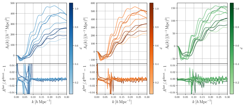
Figure 1: The $A$-terms at the redshift $z=0.9$ computed with the response function approach. The upper panels show $A$-terms for the 10 target models and the color corresponds to the distance from the nearest fiducial model, which is defined in Eq. (22) of Ref. [46]. The lower panels show the fractional difference with respect to the results with direct integration.

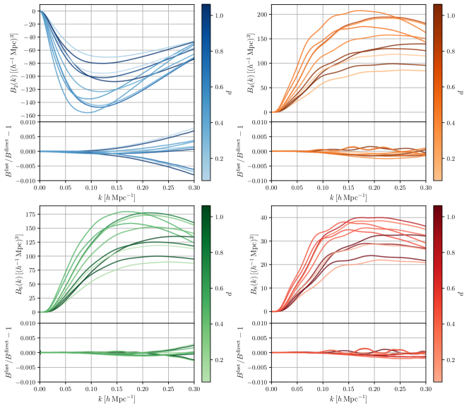
Figure 2: The $B$-terms at the redshift $z=0.9$ computed with the response function approach. The configuration of the lower panels and the color is the same as Figure 1.

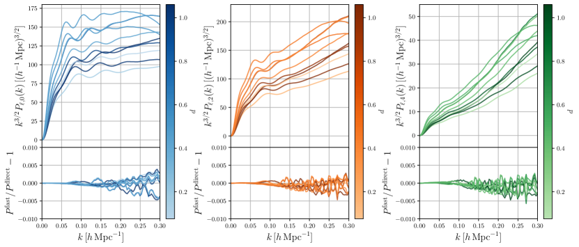
Figure 3: The monopole, quadrupole, and hexadecapole moments at the redshift $z=0.9$ computed with the response function approach. The configuration of the lower panels and the color is the same as Figure 1.

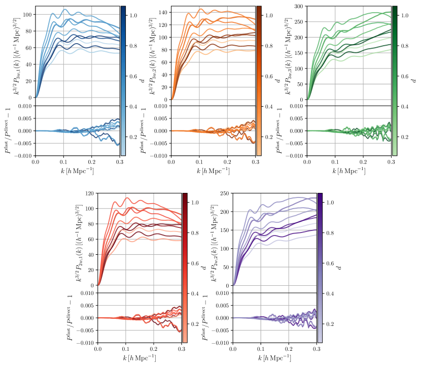
Figure 4: The wedge power spectra at the redshift $z=0.9$ computed with the response function approach. The upper three figures show the results with 3 wedges $[0,1/3],[1/3,2/3],[2/3,1]$ and the lower two figures show the results with 2 wedges $[0,1/2],[1/2,1]$. The configuration of the lower panels and the color is the same as Figure 1.

IV Perturbation theory challenge in redshift space

Here, we describe the PT challenge analysis and present details of $N$-body simulations for mock measurements of the redshift space power spectrum and theoretical templates used in the analysis.

IV.1 Mock measurement of the power spectrum

First, we prepare the realistic mock measurements of the power spectrum in the cosmological parameter inference. The baseline $N$-body simulation is presented in Ref. [63] and here we briefly summarize specifications of the simulation. The gravitational evolution of the matter density field is solved by the Tree-PM code L-Gadget-2 [64]. The initial condition is generated at the redshift $z_{\mathrm{ini}}=15$ based on the second-order Lagrangian PT [65, 66, 67, 68] with the transfer function calculated with the Boltzmann solver CAMB [69]. Furthermore, the Fourier amplitude and phase of initial conditions are determined based on the “paired and fixed” approach [70] to suppress the cosmic variance. The employed cosmological parameters are the best-fit values of Planck 2015 results [47], which are listed in Section I. The volume of the simulation box is $V_{s}=2048^{3}\,(h^{-1}\,\mathrm{Mpc})^{3}$ with periodic boundary condition and the number of particle is $N=2048^{3}$.

Hereafter, we employ the particle snapshot at the redshift $z=0.900902$. We construct the density field with regular grids, where the number of grid is $1024$ on a side, with cloud-in-cell mass assignment and then apply fast Fourier transform to obtain the Fourier space density field. For power spectrum measurements, Fourier amplitude for each mode is summed up for the given range of bins: for multipoles,

$$\hat{P}_{\ell}(k_{i})=\frac{2\ell+1}{N_{k_{i}}}\sum_{k\in[k_{i}-\Delta k/2,k_{i}+\Delta k/2]}|\tilde{\delta}(k_{\parallel},\bm{k}_{\perp})|^{2}\mathcal{P}_{\ell}(\mu),$$ (53)

and for wedges,

$$\hat{P}_{w}(k_{i})=\frac{1}{N_{k_{i},w}}\sum_{\begin{subarray}{c}k\in[k_{i}-\Delta k/2,k_{i}+\Delta k/2]\\ |\mu|\in[\mu^{w}_{\mathrm{min}},\mu^{w}_{\mathrm{max}}]\end{subarray}}|\tilde{\delta}(k_{\parallel},\bm{k}_{\perp})|^{2},$$ (54)

where $\tilde{\delta}$ is the Fourier transform of the density field, $\mu=k_{\parallel}/k$, $k=\sqrt{k_{\parallel}^{2}+k_{\perp}^{2}}$ and the number of modes is calculated by counting the modes for the three-dimensional regular grids:

$$N_{k_{i}} =\sum_{k\in[k_{i}-\Delta k/2,k_{i}+\Delta k/2]}1,$$ (55)

$$N_{k_{i},w} =\sum_{\begin{subarray}{c}k\in[k_{i}-\Delta k/2,k_{i}+\Delta k/2]\\ |\mu|\in[\mu^{w}_{\mathrm{min}},\mu^{w}_{\mathrm{max}}]\end{subarray}}1.$$ (56)

Here, we consider the linearly spaced bins with $\Delta k=0.01\,h\,\mathrm{Mpc}^{-1}$. If the width is sufficiently small compared with $k$, the estimator converges. However, on large scales, i.e., small $k$, the number of available modes is limited and the discreteness of modes impacts the estimation of the power spectrum. In order to incorporate the finite grid effect, in the model prediction, we take the sum of modes as performed in the estimators (Eqs. 53 and 54) with replacing $|\tilde{\delta}|^{2}$ with the model template $P^{(\mathrm{S})}$ [48].

We assume that the likelihood follows the multi-variate Gaussian distribution: for multipoles,

$$-2\log\mathcal{L}_{\text{multipoles}}(\bm{\theta};k_{\mathrm{max}})=$$

$$\sum_{\ell,\ell^{\prime}}\sum_{i,j}^{k_{i},k_{j}<k_{\mathrm{max}}}\left[\hat{P}_{\ell}(k_{i})-P_{\ell}(\bm{\theta};k_{i})\right]\mathrm{Cov}_{\ell,\ell^{\prime}}^{-1}(k_{i},k_{j})$$

$$\times\left[\hat{P}_{\ell^{\prime}}(k_{j})-P_{\ell^{\prime}}(\bm{\theta};k_{j})\right]+\text{const.}$$ (57)

$$\equiv\chi^{2}_{\text{multipoles}}+\text{const.}$$ (58)

and for wedges,

$$-2\log\mathcal{L}_{\text{wedges}}(\bm{\theta};k_{\mathrm{max}})=$$

$$\sum_{w,w^{\prime}}\sum_{i,j}^{k_{i},k_{j}<k_{\mathrm{max}}}\left[\hat{P}_{w}(k_{i})-P_{w}(\bm{\theta};k_{i})\right]\mathrm{Cov}_{w,w^{\prime}}^{-1}(k_{i},k_{j})$$

$$\times\left[\hat{P}_{w^{\prime}}(k_{j})-P_{w^{\prime}}(\bm{\theta};k_{j})\right]+\text{const.}$$ (59)

$$\equiv\chi^{2}_{\text{wedges}}+\text{const.},$$ (60)

where $\bm{\theta}$ is the set of cosmological and nuisance parameters, $k_{\mathrm{max}}$ is the maximum wave-number to exclude small-scale data points, $\hat{P}_{\ell}(k_{i})$ and $\hat{P}_{w}(k_{i})$ are binned multipoles and wedges measured from the simulation, and $P_{\ell}(\bm{\theta};k_{i})$ and $P_{w}(\bm{\theta};k_{i})$ are model predictions of multipoles and wedges, and $\chi^{2}_{\text{multipoles}}$ and $\chi^{2}_{\text{wedges}}$ are the chi-squares for multipoles and wedges, respectively.

IV.2 Covariance matrix

In the actual observations, galaxies are used as a tracer of the matter distribution, and thus, the galaxy power spectrum is employed in the analysis. Though we are interested in how our approach performs for the matter power spectrum without uncertainty relevant to the galaxy bias, it is important to take into account the shot noise due to the finite number of observed galaxies. Hence, we include the effective shot noise term with angular dependence:

$$\frac{1}{n_{\mathrm{g}}^{\mathrm{eff}}}(\mu)=\frac{(1+f\mu^{2})^{2}}{(b_{\mathrm{g}}+f\mu^{2})^{2}}\frac{1}{n_{\mathrm{g}}},$$ (61)

where $b_{\mathrm{g}}=1.41$ is the linear galaxy bias and $n_{\mathrm{g}}=8.4\times 10^{-4}\,(h^{-1}\,\mathrm{Mpc})^{-3}$ is the galaxy number density, which are expected values in Euclid survey at redshift $z=1$ [12]. Assuming furthermore that the field is Gaussian distributed, the covariance matrix of multipoles is given by (e.g., [50, 72, 73])

$$\mathrm{Cov}_{\ell,\ell^{\prime}}(k_{i},k_{j})=\delta_{ij}\frac{2}{N_{k_{i}}}\frac{(2\ell+1)(2\ell^{\prime}+1)}{2}\int_{k_{i}-\Delta k/2}^{k_{i}+\Delta k/2}\frac{4\pi k^{2}\differential k}{V_{k_{i}}}\int_{-1}^{+1}\!\!\differential\mu\,\mathcal{P}_{\ell}(\mu)\mathcal{P}_{\ell^{\prime}}(\mu)\left[P^{(\mathrm{S})}_{\mathrm{L,FoG}}(k,\mu)+\frac{1}{n_{\mathrm{g}}^{\mathrm{eff}}}(\mu)\right]^{2},$$ (62)

where $V_{k_{i}}=(4\pi/3)[(k_{i}+\Delta k/2)^{3}-(k_{i}-\Delta k/2)^{3}]$, $N_{k_{i}}=V_{k_{i}}V_{s}/(2\pi)^{3}$ is the number of modes within the bin. The power spectrum $P^{(\mathrm{S})}_{\mathrm{L,FoG}}(k,\mu)$ is at linear order with the Lorentzian FoG damping function:

$$P^{(\mathrm{S})}_{\mathrm{L,FoG}}(k,\mu)=D_{\mathrm{FoG}}^{\text{Lorentzian}}(k\mu f\sigma_{\mathrm{v,L}})(1+f\mu^{2})^{2}P_{\mathrm{L}}(k).$$ (63)

Though the linear model underestimates the power spectrum at small scales where non-linear evolution predominates, the damping due to the FoG effect is strong on small scales and the shot noise is dominant in the covariance matrix. Thus, the linear model yields reasonable estimates of the covariance matrix. Similarly, the covariance matrix for wedges is given by [72, 73]

$$\mathrm{Cov}_{w,w^{\prime}}(k_{i},k_{j})=\delta_{ij}\delta_{w,w^{\prime}}\frac{2}{N_{k_{i}}\Delta\mu^{w}}\int_{k_{i}-\Delta k/2}^{k_{i}+\Delta k/2}\frac{4\pi k^{2}\differential k}{V_{k_{i}}}\int_{\mu^{w}_{\mathrm{min}}}^{\mu^{w}_{\mathrm{max}}}\!\!\frac{\differential\mu}{\Delta\mu^{w}}\left[P^{(\mathrm{S})}_{\mathrm{L,FoG}}(k,\mu)+\frac{1}{n_{\mathrm{g}}^{\mathrm{eff}}}(\mu)\right]^{2},$$ (64)

where $\Delta\mu^{w}\equiv\mu^{w}_{\mathrm{max}}-\mu^{w}_{\mathrm{min}}$ is the wedge bin width. Note that these covariance matrices are calculated once with fiducial cosmological parameters and thus, the cosmological dependence is not considered in the cosmological parameter inference.

IV.3 Markov chain Monte-Carlo analysis

Our PT challenge for cosmological parameter estimation employs Markov chain Monte-Carlo (MCMC) technique to compute the posterior distribution of parameters. To be specific, we use the Affine invariant ensemble sampler emcee [74, 75]. As a baseline model, we adopt RegPT at the 2-loop order with Lorentzian FoG, the data vector consisting of 3 multipoles ($\ell=0,2,4$), and the AP effect incorporated. We also consider the various cases for PT modeling and data vectors in the MCMC analysis;

PT model

RegPT (2-loop), RegPT+ (2-loop), IR-resummed EFT (1-loop)

Data vector

3 multipoles ($\ell=0,2,4$), 2 multipoles ($\ell=0,2$), 3 wedges ($\left[0,1/3\right],\left[1/3,2/3\right],\left[2/3,1\right]$), 2 wedges ($\left[0,1/2\right],\left[1/2,1\right]$)

FoG

Lorentzian, Gaussian, $\gamma$ FoGs

AP effect

Considered or ignored

Table 1 summarizes the cases we examined in the PT challenge analysis, in which the IR-resummed EFT at 1-loop order is included as a reference model to clarify the performance of 2-loop PT models. We vary the maximum wave-number $k_{\mathrm{max}}$, i.e., the smallest scale of the data points used in the analysis, from $0.12\,h\,\mathrm{Mpc}^{-1}$ to $0.30\,h\,\mathrm{Mpc}^{-1}$ by the step of $0.03\,h\,\mathrm{Mpc}^{-1}$. The results based on 1-loop PT models (RegPT, RegPT+, and SPT) are discussed in Appendix B.

In the subsequent MCMC analysis, we consider five cosmological parameters ($\omega_{\mathrm{cdm}},\omega_{\mathrm{b}},h,A_{\mathrm{s}},n_{\mathrm{s}}$) plus nuisance parameters, which are described in Table 1. All the models involve the linear bias parameter $b_{1}$ as a nuisance parameter. Since the measured power spectrum is the matter power spectrum, the true value of the bias parameter in this analysis is unity. On the other hand, we assume that there is no velocity bias. In order to incorporate the linear bias in the models, $f$ and $P_{ab}$ in Eq. (18) are replaced with $\beta\equiv f/b_{1}$ and $b_{1}^{2}P_{ab}$, respectively. The TNS correction terms scale with the linear bias as

$$A(k,\mu;f)\to b_{1}^{3}A(k,\mu;\beta),$$ (65)

$$B(k,\mu;f)\to b_{1}^{4}B(k,\mu;\beta).$$ (66)

The velocity dispersion parameter $\sigma_{\mathrm{v}}$ controls the scale of FoG damping and this parameter is required by all the models with RegPT and RegPT+. RegPT+ introduces the new parameter, the dispersion displacement parameter $\sigma_{\mathrm{d}}$, which improves the modeling of small-scale power spectra. If $\gamma$ FoG is selected, the nuisance parameter $\gamma$ is included and this parameter determines the shape of FoG damping. The IR-resummed EFT models introduce coefficients of counter terms ($\tilde{c}_{0},\tilde{c}_{2},\tilde{c}_{4},\tilde{c}_{\nabla^{4}\delta}$) and the shot noise term $P_{\mathrm{shot}}$ as nuisance parameters. In the cases of 2 multipoles and 2 wedges, we do not include the parameter $\tilde{c}_{4}$, which is the coefficient of the counter term proportional to $\mu^{4}$, because this term is less constrained due to the limited sampling in the $\mu$-direction.

We add prior information for $\omega_{\mathrm{b}}$ and $n_{\mathrm{s}}$, which are only poorly constrained with the redshift space power spectrum. For both parameters, the prior distribution is Gaussian with mean values given by the fiducial ones and standard deviations of $n_{\mathrm{s}}$ and $\omega_{\mathrm{b}}$ inferred respectively by the Planck 2015 result and the constraints brought by big-bang nucleosynthesis and observations of primordial deutrium abundance [76]. Note that for the $\gamma$ FoG, the sampled parameter is $\gamma^{-1}$ instead of $\gamma$ because the $\gamma$ FoG asymptotes to the Gaussian FoG with $\gamma\to\infty$, i.e., $\gamma^{-1}\to 0$, and the correspondence becomes clearer with $\gamma^{-1}$. For other parameters, we assume flat prior distributions and they are summarized in Table 2. All the chains are run with 80 walkers. For convergence of the chains, the sampler is run until the length of chains is 50 times longer than the auto-correlation time for all cosmological parameters .

Table 1: Descriptions of models of RegPT and RegPT+ at 2-loop order and IR-resummed EFT at 1-loop order. The label describes the components of the model: the PT model (RegPT, RegPT+, or IR-resummed EFT), the functional form of FoG damping (Lorentzian, Gaussian, or $\gamma$ FoGs), and the data vector (3/2 multipoles or 3/2 wedges).

Label	Model	Data vector	AP	FoG	Nuisance parameters
RPT-L-3$\ell$	RegPT	3 Multipoles ($\ell=0,2,4$)	✓	Lorentzian	$b_{1},\sigma_{\mathrm{v}}$
RPT-G-3$\ell$	RegPT	3 Multipoles ($\ell=0,2,4$)	✓	Gaussian	$b_{1},\sigma_{\mathrm{v}}$
RPT-$\gamma$-3$\ell$	RegPT	3 Multipoles ($\ell=0,2,4$)	✓	$\gamma$ FoG	$b_{1},\sigma_{\mathrm{v}},\gamma^{-1}$
RPT(no AP)-L-3$\ell$	RegPT	3 Multipoles ($\ell=0,2,4$)	—	Lorentzian	$b_{1},\sigma_{\mathrm{v}}$
RPT-L-2$\ell$	RegPT	2 Multipoles ($\ell=0,2$)	✓	Lorentzian	$b_{1},\sigma_{\mathrm{v}}$
RPT-L-3$w$	RegPT	3 Wedges ($\left[0,1/3\right],\left[1/3,2/3\right],\left[2/3,1\right]$)	✓	Lorentzian	$b_{1},\sigma_{\mathrm{v}}$
RPT-L-2$w$	RegPT	2 Wedges ($\left[0,1/2\right],\left[1/2,1\right]$)	✓	Lorentzian	$b_{1},\sigma_{\mathrm{v}}$
RPT+-L-3$\ell$	RegPT+	3 Multipoles ($\ell=0,2,4$)	✓	Lorentzian	$b_{1},\sigma_{\mathrm{v}},\sigma_{\mathrm{d}}$
RPT+-G-3$\ell$	RegPT+	3 Multipoles ($\ell=0,2,4$)	✓	Gaussian	$b_{1},\sigma_{\mathrm{v}},\sigma_{\mathrm{d}}$
RPT+-$\gamma$-3$\ell$	RegPT+	3 Multipoles ($\ell=0,2,4$)	✓	$\gamma$ FoG	$b_{1},\sigma_{\mathrm{v}},\gamma^{-1},\sigma_{\mathrm{d}}$
RPT+(no AP)-L-3$\ell$	RegPT+	3 Multipoles ($\ell=0,2,4$)	—	Lorentzian	$b_{1},\sigma_{\mathrm{v}},\sigma_{\mathrm{d}}$
RPT+-L-2$\ell$	RegPT+	2 Multipoles ($\ell=0,2$)	✓	Lorentzian	$b_{1},\sigma_{\mathrm{v}},\sigma_{\mathrm{d}}$
RPT+-L-3$w$	RegPT+	3 Wedges ($\left[0,1/3\right],\left[1/3,2/3\right],\left[2/3,1\right]$)	✓	Lorentzian	$b_{1},\sigma_{\mathrm{v}},\sigma_{\mathrm{d}}$
RPT+-L-2$w$	RegPT+	2 Wedges ($\left[0,1/2\right],\left[1/2,1\right]$)	✓	Lorentzian	$b_{1},\sigma_{\mathrm{v}},\sigma_{\mathrm{d}}$
EFT-3$\ell$	IR-resummed EFT	3 Multipoles ($\ell=0,2,4$)	✓	—	$b_{1},\tilde{c}_{0},\tilde{c}_{2},\tilde{c}_{4},\tilde{c}_{\nabla^{4}\delta},P_{\mathrm{shot}}$
EFT-2$\ell$	IR-resummed EFT	2 Multipoles ($\ell=0,2$)	✓	—	$b_{1},\tilde{c}_{0},\tilde{c}_{2},\tilde{c}_{\nabla^{4}\delta},P_{\mathrm{shot}}$
EFT-3$w$	IR-resummed EFT	3 Wedges ($\left[0,1/3\right],\left[1/3,2/3\right],\left[2/3,1\right]$)	✓	—	$b_{1},\tilde{c}_{0},\tilde{c}_{2},\tilde{c}_{4},\tilde{c}_{\nabla^{4}\delta},P_{\mathrm{shot}}$
EFT-2$w$	IR-resummed EFT	2 Wedges ($\left[0,1/2\right],\left[1/2,1\right]$)	✓	—	$b_{1},\tilde{c}_{0},\tilde{c}_{2},\tilde{c}_{\nabla^{4}\delta},P_{\mathrm{shot}}$

Table 2: Priors and fiducial value for cosmological and nuisance parameters. The symbol $\mathcal{N}(\mu,\sigma)$ is the Gaussian distribution with the mean $\mu$ and the standard deviation $\sigma$ and the symbol $\mathcal{U}(a,b)$ is the flat distribution in the range of $(a,b)$.

Parameter	Prior	Fiducial value
$\omega_{\mathrm{cdm}}$	$\mathcal{U}(0,\infty)$	$0.1198$
$\omega_{\mathrm{b}}$	$\mathcal{N}(0.02225,0.0005)$	$0.02225$
$n_{\mathrm{s}}$	$\mathcal{N}(0.9645,0.0049)$	$0.9645$
$h$	$\mathcal{U}(0,\infty)$	$0.6727$
$\ln(10^{10}A_{\mathrm{s}})$	$\mathcal{U}(0,\infty)$	$3.094$
$b_{1}$	$\mathcal{U}(0,\infty)$	$1$
$\sigma_{\mathrm{d}}$, $\sigma_{\mathrm{v}}$, $\gamma^{-1}$, $P_{\mathrm{shot}}$	$\mathcal{U}(0,\infty)$	—
$\tilde{c}_{0}$, $\tilde{c}_{2}$, $\tilde{c}_{4}$, $\tilde{c}_{\nabla^{4}\delta}$	$\mathcal{U}(-\infty,\infty)$	—

V Results

In this Section, we present the results of the PT challenge analysis. First, as a demonstration of the accuracy of PT schemes, we show power spectra with fiducial and best-fit cosmological parameters. Next, in order to quantify the performance of the PT schemes, we introduce three measures: Figure of Bias (FoB), Figure of Merit (FoM), and reduced chi-square. FoB corresponds to the normalized distance between the inferred and fiducial cosmological parameters, and FoM indicates the constraining power of parameters. The reduced chi-square is the goodness of fit, i.e. how close the PT scheme predictions are to the data.

Here, we only show results for primary models with a part of maximum wave-numbers. The complete results including all models are found in Supplemental Material .

V.1 Fiducial and best-fit power spectra

Before the parameter inference, we present predictions with fiducial cosmological parameters, which are used to generate the initial condition of the $N$-body simulations, based on RegPT, RegPT+, and IR-resummed EFT. The bias parameter is fixed as unity ($b_{1}=1$) and other nuisance parameters are fit with the likelihood functions defined in Eqs. (57) and (59). Figures 5, 6, and 7 show the fiducial multipoles, 3 wedges, and 2 wedges, respectively, in comparison with the simulation result. The maximum wave-number is $k_{\mathrm{max}}=0.21\,h\,\mathrm{Mpc}^{-1}$ and the data points with $k<k_{\mathrm{max}}$ are used to fit nuisance parameters. In general, all of the models yield good fits to the simulation spectra. For multipoles, the difference is clear for hexadecapoles; Gaussian FoG significantly underestimates the hexadecapole moment, and the IR-resummed EFT can reproduce the hexadecopole the best among the models examined. For 3 wedges and 2 wedges, there is an overshoot at large scale for IR-resummed EFT because counter terms are adjusted to fit small-scale power, where the covariance is small, and as a result, the accuracy at the large scale is degraded.

Next, the cosmological parameters are varied and the posterior distributions are inferred with the MCMC analysis. We define the best-fit parameters as the ones which yield the maximum of the posterior in the chain . Figures 8, 9, and 10 show the best-fit multipoles, 3 wedges, and 2 wedges, respectively, in comparison with the simulation result. The cosmological and nuisance parameters are determined to maximize the posterior functions . At the cost of the large-scale power, most of models try to fit the small-scale power whose errors are small. As a result, the best-fit power spectra are better matched with simulations at the intermediate scale ($k=0.1\text{--}0.2\,h\,\mathrm{Mpc}^{-1}$) compared with fiducial power spectra.

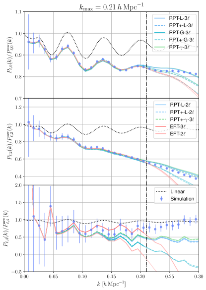
Figure 5: The monopole (upper panel), quadrupole (middle panel), and hexadecapole (lower panel) moments computed with fiducial cosmological parameters. The cyan points and black dotted lines correspond to the simulation result and the linear prediction, respectively. The nuisance parameters are fit to maximize the likelihood and the maximum wave-number of data points in the fitting is $k_{\mathrm{max}}=0.21\,h\,\mathrm{Mpc}^{-1}$, which is indicated as the black dot-dashed vertical line. Note that the hexadecapole moments of the models with 2 multipoles are not shown because they are not used for fitting.

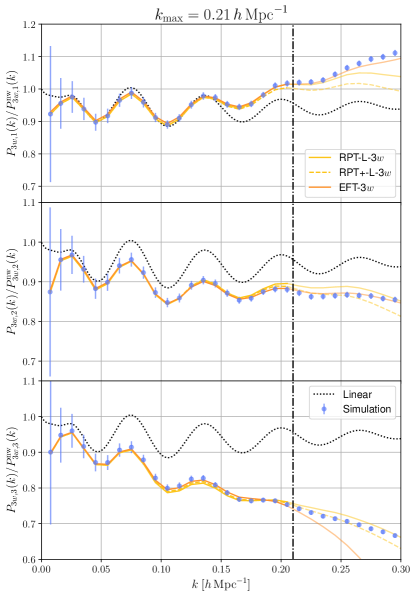
Figure 6: The same as Figure 5 but for 3 wedges.

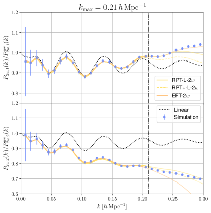
Figure 7: The same as Figure 5 but for 2 wedges.

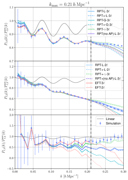
Figure 8: The monopole (upper panel), quadrupole (middle panel), and hexadecapole (lower panel) moments computed with best-fit parameters. The cyan points and black dotted lines correspond to the simulation result and the linear prediction, respectively. The cosmological and nuisance parameters are fit to maximize the posterior and the maximum wave-number of data points in the fitting is $k_{\mathrm{max}}=0.21\,h\,\mathrm{Mpc}^{-1}$, which is indicated as the black dot-dashed vertical line. Note that the hexadecapole moments of the models with 2 multipoles are not shown because they are not used for fitting.

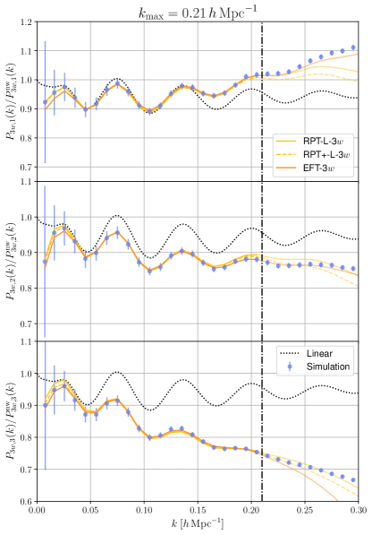
Figure 9: The same as Figure 8 but for 3 wedges.

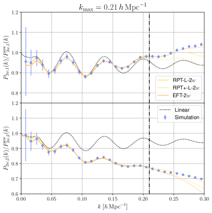
Figure 10: The same as Figure 8 but for 2 wedges.

V.2 Constraints on cosmological and derived parameters

Here, we present examples of parameter inference results. Figures 11, 12, and 13 show constraints of cosmological and nuisance parameters for RegPT, RegPT+ and IR-resummed EFT, respectively. The FoG damping function for RegPT and RegPT+ is Lorentzian and the data vector is 3 multipoles. As the general trend, the parameter constraints become tighter for larger $k_{\mathrm{max}}$ since more small-scale data are incorporated in the parameter inference. On the other hand, when the aggressive $k_{\mathrm{max}}$, e.g., $k_{\mathrm{max}}=0.30\,h\,\mathrm{Mpc}^{-1}$ for RegPT, is chosen, the validity of the PT scheme ceases to be adequate due to a stronger non-linearity in the power spectra, and the predictions are no longer reliable. As a result, the inferred parameters are strongly biased. This feature is common in all the models.

Next, Figures 14, 15, and 16 show constraints on derived parameters. Overall, the similar feature to cosmological parameters appears. At low $k_{\mathrm{max}}$, the parameters are consistent with fiducial values but the constraining power is weak. On the other hand, increasing high $k_{\mathrm{max}}$ leads to tight constraints but biased inference because the PT schemes become less reliable. This trend is clearer for $b_{1}\sigma_{8}$ and $f\sigma_{8}$, which correspond to the amplitudes of density and velocity power spectra. These parameters are sensitive to the small-scale power spectra, and strongly biased with aggressive $k_{\mathrm{max}}$. In contrast, AP parameters $(\alpha_{\perp},\alpha_{\parallel},F_{\mathrm{AP}})$ and the distance scale ($D_{V}/r_{d}$) are more robustly determined even with high $k_{\mathrm{max}}$. These parameters are constrained with the geometry information at large scales, and thus, the parameter bias is less significant even for high $k_{\mathrm{max}}$.

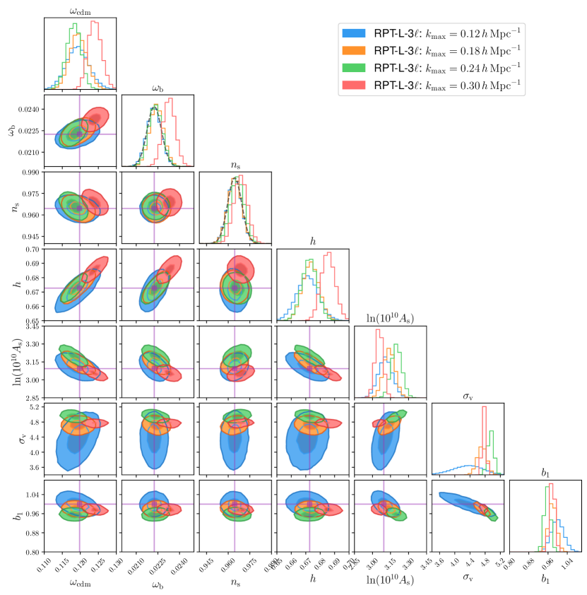
Figure 11: Constraints of cosmological and nuisance parameters inferred with RegPT with Lorentzian FoG and 3 multipoles for $k_{\mathrm{max}}=0.12,0.18,0.24,0.30\,h\,\mathrm{Mpc}^{-1}$. The inner and outer ellipses correspond to the $1\text{-}\sigma$ and $2\text{-}\sigma$ confidence levels, respectively. The purple lines correspond to fiducial values. The prior distributions of $\omega_{\mathrm{b}}$ and $n_{\mathrm{s}}$ are shown as black dashed lines. The unit of $\sigma_{\mathrm{v}}$ is $h^{-1}\,\mathrm{Mpc}$.

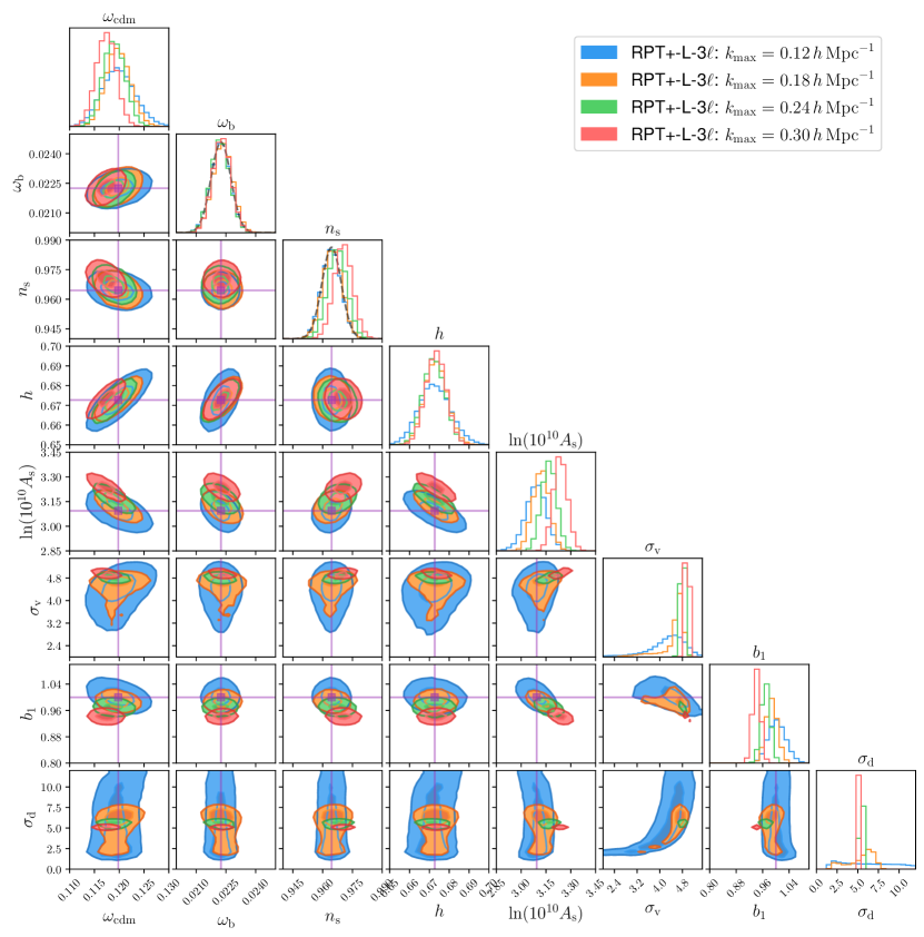
Figure 12: Same as Figure 11 but for RegPT+ with Lorentzian FoG and 3 multipoles. The unit of $\sigma_{\mathrm{v}}$ and $\sigma_{\mathrm{d}}$ is $h^{-1}\,\mathrm{Mpc}$.

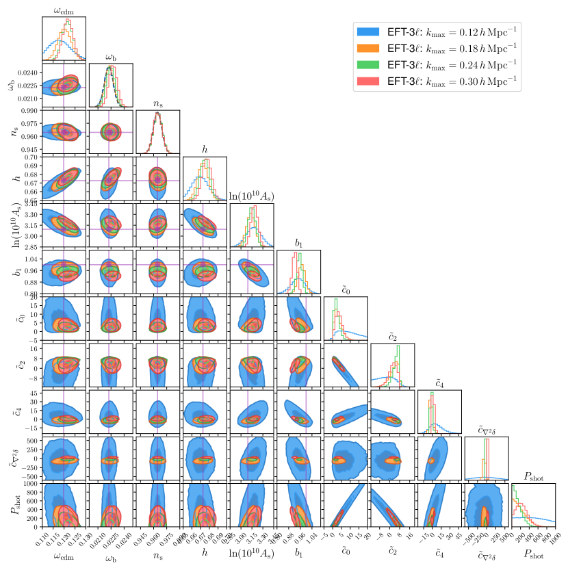
Figure 13: Same as Figure 11 but for IR-resummed EFT with 3 multipoles. The unit of $P_{\mathrm{shot}}$ is $(h^{-1}\,\mathrm{Mpc})^{3}$.

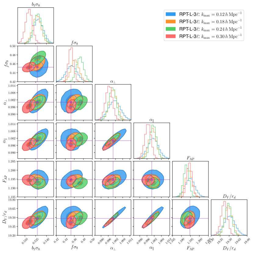
Figure 14: Constraints of derived parameters inferred with RegPT with 3 multipoles. for $k_{\mathrm{max}}=0.12,0.18,0.24,0.30\,h\,\mathrm{Mpc}^{-1}$. The inner and outer ellipses correspond to the $1\text{-}\sigma$ and $2\text{-}\sigma$ confidence levels, respectively. The purple lines correspond to fiducial values.

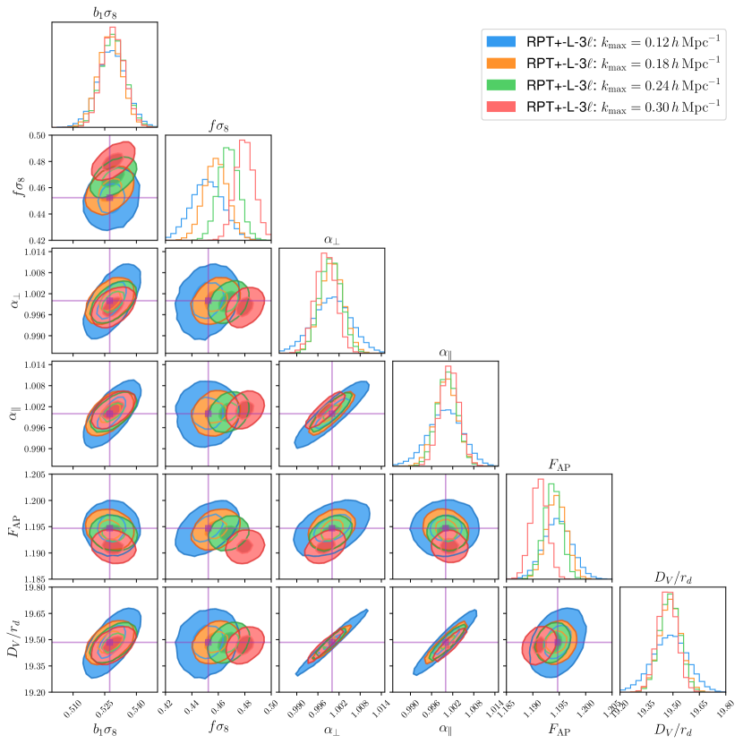
Figure 15: Same as Figure 14 but RegPT+ with Lorentzian FoG and 3 multipoles.

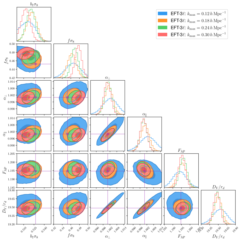
Figure 16: Same as Figure 14 but for IR-resummed EFT with 3 multipoles.

V.3 Figure of Bias, Figure of Merit, and reduced chi-square

Here, we discuss the measures to quantify the parameter bias, the constraining power, and the goodness of fit. First, we compute the covariance matrix of parameters $S$ from the chains:

$$S_{\alpha\beta}=\frac{1}{N-1}\sum_{i=1}^{N}(\theta_{\alpha}^{i}-\bar{\theta}_{\alpha})(\theta_{\beta}^{i}-\bar{\theta}_{\beta}),$$ (67)

where $N$ is the number of samples in the chain and $\bar{\bm{\theta}}$ is the sample mean of the parameter. In order to evaluate the parameter bias, we define Figure of Bias (FoB):

$$\mathrm{FoB}\equiv\left[\sum_{\alpha,\beta}\delta\theta_{\alpha}\left(\tilde{S}\right)^{-1}_{\alpha\beta}\delta\theta_{\beta}\right]^{\frac{1}{2}},$$ (68)

where the covariance matrix $\tilde{S}$ is marginalized over all nuisance parameters from the full parameter covariance matrix $S$ and $\delta\bm{\theta}=\bar{\bm{\theta}}-\bm{\theta}^{\mathrm{fid}}$ is the difference between the sample mean and the fiducial parameter. The probability distribution of FoB is the chi-squared distribution with the degree of freedom of $5$. Then, we define the $1\text{-}\sigma$, $2\text{-}\sigma$, and $3\text{-}\sigma$ critical values of FoB, which are $68\%$, $95\%$, and $99.7\%$ percentiles, respectively.

Next, in order to evaluate the constraining power, we define the Figure of Merit (FoM):

$$\mathrm{FoM}\equiv\frac{V_{\theta}}{\sqrt{\det\tilde{S}}},$$ (69)

where $V_{\theta}=\prod_{\alpha}\theta_{\alpha}^{\mathrm{fid}}$ is the normalization factor and the subscript $\alpha$ runs over five cosmological parameters. The FoM is roughly proportional to the hyper volume of $1\text{-}\sigma$ confidence region and thus, larger FoM implies stronger constraining power.

The measure of the goodness of fit is the reduced chi-square $\chi^{2}/N_{\mathrm{dof}}$, where $\chi^{2}$ is the best-fit chi-square (Eqs. 58 and 60) and $N_{\mathrm{dof}}$ is the effective degree of freedom. We have introduced priors of several parameters and the information content of the priors should be considered in the degree of freedom. The effective number of parameters $N_{\mathrm{eff}}$ is given as [81]

$$N_{\mathrm{eff}}=N_{p}-\mathrm{tr}[\mathcal{C}_{\mathrm{prior}}^{-1}\mathcal{C}],$$ (70)

where $N_{p}$ is the number of parameters (cosmological parameters plus nuisance parameters), and $\mathcal{C}$ and $\mathcal{C}_{\mathrm{prior}}$ is the covariance matrix of posterior and prior parameters, respectively. Since all the adopted priors are Gaussian, the expression of the second term can be simplified as

$$\mathrm{tr}[\mathcal{C}_{\mathrm{prior}}^{-1}\mathcal{C}]=\sum_{\alpha}\frac{\hat{\sigma}^{2}_{\alpha}}{\sigma^{2}_{\alpha}},$$ (71)

where the summation runs over parameters with priors ($\alpha=\omega_{\mathrm{b}},n_{\mathrm{s}}$), $\hat{\sigma}^{2}_{\theta}$ is the sample variance of the parameter computed from the chain, and $\sigma^{2}_{\theta}$ is the variance of the prior. As a result, the degree of freedom is given as

$$N_{\mathrm{dof}}=N_{\mathrm{data}}-N_{\mathrm{eff}},$$ (72)

where $N_{\mathrm{data}}$ is the number of data points. Note that the reduced chi-square in this analysis does not follow the chi-square distribution because we have generated the initial condition of the $N$-body simulation with the paired and fixed approach. Therefore, the cosmic variance is strongly suppressed and the reduced chi-square is always close to zero.

In order to highlight the difference between models, we discuss the results for following groups:

Group A

RegPT and RegPT+ with Lorentzian FoG with and without AP effect, and IR-resummed EFT with 3 multipoles,

Group B

RegPT and RegPT+ with Gaussian FoG, $\gamma$ FoG, and IR-resummed EFT with 3 multipoles,

Group C

RegPT and RegPT+ with Lorentzian, Gaussian, $\gamma$ FoGs with 3 multipoles,

Group D

RegPT with 3/2 multipoles and 3/2 wedges,

Group E

RegPT+ with 3/2 multipoles and 3/2 wedges,

Group F

IR-resummed EFT with 3/2 multipoles and 3/2 wedges.

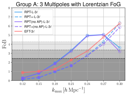
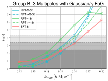
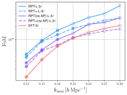
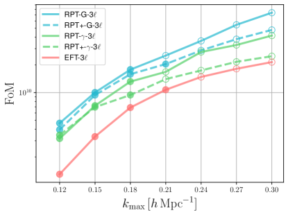
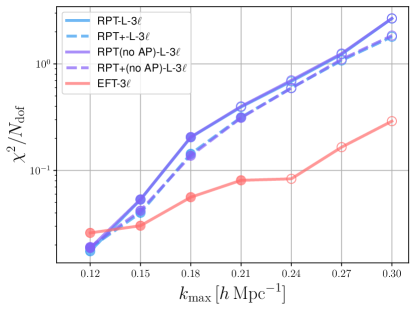
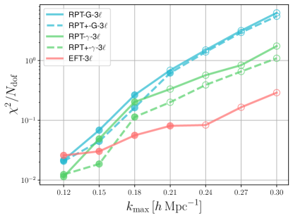
Figure 17: The FoB (upper panels), FoM (middle panels), and reduced chi-square (lower panels) for Group A (left panels) and Group B (right panels). For FoB, the gray regions correspond to $1\text{-}\sigma$, $2\text{-}\sigma$, and $3\text{-}\sigma$ critical values from bottom to top.

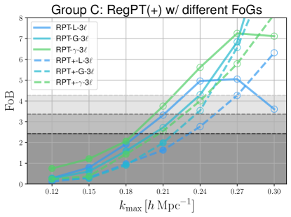
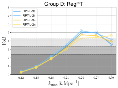
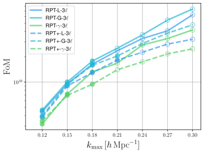
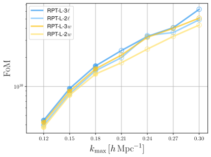
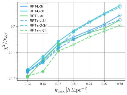
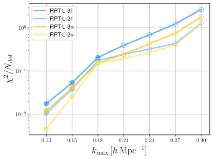
Figure 18: Same as Figure 17 but for Group C (left panels) and Group D (right panels).

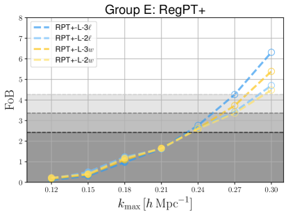
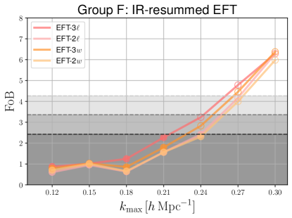
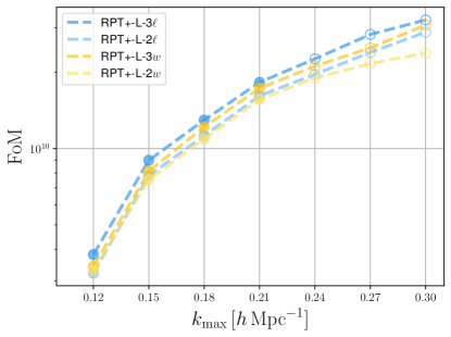
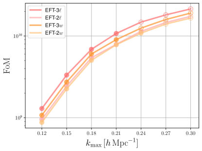
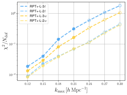
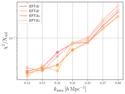
Figure 19: Same as Figure 17 but for Group E (left panels) and Group F (right panels).

Figures 17, 18, and 19 show the FoB, FoM, and reduced chi-square for each group.

V.3.1 Group A

This group consists of RegPT, RegPT+, and IR-resummed EFT with the 3 multipoles data vector. First, FoBs of RegPT+ are the lowest among the models presented and they do not exceed the $1\text{-}\sigma$ critical value up to $k_{\mathrm{max}}=0.21\,h\,\mathrm{Mpc}^{-1}$ whereas FoB for RegPT with $k_{\mathrm{max}}=0.21\,h\,\mathrm{Mpc}^{-1}$ is around the $2\text{-}\sigma$ level. In terms of FoM, the FoM of RegPT is always the highest because RegPT contains only two nuisance parameters (three for RegPT+), which can be degenerate with cosmological parameters and as a result, weaken parameter constraints. However, the highest FoM with unbiased parameter estimates, i.e. FoB less than the $1\text{-}\sigma$ value, can be achieved by RegPT+ though there is only a slight difference between RegPT and RegPT+. Second, FoB of IR-resummed EFT is comparable with RegPT+ but FoM is much smaller than RegPT and RegPT+ because the number of nuisance parameters of IR-resummed EFT is six and these many nuisance parameters lead to weak parameter constraints. On the other hand, reduced chi-squares of IR-resummed EFT are the smallest except $k_{\mathrm{max}}=0.12\,h\,\mathrm{Mpc}^{-1}$. This feature has an important implication that the good fit to the measured power spectrum does not guarantee the tight or unbiased parameter constraints and potentially, over-fitting occurs due to the large degrees of freedom. Finally, FoB and reduced chi-squares are not much affected by the AP effect but FoM with the AP effect considered is higher than that without the AP effect. The AP effect induces additional dependence on cosmological parameters relevant to the geometry, and thus, more information can be accessible from the AP effect. Therefore, when the AP effect is considered, the parameter constraints become tighter and the resultant FoM becomes larger.

V.3.2 Group B

In this group, we investigate whether the performance of RegPT and RegPT+ in comparison with IR-resummed EFT, which is addressed in Group A, is affected by different FoG functional forms: Gaussian and $\gamma$ FoGs. The general trend is quite similar to the results with fiducial Lorentzian FoG; though the reduced chi-square is larger compared with IR-resummed EFT, FoM and FoB for both models with Gaussian or $\gamma$ FoG are better. That is because these models contain less nuisance parameters.

V.3.3 Group C

Here, we address how the choice of functional form of FoG function affects the measures. The $\gamma$ FoG has one additional free parameter which determines the shape of the FoG function and includes Loretzian and Gaussian forms as a special case. The best-performing model in terms of FoB and FoM is Gaussian for RegPT and RegPT+. Though the fitting results for hexadecapole moments with Gaussian FoGs are worse than Lorentzian FoG, the models with Gaussian FoG can perform better for monopole and quadrupole moments. The reduced chi-square with the $\gamma$ FoG is the best compared with other FoG models. However, the FoM and FoB are significantly worse and thus, the free parameter of the $\gamma$ FoG leads to over-fitting to the data.

V.3.4 Group D

This group addresses the choice of data vectors with RegPT: 3/2 multipoles and 3/2 wedges. The 3 (2) multipoles and 3 (2) wedges contain the same number of data points but different projection of the anisotropic power spectrum is adopted. For FoB, the results for the pair of results of 3 (2) multipoles and 3 (2) wedges are quite similar. On the other hand, FoM is better for multipoles and reduced chi-square is smaller for wedges. Originally, the concept of wedges has been proposed in Ref. [62] to efficiently constrain the geometry of the Universe. The transverse wedge ($0<\mu<1/2$) and radial wedge ($1/2<\mu<1$) are sensitive to $H(z)$ and $D_{A}(z)$, respectively. However, our analysis incorporates the full shape information of the power spectrum, and in this case, the multipole expansion can constrain parameters better because it weights the anisotropic part of the power spectrum more. We have investigated only the equally spaced wedges but the different spacing of wedges, e.g. weighing more on $\mu\simeq 0$ to avoid the region where FoG damping is eminent, has the potential to yield performance similar to multipoles.

V.3.5 Group E

This group presents results similar to those in Group D but with RegPT+. For FoB, the results are almost the same as Group D but the difference for FoM and chi-square is clearer. The RegPT+ has better flexibility of the FoG damping and thus, can extract more information from the power spectrum at directions where strong FoG damping happens, i.e., $\mu\simeq 1$.

V.3.6 Group F

This group also presents results for different data vectors with IR-resummed EFT. The general trend is the same as Group D and Group E but the difference due to data vectors is comparable with RegPT but less significant than RegPT+. Note that for all data vectors the reduced chi-squares are the lowest among all PT models but in compensation, FoMs are the lowest and thus, the constraining power of cosmological parameters is weak. It should be noted that the reduced chi-square with small $k_{\mathrm{max}}$ is unstable because there are too many free parameters compared with the number of data points and over-fitting may occur in this case.

To summarize, Figure 20 illustrates the highest FoM achieved by each model with the constraint that FoB does not exceed the $1\text{-}\sigma$ critical value. RegPT+ generally performs better than RegPT and the best-performing model among all the examined models is RegPT+ with Gaussian FoG and 3 multipoles. IR-resummed EFT with 2 multipoles or 2 wedges can utilize the small-scale power spectra up to $k_{\mathrm{max}}=0.24\,h\,\mathrm{Mpc}^{-1}$. However, due to many nuisance parameters introduced in IR-resummed EFT, the parameter constraining power, i.e. FoM, is weaker than RegPT and RegPT+. There is a caveat about IR-resummed EFT. In the presented results, the order of IR-resummed EFT is 1-loop in contrast to 2-loop for RegPT and RegPT+ since the implementation of IR-resummed EFT at the 2-loop order is still challenging. Thus, the comparison between 1-loop IR-resummed EFT and 2-loop RegPT and RegPT+ is not fair and IR-resummed EFT at the 2-loop order has potential to achieve the lower FoB with higher $k_{\mathrm{max}}$ than RegPT+.

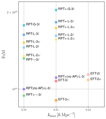
Figure 20: The highest FoM with the constraint that FoB does not exceed the $1\text{-}\sigma$ critical value. RegPT+ with Gaussian FoG and 3 multipoles yields the highest FoM, which is displayed as a star symbol. Note that IR-resummed EFT is at 1-loop order and the FoMs of IR-resummed EFT are shown as square symbols. For reference, a factor of 2 better FoM corresponds to $14.8\%$ better constraint for each parameter on average.

VI Conclusions

The galaxy clustering analysis has been playing a central role in observational cosmology to constrain cosmological parameters. The theoretical model to predict the statistics, e.g., power spectra, given a cosmological model is an essential ingredient in cosmological parameter inference, and the accuracy of the model is critical to place stringent constraints on cosmological parameters. For accurate predictions on small scales, the non-linearity due to gravitational evolution must be incorporated into the model. In addition, the peculiar motion of galaxies distorts the distance estimate in the line-of-sight direction, which is referred to as the RSD effect, and the effect needs to be considered in the theoretical model. A variety of theoretical models based on PT have been proposed and different assumptions are employed depending on the model.

The PT challenge analysis proposed here follows our precedent work [26], where the real space power spectrum is employed. In this work, we extend the PT challenge analysis with the redshift space power spectrum. This was made possible with the help of the implementation of the response function method [46] to accelerate the PT calculations of power spectra with RSD effects and the calculation module is integrated into the framework of Eclairs [59]. In the challenge analysis, we first perform the $N$-body simulation with fiducial cosmological parameters and measure the power spectrum from the matter density field. Then, we regard the measured power spectrum as a given data vector and carry out parameter inference with the PT models described above. The inferred cosmological parameters can then be directly compared with the fiducial values. We can assess the constraining power and the bias of cosmological parameters as the function of the maximum wave-number scale of data points, which we denote $k_{\mathrm{max}}$. More precisely, $k_{\mathrm{max}}$ is determined with the help of the bias parameter, the Figure of Bias (FoB), defined as the difference between the inferred and fiducial values normalized by the covariance. Parameter inference is then tagged as “biased”, and therefore excluded, if FoB exceeds the $1\text{-}\sigma$ critical value as the probability distribution of FoB follows the multi-variate Gaussian distribution. The constraining power of the parameters is defined with a Figure of Merit (FoM), which is the inverse of the square root of the parameter covariance matrix, which corresponds to the inverse of the hyper-volume of confidence regions. The key objective of the PT challenge analysis is then first, for each model to assign a $k_{\mathrm{max}}$ for which its FoB remains below the $1\text{-}\sigma$ critical value, and then to identify the models which yield the highest FoM.

The examined PT models are RegPT, RegPT+, and IR-resummed EFT. RegPT is the extended version of SPT by reorganizing the SPT expansion and the accuracy and convergence have been enhanced compared with SPT. The RegPT+ model contains one additional free parameter giving the dispersion of displacement $\sigma_{\mathrm{d}}$ that controls the small-scale damping feature. Previous studies have shown that taking this parameter as a free parameter can significantly improve the model[26]. The last model is IR-resummed EFT, where the small-scale spectra are described by effective counter terms. This class of models can accurately account for the small-scale power spectra but with the introduction of many nuisance parameters. In addition to different theoretical models, we also address how FoG functional forms, the AP effect, and sampling of data vectors (multipoles or wedges) affect the parameter inference. In this analysis, however, we use a simple, perhaps naive, model of linear galaxy bias and assume Poisson noise. In particular, we assume a simple linear scale independent bias, ignoring the possibility that the galaxy bias is likely to have non-trivial scale dependencies [for a review, see 82]. It should be kept in mind that this is likely to be an important limitation on the scope of the analysis we present below. In particular, the performance of the models we consider is likely to be affected differently when additional nuisance parameters are introduced.

It is also to be noted that the reference survey we consider, in terms of volume and number density of galaxies, reproduces the raw characteristics of the Euclid spectroscopic survey. The conclusions we reach are then a priori valid for such a setting only but we do not expect the results to be very sensitive to those assumptions.

In the PT challenge analysis, five cosmological parameters $(\omega_{\mathrm{b}},\omega_{\mathrm{cdm}},h,\ln(10^{10}A_{\mathrm{s}}),n_{\mathrm{s}})$ and the linear bias parameter $b_{1}$ are inferred from the redshift space power spectrum at the redshift $z=1$ assuming the Gaussian covariance matrix with the survey volume and the galaxy number density expected for the Euclid mission. In order to quantify the goodness of fit and the induced parameter bias, we have introduced three measures: FoM, FoB, and reduced chi-squares. The reduced chi-square is irrelevant to the parameter inference but expresses the performance of the fitting of the power spectrum. The findings derived from the PT challenge analysis are summarized below:

• RegPT yields the highest FoM but the largest reduced chi-square. IR-resummed EFT delivers the opposite results: the lowest FoM but the smallest reduced chi-square. RegPT+ is in between. This feature can be explained by the number of nuisance parameters. RegPT has no nuisance parameter, RegPT+ has one, and IR-resummed EFT has five for 3 multipoles case. The nuisance parameters add flexibility especially at small scales, and thus, introducing nuisance parameters improves the fitting at small scales, i.e., smaller reduced chi-square. However, the nuisance parameters are degenerate with cosmological parameters and thus degrade constraints on cosmological parameters, i.e., lower FoM. The trade-off is also observed in the previous analysis of the real-space power spectrum [26].

• Under the condition that the FoB does not exceed the $1\text{-}\sigma$ critical value, the PT model which yields the highest FoM is RegPT+ with $k_{\mathrm{max}}=0.21\,h\,\mathrm{Mpc}^{-1}$. This model has only one free parameter $\sigma_{\mathrm{d}}$, which controls the small-scale damping feature. Therefore, we can conclude that RegPT+ is the most competent without significant parameter bias among the examined PT models.

• We have examined the different functional forms of FoG damping: Lorentzian, Gaussian, $\gamma$ FoGs. The $\gamma$ FoG has one additional parameter, which determines the shape of the damping, and contains Lorentzian and Gaussian forms as special cases. Among the three models, Gaussian FoG yields the best FoM and FoB. On the other hand, for the $\gamma$ FoG, over-fitting occurs due to the free parameter introduced in the model. Hence, the reduced chi-square is the lowest but the FoM and FoB are the worst.

• The redshift space power spectrum has two arguments: the magnitude of wave-number $k$ and the directional cosine $\mu$ in the line-of-sight direction. In the practical analysis, the variable $\mu$ is projected in two different manners: multipoles and wedges. Overall, for 3 multipoles and 3 wedges, FoMs are slightly better than 2 multipoles and 2 wedges, respectively, because there are more data points and more information is accessible. The difference between 3 (2) multipoles and 3 (2) wedges is quite small but overall, multipoles lead to slightly better FoM but worse reduced chi-square.

These conclusions on the relative performances of the models we explore should not however be considered definitive. In particular, as mentioned before, we made simplifying assumption on galaxy bias behavior. The introduction of a more elaborate model is likely to affect the result and the relative performances of the models. This is precisely what we would like to explore in the subsequent paper of this series, exploiting the fact that the computation of higher-order contributions in galaxy bias expansion can also be accelerated with the response function approach.

Appendix A 1-loop SPT power spectrum in the redshift space

There is another formalism to derive the expression of the power spectrum in the redshift space based on SPT through the mapping of coordinates $\bm{s}=\bm{x}+\frac{v_{z}(\bm{x})}{aH}\hat{z}$, where $\bm{s}$ and $\bm{x}$ are the coordinates in the redshift space and the real space, respectively, and $\hat{z}$ is the unit vector along the line-of-sight direction. Thus, one can obtain the expression of the power spectrum in the redshift space [83, 84, 17] and the expression at the 1-loop order can be reorgarnized with TNS correction terms [50]:

$$P^{\mathrm{(S)}}_{\mathrm{SPT}}(k,\mu)= [1-(k\mu f\sigma_{\mathrm{v},\mathrm{L}})^{2}]$$

$$\times[P_{\delta\delta}(k)+2f\mu^{2}P_{\delta\theta}(k)+f^{2}\mu^{4}P_{\theta\theta}(k)]$$

$$+A(k,\mu)+B(k,\mu)+C(k,\mu),$$ (73)

where the velocity dispersion at linear order $\sigma^{2}_{\mathrm{v,L}}$ is defined in Eq. (26). The power spectra $P_{\delta\delta}(k)$, $P_{\delta\theta}(k)$, and $P_{\theta\theta}(k)$ are computed based on SPT at 1-loop order. For the correction terms at the 1-loop order, the bispectra in the $A$-term and the power spectra in the $B$-term should be computed at the tree level, i.e., $P_{ab}(k,z)=P_{\mathrm{L}}(k,z)$. Then, the $C$-term is given as

$$C(k,\mu)= (k\mu f)^{2}\int\frac{\differential[3]p}{(2\pi)^{3}}\frac{\differential[3]q}{(2\pi)^{3}}\delta_{\mathrm{D}}(\bm{k}-\bm{p}-\bm{q})\frac{\mu_{p}^{2}}{p^{2}}P_{\theta\theta}(p)$$

$$\times\left\{P_{\delta\delta}(q)+2f\mu_{q}^{2}P_{\delta\theta}(q)+f^{2}\mu_{q}^{4}P_{\theta\theta}(q)\right\},$$ (74)

where $\mu_{p}=p_{z}/p$ and $\mu_{q}=q_{z}/q$. To keep the consistency of the order, the power spectra should be computed at the linear order. Then, the $C$-term is given as

$$C(k,\mu)= \sum_{n=1}^{3}\sum_{a,b=1}^{2}\mu^{2n}(-f)^{a+b}\frac{k^{3}}{(2\pi)^{2}}\int_{0}^{\infty}\!\!\differential r\int_{-1}^{+1}\!\!\differential x$$

$$\times\left[C^{n}_{ab}(r,x)P_{ab}\left(k\sqrt{1+r^{2}-2rx}\right)P_{22}(kr)\right.$$

$$\left.+\tilde{C}^{n}_{ab}(r,x)P_{22}\left(k\sqrt{1+r^{2}-2rx}\right)P_{ab}(kr)\right].$$ (75)

The non-vanishing components of $C^{n}_{ab}(r,x)$ and $\tilde{C}^{n}_{ab}(r,x)$ are

$$C^{1}_{11}(r,x)= -\frac{x^{2}-1}{4},$$ (76)

$$C^{1}_{12}(r,x)= -\frac{3r^{2}(x^{2}-1)^{2}}{8(1+r^{2}-2rx)},$$ (77)

$$C^{1}_{22}(r,x)= -\frac{5r^{4}(x^{2}-1)^{3}}{16(1+r^{2}-2rx)^{2}},$$ (78)

$$C^{2}_{11}(r,x)= \frac{3x^{2}-1}{4},$$ (79)

$$C^{2}_{12}(r,x)= \frac{(x^{2}-1)(2-12rx-3r^{2}+15r^{2}x^{2})}{4(1+r^{2}-2rx)},$$ (80)

$$C^{2}_{22}(r,x)= \frac{3r^{2}(x^{2}-1)^{2}(7-30rx-5r^{2}+35r^{2}x^{2})}{16(1+r^{2}-2rx)^{2}},$$ (81)

$$C^{3}_{12}(r,x)= -\frac{-4+12x^{2}+8rx(3-5x^{2})+r^{2}(3-30x^{2}+35x^{4})}{8(1+r^{2}-2rx)},$$ (82)

$$C^{3}_{22}(r,x)= -\frac{(x^{2}-1)[4+3r\{-16x+r(-14+70x^{2}+20rx(3-7x^{2})+5r^{2}(1-14x^{2}+21x^{4}))\}]}{16(1+r^{2}-2rx)^{2}},$$ (83)

$$C^{4}_{22}(r,x)= \frac{-4+12x^{2}+16rx(3-5x^{2})+7r^{2}(3-30x^{2}+35x^{4})-6r^{3}x(15-70x^{2}+63x^{4})}{16(1+r^{2}-2rx)^{2}}$$

$$+\frac{r^{4}\{-5+21x^{2}(5-15x^{2}+11x^{4})\}}{16(1+r^{2}-2rx)^{2}},$$ (84)

$$\tilde{C}^{1}_{11}(r,x)= -\frac{r^{4}(x^{2}-1)}{4(1+r^{2}-2rx)^{2}},$$ (85)

$$\tilde{C}^{1}_{12}(r,x)= -\frac{3r^{4}(x^{2}-1)}{8(1+r^{2}-2rx)^{2}},$$ (86)

$$\tilde{C}^{2}_{11}(r,x)= \frac{r^{2}(2-4rx-r^{2}+3r^{2}x^{2})}{4(1+r^{2}-2rx)^{2}},$$ (87)

$$\tilde{C}^{2}_{12}(r,x)= \frac{r^{2}(x^{2}-1)(2-12rx-3r^{2}+15r^{2}x^{2})}{4(1+r^{2}-2rx)^{2}},$$ (88)

$$\tilde{C}^{3}_{12}(r,x)= -\frac{r^{2}\{-4+12x^{2}+8rx(3-5x^{2})+r^{2}(3-30x^{2}+35x^{4})\}}{8(1+r^{2}-2rx)^{2}}.$$ (89)

The scaling of $C$-terms with respect to the linear bias $b_{1}$ is given as

$$C(k,\mu;f)\to b_{1}^{4}C(k,\mu;\beta).$$ (90)

Appendix B PT Challenge results with models at the 1-loop order

Here, we carry out the PT challenge analysis for SPT, RegPT, and RegPT+ at the 1-loop order to investigate the effect of the order of PT models. For these 1-loop PT models, the computational cost is not problematic and thus, we use the direct integration for computations instead of the response function approach. Table 3 summarizes the examined models and we define Group G, which includes RegPT and RegPT+ at the 1-loop and 2-loop orders and SPT and IR-resummed EFT at the 1-loop order to investigate measures of FoB, FoM, and the reduced chi-square. In this group, the FoG damping function and the data vector are fixed as Lorentzian and 3 multipoles, respectively, and the AP effect is included. First, SPT demonstrates poor performance even at the small $k_{\mathrm{max}}$. The FoB is already larger than the $1\text{-}\sigma$ critical value at $k_{\mathrm{max}}=0.12\,h\,\mathrm{Mpc}^{-1}$. As SPT has no nuisance parameters, it yields high FoM. However, the FoB and reduced chi-square are too high and thus, SPT at the 1-loop order cannot be used to robustly constrain cosmological parameters. In terms of RegPT, FoB is better for the 2-loop model and FoB of the 1-loop model suddenly increases at $k_{\mathrm{max}}=0.21\,h\,\mathrm{Mpc}^{-1}$ because the accuracy at the small scale of this model is worse. A similar feature is found in the reduced chi-square. The FoM is quite similar at lower $k_{\mathrm{max}}$ because the number of the nuisance parameter is the same. In contrast, the performance of RegPT and RegPT+ is comparable but FoM is better for the 2-loop PT model. The free parameter specific to RegPT+, i.e., the dispersion of displacement, has considerable flexibility to fit the small-scale power spectrum. IR-resummed EFT yields the lowest reduced chi-square and FoM is slightly higher than RegPT+. Similarly to the 2-loop case, FoM of IR-resummed EFT is quite suppressed due to many nuisance parameters.

Table 3: Descriptions of models with RegPT, RegPT+, and SPT at the 1-loop order.

Label	PT Model	Data vector	AP	FoG	Nuisance parameters
RPT(1-loop)-L-3$\ell$	RegPT	3 Multipoles ($\ell=0,2,4$)	✓	Lorentzian	$b_{1},\sigma_{\mathrm{v}}$
RPT+(1-loop)-L-3$\ell$	RegPT+	3 Multipoles ($\ell=0,2,4$)	✓	Lorentzian	$b_{1},\sigma_{\mathrm{v}},\sigma_{\mathrm{d}}$
SPT(1-loop)-3$\ell$	SPT	3 Multipoles ($\ell=0,2,4$)	✓	—	$b_{1}$

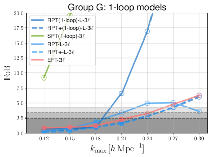
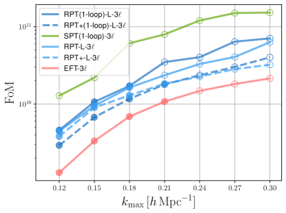
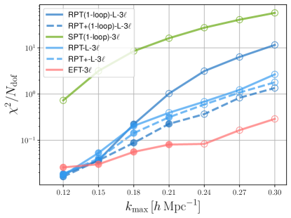
Figure 21: The FoB (upper panels), FoM (middle panels), and reduced chi-square (lower panels) for Group G.

References

- White and Frenk [1991] S. D. M. White and C. S. Frenk, Astrophys. J. 379, 52 (1991).
- Aubourg et al. [2015] É. Aubourg, S. Bailey, J. E. Bautista, F. Beutler, V. Bhardwaj, D. Bizyaev, M. Blanton, M. Blomqvist, A. S. Bolton, J. Bovy, H. Brewington, J. Brinkmann, J. R. Brownstein, A. Burden, N. G. Busca, W. Carithers, C.-H. Chuang, J. Comparat, R. A. C. Croft, A. J. Cuesta, K. S. Dawson, T. Delubac, D. J. Eisenstein, A. Font-Ribera, J. Ge, J. M. Le Goff, S. G. A. Gontcho, J. R. Gott, J. E. Gunn, H. Guo, J. Guy, J.-C. Hamilton, S. Ho, K. Honscheid, C. Howlett, D. Kirkby, F. S. Kitaura, J.-P. Kneib, K.-G. Lee, D. Long, R. H. Lupton, M. V. Magaña, V. Malanushenko, E. Malanushenko, M. Manera, C. Maraston, D. Margala, C. K. McBride, J. Miralda-Escudé, A. D. Myers, R. C. Nichol, P. Noterdaeme, S. E. Nuza, M. D. Olmstead, D. Oravetz, I. Pâris, N. Padmanabhan, N. Palanque-Delabrouille, K. Pan, M. Pellejero-Ibanez, W. J. Percival, P. Petitjean, M. M. Pieri, F. Prada, B. Reid, J. Rich, N. A. Roe, A. J. Ross, N. P. Ross, G. Rossi, J. A. Rubiño-Martín, A. G. Sánchez, L. Samushia, R. T. Génova-Santos, C. G. Scóccola, D. J. Schlegel, D. P. Schneider, H.-J. Seo, E. Sheldon, A. Simmons, R. A. Skibba, A. Slosar, M. A. Strauss, D. Thomas, J. L. Tinker, R. Tojeiro, J. A. Vazquez, M. Viel, D. A. Wake, B. A. Weaver, D. H. Weinberg, W. M. Wood-Vasey, C. Yèche, I. Zehavi, G.-B. Zhao, and BOSS Collaboration, Phys. Rev. D 92, 123516 (2015), arXiv:1411.1074 [astro-ph.CO] .
- Weinberg et al. [2013] D. H. Weinberg, M. J. Mortonson, D. J. Eisenstein, C. Hirata, A. G. Riess, and E. Rozo, Phys. Rept. 530, 87 (2013), arXiv:1201.2434 [astro-ph.CO] .
- Beutler et al. [2011] F. Beutler, C. Blake, M. Colless, D. H. Jones, L. Staveley-Smith, L. Campbell, Q. Parker, W. Saunders, and F. Watson, Mon. Not. Roy. Astron. Soc. 416, 3017 (2011), arXiv:1106.3366 [astro-ph.CO] .
- Blake et al. [2011] C. Blake, E. A. Kazin, F. Beutler, T. M. Davis, D. Parkinson, S. Brough, M. Colless, C. Contreras, W. Couch, S. Croom, D. Croton, M. J. Drinkwater, K. Forster, D. Gilbank, M. Gladders, K. Glazebrook, B. Jelliffe, R. J. Jurek, I. H. Li, B. Madore, D. C. Martin, K. Pimbblet, G. B. Poole, M. Pracy, R. Sharp, E. Wisnioski, D. Woods, T. K. Wyder, and H. K. C. Yee, Mon. Not. Roy. Astron. Soc. 418, 1707 (2011), arXiv:1108.2635 [astro-ph.CO] .
- de la Torre et al. [2017] S. de la Torre, E. Jullo, C. Giocoli, A. Pezzotta, J. Bel, B. R. Granett, L. Guzzo, B. Garilli, M. Scodeggio, M. Bolzonella, U. Abbas, C. Adami, D. Bottini, A. Cappi, O. Cucciati, I. Davidzon, P. Franzetti, A. Fritz, A. Iovino, J. Krywult, V. Le Brun, O. Le Fèvre, D. Maccagni, K. Małek, F. Marulli, M. Polletta, A. Pollo, L. A. M. Tasca, R. Tojeiro, D. Vergani, A. Zanichelli, S. Arnouts, E. Branchini, J. Coupon, G. De Lucia, O. Ilbert, T. Moutard, L. Moscardini, J. A. Peacock, R. B. Metcalf, F. Prada, and G. Yepes, Astron. Astrophys. 608, A44 (2017), arXiv:1612.05647 [astro-ph.CO] .
- Alam et al. [2021] S. Alam, M. Aubert, S. Avila, C. Balland, J. E. Bautista, M. A. Bershady, D. Bizyaev, M. R. Blanton, A. S. Bolton, J. Bovy, J. Brinkmann, J. R. Brownstein, E. Burtin, S. Chabanier, M. J. Chapman, P. D. Choi, C.-H. Chuang, J. Comparat, M.-C. Cousinou, A. Cuceu, K. S. Dawson, S. de la Torre, A. de Mattia, V. d. S. Agathe, H. d. M. des Bourboux, S. Escoffier, T. Etourneau, J. Farr, A. Font-Ribera, P. M. Frinchaboy, S. Fromenteau, H. Gil-Marín, J.-M. Le Goff, A. X. Gonzalez-Morales, V. Gonzalez-Perez, K. Grabowski, J. Guy, A. J. Hawken, J. Hou, H. Kong, J. Parker, M. Klaene, J.-P. Kneib, S. Lin, D. Long, B. W. Lyke, A. de la Macorra, P. Martini, K. Masters, F. G. Mohammad, J. Moon, E.-M. Mueller, A. Muñoz-Gutiérrez, A. D. Myers, S. Nadathur, R. Neveux, J. A. Newman, P. Noterdaeme, A. Oravetz, D. Oravetz, N. Palanque-Delabrouille, K. Pan, R. Paviot, W. J. Percival, I. Pérez-Ràfols, P. Petitjean, M. M. Pieri, A. Prakash, A. Raichoor, C. Ravoux, M. Rezaie, J. Rich, A. J. Ross, G. Rossi, R. Ruggeri, V. Ruhlmann-Kleider, A. G. Sánchez, F. J. Sánchez, J. R. Sánchez-Gallego, C. Sayres, D. P. Schneider, H.-J. Seo, A. Shafieloo, A. Slosar, A. Smith, J. Stermer, A. Tamone, J. L. Tinker, R. Tojeiro, M. Vargas-Magaña, A. Variu, Y. Wang, B. A. Weaver, A.-M. Weijmans, C. Yèche, P. Zarrouk, C. Zhao, G.-B. Zhao, and Z. Zheng, Phys. Rev. D 103, 083533 (2021), arXiv:2007.08991 [astro-ph.CO] .
- Takada et al. [2014] M. Takada, R. S. Ellis, M. Chiba, J. E. Greene, H. Aihara, N. Arimoto, K. Bundy, J. Cohen, O. Doré, G. Graves, J. E. Gunn, T. Heckman, C. M. Hirata, P. Ho, J.-P. Kneib, O. Le Fèvre, L. Lin, S. More, H. Murayama, T. Nagao, M. Ouchi, M. Seiffert, J. D. Silverman, L. Sodré, D. N. Spergel, M. A. Strauss, H. Sugai, Y. Suto, H. Takami, and R. Wyse, Publ. Astron. Soc. Jpn. 66, R1 (2014), arXiv:1206.0737 [astro-ph.CO] .
- DESI Collaboration [2016a] DESI Collaboration, arXiv e-prints , arXiv:1611.00036 (2016a), arXiv:1611.00036 [astro-ph.IM] .
- DESI Collaboration [2016b] DESI Collaboration, arXiv e-prints , arXiv:1611.00037 (2016b), arXiv:1611.00037 [astro-ph.IM] .
- Laureijs et al. [2011] R. Laureijs, J. Amiaux, S. Arduini, J. L. Auguères, J. Brinchmann, R. Cole, M. Cropper, C. Dabin, L. Duvet, A. Ealet, B. Garilli, P. Gondoin, L. Guzzo, J. Hoar, H. Hoekstra, R. Holmes, T. Kitching, T. Maciaszek, Y. Mellier, F. Pasian, W. Percival, J. Rhodes, G. Saavedra Criado, M. Sauvage, R. Scaramella, L. Valenziano, S. Warren, R. Bender, F. Castander, A. Cimatti, O. Le Fèvre, H. Kurki-Suonio, M. Levi, P. Lilje, G. Meylan, R. Nichol, K. Pedersen, V. Popa, R. Rebolo Lopez, H. W. Rix, H. Rottgering, W. Zeilinger, F. Grupp, P. Hudelot, R. Massey, M. Meneghetti, L. Miller, S. Paltani, S. Paulin-Henriksson, S. Pires, C. Saxton, T. Schrabback, G. Seidel, J. Walsh, N. Aghanim, L. Amendola, J. Bartlett, C. Baccigalupi, J. P. Beaulieu, K. Benabed, J. G. Cuby, D. Elbaz, P. Fosalba, G. Gavazzi, A. Helmi, I. Hook, M. Irwin, J. P. Kneib, M. Kunz, F. Mannucci, L. Moscardini, C. Tao, R. Teyssier, J. Weller, G. Zamorani, M. R. Zapatero Osorio, O. Boulade, J. J. Foumond, A. Di Giorgio, P. Guttridge, A. James, M. Kemp, J. Martignac, A. Spencer, D. Walton, T. Blümchen, C. Bonoli, F. Bortoletto, C. Cerna, L. Corcione, C. Fabron, K. Jahnke, S. Ligori, F. Madrid, L. Martin, G. Morgante, T. Pamplona, E. Prieto, M. Riva, R. Toledo, M. Trifoglio, F. Zerbi, F. Abdalla, M. Douspis, C. Grenet, S. Borgani, R. Bouwens, F. Courbin, J. M. Delouis, P. Dubath, A. Fontana, M. Frailis, A. Grazian, J. Koppenhöfer, O. Mansutti, M. Melchior, M. Mignoli, J. Mohr, C. Neissner, K. Noddle, M. Poncet, M. Scodeggio, S. Serrano, N. Shane, J. L. Starck, C. Surace, A. Taylor, G. Verdoes-Kleijn, C. Vuerli, O. R. Williams, A. Zacchei, B. Altieri, I. Escudero Sanz, R. Kohley, T. Oosterbroek, P. Astier, D. Bacon, S. Bardelli, C. Baugh, F. Bellagamba, C. Benoist, D. Bianchi, A. Biviano, E. Branchini, C. Carbone, V. Cardone, D. Clements, S. Colombi, C. Conselice, G. Cresci, N. Deacon, J. Dunlop, C. Fedeli, F. Fontanot, P. Franzetti, C. Giocoli, J. Garcia-Bellido, J. Gow, A. Heavens, P. Hewett, C. Heymans, A. Holland, Z. Huang, O. Ilbert, B. Joachimi, E. Jennins, E. Kerins, A. Kiessling, D. Kirk, R. Kotak, O. Krause, O. Lahav, F. van Leeuwen, J. Lesgourgues, M. Lombardi, M. Magliocchetti, K. Maguire, E. Majerotto, R. Maoli, F. Marulli, S. Maurogordato, H. McCracken, R. McLure, A. Melchiorri, A. Merson, M. Moresco, M. Nonino, P. Norberg, J. Peacock, R. Pello, M. Penny, V. Pettorino, C. Di Porto, L. Pozzetti, C. Quercellini, M. Radovich, A. Rassat, N. Roche, S. Ronayette, E. Rossetti, B. Sartoris, P. Schneider, E. Semboloni, S. Serjeant, F. Simpson, C. Skordis, G. Smadja, S. Smartt, P. Spano, S. Spiro, M. Sullivan, A. Tilquin, R. Trotta, L. Verde, Y. Wang, G. Williger, G. Zhao, J. Zoubian, and E. Zucca, arXiv e-prints , arXiv:1110.3193 (2011), arXiv:1110.3193 [astro-ph.CO] .
- Amendola et al. [2018] L. Amendola, S. Appleby, A. Avgoustidis, D. Bacon, T. Baker, M. Baldi, N. Bartolo, A. Blanchard, C. Bonvin, S. Borgani, E. Branchini, C. Burrage, S. Camera, C. Carbone, L. Casarini, M. Cropper, C. de Rham, J. P. Dietrich, C. Di Porto, R. Durrer, A. Ealet, P. G. Ferreira, F. Finelli, J. García-Bellido, T. Giannantonio, L. Guzzo, A. Heavens, L. Heisenberg, C. Heymans, H. Hoekstra, L. Hollenstein, R. Holmes, Z. Hwang, K. Jahnke, T. D. Kitching, T. Koivisto, M. Kunz, G. La Vacca, E. Linder, M. March, V. Marra, C. Martins, E. Majerotto, D. Markovic, D. Marsh, F. Marulli, R. Massey, Y. Mellier, F. Montanari, D. F. Mota, N. J. Nunes, W. Percival, V. Pettorino, C. Porciani, C. Quercellini, J. Read, M. Rinaldi, D. Sapone, I. Sawicki, R. Scaramella, C. Skordis, F. Simpson, A. Taylor, S. Thomas, R. Trotta, L. Verde, F. Vernizzi, A. Vollmer, Y. Wang, J. Weller, and T. Zlosnik, Living Reviews in Relativity 21, 2 (2018), arXiv:1606.00180 [astro-ph.CO] .
- Note [1] https://roman.gsfc.nasa.gov/.
- Bernardeau et al. [2002] F. Bernardeau, S. Colombi, E. Gaztañaga, and R. Scoccimarro, Phys. Rept. 367, 1 (2002), arXiv:astro-ph/0112551 [astro-ph] .
- Blas et al. [2014] D. Blas, M. Garny, and T. Konstandin, J. Cosmol. Astropart. Phys. 2014, 010 (2014), arXiv:1309.3308 [astro-ph.CO] .
- Bernardeau et al. [2014] F. Bernardeau, A. Taruya, and T. Nishimichi, Phys. Rev. D 89, 023502 (2014), arXiv:1211.1571 [astro-ph.CO] .
- Matsubara [2008] T. Matsubara, Phys. Rev. D 77, 063530 (2008), arXiv:0711.2521 [astro-ph] .
- Crocce and Scoccimarro [2006] M. Crocce and R. Scoccimarro, Phys. Rev. D 73, 063519 (2006), arXiv:astro-ph/0509418 [astro-ph] .
- Bernardeau et al. [2008] F. Bernardeau, M. Crocce, and R. Scoccimarro, Phys. Rev. D 78, 103521 (2008), arXiv:0806.2334 [astro-ph] .
- Bernardeau et al. [2012] F. Bernardeau, M. Crocce, and R. Scoccimarro, Phys. Rev. D 85, 123519 (2012), arXiv:1112.3895 [astro-ph.CO] .
- Baumann et al. [2012] D. Baumann, A. Nicolis, L. Senatore, and M. Zaldarriaga, J. Cosmol. Astropart. Phys. 2012, 051 (2012), arXiv:1004.2488 [astro-ph.CO] .
- Carrasco et al. [2012] J. J. M. Carrasco, M. P. Hertzberg, and L. Senatore, Journal of High Energy Physics 2012, 82 (2012), arXiv:1206.2926 [astro-ph.CO] .
- Carrasco et al. [2014] J. J. M. Carrasco, S. Foreman, D. Green, and L. Senatore, J. Cosmol. Astropart. Phys. 2014, 057 (2014), arXiv:1310.0464 [astro-ph.CO] .
- Jackson [1972] J. C. Jackson, Mon. Not. Roy. Astron. Soc. 156, 1P (1972), arXiv:0810.3908 [astro-ph] .
- Kaiser [1987] N. Kaiser, Mon. Not. Roy. Astron. Soc. 227, 1 (1987).
- Osato et al. [2019] K. Osato, T. Nishimichi, F. Bernardeau, and A. Taruya, Phys. Rev. D 99, 063530 (2019), arXiv:1810.10104 [astro-ph.CO] .
- Schmittfull et al. [2016] M. Schmittfull, Z. Vlah, and P. McDonald, Phys. Rev. D 93, 103528 (2016), arXiv:1603.04405 [astro-ph.CO] .
- Schmittfull and Vlah [2016] M. Schmittfull and Z. Vlah, Phys. Rev. D 94, 103530 (2016), arXiv:1609.00349 [astro-ph.CO] .
- McEwen et al. [2016] J. E. McEwen, X. Fang, C. M. Hirata, and J. A. Blazek, J. Cosmol. Astropart. Phys. 2016, 015 (2016), arXiv:1603.04826 [astro-ph.CO] .
- Fang et al. [2017] X. Fang, J. A. Blazek, J. E. McEwen, and C. M. Hirata, J. Cosmol. Astropart. Phys. 2017, 030 (2017), arXiv:1609.05978 [astro-ph.CO] .
- Hamilton [2000] A. J. S. Hamilton, Mon. Not. Roy. Astron. Soc. 312, 257 (2000), arXiv:astro-ph/9905191 [astro-ph] .
- d’Amico et al. [2020] G. d’Amico, J. Gleyzes, N. Kokron, K. Markovic, L. Senatore, P. Zhang, F. Beutler, and H. Gil-Marín, J. Cosmol. Astropart. Phys. 2020, 005 (2020), arXiv:1909.05271 [astro-ph.CO] .
- Colas et al. [2020] T. Colas, G. d’Amico, L. Senatore, P. Zhang, and F. Beutler, J. Cosmol. Astropart. Phys. 2020, 001 (2020), arXiv:1909.07951 [astro-ph.CO] .
- Ivanov et al. [2020] M. M. Ivanov, M. Simonović, and M. Zaldarriaga, J. Cosmol. Astropart. Phys. 2020, 042 (2020), arXiv:1909.05277 [astro-ph.CO] .
- Heitmann et al. [2010] K. Heitmann, M. White, C. Wagner, S. Habib, and D. Higdon, Astrophys. J. 715, 104 (2010), arXiv:0812.1052 [astro-ph] .
- Heitmann et al. [2009] K. Heitmann, D. Higdon, M. White, S. Habib, B. J. Williams, E. Lawrence, and C. Wagner, Astrophys. J. 705, 156 (2009), arXiv:0902.0429 [astro-ph.CO] .
- Nishimichi et al. [2019] T. Nishimichi, M. Takada, R. Takahashi, K. Osato, M. Shirasaki, T. Oogi, H. Miyatake, M. Oguri, R. Murata, Y. Kobayashi, and N. Yoshida, Astrophys. J. 884, 29 (2019), arXiv:1811.09504 [astro-ph.CO] .
- Euclid Collaboration [2021] Euclid Collaboration, Mon. Not. Roy. Astron. Soc. 505, 2840 (2021), arXiv:2010.11288 [astro-ph.CO] .
- Kobayashi et al. [2020] Y. Kobayashi, T. Nishimichi, M. Takada, R. Takahashi, and K. Osato, Phys. Rev. D 102, 063504 (2020), arXiv:2005.06122 [astro-ph.CO] .
- Kobayashi et al. [2022] Y. Kobayashi, T. Nishimichi, M. Takada, and H. Miyatake, Phys. Rev. D 105, 083517 (2022), arXiv:2110.06969 [astro-ph.CO] .
- Nishimichi et al. [2020] T. Nishimichi, G. D’Amico, M. M. Ivanov, L. Senatore, M. Simonović, M. Takada, M. Zaldarriaga, and P. Zhang, Phys. Rev. D 102, 123541 (2020), arXiv:2003.08277 [astro-ph.CO] .
- Eggemeier et al. [2020] A. Eggemeier, R. Scoccimarro, M. Crocce, A. Pezzotta, and A. G. Sánchez, Phys. Rev. D 102, 103530 (2020), arXiv:2006.09729 [astro-ph.CO] .
- Eggemeier et al. [2021] A. Eggemeier, R. Scoccimarro, R. E. Smith, M. Crocce, A. Pezzotta, and A. G. Sánchez, Phys. Rev. D 103, 123550 (2021), arXiv:2102.06902 [astro-ph.CO] .
- Pezzotta et al. [2021] A. Pezzotta, M. Crocce, A. Eggemeier, A. G. Sánchez, and R. Scoccimarro, Phys. Rev. D 104, 043531 (2021), arXiv:2102.08315 [astro-ph.CO] .
- Taruya et al. [2012] A. Taruya, F. Bernardeau, T. Nishimichi, and S. Codis, Phys. Rev. D 86, 103528 (2012), arXiv:1208.1191 [astro-ph.CO] .
- Osato et al. [2021] K. Osato, T. Nishimichi, A. Taruya, and F. Bernardeau, Phys. Rev. D 104, 103501 (2021), arXiv:2107.04275 [astro-ph.CO] .
- Planck Collaboration [2016] Planck Collaboration, Astron. Astrophys. 594, A13 (2016), arXiv:1502.01589 [astro-ph.CO] .
- Taruya et al. [2013] A. Taruya, T. Nishimichi, and F. Bernardeau, Phys. Rev. D 87, 083509 (2013), arXiv:1301.3624 [astro-ph.CO] .
- Scoccimarro [2004] R. Scoccimarro, Phys. Rev. D 70, 083007 (2004), arXiv:astro-ph/0407214 [astro-ph] .
- Taruya et al. [2010] A. Taruya, T. Nishimichi, and S. Saito, Phys. Rev. D 82, 063522 (2010), arXiv:1006.0699 [astro-ph.CO] .
- Okumura et al. [2012] T. Okumura, U. Seljak, P. McDonald, and V. Desjacques, J. Cosmol. Astropart. Phys. 2012, 010 (2012), arXiv:1109.1609 [astro-ph.CO] .
- Baldauf et al. [2015] T. Baldauf, M. Mirbabayi, M. Simonović, and M. Zaldarriaga, Phys. Rev. D 92, 043514 (2015), arXiv:1504.04366 [astro-ph.CO] .
- Vlah et al. [2016] Z. Vlah, U. Seljak, M. Yat Chu, and Y. Feng, J. Cosmol. Astropart. Phys. 2016, 057 (2016), arXiv:1509.02120 [astro-ph.CO] .
- Blas et al. [2016] D. Blas, M. Garny, M. M. Ivanov, and S. Sibiryakov, J. Cosmol. Astropart. Phys. 2016, 028 (2016), arXiv:1605.02149 [astro-ph.CO] .
- Eisenstein and Hu [1998] D. J. Eisenstein and W. Hu, Astrophys. J. 496, 605 (1998), arXiv:astro-ph/9709112 [astro-ph] .
- Ivanov and Sibiryakov [2018] M. M. Ivanov and S. Sibiryakov, J. Cosmol. Astropart. Phys. 2018, 053 (2018), arXiv:1804.05080 [astro-ph.CO] .
- Alcock and Paczynski [1979] C. Alcock and B. Paczynski, Nature (London) 281, 358 (1979).
- Padmanabhan and White [2008] N. Padmanabhan and M. White, Phys. Rev. D 77, 123540 (2008), arXiv:0804.0799 [astro-ph] .
- Osato et al. [2018] K. Osato, T. Nishimichi, F. Bernardeau, and A. Taruya, Eclairs: Efficient Codes for the LArge scales of the unIveRSe, Astrophysics Source Code Library, record ascl:1810.011 (2018), ascl:1810.011 .
- Note [2] https://github.com/0satoken/Eclairs.
- Zhang et al. [2019] J. Zhang, J. Xu, K. Jia, Y. Yin, and Z. Wang, arXiv e-prints , arXiv:1908.01976 (2019), arXiv:1908.01976 [math.ST] .
- Kazin et al. [2012] E. A. Kazin, A. G. Sánchez, and M. R. Blanton, Mon. Not. Roy. Astron. Soc. 419, 3223 (2012), arXiv:1105.2037 [astro-ph.CO] .
- Nishimichi et al. [2017] T. Nishimichi, F. Bernardeau, and A. Taruya, Phys. Rev. D 96, 123515 (2017), arXiv:1708.08946 [astro-ph.CO] .
- Springel [2005] V. Springel, Mon. Not. Roy. Astron. Soc. 364, 1105 (2005), arXiv:astro-ph/0505010 [astro-ph] .
- Scoccimarro [1998] R. Scoccimarro, Mon. Not. Roy. Astron. Soc. 299, 1097 (1998), arXiv:astro-ph/9711187 [astro-ph] .
- Crocce et al. [2006] M. Crocce, S. Pueblas, and R. Scoccimarro, Mon. Not. Roy. Astron. Soc. 373, 369 (2006), arXiv:astro-ph/0606505 [astro-ph] .
- Nishimichi et al. [2009] T. Nishimichi, A. Shirata, A. Taruya, K. Yahata, S. Saito, Y. Suto, R. Takahashi, N. Yoshida, T. Matsubara, N. Sugiyama, I. Kayo, Y. Jing, and K. Yoshikawa, Publ. Astron. Soc. Jpn. 61, 321 (2009), arXiv:0810.0813 [astro-ph] .
- Valageas and Nishimichi [2011] P. Valageas and T. Nishimichi, Astron. Astrophys. 527, A87 (2011), arXiv:1009.0597 [astro-ph.CO] .
- Lewis et al. [2000] A. Lewis, A. Challinor, and A. Lasenby, Astrophys. J. 538, 473 (2000), arXiv:astro-ph/9911177 [astro-ph] .
- Angulo and Pontzen [2016] R. E. Angulo and A. Pontzen, Mon. Not. Roy. Astron. Soc. 462, L1 (2016), arXiv:1603.05253 [astro-ph.CO] .
- Note [3] We take the -direction as the line-of-sight direction, and thus and .
- Grieb et al. [2016] J. N. Grieb, A. G. Sánchez, S. Salazar-Albornoz, and C. Dalla Vecchia, Mon. Not. Roy. Astron. Soc. 457, 1577 (2016), arXiv:1509.04293 [astro-ph.CO] .
- Hand et al. [2017] N. Hand, Y. Li, Z. Slepian, and U. Seljak, J. Cosmol. Astropart. Phys. 2017, 002 (2017), arXiv:1704.02357 [astro-ph.CO] .
- Foreman-Mackey et al. [2013] D. Foreman-Mackey, D. W. Hogg, D. Lang, and J. Goodman, Publ. Astron. Soc. Pac. 125, 306 (2013), arXiv:1202.3665 [astro-ph.IM] .
- Foreman-Mackey et al. [2019] D. Foreman-Mackey, W. Farr, M. Sinha, A. Archibald, D. Hogg, J. Sanders, J. Zuntz, P. Williams, A. Nelson, M. de Val-Borro, T. Erhardt, I. Pashchenko, and O. Pla, The Journal of Open Source Software 4, 1864 (2019), arXiv:1911.07688 [astro-ph.IM] .
- Cooke et al. [2018] R. J. Cooke, M. Pettini, and C. C. Steidel, Astrophys. J. 855, 102 (2018), arXiv:1710.11129 [astro-ph.CO] .
- Note [4] For cases with RegPT+ with , and parameters converge very slowly due to the parameter degeneracy. We relax the convergence criterion only for and so that the length of chains is 20 times longer than the auto-correlation time. For higher , i.e. , the length of the chains is 50 times longer than the auto-correlation time even for and because the parameter degeneracy is broken due to the small-scale data points. The same problem occurs for FoG and the convergence criterion is also relaxed for . For other nuisance parameters, i.e. , and EFT parameters, we adopt the same convergence criterion as cosmological parameters, i.e. 50 times longer than the auto-correlation time. In the presented analysis, nuisance parameters are always marginalized and the relaxation of the convergence criterion does not have significant impacts on results.
- Note [5] See Supplemental Material at [URL will be inserted by publisher] for bestfit and fiducial spectra with all and parameter constraints of all examined models.
- Note [6] We have confirmed that these parameters are consistent with parameters derived by the optimization algorithm within level.
- Note [7] In contrast to fiducial power spectra, the prior information on and is added in this fitting process.
- Raveri and Hu [2019] M. Raveri and W. Hu, Phys. Rev. D 99, 043506 (2019), arXiv:1806.04649 [astro-ph.CO] .
- Desjacques et al. [2018] V. Desjacques, D. Jeong, and F. Schmidt, Phys. Rept. 733, 1 (2018), arXiv:1611.09787 [astro-ph.CO] .
- Heavens et al. [1998] A. F. Heavens, S. Matarrese, and L. Verde, Mon. Not. Roy. Astron. Soc. 301, 797 (1998), arXiv:astro-ph/9808016 [astro-ph] .
- Scoccimarro et al. [1999] R. Scoccimarro, H. M. P. Couchman, and J. A. Frieman, Astrophys. J. 517, 531 (1999), arXiv:astro-ph/9808305 [astro-ph] .