Safe Deployment for Counterfactual Learning to Rank
with Exposure-Based Risk Minimization

Abstract.

CLTR relies on exposure-based inverse propensity scoring (IPS), a LTR-specific adaptation of IPS to correct for position bias. While IPS can provide unbiased and consistent estimates, it often suffers from high variance. Especially when little click data is available, this variance can cause counterfactual learning to rank (CLTR) to learn sub-optimal ranking behavior. Consequently, existing CLTR methods bring significant risks with them, as naively deploying their models can result in very negative user experiences.

We introduce a novel risk-aware CLTR method with theoretical guarantees for safe deployment. We apply a novel exposure-based concept of risk regularization to IPS estimation for LTR. Our risk regularization penalizes the mismatch between the ranking behavior of a learned model and a given safe model. Thereby, it ensures that learned ranking models stay close to a trusted model, when there is high uncertainty in IPS estimation, which greatly reduces the risks during deployment. Our experimental results demonstrate the efficacy of our proposed method, which is effective at avoiding initial periods of bad performance when little date is available, while also maintaining high performance at convergence. For the CLTR field, our novel exposure-based risk minimization method enables practitioners to adopt CLTR methods in a safer manner that mitigates many of the risks attached to previous methods.

1. Introduction

LTR methods optimize ranking systems so that the resulting ranking behavior maximizes a given ranking metric (Liu, 2009). Traditionally, most learning to rank (LTR) methods applied a supervised learning procedure based on manually-created relevance judgements. However, obtaining such judgements is time-consuming, expensive and does not scale (Chapelle and Chang, 2011; Qin et al., 2010). As an alternative, LTR methods have been developed that rely on clicks, as they are much cheaper to obtain in abundance in the form of user interaction logs (Joachims, 2002).

Despite its low costs, click data is generally strongly affected by different forms of interaction bias. Interactions with rankings often suffer from position bias (Craswell et al., 2008): the position at which an item was shown often affects its click through rate (CTR) more than its relevance. As a result, the clicks observed in interaction logs are often more reflective of where items were displayed during logging than how relevant users find them. Thus, naively using this data for LTR, without corrections, can result in heavily biased models with suboptimal ranking performance (Joachims et al., 2017; Wang et al., 2016).

To mitigate the bias problem in interaction data, the field of CLTR has proposed methods to mitigate bias with unbiased estimation (Joachims et al., 2017). CLTR mainly relies on exposure-based IPS (Oosterhuis et al., 2020; Wang et al., 2018), a LTR specific adaptation of the IPS counterfactual estimation method (Swaminathan and Joachims, 2015; Joachims and Swaminathan, 2016; Horvitz and Thompson, 1952). Standard exposure-IPS weights clicks by the inverse effect of position-bias on the clicked item. This procedure thus gives more weight to clicks on items that are underrepresented due to position-bias, and vice versa. In expectation, this removes the effect of position-bias from the loss that is optimized.

Unsafe CLTR. Despite enabling unbiased optimization, IPS is also known to suffer from high variance (Joachims et al., 2017; Oosterhuis, 2022a). In cases with a lack of click data or with large amounts of noise, high variance can make IPS-based CLTR unreliable and lead to very sub-optimal ranking models (Jagerman et al., 2020; Oosterhuis and de Rijke, 2021b). This problem can be so severe that the learned ranking models can be worse than the model used to log the interaction data. Deploying such a learned model could result in a substantially degraded user experience. In other words, despite the improvements that IPS-based CLTR can bring, it is also an unsafe approach since it may lead to considerable deteriorations.

This (un)safety issue is not unique to IPS-based CLTR. Swaminathan and Joachims (2015) address this issue for contextual bandit problems by applying a generalization bound. Such a bound can provide a high-confidence upper limit on the difference between the true and estimated performance of a bandit policy (Shalev-Shwartz and Ben-David, 2014; Thomas et al., 2015). This allows for safer conservative optimization. For instance, Wu and Wang (2018) introduce a bound based on the divergence between the new policy and the logging policy. This bound avoids policies that stray away from the logging policy, unless there is strong evidence that they are actual improvements. This method might appear to be a great fit for CLTR, but, unfortunately, it is based on action propensities that do not generalize well to the very large action spaces in CLTR. Therefore, there is a need for a conservative generalization bound that is practical and effective in the CLTR setting.

Safe CLTR. To address this gap, we propose an exposure-based counterfactual risk minimization (CRM) method that is specifically designed for safe CLTR. Similar to how exposure-based IPS deals with the large action spaces in ranking settings, our method is based on an exposure-based alternative to action-based generalization bounds. We first introduce a divergence measure based on differences between the distributions of exposure of a new policy and a safe logging policy. Then we provide a novel generalization bound and prove that it is a high-confidence lower-bound on the performance of a learned policy. When uncertain, this bound defaults to preferring the logging policy and thus avoids decreases in performance due to variance. In other words, with high-confidence, ranking models optimized with this bound are guaranteed to never deteriorate the user experience, even when little data is available.

Main contributions. We are the first to address CRM for CLTR and contribute a novel exposure-based CRM method for safe CLTR. Our experimental results show that our proposed method is effective at avoiding initial periods of bad performance when little date is available, while also maintaining high performance at convergence. Our novel exposure-based CRM method thus enables safe CLTR that can mitigate many of risks attached to previous methods. We hope that our contribution makes the adoption of CLTR methods more attractive to practitioners working on real-world search and recommendation systems.

2. Related Work

We review related work on CLTR and CRM in off-policy learning.

2.1. Counterfactual learning to rank

LTR deals with learning optimal rankings to maximize a pre-defined notion of utility (Liu, 2009). Traditionally, LTR systems were optimized using supervised learning on manually-created relevance judgements (Chapelle and Chang, 2011). But the manual curation of relevance judgements is a time-consuming and costly process (Chapelle and Chang, 2011; Qin et al., 2010). Also, manually-graded relevance signals do not always align well with actual user preferences (Sanderson et al., 2010). Due to these shortcomings, LTR from user interactions has become a popular alternative to supervised LTR (Speretta and Gauch, 2005; Jiang et al., 2016; Chapelle and Zhang, 2009; Joachims et al., 2017).

Learning from user interactions/click logs was introduced in the pioneering work of Joachims (2002). Click data is relatively cheap to collect and indicative of actual user preferences (Radlinski et al., 2008). In spite of these advantages, click data is known to be a noisy and biased estimate of the true user preferences (Craswell et al., 2008; Oosterhuis et al., 2020). Some of the common biases identified in the LTR literature are position bias (Craswell et al., 2008): trust bias (Agarwal et al., 2019), and item-selection bias (Oosterhuis and de Rijke, 2020a).

To counter the effect of bias, Joachims et al. (2017) introduced counterfactual learning in the context of LTR. They proposed the application of inverse propensity scoring (IPS), a causal inference technique that has prevalence in the offline bandit learning literature (Joachims and Swaminathan, 2016). IPS models the probability of the user examining a document at a given displayed rank. The inverse of the examination probability, i.e., the inverse propensity, is used to correct for the position bias. As a result of the inverse weighing scheme, IPS-based LTR optimization is unaffected by position bias, in expectation (Joachims et al., 2017). Since its introduction, there has been an increasing interest in the area, with several application of IPS in the context of ranking (Agarwal et al., 2019; Vardasbi et al., 2020; Oosterhuis and de Rijke, 2020a; Wang et al., 2018). Recent work has also explored CLTR under a stochastic logging policy, where some exploration is introduced, as opposed to pure exploitation (Oosterhuis and de Rijke, 2021a, 2020a; Yadav et al., 2021).

With regard to safety in learning from user interactions, Jagerman et al. (2020) introduced the notation of safe exploration for offline contextual bandit algorithms. The authors introduced safe exploration algorithm (SEA), which applies high-confidence performance bounds to safely choose between the deployment of a logging policy and a learned policy. Oosterhuis and de Rijke (2021b) applied this context to LTR and introduced a generalization and specialization framework to safely choose between a generalized feature-based LTR model, and a specialized tabular LTR model. The important difference between prior work and our work is that existing methods safely choose between policies, whereas our method safely optimizes a policy. To the best of our knowledge, we are the first to consider notion of safety for the optimization of LTR models.

2.2. Counterfactual risk minimization for offline learning from logs

A relevant area closely related to CLTR is off-policy learning, or offline learning from bandit feedback data (Joachims and Swaminathan, 2016; Saito and Joachims, 2021; Swaminathan and Joachims, 2015; He et al., 2019). Off-policy learning tries to bridge the mismatch between the action distributions of a new policy and the logging policy (Joachims and Swaminathan, 2016). The most common techniques used to achieve that goal are IPS and importance sampling (Horvitz and Thompson, 1952). However, as noted by Cortes et al. (2010), the IPS estimator can have unbounded variance, which can lead to large errors in its estimation. Consequently, optimization with IPS can result in convergence problems and severely suboptimal policies.

To account for this high-variance problem, Swaminathan and Joachims (2015) introduced counterfactual risk minimization (CRM), an off-policy method that explicitly controls for the variance during off-policy learning from bandit feedback data. Their learning objective consists of both the IPS loss and a variance regularization term, which minimizes the dissimilarity between the two policies. This variance regularization term represents the risk that stems from the variance of the IPS estimation. Computing it requires a pass over the entire data which does not scale well. As a scalable alternative, Wu and Wang (2018) introduced variational counterfactual risk minimization (VCRM), where the authors estimate the risk of the new policy by random sampling from the logged data. The objective function to be optimized in the VCRM method is derived from a generic theoretical analysis of learning from importance sampling (Cortes et al., 2010). The risk term in the VCRM method is defined in terms of a specific divergence between the logging policy and the new policy, known as the Rényi divergence (Rényi, 1961). To the best of our knowledge, there is no work on CRM in a LTR setting, making our work the first to propose a CRM approach for the LTR task.

3. Background

3.1. Learning to rank

The objective of learning to rank methods is to optimize a ranking policy ($\pi$), so that for user-issued queries ($q$) it provides the optimal ranking of their pre-selected candidate document sets ($D_{q}$) (Liu, 2009). Formally, this objective can be expressed as the maximization of the following utility function:

(1) $$U(\pi)=\mathbb{E}_{q}\left[\sum_{d\in D_{q}}\rho(d\mid q,\pi)P(R=1\mid d,q)\right].$$

where $\rho(d\mid q,\pi)$ is the weight $\pi$ gives to document $d$ for query $q$. The choice of $\rho$ determines what metric is optimized, for instance, the well-known normalized discounted cumulative gain (NDCG) metric (Järvelin and Kekäläinen, 2002):

(2) $$\rho_{\text{DCG}}(d\mid q,\pi)=\mathbb{E}_{y\sim\pi(\cdot\mid q)}\left[(\log_{2}(\textrm{rank}(d\mid y)+1))^{-1}\right].$$

where $y$ is a ranking sampled from the policy $\pi$. For this paper, the aim is to optimize the expected number of clicks, the next subsection will explain how we choose $\rho$ accordingly.

3.2. Counterfactual learning to rank

Position bias in clicks. Optimizing the LTR objective in Eq. 1 requires access to the true relevance labels ($P(R=1\mid d,q)$), which is often impossible in real-world ranking settings. As an alternative, CLTR uses clicks, since they are present in abundance as logged user interactions. However, clicks are a biased indicator of relevance; for this paper, we will assume the relation between clicks and relevance is determined by a position-based click model (Joachims et al., 2017; Chuklin et al., 2015). For a document $d$ displayed in ranking $y$ for query $q$, this means the click probability can be decomposed into a rank-based examination probability and a document-based relevance probability:

(3) $$P(C=1\mid d,q,y)=P(E=1\mid\text{rank}(d\mid y))P(R=1\mid d,q).$$

The key characteristic of the position-based click model is that the probability of examination only depends on the rank at which a document is displayed: $P(E=1\mid d,q,y)=P(E=1\mid\text{rank}(d\mid y))$. Furthermore, this model assumes that clicks only take place when a document is both relevant to a user and examined by them. Consequently, the click signal is an indication of both the relevance and examination of documents. Thus, the position at which a document is displayed can have a stronger effect on its click probability than its actual relevance (Craswell et al., 2008).

Inverse-propensity-scoring for CLTR. We assume a setting where $N$ interactions have been logged using the logging policy $\pi_{0}$, for each interaction $i$ the query $q_{i}$, the displayed ranking $y_{i}$, and the clicks $c_{i}$ are logged:

(4) $$\mathcal{D}=\big{\{}q_{i},y_{i},c_{i}\big{\}}^{N}_{i=1}.$$

We will use $c_{i}(d)\in\{0,1\}$ to denote whether document $d$ was clicked at interaction $i$. Furthermore, we choose $\rho$ to match the examination probabilities under $\pi$:

(5) $$\rho(d\mid q,\pi)=\mathbb{E}_{y\sim\pi(\cdot\mid q)}\big{[}P(E=1\mid\text{rank}(d\mid y))\big{]}=\rho(d).$$

Hence, our optimization objective $U(\pi)$ is equal to the expected number of clicks (cf. Eq. 1 and 3).

In order to apply IPS, we need the propensity of each document (Joachims et al., 2017), following Oosterhuis and de Rijke (2021a) we use:

(6) $$\begin{split}\rho(d\mid q,\pi_{0})&=P(E=1\mid\pi_{0},d,q)\\ &=\mathbb{E}_{y\sim\pi_{0}(\cdot\mid q)}\big{[}P(E=1\mid\text{rank}(d\mid y))\big{]}=\rho_{0}(d).\end{split}$$

Thus, the exposure of $d$ represents how likely it is examined when using $\pi_{0}$ for logging. Thereby, it indicates how much the clicks on $d$ underrepresent its relevance. For the sake of brevity, we drop $q$, $\pi$ and $\pi_{0}$ from our notation when their values are clear from the context: i.e., $\rho(d\mid q,\pi)=\rho(d)$ and $\rho(d\mid q,\pi_{0})=\rho_{0}(d)$.

The exposure-based IPS estimator takes each click in $\mathcal{D}$ and weights it inversely to $\rho_{0}(d)$ to correct for position-bias (Joachims et al., 2017; Oosterhuis and de Rijke, 2021a):

(7) $$\hat{U}(\pi)=\frac{1}{N}\sum_{i=1}^{N}\sum_{d\in D_{q_{i}}}\frac{\rho(d)}{\rho_{0}(d)}c_{i}(d).$$

In other words, to compensate that position bias lowers the click probability a document by a factor of $\rho_{0}(d)$, clicks are weighted by $1/\rho_{0}(d)$ to correct for this effect in expectation. As a result, clicks on documents that $\pi_{0}$ is likely to show at positions with low examination probabilities (i.e., the bottom of a ranking) receive a higher IPS weight to compensate.

Statistical properties of the IPS estimator. The IPS estimator $\hat{U}(\pi)$ (Eq. 7) is an unbiased and consistent estimate of our LTR objective $U(\pi)$ (Eq. 1) (Oosterhuis, 2022b). It is unbiased since its expected value is equal to our objective:

(8) $$\mathbb{E}_{q,y,c}\left[\hat{U}(\pi)\right]=U(\pi),$$

and it is consistent because this equivalence also holds in the limit of infinite data:

(9) $$\lim\limits_{N\to\infty}\hat{U}(\pi)=U(\pi).$$

For proofs of these properties, we refer to previous work (Oosterhuis and de Rijke, 2020a; Joachims et al., 2017; Oosterhuis, 2020).

Importantly, the unbiasedness and consistency properties do not indicate that the actual IPS estimates will be reliable. This is because the estimates produced by IPS are also affected by its variance:

(10) $$\mathrm{Var}_{y,c}\left[\hat{U}(\pi)\mid q\right]=\sum_{d\in D_{q}}\frac{\rho(d)^{2}}{\rho_{0}(d)^{2}}\mathrm{Var}_{y,c}\left[c(d)\mid\pi_{0},q\right].$$

The variance is large when some propensities are small, due to the $\rho_{0}(d)^{-2}$ term. Hence, the actual estimates that IPS produces may contain large errors, especially when $N$ is relatively small or clicks are very noisy. Thus, $\hat{U}(\pi)$ may be far removed from the true $U(\pi)$, and optimization with IPS may be unsafe and lead to unpredictable results.

Figure 1. Three rankings and their normalized expected exposure distributions (Eq. 16) based on DCG weights (Eq. 2). According to our exposure-based divergence, ranking 1 and ranking 2 are quite similar despite only agreeing on the placing of document A. In contrast, ranking 1 and ranking 3 also agree on the placement of a single document (C) but have the highest possible dissimilarity, due to their highly mismatched exposure distributions.

3.3. Counterfactual risk minimization for offline bandit learning

The foundational work by Swaminathan and Joachims (2015) introduced the idea of counterfactual risk minimization (CRM) for off-policy learning in a contextual bandit setup. To avoid the negative effects of high-variance with IPS estimation during bandit optimization, they utilize a generalization bound through the addition of a risk term (Maurer and Pontil, 2009). With a probability of $1-\delta$, the IPS estimate minus the risk term is a lower bound on the true utility of the policy:

(11) $$P\big{(}U(\pi)\geq\hat{U}(\pi)-\text{Risk}(\delta)\big{)}>1-\delta.$$

Therefore, optimization of the lower bound can be more reliable than solely optimizing the IPS estimate ($\hat{U}(\pi)$), since it provides a high-confidence guarantee that a lower bound on the true utility of the policy is maximized. Swaminathan and Joachims (2015) propose using the sample variance as the risk factor:

(12) $$\hat{U}_{\text{action-CRM}}(\pi)=\hat{U}_{\text{action}}(\pi)-\lambda\sqrt{\frac{1}{N}\mathrm{Var}\big{[}\hat{U}_{\text{action}}(\pi)\big{]}},$$

where $\lambda\in\mathbb{R}^{>0}$ is an alternative to the $\delta$ parameter that also determines how probable it provides a bound on the true utility. Importantly, this bound is based on an action-based IPS estimator. For our LTR setting this would translate to:

(13) $$\hat{U}_{\text{action}}(\pi)=\frac{1}{N}\sum^{N}_{i=1}\frac{\pi(y_{i}\mid q_{i})}{\pi_{0}(y_{i}\mid q_{i})}\sum_{d\in D_{q_{i}}}c_{i}(d).$$

Action-based IPS estimation does not work well in the LTR setting because the large number of possible rankings results in extremely small action propensities: $\pi_{0}(y_{i}\mid q_{i})$, creating a high-variance problem. As discussed in Section 3.2, for this reason CLTR uses exposure-based propensities instead (Eq. 6 and 7), as they effectively avoid extremely small values. As a result, the CRM approach from (Swaminathan and Joachims, 2015) is not effective for CLTR, since the high-variance of its action-based IPS make the method impractical in the ranking setting.

Another downside of the CRM approach is that the computation of the sample-variance requires a full-pass over the training dataset, which is computationally costly for large-scale datasets. As a solution, Wu and Wang (2018) introduce variational CRM (VCRM) which uses an upper bound on the variance term based on the Rényi divergence between the new policy and the logging policy (Rényi, 1961). This Rényi divergence is approximated via random sampling, thus making the VCRM method suitable for stochastic gradient descent-based training methods (Nowozin et al., 2016). Nevertheless, this CRM approach still relies on action-based propensities, and therefore, does not provide an effective solution for the high-variance problem in CLTR.

4. A Novel Exposure-Based Generalization Bound for CLTR

To develop a CRM method for CLTR with safety gaurantees, we aim to find a risk term that gives us a generalization bound as in Eq. 11. Importantly, this bound has to be effective in the LTR setting, therefore, our approach should avoid action-based propensities. We take inspiration from work by Wu and Wang (2018), who use the fact that the Rényi divergence is an upper bound on the variance of an IPS estimator:

(14) $$\mathrm{Var}\left[\hat{U}_{\text{action}}(\pi)\right]\leq d_{2}(\pi\,\|\,\pi_{0}),$$

where $d_{2}$ is the exponentiated Rényi divergence between the new policy and the logging policy (Rényi, 1961):

(15) $$d_{2}(\pi\,\|\,\pi_{0})=\mathbb{E}_{q}\left[\sum_{y}\left(\frac{\pi(y\mid q)}{\pi_{0}(y\mid q)}\right)^{2}\pi_{0}(y\mid q)\right].$$

In other words, the dissimilarity between the logging policy and a new policy can be used to bound the variance of the IPS estimate of the new policy’s performance. However, because this divergence is based on action propensities, it is not effective in the LTR setting.

Below, we introduce an exposure-based measure of divergence that can produce a desired generalization bound for LTR optimization. Section 4.1 introduces the concept of normalized exposure that treats rankings as exposure distributions. Section 4.2 proves that Rényi divergence based on normalized exposure can bound the variance of an exposure-based IPS estimator. Section 4.3 uses this variance bound to construct a generalization bound for CLTR.

4.1. Normalized expected exposure

Rényi divergence is only valid for probability distributions, e.g., $d_{2}(\pi\,\|\,\pi_{0})$ with $\pi(y\mid q)$ and $\pi_{0}(y\mid q)$. However, expected exposure is not a probability distribution, i.e., the values of $\rho(d)$ (Eq. 5) or $\rho_{0}(d)$ (Eq. 6) do not necessarily sum up to one, over all documents to be ranked. This is because users generally examine more than a single item in a single displayed ranking (Craswell et al., 2008), as a result, expected exposure can be seen as a distribution of multiple examinations. Our insight is that a valid probability distribution can be obtained by normalizing the expected exposure:

(16) $$\rho^{\prime}(d)=\frac{\rho(d)}{\sum_{d^{\prime}\in D}\rho(d^{\prime})}=\frac{\rho(d)}{\mathrm{Z}},$$

where the normalization factor is a constant that only depends on $K$, the (truncated) ranking length:

(17) $$\begin{split}\mathrm{Z}=\sum_{d\in D}\rho(d)&=\sum_{d\in D}\mathbb{E}_{y\sim\pi}\big{[}P\big{(}E=1\mid\text{rank}(d\mid y)\big{)}\big{]}\\ &=\mathbb{E}_{y\sim\pi}\Big{[}\sum_{d\in D}P\big{(}E=1\mid\text{rank}(d\mid y)\big{)}\Big{]}\\ &=\mathbb{E}_{y\sim\pi}\Big{[}\sum_{k=1}^{K}P\big{(}E=1\mid k\big{)}\Big{]}=\sum_{k=1}^{K}P\big{(}E=1\mid k\big{)}.\end{split}$$

In this way, $\mathrm{Z}$ can be seen as the expected amount of examination that any ranking will receive, and $\rho^{\prime}$ as the probability distribution that indicates how it is expected to spread over documents.

An important property is that the ratio between two propensities is always equal to the ratio between their normalized counterparts:

(18) $$\frac{\rho(d)}{\rho_{0}(d)}=\frac{\rho^{\prime}(d)}{\rho^{\prime}_{0}(d)}.$$

This is relevant to IPS estimation since it only requires the ratios between propensities, the proofs in the remainder of this paper make use of this property.

Finally, using the normalized expected exposure, we can introduce the exponentiated exposure-based Rényi divergence:

(19) $$d_{2}(\rho\,\|\,\rho_{0}) =\mathbb{E}_{q}\bigg{[}\sum_{d\in D_{q}}\rho^{\prime}_{0}(d)\left(\frac{\rho^{\prime}(d)}{\rho^{\prime}_{0}(d)}\right)^{2}\bigg{]}.$$

The key difference between our exposure-based divergence and action-based divergence is that it allows policies to be very similar, even when they have no overlap in the rankings they produce. As an intuitive example, Figure 1 displays three different rankings and their associated normalized expected exposure distributions; these are the distributions for deterministic policies that give 100% probability to one of the rankings. Under action-based divergence, these policies would have the highest possible dissimilarity since they have no overlap in their possible actions, i.e., the rankings they give non-zero probability. In contrast, exposure-based divergence gives high similarity between ranking 1 and ranking 2, since the differences in their exposure distribution are minor. We note that these rankings still disagree on the placement of all documents except one. Conversely, for ranking 1 and ranking 3, which also only agree on a single document placement, exposure-based divergence gives the lowest possible similarity score because their exposure distributions are highly mismatched. Importantly, by solely considering differences in exposure distributions, exposure-based divergence naturally weighs differences at the bottom of rankings as less impactful than changes that affect the top. As a result, exposure-based divergence more closely corresponds with common ranking metrics (Eq. 1) than existing action-based divergences.

4.2. Exposure-divergence bound on variance

We now provide proof that exposure-based divergence is an upper bound on the variance of IPS estimators for CLTR.

Theorem 4.1.

Given a ranking policy $\pi$ and logging policy $\pi_{0}$, with the expected exposures $\rho(d)$ and $\rho_{0}(d)$ respectively, the variance of the exposure-based IPS estimate $\hat{U}(\pi)$ is upper-bounded by exposure-based divergence:

(20) $$\mathrm{Var}_{q,y,c}\left[\hat{U}(\pi)\right]\leq\frac{\mathrm{Z}}{N}d_{2}(\rho\,\|\,\rho_{0}).$$

Proof.

From the definition of $\hat{U}(\pi)$ (Eq. 7) and the assumption that queries $q$ are independent and identically distributed (i.i.d), the variance of the counterfactual estimator can be rewritten as an expectation over queries (Oosterhuis and de Rijke, 2020b):

(21) $$\mathrm{Var}_{q,y,c}\left[\hat{U}(\pi)\right]=\frac{1}{N}\mathbb{E}_{q}\left[\mathrm{Var}_{y,c}\left[\hat{U}(\pi)\mid q\right]\right].$$

Since we have assumed a rank-based examination model (Section 3.2), the examinations of documents are independent. This allows us to rewrite the variance conditioned on a single query:

(22) $$\mathrm{Var}_{y,c}\left[\hat{U}(\pi\mid q)\right]=\mathrm{Var}_{y,c}\left[\sum_{d\in D_{q}}\frac{\rho(d)}{\rho_{0}(d)}c(d,q)\right]$$

$$\;\;=\sum_{d\in D_{q}}\mathrm{Var}_{y,c}\left[\frac{\rho(d)}{\rho_{0}(d)}c(d,q)\right]\leq\sum_{d\in D_{q}}\mathbb{E}_{c,y}\left[\left(\frac{\rho(d)}{\rho_{0}(d)}c(d,q)\right)^{2}\right].$$

Since: $c(d,q)^{2}=c(d,q)$, we can further rewrite to:

(23) $$\sum_{d\in D_{q}}\mathbb{E}_{c,y}\left[\left(\frac{\rho(d)}{\rho_{0}(d)}c(d,q)\right)^{2}\right] =\sum_{d\in D_{q}}\mathbb{E}_{c,y}\left[\left(\frac{\rho(d)}{\rho_{0}(d)}\right)^{2}c(d,q)\right]$$

$$=\sum_{d\in D_{q}}\left(\frac{\rho(d)}{\rho_{0}(d)}\right)^{2}P(C=1\mid d,q,\pi_{0}).$$

Next, we use Eq. 3 and 6 to substitute the click probability; subsequently, we replace the examination propensities with normalized counterparts using Eq. 16 and 18; and lastly, we upper bound the result using the fact that $P(R=1|d,q)\leq 1$:

$$\sum_{d\in D_{q}}\mathbb{E}_{c,y}\left[\left(\frac{\rho(d)}{\rho_{0}(d)}c(d,q)\right)^{2}\right]$$

(24) $$=\sum_{d\in D_{q}}\rho_{0}(d)\left(\frac{\rho(d)}{\rho_{0}(d)}\right)^{2}P(R=1\,|\,d,q)$$

$$=\sum_{d\in D_{q}}\mathrm{Z}\,\rho^{\prime}_{0}(d)\left(\frac{\rho^{\prime}(d)}{\rho^{\prime}_{0}(d)}\right)^{2}P(R=1|d,q)\leq\mathrm{Z}\sum_{d\in D_{q}}\rho^{\prime}_{0}(d)\left(\frac{\rho^{\prime}(d)}{\rho^{\prime}_{0}(d)}\right)^{2}.$$

Finally, we place this upper bound for a single query back into the expectation over all queries (Eq. 20):

(25) $$\frac{1}{N}\,\mathbb{E}_{q}\left[\mathrm{Var}_{y,c}\left[\hat{U}(\pi)\mid q\right]\right]\leq\frac{\mathrm{Z}}{N}\mathbb{E}_{q}\bigg{[}\sum_{d\in D_{q}}\rho^{\prime}_{0}(d)\left(\frac{\rho^{\prime}(d)}{\rho^{\prime}_{0}(d)}\right)^{2}\bigg{]}.$$

Therefore, by Eq. 21, 25 and the definition of exposure-based divergence in Eq. 19, it is a proven upper bound of the variance. ∎

4.3. Exposure-divergence bound on performance

Using the upper bound on the variance of an CLTR IPS estimator that was proven in Theorem 4.1, we can now introduce a generalization bound for the CLTR estimator.

Theorem 4.2.

Given the true utility $U(\pi)$ (Eq. 1) and its exposure-based IPS estimate $\hat{U}(\pi)$ (Eq. 7), for the ranking policy $\pi$ and the logging policy $\pi_{0}$ with expected exposures $\rho(d)$ and $\rho_{0}(d)$, respectively, the following generalization bound holds with probability $1-\delta$:

(26) $$U(\pi)\geq\hat{U}(\pi)-\sqrt{\frac{\mathrm{Z}}{N}\Big{(}\frac{1-\delta}{\delta}\Big{)}d_{2}(\rho\,\|\,\rho_{0})}.$$

Proof.

As per Cantelli’s inequality (Ghosh, 2002), given an estimator $\hat{X}$ with expected value $\mathbb{E}[\hat{X}]$ and variance $\mathrm{Var}[\hat{X}]$, the following tail-bound holds:

(27) $$P(\hat{X}-\mathbb{E}[\hat{X}]\geq\lambda)\leq\frac{\mathrm{Var}[\hat{X}]}{\mathrm{Var}[\hat{X}]+\lambda^{2}}.$$

Since $\lambda>0$ is a free parameter, we can define $\delta$ such that:

(28) $$\delta\coloneq\frac{\mathrm{Var}[\hat{X}]}{\mathrm{Var}[\hat{X}]+\lambda^{2}},\qquad\lambda=\sqrt{\frac{1-\delta}{\delta}\mathrm{Var}[\hat{X}]}.$$

Consequently, the following inequality holds:

(29) $$P(\mathbb{E}[\hat{X}]\geq\hat{X}-\lambda)\geq 1-\delta.$$

Building on this inequality, the following inequality must hold with probability $1-\delta$:

(30) $$U(\pi)\geq\hat{U}(\pi)-\sqrt{\frac{1-\delta}{\delta}\mathrm{Var}_{q,y,c}\left[\hat{U}(\pi)\right]}.$$

Finally, we can replace the variance with the upper bound from Theorem 4.1, which completes the proof. ∎

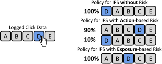
Figure 2. Example comparison of the optimal policy for a single logged click according to three different risk estimators.

Risk in CLTR. Based on the generalization bound proposed in Theorem 4.2, we see that it proposes the following measure of risk: $\text{Risk}(\delta)=\sqrt{\frac{\mathrm{Z}}{N}\big{(}\frac{1-\delta}{\delta}\big{)}d_{2}(\rho\,\|\,\rho_{0})}$ (cf. Eq. 11). Clearly, this risk is mostly determined by the exposure-based divergence between the new policy and the logging policy. Thereby, it states that the greater the difference between how exposure is spread over documents by the logging policy and the new policy, the higher the risk involved. Therefore, to optimize this lower bound, one has to balance the maximization of the estimated utility $\hat{U}(\pi)$ and the minimization of risk by not letting $\pi$ differ too much from $\pi_{0}$ in terms of exposure.

Furthermore, we see that our measure of risk diminishes as $N$ increases. As a result, the risk term will overwhelm the IPS term when $N$ is very low, as there is much risk involved when estimating based on a few interactions. Conversely, when $N$ is very large, the risk term mostly disappears, as the IPS estimate is more reliable when based on large numbers of interactions. Thus, during optimization, the generalization bound is expected to mostly help with avoiding initial decreases in performance, while still converging at the same place as the standard IPS estimator.

Lastly, the $\delta$ parameter determines the safety that is provided by the risk, where a lower $\delta$ makes it more likely that the generalization bound holds. Accordingly, as $\delta$ increases the risk term becomes smaller and will thus have less effect on optimization.

To the best of our knowledge, this is the first exposure-based generalization bound, which makes it the first method designed for safe optimization in the CLTR setting.

Illustrative comparison. To emphasize the working and novelty of our exposure-based risk, a comparison of the optimal policies for action-based risk, exposure-based risk, and no risk are shown in Figure 2. We see that IPS without a risk term places the once-clicked document at the first position, with 100% probability. This is very risky, as it greatly impacts the ranking while only being based on a single observation. The action-based risk tries to mitigate this risk with a probabilistic policy that gives most probability to the logging policy ranking (90%) and the remainder to the IPS ranking (10%). In contrast, with exposure-based risk, the optimal policy makes the risk and utility trade-off in a single ranking, that mostly follows the logging policy but places the clicked document slightly higher.

This example illustrates that because action-based risk does not have a similarity measure between rankings, it can only produce a probabilistic interpolation between the logging policy and IPS rankings. Alternatively, because exposure-based risk does have such a measure, it produces a ranking that is neither the logging ranking nor the IPS ranking, but one with an exposure distribution that is similar to both. Thereby, exposure-based risk has a more elegant and natural method of balancing utility maximization and risk minimization in the CLTR setting.

Table 1. NDCG@5 performance under different settings and datasets for several values of $N$, the number of logged interactions in the simulated training set. Reported numbers are averages over 10 independent runs evaluated on the held-out test-sets, bold numbers indicate the highest performance. Statistical significance for differences with the exposure-based CRM are measured via a two-sided student-t test, ^▼ indicates methods with significantly lower NDCG with $p<0.01$, and ^⋆ no significant difference.

	Yahoo! Webscope			MSLR-WEB30k			Istella
	$N=4\cdot 10^{2}$	$N=4\cdot 10^{7}$	$N=10^{9}$	$N=4\cdot 10^{2}$	$N=4\cdot 10^{7}$	$N=10^{9}$	$N=4\cdot 10^{2}$	$N=4\cdot 10^{7}$	$N=10^{9}$
Logging	0.677 (0.000)-	0.677 (0.000)-	0.677 (0.000)-	0.435 (0.000)-	0.435 (0.000)-	0.435 (0.000)-	0.635 (0.000)-	0.635 (0.000)-	0.635 (0.000)-
Skyline	0.727 (0.000)-	0.727 (0.000)-	0.727 (0.000)-	0.479 (0.000)-	0.479 (0.000)-	0.479 (0.000)-	0.714 (0.000)-	0.714 (0.000)-	0.714 (0.000)-
Naive	0.652 (0.021)▼	0.694 (0.000)▼	0.695 (0.000)▼	0.353 (0.003)▼	0.448 (0.000)▼	0.448 (0.001)▼	0.583 (0.007)▼	0.661 (0.001)▼	0.661 (0.001)▼
Action IPS	0.656 (0.008)▼	0.701 (0.001)▼	0.701 (0.001)▼	0.359 (0.007)▼	0.448 (0.001)▼	0.448 (0.001)▼	0.578 (0.004)▼	0.671 (0.001)▼	0.671 (0.002)▼
Action CRM	0.617 (0.004)▼	0.698 (0.001)▼	0.700 (0.001)▼	0.359 (0.005)▼	0.448 (0.001)▼	0.449 (0.001)▼	0.449 (0.013)▼	0.668 (0.002)▼	0.672 (0.001)▼
Exp. IPS	0.659 (0.010)▼	0.723 (0.001)⋆	0.730 (0.001)⋆	0.389 (0.014)▼	0.474 (0.001)⋆	0.481 (0.001)⋆	0.576 (0.010)▼	0.696 (0.001)⋆	0.706 (0.001)⋆
Exp. CRM	0.677 (0.001)-	0.723 (0.001)-	0.730 (0.000)-	0.434 (0.001)-	0.473 (0.001)-	0.480 (0.001)-	0.635 (0.001)-	0.695 (0.001)-	0.706 (0.001)-

5. A Novel Counterfactual Risk Minimization Method for LTR

Now that we have the proven generalization bound described in Section 4.3 (Theorem 4.2), we can propose a novel risk-aware CLTR method for optimizing it. The aim of our method is to find the policy that maximizes this high-confidence lower bound on the true performance. In formal terms, we have the following optimization problem:

(31) $$\max_{\pi}\hat{U}(\pi)-\sqrt{\frac{\mathrm{Z}}{N}\Big{(}\frac{1-\delta}{\delta}\Big{)}d_{2}(\rho\,\|\,\rho_{0})}.$$

We propose to train a stochastic policy $\pi$ via stochastic gradient descent, therefore, we need to derive the gradient and find a method of computing it. For the computation of the gradient w.r.t. the utility $\hat{U}(\pi)$, the first part of Eq. 31, we refer to several prior work that discusses this topic extensively (Oosterhuis, 2021; Oosterhuis and de Rijke, 2020a; Yadav et al., 2021). Thus, we can focus our attention on the second part of Eq. 31:

(32) $$\nabla_{\!\pi}\sqrt{\frac{\mathrm{Z}}{N}\Big{(}\frac{1-\delta}{\delta}\Big{)}d_{2}(\rho\,\|\,\rho_{0})}=\sqrt{\frac{\mathrm{Z}(1-\delta)}{4N\delta d_{2}(\rho\,\|\,\rho_{0})}}\nabla_{\!\pi}d_{2}(\rho\,\|\,\rho_{0}).$$

To derive the gradient of the exposure-based divergence function, we use the relation between $\rho$ and $\rho^{\prime}$ from Eq. 17 and 18:

(33) $$\begin{split}\nabla_{\!\pi}d_{2}(\rho\,\|\,\rho_{0})&=\nabla_{\!\pi}\mathbb{E}_{q}\bigg{[}\sum_{d\in D_{q}}\!\rho^{\prime}_{0}(d)\left(\frac{\rho^{\prime}(d)}{\rho^{\prime}_{0}(d)}\right)^{2}\bigg{]}\\ &=\frac{2}{\mathrm{Z}}\,\mathbb{E}_{q}\bigg{[}\!\sum_{d\in D_{q}}\!\!\frac{\rho(d)}{\rho_{0}(d)}\nabla_{\!\pi}\rho(d)\bigg{]}.\end{split}$$

Thus, we only need the gradient w.r.t. the exposure of a document ($\nabla_{\!\pi}\rho(d)$) to complete our derivation. If $\pi$ is a Plackett-Luce (PL) ranking model, one can make use of the specialized gradient computation algorithm from (Oosterhuis, 2021). However, for this work, we will not make further assumptions about $\pi$ and apply the more general log-derivate trick from the REINFORCE algorithm (Williams, 1992):

(34) $$\nabla_{\!\pi}\rho(d)=\mathbb{E}_{y\sim\pi}\big{[}P\big{(}E=1\mid\text{rank}(d\mid y)\big{)}\big{]}\nabla_{\!\pi}\log\pi(y).$$

Putting all of the previous elements back together, gives us the gradient w.r.t. the exposure-based risk function:

(35) $$\mbox{}\sqrt{\!\frac{1-\delta}{N\delta\,\mathrm{Z}\,d_{2}(\rho\,\|\,\rho_{0})}}\mathbb{E}_{q,y\sim\pi}\!\left[\!\left(\sum_{k=1}^{K}\!\frac{\rho(y_{k})}{\rho_{0}(y_{k})}P(E=1|\,k)\!\right)\nabla_{\!\pi}\!\log\pi(y)\!\right],\mbox{}$$

where $y_{k}$ is the document at rank $k$ in ranking $y$. For a close approximation of this gradient, we substitute the gradient with the queries from the given dataset, and the rankings sampled from $\pi$ during optimization (Williams, 1992; Oosterhuis, 2021).

Similarly, since the exact computation of is $d_{2}(\rho\,\|\,\rho_{0})$ infeasible in practice, we introduce a sample-based empirical divergence estimator:

(36) $$\hat{d}_{2}(\rho\mid\mid\rho_{0})=\frac{1}{N}\sum_{i=1}^{N}\sum_{d\in D_{q_{i}}}\rho_{0}^{\prime}(d)\left(\frac{\rho^{\prime}(d)}{\rho_{0}^{\prime}(d)}\right)^{2}.$$

This is an unbiased estimate of the true divergence given that the sampling process is truly monte-carlo (James, 1980).

	Yahoo! Webscope	MSLR-WEB30k	Istella
NDCG@5
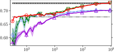
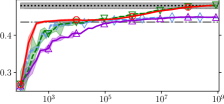
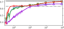
NDCG@5
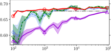
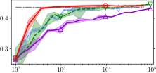
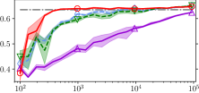
	Number of interactions simulated ($N$)	Number of interactions simulated ($N$)	Number of interactions simulated ($N$)

Figure 3. Performance in NDCG@5 of various IPS and CRM methods for CLTR. The top-row presents the results when the size of the training data is varied from extremely small ($10^{2}$) to extremely high ($10^{9}$). The bottom-row is a zoomed-in view, focusing on the low-data region from $10^{2}$ to $10^{5}$. Results are averages over 10 runs; shaded areas indicate 80% confidence intervals.

6. Experimental Setup

For our experiments, we follow the semi-synthetic experimental setup that is common in the CLTR literature (Oosterhuis and de Rijke, 2021a, b; Joachims et al., 2017; Vardasbi et al., 2020). We make use of the three largest publicly available LTR datasets: Yahoo! Webscope (Chapelle and Chang, 2011), MSLR-WEB30k (Qin and Liu, 2013), and Istella (Dato et al., 2016). The datasets consist of queries, a preselected list of documents per query, query-document feature vectors, and manually-graded relevance judgements for each query-document pair. To generate clicks, we follow previous work (Oosterhuis and de Rijke, 2021a, b; Vardasbi et al., 2020) and train a logging policy on a $3\%$ fraction of the relevance judgements. This simulates a real-world setting, where a production ranker trained on manual judgements is used to collect click logs, which can then be used for subsequent click-based optimization. Typically, in real-world ranking settings, given that the production ranker is used on live-traffic, it is deemed as a safe policy that can be trusted with real users.

We simulate a top-$K$ ranking setup (Oosterhuis and de Rijke, 2020a) where five documents are presented at once. Clicks are generated with our assumed click model (Eq. 3) and the following rank-based position-bias:

(37) $$P(E=1\mid q,d,y)=\begin{cases}\left(\frac{1}{\textrm{rank}(d|y)}\right)^{2}&\text{if }\textrm{rank}(d\mid y)\leq 5,\\ 0&\text{otherwise}.\end{cases}$$

In real-world click data, the observed CTR is typically very low (Saito et al., 2020; Chen et al., 2019; Li et al., 2010); hence, to simulate such a sparse click settings, we apply the following transformation from relevance judgements to relevance probabilities:

(38) $$P(R=1\mid q,d)=0.025*rel(q,d)+0.2,$$

where $rel(q,d)\in\{0,1,2,3,4\}$ is the relevance judgement for the query-document pair and $0.2$ is added as click noise. During training, the only available data consists of clicks generated on the training and validation sets, no baseline method has access to the underlying relevance judgements (expect the skyline).

Furthermore, we assume a setting where the exact logging policy is not available during training. As a result, the $\hat{\rho}_{0}$ propensities have to estimated, we use a simple frequency estimate following (Oosterhuis and de Rijke, 2021a):

(39) $$\hat{\rho}_{0}(d)=\sum^{N}_{i=1}\frac{\mathds{1}\big{[}q=q_{i}\big{]}}{\sum^{N}_{j=1}\mathds{1}\big{[}q=q_{j}\big{]}}P\big{(}E=1\mid\text{rank}(d\mid y_{i})\big{)}.$$

For the action-based baselines, the action propensities $\hat{\pi}_{0}(y\mid q)$ are similarly estimated based on observed frequencies:

(40) $$\hat{\pi}_{0}(y\,|\,q)=\prod_{k=1}^{K-1}\hat{\pi}_{0}(y_{k}\,|\,q),\hskip 2.84526pt\hat{\pi}_{0}(y_{k}\,|\,q)=\sum^{N}_{j=1}\frac{\mathds{1}\big{[}y_{k}=y_{j}]}{\sum^{N}_{j=1}\mathds{1}\big{[}q=q_{j}\big{]}},$$

where $\hat{\pi}_{0}(y_{k}\,|\,q)$ is the estimated probability of $d$ appearing at rank $k$ for query $q$. As is common in CLTR (Oosterhuis, 2020; Saito and Joachims, 2021; Joachims et al., 2017), we clip propensities by $10/\sqrt{N}$ in the training set, to reduce variance, but not in the validation set.

We optimize neural PL ranking models (Oosterhuis, 2021) with early stopping based on validation clicks to prevent overfitting. For the REINFORCE policy-gradient, we follow (Yadav et al., 2021) and use the average reward per query as a control-variate for variance reduction.

As our evaluation metric, we compute NDCG@5 metric using the relevance judgements on the test split of each dataset (Järvelin and Kekäläinen, 2002). All reported results are averages over ten independent runs, significant testing is performed with a two-sided student-t test.

Finally, the following methods are included in our comparisons:

1. Naive. As the most basic baseline, we train on the generated clicks without any correction (equivalent to $\forall d,\,\rho_{0}(d)=1$).

2. Skyline. To compare with the highest possible performance, this baseline is trained on the actual relevance judgements.

3. Action-based IPS. Standard IPS estimation (Eq. 13) that is not designed for ranking and thus uses action-based propensities.

4. Action-based CRM. Standard CRM (Eq. 12) that is also not designed for ranking, for the risk function we use the action-based divergence function in Eq. 15.

5. Exposure-based IPS. The IPS estimator designed for CLTR with exposure-based propensities (Eq. 7). The most important baseline, as it is the prevalent approach in the field (Oosterhuis and de Rijke, 2020a, 2021a).

6. Exposure-based CRM. Our proposed CRM method (Eq. 31) using a risk function based on exposure-based divergence.

7. Results and Discussion

7.1. Comparison with baseline methods

The main results of our experimental comparison are presented in Figure 3 and Table 3. Figure 3 displays the performance curves of the different methods as the number of logged interactions ($N$) increases. Table 3 presents performance at $N\in\{4\cdot 10^{2},4\cdot 10^{7},10^{9}\}$ and indicates whether the observed differences with our exposure-based CRM method are statistically significant.

We start by considering the performance curves in Figure 3. We see that both the action-based and exposure-based IPS baselines have an initial period of very similar performance that is far below the logging policy. Around $N\approx 10^{4}$ their performance is comparable to the logging policy, and finally at $N=10^{9}$ the exposure-based IPS has reached optimal performance, while the performance of action-based IPS is still far from optimal. We can attribute this initial poor performance to the high variance problem of IPS estimation; when $N$ is small, variance is at its highest, resulting in risky and sub-optimal optimization by the IPS estimators. However, even when $N=10^{9}$, the variance of the action-based IPS estimator is too high to reach optimal performance, due to its extremely small propensities. This illustrates why the introduction of exposure-based propensities was so important to the CLTR field, and that even exposure-based IPS produces unsafe optimization when little data is available or variance from interactions is high.

Next, we consider whether action-based CRM is able to mitigate the high variance problem of action-based IPS. Despite being a proven generalization bound, Figure 3 clearly shows us that action-based CRM only leads to decreases in performance compared to its IPS counterpart. It appears that this happens because the logging policy is not available in our setup, and the propensities have to be estimated from logged data. Consequently, the action-based risk pushes the optimization to mimic the exact rankings that were observed during logging. Thus, due to the variance introduced from the sampling of rankings from the logging policy, it appears that action-based CRM has an even higher variance problem than action-based IPS. As expected, our results thus clearly indicate that action-based CRM is also unsuited for the CLTR setting, to our surprise; it is substantially worse than its IPS counterpart.

Finally, we examine the performance of our novel exposure-based CRM method. Similar to the other methods, there is an initial period of low performance, but in stark contrast, this period ends very quickly; on Yahoo! logging policy performance is reached when $N\approx 125$, on MSLR-WEB30k when $N\approx 350$ and on Istella when $N\approx 400$. For comparison, exposure-based IPS needs $N\approx 1100$ on Yahoo!, $N\approx 10^{4}$ on MLSR-WEB30k and $N\approx 1.1\cdot 10^{4}$ on Istella to do the same; meaning that our CRM method needs roughly $89\%$, $97\%$ and $97\%$ fewer interactions, respectively. In addition, Table 3 indicates that the logging policy performance is matched on all datasets when $N=400$ by exposure-based CRM, where it also outperforms all baseline methods. We note that there is still an initial period of low performance, because the logging policy is unavailable at training, and thus, its behavior still has to be estimated from logged interactions. It is possible that in settings where the logging policy is fully known during training, this initial period is eliminated entirely. Nevertheless, our results show that exposure-based CRM reduces the initial periods of poor performance due to variance by an enormous magnitude.

	Yahoo! Webscope	MSLR-WEB30k	Istella
Action-based CRM NDCG@5
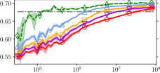
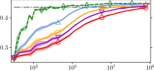
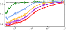
Exposure-based CRM NDCG@5
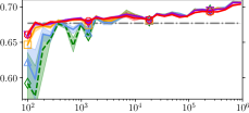
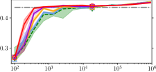
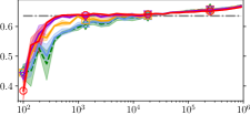
	Number of interactions simulated ($N$)	Number of interactions simulated ($N$)	Number of interactions simulated ($N$)

Figure 4. Performance of CRM methods with varying confidence parameters ($\delta$). Top-row: action-based CRM baseline; bottom-row: our exposure-based CRM method. Results are averages of 10 runs; shaded areas indicate 80% confidence intervals.

Furthermore, while the initial period is clearly improved, we should also consider whether there is a trade-off with the rate of convergence. Surprisingly, Figure 3 does not display any noticeable decrease in performance when compared with exposure-based IPS. Moreover, Table 3 shows the differences between exposure-based IPS and CRM are barely measurable and not statistically significant when $N\in\{4\cdot 10^{7},10^{9}\}$. We know from the risk formulation in Eq. 31 that the weight of the risk term decreases as $N$ increases at a rate of $1/\sqrt{N}$. In other words, the more data is available, the more optimization is able to diverge from the logging policy. It appears that this balances utility maximization and risk minimization so well that we are unable to observe any downside of applying exposure-based CRM instead of IPS. Therefore, we conclude that, compared to all baseline methods and across all datasets, exposure-based CRM drastically reduces the initial period of low performance, matches the best rate of convergence of all baseline, and has optimal performance at convergence.

7.2. Ablation study on the confidence parameter

To gain insights into how the confidence parameter $\delta$ affects the trade-off between safety and utility, an ablation study over various $\delta$ values was performed for both CRM methods.

The top-row of Figure 4 shows us the performance of action-based CRM, and contrary to expectation, a decrease in $\delta$ corresponds to a considerably worse performance. For the sake of clarity, in theory, $\delta$ is inversely tied to safety, a lower $\delta$ should result in less divergence from the safe logging policy (Oosterhuis and de Rijke, 2021b). Conversely, we see that action-based CRM displays the opposite trend. We think this further confirms our hypothesis that a frequency estimate of action-based divergence has an even higher variance problem than action-based IPS. Consequently, a higher weight to the risk function results in worse performance. This further confirms our previous conclusion that action-based CRM is unsuited for the CLTR setting, regardless of how the $\delta$ parameter is tuned.

In contrast, the bottom-row of Figure 4 displays the expected trend for exposure-based CRM; as $\delta$ decreases the resulting performance gets closer to the logging policy. With $\delta=0.1$, CRM performs extremely close to its IPS counterpart, as optimization is less constrained to mimic the logging policy here. Decreasing $\delta$ appears to have diminishing returns, as the difference between $\delta=10^{-4}$ and $\delta=10^{-5}$ is marginal. Importantly, we do not observe any downsides to setting $\delta=10^{-5}$, thus we have not reached a point in our experiments where $\delta$ is set too conservatively. This suggests that exposure-based CRM is very robust to the setting of the $\delta$ parameter, and that a sufficiently low $\delta$ does not require fine-tuning. Therefore, this shows that the improvements we observed when comparing with baseline methods, did not stem from a fine-tuning of $\delta$. Thus, we can conclude that this robustness further increases the safety that is provided by exposure-based CRM, as there is also little risk involved in the tuning of the $\delta$ parameter.

8. Conclusion

In this paper, we introduced the first counterfactual risk minimization (CRM) method designed for CLTR, that relies on a novel exposure-based divergence function. In contrast with existing action-based CRM methods, exposure-based divergence avoids the problem of the enormous combinatorial action space when ranking, by measuring the dissimilarity between policies based on how they distribute exposure to documents. As a result, exposure-based CRM optimization produces policies that rank similar to the logging policy when it is risky to follow IPS, i.e., when little data is available or variance is very high. Consequently, our experimental results show that it almost completely removes initial periods of detrimental performance; to be precise, our method needed 89% to 97% fewer interactions than state-of-the-art IPS to match production system performance. Importantly, we observed no downsides in its application, as it maintained the same rate and point of convergence as IPS, in all tested experimental settings. Therefore, we conclude that our exposure-based CRM method provides the safest CLTR methods so far, as it almost completely alleviates the risk of decreasing the performance of a production system.

These improvements have large implications for practitioners who work on ranking systems in real-world settings, since the almost complete reduction of initial detrimental performance removes the main risks involved in applying CLTR. In other words, when applying our novel exposure-based CRM, practitioners can have significantly less worry that the resulting policy will perform worse than their production system and hurt user experience.

We hope future work will further research the promising potential applications of exposure-based CRM, for instance, in settings with fast turn-around times in deployment, or large numbers of tail-queries (Wedig and Madani, 2006; White et al., 2007), where interaction data is limited.

Reproducibility

All experimental results in this work were obtained using publicly available data. Our implementation is publicly available at https://github.com/shashankg7/crm_ultr.

References

- (1)
- Agarwal et al. (2019) Aman Agarwal, Xuanhui Wang, Cheng Li, Michael Bendersky, and Marc Najork. 2019. Addressing Trust Bias for Unbiased Learning-to-rank. In The World Wide Web Conference. 4–14.
- Chapelle and Chang (2011) Olivier Chapelle and Yi Chang. 2011. Yahoo! Learning to Rank Challenge Overview. In Proceedings of the learning to rank challenge. PMLR, 1–24.
- Chapelle and Zhang (2009) Olivier Chapelle and Ya Zhang. 2009. A Dynamic Bayesian Network Click Model for Web Search Ranking. In Proceedings of the 18th international conference on World wide web. 1–10.
- Chen et al. (2019) Jia Chen, Jiaxin Mao, Yiqun Liu, Min Zhang, and Shaoping Ma. 2019. TianGong-ST: A New Dataset with Large-scale Refined Real-world Web Search Sessions. In Proceedings of the 28th ACM International Conference on Information and Knowledge Management. 2485–2488.
- Chuklin et al. (2015) Aleksandr Chuklin, Ilya Markov, and Maarten de Rijke. 2015. Click Models for Web Search. Morgan & Claypool Publishers.
- Cortes et al. (2010) Corinna Cortes, Yishay Mansour, and Mehryar Mohri. 2010. Learning Bounds for Importance Weighting. In Proceedings of the 23rd International Conference on Neural Information Processing Systems-Volume 1. 442–450.
- Craswell et al. (2008) Nick Craswell, Onno Zoeter, Michael Taylor, and Bill Ramsey. 2008. An Experimental Comparison of Click Position-bias Models. In Proceedings of the 2008 international conference on web search and data mining. 87–94.
- Dato et al. (2016) Domenico Dato, Claudio Lucchese, Franco Maria Nardini, Salvatore Orlando, Raffaele Perego, Nicola Tonellotto, and Rossano Venturini. 2016. Fast Ranking with Additive Ensembles of Oblivious and Non-Oblivious Regression Trees. ACM Transactions on Information Systems (TOIS) 35, 2 (2016), 1–31.
- Ghosh (2002) BK Ghosh. 2002. Probability Inequalities Related to Markov’s Theorem. The American Statistician 56, 3 (2002), 186–190.
- He et al. (2019) Li He, Long Xia, Wei Zeng, Zhi-Ming Ma, Yihong Zhao, and Dawei Yin. 2019. Off-policy Learning for Multiple Loggers. In Proceedings of the 25th ACM SIGKDD International Conference on Knowledge Discovery & Data Mining. 1184–1193.
- Horvitz and Thompson (1952) Daniel G Horvitz and Donovan J Thompson. 1952. A Generalization of Sampling Without Replacement From a Finite Universe. Journal of the American statistical Association 47, 260 (1952), 663–685.
- Jagerman et al. (2020) Rolf Jagerman, Ilya Markov, and Maarten de Rijke. 2020. Safe Exploration for Optimizing Contextual Bandits. ACM Transactions on Information Systems (TOIS) 38, 3 (2020), 1–23.
- James (1980) Frederick James. 1980. Monte Carlo Theory and Practice. Reports on progress in Physics 43, 9 (1980), 1145.
- Järvelin and Kekäläinen (2002) Kalervo Järvelin and Jaana Kekäläinen. 2002. Cumulated Gain-Based Evaluation of IR Techniques. ACM Transactions on Information Systems (TOIS) 20, 4 (2002), 422–446.
- Jiang et al. (2016) Shan Jiang, Yuening Hu, Changsung Kang, Tim Daly Jr, Dawei Yin, Yi Chang, and Chengxiang Zhai. 2016. Learning Query and Document Relevance from a Web-scale Click Graph. In Proceedings of the 39th International ACM SIGIR conference on Research and Development in Information Retrieval. 185–194.
- Joachims (2002) Thorsten Joachims. 2002. Optimizing Search Engines Using Clickthrough Data. In Proceedings of the eighth ACM SIGKDD international conference on Knowledge discovery and data mining. 133–142.
- Joachims and Swaminathan (2016) Thorsten Joachims and Adith Swaminathan. 2016. Counterfactual Evaluation and Learning for Search, Recommendation and Ad Placement. In Proceedings of the 39th International ACM SIGIR conference on Research and Development in Information Retrieval. 1199–1201.
- Joachims et al. (2017) Thorsten Joachims, Adith Swaminathan, and Tobias Schnabel. 2017. Unbiased Learning-to-rank with Biased Feedback. In Proceedings of the Tenth ACM International Conference on Web Search and Data Mining. 781–789.
- Li et al. (2010) Lihong Li, Wei Chu, John Langford, and Robert E Schapire. 2010. A Contextual-Bandit Approach to Personalized News Article Recommendation. In Proceedings of the 19th international conference on World wide web. 661–670.
- Liu (2009) Tie-Yan Liu. 2009. Learning to Rank for Information Retrieval. Foundations and Trends® in Information Retrieval 3, 3 (2009), 225–331.
- Maurer and Pontil (2009) Andreas Maurer and Massimiliano Pontil. 2009. Empirical Bernstein Bounds and Sample-Variance Penalization. In Annual Conference Computational Learning Theory.
- Nowozin et al. (2016) Sebastian Nowozin, Botond Cseke, and Ryota Tomioka. 2016. f-GAN: Training Generative Neural Samplers using Variational Divergence Minimization. Advances in neural information processing systems 29 (2016).
- Oosterhuis (2020) Harrie Oosterhuis. 2020. Learning from User Interactions with Rankings: A Unification of the Field. Ph. D. Dissertation. Informatics Institute, University of Amsterdam.
- Oosterhuis (2021) Harrie Oosterhuis. 2021. Computationally Efficient Optimization of Plackett-Luce Ranking Models for Relevance and Fairness. In Proceedings of the 44th International ACM SIGIR Conference on Research and Development in Information Retrieval. 1023–1032.
- Oosterhuis (2022a) Harrie Oosterhuis. 2022a. Doubly-Robust Estimation for Unbiased Learning-to-Rank from Position-Biased Click Feedback. arXiv preprint arXiv:2203.17118 (2022).
- Oosterhuis (2022b) Harrie Oosterhuis. 2022b. Reaching the End of Unbiasedness: Uncovering Implicit Limitations of Click-Based Learning to Rank. In Proceedings of the 2022 ACM SIGIR International Conference on the Theory of Information Retrieval. ACM.
- Oosterhuis and de Rijke (2020a) Harrie Oosterhuis and Maarten de Rijke. 2020a. Policy-aware Unbiased Learning to Rank for Top-k Rankings. In Proceedings of the 43rd International ACM SIGIR Conference on Research and Development in Information Retrieval. 489–498.
- Oosterhuis and de Rijke (2020b) Harrie Oosterhuis and Maarten de Rijke. 2020b. Taking the Counterfactual Online: Efficient and Unbiased Online Evaluation for Ranking. In Proceedings of the 2020 ACM SIGIR on International Conference on Theory of Information Retrieval. 137–144.
- Oosterhuis and de Rijke (2021a) Harrie Oosterhuis and Maarten de Rijke. 2021a. Unifying Online and Counterfactual Learning to Rank: A Novel Counterfactual Estimator that Effectively Utilizes Online Interventions. In Proceedings of the 14th ACM International Conference on Web Search and Data Mining. 463–471.
- Oosterhuis and de Rijke (2021b) Harrie Oosterhuis and Maarten de de Rijke. 2021b. Robust Generalization and Safe Query-Specialization in Counterfactual Learning to Rank. In Proceedings of the Web Conference 2021. 158–170.
- Oosterhuis et al. (2020) Harrie Oosterhuis, Rolf Jagerman, and Maarten de Rijke. 2020. Unbiased Learning to Rank: Counterfactual and Online Approaches. In Companion Proceedings of the Web Conference 2020. 299–300.
- Qin and Liu (2013) Tao Qin and Tie-Yan Liu. 2013. Introducing LETOR 4.0 Datasets. arXiv preprint arXiv:1306.2597 (2013).
- Qin et al. (2010) Tao Qin, Tie-Yan Liu, Jun Xu, and Hang Li. 2010. LETOR: A Benchmark Collection for Research on Learning to Rank for Information Retrieval. Information Retrieval 13, 4 (2010), 346–374.
- Radlinski et al. (2008) Filip Radlinski, Madhu Kurup, and Thorsten Joachims. 2008. How Does Clickthrough Data Reflect Retrieval Quality?. In Proceedings of the 17th ACM conference on Information and knowledge management. 43–52.
- Rényi (1961) Alfréd Rényi. 1961. On measures of entropy and information. In Proceedings of the fourth Berkeley symposium on mathematical statistics and probability, Vol. 1. Berkeley, California, USA.
- Saito et al. (2020) Yuta Saito, Shunsuke Aihara, Megumi Matsutani, and Yusuke Narita. 2020. Open Bandit Dataset and Pipeline: Towards Realistic and Reproducible Off-Policy Evaluation. arXiv preprint arXiv:2008.07146 (2020).
- Saito and Joachims (2021) Yuta Saito and Thorsten Joachims. 2021. Counterfactual Learning and Evaluation for Recommender Systems: Foundations, Implementations, and Recent Advances. In Fifteenth ACM Conference on Recommender Systems. 828–830.
- Sanderson et al. (2010) Mark Sanderson, Monica Lestari Paramita, Paul Clough, and Evangelos Kanoulas. 2010. Do User Preferences and Evaluation Measures Line Up?. In Proceedings of the 33rd international ACM SIGIR conference on Research and development in information retrieval. 555–562.
- Shalev-Shwartz and Ben-David (2014) Shai Shalev-Shwartz and Shai Ben-David. 2014. Understanding Machine Learning: From Theory to Algorithms. Cambridge university press.
- Speretta and Gauch (2005) Mirco Speretta and Susan Gauch. 2005. Personalized Search Based on User Search Histories. In The 2005 IEEE/WIC/ACM International Conference on Web Intelligence (WI’05). IEEE, 622–628.
- Swaminathan and Joachims (2015) Adith Swaminathan and Thorsten Joachims. 2015. Batch Learning from Logged Bandit Feedback through Counterfactual Risk Minimization. The Journal of Machine Learning Research 16, 1 (2015), 1731–1755.
- Thomas et al. (2015) Philip Thomas, Georgios Theocharous, and Mohammad Ghavamzadeh. 2015. High-Confidence Off-Policy Evaluation. In Proceedings of the AAAI Conference on Artificial Intelligence, Vol. 29.
- Vardasbi et al. (2020) Ali Vardasbi, Harrie Oosterhuis, and Maarten de Rijke. 2020. When Inverse Propensity Scoring does not Work: Affine Corrections for Unbiased Learning to Rank. In Proceedings of the 29th ACM International Conference on Information & Knowledge Management. 1475–1484.
- Wang et al. (2016) Xuanhui Wang, Michael Bendersky, Donald Metzler, and Marc Najork. 2016. Learning to Rank with Selection Bias in Personal Search. In Proceedings of the 39th International ACM SIGIR conference on Research and Development in Information Retrieval. ACM, 115–124.
- Wang et al. (2018) Xuanhui Wang, Nadav Golbandi, Michael Bendersky, Donald Metzler, and Marc Najork. 2018. Position Bias Estimation for Unbiased Learning to Rank in Personal Search. In Proceedings of the Eleventh ACM International Conference on Web Search and Data Mining. 610–618.
- Wedig and Madani (2006) Steve Wedig and Omid Madani. 2006. A Large-Scale Analysis of Query Logs for Assessing Personalization Opportunities. In Proceedings of the 12th ACM SIGKDD international conference on Knowledge discovery and data mining. 742–747.
- White et al. (2007) Ryen W White, Mikhail Bilenko, and Silviu Cucerzan. 2007. Studying the Use of Popular Destinations to Enhance Web Search Interaction. In Proceedings of the 30th annual international ACM SIGIR conference on Research and development in information retrieval. 159–166.
- Williams (1992) Ronald J Williams. 1992. Simple Statistical Gradient-Following Algorithms for Connectionist Reinforcement Learning. Machine learning 8, 3 (1992), 229–256.
- Wu and Wang (2018) Hang Wu and May Wang. 2018. Variance Regularized Counterfactual Risk Minimization via Variational Divergence Minimization. In International Conference on Machine Learning. PMLR, 5353–5362.
- Yadav et al. (2021) Himank Yadav, Zhengxiao Du, and Thorsten Joachims. 2021. Policy-Gradient Training of Fair and Unbiased Ranking Functions. In Proceedings of the 44th International ACM SIGIR Conference on Research and Development in Information Retrieval. 1044–1053.