Conditional Graph Information Bottleneck for Molecular Relational Learning

Abstract

Molecular relational learning, whose goal is to learn the interaction behavior between molecular pairs, got a surge of interest in molecular sciences due to its wide range of applications. Recently, graph neural networks have recently shown great success in molecular relational learning by modeling a molecule as a graph structure, and considering atom-level interactions between two molecules. Despite their success, existing molecular relational learning methods tend to overlook the nature of chemistry, i.e., a chemical compound is composed of multiple substructures such as functional groups that cause distinctive chemical reactions. In this work, we propose a novel relational learning framework, called CGIB, that predicts the interaction behavior between a pair of graphs by detecting core subgraphs therein. The main idea is, given a pair of graphs, to find a subgraph from a graph that contains the minimal sufficient information regarding the task at hand conditioned on the paired graph based on the principle of conditional graph information bottleneck. We argue that our proposed method mimics the nature of chemical reactions, i.e., the core substructure of a molecule varies depending on which other molecule it interacts with. Extensive experiments on various tasks with real-world datasets demonstrate the superiority of CGIB over state-of-the-art baselines. Our code is available at https://github.com/Namkyeong/CGIB.

1 Introduction

Figure 1: (a) Molecules with hydroxyl group tend to have high aqueous solubility. (b) C-CF3 structure decreases the solubility of molecules in water. (c) However, it may not be crucial in determining the solubility of molecules in oil.

Relational learning (Rozemberczki et al., 2021), which aims to predict the interaction behavior between entity pairs, got a surge of interest among researchers due to its wide range of applications, especially in molecular science, which is the main focus of this paper. For example, predicting optical and photophysical properties of chromophores with various solvents (i.e., chromophore-solvent pair) is important in designing and synthesizing new colorful materials (Joung et al., 2021). Moreover, it is crucial to determine how medications will dissolve in various solvents (i.e., medication-solvent pair) and how different drug combinations will interact with each other (i.e., drug-drug pair) (Pathak et al., 2020; Wang et al., 2021). Due to the expensive time/financial costs of exhaustively conducting experiments to test the interaction behavior between all possible molecular pairs (Preuer et al., 2018), machine learning approaches have been rapidly adopted for relational learning in molecular sciences (Joung et al., 2021; Pathak et al., 2020; Wang et al., 2021).

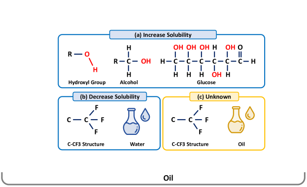
In this paper, we propose a novel molecular relational learning framework inspired by the nature of chemistry: a chemical compound is composed of multiple substructures such as functional groups that cause distinctive chemical reactions. That is, a certain functional group is known to induce the same or similar chemical reactions regardless of other components that exist in the chemical, and thus considering functional groups facilitates a systematic prediction of chemical reactions and the behavior of chemical compounds (Book, 2014; Jerry, 1992). For example, as shown in Figure 1(a), alcohol and glucose commonly contain hydroxyl group, which increases the polarity of molecules. Thus, alcohol and glucose tend to have high aqueous solubility due to the hydroxyl group (Delaney, 2004). In this regard, it is crucial for a model to detect the core substructures of chemicals to improve its generalization ability. However, detecting the core subgraph (i.e., substructure) of an input graph (i.e., chemical compound) is not trivial due to its complex nature (Alsentzer et al., 2020; Meng et al., 2018).

Recently, information bottleneck (IB) theory (Tishby et al., 2000) has been applied to learning significant subgraphs of the input graph for explainable GNNs (Yu et al., 2022, 2020; Miao et al., 2022), which provides a principled approach to determine which aspects of data should be preserved and which should be discarded (Pan et al., 2021). Specifically, GSAT (Miao et al., 2022) formulates the subgraph attention as an information bottleneck by learning stochastic attention that randomly drops edges and obtains a perturbed graph which is considered as an explanatory subgraph. Moreover, VGIB (Yu et al., 2022) obtains a perturbed graph by selectively injecting noises into unnecessary node representations, thereby modulating the information flow from the original graph into the perturbed graph.

However, directly applying graph information bottleneck (GIB) into a relational learning framework is challenging since the complexity arises not only within a single graph, but also between graphs. Specifically, there exist several meaningful subgraphs within a graph, and the importance of each subgraph varies depending on which other graph it interacts with. For example, while C-CF3 substructure plays an important role in decreasing the solubility of molecules in water (Purser et al., 2008) (Figure 1(b)), it may not be crucial in determining the solubility of molecules in oil (Figure 1(c)). This implies that the importance of a substructure depends on the context.

To this end, we propose Conditional Graph Information Bottleneck (CGIB), a simple yet effective relational learning framework that predicts the interaction behavior between a pair of graphs by detecting important subgraphs therein. Our main goal is, given a pair of graphs $\mathcal{G}^{1}$ and $\mathcal{G}^{2}$, to detect the subgraph of $\mathcal{G}^{1}$ (i.e., $\mathcal{G}_{\mathrm{CIB}}^{1}$) that is crucial in determining the interaction behavior between $\mathcal{G}^{1}$ and $\mathcal{G}^{2}$. Existing GIB-based approaches are designed for tasks that require a single input graph, and thus the core subgraph is learned solely based on the input graph itself (Yu et al., 2020, 2022; Miao et al., 2022). On the other hand, as CGIB is designed for relational learning, the core subgraph learned by CGIB varies according to the pair of graphs at hand (i.e., the core subgraph of $\mathcal{G}^{1}$ varies depending on the paired graph $\mathcal{G}^{2}$). Specifically, given a graph $\mathcal{G}^{1}$, CGIB learns its core subgraph $\mathcal{G}^{1}_{\mathrm{CIB}}$ that maximizes the mutual information between a pair of graphs (i.e., ($\mathcal{G}_{\mathrm{CIB}}^{1}$, $\mathcal{G}^{2}$)) and the target response (i.e., $\mathbf{Y}$) we aim to predict, while minimizing the mutual information between the graph $\mathcal{G}^{1}$ and its subgraph $\mathcal{G}^{1}_{\mathrm{CIB}}$ conditioned on its paired graph $\mathcal{G}^{2}$. Moreover, based on the chain rule of mutual information, the conditional mutual information is minimized by injecting Gaussian noise into the node representations of $\mathcal{G}^{1}$, which controls the information flow between the graph and its subgraph $\mathcal{G}^{1}_{\mathrm{CIB}}$, while maximizing the mutual information between the subgraph $\mathcal{G}^{1}_{\mathrm{CIB}}$ and the paired graph $\mathcal{G}^{2}$. By doing so, CGIB learns the subgraph $\mathcal{G}^{1}_{\mathrm{CIB}}$ that contains minimal sufficient information regarding both the paired graph $\mathcal{G}^{2}$ and the target value $\mathbf{Y}$.

Our extensive experiments on eleven real-world datasets on various tasks, i.e., molecular interaction prediction, drug-drug interaction prediction, and graph similarity learning, demonstrate the effectiveness and generality of CGIB in relational learning problems. Moreover, ablation studies verify that CGIB successfully adopts the IB principle to relational learning, which is non-trivial. A further appeal of CGIB is its explainability, i.e., discovering the core substructure of the chemical compounds during chemical reactions, as shown in our qualitative analysis. To the best of our knowledge, CGIB is the first work that adopts the IB principle to relational learning tasks.

2 Related Work

2.1 Molecular Relational Learning

Molecular relational learning can be categorized into two categories according to the target types, i.e., molecular interaction prediction and drug-drug interaction prediction.

Molecular Interaction Prediction. In the molecular interaction prediction task, a model predicts the properties of chemicals induced by chemical reactions or properties of the reaction itself. Delfos (Lim & Jung, 2019) predicts the solvation free energy, which is directly related to the solubility of chemical entities, by using recurrent neural networks and attention mechanisms with SMILES sequence as the input. CIGIN (Pathak et al., 2020) leverages message passing neural networks (Gilmer et al., 2017) and co-attention mechanism to encode the representation of atoms to predict the solvation free energy. Moreover, CIGIN further enhances the interpretability of chemical reactions with co-attention map, which indicates the importance of interaction between atoms. Joung et al. (2021) predict diverse optical and photophysical properties of chromophores, which play a critical role in synthesizing new colorful materials, with the representations of chromophores and solvents that are from graph convolutional networks (Kipf & Welling, 2016).

Drug-Drug Interaction. In the drug-drug interaction task, the model classifies which type of interaction will occur between drugs. Specifically, under the assumption that drugs sharing similar structures tend to share similar interactions, Vilar et al. (2012) and Kastrin et al. (2018) predict DDI by comparing the Tanimoto coefficient of drug fingerprints and exhibiting explicit similarity-based features, respectively. MHCADDI (Deac et al., 2019) proposes a co-attentitive message passing network (Veličković et al., 2017) for polypharmacy side effect prediction, which, given a pair of molecules, aggregates the messages not only from the atoms inside a single molecule, but also all atoms in the paired molecule. MIRACLE (Wang et al., 2021) casts the DDI task as a link prediction task by constructing a multi-view graph, where each node in the interaction graph itself is a drug molecular graph instance.

However, existing studies in molecular relational learning do not consider core substructures such as functional groups, which determine distinctive chemical characteristics. Moreover, they are designed for a specific task, raising doubts on the generality of methods. In this work, we propose a general framework that predicts the behavior of graph pairs by detecting core subgraphs therein.

2.2 Graph Information Bottleneck

Recent studies have introduced the IB principle to graph-structure data, whose irregular data structure incurs unique challenges in computing the mutual information (Yu et al., 2020, 2022; Miao et al., 2022; Sun et al., 2022; Wu et al., 2020). Specifically, GIB (Wu et al., 2020) extends the general IB principle for node representation learning by regularizing both structure and feature information. GIB (Yu et al., 2020) studies the subgraph recognition problem by formulating a subgraph as a bottleneck random variable. It employs the Shannon mutual information to measure how compressed and informative the subgraph distribution is. VGIB (Yu et al., 2022) further stabilizes the subgraph recognition process by injecting Gaussian noise into node representations, where the noise modulates the information flow from the original graph into the perturbed graph. GSAT (Miao et al., 2022) obtains a subgraph by applying stochastic attention, which randomly drops edges with parameterized Bernoulli distribution. Although the IB principle has been successfully applied to graph-structured data, previous studies have focused on tasks that require a single input graph, and thus have only taken into account a single graph for subgraph recognition, which limits their applicability to relational learning tasks. To the best of our knowledge, CGIB is the first work that adopts the IB principle for relational learning.

3 Preliminaries

In this section, we first formally describe the problem formulation including notations and the task description (Section 3.1). Then, we introduce definitions of IB and IB-Graph, which is an application of IB to recognize the core subgraph of an input graph (Section 3.2).

3.1 Problem Formulation

Notations. Let $\mathcal{G}=(\mathcal{V},\mathcal{E})$ denotes a graph, where $\mathcal{V}=\{v_{1},\ldots,v_{N}\}$ represents the set of nodes, and $\mathcal{E}\subseteq\mathcal{V}\times\mathcal{V}$ represents the set of edges. $\mathcal{G}$ is associated with a feature matrix $\mathbf{X}\in\mathbb{R}^{N\times F}$, and an adjacency matrix $\mathbf{A}\in\mathbb{R}^{N\times N}$ where $\mathbf{A}_{ij}=1$ if and only if $(v_{i},v_{j})\in\mathcal{E}$ and $\mathbf{A}_{ij}=0$ otherwise. We denote $I(X;Y)$ as the mutual information between random variables $X$ and $Y$:

$$I(X;Y)=\int_{X}\int_{Y}p(x,y)\log\frac{p(x,y)}{p(x)p(y)}dxdy$$ (1)

Task: Relational Learning on Graphs. Given a set of graph pairs $\mathcal{D}=\{(\mathcal{G}_{1}^{1},\mathcal{G}_{1}^{2}),(\mathcal{G}_{2}^{1},\mathcal{G}_{2}^{2}),\ldots,(\mathcal{G}_{n}^{1},\mathcal{G}_{n}^{2})\}$ and the associated target values $\mathbb{Y}=\{\mathbf{Y}_{1},\mathbf{Y}_{2},\ldots,\mathbf{Y}_{n}\}$, our goal is to train a model $\mathcal{M}$ that predicts the target values of given arbitrary graph pairs in an end-to-end manner, i.e., $\mathbf{Y}_{i}=\mathcal{M}(\mathcal{G}_{i}^{1},\mathcal{G}_{i}^{2})$. The target $\mathbf{Y}$ is a scalar value, i.e., $\mathbf{Y}\in(-\infty,\infty)$, for regression tasks, while it is a binary class label, i.e., $\mathbf{Y}\in\{0,1\}$, for (binary) classification tasks.

3.2 Information Bottleneck

In machine learning, it is important to determine which aspects of the input data should be preserved and which should be discarded. Information bottleneck (IB) (Tishby et al., 2000) provides a principled approach to this problem, compressing the source random variable to keep the information relevant for predicting the target random variable while discarding target-irrelevant information.

Definition 3.1.

(Information Bottleneck) Given random variables $X$ and $Y$, the Information Bottleneck principle aims to compress $X$ to a bottleneck random variable $T$, while keeping the information relevant for predicting $Y$:

$$\min_{T}-I(Y;T)+\beta I(X;T)$$ (2)

where $\beta$ is a Lagrangian multiplier for balancing the two mutual information terms.

Recently, IB principle has been applied to learning a bottleneck graph $\mathcal{G}_{\mathrm{IB}}=(\mathbf{X}_{\mathrm{IB}},\mathbf{A}_{\mathrm{IB}})$ named IB-Graph for $\mathcal{G}$, which keeps minimal sufficient information in terms of $\mathcal{G}$’s properties (Yu et al., 2020, 2022; Miao et al., 2022).

Definition 3.2.

(IB-Graph) For a graph $\mathcal{G}=(\mathbf{X},\mathbf{A})$ and its label information $\mathbf{Y}$, the optimal graph $\mathcal{G}_{\mathrm{IB}}=(\mathbf{X}_{\mathrm{IB}},\mathbf{A}_{\mathrm{IB}})$ discovered under the IB principle is denoted as IB-Graph:

$$\mathcal{G}_{\mathrm{IB}}=\operatorname*{arg\,min}_{\mathcal{G}_{\mathrm{IB}}}-I(\mathbf{Y};\mathcal{G}_{\mathrm{IB}})+\beta I(\mathcal{G};\mathcal{G}_{\mathrm{IB}})$$ (3)

where $\mathbf{X}_{\mathrm{IB}}$ and $\mathbf{A}_{\mathrm{IB}}$ denote the task-relevant feature set and the adjacency matrix of $\mathcal{G}$, respectively.

Intuitively, graph information bottleneck (GIB) aims to learn the core subgraph of the input graph (i.e., $\mathcal{G}_{\mathrm{IB}}$), which discards information from the input graph by minimizing the term $I(\mathcal{G};\mathcal{G}_{\mathrm{IB}})$, while preserving target-relevant information by maximizing the term $I(\mathbf{Y};\mathcal{G}_{\mathrm{IB}})$.

4 Methodology

In this section, we introduce our proposed method called CGIB, a novel relational learning framework that detects the core subgraph of an input graph based on the conditional mutual information. First, we formally define the conditional graph information bottleneck and CIB-Graph (Section 4.1). Then, we introduce the overall model architecture (Section 4.2) followed by the overall optimization process of CGIB (Section 4.3).

Figure 2: Overall model architecture.

4.1 Conditional Graph Information Bottleneck

In this work, we are interested in learning the core subgraph $\mathcal{G}_{\mathrm{CIB}}^{1}=(\mathbf{X}_{\mathrm{CIB}}^{1},\mathbf{A}_{\mathrm{CIB}}^{1})$ of input graph $\mathcal{G}^{1}$ conditioned on the paired input graph $\mathcal{G}^{2}$.

Definition 4.1.

(Conditional Information Bottleneck) Given random variables $X^{1},X^{2}$, and $Y$, the Conditional Information Bottleneck (CIB) principle aims to compress $X^{1}$ to a bottleneck random variable $T^{1}$, while keeping the information relevant for predicting $Y$ conditioned on the random variable $X^{2}$:

$$\small\min_{T^{1}}-I(Y;T^{1}|X^{2})+\beta I(X^{1};T^{1}|X^{2})$$ (4)

where $\beta$ is a Lagrangian multiplier for balancing the two conditional mutual information terms. In other words, $X^{2}$ is introduced as a condition in Equation 2.

Definition 4.2.

(CIB-Graph) Given a pair of graphs $(\mathcal{G}^{1},\mathcal{G}^{2})$ and its label information $\mathbf{Y}$, the optimal graph $\mathcal{G}_{\mathrm{CIB}}^{1}=(\mathbf{X}_{\mathrm{CIB}}^{1},\mathbf{A}_{\mathrm{CIB}}^{1})$ discovered under the CIB principle is denoted as CIB-Graph:

$$\small\mathcal{G}_{\mathrm{CIB}}^{1}=\operatorname*{arg\,min}_{\mathcal{G}_{\mathrm{CIB}}^{1}}-I(\mathbf{Y};\mathcal{G}_{\mathrm{CIB}}^{1}|\mathcal{G}^{2})+\beta I(\mathcal{G}^{1};\mathcal{G}_{\mathrm{CIB}}^{1}|\mathcal{G}^{2})$$ (5)

where $\mathbf{X}_{\mathrm{CIB}}^{1}$ and $\mathbf{A}_{\mathrm{CIB}}^{1}$ denote the task-relevant feature and adjacency matrix of $\mathcal{G}^{1}$ conditioned on $\mathcal{G}^{2}$, respectively.

It appears that the first term $-I(\mathbf{Y};\mathcal{G}_{\mathrm{CIB}}^{1}|\mathcal{G}^{2})$ is the prediction term, which encourages the optimal graph $\mathcal{G}_{\mathrm{CIB}}^{1}$ to capture sufficient information for predicting $\mathbf{Y}$ conditioned on the paired graph $\mathcal{G}^{2}$. The second term $I(\mathcal{G}^{1};\mathcal{G}_{\mathrm{CIB}}^{1}|\mathcal{G}^{2})$ is the compression term, which compresses $\mathcal{G}^{1}$ into $\mathcal{G}_{\mathrm{CIB}}^{1}$ conditioned on the paired graph $\mathcal{G}^{2}$. Consequently, jointly optimizing the two terms allows $\mathcal{G}_{\mathrm{CIB}}^{1}$ to preserve task relevant information of $\mathcal{G}^{1}$ conditioned on $\mathcal{G}^{2}$. Next, to justify the model objective in Equation 5, we introduce the following lemma.

Lemma 4.3.

(Nuisance Invariance) Given a pair of graphs $(\mathcal{G}^{1},\mathcal{G}^{2})$ and its label information $\mathbf{Y}$, let $\mathcal{G}_{n}^{1}$ be a task irrelevant noise in the input graph $\mathcal{G}^{1}$. Then, the following inequality holds:

$$\small I(\mathcal{G}_{\mathrm{CIB}}^{1};\mathcal{G}_{n}^{1}|\mathcal{G}^{2})\leq-I(\mathbf{Y};\mathcal{G}_{\mathrm{CIB}}^{1}|\mathcal{G}^{2})+I(\mathcal{G}^{1};\mathcal{G}_{\mathrm{CIB}}^{1}|\mathcal{G}^{2})$$ (6)

Lemma 6 indicates that the CGIB objective in Equation 5 is an upper bound of the conditional mutual information $I(\mathcal{G}_{\mathrm{CIB}}^{1};\mathcal{G}_{n}^{1}|\mathcal{G}^{2})$ when $\beta=1$. That is, by optimizing Equation 5, $\mathcal{G}_{\mathrm{CIB}}^{1}$ will be optimized to be less related to the task-irrelevant subgraph $\mathcal{G}_{n}^{1}$ conditioned on $\mathcal{G}^{2}$. Please refer to Appendix A.1 for a detailed proof of Lemma 6.

4.2 Model Architecture

We implement CGIB based on the architecture of CIGIN (Pathak et al., 2020), which is a simple and intuitive architecture designed for molecular relational learning. Specifically, given a pair of graphs $\mathcal{G}^{1}=(\mathbf{X}^{1},\mathbf{A}^{1})$ and $\mathcal{G}^{2}=(\mathbf{X}^{2},\mathbf{A}^{2})$, we first generate a node embedding matrix for each graph with a GNN-based encoder as follows:

$$\small\mathbf{E}^{1}=\text{GNN}(\mathbf{X}^{1},\mathbf{A}^{1}),\,\,\,\,\mathbf{E}^{2}=\text{GNN}(\mathbf{X}^{2},\mathbf{A}^{2})$$ (7)

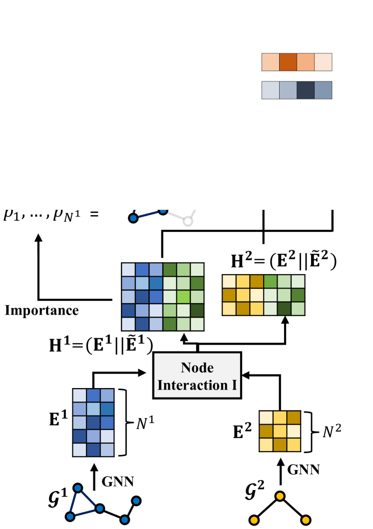
where $\mathbf{E}^{1}\in\mathbb{R}^{N^{1}\times d}$ and $\mathbf{E}^{2}\in\mathbb{R}^{N^{2}\times d}$ are node embedding matrices for $\mathcal{G}^{1}$ and $\mathcal{G}^{2}$, respectively, and $N^{1}$ and $N^{2}$ denote the number of nodes in $\mathcal{G}^{1}$ and $\mathcal{G}^{2}$, respectively. Then, we model the node-wise interaction between $\mathcal{G}^{1}$ and $\mathcal{G}^{2}$ via an interaction map $\mathbf{I}\in\mathbb{R}^{N^{1}\times N^{2}}$ defined as $\mathbf{I}_{ij}=\mathsf{sim}(\mathbf{E}_{i}^{1},\mathbf{E}_{j}^{2})$, where $\mathsf{sim}(\cdot,\cdot)$ indicates the cosine similarity. Then, we compute the embedding matrices $\tilde{\mathbf{E}}^{1}\in\mathbb{R}^{N^{1}\times d}$ and $\tilde{\mathbf{E}}^{2}\in\mathbb{R}^{N^{2}\times d}$ each of which regards its paired graph, based on the interaction map as $\tilde{\mathbf{E}}^{1}=\mathbf{I}\cdot\mathbf{E}^{2}$, and $\tilde{\mathbf{E}}^{2}=\mathbf{I}^{\top}\cdot\mathbf{E}^{1}$, where $\cdot$ indicates matrix multiplication between two matrices. Thus, $\tilde{\mathbf{E}}^{1}$ is the node embedding matrix of $\mathcal{G}^{1}$ that captures the interaction of nodes in $\mathcal{G}^{1}$ with those in $\mathcal{G}^{2}$, and likewise for $\tilde{\mathbf{E}}^{2}$. Then, we generate the final node embedding matrix of $\mathcal{G}^{1}$, i.e., $\mathbf{H}^{1}$, by concatenating $\mathbf{E}^{1}$ and $\tilde{\mathbf{E}}^{1}$, i.e., $\mathbf{H}^{1}=(\mathbf{E}^{1}||\tilde{\mathbf{E}}^{1})\in\mathbb{R}^{N^{1}\times 2d}$. The final node embedding matrix for $\mathcal{G}^{2}$, i.e., $\mathbf{H}^{2}$, is generated in a similar way. Lastly, we use Set2Set (Vinyals et al., 2015) as the graph readout function to generate the graph level embedding $\mathbf{z}_{\mathcal{G}^{1}}$ and $\mathbf{z}_{\mathcal{G}^{2}}$ for each graph $\mathcal{G}^{1}$ and $\mathcal{G}^{2}$, respectively. The overall model architecture is depicted in Figure 2.

4.3 Model Optimization

To train the model while simultaneously detecting the core subgraph, we optimize the model with the objective function defined in Equation 5 as follows:

$$\min\underbrace{-I(\mathbf{Y};\mathcal{G}_{\mathrm{CIB}}^{1}|\mathcal{G}^{2})}_{\text{Section \ref{sec:cond}}}+\beta\underbrace{I(\mathcal{G}^{1};\mathcal{G}_{\mathrm{CIB}}^{1}|\mathcal{G}^{2})}_{\text{Section \ref{sec:compression}}},$$ (8)

where each term indicates the prediction and compression, respectively. In the following sections, we provide the upper bound of each term, which should be minimized during training.

4.3.1 Minimizing $-I(\mathbf{Y};\mathcal{G}_{\mathrm{CIB}}^{1}|\mathcal{G}^{2})$

Following the chain rule of mutual information, the first term $-I(\mathbf{Y};\mathcal{G}_{\mathrm{CIB}}^{1}|\mathcal{G}^{2})$, which aims to keep task-relevant information in $\mathcal{G}_{\mathrm{CIB}}^{1}$ conditioned on $\mathcal{G}^{2}$, can be decomposed as follows:

$$-I(\mathbf{Y};\mathcal{G}_{\mathrm{CIB}}^{1}|\mathcal{G}^{2})=-I(\mathbf{Y};\mathcal{G}_{\mathrm{CIB}}^{1},\mathcal{G}^{2})+I(\mathbf{Y};\mathcal{G}^{2}).$$ (9)

However, we empirically find out that minimizing $I(\mathbf{Y};\mathcal{G}^{2})$ deteriorates the model performance (See Appendix C.5). Thus, we only consider $-I(\mathbf{Y};\mathcal{G}_{\mathrm{CIB}}^{1},\mathcal{G}^{2})$ in this work.

Proposition 4.4.

(Upper bound of $-I(\mathbf{Y};\mathcal{G}_{\mathrm{CIB}}^{1},\mathcal{G}^{2})$) Given a pair of graph $(\mathcal{G}^{1},\mathcal{G}^{2})$, its label information $\mathbf{Y}$, and the learned CIB-graph $\mathcal{G}_{CIB}^{1}$, we have

$$-I(\mathbf{Y};\mathcal{G}_{\mathrm{CIB}}^{1},\mathcal{G}^{2})\leq\mathbb{E}_{\mathcal{G}_{\mathrm{CIB}}^{1},\mathcal{G}^{2},\mathbf{Y}}{[-\log{p_{\theta}(\mathbf{Y}|\mathcal{G}_{\mathrm{CIB}}^{1},\mathcal{G}^{2})}]}$$ (10)

where $p_{\theta}(\mathbf{Y}|\mathcal{G}_{\mathrm{CIB}}^{1},\mathcal{G}^{2})$ is variational approximation of $p(\mathbf{Y}|\mathcal{G}_{\mathrm{CIB}}^{1},\mathcal{G}^{2})$.

We model $p_{\theta}(\mathbf{Y}|\mathcal{G}_{\mathrm{CIB}}^{1},\mathcal{G}^{2})$ as a predictor parametrized by $\theta$, which outputs the model prediction $\mathbf{Y}$ based on the input pair $(\mathcal{G}_{\mathrm{CIB}}^{1},\mathcal{G}^{2})$. Thus, we can minimize the upper bound of $-I(\mathbf{Y};\mathcal{G}_{\mathrm{\mathrm{CIB}}}^{1},\mathcal{G}^{2})$ by minimizing the model prediction loss $\mathcal{L}_{\mathrm{pred}}(\mathbf{Y},\mathcal{G}_{\mathrm{CIB}}^{1},\mathcal{G}^{2})$, which can be modeled as the cross entropy loss for classification and the mean square loss for regression. A detailed proof for proposition 10 is given in Appendix A.2.

4.3.2 Minimizing $I(\mathcal{G}^{1};\mathcal{G}_{\mathrm{CIB}}^{1}|\mathcal{G}^{2})$

For the second term of Equation 8, i.e., $I(\mathcal{G}^{1};\mathcal{G}_{\mathrm{CIB}}^{1}|\mathcal{G}^{2})$, we decompose the term into the sum of two terms based on the chain rule of mutual information as follows:

$$I(\mathcal{G}^{1};\mathcal{G}_{\mathrm{CIB}}^{1}|\mathcal{G}^{2})=I(\mathcal{G}_{\mathrm{CIB}}^{1};\mathcal{G}^{1},\mathcal{G}^{2})-I(\mathcal{G}_{\mathrm{CIB}}^{1};\mathcal{G}^{2}).$$ (11)

Intuitively, minimizing $I(\mathcal{G}_{\mathrm{CIB}}^{1};\mathcal{G}^{1},\mathcal{G}^{2})$ aims to compress the information of a pair of graph $(\mathcal{G}^{1},\mathcal{G}^{2})$ into $\mathcal{G}_{\mathrm{CIB}}^{1}$, while maximizing $I(\mathcal{G}_{\mathrm{CIB}}^{1};\mathcal{G}^{2})$ encourages $\mathcal{G}_{\mathrm{CIB}}^{1}$ to keep the information about a paired graph $\mathcal{G}^{2}$ during compression.

Minimizing $I(\mathcal{G}_{\mathrm{CIB}}^{1};\mathcal{G}^{1},\mathcal{G}^{2})$. Inspired by a recent approach on graph information bottleneck (Yu et al., 2022) that minimizes $I(\mathcal{G}_{\mathrm{IB}};\mathcal{G})$ by injecting noise into node representations, we compress the information contained in $\mathcal{G}^{1}$ and $\mathcal{G}^{2}$ into $\mathcal{G}^{1}_{\mathrm{CIB}}$ by injecting noise into the learned node representation $\mathbf{H}^{1}$ that contains information regarding both $\mathcal{G}^{1}$ and $\mathcal{G}^{2}$. The key idea is to enable the model to inject noise into insignificant subgraphs, while injecting less noise into more informative ones. More precisely, given a node $i$’s embedding $\mathbf{H}_{i}^{1}$, we calculate the probability $p_{i}$ with MLP, i.e., $p_{i}=\text{MLP}(\mathbf{H}_{i}^{1})$. With the calculated probability $p_{i}$, we replace the representation $\mathbf{H}_{i}^{1}$ of node $i$ with noise $\epsilon$, i.e., $\mathbf{T}_{i}^{1}=\lambda_{i}\mathbf{H}_{i}^{1}+(1-\lambda_{i})\epsilon$, where $\lambda_{i}\sim\text{Bernoulli}(\text{Sigmoid}(p_{i}))$ and $\epsilon\sim N(\mu_{\mathbf{H}^{1}},\sigma_{\mathbf{H}^{1}}^{2})$. Note that $\mu_{\mathbf{H}^{1}}$ and $\sigma_{\mathbf{H}^{1}}^{2}$ are mean and variance of $\mathbf{H}^{1}$, respectively. Thus, the information of $\mathcal{G}^{1}$ and $\mathcal{G}^{2}$ are compressed into $\mathcal{G}_{\text{CIB}}^{1}$ with the probability of $p_{i}$ by replacing non-important nodes with noise. That is, $p_{i}$ controls the information flow of $\mathcal{G}^{1}$ and $\mathcal{G}^{2}$ into $\mathcal{G}_{\text{CIB}}^{1}$. Moreover, to make the sampling process differentiable, we adopt gumbel sigmoid (Maddison et al., 2016; Jang et al., 2016) for discrete random variable $\lambda_{i}$, i.e., $\lambda_{i}=\text{Sigmoid}(1/t\log[{p_{i}/(1-p_{i})}]+\log{[u/(1-u)]})$ where $u\sim\text{Uniform}(0,1)$, and $t$ is the temperature hyperparameter. Finally, we minimize the upper bound of $I(\mathcal{G}_{\mathrm{CIB}}^{1};\mathcal{G}^{1},\mathcal{G}^{2})$ as follows:

$$\begin{split}I(\mathcal{G}_{\mathrm{CIB}}^{1};\mathcal{G}^{1},\mathcal{G}^{2})&\leq\mathbb{E}_{\mathcal{G}^{1},\mathcal{G}^{2}}{[-\frac{1}{2}\log A+\frac{1}{2N^{1}}A+\frac{1}{2N^{1}}B^{2}]}\\ &\coloneqq\mathcal{L}_{\mathrm{MI}^{1}}(\mathcal{G}_{\mathrm{CIB}}^{1},\mathcal{G}^{1},\mathcal{G}^{2})\end{split}$$ (12)

where $A=\sum_{j=1}^{N^{1}}{(1-\lambda_{j})^{2}}$ and $B=\frac{\sum_{j=1}^{N^{1}}{\lambda_{j}(\mathbf{H}_{j}^{1}-\mu_{\mathbf{H}^{1}})}}{\sigma_{\mathbf{H}^{1}}}$. A detailed proof for Equation 12 is given in Appendix A.3.

Minimizing $-I(\mathcal{G}_{\mathrm{CIB}}^{1};\mathcal{G}^{2})$. In this section, we introduce two different approaches for minimizing $-I(\mathcal{G}_{\mathrm{CIB}}^{1};\mathcal{G}^{2})$.

1) Variational IB-based approach. For the upper bound of $-I(\mathcal{G}_{\mathrm{CIB}}^{1};\mathcal{G}^{2})$, we adopt the variational IB-based approach (Alemi et al., 2016) as follows:

$$\small\begin{split}-I(\mathcal{G}_{\mathrm{CIB}}^{1};\mathcal{G}^{2})&\leq\mathbb{E}_{\mathcal{G}_{\mathrm{CIB}}^{1},\mathcal{G}^{2}}[-\log p_{\xi}(\mathcal{G}^{2}|\mathcal{G}_{\mathrm{CIB}}^{1})]\\ &\coloneqq\mathcal{L}_{\mathrm{MI}^{2}}(\mathcal{G}_{\mathrm{CIB}}^{1},\mathcal{G}^{2})\end{split}$$ (13)

where $p_{\xi}(\mathcal{G}^{2}|\mathcal{G}_{\mathrm{CIB}}^{1})$ is the variational approximation of $p(\mathcal{G}^{2}|\mathcal{G}_{\mathrm{CIB}}^{1})$. Although there exist various modeling choices for $p_{\xi}$ such as an MLP with non-linearity, we use a single-layered linear transformation without non-linearity. We argue that as more learnable parameters are involved in $p_{\xi}$, information that is useful for predicting $\mathcal{G}^{2}$ would be included in the parameters of $p_{\xi}$ rather than in the representation of $\mathcal{G}_{\mathrm{CIB}}^{1}$ itself, which incurs information loss as our goal is to obtain a high-quality representation of $\mathcal{G}_{\mathrm{CIB}}^{1}$. We indeed show in Appendix C.6 that a shallow $p_{\xi}$ is superior to a deep $p_{\xi}$.

2) Contrastive learning-based approach. Besides, recently proposed contrastive learning (Tian et al., 2020; Hjelm et al., 2018; You et al., 2020; Veličković et al., 2018), which learns to pull/push positive/negative samples in the representation space, has been theoretically proven to maximize the mutual information between positive pairs. Thus, we additionally propose a variant of CGIB, called $\textsf{CGIB}_{\textrm{cont}}$, which minimizes the term $-I(\mathcal{G}_{\mathrm{CIB}}^{1};\mathcal{G}^{2})$ by minimizing the contrastive loss rather than the upper bound defined in Equation 13 as follows:

$$\mathcal{L}_{\mathrm{MI}^{2}}=-\frac{1}{K}\sum_{i=1}^{K}\log\frac{\exp(\mathsf{sim}(\mathbf{z}_{\mathcal{G}_{\mathrm{CIB},i}^{1}},\mathbf{z}_{\mathcal{G}_{i}^{2}})/\tau)}{\sum_{j=1,j\neq i}^{K}{\exp(\mathsf{sim}(\mathbf{z}_{\mathcal{G}_{\mathrm{CIB},i}^{1}},\mathbf{z}_{\mathcal{G}_{j}^{2}})/\tau)}}$$ (14)

where $K$ and $\tau$ indicate the number of paired graphs in a batch and the temperature hyperparameter, respectively.

We argue that preserving the information of $\mathcal{G}^{2}$ in $\mathcal{G}_{\mathrm{CIB}}^{1}$ by minimizing $-I(\mathcal{G}_{\mathrm{CIB}}^{1};\mathcal{G}^{2})$ is the key to success of CGIB, which enables the conditional information compression of CGIB. We later demonstrate its importance in Section 5.3.2.

Final Objectives. Finally, we train the model with the final objective given as follows:

$$\mathcal{L}_{\mathrm{total}}=\mathcal{L}_{\mathrm{sup}}+{\mathcal{L}_{\mathrm{pred}}}+\beta({\mathcal{L}_{\mathrm{MI}^{1}}}+{\mathcal{L}_{\mathrm{MI}^{2}}})$$ (15)

where $\beta$ controls the trade-off between prediction and compression. Note that the supervised loss, i.e., $\mathcal{L}_{\mathrm{sup}}$, calculates the loss between the model prediction given the pair of input graphs, i.e., $(\mathcal{G}^{1}$, $\mathcal{G}^{2})$, and the target response, i.e., $\mathbf{Y}$, without detecting the core subgraphs. Moreover, in Appendix C.2, we conduct analyses on the selection of $\mathcal{G}^{1}$ and $\mathcal{G}^{2}$, and provide a guidance regarding how to decide which one of the graphs to use as $\mathcal{G}^{1}$.

5 Experiments

5.1 Experimental Setup

Datasets. We use eleven datasets to comprehensively evaluate the performance of CGIB  on three tasks, i.e., 1) molecular interaction prediction, 2) drug-drug interaction (DDI) prediction, and 3) graph similarity learning. Specifically, for the molecular interaction prediction task, we use Chromophore dataset (Joung et al., 2020), which is related to three optical properties of chromophores, as well as 5 other datasets, i.e., MNSol (Marenich et al., 2020), FreeSolv (Mobley & Guthrie, 2014), CompSol (Moine et al., 2017), Abraham (Grubbs et al., 2010), and CombiSolv (Vermeire & Green, 2021), which are related to the solvation free energy of solute. In Chromophore dataset, maximum absorption wavelength (Absorption), maximum emission wavelength (Emission) and excited state lifetime (Lifetime) properties are used in this work. For the DDI prediction task, we use 2 datasets, i.e., ZhangDDI (Zhang et al., 2017) and ChChMiner (Zitnik et al., 2018), both of which contain labeled DDI data. Lastly, for the graph similarity learning task, we use 3 datasets, i.e., AIDS, IMDB (Bai et al., 2019), and OpenSSL (Xu et al., 2017), each of which is related to chemical compound, ego-network, and binary function’s control flow, respectively. Further details on datasets are described in Appendix B.

Methods Compared. For all three tasks, we compare CGIB with the state-of-the-art methods. Specifically, for the molecular interaction prediction task, we mainly compare with CIGIN (Pathak et al., 2020). For the DDI prediction task, we mainly compare with SSI-DDI (Nyamabo et al., 2021) and MIRACLE (Wang et al., 2021), and additionally compare with CIGIN (Pathak et al., 2020) by changing its prediction head originally designed for regression to classification. Note that for the molecular interaction and DDI prediction tasks, we also compare CGIB with simple baseline methods, i.e., GCN (Kipf & Welling, 2016), GAT (Veličković et al., 2017), MPNN (Gilmer et al., 2017), and GIN (Xu et al., 2018). Specifically, we independently encode a pair of graphs based on Set2Set pooling for fair comparisons, and concatenate the two encoded vectors to predict the target value by using an MLP. Further details regarding the compared methods for the graph similarity learning task are described in Appendix C.1.

Table 1: Performance on molecular interaction prediction task (regression) in terms of RMSE.

Model		Chromophore				MNSol	FreeSolv	CompSol	Abraham	CombiSolv
		Absorption	Emission	Lifetime
Interaction ✗
GCN		$25.75$ (1.48)	$31.87$ (1.70)	$0.866$ (0.015)		$0.675$ (0.021)	$1.192$ (0.042)	$0.389$ (0.009)	$0.738$ (0.041)	$0.672$ (0.022)
GAT		$26.19$ (1.44)	$30.90$ (1.01)	$0.859$ (0.016)		$0.731$ (0.007)	$1.280$ (0.049)	$0.387$ (0.010)	$0.798$ (0.038)	$0.662$ (0.021)
MPNN		$24.43$ (1.55)	$30.17$ (0.99)	$0.802$ (0.024)		$0.682$ (0.017)	$1.159$ (0.032)	$0.359$ (0.011)	$0.601$ (0.035)	$0.568$ (0.005)
GIN		$24.92$ (1.67)	$32.31$ (0.26)	$0.829$ (0.027)		$0.669$ (0.017)	$1.015$ (0.041)	$0.331$ (0.016)	$0.648$ (0.024)	$0.595$ (0.014)
Interaction ✓
CIGIN		$19.32$ (0.35)	$25.09$ (0.32)	$0.804$ (0.010)		$0.607$ (0.024)	$0.905$ (0.014)	$0.308$ (0.018)	$0.411$ (0.008)	$0.451$ (0.009)
CGIB		$\mathbf{17.87}$ (0.38)	$24.44$ (0.21)	$0.796$ (0.010)		$0.568$ (0.013)	$\mathbf{0.831}$(0.012)	$0.277$ (0.008)	$0.396$ (0.009)	$0.428$ (0.009)
$\textsf{CGIB}_{\textrm{cont}}$		$18.11$ (0.20)	$\mathbf{23.90}$ (0.35)	$\mathbf{0.771}$ (0.005)		$\mathbf{0.538}$ (0.007)	$0.852$ (0.022)	$\mathbf{0.276}$ (0.017)	$\mathbf{0.390}$ (0.006)	$\mathbf{0.422}$ (0.005)

Table 2: Performance on drug-drug interaction prediction task (classification).

Model		(a) Transductive						(b) Inductive
		ZhangDDI			ChChMiner			ZhangDDI			ChChMiner
		AUROC	Accuracy		AUROC	Accuracy		AUROC	Accuracy		AUROC	Accuracy
Interaction ✗
GCN		$91.64$ (0.31)	$83.31$ (0.61)		$94.71$ (0.33)	$87.36$ (0.24)		$68.39$ (1.85)	$63.78$ (1.55)		$73.63$ (0.44)	$67.07$ (0.66)
GAT		$92.10$ (0.28)	$84.14$ (0.38)		$96.15$ (0.53)	$89.49$ (0.88)		$69.99$ (2.95)	$64.41$ (1.39)		$75.72$ (1.66)	$68.77$ (1.48)
MPNN		$92.34$ (0.35)	$84.56$ (0.31)		$96.25$ (0.53)	$90.02$ (0.42)		$71.54$ (1.24)	$65.12$ (1.14)		$75.45$ (0.32)	$68.24$ (1.42)
GIN		$93.16$ (0.04)	$85.59$ (0.05)		$97.52$ (0.05)	$91.89$ (0.66)		$72.74$ (1.32)	$66.16$ (1.21)		$74.63$ (0.48)	$67.80$ (0.46)
Interaction ✓
SSI-DDI		$92.74$ (0.12)	$84.61$ (0.18)		$98.44$ (0.08)	$93.50$ (0.16)		$73.29$ (2.23)	$66.53$ (1.31)		$78.24$ (1.29)	$70.69$ (1.47)
MIRACLE		$93.05$ (0.07)	$84.90$ (0.36)		$88.66$ (0.37)	$84.29$ (0.14)		$73.23$ (3.32)	$50.00$ (0.00)		$60.25$ (0.56)	$50.09$ (0.11)
CIGIN		$93.28$ (0.13)	$85.54$ (0.30)		$98.51$ (0.10)	$93.77$ (0.25)		$74.02$ (0.10)	$66.81$ (0.09)		$79.23$ (0.51)	$71.56$ (0.38)
CGIB		$\mathbf{94.74}$ (0.47)	$\mathbf{86.88}$ (0.56)		$98.80$ (0.04)	$\mathbf{94.69}$ (0.16)		$74.59$ (0.88)	$\mathbf{67.65}$ (1.07)		$81.14$ (1.20)	$72.47$ (0.16)
$\textsf{CGIB}_{\textrm{cont}}$		$93.78$ (0.62)	$86.36$ (0.75)		$\mathbf{98.84}$ (0.31)	$94.52$ (0.38)		$\mathbf{75.08}$ (0.34)	$67.31$ (0.82)		$\mathbf{81.51}$ (0.67)	$\mathbf{74.29}$ (0.14)

Evaluation Metrics. The performance of the molecular interaction prediction task is evaluated in terms of RMSE (Pathak et al., 2020), that of the drug-drug interaction prediction task is evaluated in terms of AUROC and accuracy (Wang et al., 2021), and that of similarity learning task is evaluated in terms of MSE, Spearman’s Rank Correlation Coefficient (denoted as $\rho$), and precision@10 (p@10) (Zhang et al., 2021). We further provide the details on the evaluation protocol in Appendix D.

Implementation Details. For the molecular interaction prediction and graph similarity learning tasks, we use 3-layer MPNN (Gilmer et al., 2017) and GCN (Kipf & Welling, 2016) as our backbone graph encoder, respectively, and a 3-layer MLP with ReLU activation as the predictor following the previous works (Pathak et al., 2020; Zhang et al., 2021). For the drug-drug interaction prediction task, we use GIN (Xu et al., 2018) as our backbone graph encoder, and a single layer MLP without activation as the predictor. Hyperparameter details are described in Appendix E.

Figure 3: Model analysis.

5.2 Overall Performance

The empirical performance of CGIB on molecular interaction prediction and drug-drug interaction prediction tasks is summarized in Table 1 and Table 2, respectively. We have the following observations: 1) CGIB outperforms all other baseline methods that overlook the significance of the core subgraph during training in both molecular interaction prediction task (i.e., CIGIN), and drug-drug interaction prediction task (SSI-DDI and MIRACLE). We argue that CGIB improves its generalization ability by making predictions based on the detected core subgraph of the given graph, which is the minimal structure sufficient to represent the properties of the graph. Considering that a certain functional group induces the same or similar chemical reactions, learning from the core substructure is crucial, especially in chemical reaction prediction tasks. 2) To further demonstrate the generalization ability of CGIB, we conduct additional experiments in the inductive setting (Table 2(b)), which is more practical and closer to the real-world applications. We observe that CGIB consistently outperforms other baseline methods in the inductive setting as well, which verifies the practicality of CGIB. We argue that as CGIB makes predictions based on the core subgraphs of graphs that are shared among the total set of graphs, i.e., $\mathbb{G}$ (Refer to Appendix D), CGIB can make accurate predictions even though the graphs in the test set are not seen during training. Based on the results of these two experiments, we argue that the key to the success of CGIB is the generalization ability thanks to the detection of the core subgraph during training. 3) It is worth noting that simple baseline methods that naively concatenate the representations of a pair of graphs, i.e., GCN, GAT, MPNN, and GIN, generally perform worse than the methods that consider the interaction between the graphs, i.e., CIGIN, SSI-DDI, and MIRACLE, which implies that modeling the interaction between graphs is important in relational learning framework. To verify the wide applicability of CGIB, we conduct experiments on the graph similarity learning task in Appendix C.1.

5.3 Model Analysis

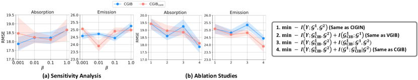
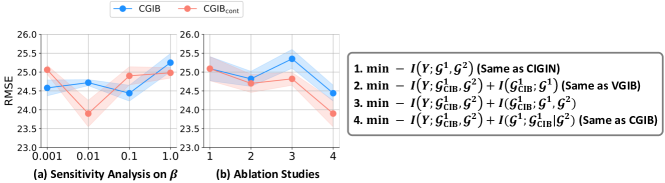
5.3.1 Sensitivity Analysis on $\beta$

In this section, we analyze the effect of $\beta$, which controls the trade-off between the prediction and compression in our final objectives shown in Equation 15. As shown in Figure 3 (a), there exists the optimal point of $\beta$ in terms of the model performance, which indicates the existence of the trade-off between the prediction and the information compression. We have the following observations: 1) The model consistently performs the worst when $\beta=1$. This is because $\beta=1$ encourages the model to aggressively compress the information of the input graph, thereby hardly capturing the core subgraph that is related to the target task. 2) On the other hand, decreasing $\beta$ does not always lead to a good performance. Recall that decreasing $\beta$ encourages the model to keep the original information of the given graph structure. In an extreme case, i.e., when $\beta=0$, the model would not consider the information compression at all. In this case, since the model only needs to focus on the prediction term, prediction can be made using the entire graph structure without finding the core subgraph, which consequently leads to the lack of the generalization ability. Recent works on augmentation (Gontijo-Lopes et al., 2020; Zhu et al., 2021) can also shed light on this phenomenon, i.e., $\beta$ controls the trade-off between affinity and diversity. We also conduct qualitative analysis on $\beta$ in Appendix C.7.

5.3.2 Ablation Studies

To verify the benefit of the conditional compression module of CGIB, i.e., ${I(\mathcal{G}^{1};\mathcal{G}_{\mathrm{CIB}}^{1}|\mathcal{G}^{2})}$ described in Section 4.3.2, we conduct ablation studies on two datasets, i.e., Absorption and Emission, in Figure 3 (b). Recall that the conditional mutual information $I(\mathcal{G}^{1};\mathcal{G}^{1}_{\mathrm{CIB}}|\mathcal{G}^{2})$ is decomposed as shown in Equation 11: $I(\mathcal{G}^{1};\mathcal{G}^{1}_{\mathrm{CIB}}|\mathcal{G}^{2})=I(\mathcal{G}^{1}_{\mathrm{CIB}};\mathcal{G}^{1},\mathcal{G}^{2})-I(\mathcal{G}^{1}_{\mathrm{CIB}};\mathcal{G}^{2})$. We have the following observations: 1) Existing methods that only take a single graph into account (i.e., $I(\mathcal{G}^{1}_{\mathrm{CIB}};\mathcal{G}^{1})$), also perform better than the baseline that does not consider the subgraph at all (i.e., Without IB). This implies that considering the core subgraph of the given graph generally improves the model performance. 2) On the other hand, given two graphs $\mathcal{G}^{1}$ and $\mathcal{G}^{2}$, compressing the information by minimizing the conditional mutual information (i.e., $I(\mathcal{G}^{1};\mathcal{G}^{1}_{\mathrm{CIB}}|\mathcal{G}^{2})$) instead of the joint mutual information (i.e., $I(\mathcal{G}^{1}_{\mathrm{CIB}};\mathcal{G}^{1},\mathcal{G}^{2})$) is crucial in relational learning. This is because the conditional mutual information encourages the compressed subgraph $\mathcal{G}^{1}_{\mathrm{CIB}}$ of graph $\mathcal{G}^{1}$ to keep the information regarding $\mathcal{G}^{2}$, due to the additional $I(\mathcal{G}_{\text{CIB}}^{1};\mathcal{G}^{2})$ maximization term that appears in the decomposition of $I(\mathcal{G}^{1};\mathcal{G}^{1}_{\mathrm{CIB}}|\mathcal{G}^{2})$. That is, by assuring $\mathcal{G}^{1}_{\mathrm{CIB}}$ to have information about $\mathcal{G}^{2}$, the model considers $\mathcal{G}^{2}$ during the compression procedure, which aligns with our conditional information bottleneck objective. 3) Moreover, compressing the information by minimizing the conditional mutual information consistently outperforms compressing the information solely based on a single graph, i.e., $I(\mathcal{G}^{1}_{\mathrm{CIB}};\mathcal{G}^{1})$, which is equivalent to VGIB (Yu et al., 2022). This is because the core subgraph of $\mathcal{G}^{1}$ should be determined based on the other graph to be interacted with, i.e., $\mathcal{G}^{2}$. Therefore, we argue that the current graph information bottleneck approaches such as VGIB (Yu et al., 2022), GIB (Yu et al., 2020), and GSAT (Miao et al., 2022), are not suitable for relational learning tasks. 4) What’s interesting is that naively modeling the joint compression simply through the joint mutual information (i.e., $I(\mathcal{G}^{1}_{\mathrm{CIB}};\mathcal{G}^{1},\mathcal{G}^{2})$) performs even worse than considering only single graph (i.e., $I(\mathcal{G}^{1}_{\mathrm{CIB}};\mathcal{G}^{1})$). This implies that if the compressed subgraph $\mathcal{G}^{1}_{\mathrm{CIB}}$ does not fully contain the information of $\mathcal{G}^{2}$, the information of $\mathcal{G}^{2}$ can interfere with the optimal compression of the pair ($\mathcal{G}^{1}$, $\mathcal{G}^{2}$) into $\mathcal{G}^{1}_{\mathrm{CIB}}$. Due to the suboptimality, the model trained with the joint mutual information sometimes performs worse than the one that does not consider the subgraph at all (i.e., Without IB).

To summarize our findings, the ablation studies demonstrate that simply adopting IB principle into relational learning framework is not trivial, and that CGIB successfully adopts the IB principle for relational learning.

Figure 4: Qualitative analysis on CIB-Graph.

5.4 Qualitative Analysis on CIB-Graph

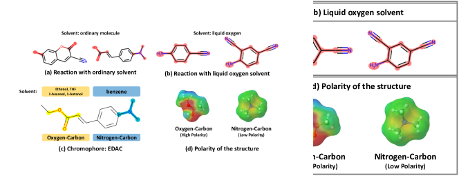
We qualitatively analyze the substructures based on our prior chemical knowledge. In the Chromophore dataset, CGIB predicts that the edge substructures of chromophores are important in the chromophore-solvent reactions, as shown in Figure 4(a). This prediction result of CGIB  aligns with the chemical knowledge that chemical reactions usually happen around the ionized atoms (Hynes, 1985). Figure 4(b) shows the important substructures of chromophores predicted by CGIB when they react with liquid oxygen solvents. As shown in the results, CGIB predicts that the entire structure is important in the chemical reactions between chromophores and oxygen solvents. This result again aligns with the chemical knowledge that chemical reactions can happen in the entire molecule because the size of the oxygen solvent is small enough to permeate the chromophores.

We also find out that the important substructure of chromophores predicted by CGIB varies according to which solvent the chromophores react with. Figure 4(c) shows the important substructure in a chromophore named trans-ethyl p-(dimethylamino) cinamate (EDAC) (Singh et al., 2009) detected by CGIB in five different solvents: benzene, ethanol, THF, 1-hexanol, and 1-butanol. We observe that CGIB predicts that the nitrogen-carbon substructure (marked in blue) is important in the benzene solvent, whereas the oxygen-carbon substructure (marked in yellow) is predicted to be important in the ethanol, THF, 1-hexanol, and 1-butanol solvents. These results can be understood by the chemical polarity and the solvent solubility. Since nonpolar molecules usually interact with nonpolar molecules (Reichardt, 1965), the low-polarity nitrogen-carbon substructure is considered as an important substructure in benzene, which is a completely nonpolar solvent. On the other hand, polar molecules interact with polar molecules. Hence, the oxygen-carbon substructure with polarity is considered as an important substructure in the polar solvents ethanol and THF, all of which are polar solvents. Note that the polarity of nitrogen-carbon substructure and oxygen-carbon structure is denoted in Figure 4 (d) left and right, respectively. Although 1-hexanol and 1-butanol are categorized into nonpolar solvents due to their overall weak polarity, the OH substructures in 1-hexanol and 1-butanol have a local polarity. For this reason, we conjecture that the oxygen-carbon substructure is predicted to be important in 1-hexanol and 1-butanol solvents. We further provide a quantitative analysis on the selected CIB-Graph, i.e., $\mathcal{G}^{1}_{\text{CIB}}$ in Appendix C.4.

6 Conclusion

In this paper, we propose a novel molecular relational learning framework, named CGIB, which predicts the interaction behavior between a pair of molecules by detecting important subgraphs therein. The main idea is, given a pair of molecules, to find a substructure of a given molecule containing the minimal sufficient information regarding the task at hand conditioned on the paired molecule based on the principle of conditional graph information bottleneck. By doing so, CGIB adaptively selects the core substructure of the input molecule according to its paired molecule, which aligns with the nature of chemical reactions. Our extensive experiments demonstrate that CGIB consistently outperforms existing state-of-the-art methods in molecular relational learning tasks. Moreover, CGIB provides convincing explanations regarding chemical reactions, which verifies its practicality in real-world applications.

Acknowledgement This work was supported by Institute of Information & communications Technology Planning & Evaluation (IITP) grant funded by the Korea government(MSIT) (No.2022-0-00077), and core KRICT project from the Korea Research Institute of Chemical Technology (KK2351-10).

Appendix A Proofs

A.1 Proof of Lemma 4.3

Assuming that $\mathcal{G}^{1},\mathcal{G}_{\mathrm{CIB}}^{1},\mathcal{G}_{n}^{1},\mathcal{G}^{2},$ and $\mathbf{Y}$ satisfy the markov condition $(\mathbf{Y},\mathcal{G}_{n}^{1},\mathcal{G}^{2})\rightarrow\mathcal{G}^{1}\rightarrow\mathcal{G}_{\mathrm{CIB}}^{1}$, we have the following inequality due to data processing inequality:

$$\small\begin{split}I(\mathcal{G}^{1};\mathcal{G}_{\mathrm{CIB}}^{1}|\mathcal{G}^{2})&=I(\mathcal{G}_{\mathrm{CIB}}^{1};\mathcal{G}^{1},\mathcal{G}^{2})-I(\mathcal{G}_{\mathrm{CIB}}^{1};\mathcal{G}^{2})\\ &\geq I(\mathcal{G}_{\mathrm{CIB}}^{1};\mathbf{Y},\mathcal{G}_{n}^{1},\mathcal{G}^{2})-I(\mathcal{G}_{\mathrm{CIB}}^{1};\mathcal{G}^{2})\\ &=I(\mathcal{G}_{\mathrm{CIB}}^{1};\mathcal{G}_{n}^{1},\mathcal{G}^{2})+I(\mathcal{G}_{\mathrm{CIB}}^{1};\mathbf{Y}|\mathcal{G}_{n}^{1},\mathcal{G}^{2})-I(\mathcal{G}_{\mathrm{CIB}}^{1};\mathcal{G}^{2})\\ &=I(\mathcal{G}_{\mathrm{CIB}}^{1};\mathcal{G}_{n}^{1}|\mathcal{G}^{2})+I(\mathcal{G}_{\mathrm{CIB}}^{1};\mathbf{Y}|\mathcal{G}_{n}^{1},\mathcal{G}^{2})\end{split}$$ (16)

Suppose that $\mathcal{G}_{n}^{1}$ and $\mathbf{Y}$, $\mathcal{G}_{n}^{1}$ and $\mathcal{G}^{2}$, and joint random variable $(\mathcal{G}_{n}^{1},\mathcal{G}^{2})$ and $\mathbf{Y}$ are independent, respectively. Then, for $I(\mathcal{G}_{\mathrm{CIB}}^{1};\mathbf{Y}|\mathcal{G}_{n}^{1},\mathcal{G}^{2})$, we have:

$$\small\begin{split}I(\mathcal{G}_{\mathrm{CIB}}^{1};\mathbf{Y}|\mathcal{G}_{n}^{1},\mathcal{G}^{2})&=H(\mathbf{Y}|\mathcal{G}_{n}^{1},\mathcal{G}^{2})-H(\mathbf{Y}|\mathcal{G}_{n}^{1},\mathcal{G}_{\mathrm{CIB}}^{1},\mathcal{G}^{2})\\ &\geq H(\mathbf{Y}|\mathcal{G}^{2})-H(\mathbf{Y}|\mathcal{G}_{\mathrm{CIB}}^{1},\mathcal{G}^{2})\\ &=I(\mathbf{Y};\mathcal{G}_{\mathrm{CIB}}^{1}|\mathcal{G}^{2})\end{split}$$ (17)

By plugging Equation 17 into Equation 16, we have:

$$\small I(\mathcal{G}^{1};\mathcal{G}_{\mathrm{CIB}}^{1}|\mathcal{G}^{2})\geq I(\mathcal{G}_{\mathrm{CIB}}^{1};\mathcal{G}_{n}^{1}|\mathcal{G}^{2})+I(\mathbf{Y};\mathcal{G}_{\mathrm{CIB}}^{1}|\mathcal{G}^{2})$$ (18)

A.2 Proof of Proposition 4.4

By the definition of mutual information and introducing variational approximation $p_{\theta}(\mathbf{Y}|\mathcal{G}_{CIB}^{1},\mathcal{G}^{2})$ of intractable distribution $p(\mathbf{Y}|\mathcal{G}_{CIB}^{1},\mathcal{G}^{2})$, we have:

$$\small\begin{split}I(\mathbf{Y};\mathcal{G}_{\mathrm{CIB}}^{1},\mathcal{G}^{2})&=\mathbb{E}_{\mathbf{Y},\mathcal{G}_{\mathrm{CIB}}^{1},\mathcal{G}^{2}}[\log\frac{p(\mathbf{Y}|\mathcal{G}_{\mathrm{CIB}}^{1},\mathcal{G}^{2})}{p(\mathbf{Y})}]\\ &=\mathbb{E}_{\mathbf{Y},\mathcal{G}_{\mathrm{CIB}}^{1},\mathcal{G}^{2}}[\log\frac{p_{\theta}(\mathbf{Y}|\mathcal{G}_{\mathrm{CIB}}^{1},\mathcal{G}^{2})}{p(\mathbf{Y})}]\\ &+\mathbb{E}_{\mathcal{G}_{\mathrm{CIB}}^{1},\mathcal{G}^{2}}[KL(p(\mathbf{Y}|\mathcal{G}_{\mathrm{CIB}}^{1},\mathcal{G}^{2})||p_{\theta}(\mathbf{Y}|\mathcal{G}_{\mathrm{CIB}}^{1},\mathcal{G}^{2}))]\\ \end{split}$$ (19)

According to the non-negativity of the KL divergence, we have:

$$\small\begin{split}I(\mathbf{Y};\mathcal{G}_{\mathrm{CIB}}^{1},\mathcal{G}^{2})&\geq\mathbb{E}_{\mathbf{Y},\mathcal{G}_{\mathrm{CIB}}^{1},\mathcal{G}^{2}}[\log\frac{p_{\theta}(\mathbf{Y}|\mathcal{G}_{\mathrm{CIB}}^{1},\mathcal{G}^{2})}{p(\mathbf{Y})}]\\ &=\mathbb{E}_{\mathbf{Y},\mathcal{G}_{\mathrm{CIB}}^{1},\mathcal{G}^{2}}[\log p_{\theta}(\mathbf{Y}|\mathcal{G}_{\mathrm{CIB}}^{1},\mathcal{G}^{2})]+H(\mathbf{Y})\\ \end{split}$$ (20)

A.3 Proof of Equation 12

Given the perturbed graph $\mathcal{G}_{\mathrm{CIB}}^{1}$ and its representation $\mathbf{z}_{\mathcal{G}_{\mathrm{CIB}}^{1}}$, we assume there is no information loss during the readout process, i.e., $I(\mathbf{z}_{\mathcal{G}_{\mathrm{CIB}}^{1}};\mathcal{G}^{1},\mathcal{G}^{2})\approx I(\mathcal{G}_{\mathrm{CIB}}^{1};\mathcal{G}^{1},\mathcal{G}^{2})$. Now, we derive the upper bound of $I(\mathbf{z}_{\mathcal{G}_{\mathrm{CIB}}^{1}};\mathcal{G}^{1},\mathcal{G}^{2})$ by introducing the variation approximation $q(\mathbf{z}_{\mathcal{G}_{\mathrm{CIB}}^{1}})$ of distribution $p(\mathbf{z}_{\mathcal{G}_{\mathrm{CIB}}^{1}})$:

$$\small\begin{split}I(\mathbf{z}_{\mathcal{G}_{\mathrm{CIB}}^{1}};\mathcal{G}^{1},\mathcal{G}^{2})&=\mathbb{E}_{\mathbf{z}_{\mathcal{G}_{\mathrm{CIB}}^{1}},\mathcal{G}^{1},\mathcal{G}^{2}}[\log\frac{p_{\phi}(\mathbf{z}_{\mathcal{G}_{\mathrm{CIB}}^{1}}|\mathcal{G}^{1},\mathcal{G}^{2})}{p(\mathbf{z}_{\mathcal{G}_{\mathrm{CIB}}^{1}})}]\\ &=\mathbb{E}_{\mathcal{G}^{1},\mathcal{G}^{2}}[\log\frac{p_{\phi}(\mathbf{z}_{\mathcal{G}_{\mathrm{CIB}}^{1}}|\mathcal{G}^{1},\mathcal{G}^{2})}{q(\mathbf{z}_{\mathcal{G}_{\mathrm{CIB}}^{1}})}]\\ &-\mathbb{E}_{\mathbf{z}_{\mathcal{G}_{\mathrm{CIB}}^{1}},\mathcal{G}^{1},\mathcal{G}^{2}}[KL(p(\mathbf{z}_{\mathcal{G}_{\mathrm{CIB}}^{1}})||q(\mathbf{z}_{\mathcal{G}_{\mathrm{CIB}}^{1}}))]\\ \end{split}$$ (21)

According to the non-negativity of KL divergence, we have:

$$\small I(\mathbf{z}_{\mathcal{G}_{\mathrm{CIB}}^{1}};\mathcal{G}^{1},\mathcal{G}^{2})\leq\mathbb{E}_{\mathcal{G}^{1},\mathcal{G}^{2}}[KL(p_{\phi}(\mathbf{z}_{\mathcal{G}_{\mathrm{CIB}}^{1}}|\mathcal{G}^{1},\mathcal{G}^{2})||q(\mathbf{z}_{\mathcal{G}_{\mathrm{CIB}}^{1}}))]$$ (22)

Following VIB (Alemi et al., 2016), we assume that $q(\mathbf{z}_{\mathcal{G}_{\mathrm{CIB}}^{1}})$ is obtained by aggregating the node representations in a fully perturbed graph. The noise $\epsilon\sim N(\mu_{\mathbf{H}^{1}},\sigma_{\mathbf{H}^{1}}^{2})$ is sampled from a Gaussian distribution where $\mu_{\mathbf{H}^{1}}$ and $\sigma_{\mathbf{H}^{1}}^{2}$ are mean and variance of $\mathbf{H}^{1}$ which contains information of both $\mathcal{G}^{1}$ and $\mathcal{G}^{2}$. Choosing sum pooling as the readout function, since the summation of Gaussian distributions is a Gaussian, we have the following equation:

$$\small q(\mathbf{z}_{\mathcal{G}_{\mathrm{CIB}}^{1}})=\mathcal{N}(N^{1}\mu_{\mathbf{H}^{1}},N^{1}\sigma_{\mathbf{H}^{1}}^{2})$$ (23)

Then for $p_{\phi}(\mathbf{z}_{\mathcal{G}_{\mathrm{CIB}}^{1}}|\mathcal{G}^{1},\mathcal{G}^{2})$, we have the following equation:

$$\small p_{\phi}(\mathbf{z}_{\mathcal{G}_{\mathrm{CIB}}^{1}}|\mathcal{G}^{1},\mathcal{G}^{2})=\mathcal{N}(N^{1}\mu_{\mathbf{H}^{1}}+\sum_{j=1}^{N^{1}}{\lambda_{j}\mathbf{H}_{j}^{1}}-\sum_{j=1}^{N^{1}}{\lambda_{j}\mu_{\mathbf{H}^{1}}},\sum_{j=1}^{N^{1}}{(1-\lambda_{j})^{2}\sigma_{\mathbf{H}^{1}}^{2}})$$ (24)

Finally, we have following inequality by plugging Equation 23 and Equation 24 into Equation Equation 22:

$$\small I(\mathbf{z}_{\mathcal{G}_{\mathrm{CIB}}^{1}};\mathcal{G}^{1},\mathcal{G}^{2})\leq\mathbb{E}_{\mathcal{G}^{1},\mathcal{G}^{2}}{[-\frac{1}{2}\log A+\frac{1}{2N^{1}}A+\frac{1}{2N^{1}}B^{2}]}+C$$ (25)

where $A=\sum_{j=1}^{N^{1}}{(1-\lambda_{j})^{2}}$, $B=\frac{\sum_{j=1}^{N^{1}}{\lambda_{j}(\mathbf{H}_{j}^{1}-\mu_{\mathbf{H}^{1}})}}{\sigma_{\mathbf{H}^{1}}}$ and $C$ is a constant term which is ignored during optimization.

Appendix B Datasets

In this section we provide details on the datasets used during training. The detailed statistics are summarized in Table 3

Molecular Interaction Prediction. For the datasets used in the molecular interaction prediction task, we convert the SMILES string into graph structure by using the Github code of CIGIN (Pathak et al., 2020). Moreover, for the datasets that are related to solvation free energies, i.e., MNSol, FreeSolv, CompSol, Abraham, and CombiSolv, we use the SMILES-based datasets provided in the previous work (Vermeire & Green, 2021). Only solvation free energies at temperatures of 298 K ($\pm$ 2) are considered and ionic liquids and ionic solutes are removed (Vermeire & Green, 2021).

• Chromophore (Joung et al., 2020) contains 20,236 combinations of 7,016 chromophores and 365 solvents which are given in the SMILES string format. All optical properties are based on scientific publications and unreliable experimental results are excluded after examination of absorption and emission spectra. In this dataset, we measure our model performance on predicting maximum absorption wavelength (Absorption), maximum emission wavelength (Emission) and excited state lifetime (Lifetime) properties which are important parameters for the design of chromophores for specific applications. We delete the NaN values to create each dataset which is not reported in the original scientific publications. Moreover, for Lifetime data, we use log normalized target value since the target value of the dataset is highly skewed inducing training instability.

• MNSol (Marenich et al., 2020) contains 3,037 experimental free energies of solvation or transfer energies of 790 unique solutes and 92 solvents. In this work, we consider 2,275 combinations of 372 unique solutes and 86 solvents following previous work (Vermeire & Green, 2021).

• FreeSolv (Mobley & Guthrie, 2014) provides 643 experimental and calculated hydration free energy of small molecules in water. In this work, we consider 560 experimental results following previous work (Vermeire & Green, 2021).

• CompSol (Moine et al., 2017) dataset is proposed to show how solvation energies are influenced by hydrogen-bonding association effects. We consider 3,548 combinations of 442 unique solutes and 259 solvents in the dataset following previous work (Vermeire & Green, 2021).

• Abraham (Grubbs et al., 2010) dataset is a collection of data published by the Abraham research group at College London. We consider 6,091 combinations of 1,038 unique solutes and 122 solvents following previous work (Vermeire & Green, 2021).

• CombiSolv (Vermeire & Green, 2021) contains all the data of MNSol, FreeSolv, CompSol, and Abraham, resulting in 10,145 combinations of 1,368 solutes and 291 solvents.

Drug-Drug Interaction Prediction. For the datasets used in the drug-drug interaction prediction task, we use the positive drug pairs given in MIRACLE Github link, which removed the data instances that cannot be converted into graphs from SMILES strings. Then, we generate negative counterparts by sampling a complement set of positive drug pairs as the negative set for both datasets. We also follow the graph converting process of MIRACLE (Wang et al., 2021) for classification task.

• ZhangDDI (Zhang et al., 2017) contains 548 drugs and 48,548 pairwise interaction data and multiple types of similarity information about these drug pairs.

• ChChMiner (Zitnik et al., 2018) contains 1,322 drugs and 48,514 labeled DDIs, obtained through drug labels and scientific publications.

Although ChChMiner dataset has much more drug instances than ZhangDDI dataset, the number of labeled DDI is almost the same. This indicates that ChChMiner dataset has much more sparse relationship between the drugs.

Table 3: Data statistics.

Task	Dataset		$\mathcal{G}^{1}$	$\mathcal{G}^{2}$	# $\mathcal{G}^{1}$	# $\mathcal{G}^{2}$	# Pairs
		Absorption	Chrom.	Solvent	6416	725	17276
	Chromophore	Emission	Chrom.	Solvent	6412	1021	18141
		Lifetime	Chrom.	Solvent	2755	247	6960
Molecular	MNSol		Solute	Solvent	372	86	2275
Interaction	FreeSolv		Solute	Solvent	560	1	560
	CompSol		Solute	Solvent	442	259	3548
	Abraham		Solute	Solvent	1038	122	6091
	CombiSolv		Solute	Solvent	1495	326	10145
Drug-Drug	ZhangDDI		Drug	Drug	544	544	40255
Interaction	ChChMiner		Drug	Drug	949	949	21082
Graph	AIDS		Mole.	Mole.	700	700	490K
Similarity	IMDB 11		Ego-net.	Ego-net.	1500	1500	2.25M
Learning	OpenSSL		Flow	Flow	4308	4308	18.5M

Graph Similarity Learning. For graph similarity learning task, we use three commonly used datasets, i.e., AIDS, IMDB (Bai et al., 2019), and OpenSSL (Xu et al., 2017).

• AIDS (Bai et al., 2019) contains 700 antivirus screen chemical compounds and the labels that are related to the similarity information of all pair combinations, i.e., 490K labels. The labels are Graph Edit Distance (GED) scores which are computed with $A^{*}$ algorithm.

• IMDB (Bai et al., 2019) contains 1,500 ego-networks of movie actors/actresses, where there is an edge if the two people appear in the same movie. Labels are related to the similarity information of all pair combinations, i.e., 2.25M labels. The labels are Graph Edit Distance (GED) scores which are computed with $A^{*}$ algorithm.

• OpenSSL (Xu et al., 2017) dataset is generated from popular open-source software OpenSSL, whose graphs denote the binary function’s control flow graph. Labels are related to whether two binary functions are compiled from the same source code or not, since the binary functions that are compiled from the same source code are semantically similar to each other. In this work, we only consider the graphs that contain more than 50 nodes, i.e., OpenSSL [50, 200] setting in previous work (Zhang et al., 2021).

Appendix C Additional Experiments

C.1 Graph Similarity Learning

Graph similarity learning aims to approximate the function that measures the similarity between two graph entities, which is a long standing problem in graph theory. Due to the exponential time complexity of traditional methods, e.g., Graph Edit Distance (GED) (Bunke, 1997) and Maximum Common Subgraph (MCS) (Bunke & Shearer, 1998), developing algorithmic approaches for measuring the similarity is crucial. Recently, numerous approaches based on GNNs have recently been proposed. Specifically, SimGNN (Bai et al., 2019) models the node- and graph-level interactions with histogram features and neural tensor networks, respectively. Moreover, GMN (Li et al., 2019) considers the relationship between a graph pair through the cross-graph attention mechanism, and GraphSim (Bai et al., 2020) leverages convolutional neural networks to extract the relationship of the paired graphs given a similarity matrix. Most recently, $\text{H}^{2}\text{MN}$ (Zhang et al., 2021) learns the similarity by matching hyperedges (Zhou et al., 2006; Feng et al., 2019), which are regarded as subgraphs of the input graph. Specifically, $\text{H}^{2}\text{MN}$ constructs hyperedges, and selects a number of certain hyperedges considering the pagerank values for each graph in the pair. Then, it models the correlation between the subgraphs with the complex cross-graph attention coefficients.

We verify the generality of CGIB by conducting experiments on the similarity learning task (Bai et al., 2019; Ling et al., 2019; Zhang et al., 2021). We evaluate the model performance in terms of MSE, Spearman’s Rank Correlation Coefficient (denoted as $\rho$), and precision@10 (p@10) (Zhang et al., 2021) for the regression tasks, and AUROC for the classification task. We observe that CGIB consistently outperforms $\text{H}^{2}\text{MN}$ on AIDS and IMDB datasets, whereas it performs competitively on OpenSSL dataset. We attribute this to the inherent characteristics of the datasets. That is, AIDS and IMDB datasets are chemical compounds and social networks, respectively, both of which intuitively contain core substructures. On the other hand, OpenSSL dataset consists of control flow graphs of binary functions in which determining the core substructures is non-trivial. Considering that most real-world graphs, e.g., social networks, contain core substructures, we argue that CGIB is practical in reality.

Table 4: Performance on similarity learning task.

	AIDS			IMDB			OpenSSL
	MSE	$\rho$	p@10	MSE	$\rho$	p@10	AUROC
SimGNN	$1.376$	$0.824$	$0.400$	$1.264$	$0.878$	$0.759$	$94.25$
GMN	$4.610$	$0.672$	$0.200$	$4.422$	$0.725$	$0.604$	$93.91$
GraphSim	$1.919$	$0.849$	$0.446$	$0.743$	$0.926$	$0.828$	$93.66$
HGMN	$1.169$	$\mathbf{0.905}$	$0.456$	$0.335$	$0.919$	$0.837$	$95.87$
$\text{H}^{2}\text{MN}_{\text{RW}}$	$0.936$	$0.878$	$0.496$	$0.296$	$0.918$	$0.872$	$92.21$
$\text{H}^{2}\text{MN}_{\text{NE}}$	$0.924$	$0.883$	$0.511$	$0.297$	$0.889$	$0.875$	$\mathbf{98.25}$
CGIB	$0.768$	$0.899$	$\mathbf{0.581}$	$0.305$	$0.931$	$0.873$	$94.81$
$\textsf{CGIB}_{\textrm{cont}}$	$\mathbf{0.760}$	$0.898$	$0.574$	$\mathbf{0.289}$	$\mathbf{0.934}$	$\mathbf{0.877}$	$95.49$

C.2 On the selection of $\mathcal{G}^{1}$ and $\mathcal{G}^{2}$

The decision on which input graph should be set as $\mathcal{G}^{1}$ depends on the task. For general tasks, where paired entities have a similar impact on the target value, we can make the objective symmetric. However, we empirically observe that the symmetric and asymmetric objectives perform competitively as shown in Table 5.

Table 5: Comparisons between the symmetric loss and the asymmetric loss in drug-drug interaction prediction (AUROC) and graph similarity learning (MSE).

Model	Loss	Drug-Drug Interaction				Graph Similarity
						Learning
		Transductive		Inductive		AIDS	IMDB
		ZhangDDI	ChChMiner	ZhangDDI	ChChMiner
CGIB	Symmetric	94.74	98.26	73.09	80.49	0.775	0.321
	Asymmetric	94.27	98.80	74.59	81.14	0.768	0.305
$\textsf{CGIB}_{\textrm{cont}}$	Symmetric	94.68	98.54	74.17	81.51	0.762	0.266
	Asymmetric	93.78	98.84	75.08	80.68	0.760	0.289

However, when domain knowledge exists (e.g., a chromophore (solute) has a significant impact on target value in molecular interaction), we intentionally used chromophore (solute) as $\mathcal{G}^{1}$, and solvent as $\mathcal{G}^{2}$. In Table 6, we indeed observe that the model performance deteriorates severely when the symmetric objective is adopted.

Table 6: Comparison to symmetric loss function in molecular interaction prediction.

Model	Loss	Molecular Interaction
		Chromophore
		Absorption	Emission	Lifetime
CGIB	Symmetric	$21.11$	$25.49$	$0.798$
	Asymmetric	$\mathbf{17.84}$	$\mathbf{24.44}$	$\mathbf{0.796}$
$\textsf{CGIB}_{\textrm{cont}}$	Symmetric	$20.13$	$24.81$	$0.795$
	Asymmetric	$\mathbf{18.11}$	$\mathbf{23.90}$	$\mathbf{0.771}$

Therefore, when applying CGIB, we suggest to consider the graph that is crucial to the task as $\mathcal{G}^{1}$ if there exists clear domain knowledge, and try both the symmetric and asymmetric losses, otherwise.

C.3 Additional Model Analysis

We provide sensitivity analysis and ablation studies results on Emission dataset in Figure 5.

Figure 5: Model analysis on Emission dataset.

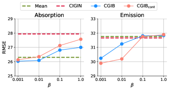
C.4 Quantitative Analysis on CIB-Graph

To verify the usefulness of the subgraphs (i.e., $\mathcal{G}_{\mathrm{CIB}}^{1}$) determined by CGIB and $\textsf{CGIB}_{\textrm{cont}}$, we train a baseline model, i.e., MPNN, with the importance scores (i.e., $p_{i}$) obtained from CGIB and $\textsf{CGIB}_{\textrm{cont}}$. Specifically, we replace the the graph readout function that is originally Set2Set (Vinyals et al., 2015) with the weighted sum pooling whose weights are based on the importance scores. Similarly, we train another baseline model based on the attention scores obtained from the interaction map of CIGIN (Pathak et al., 2020). Note that “Mean” indicates a baseline whose pooling function is Mean pooling, i.e., utilizing all the nodes equally. We have the following observations in Figure 6. 1) Attending to the subgraph determined by CGIB and $\textsf{CGIB}_{\textrm{cont}}$ outperforms the baseline model with Mean pooling function, indicating that our proposed models capture subgraphs that are useful for the task. Moreover, by comparing with the baseline model trained with subgraphs determined by CIGIN, we find out that CGIB and $\textsf{CGIB}_{\textrm{cont}}$ capture more useful subgraphs than CIGIN. 2) However, attending to the selected subgraphs does not always lead to performance improvements, i.e., when $\beta=0.1$ and $\beta=1.0$. This is because aggressive compression (i.e., large $\beta$) impedes the detection of the task-relevant subgraph, which eventually degrades the model performance. This aligns with our observation in Section 5.3.1. 3) Accordingly, the performance improves as $\beta$ decreases, because CGIB is trained to focus more on discovering the task-relevant part of the graph than aggressively compressing the graph.

Figure 6: Quantitative analysis on CIB-Graph.

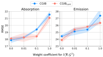
C.5 Sensitivity analysis on $I(\mathbf{Y};\mathcal{G}^{2})$

Recall that the prediction term of CGIB is decomposed as shown in Equation 9: $-I(\mathbf{Y};\mathcal{G}_{\mathrm{CIB}}^{1}|\mathcal{G}^{2})=-I(\mathbf{Y};\mathcal{G}_{\mathrm{CIB}}^{1},\mathcal{G}^{2})+I(\mathbf{Y};\mathcal{G}^{2})$, and our goal is to minimize this term. In this section, we analyze the effect of minimizing $I(\mathbf{Y};\mathcal{G}^{2})$ by conducting experiments on various weight coefficients for the term. Specifically, we minimize the upper bound of $I(\mathbf{Y};\mathcal{G}^{2})$, which is given as the Kullback-Leibler divergence between $p(\mathbf{Y}|\mathcal{G}^{2})$ and its variational approximation $r(\mathbf{Y})$ (Alemi et al., 2016). Following VIB (Alemi et al., 2016), we treat $r(\mathbf{Y})$ as a fixed spherical Gaussian, i.e., $r(\mathbf{Y})=\mathcal{N}(\mathbf{Y}|0,1)$. As shown in Figure 7, we find out that including $I(\mathbf{Y};\mathcal{G}^{2})$ into our objectives severely deteriorates the model performance. In other words, the model performs worse as the weight coefficient of $I(\mathbf{Y};\mathcal{G}^{2})$ gets larger, and the performance is the best when the weight coefficient is 0, i.e., when the term is not included in the optimization. This is because minimizing the conditional mutual information $-I(\mathbf{Y};\mathcal{G}_{\mathrm{CIB}}^{1}|\mathcal{G}^{2})$ is equivalent to predicting the target value $\mathbf{Y}$ given $\mathcal{G}_{\mathrm{CIB}}^{1}$ conditioned on $\mathcal{G}^{2}$, i.e., the model focuses more on $\mathcal{G}_{\mathrm{CIB}}^{1}$ and do not fully use the information of $\mathcal{G}^{2}$. Thus, we argue that in relational learning, where both entities in the pair are relevant to the target value $\mathbf{Y}$, considering only the joint mutual information $-I(\mathbf{Y};\mathcal{G}_{\mathrm{CIB}}^{1},\mathcal{G}^{2})$ is more beneficial than additionally considering the conditional mutual information for prediction.

Figure 7: Sensitivity Analysis on $I(\mathbf{Y};\mathcal{G}^{2})$.

C.6 Various modeling choices for $p_{\xi}$

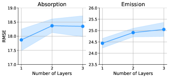
In Figure 8, we show experimental results adopting more complex modeling choices for $p_{\xi}$ used in Equation 13. We find out that as the number of layers increases, the model performs worse, demonstrating that a complex modeling of $p_{\xi}$ incurs the information loss during the prediction of $\mathcal{G}^{2}$.

Figure 8: Sensitivity analysis on the number of layers for $p_{\xi}$.

C.7 Qualitative analysis for $\beta$

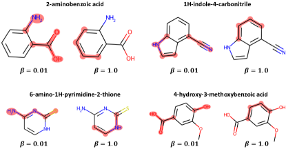
In Figure 9, we show how the model captures the core substructure according to $\beta$, which controls the trade-off between prediction and compression in our final objectives in Equation 15. We observe that the model better captures task relevant substructures when $\beta=0.01$ compared with the case when $\beta=1.0$. When $\beta=1.0$, the model concentrates on the aromatic ring, which is the structure that makes the molecules stable rather than directly related to chemical reactions. On the other hand, the model tends to discover the substructures related to chemical reactions when $\beta=0.01$. To sum up, as $\beta$ decreases, we find out that our model discovers more task-relevant but less compressed (i.e., large in scale) substructure of the molecule.

Figure 9: Qualitative analysis for $\beta$.

Appendix D Evaluation Protocol

For the molecular interaction prediction task, we evaluate the models under 5-fold cross validation scheme following the previous work (Pathak et al., 2020). The dataset is randomly split into 5 subsets and one of the subsets is used as the test set while the remaining subsets are used to train the model. A subset of the test set is selected as validation set for hyperparameter selection and early stopping. We repeat 5-fold cross validation 5 times (i.e., 25 runs in total) and report the accuracy and standard deviation of the repeats. For the DDI prediction task, we conduct experiments on both transductive and inductive settings. In the transductive setting, the graphs in test phase are also included in the training dataset. That is, we use a random split of the data into train/validation/test data of 60/20/20%, respectively, following SSI-DDI (Nyamabo et al., 2021). On the other hand, in the inductive setting, the performance is evaluated when the models are presented with new graphs that were not included in the training dataset. Specifically, let $\mathbb{G}$ denote the total set of graphs in the dataset. Given $\mathbb{G}$, we split $\mathbb{G}$ into $\mathbb{G}_{\mathrm{old}}$ and $\mathbb{G}_{\mathrm{new}}$, so that $\mathbb{G}_{\mathrm{old}}$ contains the set of graphs that have been seen in the training phase, and $\mathbb{G}_{\mathrm{new}}$ contains the set of graphs that have not been seen in the training phase. Then, the new split of dataset consists of $\mathcal{D}_{\mathrm{train}}=\{(\mathcal{G}^{1},\mathcal{G}^{2})\in\mathcal{D}|\mathcal{G}^{1}\in\mathbb{G}_{\mathrm{old}}\wedge\mathcal{G}^{2}\in\mathbb{G}_{\mathrm{old}}\}$ and $\mathcal{D}_{\mathrm{test}}=\{(\mathcal{G}^{1},\mathcal{G}^{2})\in\mathcal{D}|(\mathcal{G}^{1}\in\mathbb{G}_{\mathrm{new}}\wedge\mathcal{G}^{2}\in\mathbb{G}_{\mathrm{new}})\vee(\mathcal{G}^{1}\in\mathbb{G}_{\mathrm{new}}\wedge\mathcal{G}^{2}\in\mathbb{G}_{\mathrm{old}})\vee(\mathcal{G}^{1}\in\mathbb{G}_{\mathrm{old}}\wedge\mathcal{G}^{2}\in\mathbb{G}_{\mathrm{new}})\}$. We use a subset of $\mathcal{D}_{\mathrm{test}}$ as validation set in inductive setting. For both the transductive and inductive DDI tasks, we repeat 5 independent experiments with different random seeds on a split data, and report the accuracy and the standard deviation of the repeats. For the similarity learning task, we repeat 5 independent experiments with different random seeds on the already-split data given by (Zhang et al., 2021). For all tasks, we report the test performance when the performance on the validation set gives the best result.

Appendix E Implementation Details

Model architecture. For the molecular interaction prediction, we use two 3-layer MPNNs (Gilmer et al., 2017) as our backbone molecule encoder to learn the representation of solute and solvent, respectively. This is because the solute and solvent have different roles during the chemical reaction, thereby using a shared encoder may hard to capture the patterns in each solute and solvent. On the other hand, we use a GIN (Xu et al., 2018) to encode both drugs for the drug-drug interaction prediction task, and a GCN (Kipf & Welling, 2016) to encode both graphs for graph similarity learning. Different from molecular interaction prediction, those tasks have no specific roles between two entities. Therefore, we choose to share a encoder during the experiments.

Model Training. In all our experiments, we use the Adam optimizer for model optimization. For molecular interaction task and drug-drug interaction task, the learning rate was decreased on plateau by a factor of $10^{-1}$ with the patience of 20 epochs following previous work (Pathak et al., 2020). For similarity learning task, we do not use a learning rate scheduler for the fair comparison with $\text{H}^{2}\text{MN}$ (Zhang et al., 2021).

Hyperparameter Tuning. For fair comparisons, we follow the embedding dimensions and batch sizes of the state-of-the-art baseline for each task. Detailed hyperparameter specifications are given in Table 7. For the hyperparameters of CGIB, we tune them in certain ranges as follows: learning rate $\eta$ in $\{5e^{-3},1e^{-3},5e^{-4},1e^{-4},5e^{-5}\}$ and $\beta$ in $\{1e^{-1},1e^{-2},1e^{-3},1e^{-4},1e^{-6},1e^{-8},1e^{-10}\}$. We also tune the temperature $\tau$ in $\{1.0,0.5,0.2\}$ for $\textsf{CGIB}_{\textrm{cont}}$.

Table 7: Hyperparameter specifications ($*$: inductive task).

	Embedding	Batch	Epochs	CGIB		$\textsf{CGIB}_{\textrm{cont}}$
	Dim ($d$)	Size ($K$)		lr	$\beta$	lr	$\beta$	$\tau$
Absorption	52	256	500	5e-3	1e-3	5e-3	1e-1	1.0
Emission	52	256	500	5e-3	1e-1	5e-3	1e-2	1.0
Lifetime	52	256	500	5e-3	1e-6	1e-3	1e-6	1.0
MNSol	42	32	200	1e-3	1e-4	1e-3	1e-6	1.0
FreeSolv	42	32	200	1e-3	1e-10	5e-3	1e-8	1.0
CompSol	42	256	500	1e-3	1e-8	1e-3	1e-6	1.0
Abraham	42	256	500	1e-3	1e-6	1e-3	1e-10	1.0
CombiSolv	42	256	500	1e-3	1e-4	5e-3	1e-6	0.5
ZhangDDI	300	512	500	5e-4	1e-3	5e-4	1e-3	0.5
ChChMiner	300	512	500	5e-4	1e-4	5e-4	1e-3	0.2
$\text{ZhangDDI}^{*}$	300	512	500	5e-5	1e-4	5e-4	1e-4	1.0
$\text{ChChMiner}^{*}$	300	512	500	5e-4	1e-4	5e-4	1e-4	1.0
AIDS	100	512	10000	1e-4	1e-3	1e-4	1e-4	1.0
IMDB	100	256	10000	1e-4	1e-3	1e-4	1e-3	1.0
OpenSSL	100	16	10000	1e-4	1e-6	1e-4	1e-4	1.0

Training Resources. We conduct all the experiments using a 24GB NVIDIA GeForce RTX 3090.

References

- Alemi et al. (2016) Alemi, A. A., Fischer, I., Dillon, J. V., and Murphy, K. Deep variational information bottleneck. arXiv preprint arXiv:1612.00410, 2016.
- Alsentzer et al. (2020) Alsentzer, E., Finlayson, S., Li, M., and Zitnik, M. Subgraph neural networks. Advances in Neural Information Processing Systems, 33:8017–8029, 2020.
- Bai et al. (2019) Bai, Y., Ding, H., Bian, S., Chen, T., Sun, Y., and Wang, W. Simgnn: A neural network approach to fast graph similarity computation. In Proceedings of the Twelfth ACM International Conference on Web Search and Data Mining, pp. 384–392, 2019.
- Bai et al. (2020) Bai, Y., Ding, H., Gu, K., Sun, Y., and Wang, W. Learning-based efficient graph similarity computation via multi-scale convolutional set matching. In Proceedings of the AAAI Conference on Artificial Intelligence, volume 34, pp. 3219–3226, 2020.
- Book (2014) Book, G. Compendium of chemical terminology. International Union of Pure and Applied Chemistry, 528, 2014.
- Bunke (1997) Bunke, H. On a relation between graph edit distance and maximum common subgraph. Pattern recognition letters, 18(8):689–694, 1997.
- Bunke & Shearer (1998) Bunke, H. and Shearer, K. A graph distance metric based on the maximal common subgraph. Pattern recognition letters, 19(3-4):255–259, 1998.
- Deac et al. (2019) Deac, A., Huang, Y.-H., Veličković, P., Liò, P., and Tang, J. Drug-drug adverse effect prediction with graph co-attention. arXiv preprint arXiv:1905.00534, 2019.
- Delaney (2004) Delaney, J. S. Esol: estimating aqueous solubility directly from molecular structure. Journal of chemical information and computer sciences, 44(3):1000–1005, 2004.
- Feng et al. (2019) Feng, Y., You, H., Zhang, Z., Ji, R., and Gao, Y. Hypergraph neural networks. In Proceedings of the AAAI conference on artificial intelligence, volume 33, pp. 3558–3565, 2019.
- Gilmer et al. (2017) Gilmer, J., Schoenholz, S. S., Riley, P. F., Vinyals, O., and Dahl, G. E. Neural message passing for quantum chemistry. In International conference on machine learning, pp. 1263–1272. PMLR, 2017.
- Gontijo-Lopes et al. (2020) Gontijo-Lopes, R., Smullin, S., Cubuk, E. D., and Dyer, E. Tradeoffs in data augmentation: An empirical study. In International Conference on Learning Representations, 2020.
- Grubbs et al. (2010) Grubbs, L. M., Saifullah, M., Nohelli, E., Ye, S., Achi, S. S., Acree Jr, W. E., and Abraham, M. H. Mathematical correlations for describing solute transfer into functionalized alkane solvents containing hydroxyl, ether, ester or ketone solvents. Fluid phase equilibria, 298(1):48–53, 2010.
- Hjelm et al. (2018) Hjelm, R. D., Fedorov, A., Lavoie-Marchildon, S., Grewal, K., Bachman, P., Trischler, A., and Bengio, Y. Learning deep representations by mutual information estimation and maximization. arXiv preprint arXiv:1808.06670, 2018.
- Hynes (1985) Hynes, J. T. Chemical reaction dynamics in solution. Annual Review of Physical Chemistry, 36(1):573–597, 1985.
- Jang et al. (2016) Jang, E., Gu, S., and Poole, B. Categorical reparameterization with gumbel-softmax. arXiv preprint arXiv:1611.01144, 2016.
- Jerry (1992) Jerry, M. Advanced organic chemistry: reactions, mechanisms and structure, 1992.
- Joung et al. (2020) Joung, J. F., Han, M., Jeong, M., and Park, S. Experimental database of optical properties of organic compounds. Scientific data, 7(1):1–6, 2020.
- Joung et al. (2021) Joung, J. F., Han, M., Hwang, J., Jeong, M., Choi, D. H., and Park, S. Deep learning optical spectroscopy based on experimental database: Potential applications to molecular design. JACS Au, 1(4):427–438, 2021.
- Kastrin et al. (2018) Kastrin, A., Ferk, P., and Leskošek, B. Predicting potential drug-drug interactions on topological and semantic similarity features using statistical learning. PloS one, 13(5):e0196865, 2018.
- Kipf & Welling (2016) Kipf, T. N. and Welling, M. Semi-supervised classification with graph convolutional networks. arXiv preprint arXiv:1609.02907, 2016.
- Li et al. (2019) Li, Y., Gu, C., Dullien, T., Vinyals, O., and Kohli, P. Graph matching networks for learning the similarity of graph structured objects. In International conference on machine learning, pp. 3835–3845. PMLR, 2019.
- Lim & Jung (2019) Lim, H. and Jung, Y. Delfos: deep learning model for prediction of solvation free energies in generic organic solvents. Chemical science, 10(36):8306–8315, 2019.
- Ling et al. (2019) Ling, X., Wu, L., Wang, S., Ma, T., Xu, F., Wu, C., and Ji, S. Hierarchical graph matching networks for deep graph similarity learning. 2019.
- Maddison et al. (2016) Maddison, C. J., Mnih, A., and Teh, Y. W. The concrete distribution: A continuous relaxation of discrete random variables. arXiv preprint arXiv:1611.00712, 2016.
- Marenich et al. (2020) Marenich, A. V., Kelly, C. P., Thompson, J. D., Hawkins, G. D., Chambers, C. C., Giesen, D. J., Winget, P., Cramer, C. J., and Truhlar, D. G. Minnesota solvation database (mnsol) version 2012. 2020.
- Meng et al. (2018) Meng, C., Mouli, S. C., Ribeiro, B., and Neville, J. Subgraph pattern neural networks for high-order graph evolution prediction. In Proceedings of the AAAI Conference on Artificial Intelligence, volume 32, 2018.
- Miao et al. (2022) Miao, S., Liu, M., and Li, P. Interpretable and generalizable graph learning via stochastic attention mechanism. In International Conference on Machine Learning, pp. 15524–15543. PMLR, 2022.
- Mobley & Guthrie (2014) Mobley, D. L. and Guthrie, J. P. Freesolv: a database of experimental and calculated hydration free energies, with input files. Journal of computer-aided molecular design, 28(7):711–720, 2014.
- Moine et al. (2017) Moine, E., Privat, R., Sirjean, B., and Jaubert, J.-N. Estimation of solvation quantities from experimental thermodynamic data: Development of the comprehensive compsol databank for pure and mixed solutes. Journal of Physical and Chemical Reference Data, 46(3):033102, 2017.
- Nyamabo et al. (2021) Nyamabo, A. K., Yu, H., and Shi, J.-Y. Ssi–ddi: substructure–substructure interactions for drug–drug interaction prediction. Briefings in Bioinformatics, 22(6):bbab133, 2021.
- Pan et al. (2021) Pan, Z., Niu, L., Zhang, J., and Zhang, L. Disentangled information bottleneck. In Proceedings of the AAAI Conference on Artificial Intelligence, volume 35, pp. 9285–9293, 2021.
- Pathak et al. (2020) Pathak, Y., Laghuvarapu, S., Mehta, S., and Priyakumar, U. D. Chemically interpretable graph interaction network for prediction of pharmacokinetic properties of drug-like molecules. In Proceedings of the AAAI Conference on Artificial Intelligence, volume 34, pp. 873–880, 2020.
- Preuer et al. (2018) Preuer, K., Lewis, R. P., Hochreiter, S., Bender, A., Bulusu, K. C., and Klambauer, G. Deepsynergy: predicting anti-cancer drug synergy with deep learning. Bioinformatics, 34(9):1538–1546, 2018.
- Purser et al. (2008) Purser, S., Moore, P. R., Swallow, S., and Gouverneur, V. Fluorine in medicinal chemistry. Chemical Society Reviews, 37(2):320–330, 2008.
- Reichardt (1965) Reichardt, C. Empirical parameters of the polarity of solvents. Angewandte Chemie International Edition in English, 4(1):29–40, 1965.
- Rozemberczki et al. (2021) Rozemberczki, B., Bonner, S., Nikolov, A., Ughetto, M., Nilsson, S., and Papa, E. A unified view of relational deep learning for drug pair scoring. arXiv preprint arXiv:2111.02916, 2021.
- Singh et al. (2009) Singh, T. S., Moyon, N., and Mitra, S. Effect of solvent hydrogen bonding on the photophysical properties of intramolecular charge transfer probe trans-ethyl p-(dimethylamino) cinamate and its derivative. Spectrochimica Acta Part A: Molecular and Biomolecular Spectroscopy, 73(4):630–636, 2009.
- Sun et al. (2022) Sun, Q., Li, J., Peng, H., Wu, J., Fu, X., Ji, C., and Philip, S. Y. Graph structure learning with variational information bottleneck. In Proceedings of the AAAI Conference on Artificial Intelligence, volume 36, pp. 4165–4174, 2022.
- Tian et al. (2020) Tian, Y., Krishnan, D., and Isola, P. Contrastive multiview coding. In European conference on computer vision, pp. 776–794. Springer, 2020.
- Tishby et al. (2000) Tishby, N., Pereira, F. C., and Bialek, W. The information bottleneck method. arXiv preprint physics/0004057, 2000.
- Veličković et al. (2017) Veličković, P., Cucurull, G., Casanova, A., Romero, A., Lio, P., and Bengio, Y. Graph attention networks. 2017.
- Veličković et al. (2018) Veličković, P., Fedus, W., Hamilton, W. L., Liò, P., Bengio, Y., and Hjelm, R. D. Deep graph infomax. arXiv preprint arXiv:1809.10341, 2018.
- Vermeire & Green (2021) Vermeire, F. H. and Green, W. H. Transfer learning for solvation free energies: From quantum chemistry to experiments. Chemical Engineering Journal, 418:129307, 2021.
- Vilar et al. (2012) Vilar, S., Harpaz, R., Uriarte, E., Santana, L., Rabadan, R., and Friedman, C. Drug—drug interaction through molecular structure similarity analysis. Journal of the American Medical Informatics Association, 19(6):1066–1074, 2012.
- Vinyals et al. (2015) Vinyals, O., Bengio, S., and Kudlur, M. Order matters: Sequence to sequence for sets. arXiv preprint arXiv:1511.06391, 2015.
- Wang et al. (2021) Wang, Y., Min, Y., Chen, X., and Wu, J. Multi-view graph contrastive representation learning for drug-drug interaction prediction. In Proceedings of the Web Conference 2021, pp. 2921–2933, 2021.
- Wu et al. (2020) Wu, T., Ren, H., Li, P., and Leskovec, J. Graph information bottleneck. Advances in Neural Information Processing Systems, 33:20437–20448, 2020.
- Xu et al. (2018) Xu, K., Hu, W., Leskovec, J., and Jegelka, S. How powerful are graph neural networks? arXiv preprint arXiv:1810.00826, 2018.
- Xu et al. (2017) Xu, X., Liu, C., Feng, Q., Yin, H., Song, L., and Song, D. Neural network-based graph embedding for cross-platform binary code similarity detection. In Proceedings of the 2017 ACM SIGSAC Conference on Computer and Communications Security, pp. 363–376, 2017.
- You et al. (2020) You, Y., Chen, T., Sui, Y., Chen, T., Wang, Z., and Shen, Y. Graph contrastive learning with augmentations. Advances in Neural Information Processing Systems, 33:5812–5823, 2020.
- Yu et al. (2020) Yu, J., Xu, T., Rong, Y., Bian, Y., Huang, J., and He, R. Graph information bottleneck for subgraph recognition. arXiv preprint arXiv:2010.05563, 2020.
- Yu et al. (2022) Yu, J., Cao, J., and He, R. Improving subgraph recognition with variational graph information bottleneck. In Proceedings of the IEEE/CVF Conference on Computer Vision and Pattern Recognition, pp. 19396–19405, 2022.
- Zhang et al. (2017) Zhang, W., Chen, Y., Liu, F., Luo, F., Tian, G., and Li, X. Predicting potential drug-drug interactions by integrating chemical, biological, phenotypic and network data. BMC bioinformatics, 18(1):1–12, 2017.
- Zhang et al. (2021) Zhang, Z., Bu, J., Ester, M., Li, Z., Yao, C., Yu, Z., and Wang, C. H2mn: Graph similarity learning with hierarchical hypergraph matching networks. In Proceedings of the 27th ACM SIGKDD Conference on Knowledge Discovery & Data Mining, pp. 2274–2284, 2021.
- Zhou et al. (2006) Zhou, D., Huang, J., and Schölkopf, B. Learning with hypergraphs: Clustering, classification, and embedding. Advances in neural information processing systems, 19, 2006.
- Zhu et al. (2021) Zhu, Y., Xu, Y., Yu, F., Liu, Q., Wu, S., and Wang, L. Graph contrastive learning with adaptive augmentation. In Proceedings of the Web Conference 2021, pp. 2069–2080, 2021.
- Zitnik et al. (2018) Zitnik, M., Sosic, R., and Leskovec, J. Biosnap datasets: Stanford biomedical network dataset collection. Note: http://snap. stanford. edu/biodata Cited by, 5(1), 2018.