A Parameter-free Adaptive Resonance Theory-based Topological Clustering Algorithm
Capable of Continual Learning

Abstract

In general, a similarity threshold (i.e., a vigilance parameter) for a node learning process in Adaptive Resonance Theory (ART)-based algorithms has a significant impact on clustering performance. In addition, an edge deletion threshold in a topological clustering algorithm plays an important role in adaptively generating well-separated clusters during a self-organizing process. In this paper, we propose a new parameter-free ART-based topological clustering algorithm capable of continual learning by introducing parameter estimation methods. Experimental results with synthetic and real-world datasets show that the proposed algorithm has superior clustering performance to the state-of-the-art clustering algorithms without any parameter pre-specifications.

1 Introduction

The recent growth of Internet of Things (IoT) technology has enabled the creation and acquisition of a wide variety of data. Such data are regarded as important economic resources that can be used for marketing, finance, and IoT solution development. Supervised learning and unsupervised learning are typical approaches for analyzing the acquired data and extracting useful information. In general, supervised learning algorithms require a sufficient amount of labeled training data for achieving high information extraction performance. In contrast, unsupervised learning such as clustering can extract useful information without requiring labeled training data. $k$-means [1], Gaussian Mixture Model (GMM) [2], and Self-Organizing Map (SOM) [3] are typical clustering algorithms. Although $k$-means, GMM, and SOM are quite simple and highly applicable, these algorithms have to specify the number of clusters or the size of the network in advance. This drawback makes it difficult to apply these algorithms to data whose distributions are unknown and/or continually changing.

Growing Neural Gas (GNG) [4] and Adjusted Self-Organizing Incremental Neural Network (ASOINN) [5] can adaptively generate topological networks (i.e., nodes and edges) depending on the distributions of given data. Thus, these algorithms do not require any pre-defined parameters unlike $k$-means and SOM. Thanks to this feature, these algorithms are used as an information extraction method in unknown environments, such as simultaneous localization and mapping [6], and knowledge acquisition for robots [7]. However, GNG and SOINN tend to permanently and excessively generate nodes in their networks for memorizing new information, which may collapse learned information. This trade-off is called the plasticity-stability dilemma [8].

Adaptive Resonance Theory (ART) [9, 10] is one of the most successful approaches for handling the plasticity-stability dilemma while realizing continual learning. ART-based topological clustering algorithms [11, 12], which use Correntropy-Induced Metric (CIM) [13] as a similarity measure, show faster and more stable self-organizing ability than other ART-based algorithms [9, 14, 15, 16]. However, these algorithms have two data-dependent parameters, namely a similarity threshold (i.e., a vigilance parameter) for a node learning process and an edge deletion threshold for a topology adjustment method, which have a significant impact on their clustering performance.

This paper proposes a new parameter-free ART-based topological clustering algorithm, called CIM-based ART with Edge (CAE), by introducing two parameter estimation methods to CIM-based ART with Edge and Age (CAEA) [12]. In the proposed algorithm, a similarity threshold is calculated based on pairwise similarities among a certain number of nodes. The sufficient number of nodes for calculating the similarity threshold is estimated by a Determinantal Point Processes (DPP)-based criterion [17, 18]. In addition, an edge deletion threshold is estimated based on the age of each edge, which is inspired by the edge deletion mechanism of SOINN+ [19]. Thanks to the parameter estimation methods, the proposed algorithm can adaptively, efficiently, and continually generate a topological network from the given data while maintaining superior clustering performance to conventional algorithms. Note that continual learning is generally categorized into three scenarios, namely domain incremental learning, task incremental learning, and class incremental learning [20, 21]. This paper focuses on class incremental learning problems.

The contributions of this paper are summarized as follows:

• CAE is proposed as a new parameter-free ART-based clustering algorithm capable of continual learning.

• An estimation method of the number of nodes for calculating a similarity threshold is introduced to CAE. The sufficient number of nodes for calculating the threshold is estimated by a DPP-based criterion incorporating CIM.

• An estimation method of a node deletion threshold is introduced to CAE, which is inspired by the edge deletion method of SOINN+ [19]. The node deletion threshold is estimated based on the age of each edge.

• Empirical studies show that CAE has superior clustering performance to the state-of-the-art algorithms without any parameter specifications while maintaining continual learning ability.

The paper is organized as follows. Section 2 presents a literature review for growing self-organizing clustering and clustering-based classification algorithms capable of continual learning. Section 3 presents the preliminary knowledge for a similarity measure and a kernel density estimator used in CAE. Section 4 presents the learning procedure of CAE in detail. Section 5 presents extensive simulation experiments to evaluate clustering performance by using synthetic and real-world datasets. Section 6 concludes this paper.

2 Literature Review

2.1 Growing Self-organizing Clustering Algorithms

Classical clustering algorithms such as Gaussian Mixture Model (GMM) [2] and $k$-means [1] have shown their adaptability and applicability in many fields. However, the major drawback of these algorithms is that the number of clusters/partitions has to be pre-specified. To solve this problem, growing self-organizing clustering algorithms such as GNG [4] and ASOINN [5] have been proposed. GNG and ASOINN adaptively generate topological networks (i.e., nodes and edges) for representing the distributions of given data. However, since these algorithms permanently insert new nodes and edges for learning new information, there is a possibility to forget previously learned information (i.e., catastrophic forgetting). More generally, this phenomenon is called the plasticity-stability dilemma [8]. As a GNG-based algorithm, Grow When Required (GWR) [22] can avoid the plasticity-stability dilemma by adding nodes whenever the state of the current network does not sufficiently match the instance. SOINN+ [19] is an ASOINN-based algorithm that can detect clusters of arbitrary shapes in noisy data streams without any pre-defined parameters. One common problem of GWR and SOINN+ is that as the number of nodes in the network increases, the cost of calculating a threshold for each node increases, and thus the learning efficiency decreases.

One promising approach for avoiding the plasticity-stability dilemma is an ART-based algorithm that uses a pre-defined similarity threshold (i.e., a vigilance parameter) for controlling a learning process. Thanks to this property, many ART-based clustering algorithms and their improvements have been proposed [9, 14, 15, 23]. In particular, algorithms that use CIM as a similarity measure have shown superior clustering performance to other clustering algorithms [24, 25, 11, 26]. A well-known drawback of ART-based algorithms is the specification of significantly data-dependent parameters such as a similarity threshold (i.e., a vigilance parameter). Several studies have proposed to avoid and/or suppress the effect of the above-mentioned drawback by applying multiple vigilance values [27], by specifying the vigilance parameter indirectly [28, 12], and by adjusting some data-dependent parameters during the learning process [29]. However, parameters to be pre-specified still exist in these algorithms, which affect their clustering performance.

2.2 Clustering-based Classification Algorithms Capable of Continual Learning

Recently, deep learning has shown outstanding capability in many fields, such as image processing and natural language processing [30, 31, 32]. In contrast, the continual learning ability of deep learning is not sufficient [33]. Continual learning is categorized into three scenarios [20, 21]: domain incremental learning [34, 35], task incremental learning [36], and class incremental learning [37, 36, 38, 39]. In general, deep learning capable of continual learning uses selective learning of weight coefficients between neurons or sequential addition of neurons in the output layer corresponding to new information. However, the major problem with this approach is that a network structure for representation learning is basically fixed, and therefore, there is an upper limit to the memory capacity of the entire network.

In general, a clustering algorithm can be applied to classification tasks by using a clustering result (e.g., cluster centroids, topological networks) as a classifier [40, 41, 42, 16]. Note that, in many cases, a clustering-based classification algorithm can inherit the continual learning ability from a clustering algorithm [43, 14, 24]. This fact enhances the attractiveness of clustering capable of continual learning and motivates us to develop clustering-based classification algorithms. Typical clustering-based classification algorithms are Episodic-GWR (EGWR) [7] and ASOINN Classifier (ASC) [5], which use GWR and ASOINN, respectively, for generating base classifiers. AutoCloud [44] is a fully online algorithm that autonomously creates clusters and merges them. AutoCloud is a quite flexible algorithm that can be used for unsupervised, semi-supervised, and supervised classification tasks. The state-of-the-art clustering-based classification algorithm is GSOINN+ [45]. GSOINN+ is an extended algorithm of SOINN+, which uses ghost nodes and a weighted nearest-neighbor rule based on the fractional distance for classification tasks. Although GSOINN+ successfully adapts to supervised learning, there are two parameters to be pre-specified for maintaining good classification performance. ART-based classification algorithms (e.g., ARTMAP) are also successful approaches [43, 14, 24, 46, 47, 48]. However, similar to ART-based clustering algorithms, ART-based classification algorithms also suffer from the difficulty of the specification of parameters for maintaining good classification performance. A small number of studies have focused on specification/adjustment methods for significantly data-dependent parameters [48, 16, 49, 50, 51]. However, these studies still have parameters that need to be adjusted for each dataset. This fact emphasizes the significance of developing parameter-free clustering algorithms capable of continual learning.

3 Preliminary Knowledge

This section presents preliminary knowledge for a similarity measure and a kernel density estimator used in the proposed CAE algorithm.

3.1 Correntropy and Correntropy-induced Metric

Correntropy [13] provides a generalized similarity measure between two arbitrary data points $\mathbf{x}=(x_{1},x_{2},\ldots,x_{d})$ and $\mathbf{y}=(y_{1},y_{2},\ldots,y_{d})$ as follows:

$$C(\mathbf{x},\mathbf{y})=\textbf{E}\left[\kappa_{\sigma}\left(\mathbf{x},\mathbf{y}\right)\right],$$ (1)

where $\textbf{E}\left[\cdot\right]$ is the expectation operation, and $\kappa_{\sigma}\left(\cdot\right)$ denotes a positive definite kernel with a bandwidth $\sigma$. The correntropy can be estimated as follows:

$$\hat{C}(\mathbf{x},\mathbf{y})=\frac{1}{d}\sum_{i=1}^{d}\kappa_{\sigma}\left(x_{i},y_{i}\right).$$ (2)

In this paper, we use the following Gaussian kernel in the correntropy:

$$\kappa_{\sigma}\left(x_{i},y_{i}\right)=\exp\left[-\frac{\left(x_{i}-y_{i}\right)^{2}}{2\sigma^{2}}\right].$$ (3)

A nonlinear metric called CIM is derived from the correntropy [13]. CIM quantifies the similarity between two data points $\mathbf{x}$ and $\mathbf{y}$ as follows:

$$\mathrm{CIM}\left(\mathbf{x},\mathbf{y},\sigma\right)=\left[1-\hat{C}(\mathbf{x},\mathbf{y})\right]^{\frac{1}{2}}.$$ (4)

Here, thanks to the Gaussian kernel without a coefficient $\frac{1}{\sqrt{2\pi}\sigma}$ as defined in (3), a range of CIM is limited to $\left[0,1\right]$.

In general, the Euclidean distance suffers from the curse of dimensionality. However, CIM reduces this drawback thanks to the correntropy which calculates the similarity between two arbitrary data points by using a kernel function. Moreover, it has also been shown that CIM with the Gaussian kernel has a high outlier rejection capability [13].

3.2 Kernel Density Estimator

In general, the bandwidth of a kernel function can be estimated from $\lambda$ instances belonging to a certain distribution [52], which is defined as follows:

$$\bm{\Sigma}=U(F_{\nu})\bm{\Gamma}\lambda^{-\frac{1}{2\nu+d}},$$ (5)

$$U(F_{\nu})=\left(\frac{\pi^{d/2}2^{d+\nu-1}(\nu!)^{2}R(F)^{d}}{\nu\kappa_{\nu}^{2}(F)\left[(2\nu)!!+(d-1)(\nu!!)^{2}\right]}\right)^{\frac{1}{2\nu+d}},$$ (6)

where $\bm{\Gamma}$ denotes a rescale operator ($d$-dimensional vector) which is defined by a standard deviation of the $d$ attributes among $\lambda$ instances, $\nu$ is the order of a kernel, $R(F)$ is a roughness function, and $\kappa_{\nu}(F)$ is the moment of a kernel. The details of the derivation of (5) and (6) can be found in [52]. In this paper, we use the Gaussian kernel for CIM. Therefore, $\nu=2$, $R(F)=(2\sqrt{\pi})^{-1}$, and $\kappa_{\nu}^{2}(F)=1$ are derived, and (6) is rewritten as follows:

$$\mathbf{H}=\left(\frac{4}{2+d}\right)^{\frac{1}{4+d}}\bm{\Gamma}\lambda^{-\frac{1}{4+d}},$$ (7)

Equation (7) is known as the Silverman’s rule [53]. Here, $\mathbf{H}$ contains the bandwidth of each attribute.

4 Proposed Algorithm

4.1 Overview

The proposed CAE algorithm is an extended algorithm of CAEA [12] which is the state-of-the-art ART-based topological clustering algorithm. CAEA has two data-dependent parameters to be pre-specified, i.e., the number of nodes $\lambda$ for calculating a similarity threshold, and a threshold $a_{\text{max}}$ for an edge deletion process. Different from CAEA, CAE estimates these parameters during a learning process, i.e., the sufficient number of nodes $\lambda$ for calculating a similarity threshold is estimated by a DPP-based criterion incorporating CIM, and the node deletion threshold $a_{\text{max}}$ is estimated based on the age of each edge.

Table I summarizes the main notations used in this paper. The following subsections provide the learning processes of CAE step by step. Algorithm 1 summarizes the entire learning procedure of CAE.

TABLE I: Summary of notations

Notation	Description
$\mathbf{x}$	$d$-dimensional data point
$\mathcal{X}$	set of data points ($\mathbf{x}\in\mathcal{X}$)
$\mathbf{y}_{k}$	$k$-th node
$\mathcal{Y}$	set of nodes ($\mathbf{y}_{k}\in\mathcal{Y}$)
$|\mathcal{Y}|$	number of nodes in $\mathcal{Y}$
$\mathbf{y}_{s_{1}}$	1st winner node
$\mathbf{y}_{s_{2}}$	2nd winner node
$\sigma$	bandwidth of a kernel function
$\mathcal{S}$	set of bandwidths of a kernel function
$\mathcal{N}_{k}$	set of neighbor nodes of node $\mathbf{y}_{k}$
$\lambda$	number of active nodes
$\mathcal{A}$	set of active nodes
$D$	diversity of active nodes
$V_{s_{1}}$	CIM value between a data point $\mathbf{x}$ and $\mathbf{y}_{s_{1}}$
$V_{s_{2}}$	CIM value between a data point $\mathbf{x}$ and $\mathbf{y}_{s_{2}}$
$\mathbf{R}$	matrix of pairwise similarities
$V_{\text{threshold}}$	similarity threshold (a vigilance parameter)
$M_{k}$	number of winning counts of $\mathbf{y}_{k}$
$\mathcal{M}$	set of winning counts $M_{k}$ ($M_{k}\in\mathcal{M}$)
$a(\mathbf{y}_{k},\mathbf{y}_{l})$	age of an edge between nodes $\mathbf{y}_{k}$ and $\mathbf{y}_{l}\in\mathcal{Y}\setminus\mathbf{y}_{k}$
$\mathcal{E}$	set of ages of edges ($a(\mathbf{y}_{k},\mathbf{y}_{l})\in\mathcal{E}$)
$\alpha_{\text{del}}$	set of ages of deleted edges
$a_{\text{max}}$	edge deletion threshold

Input:

a set of data points $\mathcal{X}$.

Output:

a set of nodes $\mathcal{Y}$,

a set of ages of edges $\mathcal{E}$.

1 while  existing data points to be trained  do

2       Input a data point $\mathbf{x}$ ($\mathbf{x}\in\mathcal{X}$).

3      

4      if the number of active nodes $\lambda$ is not defined or the number of nodes $|\mathcal{Y}|$ is smaller than $\lambda/2$ or a similarity threshold $V_{\text{threshold}}$ is not calculated then

5             Create a node as $\mathbf{y}_{|\mathcal{Y}|+1}=\mathbf{x}$, and update a set of nodes as $\mathcal{Y}\leftarrow\mathcal{Y}\cup\{\mathbf{y}_{|\mathcal{Y}|+1}\}$.

             Estimate the diversity of nodes.

              // Algorithm 2

6             if the diversity of nodes is sufficient (i.e., $D<1.0\mathrm{e}{-6}$) then

7                   Calculate a similarity threshold $V_{\text{threshold}}$.

8                  

9            

10       else

11             Select the 1st and 2nd nearest nodes from $\mathbf{x}$ (i.e., $\mathbf{y}_{s_{1}}$ and $\mathbf{y}_{s_{2}}$) based on CIM.

             Perform vigilance test, and create/update nodes and edges.

              // Algorithm 3

             Estimate an edge deletion threshold $a_{\text{max}}$.

              // Algorithm 4

             Delete edges by using $a_{\text{max}}$.

              // Algorithm 5

12            

13      if the number of presented data points is a multiple of $\lambda$ then

14             Delete isolated nodes.

15      

Algorithm 1 Learning procedure of CAE

4.2 Estimation of Diversity of Nodes

In CAE, a similarity threshold is defined by a pairwise similarity among nodes (i.e., $\mathcal{Y}$) (see Section 4.3 for details). Thus, the diversity of nodes for calculating the similarity threshold is important to obtain an appropriate threshold value, which leads to good clustering performance.

The diversity $D$ of the node set $\mathcal{Y}$ is estimated by a DPP-based criterion [17, 18] incorporating CIM as follows:

$$D=\det(\mathbf{R}),$$ (8)

where

$$\mathbf{R}=\left[\exp\left(1-\mathrm{CIM}(\mathbf{y}_{i},\mathbf{y}_{j},\sigma)\right)\right]_{1\leq i,j\leq|\mathcal{Y}|}.$$ (9)

Here, $D$ is a determinant of the matrix $\mathbf{R}$, and $\mathbf{R}$ is a matrix of pairwise similarities between nodes in $\mathcal{Y}$. A bandwidth $\sigma$ for CIM is calculated from $\mathbf{H}$ in (7) by using a set of nodes $\mathcal{Y}$. As in (7), $\mathbf{H}$ contains a bandwidth of each attribute. In this paper, the median of $\mathbf{H}$ is used as the bandwidth of the Gaussian kernel in CIM, i.e.,

$$\sigma=\mathrm{median}\left(\mathbf{H}\right).$$ (10)

In general, the diversity $D=0$ means that the set of nodes $\mathcal{Y}$ is not diverse while $D>0$ means $\mathcal{Y}$ is diverse. In other words, the value of $D$ becomes close to zero when a new node is created around the existing nodes.

Input:

a data point $\mathbf{x}$,

a set of nodes $\mathcal{Y}$,

the number of active node $\lambda$.

Output:

diversity $D$,

the number of active nodes $\lambda$.

Calculate a pairwise similarity matrix $\mathbf{R}$.

  // (9)

Calculate the diversity as $D=\det(\mathbf{R})$.

  // (8)

1 if $D<1.0\mathrm{e}{-6}$ then

2       $\lambda=2|\mathcal{Y}|$

3 else

4       $\lambda=\infty$

Algorithm 2 Estimate diversity of nodes

Algorithm 2 summarizes the estimation process of the diversity of nodes. In CAE, the value of $\lambda$ is set as the two times of the number of nodes (i.e., $2|\mathcal{Y}|$) when the diversity $D$ satisfies $D<1.0\mathrm{e}{-6}$. If the number of nodes becomes smaller than $\lambda/2$ after a node deletion process, $\lambda$ is calculated again in line 5 of Algorithm 1 using Algorithm 2.

As shown in lines 3-4 of Algorithm 1, the first $\lambda/2$ data points (i.e., $\{\mathbf{x}_{1},\mathbf{x}_{2},\ldots\mathbf{x}_{\lambda/2}\}$) directly become nodes, i.e., $\mathcal{Y}=\{\mathbf{y}_{1},\mathbf{y}_{2},\ldots,\mathbf{y}_{\lambda/2}\}$ where $\mathbf{y}_{k}=\mathbf{x}_{k}$ $(k=1,2,\ldots,\lambda/2)$. In addition, the bandwidth for the Gaussian kernel in CIM is assigned to each node, i.e., $\mathcal{S}=\{\sigma_{1},\sigma_{2},\ldots,\sigma_{\lambda/2}\}$ where $\sigma_{1}=\sigma_{2}=\cdots=\sigma_{\lambda/2}$.

The value of $\lambda$ is automatically updated by Algorithm 2 in the proposed CAE algorithm. In an active node set $\mathcal{A}$, $\lambda$ nodes are stored. When a new node is added to $\mathcal{A}$, an old node is removed to maintain the active node set size as $\lambda$. The addition of a new node and the removal of an old node are explained later.

4.3 Calculation of Similarity Threshold

The similarity threshold $V_{\text{threshold}}$ is calculated by the average of the minimum pairwise CIM values in the active node set $\mathcal{A}$ as follows:

$$V_{\text{threshold}}=\frac{1}{\lambda}\sum_{\mathbf{y}_{i}\in\mathcal{A}}\min_{\mathbf{y}_{j}\in\mathcal{A}\setminus\mathbf{y}_{i}}\left[\mathrm{CIM}\left(\mathbf{y}_{i},\mathbf{y}_{j},\mathrm{mean}(\mathcal{S})\right)\right],$$ (11)

where $\mathcal{S}$ is a set of bandwidths of the Gaussian kernel in CIM for each node in $\mathcal{A}$, which are calculated by using (7) and (10) when a new node is created.

4.4 Selection of Winner Nodes

During the learning process of CAE, every time a data point $\mathbf{x}$ is given, two nodes which have a similar state to $\mathbf{x}$ are selected from $\mathcal{Y}$, namely the 1st winner node $\mathbf{y}_{s_{1}}$ and the 2nd winner node $\mathbf{y}_{s_{2}}$. The winner nodes are determined based on the value of CIM in line 9 of Algorithm 1 as follows:

$$s_{1}=\mathop{\rm\text{arg~{}min}}\limits_{\mathbf{y}_{i}\in\mathcal{Y}}\left[\mathrm{CIM}\left(\mathbf{x},\mathbf{y}_{i},\mathrm{mean}(\mathcal{S})\right)\right],$$ (12)

$$s_{2}=\mathop{\rm\text{arg~{}min}}\limits_{\mathbf{y}_{i}\in\mathcal{Y}\backslash\{\mathbf{y}_{s_{1}}\}}\left[\mathrm{CIM}\left(\mathbf{x},\mathbf{y}_{i},\mathrm{mean}(\mathcal{S})\right)\right],$$ (13)

where $s_{1}$ and $s_{2}$ denote the indexes of the 1st and 2nd winner nodes, respectively. $\mathcal{S}=\{\sigma_{1},\sigma_{2},\ldots,\sigma_{|\mathcal{Y}|}\}$ is a set of bandwidths of the Gaussian kernel in CIM corresponding to a set of nodes $\mathcal{Y}$.

Note that the 1st winner node $\mathbf{y}_{s_{1}}$ becomes a new active node, and the oldest node in the active node set $\mathcal{A}$ (i.e., $\lambda$ nodes in $\mathcal{Y}$) is replaced by the new one.

4.5 Vigilance Test

Similarities between the data point $\mathbf{x}$ and the 1st and 2nd winner nodes are defined in line 10 of Algorithm 1 as inputs for Algorithm 3.

as follows:

$$V_{s_{1}}=\mathrm{CIM}\left(\mathbf{x},\mathbf{y}_{s_{1}},\mathrm{mean}(\mathcal{S})\right),$$ (14)

$$V_{s_{2}}=\mathrm{CIM}\left(\mathbf{x},\mathbf{y}_{s_{2}},\mathrm{mean}(\mathcal{S})\right).$$ (15)

The vigilance test classifies the relationship between the data point $\mathbf{x}$ and the two winner nodes into three cases by using the similarity threshold $V_{\text{threshold}}$, i.e.,

• Case I
  The similarity between the data point $\mathbf{x}$ and the 1st winner node $\mathbf{y}_{s_{1}}$ is larger (i.e., less similar) than $V_{\text{threshold}}$, namely:

  $$V_{\text{threshold}}<V_{s_{1}}\leq V_{s_{2}}.$$ (16)

• Case II
  The similarity between the data point $\mathbf{x}$ and the 1st winner node $\mathbf{y}_{s_{1}}$ is smaller (i.e., more similar) than $V_{\text{threshold}}$, and the similarity between the data point $\mathbf{x}$ and the 2nd winner node $\mathbf{y}_{s_{2}}$ is larger (i.e., less similar) than $V_{\text{threshold}}$, namely:

  $$V_{s_{1}}\leq V_{\text{threshold}}<V_{s_{2}}.$$ (17)

• Case III
  The similarities between the data point $\mathbf{x}$ and the 1st and 2nd winner nodes are both smaller (i.e., more similar) than $V_{\text{threshold}}$, namely:

  $$V_{s_{1}}\leq V_{s_{2}}\leq V_{\text{threshold}}.$$ (18)

4.6 Creation/Update of Nodes and Edges

Depending on the result of the vigilance test, a different operation is performed.

If the data point $\mathbf{x}$ is classified as Case I by the vigilance test (i.e., (16) is satisfied), a new node is created as $\mathbf{y}_{|\mathcal{Y}|+1}=\mathbf{x}$, and updated a set of nodes as $\mathcal{Y}\leftarrow\mathcal{Y}\cup\{\mathbf{y}_{|\mathcal{Y}|+1}\}$. Here, the node $\mathbf{y}_{|\mathcal{Y}|+1}$ becomes a new active node, and the oldest node in the active node set $\mathcal{A}$ (i.e., $\lambda$ nodes in $\mathcal{Y}$) is replaced by the new one. In addition, a bandwidth $\sigma_{|\mathcal{Y}|+1}$ for $\mathbf{y}_{|\mathcal{Y}|+1}$ is calculated by (7) and (10) with the active node set $\mathcal{A}$, and the number of winning counts of $\mathbf{y}_{|\mathcal{Y}|+1}$ is initialized as $M_{|\mathcal{Y}|+1}=1$.

If the data point $\mathbf{x}$ is classified as Case II by the vigilance test (i.e., (17) is satisfied), first, the number of winning counts of $\mathbf{y}_{s_{1}}$ is updated as follows:

$$M_{s_{1}}\leftarrow M_{s_{1}}+1.$$ (19)

Then, $\mathbf{y}_{s_{1}}$ is updated as follows:

$$\mathbf{y}_{s_{1}}\leftarrow\mathbf{y}_{s_{1}}+\frac{1}{M_{s_{1}}}\left(\mathbf{x}-\mathbf{y}_{s_{1}}\right).$$ (20)

Here, the node $\mathbf{y}_{s_{1}}$ becomes a new active node, and the oldest node in the active node set $\mathcal{A}$ (i.e., $\lambda$ nodes in $\mathcal{Y}$) is replaced by the new one.

When updating the node, the difference between $\mathbf{x}$ and $\mathbf{y}$ is divided by $M_{s_{1}}$. Thus, the change of the node position is smaller when $M_{s_{1}}$ is larger. This is because the information around a node, where data points are frequently given, is important and should be held by the node.

The age of each edge connected to the first winner node $\mathbf{y}_{k_{1}}$ is also updated as follows:

$$a{(\mathbf{y}_{s_{1}},\mathbf{y}_{k})}\leftarrow a{(\mathbf{y}_{s_{1}},\mathbf{y}_{k})}+1\quad(\mathbf{y}_{k}\in\mathcal{N}_{s_{1}}),$$ (21)

where $\mathcal{N}_{s_{1}}$ is a set of all neighbor nodes of the node $\mathbf{y}_{s_{1}}$.

If the data point ${\mathbf{x}}$ is classified as Case III by the vigilance test (i.e., (18) is satisfied), the same operations as Case II (i.e., (19)-(21)) are performed. In addition, the neighbor nodes of $\mathbf{y}_{s_{1}}$ are updated as follows:

$${\mathbf{y}}_{k}\leftarrow{\mathbf{y}}_{k}+\frac{1}{10M_{k}}\left({\mathbf{x}}-{\mathbf{y}}_{k}\right)\quad\left(\mathbf{y}_{k}\in\mathcal{N}_{s_{1}}\right).$$ (22)

In Case III, moreover, if there is an edge between $\mathbf{y}_{s_{1}}$ and $\mathbf{y}_{s_{2}}$, an age of the edge is reset as follows:

$$a{(\mathbf{y}_{s_{1}},\mathbf{y}_{s_{2}})}\leftarrow 1.$$ (23)

In the case that there is no edge between $\mathbf{y}_{s_{1}}$ and $\mathbf{y}_{s_{2}}$, a new edge is defined with an age of the edge by (23).

Apart from the above operations in Cases I-III, the nodes with no edges are deleted (and removed from the active node set $\mathcal{A}$) every $\lambda$ data points for the noise reduction purpose (e.g., the node deletion interval is the presentation of $\lambda$ data points), which is performed in lines 13-14 of Algorithm 1.

With respect to the active node set $\mathcal{A}$, its update rules are summarized as follows. In Case I, a new node is directly created by the data point ${\mathbf{x}}$ and added to $\mathcal{A}$. In Case II and Case III, the updated winner node in (20) is added to $\mathcal{A}$. In all cases, the oldest active node is removed from $\mathcal{A}$. Then, in lines 13-14 of Algorithm 1, all active nodes with no edges are removed. After this removal procedure, the number of active nodes can be smaller than $\lambda$.

Input:

a data point $\mathbf{x}$,

a set of nodes $\mathcal{Y}$,

a set of active nodes $\mathcal{A}$,

a set of bandwidths of a kernel function $\mathcal{S}$,

a set of ages of edges $\mathcal{E}$,

a set of winning counts $\mathcal{M}$,

the 1st and 2nd winner nodes $\mathbf{y}_{s_{1}},\mathbf{y}_{s_{2}}$,

the similarities $V_{s_{1}}$, $V_{s_{2}}$ between $\mathbf{x}$ and $\mathbf{y}_{s_{1}},\mathbf{y}_{s_{2}}$,

the similarity threshold $V_{\text{threshold}}$.

Output:

a set of nodes $\mathcal{Y}$,

a set of active nodes $\mathcal{A}$,

a set of bandwidths of a kernel function $\mathcal{S}$,

a set of ages of edges $\mathcal{E}$,

a set of winning counts $\mathcal{M}$.

1 if $V_{\mathrm{threshold}}<V_{s_{1}}$ then

       /* Case 1 */

2       $\mathbf{y}_{|\mathcal{Y}|+1}=\mathbf{x}$, and $\mathcal{Y}\leftarrow\mathcal{Y}\cup\{\mathbf{y}_{|\mathcal{Y}|+1}\}$.

3       $M_{|\mathcal{Y}|+1}=1$, and $\mathcal{M}\leftarrow\mathcal{M}\cup\{M_{|\mathcal{Y}|+1}\}$.

4       Calculate $\sigma_{|\mathcal{Y}|+1}$ by (7) and (10) with the active node set $\mathcal{A}$, and $\mathcal{S}\leftarrow\mathcal{S}\cup\{\sigma_{|\mathcal{Y}|+1}\}$.

5       Update the active node set $\mathcal{A}$.

6 else

       /* Case 2 */

       $M_{s_{1}}\leftarrow M_{s_{1}}+1$.

        // (19)

       $\mathbf{y}_{s_{1}}\leftarrow\mathbf{y}_{s_{1}}+\frac{1}{M_{s_{1}}}(\mathbf{x}-\mathbf{y}_{s_{1}})$.

        // (20)

7       Update the active node set $\mathcal{A}$.

8       for $\mathbf{y}_{k}\in\mathcal{N}_{s_{1}}$ do

             $a{(\mathbf{y}_{s_{1}},\mathbf{y}_{k})}\leftarrow a{(\mathbf{y}_{s_{1}},\mathbf{y}_{k})}+1$.

              // (21)

9            

10      

11      if $V_{s_{2}}\leq V_{\mathrm{threshold}}$ then

             /* Case 3 */

12             for $\mathbf{y}_{k}\in\mathcal{N}_{s_{1}}$ do

                   $\mathbf{y}_{k}\leftarrow\mathbf{y}_{k}+\frac{1}{10M_{k}}(\mathbf{x}-\mathbf{y}_{k})$.

                    // (22)

13                  

            $a(\mathbf{y}_{s_{1}},\mathbf{y}_{s_{2}})\leftarrow 1$.

              // (23)

14            

15      

Algorithm 3 Update nodes and edges

Algorithm 3 summarizes the creation/update processes for nodes and edges.

4.7 Estimation of Edge Deletion Threshold

CAE estimates an edge deletion threshold based on the ages of the current edges and the deleted edges, which is inspired by the edge deletion mechanism of SOINN+ [19].

The edge deletion threshold $a_{\text{max}}$ is defined as follows:

$$a_{\text{max}}=\bar{\alpha}_{\text{del}}\frac{|\alpha_{\text{del}}|}{|\alpha_{\text{del}}|+|\alpha|}+a_{\text{thr}}\left(1-\frac{|\alpha_{\text{del}}|}{|\alpha_{\text{del}}|+|\alpha|}\right),$$ (24)

where $\alpha_{\text{del}}$ is a set of ages of all the deleted edges during the learning process, and $|\alpha_{\text{del}}|$ is the number of elements in $\alpha_{\text{del}}$. $\bar{\alpha}_{\text{del}}$ is the arithmetric mean of $\alpha_{\text{del}}$. $\alpha$ is a set of ages of edges which connect to $\mathbf{y}_{s_{1}}$ ($\alpha\subset\mathcal{E}$), and $|\alpha|$ is the number of elements in $\alpha$. The coefficient $a_{\text{thr}}$ is defined as follows:

$$a_{\text{thr}}=\alpha_{0.75}+\text{IQR}(\alpha),$$ (25)

where $\alpha_{0.75}$ is the 75th percentile of elements in $\alpha$, and $\text{IQR}(\alpha)$ is the interquartile range.

Input:

the 1st winner node $\mathbf{y}_{s_{1}}$,

a set of ages of edges $\mathcal{E}$,

a set of ages of deleted edges $\alpha_{\text{del}}$.

Output:

the edge deletion threshold $a_{\text{max}}$.

1 $\alpha\leftarrow$ a set of ages of edges which connect to $\mathbf{y}_{s_{1}}$.

2 $\alpha_{0.75}\leftarrow$ the 75th percentile of elements in $\alpha$.

$a_{\text{thr}}=\alpha_{0.75}+\text{IQR}(\alpha)$.

  // (25)

$a_{\text{max}}=\bar{\alpha}_{\text{del}}\frac{|\alpha_{\text{del}}|}{|\alpha_{\text{del}}|+|\alpha|}+a_{\text{thr}}\left(1\!-\!\frac{|\alpha_{\text{del}}|}{|\alpha_{\text{del}}|+|\alpha|}\right)$.

  // (24)

Algorithm 4 Estimate edge deletion threshold

Input:

the edge deletion threshold $a_{\text{max}}$,

the 1st winner node $\mathbf{y}_{s_{1}}$,

a set of neighbors of the 1st winner node $\mathcal{N}_{s_{1}}$,

a set of ages of deleted edges $\alpha_{\text{del}}$.

Output:

a set of ages of edges $\mathcal{E}$,

a set of ages of deleted edges $\alpha_{\text{del}}$.

1 for $\mathbf{y}_{k}\in\mathcal{N}_{s_{1}}$ do

2       if $a(\mathbf{y}_{s_{1}},\mathbf{y}_{k})>a_{\text{max}}$ then

3             $\alpha_{\text{del}}\leftarrow\alpha_{\text{del}}\cup\{a(\mathbf{y}_{s_{1}},\mathbf{y}_{k})\}$.

4             Delete the edge between $\mathbf{y}_{s_{1}}$ and $\mathbf{y}_{k}$.

5      

Algorithm 5 Delete edges

The edge deletion threshold $a_{\text{max}}$ is updated each time the age of an edge increases. Algorithm 4 summarizes the estimation process of the edge deletion threshold $a_{\text{max}}$.

The differences between the above method and SOINN+ are summarized as follows.

• The coefficient of $\text{IQR}(\alpha)$ in (25) is set to 2 in SOINN+, while it is set to 1 in CAE. The motivation for this change is that an ART-based topological clustering algorithm tends to create a fewer edges than a SOINN-based algorithm, especially in the early stage of learning. Therefore, the coefficient of $\text{IQR}(\alpha)$ in (25) is set as 1 to weaken the influence of $a_{\text{thr}}$ while emphasizing the information of deleted edges.

• SOINN+ considers all edges that can reach $\mathbf{y}_{s_{1}}$, while CAE only considers edges which connect to $\mathbf{y}_{s_{1}}$. The motivation for this change is to reduce computation time. SOINN+ searches all the nodes and edges connected to $\mathbf{y}_{s_{1}}$ whenever $a_{\text{max}}$ is estimated. In contrast, CAE only uses edges connected to $\mathbf{y}_{s_{1}}$ (i.e., line 2 in Algorithm 4). Thus, computation speed of CAE is faster than SOINN+.

4.8 Deletion of Edges

If there is an edge whose age is greater than the edge deletion threshold $a_{\text{max}}$, the edge is deleted and a set of ages of deleted edges $\alpha_{\text{del}}$ is updated.

Algorithm 5 summarizes the edge deletion process.

5 Simulation Experiments

In this section, the performance of CAE is evaluated from various perspectives compared with the state-of-the-art clustering algorithms. First, the clustering performance of CAE is evaluated qualitatively and quantitatively by using a two-dimensional synthetic dataset in stationary and non-stationary environments. Next, the clustering performance of CAE is evaluated quantitatively by using real-world datasets. In this case, the clustering performance is evaluated indirectly by using the clustering results as classifiers to perform classification tasks. Third, we analyze and discuss the validity of the number of nodes which is automatically estimated by the DPP-based criterion incorporating CIM. Finally, we analyze the computational complexity of CAE.

Note that all the simulation experiments are carried out on Matlab 2020a with a 2.2GHz Xeon Gold 6238R processor and 768GB RAM.

TABLE II: Range of grid search for AutoCloud, ASOINN, TCA, and CAEA

Algorithm	Parameter		Grid Range
AutoCloud	$m$	: Value for determining a threshold.	{1, 2, 3}
ASOINN	$\lambda$	: Deletion cycle of isolated nodes.	{50, 100, 150, 200, 250, 300, 350, 400, 450, 500}
	$a_{\mathrm{max}}$	: Maximum age of a node.	{10, 20, 30, 40, 50, 60, 70, 80, 90, 100}
TCA	$\lambda$	: Topology construction cycle.	{50, 100, 150, 200, 250, 300, 350, 400, 450, 500}
	$\sigma_{\mathrm{init}}$	: Initial kernel bandwidth.	{0.1, 0.2, 0.3, 0.4, 0.5, 0.6, 0.7, 0.8, 0.9, 1.0}
CAEA	$\lambda$	: Deletion cycle of isolated nodes.	{50, 100, 150, 200, 250, 300, 350, 400, 450, 500}
	$a_{\mathrm{max}}$	: Maximum age of edge.	{10, 20, 30, 40, 50, 60, 70, 80, 90, 100}

5.1 Compared Algorithms

We compare six algorithms, namely AutoCloud [44], ASOINN [5], SOINN+ [19], TCA [11], CAEA [12], and CAE. Note that AutoCloud organizes clusters by using fuzzy concepts, i.e., the algorithm allows each data point to belong to multiple clusters simultaneously. ASOINN and SOINN+ are GNG-based algorithms while TCA, CAEA, and CAE are ART-based algorithms. The source code of AutoCloud, ASOINN, SOINN+, TCA, and CAEA is provided by the authors of the original papers. The source code of CAE is available on GitHub.

SOINN+ and CAE have no parameters, while AutoCloud, ASOINN, TCA, and CAEA have parameters which affect their clustering performance. We use grid search to specify parameter values of those algorithms. Table II summarizes the range of grid search for parameters in each algorithm. These parameters and their ranges are based on the experiments in the original paper of each algorithm. We use the Euclidean distance for a distance function in AutoCloud as in the original paper [44].

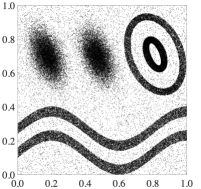
Figure 1: Two-dimensional synthetic dataset.

(a) Stream #1

(b) Stream #2

(c) Stream #3

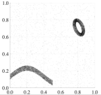
(d) Stream #4

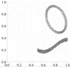
(e) Stream #5

(f) Stream #6

Figure 2: Visualization of the synthetic dataset in sequential order (i.e., (a) to (f)).

5.2 Evaluation by using Synthetic Dataset

First, we evaluate the clustering performance of CAE by using a two-dimensional synthetic dataset in the stationary and non-stationary environments.

5.2.1 Dataset

Fig. 1 shows the entire dataset in the stationary environment. The value range of each dimension is [0, 1]. The dataset has six distributions, each of which consist of 15,000 data points. In addition, 10% of uniformly distributed noise data points are added (1,500$\times$6 noise points in total). Fig. 2 shows the dataset in the non-stationary environment where data points in Fig. 1 are divided into six streams. Each stream is given in sequential order as in streams #1 to #6. During our experiments, the data points in each dataset are presented to each algorithm only once without pre-processing. In the stationary environment, the data points are randomly selected from the entire dataset. In the non-stationary environment, the data points are randomly selected from a specific distribution in the dataset, and the cldistributionass is shifted sequentially. Since CAE is a clustering algorithm, we use the same data points for training and testing, i.e., an algorithm is trained by all the data points of a dataset and tested by the same data points as the training data.

TABLE III: Parameter specifications by grid search for synthetic dataset

Environment	AutoCloud	ASOINN		TCA		CAEA
	$m$	$\lambda$	$a_{\mathrm{max}}$	$\lambda$	$\sigma_{\mathrm{init}}$	$\lambda$	$a_{\mathrm{max}}$
Stationary	2	400	10	450	0.1	50	30
Non-stationary	2	250	10	500	0.1	50	40

(a) AutoCloud

(b) ASOINN

(c) SOINN+

(d) TCA

(e) CAEA

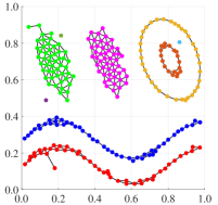
(f) CAE

Figure 3: Visualization of self-organizing results in the stationary environment.

5.2.2 Results

During grid search, each algorithm is trained by using all the data points, and calculating the Normalized Mutual Information (NMI) [54] score by using the same data points as training. We repeat the evaluation 15 times with data points selected by different random seeds. The result of the parameter setting that gives the median NMI score among 15 runs is used for comparison. Table III summarizes the results of grid search for synthetic dataset. It can be seen that the parameter values for each algorithm are depending on the environment.

Fig. 3 shows the visualization of self-organizing results in the stationary environment. The figures are the results of the trial in which a median NMI is obtained. AutoCloud creates and merges data clouds (i.e., cluster-like granular structures) without edge information, and thus the clustering result seems different from all the other algorithms. In addition, AutoCloud is originally proposed as an online learning algorithm. Therefore, the clustering result in the stationary environment is not well-organized. ASOINN and SOINN+ tend to create disconnected topological networks. On the other hand, thanks to properties of ART-based algorithms (e.g., a fixed similarity threshold value), TCA, CAEA, and CAE successfully define well-organized topological networks. Comparing CAE with TCA and CAEA, TCA and CAEA tend to generate a larger number of nodes than CAE. In Fig. 3, we can also see that there are some isolated nodes in CAE. This is because the number of presented data points is, in general, not a multiple of the deletion cycle (i.e., because the deletion process in line 14 of Algorithm 1 is, in general, not applied just before the termination of the algorithm for performance evaluation). This phenomenon also exists in SOINN+ (see Fig. 6). Moreover, the same phenomenon is also observed in TCA and CAEA depending on the deletion cycle of isolated nodes. A simple solution for avoiding this phenomenon is to delete isolated nodes after the learning procedure. However, since these algorithms aim for continual learning, they prepare for future learning without removing isolated nodes after the current learning procedure. Therefore, we consider that this is not a drawback for these algorithms.

(a) Stream #1

(b) Stream #2

(c) Stream #3

(d) Stream #4

(e) Stream #5

(f) Stream #6

Figure 4: Visualization of self-organizing results of AutoCloud in the non-stationary environment.

(a) Stream #1

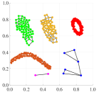
(b) Stream #2

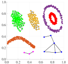
(c) Stream #3

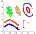
(d) Stream #4

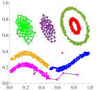
(e) Stream #5

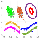
(f) Stream #6

Figure 5: Visualization of self-organizing results of ASOINN in the non-stationary environment.

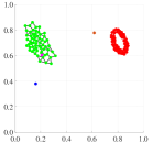
(a) Stream #1

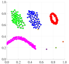
(b) Stream #2

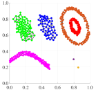
(c) Stream #3

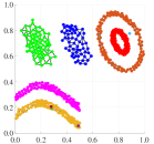
(d) Stream #4

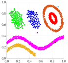
(e) Stream #5

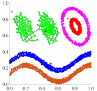
(f) Stream #6

Figure 6: Visualization of self-organizing results of SOINN+ in the non-stationary environment.

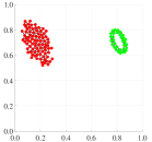
(a) Stream #1

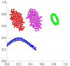
(b) Stream #2

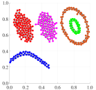
(c) Stream #3

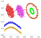
(d) Stream #4

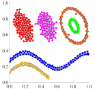
(e) Stream #5

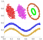
(f) Stream #6

Figure 7: Visualization of self-organizing results of TCA in the non-stationary environment.

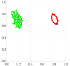
(a) Stream #1

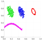
(b) Stream #2

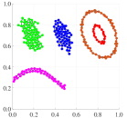
(c) Stream #3

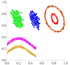
(d) Stream #4

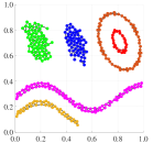
(e) Stream #5

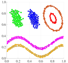
(f) Stream #6

Figure 8: Visualization of self-organizing results of CAEA in the non-stationary environment.

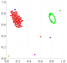
(a) Stream #1

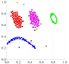
(b) Stream #2

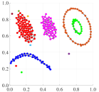
(c) Stream #3

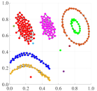
(d) Stream #4

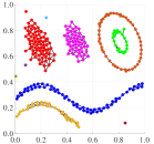
(e) Stream #5

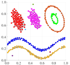
(f) Stream #6

Figure 9: Visualization of self-organizing results of CAE in the non-stationary environment.

TABLE IV: Results of quantitative comparisons on the synthetic dataset in the stationary environment

Metric	AutoCloud	ASOINN	SOINN+	TCA	CAEA	CAE
NMI	0.000 (0.000)	0.977 (0.022)	0.905 (0.077)	0.998 (0.000)	0.998 (0.000)	0.907 (0.254)
ARI	0.000 (0.000)	0.959 (0.058)	0.811 (0.178)	0.999 (0.000)	0.999 (0.000)	0.868 (0.270)
# of Nodes	—	373.5 (14.5)	451.7 (88.5)	488.3 (6.8)	432.3 (82.3)	243.1 (34.4)
# of Clusters	2.0 (0.0)	6.4 (0.8)	10.8 (3.4)	6.1 (0.3)	6.0 (0.0)	7.0 (2.4)

The values in parentheses indicate the standard deviation.

TABLE V: Results of quantitative comparisons on the synthetic dataset in the non-stationary environment

Dataset	Metric	AutoCloud	ASOINN	SOINN+	TCA	CAEA	CAE
Stream #1	NMI	0.067 (0.258)	0.800 (0.414)	0.980 (0.018)	0.998 (0.006)	1.000 (0.000)	0.987 (0.015)
	ARI	0.067 (0.258)	0.800 (0.414)	0.990 (0.010)	0.999 (0.003)	1.000 (0.000)	0.993 (0.008)
	# of Nodes	—	243.4 (16.1)	150.9 (48.6)	125.1 (4.1)	85.2 (11.9)	86.2 (12.7)
	# of Clusters	1.2 (0.8)	1.8 (0.4)	5.8 (3.1)	2.1 (0.4)	2.0 (0.0)	5.5 (2.7)
Stream #2	NMI	0.540 (0.183)	0.806 (0.132)	0.967 (0.050)	0.997 (0.001)	0.995 (0.004)	0.992 (0.005)
	ARI	0.279 (0.109)	0.625 (0.235)	0.953 (0.100)	0.999 (0.001)	0.997 (0.003)	0.996 (0.003)
	# of Nodes	—	450.2 (27.5)	339.1 (111.2)	255.5 (10.2)	190.2 (24.0)	180.1 (28.2)
	# of Clusters	4.0 (1.5)	2.9 (0.7)	9.4 (4.8)	4.1 (0.4)	4.3 (0.5)	7.1 (2.6)
Stream #3	NMI	0.467 (0.119)	0.856 (0.093)	0.936 (0.080)	0.998 (0.000)	0.992 (0.010)	0.991 (0.013)
	ARI	0.176 (0.075)	0.687 (0.204)	0.876 (0.174)	0.999(0.000)	0.994 (0.011)	0.993 (0.013)
	# of Nodes	—	598.7 (30.6)	504.4 (151.4)	344.5 (16.6)	263.1 (37.2)	242.7 (44.3)
	# of Clusters	4.7 (0.5)	3.8 (0.9)	12.0 (4.5)	5.1 (0.3)	5.5 (0.6)	8.0 (2.6)
Stream #4	NMI	0.465 (0.110)	0.915 (0.076)	0.951 (0.053)	0.998 (0.000)	0.995(0.007)	0.994 (0.009)
	ARI	0.219 (0.079)	0.809 (0.172)	0.903 (0.122)	0.999 (0.000)	0.996 (0.007)	0.996 (0.008)
	# of Nodes	—	727.7 (32.4)	688.2 (207.6)	390.9 (19.8)	306.2 (45.7)	279.0 (54.0)
	# of Clusters	5.3 (0.9)	5.4 (0.8)	13.1 (5.8)	6.1 (0.3)	6.4 (0.5)	9.2 (2.6)
Stream #5	NMI	0.476 (0.590)	0.881 (0.133)	0.951 (0.026)	0.999 (0.000)	0.994 (0.014)	0.994 (0.014)
	ARI	0.267 (0.066)	0.748 (0.261)	0.909 (0.056)	0.999 (0.000)	0.991 (0.032)	0.990 (0.032)
	# of Nodes	—	864.7 (39.4)	855.3 (259.7)	438.3 (22.1)	352.1 (55.6)	315.9 (65.6)
	# of Clusters	5.2 (0.9)	5.9 (1.9)	15.0 (6)	6.0 (0.0)	6.1 (0.3)	8.0 (1.7)
Stream #6	NMI	0.470 (0.078)	0.891 (0.100)	0.941 (0.032)	0.999 (0.000)	0.998 (0.001)	0.988 (0.020)
	ARI	0.234 (0.093)	0.739 (0.221)	0.870 (0.083)	0.999 (0.000)	0.999 (0.000)	0.979 (0.047)
	# of Nodes	—	993.4 (41.8)	1063.3 (323.4)	492.1 (24.3)	406.0 (65.2)	359.9 (75.9)
	# of Clusters	5.4 (0.5)	6.7 (1.1)	17.7 (9.4)	6.0 (0.0)	6.1 (0.4)	8.5 (1.9)

The values in parentheses indicate the standard deviation.

Figs. 4-9 show the visualization of self-organizing results in the non-stationary environment. The figures are the results of the trial in which a median NMI is obtained. With respect to AutoCloud, the clustering performance is better than that in the stationary environment. However, it is difficult for AutoCloud to handle non-Gaussian distributions. ASOINN tends to generate topological networks by noise data points. Besides, ASOINN tends to generate much more nodes than that in the stationary environment. With respect to SOINN+, two clusters are eventually connected. In addition, as in the case of ASOINN, SOINN+ also tends to generate much more nodes than those in the stationary environment. In contrast, TCA, CAEA, and TCA generate topological networks that are similar to the results obtained in the stationary environment. In Fig. 9, although CAE creates several isolated nodes, each isolated node does not overlap with topological networks. On the other hand, Fig. 6 shows that the isolated nodes of SOINN+ overlap with topological networks, indicating that the networks are not properly generated.

Tables IV and V summarize the results for quantitative comparisons to the synthetic dataset in the stationary and non-stationary environments, respectively. Here, we compare the mean values of NMI, Adjusted Rand Index (ARI) [55], the number of nodes and clusters of each algorithm among 15 runs. Algorithm comparisons based on NMI and ARI (in Tables IV and V) show that the clustering performance of each algorithm is comparable in both environments. However, the number of nodes of ASOINN and SOINN+ is greatly different depending on the environment while TCA, CAEA, and CAE have a similar number of nodes in each environment.

The above-mentioned observations of the results in this section indicate that the stability of the self-organizing performance of TCA, CAEA, and CAE is superior to that of AutoCloud, ASOINN, and SOINN+.

5.3 Evaluation by using Real-world Datasets

Next, we indirectly evaluate the clustering performance of CAE via classification tasks, which use a clustering result as a classifier, on real-world datasets in the stationary and non-stationary environments.

TABLE VI: Statistics of real-world datasets

Dataset	# of	# of	# of
	Data Points	Attributes	Classes
Iris	150	4	3
Ionosphere	351	34	2
Pima	768	8	2
Yeast	1,484	8	10
Image Segmentation	2,310	19	7
Phoneme	5,404	5	2
Texture	5,500	40	11
PenBased	10,992	16	10
Letter	20,000	16	26
Skin	245,057	3	2

TABLE VII: Parameter specifications by grid search for real-world datasets in the stationary environment

Dataset	AutoCloud	ASOINN		TCA		CAEA
	$m$	$\lambda$	$a_{\mathrm{max}}$	$\lambda$	$\sigma_{\mathrm{init}}$	$\lambda$	$a_{\mathrm{max}}$
Iris	1	50	10	100	0.3	50	90
Ionosphere	1	500	10	400	0.2	400	10
Pima	1	450	50	500	0.2	400	70
Yeast	1	500	90	500	0.3	500	40
Image Seg.	1	100	20	50	0.2	100	20
Phoneme	1	50	10	150	0.2	500	90
Texture	1	200	10	250	0.2	500	100
PenBased	1	150	10	150	0.3	100	50
Letter	N/A	400	10	500	0.2	450	10
Skin	N/A	50	20	200	0.1	50	80
Mean parameter values for CAEA(mean)						306	56

Image Seg. stands for Image Segmentation.
  N/A indicates that an algorithm could not build a predictive model
  within 12 hours under the available computational resources.

TABLE VIII: Parameter specifications by grid search for real-world datasets in the non-stationary environment

Dataset	AutoCloud	ASOINN		TCA		CAEA
	$m$	$\lambda$	$a_{\mathrm{max}}$	$\lambda$	$\sigma_{\mathrm{init}}$	$\lambda$	$a_{\mathrm{max}}$
Iris	1	300	10	100	0.3	50	90
Ionosphere	1	500	10	500	0.2	350	70
Pima	1	400	50	350	0.2	300	60
Yeast	1	500	30	500	0.3	500	90
Image Seg.	1	200	20	50	0.2	100	60
Phoneme	1	500	10	150	0.2	400	30
Texture	1	350	10	150	0.2	200	90
PenBased	1	150	10	150	0.3	50	70
Letter	N/A	450	10	500	0.2	500	50
Skin	N/A	50	20	200	0.1	50	60
Mean parameter values for CAEA(mean)						250	67

Image Seg. stands for Image Segmentation.
  N/A indicates that an algorithm could not build a predictive model
  within 12 hours under the available computational resources.

5.3.1 Dataset

We use 10 real-world datasets from public repositories [56, 57]. Table VI summarizes statistics of the 10 real-world datasets. During our experiments, all data points in each dataset are presented to each algorithm only once without pre-processing. As in section 5.2.2, in the stationary environment, all data points in each dataset are presented to each algorithm in random order. In the non-stationary environment, the data points are randomly selected from a specific class in the dataset, and the class is shifted sequentially. In addition, we use the same data points for training and testing, i.e., an algorithm is trained by all data points in each dataset and tested by the same data points as the training data. Note that the class information of each data point is not used in the training phase.

5.3.2 Results

During grid search, each algorithm is trained for each dataset by using all data points, and calculating the NMI score by using the same data points as training. In each parameter setting of grid search, we repeat the evaluation 20 times (i.e., 2$\times$10-fold cross validation) with different random seeds. The result of the parameter setting that gives the highest NMI score is used for comparisons. Tables VII and VIII summarize the results of grid search for real-world datasets in the stationary and non-stationary environments, respectively. It can be seen that the parameter values for each algorithm depend on the datasets and the environment. Note that the proposed CAE has no parameter to be pre-specified.

To emphasize the difficulty of using a single parameter specification for all datasets, we use CAEA with fixed parameter values, called CAEA(mean), as an additional compared algorithm. Tables VII and VIII show the parameter values of CAEA(mean) for the stationary and non-stationary environments, respectively. These parameters are specified by using the mean values of the parameters of CAEA over all datasets in each environment.

Tables IX and X show the results of classification performance on the 10 real-world datasets in the stationary and non-stationary environments, respectively. The best value in each metric is indicated by bold, and the values in parentheses indicate the standard deviation. A number to the right of each evaluation metric is the average rank of an algorithm over 20 evaluations. The smaller the rank, the better the metric score. In addition, a darker tone in a cell corresponds to a smaller rank (i.e., better evaluation). As general trends, CAEA shows better classification performance than the other algorithms. In contrast, the classification performance of CAEA(mean) deteriorates compared with CAEA. This indicates that CAEA is very sensitive to parameter specifications. Although CAE does not show the best value of NMI and ARI, it generally shows better clustering performance than the other algorithms except for CAEA with careful parameter specifications. The parameter-free algorithms (i.e., SOINN+ and CAE) tend to create a large number of nodes and clusters. In particular, SOINN+ creates a very large number of nodes and clusters when the number of data points is large (e.g., Skin dataset with 245,0057 data points). This is a disadvantage from the viewpoint of data aggregation/grouping, which is the general purpose of clustering. Since AutoCloud is specialized as an online learning algorithm, its classification performance is significantly low in the stationary environment. In addition, AutoCloud could not build a predictive model within 12 hours under the available computational resources in the case of datasets with a large number of data points (i.e., Letter and Skin datasets).

TABLE IX: Results of quantitative comparisons on 10 real-world datasets in the stationary environment

Dataset	Metric	AutoCloud	ASOINN	SOINN+	TCA	CAEA	CAEA (mean)	CAE
Iris	NMI	0.700 (0.094) 3.2	0.725 (0.171) 2.1	0.606 (0.048) 5.2	0.760 (0.004) 1.9	0.723 (0.045) 3.3	0.469 (0.000) 6.9	0.563 (0.056) 5.6
	ARI	0.529 (0.089) 3.5	0.557 (0.144) 2.9	0.442 (0.091) 4.9	0.572 (0.017) 2.7	0.661 (0.074) 1.4	0.000 (0.000) 7.0	0.217 (0.162) 5.7
	# of Nodes	—	11.3 (2.6)	26.4 (6.8)	10.1 (1.2)	20.6 (2.2)	150.0 (0.0)	52.0 (20.0)
	# of Clusters	3.0 (0.2)	2.1 (0.4)	10.0 (4.5)	2.1 (0.2)	5.2 (1.0)	150.0 (0.0)	36.5 (19.7)
Ionosphere	NMI	0.003 (0.008) 7.0	0.196 (0.072) 4.2	0.143 (0.055) 5.0	0.092 (0.054) 5.6	0.362 (0.012) 1.2	0.267 (0.022) 3.1	0.315 (0.022) 2.1
	ARI	0.000 (0.001) 6.8	0.131 (0.104) 2.8	0.083 (0.059) 3.8	0.063 (0.065) 4.3	0.067 (0.032) 4.4	0.080 (0.031) 3.7	0.126 (0.052) 2.4
	# of Nodes	—	43.4 (5.9)	26.0 (9.5)	12.9 (3.0)	263.1 (5.2)	56.8 (2.2)	122.8 (26.4)
	# of Clusters	1.3 (0.5)	9.7 (2.3)	11.8 (4.5)	3.7 (1.2)	206.2 (7.3)	104.5 (3.9)	76.5 (23.3)
Pima	NMI	0.003 (0.009) 6.7	0.010 (0.014) 6.1	0.039 (0.018) 4.7	0.044 (0.017) 4.4	0.186 (0.010) 1.2	0.129 (0.008) 2.7	0.156 (0.064) 2.4
	ARI	0.005 (0.019) 6.4	0.011 (0.010) 5.8	0.042 (0.022) 3.4	0.039 (0.029) 3.7	0.056 (0.016) 2.8	0.070 (0.013) 1.7	0.029 (0.020) 4.3
	# of Nodes	—	76.7 (12.4)	58.6 (15.6)	40.9 (5.5)	337.4 (11.5)	126.1 (6.9)	310.0 (148.6)
	# of Clusters	2.0 (0.0)	2.2 (0.6)	13.3 (6.3)	7.1 (2.1)	247.7 (12.2)	207.1 (7.2)	210.0 (140.8)
Yeast	NMI	0.003 (0.007) 6.5	0.037 (0.047) 5.8	0.076 (0.061) 4.9	0.080 (0.065) 4.8	0.331 (0.010) 1.0	0.287 (0.014) 2.3	0.225 (0.059) 2.9
	ARI	0.000 (0.000) 6.2	0.003 (0.004) 5.5	0.013 (0.032) 5.3	0.012 (0.021) 4.8	0.089 (0.014) 2.2	0.099 (0.021) 1.7	0.079 (0.031) 2.5
	# of Nodes	—	101.3 (12.9)	68.9 (27.0)	12.2 (2.6)	472.5 (15.8)	181.7 (9.2)	243.0 (105.2)
	# of Clusters	7.2 (1.3)	1.7 (1.0)	7.7 (5.3)	1.8 (0.6)	318.9 (16.4)	303.3 (11.3)	108.6 (81.9)
Image	NMI	0.342 (0.127) 7.0	0.632 (0.002) 3.2	0.554 (0.018) 5.9	0.641 (0.047) 2.6	0.663 (0.023) 1.6	0.599 (0.006) 4.9	0.637 (0.027) 2.9
Segmentation	ARI	0.115 (0.089) 6.7	0.236 (0.000) 4.6	0.252 (0.048) 4.5	0.437 (0.109) 2.0	0.486 (0.048) 1.7	0.218 (0.024) 5.6	0.383 (0.099) 3.0
	# of Nodes	—	42.2 (5.0)	128.2 (30.5)	30.7 (4.0)	77.8 (8.0)	132.6 (7.2)	122.7 (53.4)
	# of Clusters	7.0 (0.0)	3.0 (0.0)	22.7 (9.2)	5.2 (1.1)	19.8 (2.2)	258.3 (5.9)	49.3 (36.3)
Phoneme	NMI	0.020 (0.048) 6.4	0.048 (0.072) 5.5	0.037 (0.031) 5.3	0.117 (0.054) 3.5	0.174 (0.003) 1.3	0.160 (0.005) 2.7	0.154 (0.007) 3.5
	ARI	0.024 (0.069) 5.7	0.027 (0.053) 5.2	0.015 (0.023) 5.5	0.146 (0.054) 1.5	0.037 (0.015) 4.3	0.054 (0.018) 3.4	0.085 (0.031) 2.4
	# of Nodes	—	32.6 (3.3)	166.6 (47.7)	83.6 (4.8)	526.4 (11.7)	141.6 (9.4)	245.5 (48.9)
	# of Clusters	2.0 (0.0)	1.7 (0.9)	11.3 (5.6)	4.5 (1.1)	280.3 (12.5)	316.8 (9.2)	83.0 (42.5)
Texture	NMI	0.290 (0.099) 7.0	0.609 (0.040) 4.6	0.572 (0.049) 5.3	0.598 (0.003) 4.8	0.713 (0.016) 1.4	0.671 (0.015) 2.8	0.680 (0.046) 2.3
	ARI	0.063 (0.050) 6.8	0.164 (0.036) 5.0	0.158 (0.038) 5.2	0.148 (0.002) 4.9	0.568 (0.048) 1.3	0.462 (0.032) 2.5	0.471 (0.111) 2.4
	# of Nodes	—	91.4 (6.2)	163.7 (40.7)	59.4 (3.7)	262.8 (7.9)	207.5 (19.4)	175.1 (68.8)
	# of Clusters	10.1 (0.3)	4.4 (0.9)	18.7 (6.6)	4.1 (0.2)	25.8 (4.3)	372.1 (11.5)	59.3 (46.7)
PenBased	NMI	0.385 (0.018) 7.0	0.699 (0.062) 3.7	0.709 (0.068) 3.1	0.669 (0.061) 5.1	0.739 (0.015) 2.0	0.703 (0.013) 4.0	0.720 (0.016) 3.3
	ARI	0.151 (0.013) 7.0	0.476 (0.154) 4.1	0.492 (0.166) 3.6	0.397 (0.115) 5.4	0.647 (0.036) 1.4	0.540 (0.035) 3.9	0.597 (0.044) 2.7
	# of Nodes	—	88.4 (7.2)	273.4 (67.1)	87.2 (3.0)	178.9 (6.0)	178.9 (14.8)	382.4 (153.2)
	# of Clusters	10.0 (0.0)	7.9 (1.5)	32.2 (10.6)	7.7 (1.4)	50.2 (8.4)	420.0 (11.1)	112.5 (95.0)
Letter	NMI	N/A        7.0	0.150 (0.061) 5.5	0.153 (0.035) 5.5	0.430 (0.021) 3.7	0.499 (0.006) 1.5	0.444 (0.017) 3.1	0.491 (0.059) 1.8
	ARI	N/A        7.0	0.004 (0.004) 5.5	0.002 (0.001) 5.6	0.086 (0.021) 3.2	0.134 (0.010) 1.3	0.088 (0.021) 3.2	0.109 (0.035) 2.3
	# of Nodes	—	208.6 (14.3)	234.7 (53.0)	222.5 (14.6)	415.2 (25.0)	107.0 (11.1)	639.3 (223.5)
	# of Clusters	N/A	3.2 (1.2)	11.2 (5.3)	31.5 (3.5)	216.0 (15.4)	355.9 (24.01)	253.8 (179.0)
Skin	NMI	N/A        7.0	0.560 (0.082) 2.6	0.338 (0.016) 6.0	0.635 (0.020) 1.4	0.563 (0.044) 2.9	0.416 (0.026) 5.0	0.559 (0.057) 3.2
	ARI	N/A        7.0	0.553 (0.204) 3.1	0.081 (0.031) 6.0	0.713 (0.021) 1.7	0.674 (0.084) 2.4	0.277 (0.099) 5.0	0.653 (0.103) 2.9
	# of Nodes	—	100.6 (8.7)	1038.3 (263.6)	202.0 (7.1)	225.9 (32.4)	100.1 (11.3)	254.6 (53.1)
	# of Clusters	N/A	2.7 (1.0)	122.7 (33.8)	5.7 (1.4)	9.5 (2.2)	812.3 (23.0)	14.1 (6.4)
	Average Rank	6.386 (1.077)	4.367 (1.218)	4.914 (0.835)	3.589 (1.362)	2.013 (0.993)	3.728 (1.496)	3.004 (1.024)

The best value in each metric is indicated by bold. The values in parentheses indicate the standard deviation.
  A number to the right of a metric value is the average rank of an algorithm over 20 evaluations.
  The smaller the rank, the better the metric score. A darker tone in a cell corresponds to a smaller rank
  N/A indicates that an algorithm could not build a predictive model within 12 hours under the available computational resources.
  AutoCloud does not have a node thus it is indicated by a symbol “—”.

TABLE X: Results of quantitative comparisons on 10 real-world datasets in the non-stationary environment

Dataset	Metric	AutoCloud	ASOINN	SOINN+	TCA	CAEA	CAEA(mean)	CAE
Iris	NMI	0.775 (0.055) 1.7	0.724 (0.046) 2.5	0.609 (0.042) 4.4	0.761 (0.003) 1.9	0.590 (0.061) 4.7	0.479 (0.005) 6.4	0.460 (0.119) 6.5
	ARI	0.751 (0.095) 1.1	0.554 (0.072) 3.0	0.464 (0.112) 3.8	0.572 (0.019) 2.5	0.397 (0.073) 4.9	0.015 (0.013) 6.6	0.126 (0.151) 6.3
	# of Nodes	—	23.2 (3.9)	39.3 (8.3)	10.2 (0.8)	23.7 (5.8)	137.4 (3.6)	88.8 (56.0)
	# of Clusters	3.0 (0.0)	2.8 (0.8)	17.9 (6.2)	2.1 (0.2)	9.3 (1.8)	133.6 (6.1)	83.2 (58.8)
Ionosphere	NMI	0.045 (0.078) 6.5	0.204 (0.085) 4.0	0.169 (0.080) 4.5	0.118 (0.047) 5.7	0.397 (0.053) 1.4	0.304 (0.094) 2.5	0.246 (0.089) 3.5
	ARI	0.052 (0.092) 5.2	0.150 (0.133) 3.3	0.086 (0.076) 4.2	0.103 (0.064) 3.8	0.293 (0.257) 2.9	0.067 (0.056) 4.5	0.082 (0.077) 4.2
	# of Nodes	—	44 .0(5.0)	41.1 (10.7)	13.1 (3.5)	232.1 (64.5)	134.1 (8.8)	92.2 (32.5)
	# of Clusters	1.7 (0.5)	10.4 (3.3)	19.2 (8.5)	3.9 (1.5)	193.3 (76.3)	105.9 (3.7)	62.3 (31.1)
Pima	NMI	0.004 (0.014) 6.7	0.008 (0.010) 6.0	0.045 (0.018) 4.5	0.039 (0.027) 4.6	0.171 (0.053) 1.5	0.081 (0.012) 3.0	0.145 (0.062) 1.9
	ARI	0.003 (0.011) 6.4	0.011 (0.008) 5.6	0.050 (0.050) 4.2	0.053 (0.027) 3.3	0.051 (0.021) 3.3	0.105 (0.033) 1.5	0.050 (0.046) 4.2
	# of Nodes	—	80.6 (12.3)	66.9 (17.1)	31.4 (4.2)	342.6 (76.9)	109.5 (7.4)	288.6 (157.2)
	# of Clusters	2.0 (0.0)	2.3 (0.9)	15.6 (5.9)	4.4 (1.6)	246.4 (87.8)	29.4 (1.7)	210.4 (160.0)
Yeast	NMI	0.045 (0.054) 6.1	0.032 (0.042) 6.2	0.172 (0.055) 3.7	0.085 (0.042) 5.2	0.397 (0.021) 1.0	0.271 (0.029) 2.3	0.187 (0.091) 3.6
	ARI	0.009 (0.016) 5.7	0.003 (0.004) 6.1	0.042 (0.033) 3.9	0.011 (0.012) 5.3	0.082 (0.032) 2.2	0.098 (0.043) 2.0	0.073 (0.051) 3.0
	# of Nodes	—	101.2 (13.9)	196.4 (56.8)	12.4 (2.3)	888.9 (105.9)	283.7 (12.0)	216.1 (119.1)
	# of Clusters	10.0 (0.2)	1.6 (0.7)	46.9 (23.4)	2.1 (0.6)	711.5 (135.1)	174.7 (20.4)	95.4 (104.8)
Image	NMI	0.642 (0.037) 2.6	0.630 (0.007) 3.1	0.599 (0.013) 4.9	0.624 (0.055) 3.2	0.582 (0.060) 4.8	0.569 (0.028) 6.0	0.620 (0.051) 3.6
Segmentation	ARI	0.422 (0.086) 2.1	0.235 (0.004) 5.6	0.278 (0.065) 4.8	0.411 (0.114) 2.6	0.328 (0.083) 3.9	0.198 (0.063) 6.2	0.359 (0.106) 3.0
	# of Nodes	—	69.2 (7.4)	572.4 (64.5)	31.6 (4.3)	146.6 (38.6)	226.5 (20.3)	170.7 (46.6)
	# of Clusters	7.0 (0.0)	3.2 (0.4)	230.5 (48.4)	5.3 (1.6)	47.3 (11.5)	100.8 (15.5)	52.3 (30.2)
Phoneme	NMI	0.090 (0.052) 4.6	0.021 (0.014) 6.7	0.038 (0.010) 6.0	0.115 (0.050) 3.7	0.171 (0.015) 1.9	0.157 (0.008) 2.8	0.157 (0.013) 2.4
	ARI	0.169 (0.078) 2.1	0.004 (0.011) 6.7	0.016 (0.020) 6.0	0.149 (0.077) 2.2	0.052 (0.023) 4.4	0.054 (0.020) 4.0	0.096 (0.031) 2.8
	# of Nodes	—	188.7 (9.8)	248.8 (72.3)	82.3 (5.0)	496.0 (69.8)	309.5 (11.1)	274.5 (75.4)
	# of Clusters	2.0 (0.0)	2.5 (1.3)	21.8 (10.2)	4.9 (1.5)	251.1 (104.2)	114.4 (23.9)	83.4 (46.0)
Texture	NMI	0.602 (0.026) 5.5	0.621 (0.051) 4.6	0.665 (0.027) 2.9	0.591 (0.025) 6.0	0.667 (0.045) 2.7	0.681 (0.053) 2.3	0.632 (0.060) 4.1
	ARI	0.332 (0.074) 4.3	0.175 (0.043) 6.1	0.429 (0.069) 2.9	0.145 (0.014) 6.6	0.461 (0.093) 2.4	0.476 (0.124) 2.2	0.360 (0.144) 3.7
	# of Nodes	—	139.1 (9.1)	1400.3 (96.4)	51.3 (2.5)	462.2 (65.8)	527.3 (40.8)	520.8 (191.6)
	# of Clusters	11.0 (0.0)	4.9 (1.0)	483.3 (74.5)	4.0 (0.3)	112.7 (40.4)	63.8 (15.3)	164.3 (152.9)
PenBased	NMI	0.673 (0.025) 4.9	0.681 (0.055) 4.5	0.712 (0.025) 3.2	0.642 (0.096) 5.0	0.745 (0.050) 1.9	0.681 (0.074) 3.9	0.668 (0.068) 4.7
	ARI	0.511 (0.057) 3.9	0.402 (0.139) 5.3	0.565 (0.063) 3.0	0.346 (0.143) 6.0	0.626 (0.095) 2.0	0.506 (0.153) 3.6	0.452 (0.171) 4.4
	# of Nodes	—	91.1 (8.6)	2375.1 (158.0)	86.6 (3.8)	326.6 (44.7)	728.9 (144.8)	1006.4 (315.4)
	# of Clusters	10.0 (0.0)	7.6 (1.4)	713.3 (82.5)	7.0 (1.6)	23.2 (7.3)	175.6 (78.8)	260.9 (221.6)
Letter	NMI	N/A        7.0	0.168 (0.065) 6.0	0.590 (0.015) 1.0	0.441 (0.019) 4.7	0.502 (0.023) 2.8	0.475 (0.031) 3.9	0.517 (0.030) 2.7
	ARI	N/A        7.0	0.004 (0.003) 6.0	0.091 (0.020) 3.5	0.102 (0.029) 3.2	0.088 (0.007) 4.2	0.107 (0.012) 2.5	0.126 (0.025) 1.7
	# of Nodes	—	237.7 (9.8)	6059.2 (308.6)	229.2 (12.8)	1235.6 (171.6)	743.4 (173.5)	1062.3 (314.5)
	# of Clusters	N/A	4.5 (1.7)	2530.4 (315.4)	32.7 (3.6)	496.8 (28.9)	198.0 (27.4)	274.0 (120.3)
Skin	NMI	N/A        7.0	0.528 (0.087) 3.2	0.334 (0.023) 6.0	0.629 (0.016) 1.4	0.545 (0.048) 3.1	0.426 (0.052) 4.7	0.566 (0.060) 2.7
	ARI	N/A        7.0	0.471 (0.206) 3.6	0.081 (0.034) 6.0	0.712 (0.028) 1.8	0.645 (0.086) 2.7	0.380 (0.155) 4.6	0.662 (0.063) 2.5
	# of Nodes	—	92.6 (11.6)	1461.8 (402.0)	208.0 (9.1)	335.0 (53.1)	1036.1 (31.2)	376.1 (109.9)
	# of Clusters	N/A	3.0 (0.9)	144.6 (45.7)	6.5 (1.4)	15.1 (3.7)	55.6 (15.3)	17.0 (9.9)
	Average Rank	4.853 (1.944)	4.890 (1.352)	4.149 (1.250)	3.921 (1.553)	2.902 (1.159)	3.749 (1.551)	3.536 (1.229)

The best value in each metric is indicated by bold. The values in parentheses indicate the standard deviation.
  A number to the right of a metric value is the average rank of an algorithm over 20 evaluations.
  The smaller the rank, the better the metric score. A darker tone in a cell corresponds to a smaller rank
  N/A indicates that an algorithm could not build a predictive model within 12 hours under the available computational resources.
  AutoCloud does not have a node thus it is indicated by a symbol “—”.

For statistical comparisons, the Friedman test and Nemenyi post-hoc analysis [58] are used. The Friedman test is used to test the null hypothesis that all algorithms perform equally. If the null hypothesis is rejected, the Nemenyi post-hoc analysis is then conducted. The Nemenyi post-hoc analysis is used for all pairwise comparisons based on the ranks of results on each evaluation metric over all datasets. The difference in the performance between two algorithms is treated as statistically significant if the $p$-value defined by the Nemenyi post-hoc analysis is smaller than the significance level. Here, the null hypothesis is rejected at the significance level of $0.05$ both in the Friedman test and the Nemenyi post-hoc analysis.

Figs. 10-12 show critical difference diagrams based on results of NMI and ARI of each algorithm, which are defined by the Nemenyi post-hoc analysis. A better specification has lower average ranks, i.e., on the right side of each diagram. In theory, algorithms within a critical distance (i.e., a red line) do not have a statistically significance difference [58].

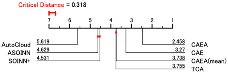
Figure 10: Critical difference diagram based on the overall results of NMI and ARI.

Fig. 10 shows a critical difference diagram based on the overall results (i.e., all the results of NMI and ARI in the stationary and non-stationary environments). CAEA is the lowest rank (i.e., best) algorithm with a statistically significant difference. However, the rank of CAEA(mean) is greatly deteriorated compared with CAEA. CAE is the best algorithm with a statistically significant difference among parameter-free/fixed algorithms (i.e., SOINN+ and CAEA(mean)). Moreover, CAE shows a lower rank with a statistically significant difference than ASOINN, TCA, and AutoCloud whose parameters specified by grid search.

In order to discuss the features of each algorithm in detail, Figs. 11 and 12 show critical difference diagrams based on the results of the stationary and non-stationary environments, respectively. With respect to CAEA, CAE, and TCA, these algorithms generally show lower ranks in both environments. On the other hand, SOINN+ and CAEA(mean) are less stable algorithms because their results vary greatly depending on the environment.

The above-mentioned observations suggest that although CAEA performs better than CAE, the superiority of CAE is demonstrated by its high and stable clustering performance on various datasets without specifying any parameters.

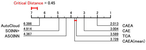
Figure 11: Critical difference diagram based on results of NMI and ARI in the stationary environment.

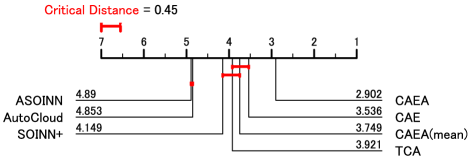
Figure 12: Critical difference diagram based on results of NMI and ARI in the non-stationary environment.

5.4 Validity of the Number of Active Nodes

From the experiments with the synthetic and real-world datasets, it can be considered that CAE has a superior clustering performance to the state-of-the-art parameter-free/fixed algorithms (i.e., SOINN+ and CAEA(mean)). In general for self-organizing clustering algorithms, a good specification of the similarity threshold provides good clustering performance. In CAE, the number of active nodes $\lambda$ plays an important role in the calculation of the similarity threshold, which is estimated by the DPP-based criterion incorporating CIM.

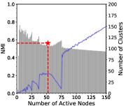
(a) Iris

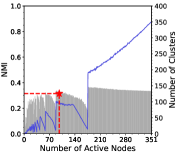
(b) Ionosphere

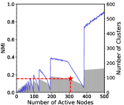
(c) Pima

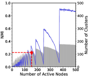
(d) Yeast

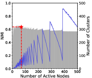
(e) Image Segmentation

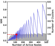
(f) Phoneme

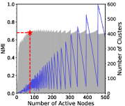
(g) Texture

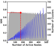
(h) PenBased

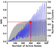
(i) Letter

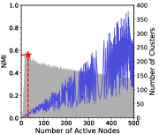
(j) Skin

Figure 13: Relationships among the number of active nodes, the number of clusters in CAE, and NMI in the stationary environment.

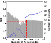
(a) Iris

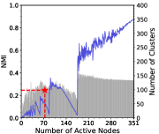
(b) Ionosphere

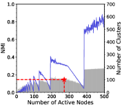
(c) Pima

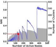
(d) Yeast

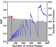
(e) Image Segmentation

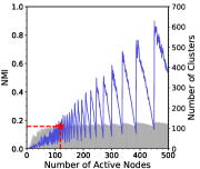
(f) Phoneme

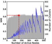
(g) Texture

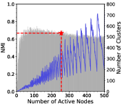
(h) PenBased

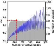
(i) Letter

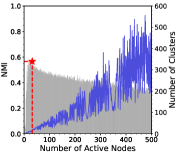
(j) Skin

Figure 14: Relationships among the number of active nodes, the number of clusters in CAE, and NMI in the non-stationary environment.

This section analyzes and discusses the validity of the number of active nodes, and its effect to clustering performance (i.e., NMI) and the number of clusters in CAE. First, we manually set the value of $\lambda$ (i.e., the number of active nodes), and then perform the training process of CAE without the specification process of $\ \lambda$. Then, we evaluate a trained network for obtaining a NMI value. The rest of the experimental settings is the same as in section 5.3. Figs. 13 and 14 show the relationships among the number of active nodes, NMI, and the number of clusters of each dataset in the stationary and non-stationary environments, respectively. A gray bar represents a value of NMI, and a blue line represents the number of clusters, respectively. In addition, a red star represents the estimated number of active nodes by a DPP-based criterion incorporating CIM.

Note that in Figs. 13 and 14, the number of clusters in each dataset is oscillating. The reason for this phenomenon is as follows: in the case that the deletion cycle of isolated nodes (i.e., the number of active nodes $\lambda$) is a multiple of the number of presented data points, there is no isolated node as clusters after training. In contrast, in the case that the deletion cycle $\lambda$ is not a multiple of the number of presented data points, at most $(\lambda-1)$ isolated nodes are remaining as clusters after training. As mentioned in section 5.2.2, a simple solution for avoiding this phenomenon is to delete isolated nodes after the learning procedure. However, since these algorithms aim for continual learning, they prepare for future learning without removing isolated nodes after the current learning procedure. Therefore, we consider that this is not a drawback for those algorithms.

As the general purpose of clustering (i.e., data aggregation/grouping), the desired result is high NMI value with a small number of clusters. From this perspective, in Figs. 13 and 14, the estimation of the number of active nodes is well-performed except for Iris dataset. Especially, the estimated number of active nodes for Ionosphere, Image Segmentation, Phoneme, Texture, and Skin datasets archive the almost highest NMI value both in the stationary and non-stationary environments.

The above-mentioned observations suggest that the DPP-based criterion incorporating CIM and the calculation of the similarity threshold $V_{\text{threshold}}$ as in (11) practically works well on various datasets.

5.5 Computational Complexity

For computational complexity analysis, we use the notations in Table I, namely $d$ is the dimensionality of a data point, $n$ is the number of data points, $K$ is the number of nodes, $\lambda$ is the number of active nodes, and $|\mathcal{E}|$ is the number of elements in the ages of edges set $\mathcal{E}$.

The computational complexity of each process in CAE is as follows: for computing a bandwidth of a kernel function in CIM is $\mathcal{O}(d)$, for computing CIM is $\mathcal{O}(ndK)$ (line 9 in Alg. 1), for sorting the results of CIM is $\mathcal{O}(K\log{K})$ (line 9 in Alg. 1), for calculating a pairwise similarity matrix by using CIM is $\mathcal{O}((\frac{\lambda}{2})^{2}dK)$ (line 1 in Alg. 2), for calculating determinant of the pairwise similarity matrix is $\mathcal{O}((\frac{\lambda}{2})^{3})$ (line 2 in Alg. 2), and for estimating the edge deletion threshold is $\mathcal{O}(|\mathcal{E}|\log{|\mathcal{E}|})$ (Alg. 4).

In general, $\lambda\ll n$, $K\ll n$, and $\lambda<K$. As a result, the computational complexity of CAE is $\mathcal{O}(ndK)$.

6 Concluding Remarks

This paper proposed a new parameter-free ART-based topological clustering algorithm capable of continual learning by introducing two parameter estimation processes, namely the estimation of the number of active nodes for calculating a similarity threshold by a DPP-based criterion incorporating CIM, and the estimation of a node deletion threshold based on the age of each edge. Empirical studies with the synthetic and real-world datasets showed that the clustering performance of CAE is superior to the state-of-the-art parameter-free/fixed algorithms while maintaining continual learning ability. Thanks to the capabilities of CAE, therefore, we can expect the high utility and potential of CAE as a data preprocessing method in various applications.

In real-world applications related to health, finance, and medical fields, a dataset often contains numerical and categorical attributes simultaneously. Such a dataset is called a mixed dataset [59]. A future research topic is to develop a parameter-free clustering algorithm that can handle a mixed dataset while maintaining continual learning capabilities.

Naoki Masuyama (S’12–M’16) received the B.Eng. degree from Nihon University, Funabashi, Japan, in 2010, the M.E. degree from Tokyo Metropolitan University, Hino, Japan in 2012, and the Ph.D. degree from the Faculty of Computer Science and Information Technology, University of Malaya, Kuala Lumpur, Malaysia, in 2016. He is currently an Associate Professor with the Department of Core Informatics, Graduate School of Informatics, Osaka Metropolitan University, Sakai, Japan. His current research interests include clustering, data mining, and continual learning.

Takanori Takebayashi received the B.S degree in Computer Science from Osaka Prefecture University, Japan in 2023. He is now a master course student in Department of informatics, Osaka Metropolitan University. His research interests include clustering, continual learning.

Yusuke Nojima received the B.S. and M.S. Degrees in mechanical engineering from Osaka Institute of Technology, Osaka, Japan, in 1999 and 2001, respectively, and the Ph.D. degree in system function science from Kobe University, Hyogo, Japan, in 2004. Since 2004, he has been with Osaka Prefecture University, Osaka, Japan, where he was a Professor in Department of Computer Science and Intelligent Systems from October 2020. From April 2022, he is a Professor in Department of Core Informatics, Graduate School of Informatics, Osaka Metropolitan University. His research interests include evolutionary fuzzy systems, evolutionary multiobjective optimization, and multiobjective data mining. He was a guest editor for several special issues in international journals. He was a task force chair on Evolutionary Fuzzy Systems in Fuzzy Systems Technical Committee of IEEE Computational Intelligence Society. He was an associate editor of IEEE Computational Intelligence Magazine (2014-2019).

Chu Kiong Loo (SM’14) holds a Ph.D. (University Sains Malaysia) and B.Eng. (First Class Hons in Mechanical Engineering from the University of Malaya). He was a Design Engineer in various industrial firms and is the founder of the Advanced Robotics Lab. at the University of Malaya. He has been involved in the application of research into Perus’s Quantum Associative Model and Pribram’s Holonomic Brain Model in humanoid vision projects. Currently, he is Professor of Computer Science and Information Technology at the University of Malaya, Malaysia. He has led many projects funded by the Ministry of Science in Malaysia and the High Impact Research Grant from the Ministry of Higher Education, Malaysia. Loo’s research experience includes brain-inspired quantum neural networks, constructivism-inspired neural networks, synergetic neural networks and humanoid research.

Hisao Ishibuchi (M’93–SM’10–F’14) received the B.S. and M.S. degrees in precision mechanics from Kyoto University, Kyoto, Japan, in 1985 and 1987, respectively, and the Ph.D. degree in computer science from Osaka Prefecture University, Sakai, Osaka, Japan, in 1992. Since 1987, he has been with Osaka Prefecture University for 30 years. He is currently a Chair Professor with the Department of Computer Science and Engineering, Southern University of Science Technology, Shenzhen, China. His current research interests include fuzzy rule-based classifiers, evolutionary multiobjective optimization, many-objective optimization, and memetic algorithms. Dr. Ishibuchi was the IEEE Computational Intelligence Society (CIS) VicePresident for Technical Activities from 2010 to 2013. He was an IEEE CIS AdCom Member from 2014 to 2019, and from 2021 to 2023, an IEEE CIS Distinguished Lecturer from 2015 to 2017, and from 2021 to 2023, and the Editor-in-Chief of the IEEE Computational Intelligence Magazine from 2014 to 2019. He is also an Associate Editor of the ACM Computing Survey, the IEEE Transactions ON Cybernetics, and the IEEE Access.

Stefan Wermter (Member, IEEE) is currently a Full Professor with the University of Hamburg, Hamburg, Germany, where he is also the Director of the Knowledge Technology Institute at the Department of Informatics. Currently, he is the co-coordinator of the International Collaborative Research Centre on Crossmodal Learning (TRR-169) and a coordinator of the European Training Network TRAIL on transparent interpretable robots. His main research interests are in the fields of neural networks, hybrid knowledge technology, cognitive robotics and human–robot interaction. He is an Associate Editor of Connection Science and International Journal for Hybrid Intelligent Systems. He is on the Editorial Board of the journals Cognitive Systems Research, Cognitive Computation and Journal of Computational Intelligence. He is serving as President for the European Neural Network Society.

References

- [1] S. Lloyd, “Least squares quantization in PCM,” IEEE Transactions on Information Theory, vol. 28, no. 2, pp. 129–137, 1982.
- [2] G. J. McLachlan, S. X. Lee, and S. I. Rathnayake, “Finite mixture models,” Annual Review of Statistics and its Application, vol. 6, pp. 355–378, 2019.
- [3] T. Kohonen, “Self-organized formation of topologically correct feature maps,” Biological Cybernetics, vol. 43, no. 1, pp. 59–69, 1982.
- [4] B. Fritzke, “A growing neural gas network learns topologies,” Advances in Neural Information Processing Systems, vol. 7, pp. 625–632, 1995.
- [5] F. Shen and O. Hasegawa, “A fast nearest neighbor classifier based on self-organizing incremental neural network,” Neural Networks, vol. 21, no. 10, pp. 1537–1547, 2008.
- [6] W. H. Chin, Y. Toda, N. Kubota, C. K. Loo, and M. Seera, “Episodic memory multimodal learning for robot sensorimotor map building and navigation,” IEEE Transactions on Cognitive and Developmental Systems, vol. 11, no. 2, pp. 210–220, June 2018.
- [7] G. I. Parisi, J. Tani, C. Weber, and S. Wermter, “Lifelong learning of spatiotemporal representations with dual-memory recurrent self-organization,” Frontiers in Neurorobotics, vol. 12, # 78, November 2018.
- [8] G. A. Carpenter and S. Grossberg, “The ART of adaptive pattern recognition by a self-organizing neural network,” Computer, vol. 21, no. 3, pp. 77–88, 1988.
- [9] G. A. Carpenter, S. Grossberg, and D. B. Rosen, “Fuzzy ART: Fast stable learning and categorization of analog patterns by an adaptive resonance system,” Neural Networks, vol. 4, no. 6, pp. 759–771, 1991.
- [10] S. Grossberg, Conscious Mind, Resonant Brain: How Each Brain Makes a Mind. Oxford University Press, June 2021. [Online]. Available: https://doi.org/10.1093/oso/9780190070557.001.0001
- [11] N. Masuyama, C. K. Loo, H. Ishibuchi, N. Kubota, Y. Nojima, and Y. Liu, “Topological clustering via adaptive resonance theory with information theoretic learning,” IEEE Access, vol. 7, pp. 76 920–76 936, 2019.
- [12] N. Masuyama, N. Amako, Y. Yamada, Y. Nojima, and H. Ishibuchi, “Adaptive resonance theory-based topological clustering with a divisive hierarchical structure capable of continual learning,” arXiv preprint arXiv:2201.10713, 2022.
- [13] W. Liu, P. P. Pokharel, and J. C. Príncipe, “Correntropy: Properties and applications in non-Gaussian signal processing,” IEEE Transactions on Signal Processing, vol. 55, no. 11, pp. 5286–5298, 2007.
- [14] B. Vigdor and B. Lerner, “The Bayesian ARTMAP,” IEEE Transactions on Neural Networks, vol. 18, no. 6, pp. 1628–1644, 2007.
- [15] L. Wang, H. Zhu, J. Meng, and W. He, “Incremental local distribution-based clustering using Bayesian adaptive resonance theory,” IEEE Transactions on Neural Networks and Learning Systems, vol. 30, no. 11, pp. 3496–3504, 2019.
- [16] N. Masuyama, Y. Nojima, C. K. Loo, and H. Ishibuchi, “Multi-label classification via adaptive resonance theory-based clustering,” IEEE Transactions on Pattern Analysis and Machine Intelligence, pp. 1–18, 2022.
- [17] A. Kulesza and B. Taskar, “Determinantal point processes for machine learning,” Foundations and Trends® in Machine Learning, vol. 5, no. 2–3, pp. 123–286, 2012.
- [18] J. Parker-Holder, A. Pacchiano, K. Choromanski, and S. Roberts, “Effective diversity in population based reinforcement learning,” in Proceedings of the 34th International Conference on Neural Information Processing Systems, ser. NIPS’20, no. 1515. Red Hook, NY, USA: Curran Associates Inc., December 2020, pp. 18 050–18 062.
- [19] C. Wiwatcharakoses and D. Berrar, “SOINN+, a self-organizing incremental neural network for unsupervised learning from noisy data streams,” Expert Systems with Applications, vol. 143, p. 113069, 2020.
- [20] G. M. Van de Ven and A. S. Tolias, “Three scenarios for continual learning,” arXiv preprint arXiv:1904.07734, 2019.
- [21] F. Wiewel and B. Yang, “Localizing catastrophic forgetting in neural networks,” arXiv preprint arXiv:1906.02568, 2019.
- [22] S. Marsland, J. Shapiro, and U. Nehmzow, “A self-organising network that grows when required,” Neural Networks, vol. 15, no. 8, pp. 1041–1058, 2002.
- [23] L. E. B. da Silva, I. Elnabarawy, and D. C. Wunsch II, “Distributed dual vigilance fuzzy adaptive resonance theory learns online, retrieves arbitrarily-shaped clusters, and mitigates order dependence,” Neural Networks, vol. 121, pp. 208–228, 2020.
- [24] N. Masuyama, C. K. Loo, and F. Dawood, “Kernel Bayesian ART and ARTMAP,” Neural Networks, vol. 98, pp. 76–86, 2018.
- [25] N. Masuyama, C. K. Loo, and S. Wermter, “A kernel Bayesian adaptive resonance theory with a topological structure,” International Journal of Neural Systems, vol. 29, no. 5, p. 1850052 (20 pages), 2019.
- [26] N. Masuyama, N. Amako, Y. Nojima, Y. Liu, C. K. Loo, and H. Ishibuchi, “Fast topological adaptive resonance theory based on correntropy induced metric,” in Proceedings of IEEE Symposium Series on Computational Intelligence, 2019, pp. 2215–2221.
- [27] L. E. B. da Silva, I. Elnabarawy, and D. C. Wunsch II, “Dual vigilance fuzzy adaptive resonance theory,” Neural Networks, vol. 109, pp. 1–5, January 2019.
- [28] L. E. B. da Silva and D. C. Wunsch, “Validity index-based vigilance test in adaptive resonance theory neural networks,” in in Proccedings of IEEE Symposium Series on Computational Intelligence. IEEE, 2017, pp. 1–8.
- [29] L. Meng, A.-H. Tan, and D. C. Wunsch, “Adaptive scaling of cluster boundaries for large-scale social media data clustering,” IEEE Transactions on Nneural Networks and Learning Systems, vol. 27, no. 12, pp. 2656–2669, December 2015.
- [30] V. Badrinarayanan, A. Kendall, and R. Cipolla, “Segnet: A deep convolutional encoder-decoder architecture for image segmentation,” IEEE Transactions on Pattern Analysis and Machine Intelligence, vol. 39, no. 12, pp. 2481–2495, January 2017.
- [31] T. Hinz, S. Heinrich, and S. Wermter, “Semantic object accuracy for generative text-to-image synthesis,” IEEE Transactions on Ppattern Analysis and Machine Intelligence, vol. 44, no. 3, pp. 1552–1565, September 2020.
- [32] K. Han, Y. Wang, H. Chen, X. Chen, J. Guo, Z. Liu, Y. Tang, A. Xiao, C. Xu, Y. Xu et al., “A survey on vision transformer,” IEEE Transactions on Pattern Analysis and Machine Intelligence, vol. 45, no. 1, pp. 87–110, February 2022.
- [33] E. Belouadah, A. Popescu, and I. Kanellos, “A comprehensive study of class incremental learning algorithms for visual tasks,” Neural Networks, vol. 135, pp. 38–54, March 2021.
- [34] F. Zenke, B. Poole, and S. Ganguli, “Continual learning through synaptic intelligence,” in Proceedings of International Conference on Machine Learning, 2017, pp. 3987–3995.
- [35] H. Shin, J. K. Lee, J. Kim, and J. Kim, “Continual learning with deep generative replay,” in Proceedings of the 31st International Conference on Neural Information Processing Systems, 2017, pp. 2994–3003.
- [36] C. V. Nguyen, Y. Li, T. D. Bui, and R. E. Turner, “Variational continual learning,” in Proceedings of International Conference on Learning Representations, 2018, pp. 1–18.
- [37] J. Kirkpatrick, R. Pascanu, N. Rabinowitz, J. Veness, G. Desjardins, A. A. Rusu, K. Milan, J. Quan, T. Ramalho, A. Grabska-Barwinska et al., “Overcoming catastrophic forgetting in neural networks,” Proceedings of the National Academy of Sciences, vol. 114, no. 13, pp. 3521–3526, March 2017.
- [38] G. A. Tahir and C. K. Loo, “An open-ended continual learning for food recognition using class incremental extreme learning machines,” IEEE Access, vol. 8, pp. 82 328–82 346, May 2020.
- [39] Y. Kongsorot, P. Horata, and P. Musikawan, “An incremental kernel extreme learning machine for multi-label learning with emerging new labels,” IEEE Access, vol. 8, pp. 46 055–46 070, 2020.
- [40] T. T. Nguyen, M. T. Dang, A. V. Luong, A. W.-C. Liew, T. Liang, and J. McCall, “Multi-label classification via incremental clustering on an evolving data stream,” Pattern Recognition, vol. 95, pp. 96–113, 2019.
- [41] L. Sun, X. Qin, W. Ding, J. Xu, and S. Zhang, “Density peaks clustering based on k-nearest neighbors and self-recommendation,” International Journal of Machine Learning and Cybernetics, vol. 12, pp. 1913–1938, March 2021.
- [42] W. Ma, X. Tu, B. Luo, and G. Wang, “Semantic clustering based deduction learning for image recognition and classification,” Pattern Recognition, vol. 124, p. # 108440, April 2022.
- [43] G. A. Carpenter, S. Grossberg, N. Markuzon, J. H. Reynolds, and D. B. Rosen, “Fuzzy ARTMAP: A neural network architecture for incremental supervised learning of analog multidimensional maps,” IEEE Transactions on Neural Networks, vol. 3, no. 5, pp. 698–713, 1992.
- [44] C. G. Bezerra, B. S. J. Costa, L. A. Guedes, and P. P. Angelov, “An evolving approach to data streams clustering based on typicality and eccentricity data analytics,” Information Sciences, vol. 518, pp. 13–28, May 2020.
- [45] C. Wiwatcharakoses and D. Berrar, “A self-organizing incremental neural network for continual supervised learning,” Expert Systems with Applications, vol. 185, p. 115662, 2021.
- [46] S. C. Tan, J. Watada, Z. Ibrahim, and M. Khalid, “Evolutionary fuzzy ARTMAP neural networks for classification of semiconductor defects,” IEEE Transactions on Neural Networks and Learning Systems, vol. 26, no. 5, pp. 933–950, 2014.
- [47] A. L. Matias and A. R. R. Neto, “OnARTMAP: A fuzzy ARTMAP-based architecture,” Neural Networks, vol. 98, pp. 236–250, 2018.
- [48] A. L. Matias, A. R. R. Neto, C. L. C. Mattos, and J. P. P. Gomes, “A novel fuzzy ARTMAP with area of influence,” Neurocomputing, vol. 432, pp. 80–90, 2021.
- [49] L. E. B. da Silva, N. Rayapati, and D. C. Wunsch, “iCVI-ARTMAP: Using incremental cluster validity indices and adaptive resonance theory reset mechanism to accelerate validation and achieve multiprototype unsupervised representations,” IEEE Transactions on Neural Networks and Learning Systems, pp. 1–14, 2022.
- [50] ——, “Incremental cluster validity index-guided online learning for performance and robustness to presentation order,” IEEE Transactions on Neural Networks and Learning Systems, pp. 1–15, 2022.
- [51] R. Yelugam, L. E. B. da Silva, and D. C. Wunsch II, “Topological biclustering ARTMAP for identifying within bicluster relationships,” Neural Networks, vol. 160, pp. 34–49, March 2023.
- [52] D. J. Henderson and C. F. Parmeter, “Normal reference bandwidths for the general order, multivariate kernel density derivative estimator,” Statistics & Probability Letters, vol. 82, no. 12, pp. 2198–2205, 2012.
- [53] B. W. Silverman, Density Estimation for Statistics and Data Analysis. Routledge, 2018.
- [54] A. Strehl and J. Ghosh, “Cluster ensembles—A knowledge reuse framework for combining multiple partitions,” Journal of Machine Learning Research, vol. 3, pp. 583–617, December 2002.
- [55] L. Hubert and P. Arabie, “Comparing partitions,” Journal of Classification, vol. 2, no. 1, pp. 193–218, 1985.
- [56] J. Derrac, S. Garcia, L. Sanchez, and F. Herrera, “KEEL data-mining software tool: Data set repository, integration of algorithms and experimental analysis framework,” Journal of Multiple-Valued Logic and Soft Computing, vol. 17, pp. 255–287, 2011.
- [57] D. Dua and C. Graff, “UCI machine learning repository,” University of California, Irvine, School of Information and Computer Sciences, 2019. [Online]. Available: http://archive.ics.uci.edu/ml
- [58] J. Demšar, “Statistical comparisons of classifiers over multiple data sets,” Journal of Machine Learning Research, vol. 7, no. 1, pp. 1–30, 2006.
- [59] A. Ahmad and S. S. Khan, “Survey of state-of-the-art mixed data clustering algorithms,” IEEE Access, vol. 7, pp. 31 883–31 902, 2019.