Gravitational Redshift Detection from the Magnetic White Dwarf Harbored in RX J1712.6$-$2414

Abstract

Gravitational redshift is a fundamental parameter that allows us to determine the mass-to-radius ratio of compact stellar objects, such as black holes, neutron stars, and white dwarfs (WDs). In the X-ray spectra of the close binary system, RX J1712.6$-$2414, obtained from the Chandra High-Energy Transmission Grating observation, we detected significant redshifts for characteristic X-rays emitted from hydrogen-like magnesium, silicon ($\Delta E/E_{\rm rest}\sim 7\times 10^{-4}$), and sulfur ($\Delta E/E_{\rm rest}\sim 15\times 10^{-4}$) ions, which are over the instrumental absolute energy accuracy (${\Delta E/E_{\rm rest}\sim 3.3}\times 10^{-4}$). Considering some possible factors, such as Doppler shifts associated with the plasma flow, systemic velocity, and optical depth, we concluded that the major contributor to the observed redshift is the gravitational redshift of the WD harbored in the binary system, which is the first gravitational redshift detection from a magnetic WD. Moreover, the gravitational redshift provides us with a new method of the WD mass measurement by invoking the plasma-flow theory with strong magnetic fields in close binaries. Regardless of large uncertainty, our new method estimated the WD mass to be $M_{\rm WD}>0.9\,M_{\odot}$.

1 Introduction

Main-sequence (MS) stars having a mass of less than 8 $M_{\odot}$ will evolve into a white dwarf (WD), a compact object with a radius of the order of $10^{4}$ km. Besides, the WDs can be evolved into even by the MSs of more than 8 $M_{\odot}$ in binaries due to binary evolution. The WD is supported against its gravity by electron degeneracy pressure. The WD in a close binary system is fed by a mass accretion from its companion star. Hence, as the WD becomes more massive, its radius shrinks to reinforce the degeneracy pressure. However, the WD mass has an upper limit (Chandrasekhar mass $\sim$ $1.38$ $M_{\odot}$) where the degeneracy pressure no longer supports its gravity (Chandrasekhar, 1931). A WD exceeding the mass limit is expected to bring about an explosion called a type-Ia supernova or an accretion-induced collapse into a neutron star. Therefore, the mass is a key parameter of the WDs. The type-Ia supernovae are used to calculate the distances from our galaxy to their host galaxies, demonstrating the accelerating expansion of the Universe (Riess et al., 1998; Perlmutter et al., 1999).

A gravitational redshift enables us to directly measure the WD mass-radius ratio. In weak gravitational regime, the gravitational redshift can be written as

$$v_{g}=cz=\frac{c\Delta E}{E_{\rm obs}}\simeq\frac{c\Delta E}{E_{\rm rest}}=0.635\frac{M_{\odot}}{R_{\odot}}\,{\rm km\,s^{-1}},$$ (1)

where $c$ is the speed of the light, $z$ is the redshift parameter, $E_{\rm obs}$ and $E_{\rm rest}$ are observed and rest-frame energies, respectively, and $\Delta E\equiv-(E_{\rm obs}-E_{\rm rest})$. Since Einstein proposed three measurements to test the general relativity, one of which is to measure the gravitational redshift from stars (Einstein, 1916), the gravitational redshift has been employed to calculate the WD mass. For example, the gravitational redshift of the first WD Sirius B is $v_{g}=cz=c\times(2.688\pm 0.026)\times 10^{-4}=80.65\pm 0.77$ km s^-1 and thus the WD mass is $1.017\pm 0.025$ M_⊙ (Joyce et al., 2018). This technique has been applied for the WDs in the common proper motion binaries (Greenstein & Trimble, 1967; Koester, 1987; Silvestri et al., 2001), in binaries in which the motion of both constituent star were well determined (Sion et al., 1998; Long & Gilliland, 1999; Smith et al., 2006; Steeghs et al., 2007; van Spaandonk et al., 2010; Parsons et al., 2012, 2017; Joyce et al., 2018), or in an open cluster (Greenstein & Trimble, 1967; Wegner et al., 1989; Claver et al., 2001; Pasquini et al., 2019), where the Doppler shift can be precisely measured to break the degeneracy with the gravitational redshift. However, there is no detection report of the gravitational redshift from highly magnetized ($B\gtrsim$ 0.1 MG), spun-up ($P_{\rm spin}\lesssim 10^{3}$ s) WDs, or from a WD with the X-ray.

Magnetic cataclysmic variables (mCVs) harbors a highly-magnetized WD, which is often highly spun up via mass accretion. The cataclysmic variables (CVs) are close binaries consisting of a WD and a companion of late-type star (Mukai, 2017). In the CVs, the accreting gas from the companion brings the angular momentum to the WD, causing the WD spin-up and frequently forming the accretion disk around the WD. Furthermore, as WD shrinks caused by mass gain, its magnetic field should be strengthened (Das et al., 2013). Such a strong magnetic field either prevents the accretion disk from reaching the WD surface (intermediate polar: IP; Patterson 1994) or the prevents forming the accretion disk itself (polar; Cropper 1990). The accreting gas is captured along the magnetic field and accelerated by the WD potential to a velocity greater than the sound velocity. Hence, a standing shock forms near the WD surface. According to Rankine-Hugoniot relations, the post-shock gas is heated up to $\sim 10^{8}$ K, and then the gas is highly ionized. While the post-shock gas is descending to the WD, the plasma is cooled down by emitting X-rays. The electrons and ions are gradually recombined so that the hydrogen- and helium-like (H- and He-like) ions of various elements (e.g., neon (Ne), magnesium (Mg), silicon (Si), sulfur (S), Argon (Ar), and iron (Fe)) are produced. The recombined ions return to their ground states by emitting X-ray line emissions, as is indicated by observed X-ray spectra. The ratio of the line intensities is contingent upon the ion population in the plasma flow. The features in the X-ray spectra, such as the cut-off energy of the continuum spectra, line intensity ratio, and line energy shift caused by the Doppler shift and/or the gravitational redshift, allow us to measure the temperature, density, velocity, and gravitational potential in the post-shock plasma in principle, all of which are linked to the WD potential, that is, the WD mass.

RX J1712.6$-$2414, also known as V2400 Oph, is an IP that was discovered from the ROSAT All-Sky Survey (Buckley et al., 1995). Follow-up optical/near-infrared observation detected a circular polarization with the spin period of $927$ s, indicating WD’s relatively strong magnetic field of $\bigl{(}9$–$27\bigr{)}\times 10^{6}$ G and that we always see only one of the magnetic poles; the accretion flow onto this magnetic pole is nearly parallel to our line of sight. This IP has been known as a diskless IP since it does not show the $927$-s spin modulation in most cases but shows the synodic $1003$-s modulation in the X-ray. On the other hand, the spin modulation was observed in 2001 by XMM-Newton, and in 2005 and 2014 by Suzaku (Joshi et al., 2019). However, the best-fit spectral model parameters of the 2001 XMM-Newton observation are consistent with those of the 2000 XMM-Newton observation where the spin modulation was not detected (Joshi et al., 2019), which means the effect of whether the disk forms on the plasma flow structure is minor. We observed RX J1712.6$-$2414 by High-Energy Transmission Grating (HETG) of the Chandra observatory to investigate the velocity profile of the plasma in the accretion flow. The HETG spectra potentially allow us to measure the Doppler shift of $\sim 30$ km s^-1 (Ishibashi et al., 2006).

2 Observation and data reduction

We carried out the X-ray observation of RX J1712.6$-$2414 with Chandra in May 2020. Table 1 shows the observation log of RX J1712.6$-$2414. The observation was divided into six intervals with the following observation IDs: 21274, 23038, 23039, 23244, 23267, and 23268. The total exposure time was $169.15$ ks. The HETG modules were inserted between the X-ray optics and the CCD chips. The HETG consists of two independent gratings: the Medium Energy Grating (MEG) covers the 0.4-5.0 keV with an energy resolution $\Delta E/E\sim$ 1/300 at 2 keV, and the High Energy Grating (HEG) covers the 0.8-10 keV with $\Delta E/E\sim$ 200 at 6 keV. We chose the FAINT and Timed Exposure modes for the instrumental setup. First, applying the latest calibration files of the instruments (the 4.9.5 version), we reprocessed the observational data with CIAO v4.12 (Fruscione et al., 2006). We did not apply any filters to the data. After applying the barycentric correction, we then created the averaged X-ray spectra, following the instructions of the Chandra analysis.

Table 1: Chandra observations of RX J1712.6$-$2414

Observation ID	Exposure (ks)	Start date	Instrument
21274	24.7	2020-05-30 07:31:32	HETGa
23038	22.9	2020-05-29 03:35:56	HETGa
23039	37.6	2020-05-06 04:05:57	HETGa
23244	37.6	2020-05-06 21:24:29	HETGa
23267	24.7	2020-05-31 01:29:08	HETGa
3268	21.7	2020-05-31 18:53:25	HETGa
aHigh-Energy Transmission Grating

3 Analysis and result

Figure 1 shows X-ray HETG spectra around H-like K_α lines of Ne, Mg, Si, S, Ar, and Fe. We focused on these emission lines to measure each energy shift because they consist of only K_α1 and K_α2, whose intensity ratio is invariant to the plasma temperature or density, and can be easily separated from lines emitted by ions in the other states. To determine their energy centroids, we extracted the spectra in the energy ranges of $0.98$–$1.07$, $1.44$–$1.51$, $1.96$–$2.05$, $2.52$–$2.72$, $3.18$–$3.44$, and $6.85$–$7.10$ keV for Ne, Mg, Si, S, Ar, and Fe, respectively. We fitted a power-law function to the continuum and two Gaussians incorporating the redshift parameter (zgauss) to the H-like K_α1 and K_α2 lines by using Xspec (version 12.11.0; Arnaud 1996). The Gaussian centers were fixed at the rest-frame energies of K_α1 and K_α2 lines tabulated in Table 2 and their widths were fixed at 0. The redshift parameter was common to the H-like K_α1 and K_α2 for each ions, and left free to fit the model to the data. Their intensity ratio was fixed at the nominal of $I_{{\rm K}_{\alpha 1}}/I_{{\rm K}_{\alpha 2}}=2$. The energy ranges we selected were narrow; no photoelectric absorption was introduced.

While the energy shifts of the K_α lines from H-like Ne, Ar, and Fe ions are marginal because of insufficient photon statistics, those from H-like Mg, Si, and S ions are statistically constrained as shown in Table 2: $\Delta E/E_{\rm rest}=6.9_{-0.2}^{+0.0}\times 10^{-4}$ for Mg, $7.4_{-0.7}^{+0.0}\times 10^{-4}$ for Si, and $15.4_{-4.6}^{+5.5}\times 10^{-4}$ for S, which correspond to the line-of-sight velocities of $2.1_{-0.1}^{+0.0}\times 10^{2}$, $2.2_{-0.2}^{+0.0}\times 10^{2}$, and $4.6_{-1.4}^{+1.7}$ km s${}^{-1}\times 10^{2}$, respectively. The errors represent the statistical $90$% confidence level.

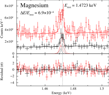
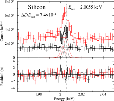
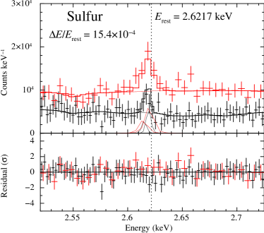
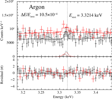
Figure 1: X-ray spectra obtained from the Chandra High Energy Grating (HEG; black) and Medium Energy Grating (MEG; red). We show the spectra including emission lines from H-like ions of Ne, Mg, Si, S, Ar, and Fe. The thick solid lines are the best-fit models. Meanwhile, the thin solid lines are the components of the best-fit models, consisting of a power-law function and two Gaussians. The residuals from the best-fit model are shown at the bottom of each panel. We also show the position of the rest-frame energy of each emission line by a vertical dotted line and the energy shift value.

Table 2: Summary of fitting to the H-like ion emission lines.

	Ne	Mg	Si	S	Ar	Fe
Significance ($\sigma$)	3.5	7.2	11.6	5.8	2.3	4.9
$E_{\rm rest}$ of Kα1 (keV)1	1.0220	1.4726	2.0061	2.6227	3.3230	6.9732
$E_{\rm rest}$ of Kα2 (keV)1	1.0215	1.4717	2.0043	2.6197	3.3182	6.9520
Energy centroid of Kα1 and Kα2 (keV)2	1.0218	1.4723	2.0055	2.6217	3.3214	6.9660
$z$ $\simeq\Delta E/E_{\rm rest}$ ($\times 10^{-4}$)2	$1.0_{-\infty}^{+\infty}$	$6.9_{-0.2}^{+0.0}$	$7.4_{-0.7}^{+0.0}$	$15.4_{-4.6}^{+5.5}$	$10.5_{-12.4}^{+12.2}$	$1.2_{-\infty}^{+\infty}$
$v\,(\times 10^{2}$ km s-1)2	$0.3_{-\infty}^{+\infty}$	$2.1_{-0.1}^{+0.0}$	$2.2_{-0.2}^{+0.0}$	$4.6_{-1.4}^{+1.7}$	$3.1\pm 3.7$	$0.4_{-\infty}^{+\infty}$
Energy centroid of Kα1 and Kα2 (keV)3		1.4722	2.0052	2.6212
$z$ $\simeq\Delta E/E_{\rm rest}$ ($\times 10^{-4}$)3		6.4${}_{-0.0}^{+0.4}$	3.4${}_{-0.4}^{+4.0}$	16.0${}_{-6.1}^{+0.0}$
$v\,(\times 10^{2}$ km s-1)3		$1.9_{-0.0}^{+0.1}$	$1.0_{-0.1}^{+1.1}$	$4.8_{-1.8}^{+0.0}$
1 AtomDB: http://www.atomdb.org
2 Assuming the nominal intensity ratio $I_{{\rm K}_{\alpha 1}}/I_{{\rm K}_{\alpha 2}}=2$
3 Assuming the optically-thick intensity ratio $I_{{\rm K}_{\alpha 1}}/I_{{\rm K}_{\alpha 2}}=1$

The instrumental absolute energy accuracy is $\Delta E/E_{\rm rest}\simeq\pm 3.3\times 10^{-4}$ (i.e., $\pm 1\times 10^{2}$ km s^-1) . Even considering the instrumental accuracy, the emission lines demonstrate the energy shift of $\Delta E/E_{\rm rest}>3\times 10^{-4}$ and the line-of-light velocity of $v>1\times 10^{2}$ km s^-1.

4 Discussion

We found redshifts of $z\simeq\Delta E/E_{\rm rest}=7$ - $15\times 10^{-4}$, which correspond to the line-of-sight velocity of 200-450 km s^-1 with the H-like K_α lines of Mg, Si, and S from RX J1712.6$-$2414. The detected redshifts are statistically significant and surpass the instrumental accuracy of $\Delta E/E_{\rm rest}$ $\simeq$ 3 $\times 10^{-4}$ (i.e., 100 km s^-1 in the line-of-light velocity).

We realized that the measured redshifts cannot be explained by the current accretion models. The magnetically channeled accretion plasma flow is modeled by energy and momentum equations combined with the equation of state of the ideal gas, assuming that the plasma velocity is zero at the WD surface (Aizu, 1973) (see Appendix). The solutions determine the temperature, density, and velocity profiles of the plasma along the flow. The maximum temperature of the post-shock plasma in RX J1712.6$-$2414 was measured to be 23–26 keV (Yuasa et al., 2010; Xu et al., 2016; Joshi et al., 2019). Therefore, the WD mass is never less than 0.6 $M_{\odot}$ based on the jump conditions of the strong shock (equation 5 and 8). Figure 2 shows the relations between the temperature and $\Delta E/E_{\rm rest}$ (i.e., the line-of-sight velocity) along the flow with the WD mass of 0.6 $M_{\odot}$. Note that we assume here the exact pole-on geometry. Thus, the line-of-sight velocity equals to the actual one. A simple analytic model with the isobaric approximation (Frank et al., 2002) shows that the accreting plasma becomes faster with a lighter WD by comparing at a certain temperature as is indicated by equation 14. The plasma velocity measured with an emission line is the velocity of the local plasma whose temperature is at the emissivity maximum of the corresponding line (hereinafter called the line peak emissivity temperature). The local plasma velocity can be measured with the centroid energy of the emission line which has the emissivity peak there. The plasma velocity that the emission lines can measure is that at the certain temperature (hereinafter called the line peak emissivity temperature), where the corresponding species dominates the ion population. We note that the velocity is independent of the cooling function (Equation 14) and, therefore, whether the cyclotron cooling is significant does not matter. In fact, the numerical calculation shows that the temperature$-$velocity relations involving and not involving the cyclotron cooling are almost identical for the high specific accretion rate (i.e., accretion rate per unit area) of $a$ = 1 g cm^-2 cm^-1 (Figure 2). Moreover, the plasma is more quickly decelerated than the prediction of the isobaric model because the pressure increases as the plasma descends. A small specific accretion rate ($a$ = 0.01 g cm^-2 cm^-1 in Figure 2) enlarges the increase in the pressure and makes the plasma velocity even slower (Hayashi & Ishida, 2014). In summary, the fastest flow is realized by the lightest WD mass ($0.6$ $M_{\odot}$ for RX J1712.6$-$2414) and a high enough specific accretion rate. The observed line-of-sight velocities of $\raisebox{-2.15277pt}{$\>\stackrel{{\scriptstyle\textstyle>}}{{\sim}}\>$}1\times 10^{2}$ km s^-1 are significantly faster than the theoretical fastest flow ($\simeq$ 30 km s^-1 and 80 km s^-1 at the line peak emissivity temperatures of Mg and S, respectively).

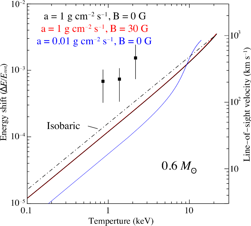
Figure 2: $\Delta E/E_{\rm rest}$ and the line-of-sight plasma velocity measured with the emission lines of H-like Mg, Si, and S ions (squares). The temperature of data points represents the line peak emissivity temperature of the the corresponding ion (see the text). Each error bar shows the sum of the statistical error for a $90$% confidence and the instrumental absolute energy uncertainty. The lines represent theoretical temperature-velocity relations (Hayashi & Ishida, 2014) of the plasma flow with the WD mass of $0.6$ $M_{\odot}$ assuming the exact pole-on geometry: thick solid lines are the cases of $a$ = 1 g cm^-2 cm^-1 and $B$ = 0 G (black), $a$ = 1 g cm^-2 cm^-1 and $B$ = 30M G (red), and $a$ = 0.01 g cm^-2 cm^-1 and $B$ = 0 G (blue). The black dash-dotted line shows the isobaric accretion flow.

We investigated other possibilities that increase the $\Delta E/E_{\rm rest}$. RX J1712.6$-$2414 is located at ($l$, $b$) = ($+359^{\circ}\!\!.87$, $+8^{\circ}\!\!.74$) in the Galactic coordinate, and its distance and proper motions ($\mu_{\rm ra}$, $\mu_{\rm dec}$) are 699.7${}_{-10.8}^{+9.7}$ pc and (-1.765, 2.557) in mas yr^-1 (Gaia Collaboration et al., 2022; Bailer-Jones et al., 2021), respectively. Assuming the space motion along the galactic pole $W=0$, the radial velocity is calculated at $-$2 km s^-1. Indeed, the optical spectra obtained from the South African Astronomical Observatory revealed that the systemic velocity is less than $20$ km s^-1(Buckley et al., 1995). Furthermore, the line-of-sight velocity associated with the binary motion is nullified in our phase-averaged spectra and does not affect the result.

Although significant optical depth shifts the energy centroids of the emission lines (Del Zanna et al., 2002), it is not enough to explain the observed redshifts. The K_α lines are ensembles of the K_α2 and K_α1 lines, whose intensity ratio ($I_{{\rm K}_{\alpha 2}}/I_{{\rm K}_{\alpha 1}}$) affects the energy centroid of the K_α lines. The optical depth at the K_α1 line is double that at the K_α2 line. Therefore, the K_α1 line is more easily attenuated than the K_α2 line; thus, the K_α line energy centroid shifts toward the red side. This effect approximately halves $I_{{\rm K}_{\alpha 1}}/I_{{\rm K}_{\alpha 2}}$ and makes it unity at the optically thick limit (Kastner & Kastner, 1990; Mathioudakis et al., 1999) (see Appendix). We fitted the power-law and 2-Gaussians model in the same manner in $\S$3 by assuming $I_{{\rm K}_{\alpha 1}}/I_{{\rm K}_{\alpha 2}}=1$. The computed $\Delta E/E_{\rm rest}$ and velocity are also presented in Table 2, which still shows the velocities of $\raisebox{-2.15277pt}{$\>\stackrel{{\scriptstyle\textstyle>}}{{\sim}}\>$}1\times 10^{2}$ km s^-1. Although all of them are consistent with the corresponding result with $I_{{\rm K}_{\alpha 1}}/I_{{\rm K}_{\alpha 2}}=2$ within the statistical error, the H-like Si K_α line gave us the best-fit $\Delta E/E_{\rm rest}$, different from the corresponding by $4\times 10^{-4}$. However, this line showed a fine structure in the fitting residual (see Figure 5), implying that optically thick limit (i.e., $I_{{\rm K}_{\alpha 2}}/I_{{\rm K}_{\alpha 1}}=1$) is not a good assumption.

The H-like K_α lines from the pre-shock accreting gas do not contaminate those lines from the post-shock plasma. The pre-shock accreting plasma close to the shock is photoionized by the X-ray irradiation from the post-shock plasma and emits H-like K_α lines (Luna et al., 2010). However, the velocity of the pre-shock gas is 4.1$\times 10^{3}$ km s^-1 and $\Delta E/E_{\rm rest}$ = 1.4$\times 10^{-2}$ with the pole-on geometry even if the WD is light as much as possible i.e., 0.6 $M_{\odot}$. Such highly Doppler-shifted line spectroscopically goes out of the line of the same ion from the post-shock plasma.

Consequently, we conclude that the measured $\Delta E/E_{\rm rest}$ requires a gravitational redshift caused by the WD. Considering the gravitational redshift to our accretion-flow model (Hayashi & Ishida, 2014), as well as the systemic velocity and the instrumental absolute energy accuracy, we estimated the WD mass of RX J1712.6$-$2414 to be $>0.9$ $M_{\odot}$ (Figure 3). The WD mass estimated by previous works (e.g., $0.62^{+0.06}_{-0.05}\,M_{\odot}$(Yuasa et al., 2010), $0.72\pm 0.05\,M_{\odot}$(Suleimanov et al., 2019), and $0.67^{+0.06}_{-0.05}\,M_{\odot}$(Shaw et al., 2020)) is lighter than ours. One plausible explanation for the discrepancy is the cyclotron cooling that softens the X-ray spectrum and was not considered in the previous mass estimations. The magnetic field of RX J1712.6$-$2414 is $(9-27)\times 10^{6}$ G and comparable to that of polars in which the cyclotron cooling is significant (Wu et al., 1994). Another reasonable reason is the X-ray reflection that is maximized at the pole-on geometry and causes complicated systematic error (Hayashi et al., 2021). In previous studies, X-ray reflection was not taken into account.

Lastly, we note that more precise spectral modeling reduces the contribution of the plasma velocity to the redshift, which improves the accuracy of the gravitational redshift estimation. We assume that the H-like K_α lines are emitted at the corresponding line peak emissivity temperature. However, the lines are indeed emitted from a temperature range specified for each ion. Accreting plasma neighboring on the WD has higher density and thus emits more intense X-rays. Meanwhile, the neighboring plasma is slower so that the velocity average weighted over the X-ray intensity is slower than the velocity at the line peak emissivity temperature we used in Figures 2 and 3. The more precise spectral modeling may necessitate greater WD mass, but it is beyond our main aim to report the gravitational redshift detection.

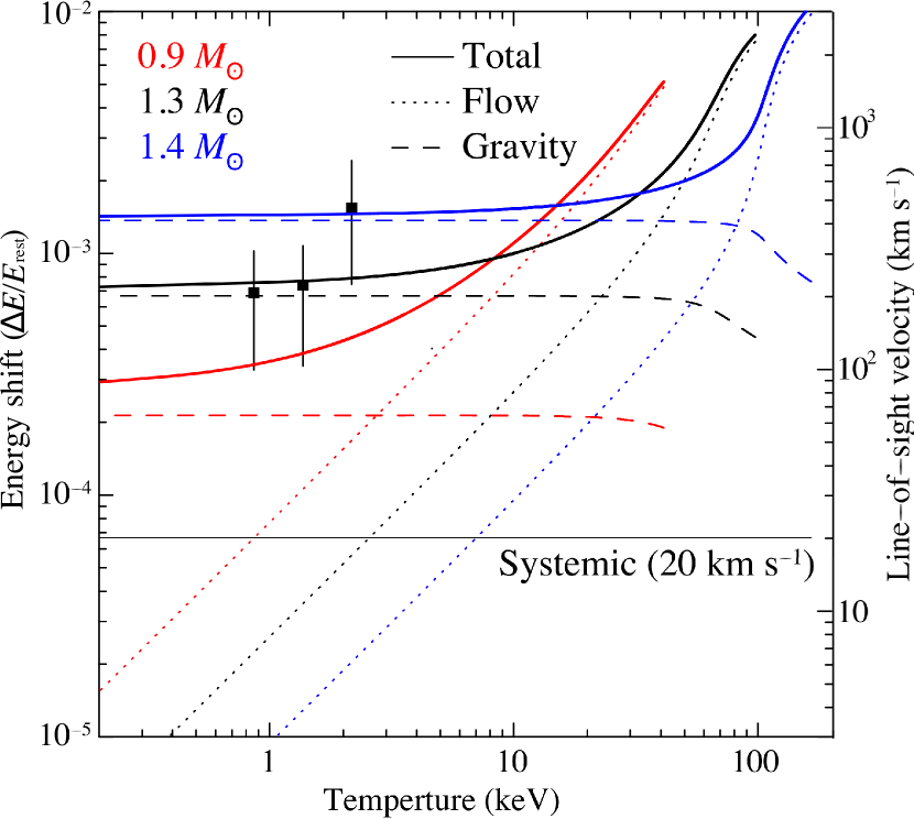
Figure 3: Same as Figure 2, except for theoretical calculations involving the binary system motion and the gravitational redshift. Thick solid lines represent the calculations with the WD mass of $0.9\,M_{\odot}$ (red), $1.3\,M_{\odot}$ (black), and $1.4\,M_{\odot}$ (blue). The dashes, dotted, and thin lines show the components of the gravitational redshift, the plasma flow velocity (Hayashi & Ishida, 2014), and the binary systemic velocity, respectively. The pole-on geometry is assumed for the calculations.

5 Conclusion

We observed the diskless intermediate polar RX J1712.6-2414 with the High-Energy Transmission Grating (HETG) of the Chandra Observatory to study the velocity profile of the plasma in the accretion flow. We found significant redshifts for the K$\alpha$ lines of hydrogen-like magnesium, silicon ($\Delta E/E_{\rm rest}\sim 7\times 10^{-4}$), and sulfur ($\Delta E/E_{\rm rest}\sim 15\times 10^{-4}$) ions, which are above the instrumental absolute energy accuracy (${\Delta E/E_{\rm rest}\sim 3.3}\times 10^{-4}$). We considered several factors producing the redshift, such as the Doppler shift associated with the plasma flow velocity and the systemic velocity, the optical depth, and the gravitational redshift, and then concluded that the gravitational redshift is the major contributor to the observed redshift. This is the first gravitational redshift detection from a magnetic WD. The gravitational redshift provides us with a new method of the WD mass measurement, which estimates the WD mass to be $M_{\rm WD}>0.9\,M_{\odot}$.

Plasma flow model

An accretion plasma flow channelled by a magnetic field is modeled as a 1-dimensional flow. Fundamental equations of a 1-dimensional flow are the mass continuity equation:

$$\frac{{\rm d}}{{\rm d}z}(\rho v)=0,$$ (1)

the momentum equation:

$$\rho v\frac{{\rm d}v}{{\rm d}z}+\frac{{\rm d}P}{{\rm d}z}=\rho F,$$ (2)

and the energy equation:

$$\frac{\rm d}{{\rm d}z}\left[v\left(\frac{1}{2}\rho v^{2}+\frac{\gamma P}{\gamma-1}\right)\right]=\rho vF-\varepsilon.$$ (3)

Here, $\rho$ denotes mass density, $v$ presents flow velocity, $P$ denotes pressure, $F$ is an external force, $\epsilon$ is a radiative cooling rate, and $\gamma$ is an adiabatic index of $5/3$. The integral form of equation 1 is

$$\rho v=a,$$ (4)

where $a$ is called a specific accretion rate, that is, the accretion rate per unit area. The simultaneous equations 2, 3 and 4 are resolved under initial conditions derived from the strong-shock jump condition calculated by the Rankine-Hugoniot relations with the free-fall velocity:

$$v_{0} = 0.25\sqrt{2GM_{\rm WD}/(R_{\rm WD}+h)},$$ (5)

$$\rho_{0} = \frac{a}{v_{0}},$$ (6)

$$P_{0} = 3av_{0},$$ (7)

$$T_{0} = 3\frac{\mu m_{\rm H}}{k}v_{0}^{2},$$ (8)

where $M_{\rm WD}$ is a WD mass, $R_{\rm WD}$ is a WD radius, $G$ is the constant of gravitation, and $h$ is a shock height. The equation of state for the ideal gas is used:

$$P=\frac{\rho kT}{\mu m_{\rm H}}.$$ (9)

A boundary condition of soft landing is also assumed at the WD surface:

$$v_{\rm WD}=0.$$ (10)

By assuming that the shock height is negligibly low compared with the WD radius ($R_{\rm WD}\gg h$, i.e., the post-shock region is low enough), the Bernoulli’s principle requires the total of the pressure and the ram pressure is constant:

$$P_{0}+\rho_{0}v_{0}^{2}=P_{\rm WD}={\rm constant},$$ (11)

where $P_{\rm WD}$ is the pressure at the WD surface at which the velocity is zero. From equations 4 and 7, we obtain

$$P_{0}=3\rho_{0}v_{0}^{2}.$$ (12)

In other words, the pressure is increased only by a factor of 4/3 through the entire flow. Thus, an isobaric flow is a good approximation. With the constant pressure, from equations 4 and 9, the following is derived:

$$\frac{v}{v_{0}}=\frac{\rho_{0}}{\rho}=\frac{T}{T_{0}}.$$ (13)

From equations 5, 8 and 13, the relation between the temperature and the velocity is written as

$$v=\frac{v_{0}}{T_{0}}T=\left(\frac{3\mu m_{\rm H}}{4k}\sqrt{\frac{2GM_{\rm WD}}{R_{\rm WD}}}\right)^{-1}T.$$ (14)

A result of this simple analytical model is shown in the dot-dash line (labelled with “isobaric”) in Figures  2 and 3.

Assuming only the Bremsstrahlung for the radiation cooling process, equations 2, 3, 4, and 13 give us a simple thermal function of $z$:

$$\frac{T}{T_{0}}=\left(\frac{z}{h}\right)^{2/5},$$ (15)

where

$$h=kT_{0}^{1/2}v_{0}/({\mu m_{\rm H}}\Lambda_{\rm m,br}\rho_{0})$$ (16)

and

$$\Lambda_{\rm m,br}\sim 7\times 10^{20}\,{\rm erg\,g^{-1}\,s^{-1}}.$$ (17)

More realistic models have been numerically calculated. The cooling via line emission is included into the cooling function according to plasma codes (Yuasa et al., 2010; Hayashi & Ishida, 2014). Some models involve the cyclotron cooling, which is usually important in the polars (this radiation mainly appears in the infrared band), as well by assuming optically thick radiation (Wada et al., 1980; Cropper et al., 1999; Belloni et al., 2021). Note that the difference in the cooling function does not affect the relation between the temperature and velocity, as shown in equation 14. Moreover, in a real plasma flow with finite height, the gravitational force works. $F$ in equations 2 and 3 is represented as follows to include this effect.

$$F=\frac{GM_{\rm WD}}{(R_{\rm WD}+z)^{2}}.$$ (18)

The calculation of the realistic model are shown in Figures  2 and 3.

Optical depth

The observed intensity ratio of K_α1 and K_α2 is represented by

$$\frac{I_{{\rm K}_{\alpha 1}}}{I_{{\rm K}_{\alpha 2}}}=\frac{I_{{\rm 0,K}_{\alpha 1}}}{I_{{\rm 0,K}_{\alpha 2}}}\frac{p_{{\rm K}_{\alpha 1}}}{p_{{\rm K}_{\alpha 2}}}=2\frac{p_{{\rm K}_{\alpha 1}}}{p_{{\rm K}_{\alpha 2}}}$$ (19)

where $I_{0}$ is the nominal intensity, that is, the intensity at the moment of emission, and $p$ is the probability that an X-ray photon escapes out from the post-shock plasma. The optical depth ($\tau$) at the central energy of a line is proportional to the oscillator strength ($f$) of the corresponding transition (Jordan, 1978). Moreover, the oscillator strength of a K_α1 line is double that of the K_α2 line as

$$\frac{\tau_{{\rm K}_{\alpha 1}}}{\tau_{{\rm K}_{\alpha 2}}}=\frac{f_{{\rm K}_{\alpha 1}}}{f_{{\rm K}_{\alpha 2}}}=2.$$ (20)

The ratio of the escape probability was calculated (Kastner & Kastner, 1990) for a situation in which the emitters (i.e., excited H-like ions) and absorbers (i.e., H-like ions at the ground state) are identically distributed as in the post-shock plasma. Figure 4 depicts the escape probability ratio for lines with an optical depth ratio of 2, i.e., K_α1 and K_α2. At the optically thick limit, the escape probability ratio approximately converges on 0.5 and $I_{{\rm K}_{\alpha 1}}/I_{{\rm K}_{\alpha 2}}\simeq 1$ at the optically thick limit from equation 19.

Figure 4: The ratio of the escape probability of K${}_{\alpha}1$ line to K${}_{\alpha}2$ line as a function of optical depth of the K${}_{\alpha}1$ line (log$\tau_{\rm K_{\alpha 1}}$).

We fitted the power-law and 2-Gaussians model for Mg, Si, and S in the same manner in the $\S$3 by using $I_{{\rm K}_{\alpha 1}}/I_{{\rm K}_{\alpha 2}}=1$. Figure 5 shows the best-fit models with the data and Table 2 shows the best-fit energy shift and velocity.

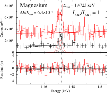
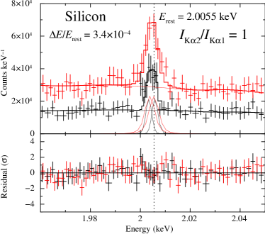
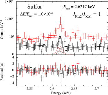
Figure 5: Same as the spectra of Mg, Si, and S in Figure 1, except for the optically-thick limit assumption ($I_{{\rm K}_{\alpha 1}}/I_{{\rm K}_{\alpha 2}}$ = 1 for H-like ion K_α lines).

References

- Aizu (1973) Aizu, K. 1973, Progress of Theoretical Physics, 50, 344, doi: 10.1143/PTP.50.344
- Arnaud (1996) Arnaud, K. A. 1996, in Astronomical Society of the Pacific Conference Series, Vol. 101, Astronomical Data Analysis Software and Systems V, ed. G. H. Jacoby & J. Barnes, 17
- Bailer-Jones et al. (2021) Bailer-Jones, C. A. L., Rybizki, J., Fouesneau, M., Demleitner, M., & Andrae, R. 2021, AJ, 161, 147, doi: 10.3847/1538-3881/abd806
- Belloni et al. (2021) Belloni, D., Rodrigues, C. V., Schreiber, M. R., et al. 2021, Astrophysical Journal Supplement Series, 256, 45, doi: 10.3847/1538-4365/ac141c
- Buckley et al. (1995) Buckley, D. A. H., Sekiguchi, K., Motch, C., et al. 1995, Monthly Notices of the Royal Astronomical Society, 275, 1028, doi: 10.1093/mnras/275.4.1028
- Chandrasekhar (1931) Chandrasekhar, S. 1931, Astrophysical Journal, 74, 81, doi: 10.1086/143324
- Claver et al. (2001) Claver, C. F., Liebert, J., Bergeron, P., & Koester, D. 2001, ApJ, 563, 987, doi: 10.1086/323792
- Cropper (1990) Cropper, M. 1990, Space Science Reviews, 54, 195, doi: 10.1007/BF00177799
- Cropper et al. (1999) Cropper, M., Wu, K., Ramsay, G., & Kocabiyik, A. 1999, Monthly Notices of the Royal Astronomical Society, 306, 684, doi: 10.1046/j.1365-8711.1999.02570.x
- Das et al. (2013) Das, U., Mukhopadhyay, B., & Rao, A. R. 2013, Astrophysical Journal, Letters, 767, L14, doi: 10.1088/2041-8205/767/1/L14
- Del Zanna et al. (2002) Del Zanna, G., Landini, M., & Mason, H. E. 2002, Astronomy and Astrophysics, 385, 968, doi: 10.1051/0004-6361:20020164
- Einstein (1916) Einstein, A. 1916, Annalen der Physik, 354, 769, doi: 10.1002/andp.19163540702
- Frank et al. (2002) Frank, J., King, A., & Raine, D. J. 2002, Accretion Power in Astrophysics: Third Edition
- Fruscione et al. (2006) Fruscione, A., McDowell, J. C., Allen, G. E., et al. 2006, in Society of Photo-Optical Instrumentation Engineers (SPIE) Conference Series, Vol. 6270, Society of Photo-Optical Instrumentation Engineers (SPIE) Conference Series, ed. D. R. Silva & R. E. Doxsey, 62701V, doi: 10.1117/12.671760
- Gaia Collaboration et al. (2022) Gaia Collaboration, Vallenari, A., Brown, A.G.A., Prusti, T., & et al. 2022, A&A, doi: 10.1051/0004-6361/202243940
- Greenstein & Trimble (1967) Greenstein, J. L., & Trimble, V. L. 1967, ApJ, 149, 283, doi: 10.1086/149254
- Hayashi & Ishida (2014) Hayashi, T., & Ishida, M. 2014, Monthly Notices of the Royal Astronomical Society, 438, 2267, doi: 10.1093/mnras/stt2342
- Hayashi et al. (2021) Hayashi, T., Kitaguchi, T., & Ishida, M. 2021, Monthly Notices of the Royal Astronomical Society, 504, 3651, doi: 10.1093/mnras/stab809
- Ishibashi et al. (2006) Ishibashi, K., Dewey, D., Huenemoerder, D. P., & Testa, P. 2006, Astrophysical Journal, Letters, 644, L117, doi: 10.1086/505702
- Jordan (1978) Jordan, C. 1978, in Progress in Atomic Spectroscopy, part A, ed. W. Hanle & H. Kleinpoppen, 1453
- Joshi et al. (2019) Joshi, A., Pandey, J. C., & Singh, H. P. 2019, The Astronomical Journal, 158, 11, doi: 10.3847/1538-3881/ab1ea6
- Joyce et al. (2018) Joyce, S. R. G., Barstow, M. A., Holberg, J. B., et al. 2018, Monthly Notices of the Royal Astronomical Society, 481, 2361, doi: 10.1093/mnras/sty2404
- Kastner & Kastner (1990) Kastner, S. O., & Kastner, R. E. 1990, Journal of Quantitiative Spectroscopy and Radiative Transfer, 44, 275, doi: 10.1016/0022-4073(90)90033-3
- Koester (1987) Koester, D. 1987, ApJ, 322, 852, doi: 10.1086/165779
- Long & Gilliland (1999) Long, K. S., & Gilliland, R. L. 1999, Astrophysical Journal, 511, 916, doi: 10.1086/306721
- Luna et al. (2010) Luna, G. J. M., Raymond, J. C., Brickhouse, N. S., et al. 2010, Astrophysical Journal, 711, 1333, doi: 10.1088/0004-637X/711/2/1333
- Mathioudakis et al. (1999) Mathioudakis, M., McKenny, J., Keenan, F. P., Williams, D. R., & Phillips, K. J. H. 1999, Astronomy and Astrophysics, 351, L23
- Mukai (2017) Mukai, K. 2017, Publications of the Astronomical Society of the Pacific, 129, 062001, doi: 10.1088/1538-3873/aa6736
- Parsons et al. (2012) Parsons, S. G., Marsh, T. R., Gänsicke, B. T., et al. 2012, Monthly Notices of the Royal Astronomical Society, 420, 3281, doi: 10.1111/j.1365-2966.2011.20251.x
- Parsons et al. (2017) Parsons, S. G., Gänsicke, B. T., Marsh, T. R., et al. 2017, Monthly Notices of the RAS, 470, 4473, doi: 10.1093/mnras/stx1522
- Pasquini et al. (2019) Pasquini, L., Pala, A. F., Ludwig, H. G., et al. 2019, Astronomy and Astrophysics, 627, L8, doi: 10.1051/0004-6361/201935835
- Patterson (1994) Patterson, J. 1994, Publications of the ASP, 106, 209, doi: 10.1086/133375
- Perlmutter et al. (1999) Perlmutter, S., Aldering, G., Goldhaber, G., et al. 1999, Astrophysical Journal, 517, 565, doi: 10.1086/307221
- Riess et al. (1998) Riess, A. G., Filippenko, A. V., Challis, P., et al. 1998, Astronomical Journal, 116, 1009, doi: 10.1086/300499
- Shaw et al. (2020) Shaw, A. W., Heinke, C. O., Mukai, K., et al. 2020, Monthly Notices of the Royal Astronomical Society, 498, 3457, doi: 10.1093/mnras/staa2592
- Silvestri et al. (2001) Silvestri, N. M., Oswalt, T. D., Wood, M. A., et al. 2001, AJ, 121, 503, doi: 10.1086/318005
- Sion et al. (1998) Sion, E. M., Cheng, F. H., Szkody, P., et al. 1998, Astrophysical Journal, 496, 449, doi: 10.1086/305378
- Smith et al. (2006) Smith, A. J., Haswell, C. A., & Hynes, R. I. 2006, Monthly Notices of the Royal Astronomical Society, 369, 1537, doi: 10.1111/j.1365-2966.2006.10409.x
- Steeghs et al. (2007) Steeghs, D., Howell, S. B., Knigge, C., et al. 2007, Astrophysical Journal, 667, 442, doi: 10.1086/520702
- Suleimanov et al. (2019) Suleimanov, V. F., Doroshenko, V., & Werner, K. 2019, Monthly Notices of the Royal Astronomical Society, 482, 3622, doi: 10.1093/mnras/sty2952
- van Spaandonk et al. (2010) van Spaandonk, L., Steeghs, D., Marsh, T. R., & Parsons, S. G. 2010, Astrophysical Journal, Letters, 715, L109, doi: 10.1088/2041-8205/715/2/L109
- Wada et al. (1980) Wada, T., Shimizu, A., Suzuki, M., Kato, M., & Hoshi, R. 1980, Progress of Theoretical Physics, 64, 1986, doi: 10.1143/PTP.64.1986
- Wegner et al. (1989) Wegner, G., Reid, I. N., & McMahan, R. K. 1989, in IAU Colloq. 114: White Dwarfs, ed. G. Wegner, Vol. 328, 378, doi: 10.1007/3-540-51031-1_352
- Wu et al. (1994) Wu, K., Chanmugam, G., & Shaviv, G. 1994, Astrophysical Journal, 426, 664, doi: 10.1086/174103
- Xu et al. (2016) Xu, X.-j., Wang, Q. D., & Li, X.-D. 2016, Astrophysical Journal, 818, 136, doi: 10.3847/0004-637X/818/2/136
- Yuasa et al. (2010) Yuasa, T., Nakazawa, K., Makishima, K., et al. 2010, Astronomy and Astrophysics, 520, A25, doi: 10.1051/0004-6361/201014542