The muphyII Code: Multiphysics Plasma Simulation on Large HPC Systems

Abstract

Collisionless astrophysical and space plasmas cover regions that typically display a separation of scales that exceeds any code’s capabilities. To help address this problem, the muphyII code utilizes a hierarchy of models with different inherent scales, unified in an adaptive framework that allows stand-alone use of models as well as a model-based dynamic and adaptive domain decomposition. This requires ensuring excellent conservation properties, careful treatment of inner-domain model boundaries for interface coupling, and robust time-stepping algorithms, especially with the use of electron subcycling. This multi-physics approach is implemented in the muphyII code, tested on different scenarios of space plasma magnetic reconnection, and evaluated against space probe data and higher-fidelity simulation results from literature. Adaptive model refinement is highlighted in particular, and a hybrid model with kinetic ions, pressure-tensor fluid electrons, and Maxwell fields is appraised.

1 Introduction

In collisionless astrophysical and space plasmas, small-scale kinetic effects can have a significant impact on global dynamics. A widely known example is magnetic reconnection, where global quantities such as reconnection time, energy release, and outflow velocities are determined by kinetic effects associated with a highly non-Gaussian velocity distribution function. On the other hand, the large-scale structures thus altered will affect the geometry of the current sheet and, therefore, the reconnection scenario. Numerical modeling of this coupling of kinetic and global scales is a major challenge in global simulations of astrophysical and space plasmas. Due to the vast separation of scales, very few global kinetic simulations exist that model the entire plasma region with numerical schemes based on the Vlasov equation (e.g. [1]) or a hybrid electron fluid/ion Vlasov approach (e.g. [2]). Scales may range, for example, from the electron inertial length to global scales, such as the distance of the magnetotail reconnection region to Earth’s bow shock.

Thus, a dynamic multiphysics approach could be the desired strategy. In this paper, we present such an approach (implemented in the muphyII code) where a hierarchy of models, ranging from full kinetic Vlasov simulations to five-/ten-moment two-fluid models, is coupled in a model-adaptive way. This enables us to perform ”intermediate scale” simulations ranging from the electron scales up to several hundreds of ion inertial lengths. An asymptotic preserving coupling [3] to the magnetohydrodynamic equations (MHD) is also envisioned, which will allow for truly global simulations.

Multiphysics techniques and the idea of coupling different physical models are not new and have been applied in different physical contexts. Schulze et al. [4] couple kinetic Monte-Carlo and continuum models in the context of epitaxial growth. Substantial efforts have been undertaken to couple kinetic Boltzmann descriptions to fluid models (see e.g. [5, 6, 7, 8, 9, 10, 11]. Kolobov and Arslanbekov [12] described the transition from neutral gas models to models of weakly ionized plasmas.

In the context of space plasma physics, Sugiyama and Kusano [13] have begun coupling MHD and particle-in-cell (PIC) models and tested this approach on a 1D Alfvén wave test problem where the MHD and PIC regions were fixed in advance. Markidis et al. [14] introduce a bulk coupling of a four-moment two-fluid/Maxwell solver with an embedded PIC code. The PIC code is used to calculate the closure for the stress and pressure tensors. To achieve the large time steps compatible with the MHD description, an implicit Maxwell solver is used. Daldorff et al. [15] introduced interface coupling to combine kinetic PIC simulations (using the semi-implicit iPIC3D code) with Hall MHD fluid codes (using the BATS-R-US framework). A closely related approach is presented in [16] using MPI-AMRVAC as the MHD solver.

This strategy was applied to global simulations of the magnetotail [17], with the crucial modification of only one-way coupling of the MHD with the PIC solver. The feedback effect of the PIC simulation on the MHD fluid quantities was neglected.

Two-way and adaptive coupling strategies with applications to Magnetosphere simulations were presented in [18, 19, 20]. A recent summary of kinetic modeling/MHD modeling of the magnetosphere can be found in [21]. Also worth mentioning is the multi-level, multi-domain method for Particle-In-Cell simulations [22], which bypasses the reshaping of weight functions in adaptive PIC simulations. Implicit time integration is important in these treatments, such that fast waves, e.g. light, Langmuir, Whistler, and electron drift waves, are damped. Following this approach, an asymptotic preserving scheme to the quasineutral could be achieved as described in [3].

Concerning the coupling to the large-scale MHD equations, Ho, Datta, and Shumlak [23] presented a detailed study and numerical tests on the coupling of the five-moment fluid/Maxwell and the MHD model. They discuss the issue of interface fluxes in the transition from the MHD to the two-fluid model. The difficulty lies in the lack of information on electron quantities. Two approaches have been presented to obtain this missing information. The first leads to conservative fluxes, while the second is physically consistent with the MHD assumptions. The interesting observation was that conservative coupling leads to oscillations, while physically consistent but not conservative coupling leads to a stable scheme.

Another strategy aimed at global simulation is to combine PIC or hybrid simulations with adaptive mesh refinement (see e.g. [24], [25]).

The development of the multi-physics plasma code muphy started with the implementation of a semi-Lagrangian Vlasov code [26]. For the Lagrangian treatment, we developed the backsubstitution method [27] in accordance with Darwin’s approach to Maxwell’s equation to avoid the propagation of light waves [28].

The first version of the muphy framework was presented in [29]. It allowed a static coupling of a kinetic Vlasov code with a two fluid/five-moment model. It utilized distributed MPI/CUDA programming to run on our local cluster of 64 Tesla S1070 GPUs.

In the next development step [30], we aimed at dynamic adaptive coupling of different models (e.g. five-moment, ten-moment, kinetic Vlasov description) where the choice of the model depends on physically motivated model-refinement criteria. This implementation served as a prototype implementation that was not optimized for production runs.

The current version of muphy presented in this paper, muphyII, is a complete rewrite of the prototype implementation aimed at high performance on the JUWELS Booster GPU cluster at the Forschungszentrum Jülich [31]. In addition, it contains a new strategy to conserve energy in the Vlasov simulations as well as subcycling methods for the fast electron dynamics and Maxwell’s equations.

muphyII has already been used extensively in studies of two-fluid simulations of three-dimensional reconnection to understand the role of the lower-hybrid drift instability [32]. In [33] we introduced an energy-conserving Vlasov solver. The bulk coupling to the ten-moment/two-fluid equations allows the choice of coarse velocity resolutions. The resulting scheme was used to study MMS reconnection events. In [34], we implemented a Lagrangian Vlasov solver where the velocity space was approximated by a low-rank hierarchical Tucker decomposition. The low-rank scheme was able to reduce the number of degrees of freedom by almost two orders of magnitude.

2 Physical Models

In muphyII, collisionless models with different levels of physical accuracy and computational cost are implemented. The exact kinetic model for collisionless plasmas, which takes the complete velocity space information into account, describes the plasma using a distribution function $f_{s}(\mathbf{x},\mathbf{v},t)$ for each particle species $s$. The evolution of the distribution function in position space $\mathbf{x}$, velocity space $\mathbf{v}$ and time $t$ is given by the Vlasov equation

$$\frac{\partial f_{s}}{\partial t}+\mathbf{v}\cdot\nabla_{x}f_{s}+\frac{q_{s}}{m_{s}}(\mathbf{E+v\times B})\cdot\nabla_{v}f_{s}=0,$$ (1)

which depends on the electric field $\mathbf{E}$, magnetic field $\mathbf{B}$, and particle species charge and mass, $q_{s}$ and $m_{s}$. We will refer to (1) as Vlasov model.

Integrating over velocity space and truncating the hierarchy after the pressure equation yields a reduced set of equations for particle density $n_{s}=\int f_{S}(\mathbf{x},\mathbf{v},t)\textup{d}\mathbf{v}$, mean velocity $\mathbf{u}_{s}=\nicefrac{{1}}{{n_{s}}}\int\mathbf{v}f_{s}(\mathbf{x},\mathbf{v},t)\textup{d}\mathbf{v}$, and momentum flux density $\mathcal{P}_{s}=m_{s}\int\mathbf{v}\mathbf{v}f_{s}(\mathbf{x},\mathbf{v},t)\textup{d}\mathbf{v}$. They constitute the ten-moment multi-fluid equations,

$$\frac{\partial n_{s}}{\partial t}+\nabla\cdot(n_{s}\mathbf{u}_{s})=0,$$ (2)

$$m_{s}\frac{\partial(n_{s}\mathbf{u}_{s})}{\partial t}-n_{s}q_{s}(\mathbf{E}+\mathbf{u}_{s}\times\mathbf{B})+\nabla\cdot\mathcal{P}_{s}=0,$$ (3)

$$\frac{\partial\mathcal{P}_{s}}{\partial t}-q_{s}(n_{s}\text{sym}(\mathbf{u}_{s}\mathbf{E})+\frac{1}{m_{s}}\text{sym}(\mathcal{P}_{s}\times\mathbf{B}))+\nabla\cdot\mathcal{Q}_{s}=0.$$ (4)

Here, the standard product is the outer (tensor) product, $(\mathbf{a}\mathbf{b})_{ij}=a_{i}b_{j}$, the vector product has been generalized to tensors, $(\mathcal{A}\times\mathbf{b})^{ijk}=\epsilon_{klm}A^{ijl}b^{m}$, and the symmetric operator sums over all cyclic permutations of uncontracted indices, $\mathrm{sym}(\mathcal{A})_{ijk}=A_{ijk}+A_{jki}+A_{kij}$.

We close this set of equations with a Landau-based model for the heat flux $\mathrm{Q}_{s}=\int\mathbf{v}\mathbf{v}\mathbf{v}f_{s}(\mathbf{x},\mathbf{v},t)\textup{d}\mathbf{v}=\mathcal{Q}_{s}-\mathrm{sym}(\mathbf{u}_{s}\mathcal{P}_{s})+2m_{s}n_{s}\mathbf{u}_{s}\mathbf{u}_{s}\mathbf{u}_{s}$ that receives information from the gradient of the temperature $\mathrm{T}_{s}=(\mathcal{P}_{s}-mn\mathbf{u}_{s}\mathbf{u}_{s})/(n_{s}k_{\textup{B}})$, [33, 35, 32]

$$\nabla\cdot\mathrm{Q}_{s}=-\frac{\chi}{k_{s,0}}\,n_{s}\,v_{\textup{th},s}\,\nabla^{2}\,\mathrm{T}_{s}\,,$$ (5)

with thermal velocity $v_{\textup{th},s}=\sqrt{2T_{s}/m_{s}}$ and a free parameter $\chi/k_{s,0}$. We will refer to the set of equations (2,3,4,5) as ten-moment fluid model.

By assuming isotropic pressure and zero heat flux, tensorial pressure reduces to the energy density scalar $\mathcal{E}_{s}=\nicefrac{{m_{s}}}{{2}}\int v^{2}f_{s}(\mathbf{x},\mathbf{v},t)\textup{d}\mathbf{v}$, resulting in a total of five fluid equations,

$$\frac{\partial n_{s}}{\partial t}+\nabla\cdot(n_{s}\mathbf{u}_{s})=0,$$ (6)

$$m_{s}\frac{\partial(n_{s}\mathbf{u}_{s})}{\partial t}-n_{s}q_{s}(\mathbf{E}+\mathbf{u}_{s}\times\mathbf{B})+\frac{1}{N}\nabla(2\mathcal{E}_{s}-m_{s}n_{s}\mathbf{u}_{s}^{2})+\nabla\cdot(m_{s}n_{s}\mathbf{u}_{s}\mathbf{u}_{s})=0,$$ (7)

$$\frac{\partial\mathcal{E}_{s}}{\partial t}-q_{s}n_{s}\mathbf{u}_{s}\cdot\mathbf{E}+\frac{1}{N}\nabla\cdot\Big{(}\mathbf{u}_{s}((N+2)\mathcal{E}_{s}-m_{s}n_{s}u_{s}^{2})\Big{)}=0.$$ (8)

where $N$ is the dimensionality of velocity space. We will refer to the set of equations (6,7,8) as five-moment fluid model.

The evolution of electric and magnetic fields $\mathbf{E}$ and $\mathbf{B}$ is determined by Maxwell’s equations

$$\nabla\cdot\mathbf{E}=\frac{\rho}{\epsilon_{0}}\,,\quad\nabla\cdot\mathbf{B}=0\,,\quad\nabla\times\mathbf{E}=-\frac{\partial\mathbf{B}}{\partial t},\quad\nabla\times\mathbf{B}=\mu_{0}\mathbf{j}+\mu_{0}\varepsilon_{0}\frac{\partial\mathbf{E}}{\partial t}\,$$ (9)

which use charge density $\rho=\sum_{s}q_{s}n_{s}$, current density $\mathbf{j}=\sum_{s}q_{s}n_{s}\mathbf{u}_{s}$, vacuum permittivity $\varepsilon_{0}$, and vacuum permeability $\mu_{0}$. In the electrostatic case, the electric field $\mathbf{E}$ is given by Poisson’s equation

$$\nabla^{2}\Phi=-\frac{\rho}{\epsilon_{0}}$$ (10)

where the electric field is related to the electric potential $\Phi$ through $\mathbf{E}=-\nabla\Phi$.

Currently, muphyII  uses the same mesh spacing for all physical models. The coupling of the five-moment model with our adaptive mesh code racoon  [36] is still in progress.

3 Code Design and Performance

The 2nd-generation multi-physics plasma framework, muphyII, is written in C++ and Fortran, and utilizes the MPI standard for distributed memory parallelism. All solvers are fully three-dimensional and GPU-accelerated using the OpenACC API. The code was designed to prioritize performance, maintainability, and flexibility, and we want to elaborate in this section on the design choices.

C++ was chosen for the framework and logic parts of the code because of its flexibility. For the pure numeric calculations, Fortran was chosen because of the simplicity of its built-in multi-dimensional array operations. This allows for excellent compiler optimization and performance out of the box and makes the numeric implementation easy to write and read at the same time. Good readability and maintainability are very important for a scientific code because (i) it must be easy to check whether a numerical method is implemented correctly, and (ii) the personnel working with the code fluctuates often, especially in university research. In particular, for students who are new to code development and do not only apply the code for physical research but also do research on new numerical methods, a simple code design is crucial. Conveniently, this often also leads to good performance. However, new physical models (like relativistic fluid or kinetic descriptions) can be added in any language like C++ or Julia. They only have to comply with the C++ interface functions.

The distributed memory parallelization utilizes MPI and a classical domain decomposition approach. The physical domain is divided into multiple subdomains (we call them “blocks”), which are each handled by separate computing processes and can handle a different type of the underlying physics (e.g. Vlasov model for ions and ten-moment fluid model for electrons coupled through Maxwell’s equations). The exchange of information between neighboring subdomains is done via MPI and makes use of boundary cells. Inside each subdomain, shared memory parallelization is available and implemented with OpenACC so that GPUs can be utilized. CUDA-aware MPI is supported for fast inter-node communication.

The choice of favoring OpenACC over low-level implementations like CUDA has been made for multiple reasons. The use of OpenACC significantly reduces development time and improves code readability and maintainability. The optimized OpenACC code performs well without rigorous adaption to certain device architectures. Furthermore, it can be run on accelerators from different manufacturers as well as multi-core CPU systems  which makes the muphyII framework very flexible. Finally, the same code base can be used for GPU- and CPU-based supercomputers, again increasing flexibility and maintainability. For good performance on GPUs, it is necessary to manage the GPU data transfers explicitly. Concerning the compute kernels, i.e. operations that are carried out on the GPU, there are two options available in OpenACC: The kernel construct leaves the compiler complete freedom for optimization, whereas the parallel construct gives the developer some possibilities for manual optimization. A very effective optimization strategy that is often used in muphyII is to collapse nested loops over different array dimensions into two loops: One loop that utilizes gang parallelization and one that utilizes vector parallelization, where OpenACC gangs can be compared to CUDA thread blocks and vectors to CUDA threads within the thread block.

The central object in the program layout of muphyII is a block that is associated with an MPI process. Each block holds a “scheme” object that implements the order of numerical solver function calls and boundary exchange calls. The scheme object holds multiple “model” objects which contain the model data (for example the distribution function in a Vlasov equation model or the electromagnetic fields in a Maxwell’s equations model) as well as the implementation of the numerical solvers. An example of a scheme would be a {Vlasov electrons, Vlasov ions, Maxwell} scheme, which has a Vlasov model object for each of the species and a Maxwell model object. The design philosophy where each block/subdomain in the domain decomposition can hold a different physical scheme meshes well with the multiphysics approach of muphyII. Depending on the physical necessity, the subdomains can be treated with different physical models. Simplified UML diagrams summarizing these features are shown in figures 1 and 2.

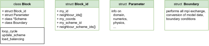
Figure 1: The framework of muphyII, which is responsible for the parallelization, boundary exchanges and conversions, data output and scheme/model adaption is mostly hidden from the user.

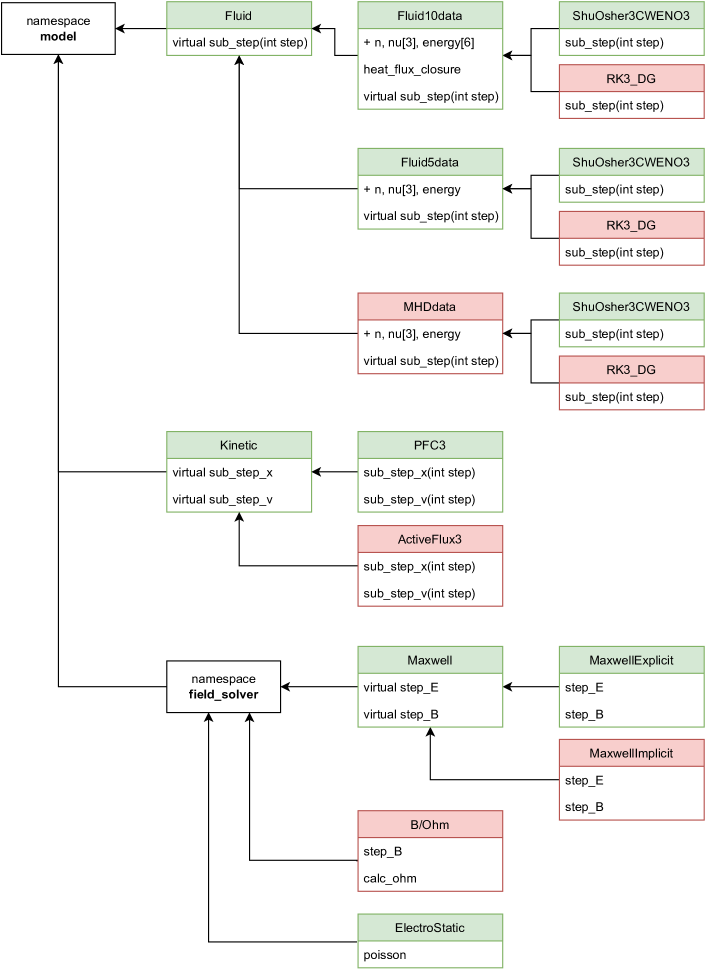
Figure 2: The class Scheme contains all possible combinations of the Model classes. Schemes and models should be easily adjustable and added by the user. Models colored green are stable, whereas the models colored red are work in progress.

In such spatially coupled simulations, the blocks with kinetic models take significantly more computational time than those with fluid models. The difference in computational cost is addressed using the CUDA multi-process service (MPS). There, multiple MPI processes can share a single GPU. The idea is to have one or few kinetic blocks on each GPU, together with a large number of fluid blocks. Then, ideally, the few kinetic blocks use the GPU to full capacity in the first part of the numerical scheme, and the many fluid blocks together also use the GPU to full capacity in the second part of the numerical scheme. Load balancing is implemented such that equally many expensive and less expensive models are computed by each GPU.

Figure 3: Computing time scaling of muphyII on the JUWELS-booster supercomputer. Shown is the weak scaling where the number of cells and the number of GPUs is increased at the same time.

The weak scaling of muphyII on the JUWELS-booster supercomputer [37] is shown in fig. 3. It scales excellently up to 1024 A100 GPUs (more than 7 million GPU cores), and the scaling is expected to continue in the same manner towards higher numbers. The increase in step duration at 64 GPUs is due to the network layout of JUWELS-booster. In JUWELS-booster, network cells consisting of 48 nodes are connected with very high bandwidth, and multiple network cells are connected with slightly lower bandwidth. The increase in step duration is caused by communication over multiple network cells and is unrelated to the implementation. The scaling study was performed in double precision, making use of the matched moment Vlasov method (see sec. 4.1) in the kinetic case and the ten-moment multi-fluid model (see sec. 4.1) with temperature gradient heat flux closure (5) in the fluid case, and using 15 subcycles (see sec. 4.4) of the FDTD Maxwell solver (see sec. 4.1). As a physical setup, we chose an Orszag-Tang vortex for the kinetic solver in 2D3V [38] and for the fluid solver in 3D [39]. The time step duration was averaged over 100 steps after a warm-up phase of 50 steps.

4 Numerical Methods

4.1 Solvers

For the solution of the physical equations given in Sec. 2, different numerical solvers are implemented in muphyII. The Vlasov equation (1) is solved on a phase space grid with a semi-Lagrangian scheme [40] using the positive and flux-conservative (PFC) method [41]. We implement the spatially third-order version and use the limiter only for small values of the phase space distribution function to guarantee positivity. The position space and velocity space updates are performed with leapfrog-like Strang splitting. Formally, the Strang method is only a second-order method with respect to time. However, the special nature of the advection terms in the Vlasov equation leads empirically to a method of higher than second order. As a result, a time order of $2.4$ is usually obtained. We perform further splitting of the advection operator in the three spatial directions and the three velocity space directions, respectively. The splitting in the three spatial directions introduces no additional errors since the advection operators commute. The velocity space splitting is realized via backsubstitution [27]. To conserve total energy and to relax the numerical requirements concerning velocity space resolution, the matched-moments Vlasov solver [33] is utilized (see Algorithm 1 for details).

The ten- and five-moment equations are solved by means of the CWENO finite volume method [42]. Time integration is done with a three-step Runge-Kutta method with good stability properties [43]. Several heat flux closures to the ten-moment equations are implemented: The pressure gradient closure [35, 32], the temperature gradient closure [33], the temperature gradient closure by Ng et al. (2020) [44] and the isotropization closure by Wang et al. (2015) [45]. The gradient closures are subcycled, as they often need a lower time step for stability than the fluid equations themselves. For numerical stability, an explicit floor is set for the pressure.

Maxwell’s equations are solved via the finite difference time domain (FDTD) method. The two Maxwell’s equations that include time derivatives are evolved, and it is, by construction of the method, ensured that $\nabla\cdot\mathbf{B}=0$. Furthermore, Gauss’s law $\nabla\cdot\mathbf{E}=\rho/\epsilon_{0}$ is fulfilled in a vacuum or when the numerical method that provides the current density meets some requirements. For good preservation of Gauss’s law, the current density in the matched-moments Vlasov and fluid schemes is calculated from the CWENO cell fluxes. For electrostatic simulations, a simple iterative Poisson solver is implemented that is parallelized via additive Schwarz iterations.

4.2 Time Stepping Scheme

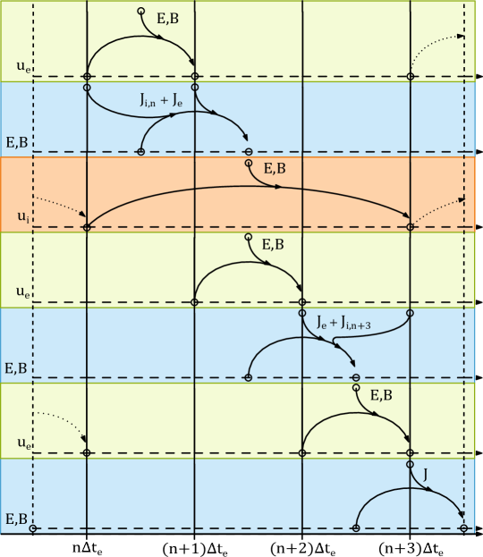
Figure 4: Schematic diagram of the time stepping with electron subcycling for $N_{e}=3$. Operations are executed from top to bottom, and numeric time goes left to right. Advance operations are highlighted with colors based on their context for visual aid (blue: fields solver, green: electron plasma solver, orange: ion plasm

a solver).

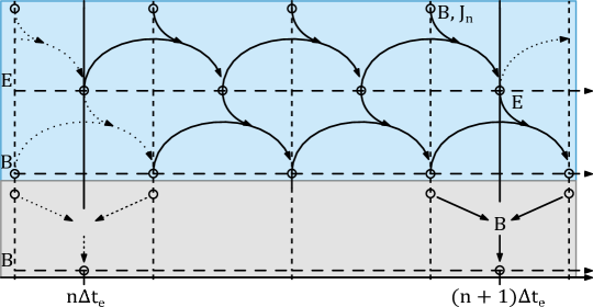
Figure 5: Schematic diagram of the leapfrog-like Maxwell subcycling for $N_{m}=3$. Operations are executed from top to bottom; numeric time goes left to right. Operations are highlighted with colors based on their algorithmic context for visual aid (blue: advance, grey: interpolation).

To take advantage of the different time resolution requirements of Maxwell’s equations and the two particle species’ equations, the models have the option to employ subcycling to use different step sizes for each solver. The much smaller mass of electrons compared to ions typically leads to much faster motion and requires smaller steps, both for fidelity and stability. For non-relativistic particles, the speed of light is usually also much higher, even when using reduced values. To reflect this, the subcycling is arranged into two parts. For every electron step, the Maxwell update is split into $N_{m}$ Maxwell substeps, and every ion step corresponds to $N_{e}$ electron substeps. The electron and Maxwell states are integrated using Strang splitting, which offsets the latter by half the electron time step.

The Runge-Kutta integrator used in the ten and five-moment solvers, and consequently also the ten-moment solver in the moment-matching algorithm, works with Maxwell field data provided at $t+\Delta t_{s}/2$. For the case of no electron subcycling, the offset due to Strang splitting ensures that this data is calculated for the right times. With more than one electron cycle, this is no longer necessarily true for the ion step. Choosing an uneven amount of electron substeps allows computing the ion step without any additional interpolation by rearranging it after the $\lfloor N_{e}/2\rfloor$-th Maxwell step, as seen in Fig. 4. The Maxwell solver itself uses Strang splitting between $\mathbf{E}$ and $\mathbf{B}$ and the linear interpolation used to obtain $\mathbf{B}$ at the full Electron step times only needs to be calculated at the last substep (see Fig. 5).

While $N_{m}$ is manually set as a parameter of the simulation, $N_{e}$ and the step sizes for each solver are chosen based on the current maximum stable step sizes $\Delta t_{e}^{*}\ ,\ \Delta t_{i}^{*}$ to minimize the amount of ion steps: $N_{e}=\lceil\Delta t_{i}^{*}/\Delta t_{e}^{*}\rceil\ ,\ \Delta t_{i}=\Delta t_{i}^{*}$.

The steps of the moment-matching Vlasov solver are largely identical to the original ones described in [33]. However, to improve the fulfillment of Gauss’s law, the density correction is applied to the non-Maxwellian part of the distribution function instead of the fluid moments. Compare Algorithm 1 below and in the original publication.

Initialize with a half step of the Maxwell solver

Time Step 

       Calculate third moment $\mathcal{Q}^{t}$ from $f^{t}$

       Full Vlasov leapfrog step to advance to $f^{t+1}$

       Calculate $\mathcal{Q}^{t+1}$ from $f^{t+1}$

       Interpolate to get $\mathcal{Q}^{t+1/2}$

       Full Runge-Kutta fluid step (input $\mathcal{Q}$ at appropriate times)

       Moment Fitting 

             Calculate moments $n_{\text{V}}$, $\mathbf{u}_{\text{V}}$, $\mathcal{P}_{\text{V}}$ from $f$

             Calculate ten-moment Maxwellian $f_{\text{M,V}}$ from $n_{\text{V}}$, $\mathbf{u}_{\text{V}}$, $\mathcal{P}_{\text{V}}$

             Calculate ten-moment Maxwellian $f_{\text{M,F}}$ from the fluid solver’s moments

             Exchange ten-moment Maxwellians with density correction: $f=(f-f_{\text{M,V}})\,(n_{\text{F}}/n_{\text{V}})+f_{\text{M,F}}$

             Limit $f$

      Full step of the Maxwell solver

      

Algorithm 1 Time stepping of the moment matching Vlasov-Maxwell solver as it is implemented

4.3 Spatial Coupling

The spatial coupling of different plasma models can significantly reduce the computational time needed for a simulation by applying expensive kinetic models only where kinetic effects are assumed to be important. In many scenarios, large parts of the physical domain can appropriately be treated with much cheaper fluid models.

In muphyII, the whole domain is divided into multiple subdomains that can be computed independently (see the parallelization information in Sec. 3). This fits seamlessly with the spatial coupling multiphysics approach. Each subdomain can contain different plasma models, and the model coupling at the subdomain borders is incorporated into the boundary information exchange process.

The regions where certain models are used can be static, or they can be dynamic, i.e. adapt to the problem over the course of the simulation. For the latter case, criteria are defined to decide which models are to be used based on local plasma quantities. A hierarchy of models that are available for coupling is defined. These models are, starting from physically complete towards more and more reduced: full Vlasov $\rightarrow$ hybrid Vlasov ions, ten-moment fluid electrons $\rightarrow$ full ten-moment fluid $\rightarrow$ ten-moment fluid ions, five-moment fluid electrons $\rightarrow$ full five-moment fluid (see figure 6).

Figure 6: Hierarchy of available models (including the enums used in muphyII.

We allow coupling only between neighboring models in this hierarchy to keep the change in physics at the model boundaries as small as possible. This restriction is supposed to improve physical accuracy and lead to smooth coupling borders. In the boundary exchange between different models, the more reduced data is sent to minimize the communication volume. Before or after sending the boundary data via MPI, it is converted into the appropriate model.

There are two possible model conversions in the hierarchy: Between the five and ten-moment fluid models or between the ten-moment fluid and the Vlasov model. We will discuss both scenarios, starting with the former. Computing a reduced model from the information of a more complete model is typically straightforward. Generating five-moment data out of ten-moment data is done by simply taking the trace of the ten-moment model’s pressure tensor, $\operatorname{tr}(\mathrm{P})$, to get the five-moment’s scalar pressure. The other way around is more difficult because there are degrees of freedom – an infinite amount of different pressure tensors can lead to the same scalar pressure. Since in coupled simulations, we typically use the five-moment model only where the assumption of isotropic (scalar) pressure is appropriate, we choose the most simple solution. The ten-moment boundary data is generated out of the five-moment data by prescribing isotropy, i.e. setting $\mathrm{P}=p/d\,\mathrm{I}$, where $\mathrm{P}$ is the pressure tensor, $p$ is the scalar pressure, and $\mathrm{I}$ the identity matrix. An alternative implementation available in muphyII extends the pressure tensor from the ten-moment solution at the coupling border into the boundary cells and multiplies the pressure tensor by a scalar factor such that it matches the scalar pressure provided by the five-moment model.

The other model transition is between the Vlasov and the ten-moment model. Again, it is straightforward to compute the ten-moment data out of the distribution function boundary data provided by the Vlasov model, and again, there are infinite possibilities to construct distribution functions that match the ten-moment boundary data. The first guess is to use a ten-moment Maxwellian distribution, which takes the temperature tensor into account (a multivariate normal distribution), as this is the maximum entropy solution. This approach already leads to good results. For an even smoother transition, we extend the Vlasov data at the coupling border into the boundary cells and adjust it to match the fluid boundary data. This method was introduced in Rieke et al. [29] and Trost et al. [46], however the way of adjusting the distribution function is now done by exchanging Maxwellians [33]. We remove the ten-moment Maxwellian part from the extended Vlasov data and add the result, multiplied by a factor $\sigma_{i}$, to the Maxwellian computed from the fluid boundary data. The factor is chosen to decrease linearly with distance to the coupling border. In our case of two boundary cells, it is $\sigma_{1}=2/3$ and $\sigma_{2}=1/3$ in the first and second boundary cells, respectively.

4.4 Hybrid Ten-Moment-Vlasov Model with Electron Subcycling

The hierarchy of models available in muphyII includes a fully kinetic Vlasov model, fluid models, and a hybrid model. While the former have been discussed in earlier papers (e.g. [33, 32]), the latter was used in a simple version in Lautenbach and Grauer (2018) [30], but was not described in detail. Recently, there have been significant additions such as electron subcycling. The novel hybrid approach that we take, using ten-moment fluid electrons, Vlasov ions, and full Maxwell’s equations, shall be introduced in this section.

Hybrid-kinetic plasma models where the ions are treated kinetically and the electrons are treated as a fluid have seen much success. They have been born out of the observation that the ions are more important for the plasma dynamics in many phenomena while, at the same time, the electrons are dramatically more expensive to model. Thus, in many cases, it is a good strategy to approximate the electrons as a fluid so that the kinetic equations need only be solved on ion time and spatial scales. Traditionally, the electron dynamics and electromagnetic field equations are approximated via a generalized Ohm’s law. Often, electrons are considered to be a massless fluid with equations of state for the pressure, typically in the isothermal limit.

There are hybrid-Vlasov codes that solve the ion Vlasov equation on a phase-space grid, e.g. HVM [47, 48] and Vlasiator [2, 49]. On the other hand, there are hybrid-PIC codes that utilize the particle-in-cell method for the ions, e.g. H3D [50] and CAMELIA [51]. Recently, there have been efforts to include pressure anisotropy into the fluid electron approximation for H3D [52] and HVM (then called HVLF) [53].

Here, we go even further and employ a complete ten-moment fluid model for the electrons and use full Maxwell’s equations without approximation. With the help of the electron subcycling and the Maxwell subcycling discussed in Sec. 4.2 it is still possible to solve the ion Vlasov equation only on ion time scales. From a physical point of view, a large ion time step is justified. Numerically, the ions are easier to handle with respect to their time step because they are not accelerated as strongly, and the numeric time step restrictions are lower. The drastic saving in computational time compared to full Vlasov simulations does not only come from the larger time step. Since the electrons are much more accelerated than the ions, especially towards realistic mass ratios, it is necessary to resolve the large electron velocity space with a high number of cells (mostly due to numerics). In contrast, a significantly lower resolution is sufficient for the slower ions, particularly if the moment matching method is used [33]. These two factors together make the hybrid ten-moment-Vlasov model extremely performant while it still includes the complete ion kinetics, represents electron inertia and light waves self-consistently, and includes the full electron pressure tensor and a Landau damping heat flux approximation. In the past, hybrid-PIC methods were often considered to be more performant than hybrid-Vlasov methods due to the large velocity space resolutions necessary for the Vlasov phase-space grid. However, using the matched-moments Vlasov method, we are able to reduce the ion velocity resolution without loss of fidelity and approach a number of freedoms comparable to those used with PIC kinetic solvers. We still avoid numerical issues of hybrid-PIC methods [54], and discrete particle noise.

5 Benchmark Simulations

In this section, we want to show the features of muphyII that have not yet been discussed in earlier publications, which means those that go beyond the fully kinetic and fully fluid cases. On the one hand, this is the coupling of different plasma models, which – compared to the previous muphy code – greatly benefits from the energy-conserving Vlasov solver and the improved heat flux closure as well as from the technological advancements. On the other hand, we test the physical expressiveness of the hybrid ten-moment-Vlasov model, which benefits from the solver improvements as well, but also from the newly developed electron subcycling approach.

5.1 Static Coupling

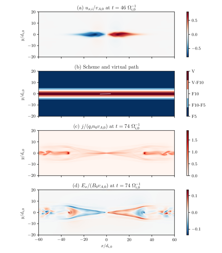
Figure 7: Statically coupled simulation of magnetotail reconnection. (a) Ion outflow velocity, (b) locations where the different numerical schemes are used and the virtual path as a white line, (c) absolute value of the current density, (d) $x$-component of the electric field.

An ideal setup for testing the spatial coupling is given by the magnetotail reconnection event measured by MMS on 11th July 2017 at 22:34 UT [55] with the initial conditions derived in Nakamura et al. (2018) [56] and Genestreti et al. (2018) [57]. This is a good benchmark case firstly because magnetic reconnection is an important yet very complex phenomenon that requires a good representation of kinetic effects. Secondly, for this particular case, spacecraft measurements and highly accurate fully kinetic PIC [56] and Vlasov [33] simulations are available for comparison.

The initial conditions are similar to a Harris equilibrium. The initial particle density is given by ${n_{s}=n_{0}\operatorname{sech}^{2}(y/\lambda)+n_{b}}$ and the magnetic field by ${B_{x}=\tanh(y/\lambda)B_{0}+\delta B_{x}}$, ${B_{y}=\delta B_{y}}$ and ${B_{z}=-B_{g}}$. The background density is ${n_{b}=n_{0}/3}$, the half-thickness of the current sheet ${\lambda=0.6\,d_{i,0}}$ and the guide field ${B_{g}=0.03\,B_{0}}$. The background particles (those related to density $n_{b}$) are initially static and have temperatures ${T_{bg,s}=T_{0,s}/3}$ whereas the sheet particles have temperatures according to ${n_{0}k_{B}(T_{0,e}+T_{0,i})=B_{0}^{2}/(2\mu_{0})}$, ${T_{0,i}/T_{0,e}=3}$ and carry the current. The domain goes from $-L_{x}/2$ to $L_{x}/2$ in $x$-direction and $-L_{y}/2$ to $L_{y}/2$ in $y$-direction where ${L_{x}=120\,d_{i,0}}$ and ${L_{y}=40\,d_{i,0}}$. Here, reconnection is initiated by a small Gaussian perturbation ${\delta B_{x}=-\xi\,(2y/\lambda^{2})\,\exp\left(-(x/(a\lambda))^{2}\right)\exp\left(-(y/\lambda)^{2}\right)B_{0}}$ and ${\delta B_{y}=\xi\,(2x/(a\lambda)^{2})\,\exp\left(-(x/(a\lambda))^{2}\right)\exp\left(-(y/\lambda)^{2}\right)B_{0}}$ where the magnitude of the perturbation is chosen as ${\xi=0.025}$ and ${a=L_{x}/L_{y}}$. Electron velocity space ranges from ${-20\,v_{A,0}}$ to ${20\,v_{A,0}}$ and ion velocity space from ${-5\,v_{A,0}}$ to ${5\,v_{A,0}}$. The ion-electron mass ratio was set to ${m_{i}/m_{e}=100}$ and the speed of light to ${c=20\,v_{A,0}}$. The resolution is ${1536\times 512}$ cells in position space times $36^{3}$ cells in velocity space in the case of the Vlasov models. The ten-moment fluid equations utilize the temperature gradient heat flux closure [33] at 16 subcycles.

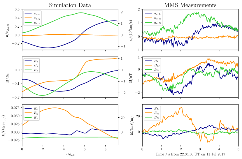
Figure 8: Comparison between MMS measurements (right) and the statically coupled simulation (left). Simulation data was taken along the virtual path shown in Fig. 7 at $t=46\,\Omega_{i,0}^{-1}$.

An overview of the simulation is given in Fig. 7. The structure of the ion outflow velocity (Fig. 7a) matches precisely the one observed in the fully kinetic case (see e.g. the snapshots shown in [57] and [56]). As shown in Fig. 7b, only a very small part of the domain is computed with the fully kinetic model, namely $1/16$, and the largest part is treated with the cheap five-moment fluid model. Nevertheless, important kinetic features are captured. In Fig. 7c, the absolute value of the current density is shown at a later time. The elongated current sheet that is characteristic of kinetic reconnection with small to moderate guide fields [58] is clearly visible together with an instability in the outflow (possibly the firehose instability). To demonstrate the smoothness of the coupling, the $x$-component of the electric field is given in Fig. 7d. This is one of the most sensitive quantities and still shows no signs of irregularities at the coupling borders, although complex features evolve beyond the interfaces between the different models.

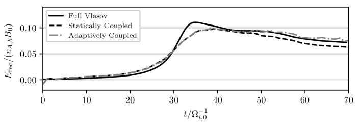
Figure 9: Normalized reconnection rate in the statically and dynamically coupled simulations compared to the full Vlasov simulation from [33] (the latter shifted by $-30\,\Omega_{i,0}^{-1}$ to account for the lower initial perturbation used there).

The coupled simulation compares well to measurements of the MMS spacecraft of the reconnection event, as shown in Fig. 8. The simulation data was taken along the virtual path that is represented by the white line in Fig. 7b. While the agreement between simulation and measurements does not quite reach the quality of fully kinetic simulations [56, 33] (which is expected) it does come close. It is clear that the use of the Vlasov model only in the center of the domain cannot represent all kinetic effects precisely. In [33], the electron heat flux was shown to be the strongest at the separatrix borders, which is absolutely not captured by the five-moment model used there. In the future, a better distribution of the models in the domain could further improve the results. Nevertheless, the result is very encouraging, considering that the kinetic region is so small.

Similar conclusions can be drawn from a comparison of the normalized reconnection rate between the coupled simulation and the fully kinetic Vlasov simulation from [33]. The reconnection rate peaks around the typical value of 0.1 [59] and is overall quite similar between the coupled and the fully kinetic simulation. The coupled result is also comparable to the reconnection rate obtained in [56], which matches the full Vlasov case.

5.2 Dynamic Coupling

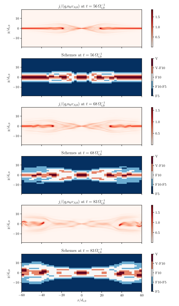
Figure 10: Overview of the dynamically coupled simulation of magnetotail reconnection: Absolute value of the current density and distribution of the different physical schemes at three different times.

Scheme	Description	Criterion
V	Vlasov ions, Vlasov electrons	$j>1.00\ n_{0}v_{A,0}\ \ \lor\ \ u_{e}>4.0\ v_{A,0}$
V-F10	Vlasov ions, 10 mom electrons	$j>0.50\ n_{0}v_{A,0}\ \ \lor\ \ u_{e}>2.0\ v_{A,0}$
F10	10 mom ions, 10 mom electrons	$j>0.20\ n_{0}v_{A,0}\ \ \lor\ \ u_{e}>1.0\ v_{A,0}$
F10-F5	10 mom ions, 5 mom electrons	$j>0.05\ n_{0}v_{A,0}\ \ \lor\ \ u_{e}>0.5\ v_{A,0}$
F5	5 mom ions, 5 mom electrons	else.

Table 1: Criteria used for choosing the plasma models in the dynamically coupled simulation.

Selecting static regions where the different plasma models are used is not the optimal approach in most cases because the areas where certain physical models are required change over time. One example is the electron heat flux at the separatrix borders in the later simulation time. Therefore, we performed a simulation with dynamic coupling where a criterion based on local plasma parameters determines which physical model is used. Here, we choose a heuristic criterion that is tuned for magnetic reconnection and takes the absolute value of the current density as well as the out-of-plane electron velocity into account. A similar approach was used in [30]. The thresholds for the different plasma models are summarized in Table 1. The model regions are updated every $5\,\Omega_{i,0}^{-1}$ and the domain is decomposed into $48\times 32$ blocks in the $x-y$ plane.

Dynamic coupling comes with challenges. First, the chosen criterion is of course not optimal, and in the future, a more appropriate criterion needs to be found. Second and more important, the substitution of numerical schemes can be associated with rather large inhomogeneities at the interfaces to the neighbor schemes. The reason is that so far, no process comparable to the spatial Vlasov/ten-moment coupling (see Sec. 4.3) has been implemented for the scheme substitution. For example, if a Vlasov model is coupled to a ten-moment model, then the Vlasov region is extrapolated into the Maxwellian ten-moment region to improve coupling smoothness. However, if a ten-moment model region is substituted by a Vlasov model, it starts with a Maxwellian distribution function and there is no mechanism to improve the smoothness at the interface. Therefore, the simulation in this section should be seen as a proof of concept and a demonstration of muphyII’s features, while a solution to this problem is left for future work.

The simulation state and the scheme distribution are shown at different times in Fig. 10. The reconnection process is represented well, and the schemes adapt to the geometry of the reconnection current sheet. Despite the regularly changing distribution of schemes within the domain, and the complex spatial features, there are no noteworthy artifacts at coupling borders, and the overall picture is very smooth. Important regions at the separatrix boundary, and generally the whole separatrix, are treated with the more advanced models as desired. The evolution of the reconnection rate is shown in Fig. 9 and is close to the fully kinetic case.

We chose the criterion in a way that the fully kinetic regions are smaller than physically appropriate to show the numerical robustness of the method. Thus, the kinetic region around the X-line is not large enough to capture the current sheet extension. Of course, there is generally a lot of room for improvement concerning the criterion in the future. Ideally, much more kinetic physics could be captured at the same computational cost with an improved distribution of the physical schemes.

5.3 Hybrid Ten-Moment-Vlasov

In Sec. 4.4, we discuss the high physical expressiveness that is possible using a ten-moment model for the electrons and full Maxwell’s equations in a hybrid fluid electron, Vlasov ion approach. For a benchmark simulation, we choose the initial conditions from Finelli et al. (2021) [53] where a Landau fluid electron, Vlasov ion model is introduced that is, as far as the underlying ideas are concerned, quite similar to our hybrid model. However, there are important differences regarding both numerics and physics that we will discuss.

The physical configuration is, as before, magnetic reconnection in a Harris sheet. Thus, the spatial profiles of the initial particle distribution and magnetic field are the same as described in Sec. 5.1, but the plasma parameters are very different: The magnetic guide field ${B_{g}=0.25\,B_{0}}$ is much larger and the background density ${n_{b}=n_{0}}$ as well. The current sheet’s half-thickness is chosen as ${\lambda=0.85\,d_{i,0}}$, ion-electron mass ratio as ${m_{i}/m_{e}=100}$ and temperature ratio as ${T_{0,i}/T_{0,e}=4}$ with ${T_{bg,s}=T_{0,s}}$. Speed of light is ${c=20\,v_{A,0}}$. We choose the same initial perturbation as in the previous sections, now with ${\xi=0.02}$. The spatial domain goes from $-L_{x}/2$ to $L_{x}/2$ in $x$-direction and $-L_{y}/2$ to $L_{y}/2$ in $y$-direction where ${L_{x}=24\pi\,d_{i,0}}$ and ${L_{y}=12\pi\,d_{i,0}}$. It is resolved by ${1024\times 512}$ cells. Ion velocity space goes from ${-4\,v_{A,0}}$ to ${4\,v_{A,0}}$ which we intentionally resolve very coarsely using only $16^{3}$ cells. Differences to the setup in [53] are, firstly, that we use a different initial perturbation, as the exact form of the perturbation was not specified there. Secondly, we choose a single Harris sheet configuration contrary to the double Harris sheet setup in [53], which was likely chosen to simplify boundary conditions for the semi-implicit PIC code used there. Since muphyII does not have such limitations, we prefer the standard single current sheet.

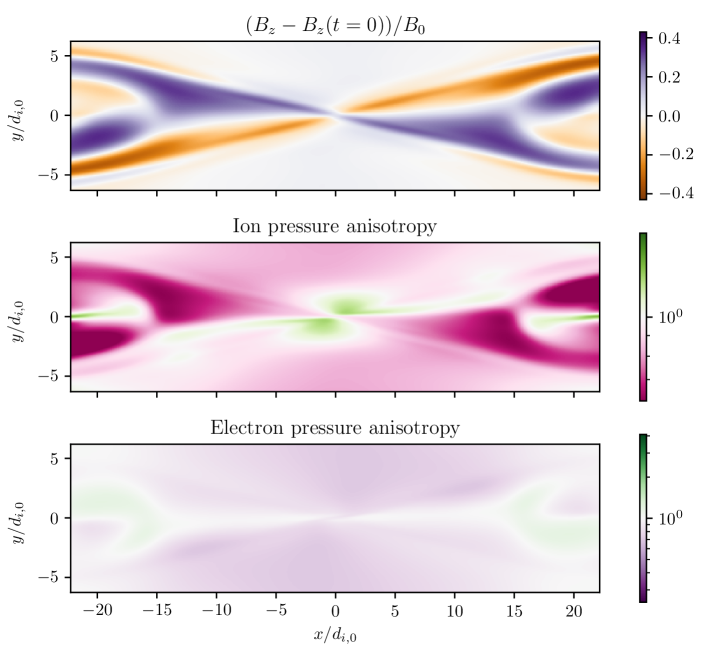
Figure 11: Hybrid 10-moment-Vlasov simulation of the reconnection setup from [53], state at $t=180\,\Omega_{i,0}^{-1}$. Shown are the deviation of the magnetic guide field from its initial value (top) and the species pressure anisotropies (middle, bottom).

Of course, the chosen mass ratio is not one where the hybrid model can exploit its full potential, and a far higher spatial resolution is possible as well. However, we want to use the same parameters as in [53] to make a direct comparison possible with the results therein and the respective models, which include a standard hybrid simulation (code HVM), the mentioned hybrid Landau fluid simulation (code HVLF, an extension of HVM) and a fully kinetic simulation using a semi-implicit PIC model (code iPIC3D). As opposed to these, the muphyII simulation that we present in this section has an exceptionally low computational cost, as we will point out. We want to elaborate on the physical differences between these models briefly. The HVM code uses the most common hybrid model with a quasi-neutral electron fluid, fully isotropic electron pressure, and a generalized Ohm’s law. The HVLF model also makes the quasi-neutral and generalized Ohm’s law approximations (including electron inertia) but evolves the gyrotropic pressure (i.e. the components parallel and perpendicular to the magnetic field) with a Landau fluid closure for the gyrotropic heat flux. In contrast, the muphyII hybrid model uses the ten-moment fluid equations for the electrons, which evolve the full pressure tensor with the temperature gradient heat flux closure to model Landau damping, and full Maxwell’s equations. Therefore, it self-consistently captures – alongside many other physical effects – electron inertia, charge separating plasma waves and light waves. The implemented heat flux closure is a general-purpose closure for collisionless wave damping, whereas the closure implemented in HVLF also considers the direction imposed by the magnetic field. Therefore, it is expected that the HVLF fluid closure is better suited for guide field reconnection (which is the setup in this section) but cannot be utilized for reconnection where the guide field is zero or close to zero (as in the previous sections). The iPIC3D code uses a fully kinetic model for both electrons and ions, as well as full Maxwell’s equations so that all physics can be represented and no approximation for heat flux is needed. At the given resolution, the implicitness of iPIC3D removes charge-separating waves and drives towards quasi-neutrality [53].

In Fig. 11 three quantities are shown that are relevant in estimating the model’s capabilities of capturing anisotropy: The magnetic field in guide field direction (difference from initial value) $\tilde{B_{z}}=B_{z}(t)-B_{z}(t=0)$, and the pressure anisotropies ${P_{\bot}}/{P_{\parallel}}$ for ions and electrons given by

$$\frac{P_{\perp}}{P_{\parallel}}=\frac{\sum_{i,j\in\{x,y,z\}}P_{ij}(\delta_{ij}-b_{i}b_{j})/2}{\sum_{i,j\in\{x,y,z\}}P_{ij}b_{i}b_{j}}\quad\text{where }b_{i}=B_{i}/|\mathbf{B}|,P_{ji}=P_{ij}$$

We compare the hybrid ten-moment electron, Vlasov ion results from muphyII with Figures 3 and 4 of [53], which represent the simulation data produced by the codes HVM, HVLF, and iPIC3D. The asymmetry in the spatial structure of $\tilde{B_{z}}=B_{z}(t)-B_{z}(t=0)$ shown in the top panel of Fig. 11 is caused to a large extent by the electron anisotropy and agrees very nicely with the fully kinetic results from iPIC3D, in particular around the Alfvénic front in the outflow region, where there are some differences between iPIC3D and the HVLF model. As expected, around the X-point this asymmetry is better represented in the HVLF simulation, which uses a heat flux closure that is well-suited for guide field reconnection. The HVM model, on the other hand, produces a nearly symmetrical result, which is in contrast with the kinetic findings.

The ion pressure anisotropy shows similarities between all models. Interestingly, both the hybrid ten-moment electron muphyII simulation (middle panel of Fig. 11) and the HVLF simulation have higher values of ion pressure anisotropy ${P_{\bot,i}}/{P_{\parallel,i}}$ in the Alfvénic outflow than the iPIC3D simulation. Whether this is caused by numerical differences between the Vlasov and the implicit PIC method, by different physics in the hybrid and the fully kinetic models, or simply by different states of the simulations cannot be settled here.

Last, we want to discuss the electron pressure anisotropy. The picture fits well with what already became clear from the analysis of the magnetic field in the guide field direction. The overall structure of electron pressure anisotropy in the hybrid ten-moment electron simulation (bottom panel of Fig. 11) differs from the iPIC3D result. The HVLF clearly performs better around the X-point, predicting lower values of ${P_{\bot,e}}/{P_{\parallel,e}}$, just as the fully kinetic model, and reproduces the elongation of the current sheet that is typically observed in guide field reconnection. This reverses around the Alfvénic front, where ${P_{\bot,e}}/{P_{\parallel,e}}>1$ in both the hybrid ten-moment electrons result from muphyII and the kinetic iPIC3D result, but not in HVLF. Both observations are to be expected, considering that the gyrotropic formulation of the HVLM electron closure excels in regions with a strong directional magnetic field, while the muphyII electron closure has been developed from the unmagnetized limit and has its strength in corresponding regions of low magnetization.

To summarize the results, it was shown that the hybrid ten-moment electron, Vlasov ion model performs to expectations in this guide field reconnection setup, although it was not tuned for the physical configuration in the slightest. More importantly, the muphyII hybrid simulation (which was run using only eight GPU cards) was computationally much cheaper than the simulations in [53]. The primary reason for this is that the matched-moments Vlasov solver can deal with the low velocity space resolution of $16^{3}$ cells. For comparison, the resolution used for the HVM and HVLF runs in [53] is $51^{3}$ cells for velocity space and would result in 32 times more degrees of freedom, and thus a 32 times higher computational effort for solving the Vlasov equation, though the actual runtime is not as easily comparable if the models’ numerical schemes and timestep requirements differ. Still, despite the considerably lower velocity resolution, there are no major qualitative differences in the ion results between the higher resolved HVM and HVLF runs and the lower resolved muphyII runs that cannot be attributed to the difference in electron models. That is no surprise either, as the higher resolution is primarily necessary for numerical reasons in classic Vlasov methods, and low velocity space resolutions have been used in PIC codes with much success since the beginning. Since the moment-matching approach is not dependent on numerical schemes of muphyII, and is transferable to other implementations like HVM and HVLF (with appropriate treatment of the second moment), we expect those models could benefit from its reduced computational footprint as well. A second performance aspect is that the heat flux closure in the HVLF model utilizes computations in Fourier space, which is much more expensive at large problem sizes than the local closure used by muphyII.

Through the use of electron and Maxwell subcycling and the moment-matched Vlasov solver, the novel hybrid model implemented in muphyII can represent detailed electron and electromagnetic physics in collisionless plasmas at very low computational cost.

6 Conclusions

In this paper, we have presented the multiphysics framework muphyII for simulations of collisionless plasmas in space and astrophysical environments. We interface-couple comparatively cheap fluid solvers with kinetic Vlasov solvers and employ the moment-matching approach, subcycling of Maxwell’s equations, and electron subcycling. As a result, the simulation of spatial regions that would not be treatable with Vlasov solvers alone is achieved. We have also shown that the moment-matching approach benefits the hybrid Vlasov-Fluid model in particular. In conclusion, this framework is an important step towards achieving the goal of global simulations from kinetic to magnetohydrodynamic (MHD) scales.

It can be even more rewarding to use the coupling of different plasma models in three-dimensional simulations. In 3D, depending on the physical problem, the portion of the spatial domain that can be covered by fluid models may be much larger than in 2D. muphyII has already been used for three-dimensional ten-moment fluid simulations [32], and the code fully supports coupled simulations in 3D, which we plan to utilize in the future. There, the matched-moments Vlasov solver will be of great value because it can reduce the large memory requirements that are inherent to the Vlasov method in three dimensions.

The future path to extending this framework is fairly obvious. To achieve true multiscale/multiphysics simulations, the coarsest model in our framework, the five-moment/Maxwell model, needs to be coupled with the MHD equations equipped with Ohm’s law and extended with adaptive mesh refinement (AMR). This is an ongoing work to combine the multiphysics framework muphyII and our multiscale framework racoon [36].

In addition, the framework muphyII allows but also needs further, more sophisticated implementations of refinement criteria. The design of these criteria, e.g. based on some form of suitably defined residuum, is a major mathematical challenge for this kind of simulations, not only in plasma physics.

Code Availability

The muphyII code is available on GitHub (https://github.com/muphy2-framework/muphy2) and Zenodo (https://zenodo.org/doi/10.5281/zenodo.8061586).

References

- [1] I. B. Peng, S. Markidis, A. Vaivads, J. Vencels, J. Amaya, A. Divin, E. Laure, G. Lapenta, The formation of a magnetosphere with implicit particle-in-cell simulations, Procedia Computer Science 51 (2015) 1178–1187, international Conference On Computational Science, ICCS 2015.
-
[2]
S. von Alfthan, D. Pokhotelov, Y. Kempf, S. Hoilijoki, I. Honkonen,
A. Sandroos, M. Palmroth,
Vlasiator:
First global hybrid-vlasov simulations of earth’s foreshock and
magnetosheath, Journal of Atmospheric and Solar-Terrestrial Physics 120
(2014) 24–35.
doi:https://doi.org/10.1016/j.jastp.2014.08.012.
URL https://www.sciencedirect.com/science/article/pii/S1364682614001916 - [3] P. Degond, F. Deluzet, D. Doyen, Asymptotic-preserving particle-in-cell methods for the Vlasov–Maxwell system in the quasi-neutral limit, Journal of Computational Physics 330 (2017) 467–492.
- [4] T. P. Schulze, P. Smereka, W. E, Coupling kinetic Monte-Carlo and continuum models with application to epitaxial growth, Journal of Computational Physics 189 (1) (2003) 197 – 211.
- [5] P. Le Tallec, F. Mallinger, Coupling Boltzmann and Navier-stokes equations by half fluxes, J. Comput. Phys. 136 (1997) 51–67.
- [6] S. Tiwari, A. Klar, An adaptive domain decomposition procedure for Boltzmann and Euler equations, J. Comput. Appl. Math. 90 (1998) 223–237.
- [7] A. Klar, H. Neunzert, J. Struckmeier, Transition from kinetic theory to macroscopic fluid equations: A problem for domain decomposition and a source for new algorithms, Transport Theor. Stat. 29 (2000) 93–106.
- [8] P. Degond, G. Dimarce, L. Mieussens, A multiscale kinetic-fluid solver with dynamic localization of kinetic effects, J. Comput. Phys. 229 (2010) 4907–4933.
- [9] S. Dellacherie, Kinetic-fluid coupling in the field of the atomic vapor isotopic separation: Numerical results in the case of a monospecies perfect gas, AIP Conf. Proc. 663 (2003) 947–956.
- [10] T. Goudon, S. Jin, J.-G. Liu, B. Yan, Asymptotic-preserving schemes for kinetic-fluid modeling of disperse two-phase flows, J. Comput. Phys. 246 (2013) 145–164.
- [11] S. Tiwari, A. Klar, S. Hardt, A. Donkov, Coupled solution of the Boltzmann and Navier-Stokes equations in gas-liquid two phase flow, Comput. Fluids 71 (2013) 283–296.
- [12] V. Kolobov, R. Arslanbekov, Towards adaptive kinetic-fluid simulations of weakly ionized plasmas, Journal of Computational Physics 231 (3) (2012) 839–869.
- [13] T. Sugiyama, K. Kusano, Multi-scale plasma simulation by the interlocking of magnetohydrodynamic model and particle-in-cell kinetic model, J. Comput. Phys. 227 (2) (2007) 1340–1352.
- [14] S. Markidis, P. Henri, G. Lapenta, K. Rönnmark, M. Hamrin, Z. Meliani, E. Laure, The fluid-kinetic particle-in-cell method for plasma simulations, Journal of Computational Physics.
- [15] L. K. S. Daldorff, G. Tóth, T. I. Gombosi, G. Lapenta, J. Amaya, S. Markidis, J. U. Brackbill, Two-way coupling of a global Hall magnetohydrodynamics model with a local implicit particle-in-cell model, J. Comput. Phys. 268 (2014) 236–254.
- [16] K. Makwana, R. Keppens, G. Lapenta, Two-way coupling of magnetohydrodynamic simulations with embedded particle-in-cell simulations, Computer Physics Communications 221 (2017) 81–94.
- [17] R. J. Walker, G. Lapenta, J. Berchem, M. El-Alaoui, D. Schriver, Embedding particle-in-cell simulations in global magnetohydrodynamic simulations of the magnetosphere, Journal of Plasma Physics 85 (2019) 905850109.
- [18] X. Wang, Y. Chen, G. Tóth, Global magnetohydrodynamic magnetosphere simulation with an adaptively embedded particle-in-cell model, Journal of Geophysical Research: Space Physics 127 (8) (2022) e2021JA030091. doi:https://doi.org/10.1029/2021JA030091.
- [19] X. Wang, Y. Chen, G. Tóth, Simulation of magnetospheric sawtooth oscillations: The role of kinetic reconnection in the magnetotail, Geophysical Research Letters 49 (15) (2022) e2022GL099638. doi:https://doi.org/10.1029/2022GL099638.
- [20] Y. Shou, V. Tenishev, Y. Chen, G. Toth, N. Ganushkina, Magnetohydrodynamic with adaptively embedded particle-in-cell model: Mhd-aepic, Journal of Computational Physics 446 (2021) 110656. doi:https://doi.org/10.1016/j.jcp.2021.110656.
- [21] S. Markidis, V. Olshevsky, G. Tóth, Y. Chen, I. B. Peng, G. Lapenta, T. Gombosi, Kinetic Modeling in the Magnetosphere, American Geophysical Union (AGU), 2021, Ch. 38, pp. 607–615.
- [22] M. Innocenti, G. Lapenta, S. Markidis, A. Beck, A. Vapirev, A multi level multi domain method for particle in cell plasma simulations, Journal of Computational Physics 238 (2013) 115–140.
- [23] A. Ho, I. A. M. Datta, U. Shumlak, Physics-based-adaptive plasma model for high-fidelity numerical simulations, Frontiers in Physics 6 (2018) 105.
- [24] K. Fujimoto, Multi-scale kinetic simulation of magnetic reconnection with dynamically adaptive meshes, Frontiers in Physics 6.
- [25] K. Papadakis, Y. Pfau-Kempf, U. Ganse, M. Battarbee, M. Alho, M. Grandin, M. Dubart, L. Turc, H. Zhou, K. Horaites, I. Zaitsev, G. Cozzani, M. Bussov, E. Gordeev, F. Tesema, H. George, J. Suni, V. Tarvus, M. Palmroth, Spatial filtering in a 6d hybrid-vlasov scheme to alleviate adaptive mesh refinement artifacts: a case study with vlasiator (versions 5.0, 5.1, and 5.2.1), Geoscientific Model Development 15 (20) (2022) 7903–7912.
- [26] H. Schmitz, R. Grauer, Kinetic Vlasov simulations of collisionless magnetic reconnection, Physics of Plasmas 13 (9) (2006) 092309. doi:10.1063/1.2347101.
- [27] H. Schmitz, R. Grauer, Comparison of time splitting and backsubstitution methods for integrating Vlasov’s equation with magnetic fields, Comp. Phys. Comm. 175 (2006) 86.
- [28] H. Schmitz, R. Grauer, Darwin-Vlasov simulations of magnetised plasmas, J. Comput. Phys. 214 (2006) 738–756.
- [29] M. Rieke, T. Trost, R. Grauer, Coupled Vlasov and two-fluid codes on GPUs, Journal of Computational Physics 283 (2015) 436 – 452. doi:10.1016/j.jcp.2014.12.016.
- [30] S. Lautenbach, R. Grauer, Multiphysics simulations of collisionless plasmas, Frontiers in Physics 6 (2018) 113. doi:10.3389/fphy.2018.00113.
- [31] Jülich Supercomputing Centre, JUWELS: Modular Tier-0/1 Supercomputer at the Jülich Supercomputing Centre, Journal of large-scale research facilities 5 (A135). doi:10.17815/jlsrf-5-171.
- [32] F. Allmann-Rahn, S. Lautenbach, R. Grauer, R. D. Sydora, Fluid simulations of three-dimensional reconnection that capture the lower-hybrid drift instability, Journal of Plasma Physics 87 (1) (2021) 905870115. doi:10.1017/S0022377820001683.
- [33] F. Allmann-Rahn, S. Lautenbach, R. Grauer, An energy conserving vlasov solver that tolerates coarse velocity space resolutions: Simulation of mms reconnection events, Journal of Geophysical Research: Space Physics 127 (2) (2022) e2021JA029976, e2021JA029976 2021JA029976. doi:https://doi.org/10.1029/2021JA029976.
- [34] F. Allmann-Rahn, R. Grauer, K. Kormann, A parallel low-rank solver for the six-dimensional vlasov-maxwell equations, arXiv e-prints (2022) arXiv:2201.03471.
- [35] F. Allmann-Rahn, T. Trost, R. Grauer, Temperature gradient driven heat flux closure in fluid simulations of collisionless reconnection, Journal of Plasma Physics 84 (3) (2018) 905840307. doi:10.1017/S002237781800048X.
- [36] J. Dreher, R. Grauer, Racoon: A parallel mesh-adaptive framework for hyperbolic conservation laws, Parallel Computing 31 (2005) 913.
-
[37]
D. Alvarez, JUWELS
cluster and booster: Exascale pathfinder with modular supercomputing
architecture at juelich supercomputing centre 7 A183–A183.
doi:10.17815/jlsrf-7-183.
URL https://jlsrf.org/index.php/lsf/article/view/183 - [38] D. Grošelj, S. S. Cerri, A. B. Navarro, C. Willmott, D. Told, N. F. Loureiro, F. Califano, F. Jenko, Fully kinetic versus reduced-kinetic modeling of collisionless plasma turbulence, The Astrophysical Journal 847 (1) (2017) 28. doi:10.3847/1538-4357/aa894d.
-
[39]
D. Grošelj, A. Mallet, N. F. Loureiro,
F. Jenko,
Fully kinetic
simulation of 3d kinetic alfvén turbulence, Phys. Rev. Lett. 120 (2018)
105101.
doi:10.1103/PhysRevLett.120.105101.
URL https://link.aps.org/doi/10.1103/PhysRevLett.120.105101 - [40] C. Cheng, G. Knorr, The integration of the Vlasov equation in configuration space, Journal of Computational Physics 22 (3) (1976) 330–351. doi:10.1016/0021-9991(76)90053-X.
- [41] F. Filbet, E. Sonnendrücker, P. Bertrand, Conservative numerical schemes for the Vlasov equation, Journal of Computational Physics 172 (1) (2001) 166 – 187. doi:10.1006/jcph.2001.6818.
- [42] A. Kurganov, D. Levy, A third-order semidiscrete central scheme for conservation laws and convection-diffusion equations, SIAM Journal on Scientific Computing 22 (4) (2000) 1461–1488. doi:10.1137/S1064827599360236.
- [43] C.-W. Shu, S. Osher, Efficient implementation of essentially non-oscillatory shock-capturing schemes, Journal of Computational Physics 77 (2) (1988) 439 – 471. doi:10.1016/0021-9991(88)90177-5.
- [44] J. Ng, A. Hakim, L. Wang, A. Bhattacharjee, An improved ten-moment closure for reconnection and instabilities, Physics of Plasmas 27 (8) (2020) 082106. doi:10.1063/5.0012067.
- [45] L. Wang, A. H. Hakim, A. Bhattacharjee, K. Germaschewski, Comparison of multi-fluid moment models with particle-in-cell simulations of collisionless magnetic reconnection, Physics of Plasmas 22 (1) (2015) 012108. doi:10.1063/1.4906063.
- [46] T. Trost, S. Lautenbach, R. Grauer, Enhanced conservation properties of Vlasov codes through coupling with conservative fluid models, arXiv e-prints (2017) arXiv:1702.00367.
-
[47]
F. Valentini, P. Trávníček, F. Califano, P. Hellinger, A. Mangeney,
A
hybrid-vlasov model based on the current advance method for the simulation of
collisionless magnetized plasma, Journal of Computational Physics 225 (1)
(2007) 753–770.
doi:https://doi.org/10.1016/j.jcp.2007.01.001.
URL https://www.sciencedirect.com/science/article/pii/S0021999107000022 -
[48]
F. Valentini, S. Servidio, D. Perrone, F. Califano, W. H. Matthaeus, P. Veltri,
Hybrid vlasov-maxwell simulations of
two-dimensional turbulence in plasmas, Physics of Plasmas 21 (8) (2014)
082307.
arXiv:https://doi.org/10.1063/1.4893301, doi:10.1063/1.4893301.
URL https://doi.org/10.1063/1.4893301 -
[49]
M. Palmroth, U. Ganse, Y. Pfau-Kempf, M. Battarbee, L. Turc, T. Brito,
M. Grandin, S. Hoilijoki, A. Sandroos, S. von Alfthan,
Vlasov methods in space
physics and astrophysics, Living Reviews in Computational Astrophysics 4 (1)
(2018) 1.
doi:10.1007/s41115-018-0003-2.
URL https://doi.org/10.1007/s41115-018-0003-2 -
[50]
H. Karimabadi, V. Roytershteyn, H. X. Vu, Y. A. Omelchenko, J. Scudder,
W. Daughton, A. Dimmock, K. Nykyri, M. Wan, D. Sibeck, M. Tatineni,
A. Majumdar, B. Loring, B. Geveci,
The link between shocks, turbulence,
and magnetic reconnection in collisionless plasmas, Physics of Plasmas
21 (6) (2014) 062308.
arXiv:https://doi.org/10.1063/1.4882875, doi:10.1063/1.4882875.
URL https://doi.org/10.1063/1.4882875 -
[51]
L. Franci, P. Hellinger, M. Guarrasi, C. H. K. Chen, E. Papini, A. Verdini,
L. Matteini, S. Landi,
Three-dimensional
simulations of solar wind turbulence with the hybrid code CAMELIA, Journal
of Physics: Conference Series 1031 (2018) 012002.
doi:10.1088/1742-6596/1031/1/012002.
URL https://doi.org/10.1088/1742-6596/1031/1/012002 - [52] A. Le, W. Daughton, H. Karimabadi, J. Egedal, Hybrid simulations of magnetic reconnection with kinetic ions and fluid electron pressure anisotropy, Physics of Plasmas 23 (3) (2016) 032114. doi:10.1063/1.4943893.
-
[53]
Finelli, F., Cerri, S. S., Califano, F., Pucci, F., Laveder, D.,
Lapenta, G., Passot, T.,
Bridging hybrid- and
full-kinetic models with landau-fluid electrons - i. 2d magnetic
reconnection, A&A 653 (2021) A156.
doi:10.1051/0004-6361/202140279.
URL https://doi.org/10.1051/0004-6361/202140279 -
[54]
A. Stanier, L. Chacón, A. Le,
A
cancellation problem in hybrid particle-in-cell schemes due to finite
particle size, Journal of Computational Physics 420 (2020) 109705.
doi:https://doi.org/10.1016/j.jcp.2020.109705.
URL https://www.sciencedirect.com/science/article/pii/S0021999120304794 - [55] R. B. Torbert, J. L. Burch, T. D. Phan, M. Hesse, M. R. Argall, J. Shuster, R. E. Ergun, L. Alm, R. Nakamura, K. J. Genestreti, D. J. Gershman, W. R. Paterson, D. L. Turner, I. Cohen, B. L. Giles, C. J. Pollock, S. Wang, L.-J. Chen, J. E. Stawarz, J. P. Eastwood, K. J. Hwang, C. Farrugia, I. Dors, H. Vaith, C. Mouikis, A. Ardakani, B. H. Mauk, S. A. Fuselier, C. T. Russell, R. J. Strangeway, T. E. Moore, J. F. Drake, M. A. Shay, Y. V. Khotyaintsev, P.-A. Lindqvist, W. Baumjohann, F. D. Wilder, N. Ahmadi, J. C. Dorelli, L. A. Avanov, M. Oka, D. N. Baker, J. F. Fennell, J. B. Blake, A. N. Jaynes, O. Le Contel, S. M. Petrinec, B. Lavraud, Y. Saito, Electron-scale dynamics of the diffusion region during symmetric magnetic reconnection in space, Science 362 (6421) (2018) 1391–1395. arXiv:https://science.sciencemag.org/content/362/6421/1391.full.pdf, doi:10.1126/science.aat2998.
- [56] T. K. M. Nakamura, K. J. Genestreti, Y.-H. Liu, R. Nakamura, W.-L. Teh, H. Hasegawa, W. Daughton, M. Hesse, R. B. Torbert, J. L. Burch, B. L. Giles, Measurement of the magnetic reconnection rate in the Earth’s magnetotail, Journal of Geophysical Research: Space Physics 123 (11) (2018) 9150–9168. doi:10.1029/2018JA025713.
- [57] K. J. Genestreti, T. K. M. Nakamura, R. Nakamura, R. E. Denton, R. B. Torbert, J. L. Burch, F. Plaschke, S. A. Fuselier, R. E. Ergun, B. L. Giles, C. T. Russell, How accurately can we measure the reconnection rate EM for the MMS diffusion region event of 11 July 2017?, Journal of Geophysical Research: Space Physics 123 (11) (2018) 9130–9149. arXiv:https://agupubs.onlinelibrary.wiley.com/doi/pdf/10.1029/2018JA025711, doi:10.1029/2018JA025711.
-
[58]
A. Le, J. Egedal, O. Ohia, W. Daughton, H. Karimabadi, V. S. Lukin,
Regimes of the
electron diffusion region in magnetic reconnection, Phys. Rev. Lett. 110
(2013) 135004.
doi:10.1103/PhysRevLett.110.135004.
URL https://link.aps.org/doi/10.1103/PhysRevLett.110.135004 - [59] P. A. Cassak, Y.-H. Liu, M. A. Shay, A review of the 0.1 reconnection rate problem, Journal of Plasma Physics 83 (5) (2017) 715830501. doi:10.1017/S0022377817000666.