MultiScale CUSUM Tests for Time-Dependent Spherical Random Fields

Abstract

This paper investigates the asymptotic behavior of structural break tests in the harmonic domain for time-dependent spherical random fields. In particular, we prove a Functional Central Limit Theorem result for the fluctuations over time of the sample spherical harmonic coefficients, under the null of isotropy and stationarity; furthermore, we prove consistency of the corresponding CUSUM test, under a broad range of alternatives. Our results are then applied to NCEP data on global temperature: our estimates suggest that Climate Change does not simply affect global average temperatures, but also the nature of spatial fluctuations at different scales.

AMS Classification: Primary: 62M40; Secondary: 62M30, 60G60
Keywords and Phrases: Time-Dependent Spherical Random Fields, Spherical Harmonics, Multiscale Cusum Test, Climate Change

1 Introduction

The analysis of time-dependent spherical random fields is the natural setting for a number of different areas of applications; some relevant examples include Cosmology, Geophysics and Atmospheric/Climate Sciences, among others, see for instance [7, 8, 10, 24, 25] and the references therein for a small sample of recent contributions (more generally, spherical data have been recently considered in different frameworks by [9, 11, 12, 15, 14], among others). In these areas, it is often a natural question to probe whether structural breaks have occurred over time; the most immediate example of such changes is obviously represented by shifts in the global mean, which would correspond to Global Warming when studying temperature data. Such shifts can be investigated by means of a number of traditional statistical tools, such as the celebrated CUSUM test for structural breaks.

Our purpose in this paper is to exploit harmonic/spectral methods to investigate MultiScale structural breaks, i.e., modifications of the statistical model which may go beyond a simple mean shift. A more rigorous and complete description of our environment will be given in the sections to follow; we believe, however, that it is useful to introduce from the start our motivations by means of a very preliminary analysis on a temperature data set.

In order to do so, let us first recall that a sphere-cross-time random field is simply a collection of random variables $\{T(x,t),\ (x,t)\in\mathbb{S}^{2}\times\mathbb{Z}\};$ under some regularity conditions (to be given below) the following Spectral Representation holds:

$$T(x,t)=\sum_{\ell=0}^{\infty}T_{\ell}(x,t)=\sum_{\ell=0}^{\infty}\sum_{m=-\ell}^{\ell}\beta_{\ell m}(t)Y_{\ell m}(x)\text{ ,}$$

where $\left\{Y_{\ell m},\ m=-\ell,\dots,\ell,\ \ell=0,1,2,\dots\right\}$ denotes the set of fully-normalized real spherical harmonics, an orthonormal basis for the space of square-integrable real-valued functions on the sphere, see [20]. Heuristically, each term $T_{\ell}(\cdot,t)$ can be viewed as the Fourier component of the spherical field at time $t$ when projected onto basis elements characterized by fluctuations of typical scale $\theta_{\ell}\simeq\pi/\ell$. In particular, the term corresponding to $\ell=0$ is simply the sample mean at time $t$ computed on the whole sphere; as such, it is for instance the typical statistic of interest when discussing global increments of the Earth Temperature. As already mentioned, our aim in this paper is to explore possible changes occurring at different scales; for instance, it could be the case that even when the global mean is unaltered, or in addition to changes in the latter, other modifications occur in the fluctuations of the variable of interest.

This point is illustrated by a simple, very preliminary data analysis that we report here just as a motivating example; much greater details will be given below in Section 4. More precisely, we consider global (land and ocean) surface temperature anomalies; the dataset is built starting from the NCEP/NCAR monthly averages of the surface air temperature (in degrees Celsius) from 1948 to 2020, over a global grid with $2.5^{\circ}$ spacing for latitude and longitude, see [19]. Following the World Meteorological Organization policy, temperature anomalies are obtained by subtracting the long-term monthly means relative to the 1981-2010 base period. They are then averaged over months to switch from a monthly scale to an annual scale (we refer also to the recent survey [26] for general discussion on the role of Statistics for Climate Data).

Figure 1 reports the temporal evolution of $\beta_{00}(t)$, which is nothing else than the sample average of Earth temperature at time $t$; unsurprisingly, this global mean grows steadily from 1949 to 2020.

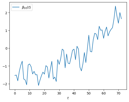
Figure 1: $\{\beta_{00}(t),\ t=1948,\dots,2020\}$.

Let us now consider a plot of the fluctuations of the temperature, with respect to its historical mean (given in Figure 2). A careful inspection of the colors suggests that not only some regions exhibit greater changes than others (i.e., the Poles), but also that a small periodic pattern seems to appear, with greater fluctuations that are at an approximated distance of 40-60 degrees across different latitudes.

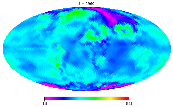
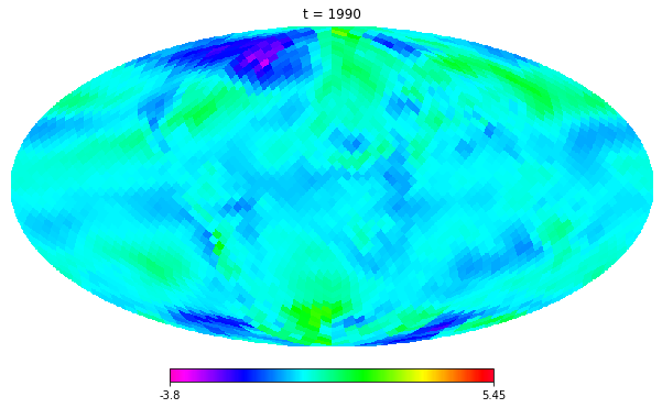
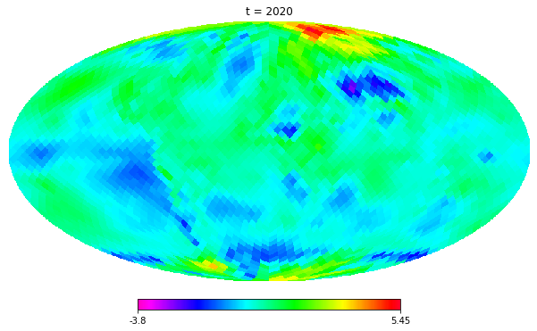
Figure 2: Global surface temperature anomalies at $t=1960,1990,2020$.

This point can be made clearer by introducing the spherical coordinates $\theta\in[0,\pi]$ (co-latitude) and $\phi\in[0,2\pi)$ (longitude); in this coordinates, the spectral representation becomes

$$T(\theta,\phi;t)=\sum_{\ell=0}^{\infty}T_{\ell}(\theta,\phi;t)=\sum_{\ell=0}^{\infty}\sum_{m=-\ell}^{\ell}\beta_{\ell m}(t)Y_{\ell m}(\theta,\phi)$$

with the analytic expressions

$$Y_{\ell m}(\theta,\phi) = \begin{dcases}\sqrt{\frac{2\ell+1}{2\pi}}\sqrt{\frac{(\ell-|m|)!}{(\ell+|m|)!}}P_{\ell|m|}(\cos\theta)\sin(|m|\phi)&\text{for }m<0\\ \sqrt{\frac{2\ell+1}{4\pi}}P_{\ell 0}(\cos\theta)&\text{for }m=0\\ \sqrt{\frac{2\ell+1}{2\pi}}\sqrt{\frac{(\ell-m)!}{(\ell+m)!}}P_{\ell m}(\cos\theta)\cos(m\phi)&\text{for }m\geq 0\end{dcases},$$

$$P_{\ell m}(u) = \frac{1}{2^{\ell}\ell!}(1-u^{2})^{m/2}\frac{d^{\ell+m}}{dt^{\ell+m}}(u^{2}-1)^{\ell},u\in[-1,1].$$

The $P_{\ell m}$’s are the well-known associated Legendre functions, whereas the $\beta_{\ell m}(t)$’s can be obtained by means of the Fourier transform

$$\int_{-\pi}^{\pi}\int_{0}^{\pi}T_{\ell}(\theta,\phi;t)Y_{\ell m}(\theta,\phi)\sin\theta d\theta d\phi.$$ (1.1)

Note also that, for every $\ell=0,1,2,\dots,$ we have that

$$\int_{-\pi}^{\pi}T_{\ell}(\theta,\phi;t)d\phi = \sqrt{2\ell+1}\sqrt{\pi}\beta_{\ell 0}(t)P_{\ell 0}(\cos\theta)\text{ .}$$

In other words, up to a deterministic function, each random process $\left\{\beta_{\ell 0}(t),\ t\in\mathbb{Z}\right\}$ captures the temporal evolution of the sample spatial mean for the spectral component corresponding to the multipole $\ell$, computed at any given latitude. To explore their behavior, we plot in Figure 3 the observed evolution of $\beta_{\ell 0}(t)$ over the time span 1948-2020, for $\ell=2,4,6,8,$. It is remarkable that these coefficients appear indeed to grow over time, suggesting that further changes in the Earth temperature pattern may have occurred, in addition to the growth of the global average.

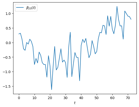
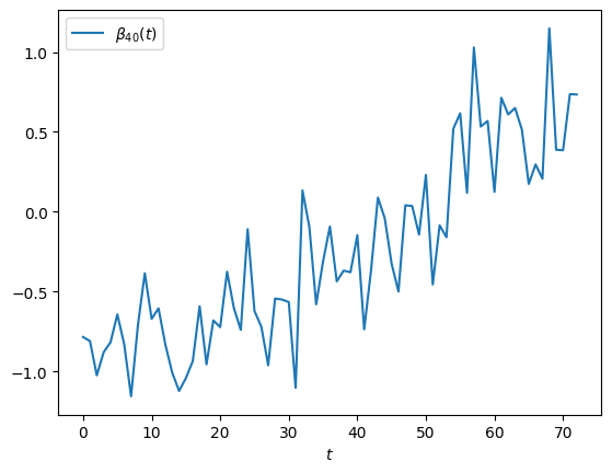
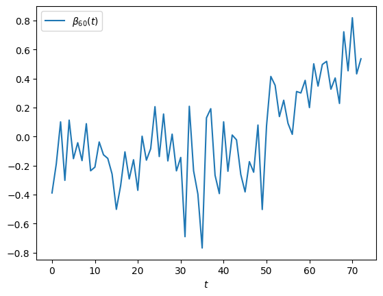
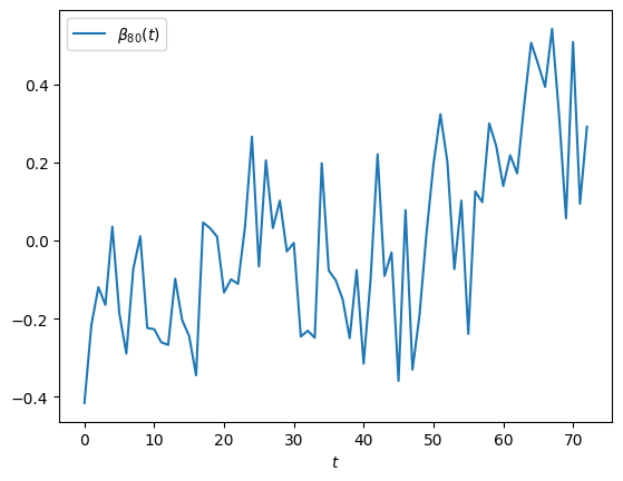
Figure 3: $\{\beta_{\ell 0}(t),\ t=1948,\dots,2020\},$ for $\ell=2,4,6,8$.

This preliminary data exploration suggests that even if we were to subtract the global temperature mean from each time observation, in order to make it constantly equal to zero, the effects of Climate Change would still be visible in the form of structural changes on different scales. Our purpose in this paper is to devise a class of tests in order to investigate these phenomena more rigorously, which is what we start to do from the next section.

2 Model

In this section, we introduce our model of interest. In short, under the null we assume to be dealing with a collection of Gaussian time-dependent spherical random fields with a stationary (in time) but anisotropic (in space) mean function; we are going to probe alternatives that replace the stationary mean by introducing time-varying factors which may vary across the different multipole components.

Let $\{Z(x,t),\ (x,t)\in\mathbb{S}^{2}\times\mathbb{Z}\}$ denote a centered Gaussian isotropic and stationary sphere-cross-time random field, that is, a collection of jointly Gaussian random variables with finite variance and such that

$$\mathbb{E}[Z(x,t)] = 0,$$

$$\mathbb{E}[Z(x_{1},t_{1})Z(x_{2},t_{2})] =: \Gamma(\langle x_{1},x_{2}\rangle,t_{2}-t_{1}),$$

with $\langle\cdot,\cdot\rangle$ being the standard inner product in $\mathbb{R}^{3}$. As anticipated above, it is well-known (see, e.g., [20]) that the space of square-integrable functions on the sphere admits as an orthonormal basis the fully-normalized spherical harmonics $\left\{Y_{\ell m},\ m=-\ell,\dots,\ell,\ \ell=0,1,2,\dots\right\}$, which are eigenfunctions of the spherical Laplacian and hence they satisfy the Helmholtz equation

$$\Delta_{\mathbb{S}^{2}}Y_{\ell m}=-\lambda_{\ell}Y_{\ell m}\text{ , }\qquad\lambda_{\ell}=\ell(\ell+1)\text{ , }\qquad\ell=1,2,\dots,$$

$$\Delta_{\mathbb{S}^{2}}=\frac{1}{\sin\theta}\frac{\partial}{\partial\theta}\left(\sin\theta\frac{\partial}{\partial\theta}\right)+\frac{1}{\sin^{2}\theta}\frac{\partial^{2}}{\partial\phi^{2}}\text{ .}$$

The Spectral Representation Theorem for isotropic random fields ensures that, in $L^{2}(\Omega\times\mathbb{S}^{2})$

$$Z(\theta,\phi;t)=\sum_{\ell=0}^{\infty}\sum_{m=-\ell}^{\ell}a_{\ell m}(t)Y_{\ell m}(\theta,\phi).$$

The idea is now to consider a process $\{T(x,t),\ (x,t)\in\mathbb{S}^{2}\times\mathbb{Z}\}$ that satisfies

$$T(x,t)-\mu(x)=Z(x,t),$$ (2.1)

for some deterministic $\mu(\cdot)\in L^{2}(\mathbb{S}^{2})$. The anisotropic (but stationary) mean function then has the $L^{2}$-expansion

$$\mu(\theta,\phi) = \sum_{\ell=0}^{\infty}\sum_{m=-\ell}^{\ell}\mu_{\ell m}Y_{\ell m}(\theta,\phi)\text{ ,}$$

$$\mu_{\ell m} = \int_{-\pi}^{\pi}\int_{0}^{\pi}\mu(\theta,\phi)Y_{\ell m}(\theta,\phi)\sin\theta d\theta d\phi\text{ .}$$

Hence, we can introduce our model under the null hypothesis in the next Assumption.

Assumption 2.1.

Under the null $H_{0}$, the field satisfies the equation in (2.1), and hence it is Gaussian with stationary mean function $\mathbb{E}[T(x,t)]=\mu(x)$, and has spectral representation

$$T(x,t)=\sum_{\ell=0}^{\infty}\sum_{m=-\ell}^{\ell}a_{\ell m}(t)Y_{\ell m}(x)+\sum_{\ell=0}^{\infty}\sum_{m=-\ell}^{\ell}\mu_{\ell m}Y_{\ell m}(x)\text{ .}$$

Under the assumptions on $\{Z(x,t),\ (x,t)\in\mathbb{S}^{2}\times\mathbb{Z}\}$ we also have that the array of spherical harmonic coefficients $\{a_{\ell m}(t),\ m=-\ell,\dots,\ell,\ \ell=0,1,2,\dots,\ t\in\mathbb{Z}\}$ is formed by zero-mean Gaussian independent (over $\ell$ and $m$) and stationary (over $t$) processes, with covariances and spectral density functions given by

$$C_{\ell}(\tau) :=\mathbb{E}[a_{\ell m}(t+\tau)a_{\ell m}(t)]\text{ ,}\qquad t,\tau\in\mathbb{Z},$$

$$f_{\ell}(\lambda) :=\frac{1}{2\pi}\sum_{\tau\in\mathbb{Z}}C_{\ell}(\tau)e^{-i\lambda\tau}\text{ , }\qquad\lambda\in[-\pi,\pi]\text{ .}$$

Note that $\{C_{\ell}(0),\ \ell=0,1,2,\dots\}$ corresponds to the angular power spectrum of the spherical field at a given time point, for which we will simply write $\{C_{\ell},\ \ell=0,1,2,\dots\}$ . We also impose the following regularity conditions on the behavior of these spectral densities.

Assumption 2.2.

The sequence of spectral densities $f_{\ell}(\cdot)$ is such that

$$0<c\leq\liminf_{\ell=1,2,\dots}\min_{\lambda\in[-\pi,\pi]}\frac{f_{\ell}(\lambda)}{C_{\ell}}\leq\limsup_{\ell=1,2,\dots}\max_{\lambda\in[-\pi,\pi]}\frac{f_{\ell}(\lambda)}{C_{\ell}}\leq c^{\prime}<\infty\text{ .}$$ (2.2)

In words, we need to require that the spectral densities, once normalized to integrate to one, are uniformly bounded above and below (away from zero). This is a mild non-degeneracy condition on the temporal dependence of the spherical harmonic coefficients; it would fail, for instance, if for some $\ell$ the process $\{a_{\ell 0}(t),\ t\in\mathbb{Z}\}$ would exhibit long memory behavior or follow a non-invertible stationary process, such as an over-differenced $MA(q)$.

We shall here introduce our model under the alternative; in this case, we allow the deterministic mean function to vary over time, and hence we consider a process $\{T(x,t),\ (x,t)\in\mathbb{S}^{2}\times\mathbb{Z}\}$ that satisfies

$$T(x,t)-\mu(x,t)=Z(x,t),$$ (2.3)

for some $\mu(\cdot,t)\in L^{2}(\mathbb{S}^{2})$, $t\in\mathbb{Z}$.

Assumption 2.3.

Under the alternative $H_{1}$, the field satisfies the equation in (2.3), so that

$$T(x,t)=\sum_{\ell=0}^{\infty}\sum_{m=-\ell}^{\ell}a_{\ell m}(t)Y_{\ell m}(x)+\sum_{\ell=0}^{\infty}\sum_{m=-\ell}^{\ell}\mu_{\ell m}(t)Y_{\ell m}(x)\text{ .}$$

Moreover, there exist a sequence of non-negative real numbers $\{\alpha_{\ell},\ \ell=0,1,2,\dots\}$ and $\overline{\alpha}:=\max_{\ell=0,1,\dots}\alpha_{\ell}>0$ such that the following expansion holds

$$\mu_{\ell m}(t)=\mu_{\ell m;0}+\mu_{\ell m;1}\times t^{\alpha_{\ell}}+\mu_{\ell m;2}(t)\text{ , }$$

where $\sum_{\ell,m}\mu_{\ell m;i}^{2}<\infty$, for $i=0,1,2$,

$$\sum_{m=-\ell}^{\ell}\mu_{\ell m;1}\neq 0\text{ , for }\ell\in\mathcal{I}\text{ ,}\qquad\lim_{t\rightarrow\infty}\frac{\mu_{\ell m;2}(t)}{t^{\alpha_{\ell}-\epsilon}}=0\text{ , for some }\epsilon>0,$$

and $\mathcal{I}$ is the set of indexes $\{\ell:\alpha_{\ell}=\overline{\alpha}\}$.

Remark 2.4.

This condition is satisfied for instance when $\mu_{\ell m;2}(t)=t^{\alpha_{\ell}-\epsilon^{*}}\log t^{k}$, for some $\epsilon^{*}>0$ and some $k\in\mathbb{R}$.

The alternative we are considering introduces a growing algebraic trend (to the leading order) which can be different from multipole to multipole and can be assumed arbitrarily small. This model seems very general and able to capture a number of nonparametric alternatives; of course, further power terms or oscillating components are allowed in the remainder term. We are back to the model under the null either by taking $\mu_{\ell m;i}\equiv 0$, $i=1,2$, or by taking $\overline{\alpha}=0$ and $\mu_{\ell m}\equiv\mu_{\ell m;0}+\mu_{\ell m;1}$, for all values of $\ell$ and $m$. The set $\mathcal{I}$ can be viewed as the collection of multipoles which exhibit the strongest non-linear trend; we are imposing that these multipoles have coefficients which do not sum to zero, otherwise the condition is clearly meaningless.

2.1 The Test Statistic

We are now ready to introduce our proposed statistics; it can also be viewed as a form of Fourier domain testing for stationarity for functional valued time series, see [2, 17].

In this paper, we adopt the simplifying assumption that the field is fully observed on a grid of values that corresponds to a suitable pixelization on the sphere, such as the one implemented by the HEALPix scheme (see [16]). Under this assumption, it is possible to compute the Fourier coefficients and evaluate the following test statistic.

Definition 2.5.

(Sample Harmonic Coefficients) For $t=1,2,\dots,N$, the sample spherical harmonic coefficients are defined by

$$\beta_{\ell m}(t):=\int_{S^{2}}T(x,t)Y_{\ell m}(x)dx\text{ ;}$$

Definition 2.6.

(Sample Harmonic Averages) The harmonic averages are defined as

$$\widehat{\mu}_{\ell m}:=\frac{1}{N}\sum_{t=1}^{N}\beta_{\ell m}(t)\text{ .}$$

Definition 2.7.

(Sample Power Spectrum) The sample power spectrum is defined as

$$\overline{C}_{\ell}:=\frac{1}{N(2\ell+1)}\sum_{t=1}^{N}\sum_{m=-\ell}^{\ell}(\beta_{\ell m}(t)-\widehat{\mu}_{\ell m})^{2}\text{ .}$$

Remark 2.8.

We are here implicitly assuming that the $\beta_{\ell m}(t)$’s can be estimated exactly from the observations, i.e., that the integrals defined in (1.1) can be computed without approximations. We will discuss the role of these approximations below in Subsection 2.2.

Definition 2.9.

The Test Statistic Let $L=L(N)$ be a growing sequence of natural numbers, whose exact expression will be discussed below; let also $0\leq\underline{L}$ be a fixed integer value. The test statistic on which we shall focus is

$$A_{L,N}(r,s):=\frac{1}{\sqrt{N}}\frac{1}{\sqrt{L}}\sum_{t=1}^{[Ns]}\sum_{\ell=\underline{L}}^{[Lr]}\frac{1}{\sqrt{2\ell+1}}\sum_{m=-\ell}^{\ell}\frac{\beta_{\ell m}(t)-\widehat{\mu}_{\ell m}}{\sqrt{\overline{C}_{\ell}}},\qquad r,s\in[0,1]\text{ .}$$

The asymptotic behavior of the test statistic under the Null and Alternative Hypothesis will be discussed in the following section. The next subsection is instead devoted to a brief technical discussion on the issue of pixelization. It should be noted that the statistic $A_{L,N}(\cdot,\cdot)$ depends on the choice of $\underline{L}$; however the limiting behavior is independent from the choice of any (fixed) $\underline{L}$, and hence this parameter does not appear in $A_{L,N}(\cdot,\cdot)$ to make the notation lighter.

2.2 The Role of Pixelization

Throughout this paper, we assume that the spherical harmonic coefficients can be computed by means of exact integrals. As mentioned earlier, in practice this is not going to be feasible in general: in practice, it is likely that only a finite number of observations will be sampled on $\mathbb{S}^{2}$ and integrals will be approximated by Riemann sums on the sphere. We shall show below that for random fields with a regular angular power spectrum (to be defined below) and a careful approach to asymptotics, replacing integrals over the sphere with sums over a finite regular grid does not affect limiting distributions.

Definition 2.10.

We say that the set of points $\{\xi_{L^{*},k},\ k=1,\dots,n_{L^{*}}\}$ and weights $\{\lambda_{L^{*},k},\ k=1,\dots,n_{L^{*}}\}$ are cubature points and cubature weights (respectively) of order $L^{*}$ if we have, for all $\ell\leq L^{*}$,

$$\sum_{k=1}^{n_{L^{*}}}Y_{\ell m}(\xi_{L^{*}k})Y_{\ell^{\prime}m^{\prime}}(\xi_{L^{*}k})\lambda_{L^{*},k}=\int_{\mathbb{S}^{2}}Y_{\ell m}(x)Y_{\ell^{\prime}m^{\prime}}(x)dx=\delta_{\ell}^{\ell^{\prime}}\delta_{m}^{m^{\prime}}.$$

In words, cubature points and weights of order $L^{*}$. provide a finite grid on which integrals of spherical harmonics can be computed exactly as a finite sum with suitable weights, up to the order $\ell<L^{*}$. The possibility to construct cubature points and weights on the sphere $\mathbb{S}^{2}$ is a classical result in approximation theory and harmonic analysis, see for instance [22] for a proof and [3, 21, 23, 27] for further discussions; it is also known that these points can be shown to be nearly equi-spaced with cardinality of order $(L^{*})^{2}$ and weights of nearly constant magnitude (over $k$), i.e., $c_{1}/(L^{*})^{2}<\lambda_{L^{*},k}<c_{2}/(L^{*})^{2}$, for some $c_{1},c_{2}>0$. In practice, the cubature points correspond to the centers of standard pixelizations on the sphere, such as those provided by the very popular package HEALPix ([16]); hereafter we shall hence assume that our data are exactly located on those points, that is, we assume to observe $\{T(\xi_{L^{*}k},t)$,  $k=1,2,\dots,n_{L^{*}}$, $t=1,\dots,N$} (in this Subsection, we take for simplicity the mean term $\mu$ to be identically equal to zero). The spherical harmonic coefficients can be then estimated up to some multipole $L\leq L^{*}$ by

$$\beta^{*}_{\ell m}(t):=\sum_{k=1}^{n_{L^{*}}}T(\xi_{L^{*}k},t)Y_{\ell m}(\xi_{L^{*}k})\lambda_{L^{*},k}.$$

The crucial idea is that the exact spherical harmonic transforms can be replaced by their discretized version provided the maximum order of $\ell$ does not grow too quickly with respect to what the order of pixelization allows to do. This idea is made rigorous in the following Assumption.

Definition 2.11.

For a given angular power spectrum $\{C_{\ell},\text{ }\ell=1,2,\dots\}$, we say that the growing sequences $L=L(N)<L^{*}=L^{*}(N)$ are jointly regular (with respect to $\{C_{\ell},\text{ }\ell=1,2,\dots\})$ if as $N\rightarrow\infty,$ we have that

$$\frac{1}{C_{L(N)}}\sum_{\ell=L^{*}(N)+1}^{\infty}(2\ell+1)C_{\ell}=O(L^{-\delta}(N))\text{ , some $\delta>0.$}$$

We say also that the sequences $L=L(N)<L^{*}=L^{*}(N)$ are strongly jointly regular (with respect to $\{C_{\ell},\text{ }\ell=1,2,\dots\})$ if as $N\rightarrow\infty,$ we have that

$$\frac{L^{2}(N)}{C_{L(N)}}\sum_{\ell=L^{*}(N)+1}^{\infty}(2\ell+1)C_{\ell}=O(L^{-\delta}(N))\text{ , some $\delta>0.$}$$

Remark 2.12.

Let us assume (as usual) that the angular power spectrum satisfies a regularity condition

$$\lim_{\ell\rightarrow\infty}\frac{C_{\ell}}{\ell^{-\eta}}=const>0\text{ ,}\quad\text{for some }\eta>2\text{ .}$$

It is then easy to show that a jointly regular pair is obtained by taking $L,L^{*}$ such that $L^{\zeta}=O(L^{*})$, for $\zeta=\frac{\eta}{\eta-2}+\delta$, any $\delta>0$. Indeed, in this case one obtains

$$L^{\eta}\sum_{\ell=L^{*}+1}^{\infty}\ell^{-\eta+1}=O(L^{\eta}(L^{*})^{-\eta+2})=O(L^{\eta}L^{(-\eta+2)\zeta})=o(1)\text{ , }\text{as }N\rightarrow\infty\text{ .}$$

By the same argument it is immediately seen that strong joint regularity holds for $\zeta=\frac{\eta+2}{\eta-2}+\delta$.

These conditions show that for rapidly decreasing power spectra ($\eta>>0$) the parameter $\zeta$ can be taken arbitrarily close to 1 and still obtain jointly regular sequences. As we shall show below, this entails that a (relatively) large proportion of multipoles $\ell$ can be used for statistical data analysis without substantial effects due to the pixelization scheme. On the contrary, for $\eta$ closer to 2 only a small fraction of the computable multipoles should be used for statistical analysis if we want to make sure that pixelization effects are negligible. For cosmological experiments (e.g., CMB data, [13]) the decay of the power spectrum is known to be nearly exponential (due to the so-called Silk damping effect) for values of the multipoles in the order of $\ell\sim 10^{4}$, so that pixelizations effects are likely to be negligible in that domain.

Now, consider the following decomposition (for $\ell\leq L<L^{*}$)

$$\beta^{*}_{\ell m}(t)=\sum_{k=1}^{n_{L^{*}}}\left\{T_{L^{*}}(\xi_{L^{*}k},t)+R_{L^{*}}(\xi_{L^{*}k},t)\right\}Y_{\ell m}(\xi_{L^{*}k})\lambda_{L^{*}k}=\beta_{\ell m}(t)+r^{*}_{\ell m}(t)\text{ ,}$$

where

$$T_{L^{*}}(\xi_{L^{*}k},t) = \sum_{\ell=0}^{L^{*}}\sum_{m=-\ell}^{\ell}\beta_{\ell m}(t)Y_{\ell m}(\xi_{L^{*}k})\text{ ,}$$

$$R_{L^{*}}(\xi_{L^{*}k},t) = \sum_{\ell=L^{*}+1}^{\infty}\sum_{m=-\ell}^{\ell}\beta_{\ell m}(t)Y_{\ell m}(\xi_{L^{*}k})\text{ ,}$$

$$r^{*}_{\ell m}(t) = \sum_{k=1}^{n_{L^{*}}}R_{L^{*}}(\xi_{L^{*}k},t)Y_{\ell m}(\xi_{L^{*}k})\lambda_{L^{*}k}\text{ .}$$

Intuitively, we have split the field into two components; on the first the spherical harmonic transform can be computed exactly, for the second we shall show that it is uniformly and almost surely negligible in the asymptotic limit. The variance of the reminder term $r^{*}_{\ell m}(t)$ is easily seen to be

$$\operatorname{Var}\left[r^{*}_{\ell m}(t)\right]\leq\sum_{k=1}^{n_{L^{*}}}\operatorname{Var}[R_{L^{*}}(\xi_{L^{*}k},t)]\lambda_{L^{*}k}=\sum_{\ell=L^{*}+1}^{\infty}\frac{2\ell+1}{4\pi}C_{\ell}\text{ .}$$

Then, we have the following.

Lemma 2.13.

For jointly regular sequences $L(N),L^{*}(N)$ and $N=O(L^{\gamma})$, any $\gamma>0$, we have that

$$\limsup_{L(N)\rightarrow\infty}\sup_{t=1,\dots,N}\sup_{\ell=1,\dots,L(N)}\sup_{m=-\ell,\dots,\ell}\frac{\beta^{*}_{\ell m}(t)-\beta_{\ell m}(t)}{\sqrt{C_{\ell}}}=0\text{ with probability 1 .}$$

Proof.

By Mill’s inequality we have that

$$\mathbb{P}\left(\frac{\beta^{*}_{\ell m}(t)-\beta_{\ell m}(t)}{\sqrt{C_{\ell}}}>\epsilon\right)=\mathbb{P}\left(z^{*}_{\ell m}(t)>\epsilon\right)\leq\frac{\sigma_{z_{\ell m}}}{\epsilon}\exp\left\{-\epsilon^{2}/2\sigma^{2}_{z_{\ell m}}\right\}\text{ , }$$

where $z^{*}_{\ell m}(t):=\frac{\beta^{*}_{\ell m}(t)-\beta_{\ell m}(t)}{\sqrt{C_{\ell}}}$, and $\sigma^{2}_{z_{\ell m}}:=\operatorname{Var}\left[z^{*}_{\ell m}(t)\right]$. For jointly regular sequences, one has immediately that

$$\sup_{\ell=1,\dots,L(N)}\sup_{m=-\ell,\dots,\ell}\sigma^{2}_{z_{\ell m}}=O(L^{-\delta}(N)),\text{ some }\delta>0\text{ , }$$

whence for any $\epsilon>0$

$$\mathbb{P}\left(\bigcup_{t=1,\dots,N}\bigcup_{\ell=1,\dots,L(N)}\bigcup_{m=-\ell,\dots,\ell}\{\omega:z_{\ell m}(\omega)>\epsilon\}\right)$$

$$\leq\sum_{t=1,\dots,N}\sum_{\ell=1,\dots,L(N)}\sum_{m=-\ell,\dots,\ell}\mathbb{P}\left(\{\omega:z_{\ell m}(\omega)>\epsilon\}\right)$$

$$\leq L^{\gamma}\times L(2L+1)\sup_{t=1,\dots,N}\sup_{\ell=1,\dots,L(N)}\sup_{m=-\ell,\dots,\ell}\mathbb{P}\left(\{\omega:z_{\ell m}(\omega)>\epsilon\}\right)$$

$$\leq L^{\gamma}\times L(2L+1)\frac{1}{L^{-\delta/2}\epsilon}\exp\left\{-\frac{1}{2}\epsilon^{2}L^{\delta}\right\}=O\left(L^{\gamma+2-\delta/2}\exp\left\{-\frac{1}{2}\epsilon^{2}L^{\delta}\right\}\right)\text{ , }$$

and thus the proof is completed by a standard Borel-Cantelli argument. ∎

In words, the Lemma is stating that approximating the spherical harmonic coefficients by means of their approximations with a finite sum rather than an integral has a negligible effect asymptotically, provided the angular power spectrum is smooth enough and a slowly growing sequence of multipoles is considered.

We shall now give a stronger, functional version of the approximation result; here for simplicity we shall assume that the angular power spectrum of the field is known, so that we can replace the estimate ${\overline{C}_{\ell}}$ with the theoretical values $C_{\ell}$ in the test statistic $A_{L,N}(\cdot,\cdot)$.

Let us define

$$A_{L,N;L^{*}}(r,s)=\frac{1}{\sqrt{N}}\frac{1}{\sqrt{L}}\sum_{t=1}^{[Ns]}\sum_{\ell=1}^{[Lr]}\frac{1}{\sqrt{2\ell+1}\sqrt{C}_{\ell}}\sum_{m=-\ell}^{\ell}r^{*}_{\ell m}(t)\text{ .}$$

Clearly this process represents the component of our test statistic which is due to the approximation error induced by the pixelization; it would be identically equal to zero if we had access to the exact values $\{\beta_{\ell m}(t),\ m=-\ell,\dots,\ell,\ \ell=1,2,\dots,L,\ t=1,\dots,N\}$.

Lemma 2.14.

As $N\rightarrow\infty$, we have that, for $L,L^{*}$ strongly joint regular

$$\sup_{r,s\in[0,1]}|A_{L,N;L^{*}}(r,s)|\rightarrow 0\text{ , almost surely .}$$

Proof.

It is immediate that $A_{L,N;L^{*}}(r,s)$ is Gaussian with expected value zero and variance bounded by

$$\mathbb{E}\left[A_{L,N;L^{*}}^{2}(r,s)\right]$$

$$=\frac{1}{NL}\sum_{t_{1},t_{2}=1}^{[Ns]}\sum_{\ell_{1},\ell_{2}=1}^{[Lr]}\frac{1}{\sqrt{2\ell_{1}+1}\sqrt{C_{\ell_{1}}}}\frac{1}{\sqrt{2\ell_{2}+1}\sqrt{C_{\ell_{2}}}}\sum_{m_{1}=-\ell_{1}}^{\ell_{1}}\sum_{m_{2}=-\ell_{2}}^{\ell_{2}}\mathbb{E}\left[r_{\ell_{1}m_{1}}(t_{1})r_{\ell_{2}m_{2}}(t_{2})\right]$$

$$\leq Const\times\frac{1}{L}\sum_{\ell_{1},\ell_{2}=1}^{[Lr]}\frac{(2\ell_{1}+1)}{\sqrt{2\ell_{1}+1}\sqrt{C_{\ell_{1}}}}\frac{(2\ell_{2}+1)}{\sqrt{2\ell_{2}+1}\sqrt{C_{\ell_{2}}}}\frac{1}{N}\sum_{t_{1},t_{2}=1}^{[Ns]}\sum_{\ell=L^{*}+1}^{\infty}(2\ell+1)C_{\ell}(t_{2}-t_{1})$$

$$\leq Const\times\frac{1}{L}\sum_{\ell_{1},\ell_{2}=1}^{[Lr]}\frac{(2\ell_{1}+1)}{\sqrt{2\ell_{1}+1}\sqrt{C_{\ell_{1}}}}\frac{(2\ell_{2}+1)}{\sqrt{2\ell_{2}+1}\sqrt{C_{\ell_{2}}}}\sum_{\ell=L^{*}+1}^{\infty}(2\ell+1)C_{\ell}$$

$$\leq Const\times L^{2}\frac{1}{C_{L}}\sum_{\ell=L^{*}+1}^{\infty}(2\ell+1)C_{\ell}=:\sigma_{r,L,L^{*}}^{2}$$

Now we can use either the Borell-TIS inequality, or the Landau-Shepp inequality (which is less efficient but simpler) – see, e.g., [1]. By this we can show that

$$\mathbb{P}\left(\sup_{r,s\in[0,1]}|A_{L,N;2}(r,s)|>\varepsilon\right)\leq\exp\left\{\left(\delta-\frac{1}{\sigma_{r,L,L^{*}}^{2}}\right)\varepsilon^{2}\right\}\text{ , for all }\delta>0\text{ .}$$

The proof is once again completed by a Borel-Cantelli argument, provided that we show that the tail variance $\sigma_{r,L,L^{*}}^{2}=O(L^{-\delta})$, some $\delta>0$; this is an immediate consequence of the strong regularity condition on $L,L^{*}$. ∎

3 Main Results

To characterize the limiting distribution of our statistic of interest under the null, we introduce one more definition.

Definition 3.1.

A Brownian pillowcase is a zero-mean Gaussian process $W:[0,1]^{2}\rightarrow\mathbb{R}$ with covariance function

$$\mathbb{E}[W(r,s)W(r^{\prime},s^{\prime})]=(r\wedge r^{\prime})((s\wedge s^{\prime})-ss^{\prime}).$$

It is immediate to see that for $r=1$ or $s=1$ the Brownian pillowcase coincides with the standard Brownian bridge and Brownian motion, respectively. We are now in the position to state our two main results, which establish the behavior of our test statistic under the null and the alternative assumptions, respectively.

Theorem 3.2.

Under Assumption 2.1 and 2.2, as $N\rightarrow\infty$ and $L=L(N)\rightarrow\infty,$

$$A_{L,N}(r,s)\Longrightarrow W(r,s)\text{ ,}$$

where $\Longrightarrow$ denotes as usual weak convergence in the Skorohod space $D[0,1]^{2}$.

The previous result ensures the weak convergence under the null of our test statistic; threshold values for the excursion of Kolmogorov-Smirnov or Cramér-Von Mises statistics can hence be derived by analytic computations or simulations. Our next result ensures that the corresponding test are asymptotically consistent, meaning that the probability of Type II errors converges to zero as the number of observations grow.

Theorem 3.3.

Under Assumption 2.3, as $N\rightarrow\infty$ ($L=L(N)),$ for all $M>0$,

$$\mathbb{P}\left(\sup_{r,s\in[0,1]}\left|A_{L,N}(r,s)\right|>M\right)\rightarrow 1\,.$$

The proofs of these two Theorems are given in Appendix A and B, respectively. Let us discuss shortly the role of the Assumptions that we introduced:

a) the assumption of Gaussianity allows some convenient simplifications when computing higher-order moments, which are needed in particular when we establish tightness conditions (in particular, we exploit the power of Wick’s diagram formula ([1])). In principle, this assumption can be relaxed and replaced by conditions on the fourth-order cumulant spectra of the random spherical harmonic coefficients: the computations are likely however to become considerably heavier, because under non-Gaussianity it is no longer the case that the spherical harmonic sequences are independent across different multipoles $\ell,\ell^{\prime}$; hence the terms to consider in the higher order moments would grow very significantly.

b) it is possible to consider alternative forms of non-stationarity under the alternative assumption. However it is not clear that this would indeed represent a substantial generalization, as the power model we are considering can be viewed as a Taylor approximation of a much wider class of functions.

c) it is important that we allow for different values of $\underline{L}$, as this gives the opportunity to neglect the effect of any fixed number of low order multipoles. More explicitly, this allows to probe the presence of non-stationarity behavior neglecting the effect of global changes in the mean or changes at the larger scales. This possibility is exploited in our data analysis below, where we drop sequentially the first multipoles and show that, even neglecting changes in the global mean, climate changes are still strongly supported by the observed data. Indeed, there is evidence for modifications in the behavior for temperature data at least for the first 10 multipoles $\ell$, that is, down to scales in the order of 20 degrees or smaller.

In the sections to follow, we illustrate the validity of these results by means of an extensive Monte Carlo study and an application to the NCEP Temperature Data.

4 Numerical Results and Applications to NCEP Data

4.1 Approximating the Rejection Threshold

Since the quantiles of $\sup_{r,s\in[0,1]}|W(r,s)|$ are not explicitly available, we approximate the rejection threshold by a small Monte Carlo experiment. We base the approximation on a well-known asymptotic result, see for instance [18]. Indeed we simulate independently a Brownian motion and a Brownian bridge both on a grid of $300$ equally-spaced points on the unit interval and we take their outer product. This returns a matrix of $300\times 300$ products. We replicate these steps $n=10000$ times and then we average all the obtained matrices. In the end, we compute the absolute value of all the elements in the averaged matrix and we take the maximum among them. The whole procedure is repeated to obtain a sample of size $B=2000$ and from this the Monte Carlo approximation of the distribution (see Figure 4) and the selected quantiles, which are

• $q_{0.90}=1.2911$ at level $0.90$;

• $q_{0.95}=1.4142$ at level $0.95$;

• $q_{0.99}=1.7104$ at level $0.99$.

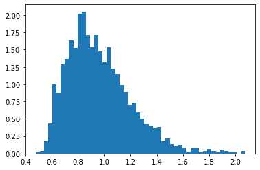
Figure 4: Histogram of the limiting Brownian pillowcase.

4.2 Simulations Under $H_{0}$

Here we exploit HEALPix [16] to generate $N$ independent and identically distributed Gaussian isotropic random fields on the sphere, through the simulations of their first $L$ harmonic coefficients

$$\{a_{\ell m}(t),\ m=-\ell,\dots,\ell,\ \ell=0,\dots,L,\ t=1,\dots,N\}.$$

Each simulated coefficient is then the realization of

$$a_{\ell m}(t)\sim\mathcal{N}(0,C_{\ell}(0)),\quad\text{where }C_{\ell}(0)=\frac{2}{\ell(\ell+1)}.$$

We restrict our attention here to the independent case, but actually one can also consider some form of stationarity among the coefficients that satisfies our assumptions, see for instance [6, 8].

Recall that under $H_{0}$,

$$\beta_{\ell m}(t)=a_{\ell m}(t)+\mu_{\ell m}.$$

We then consider three different scenarios

1. the global mean $\mu(\cdot)$ is constant and equal to 5;

2. $\mu_{00}=5$, $\mu_{\ell 0}=-\frac{2}{\ell(\ell+1)}$ for $\ell$ even, zero the rest of the coefficients;

3. $\mu_{00}=5$, $\mu_{\ell 0}=-\frac{2}{\ell(\ell+1)}$ for all $\ell=1,\dots,L$, zero the rest of the coefficients.

We first fix $N=100,\ L=30$, and we compute the test statistic under Models 1,2,3 on a grid of $300\times 300$ equally-spaced points on the unit square, for $B=2000$ replications. Figures 5 and 6 show respectively one realization of $A_{L,N}(\cdot,\cdot)$ and the approximate distribution of the sup test statistic, while Table 1 reports the approximate Type one error probability associated with the selected quantiles.

We then repeat the experiment ($B=1000$) choosing higher $N$ and $L=100$. Comparing now Table 2 with Table 1, we can observe that the Type one error probability is closer to the target values, as expected.

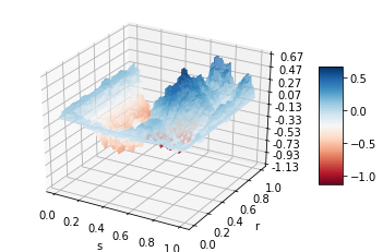
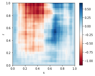
Figure 5: Realization of $A_{L,N}$ under Model 2 at $N=100$ ($L=30$).

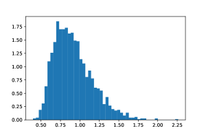
Figure 6: Histogram of the sup test statistic under Model 2 at $N=100$ $(L=30)$ based on $B=2000$ replicates.

Model	$q_{0.90}$	$q_{0.95}$	$q_{0.99}$
1	0.064	0.033	0.0055
2	0.081	0.0415	0.0055
3	0.084	0.0455	0.006

Table 1: Type I error probability ($N=100,\ L=30$) based on $B=2000$ replicates.

Model	$N$	$q_{0.90}$	$q_{0.95}$	$q_{0.99}$
1	700	0.093	0.054	0.007
2	500	0.091	0.043	0.008
3	300	0.106	0.056	0.009

Table 2: Type I error probability ($L=100$) based on $B=1000$ replicates.

4.3 Simulations Under $H_{1}$

Let us now focus on the alternative hypothesis; under $H_{1}$, the global mean depends on time, i.e.,

$$\beta_{\ell m}(t)=a_{\ell m}(t)+\mu_{\ell m}(t).$$

For the residuals we consider the same Gaussian model used under $H_{0}$, while for the mean we can consider a temporal modification of scenarios 1-2-3 in Section 4.2:

1. $\mu_{00}(t)=5\cdot t^{\alpha}$, while the remaining coefficients are set to zero;

2. $\mu_{00}=5\cdot t^{\alpha}$, $\mu_{\ell 0}=-\frac{2}{\ell(\ell+1)}\cdot t^{\alpha}$ for $\ell$ even, while the remaining coefficients are set to zero;

3. $\mu_{00}=5\cdot t^{\alpha}$, $\mu_{\ell 0}=-\frac{2}{\ell(\ell+1)}\cdot t^{\alpha}$ for all $\ell=1,\dots,L$, while the remaining coefficients are set to zero.

In particular we focus on the second model with $\alpha=0.5$. Results are obtained by fixing $N=100,300,500,$ $L=30$, and computing the test statistic on a grid of $300\times 300$ equally-spaced points on the unit square, for $B=2000$ replications. Figure 7 shows three realizations of $A_{L,N}(\cdot,\cdot)$ under Model 2 with $\alpha=0.5$ when $N=100,300,500$ respectively.

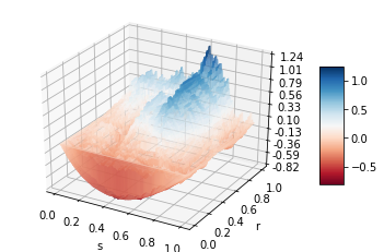
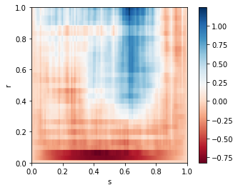
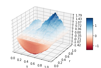
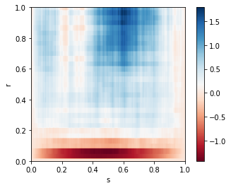
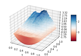
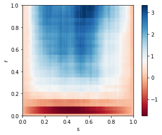
Figure 7: Realizations of $A_{L,N}$ under Model 2 ($\alpha=0.5$) at $N=100,300,500$ – from top to bottom.

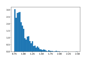
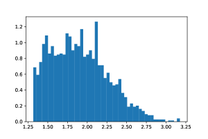
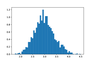
Figure 8: Histograms of the sup test statistic under Model 2 ($\alpha=0.5$) at $N=100,300,500$ – from top to bottom.

The approximate test’s power is reported in Table 3. As expected, for higher values of $\alpha$, the probability of rejection under $H_{1}$ approaches one at smaller sample sizes. Figure 8 illustrates in particular how the distribution of the sup test statistic under $H_{1}$ changes when increasing the number of time-observations $N$.

$\alpha$	$N$	$q_{0.90}$	$q_{0.95}$	$q_{0.99}$
	100	0.0975	0.055	0.0145
0.5	300	1.0	0.934	0.670
	500	1.0	1.0	1.0
1	100	1.0	1.0	1.0

Table 3: Test’s power under Model 2.

4.4 Application to NCEP Data

As mentioned in the Introduction, the above methodology was applied to global (land and ocean) surface temperature anomalies. More in detail, the dataset is built starting from the NCEP/NCAR monthly averages of the surface air temperature (in degrees Celsius) from 1948 to 2020, over a global grid with $2.5^{\circ}$ spacing for latitude and longitude, see [19]. We recall again that, following the World Meteorological Organization policy, temperature anomalies are obtained by subtracting the long-term monthly means relative to the 1981-2010 base period; they are then averaged over months to switch from a monthly scale to an annual scale.

By means of the HEALPix package (see [16] and the official HEALPix website), we converted the gridded data into spherical maps with a resolution of $12\cdot\operatorname{NSIDE}^{2}$ pixels (NSIDE = 16) and then we computed the Fourier coefficients up to $L=2\cdot\operatorname{NSIDE}$.

The observed value of the sup test statistic is about 5.1 (see also Figure 9), which strongly suggests to reject the null hypothesis of a stationary (in time) mean function.

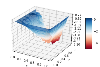
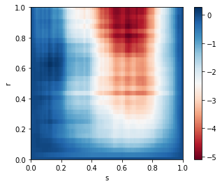
Figure 9: Observed test statistic.

We now run the same test, neglecting the multipole $\ell=0$, that is, subtracting at each time $t$ the global sample average of the temperature, which is then made constant over time. We repeat then the same approach, by dropping in turn the first L-1 multipoles, for L=2,4,6,8: this way we explore the existence of non-stationarity features that do not involve the mean or the following lowest multipoles. Our test statistic is still significant (see Table 4) in each of these cases, suggesting that climate changes occurs not only in the mean temperature at a global level, but also in the nature of fluctuations on a number of different scales corresponding to a few dozen degrees. The meaning and consequences of these preliminary findings on the nature of non-stationarity for climate data are left for future investigations.

L	0	1	2	4	6	8
sup	5.1	4.5	4.08	3.38	3.0	2.67

Table 4: Empirical results on NCEP data

5 Appendix A: Proof of Theorem 3.2

The main idea in the proof is to split our test statistic into two different parts; in the first, the normalization is implemented by means of the (unknown) theoretical power spectrum, whereas in the second we collect a remainder term that compares the statistic under the theoretical normalization with the "studentized" version, where the normalization is implemented by means of the sample variance of the estimated spherical coefficients. More precisely, we have the following identity:

$$A_{L,N}(r,s)=A_{1;L,N}(r,s)+A_{2;L,N}(r,s)\,,$$

where

$$A_{1;L,N}(r,s)=\frac{1}{\sqrt{N}}\frac{1}{\sqrt{L}}\sum_{t=1}^{[Ns]}\sum_{\ell=1}^{[Lr]}\frac{1}{\sqrt{2\ell+1}}\sum_{m=-\ell}^{\ell}\frac{\beta_{\ell m}(t)-\widehat{\mu}_{\ell m}}{\sqrt{C_{\ell}}}$$

and

$$A_{2;L,N}(r,s)=\frac{1}{\sqrt{N}}\frac{1}{\sqrt{L}}\sum_{t=1}^{[Ns]}\sum_{\ell=1}^{[Lr]}\frac{1}{\sqrt{2\ell+1}}\sum_{m=-\ell}^{\ell}\left(\frac{\beta_{\ell m}(t)-\widehat{\mu}_{\ell m}}{\sqrt{\overline{C}_{\ell}}}-\frac{\beta_{\ell m}(t)-\widehat{\mu}_{\ell m}}{\sqrt{C_{\ell}}}\right)\,.$$

A first difficulty to deal with is the fact that a random quantity appears at the denominator, and hence we need precise lower bounds in order to ensure that the corresponding moments do not diverge. These lower bounds are discussed in the next subsection.

5.1 On the Distribution of $\overline{C}_{\ell}$

Let $\mathbf{X}=\left(X_{1},\dots,X_{N}\right)^{\prime}$ be a vector of $N$ observations collected at times $1,\dots,N$ of a second-order stationary process with expected value $\mu$; then each $X_{t}$ can be expressed as follows

$$X_{t}=\frac{1}{\sqrt{N}}\sum_{j=0}^{N-1}\alpha_{j}e^{it\omega_{j}},\qquad\omega_{j}=\frac{2\pi j}{N},\quad\omega_{j}\in[0,2\pi),$$

where

$$\alpha_{j}=\alpha(\omega_{j})=\frac{1}{\sqrt{N}}\sum_{t=1}^{N}X_{t}e^{-i\omega_{j}t}\,;$$

note that $\mathbb{E}\left[X_{t}\right]=\mu$, $\mathbb{E}\left[\alpha_{0}\right]=\sqrt{N}\mu$ and $\mathbb{E}\left[\alpha_{j}\right]=0$, for each $j=1,\dots,N$; the $\alpha_{j}$ are the well-known Discrete Fourier Transforms of our observations – see, e.g., [5]. As a consequence,

$$\sum_{t=1}^{N}X_{t}^{2}=\sum_{j=0}^{N-1}\left\lvert\alpha_{j}\right\rvert^{2}=\sum_{j=0}^{N-1}2\pi I(\omega_{j}),\qquad\text{as }\quad 2\pi I(\omega_{j}):=\left\lvert\alpha_{j}\right\rvert^{2}\,,$$

where we have written as usual $I(\omega_{j})$ for the periodogram of $X_{t}$ evaluated on the Fourier frequencies $\omega_{j}$, $j=1,\dots,N$. Moreover, it is well-known (see [5]) and easy to check that

$$\alpha_{0}=\frac{1}{\sqrt{N}}\sum_{t=1}^{N}X_{t}=\sqrt{N}\,\widebar{X}_{N}\implies\left\lvert\alpha_{0}\right\rvert^{2}=N\,\widebar{X}_{N}^{2}\,,$$

so that

$$\sum_{t=1}^{N}\left(X_{t}-\widebar{X}_{N}\right)^{2}=\sum_{t=1}^{N}X_{t}^{2}-N\,\widebar{X}_{N}^{2}=\sum_{j=1}^{N-1}I(\omega_{j}),$$

and hence

$$\frac{1}{N}\sum_{t=1}^{N}\left(X_{t}-\widebar{X}_{N}\right)^{2}=\frac{1}{N}\sum_{j=1}^{N-1}I(\omega_{j})=\frac{1}{N}\sum_{j=1}^{N-1}\left\lvert\alpha_{j}\right\rvert^{2}\,.$$

It is now convenient to introduce a vector/matrix notation and define

$$\mathbf{v}_{j}=\frac{1}{\sqrt{N}}\left(e^{-i\omega_{j}\cdot 1},\dots,e^{-i\omega_{j}\cdot N}\right),$$

so that

$$\alpha_{j}=\frac{1}{\sqrt{N}}\sum_{t=1}^{N}X_{t}e^{-i\omega_{j}t}=\mathbf{v}_{j}\mathbf{X},$$

and

$$\mathbf{A}=\left(\begin{array}[]{c}\alpha_{1}\\ \vdots\\ \alpha_{N-1}\end{array}\right)=\left(\begin{array}[]{c}\mathbf{v}_{1}\\ \vdots\\ \mathbf{v}_{N-1}\end{array}\right)\mathbf{X}=\mathbf{V\,X}\,.$$

We can then consider the covariance matrix

$$\Sigma=\mathbb{E}\left[\mathbf{A}\mathbf{A}^{\ast}\right]=\mathbb{E}\left[\mathbf{V}\mathbf{XX}^{\prime}\mathbf{V}^{\ast}\right]=\mathbf{V}\mathbb{E}\left[\mathbf{XX}^{\prime}\right]\mathbf{V}^{\ast}=\mathbf{V}\Gamma\mathbf{V}^{\ast}\,.$$

Therefore, for the sample variance of $\mathbf{X}$ we have

$$S =\frac{1}{N}\sum_{t=1}^{N}\left(X_{t}-\widebar{X}_{N}\right)^{2}=\frac{1}{N}\mathbf{A}^{\ast}\mathbf{A}=\frac{1}{N}\mathbf{Z}^{\ast}\Sigma\mathbf{Z}$$

$$=\frac{1}{N}\mathbf{Z}^{\ast}\mathbf{V}\Gamma\mathbf{V}^{\ast}\mathbf{Z}\geq\frac{1}{N}\lambda_{\min}\left(\Gamma\right)\mathbf{Z}^{\ast}\mathbf{Z}$$

$$=\frac{1}{N}\lambda_{\min}\left(\widetilde{\Gamma}+\mu^{2}\mathbf{1}_{N\times N}\right)\mathbf{Z}^{\ast}\mathbf{Z}\geq\frac{1}{N}\lambda_{\min}\left(\widetilde{\Gamma}\right)\mathbf{Z}^{\ast}\mathbf{Z}\,,$$

where $\mathbf{Z}$ is a $(N-1)$-dimensional complex standard Gaussian random vector and $\widetilde{\Gamma}=\mathbb{E}\left[\mathbf{(X-\mu)(X-\mu)}^{\prime}\right]$.

Let us set

$$X_{t}=X_{t}^{\ell m}=\beta_{\ell m}(t),\quad\mu=\mu_{\ell m},\quad\widebar{X}_{N}=\widehat{\mu}_{\ell m},$$

$$S=S_{\ell m}=\frac{1}{N}\sum_{t=1}^{N}(\beta_{\ell m}(t)-\widehat{\mu}_{\ell m})^{2},$$

we are interested in computing $\mathbb{E}\left[\left(C_{\ell}/\overline{C}_{\ell}\right)^{4}\right]$, where

$$\frac{\overline{C}_{\ell}}{C_{\ell}}=\frac{1}{(2\ell+1)C_{\ell}}\sum_{m=-\ell}^{\ell}\frac{1}{N}\sum_{t=1}^{N}(\beta_{\ell m}(t)-\widehat{\mu}_{\ell m})^{2}=\frac{1}{(2\ell+1)C_{\ell}}\sum_{m=-\ell}^{\ell}S_{\ell m}\,.$$

From the computation above, we have that

$$\frac{\overline{C}_{\ell}}{C_{\ell}} =\frac{1}{(2\ell+1)C_{\ell}}\sum_{m=-\ell}^{\ell}S_{\ell m}\geq\frac{1}{2\ell+1}\sum_{m=-\ell}^{\ell}\frac{1}{T}\frac{\lambda_{\min}(\widetilde{\Gamma}_{\ell})}{C_{\ell}}\mathbf{Z}_{\ell m}^{\ast}\mathbf{Z}_{\ell m}$$

$$\geq c\frac{1}{2\ell+1}\frac{1}{T}\underbrace{\sum_{m=-\ell}^{\ell}\sum_{t=1}^{N}\left\lvert Z_{\ell m}(t)\right\rvert^{2}}_{\chi^{2}_{(N-1)(2\ell+1)}}\,,$$

provided that

$$\frac{\lambda_{\min}(\widetilde{\Gamma}_{\ell})}{C_{\ell}}\geq c.$$

The last inequality follows from Assumption 2.2; it is indeed well-known that the eigenvalues of the covariance matrix of a stationary process are bounded below from the minimum of their spectral densities, which in turn we assumed to be uniformly bounded from below after normalizing the variances of the spherical harmonic coefficients to unity. As a consequence

$$\mathbb{E}\left[\left(\frac{C_{\ell}}{\overline{C}_{\ell}}\right)^{4}\right]\leq c^{4}(2\ell+1)^{4}N^{4}\mathbb{E}\left[\left(\chi^{-2}_{(N-1)(2\ell+1)}\right)^{4}\right]=\frac{c^{4}(2\ell+1)^{4}N^{4}}{\prod_{k=1}^{4}\left((N-1)(2\ell+1)-2k\right)}\leq c^{\prime}\,,$$

where the bound is uniform in $\ell$.

5.2 On the Mean-Square Convergence of $\overline{C}_{\ell}/C_{\ell}$ to 1

Now consider

$$\left(\frac{\overline{C}_{\ell}}{C_{\ell}}-1\right)$$

$$=\frac{1}{N(2\ell+1)}\sum_{t=1}^{N}\sum_{m=-\ell}^{\ell}\frac{a^{2}_{\ell m}(t)+2(\mu_{\ell m}-\widehat{\mu}_{\ell m})a_{\ell m}(t)+(\mu_{\ell m}-\widehat{\mu}_{\ell m})^{2}}{C_{\ell}}-1$$

$$= \frac{1}{N(2\ell+1)}\sum_{t=1}^{N}\sum_{m=-\ell}^{\ell}\left(\frac{a^{2}_{\ell m}(t)}{C_{\ell}}-1\right)$$

$$+\frac{1}{N(2\ell+1)}\sum_{t=1}^{N}\sum_{m=-\ell}^{\ell}\frac{2(\mu_{\ell m}-\widehat{\mu}_{\ell m})a_{\ell m}(t)}{C_{\ell}}$$

$$+\frac{1}{2\ell+1}\sum_{m=-\ell}^{\ell}\frac{(\mu_{\ell m}-\widehat{\mu}_{\ell m})^{2}}{C_{\ell}}$$

$$=: V_{1;\ell,N}+V_{2;\ell,N}+V_{3;\ell,N}\text{ .}$$

Note that

$$\mathbb{E}[V_{1;\ell,N}] = 0\text{ ,}$$

$$\mathbb{E}[V_{2;\ell,N}] = \frac{1}{N(2\ell+1)}\sum_{t=1}^{N}\sum_{m=-\ell}^{\ell}\frac{2\mathbb{E}[\mu_{\ell m}-\widehat{\mu}_{\ell m}]a_{\ell m}(t)}{C_{\ell}}$$

$$= \frac{2}{N^{2}}\sum_{t=1}^{N}\sum_{s=1}^{N}\frac{C_{\ell}(t-s)}{C_{\ell}}$$

$$= \frac{2}{N}\sum_{\tau=-N+1}^{N-1}\left(1-\frac{|\tau|}{N}\right)\frac{C_{\ell}(\tau)}{C_{\ell}}\simeq\frac{4\pi}{N}\frac{f_{\ell}(0)}{C_{\ell}}\text{ ,}$$

where by $\simeq$ we mean that the ratio between the left- and right-hand sides tends to one as $N\rightarrow\infty$. Likewise

$$\mathbb{E}[V_{3;\ell,N}]=\frac{1}{2\ell+1}\sum_{m=-\ell}^{\ell}\frac{\mathbb{E}\left[(\mu_{\ell m}-\widehat{\mu}_{\ell m})^{2}\right]}{C_{\ell}}\simeq\frac{2\pi}{N}\frac{f_{\ell}(0)}{C_{\ell}}\text{ .}$$

Moreover, by triangle inequality it is immediate to see that

$$\mathbb{E}\left[\left(\frac{\overline{C}_{\ell}}{C_{\ell}}-1\right)^{2}\right]=\left\|\frac{\overline{C}_{\ell}}{C_{\ell}}-1\right\|_{L^{2}(\Omega)}^{2}$$

$$\leq\left(\left\|V_{1;\ell,N}\right\|_{L^{2}(\Omega)}+\left\|V_{2;\ell,N}\right\|_{L^{2}(\Omega)}+\left\|V_{3;\ell,N}\right\|_{L^{2}(\Omega)}\right)^{2}\text{ .}$$

We also have that

$$\left\|V_{1;\ell,N}\right\|_{L^{2}(\Omega)}^{2} = \left\|\frac{1}{N(2\ell+1)}\sum_{t=1}^{N}\sum_{m=-\ell}^{\ell}\left(\frac{a^{2}_{\ell m}(t)}{C_{\ell}}-1\right)\right\|_{L^{2}(\Omega)}^{2}$$

$$= \frac{2}{N}\sum_{\tau=-N+1}^{N-1}\left(1-\frac{|\tau|}{N}\right)\frac{C_{\ell}^{2}(\tau)}{C_{\ell}^{2}}\simeq\frac{2}{N}\int_{-\pi}^{\pi}\frac{f^{2}_{\ell}(\lambda)}{C^{2}_{\ell}}d\lambda.$$

Likewise

$$\left\|V_{2;\ell,N}\right\|_{L^{2}(\Omega)}^{2} = \left\|\frac{1}{N(2\ell+1)}\sum_{t=1}^{N}\sum_{m=-\ell}^{\ell}\frac{2(\mu_{\ell m}-\widehat{\mu}_{\ell m})a_{\ell m}(t)}{C_{\ell}}\right\|_{L^{2}(\Omega)}^{2}$$

$$= \frac{4}{N^{2}(2\ell+1)^{2}}\sum_{t_{1},t_{2}=1}^{N}\sum_{m_{1},m_{2}=-\ell}^{\ell}\frac{\mathbb{E}\left[(\mu_{\ell m_{1}}-\widehat{\mu}_{\ell m_{1}})a_{\ell m_{1}}(t_{1})(\mu_{\ell m_{2}}-\widehat{\mu}_{\ell m_{2}})a_{\ell m_{2}}(t_{2})\right]}{C_{\ell}^{2}}$$

$$= \frac{4}{N^{4}(2\ell+1)^{2}}\sum_{t_{1},t_{2}=1}^{N}\sum_{m_{1},m_{2}=-\ell}^{\ell}\frac{\mathbb{E}\left[\sum_{s_{1}=1}^{N}a_{\ell m_{1}}(s_{1})a_{\ell m_{1}}(t_{1})\sum_{s_{2}=1}^{N}a_{\ell m_{2}}(s_{2})a_{\ell m_{2}}(t_{2})\right]}{C_{\ell}^{2}}$$

$$= \frac{4}{N^{4}(2\ell+1)^{2}}\sum_{t_{1},t_{2}=1}^{N}\sum_{m_{1}\neq m_{2}}\sum_{s_{1}=1}^{N}\sum_{s_{2}=1}^{N}\frac{\mathbb{E}\left[a_{\ell m_{1}}(s_{1})a_{\ell m_{1}}(t_{1})a_{\ell m_{2}}(s_{2})a_{\ell m_{2}}(t_{2})\right]}{C_{\ell}^{2}}$$

$$+\frac{4}{N^{4}(2\ell+1)^{2}}\sum_{t_{1},t_{2}=1}^{N}\sum_{m=-\ell}^{\ell}\sum_{s_{1}=1}^{N}\sum_{s_{2}=1}^{N}\frac{\mathbb{E}\left[a_{\ell m}(s_{1})a_{\ell m}(t_{1})a_{\ell m}(s_{2})a_{\ell m}(t_{2})\right]}{C_{\ell}^{2}}$$

$$= \frac{4}{N^{4}}\frac{2\ell}{2\ell+1}\sum_{t_{1},t_{2}=1}^{N}\sum_{s_{1}=1}^{N}\sum_{s_{2}=1}^{N}\frac{C_{\ell}(t_{1}-s_{1})C_{\ell}(t_{2}-s_{2})}{C_{\ell}^{2}}$$

$$+\frac{4}{N^{4}}\frac{1}{2\ell+1}\sum_{t_{1},t_{2}=1}^{N}\sum_{s_{1}=1}^{N}\sum_{s_{2}=1}^{N}\frac{3C_{\ell}(t_{1}-s_{1})C_{\ell}(t_{2}-s_{2})}{C_{\ell}^{2}}$$

$$= \frac{4}{N^{4}}\frac{2\ell+3}{2\ell+1}\sum_{t_{1},t_{2}=1}^{N}\sum_{s_{1}=1}^{N}\sum_{s_{2}=1}^{N}\frac{C_{\ell}(t_{1}-s_{1})C_{\ell}(t_{2}-s_{2})}{C_{\ell}^{2}}\simeq\frac{4}{N^{2}}\frac{2\ell+3}{2\ell+1}\frac{f^{2}_{\ell}(0)}{C^{2}_{\ell}}\,.$$

Finally for the last term we obtain

$$\left\|V_{3;\ell,N}\right\|_{L^{2}(\Omega)}^{2} = \left\|\frac{1}{2\ell+1}\sum_{m=-\ell}^{\ell}\frac{(\mu_{\ell m}-\widehat{\mu}_{\ell m})^{2}}{C_{\ell}}\right\|_{L^{2}(\Omega)}^{2}$$

$$= \frac{1}{(2\ell+1)^{2}}\sum_{m_{1},m_{2}=-\ell}^{\ell}\frac{\mathbb{E}\left[\left(\frac{1}{N}\sum_{t_{1}=1}^{N}a_{\ell m_{1}}(t_{1})\right)^{2}\left(\frac{1}{N}\sum_{t_{2}=1}^{N}a_{\ell m_{2}}(t_{2})\right)^{2}\right]}{C_{\ell}^{2}}$$

$$= \frac{1}{N^{4}(2\ell+1)^{2}}\sum_{m_{1},m_{2}=-\ell}^{\ell}\sum_{t_{1},s_{1}=1}^{N}\sum_{t_{2},s_{2}=1}^{N}\frac{\mathbb{E}\left[a_{\ell m_{1}}(t_{1})a_{\ell m_{1}}(s_{1})a_{\ell m_{2}}(t_{2})a_{\ell m_{2}}(s_{2})\right]}{C_{\ell}^{2}}$$

$$\simeq \frac{1}{N^{2}}\frac{2\ell+3}{2\ell+1}\frac{f^{2}_{\ell}(0)}{C^{2}_{\ell}}\,,$$

where the asymptotic equality is obtained proceeding exactly as for $V_{2;\ell,N}$.

5.3 Negligible Parts

In this section we prove that

$$\sup_{r,s\in[0,1]}\left\lvert{A}_{2;L,N}(r,s)\right\rvert=o_{\mathbb{P}}(1)\,.$$ (5.1)

Note first that

$$\mathbb{P}\left(\sup_{r,s\in[0,1]}\left\lvert{A}_{2;L,N}(r,s)\right\rvert>\varepsilon\right)$$

$$=\mathbb{P}\left(\sup_{r,s\in[0,1]}\left\lvert\frac{1}{\sqrt{N}}\frac{1}{\sqrt{L}}\sum_{t=1}^{[Ns]}\sum_{\ell=1}^{[Lr]}\frac{1}{\sqrt{2\ell+1}}\sum_{m=-\ell}^{\ell}\frac{\beta_{\ell m}(t)-\widehat{\mu}_{\ell m}}{\sqrt{C_{\ell}}}\frac{\sqrt{C_{\ell}}}{\sqrt{\overline{C}_{\ell}}}\left(1-\frac{\sqrt{\overline{C_{\ell}}}}{\sqrt{{C}_{\ell}}}\right)\right\rvert>\varepsilon\right)$$

$$\leq\mathbb{P}\left(\frac{1}{\sqrt{L}}\sum_{\ell=1}^{L}\frac{\sqrt{C_{\ell}}}{\sqrt{\overline{C}_{\ell}}}\left\lvert 1-\frac{\sqrt{\overline{C_{\ell}}}}{\sqrt{{C}_{\ell}}}\right\rvert\sup_{s\in[0,1]}\left\lvert\frac{1}{\sqrt{2\ell+1}}\sum_{m=-\ell}^{\ell}\frac{1}{\sqrt{N}}\sum_{t=1}^{[Ns]}\frac{\beta_{\ell m}(t)-\widehat{\mu}_{\ell m}}{\sqrt{C_{\ell}}}\right\rvert>\varepsilon\right).$$

Now define

$$Y_{\ell}=\sup_{s\in[0,1]}Y_{\ell}(s):=\sup_{s\in[0,1]}\left\lvert\frac{1}{\sqrt{2\ell+1}}\sum_{m=-\ell}^{\ell}\frac{1}{\sqrt{N}}\sum_{t=1}^{[Ns]}\frac{\beta_{\ell m}(t)-\widehat{\mu}_{\ell m}}{\sqrt{C_{\ell}}}\right\rvert,$$

and for some value $M=M_{L}>0$ (to be discussed later) note the obvious bound

$$\mathbb{P}\left(\frac{1}{\sqrt{L}}\sum_{\ell=1}^{L}\frac{\sqrt{C_{\ell}}}{\sqrt{\overline{C}_{\ell}}}\left\lvert 1-\frac{\sqrt{\overline{C_{\ell}}}}{\sqrt{{C}_{\ell}}}\right\rvert Y_{\ell}>\varepsilon\right)$$

$$\leq\mathbb{P}\left(\frac{1}{\sqrt{L}}\sum_{\ell=1}^{L}\frac{\sqrt{C_{\ell}}}{\sqrt{\overline{C}_{\ell}}}\left\lvert 1-\frac{\sqrt{\overline{C_{\ell}}}}{\sqrt{{C}_{\ell}}}\right\rvert>\frac{\varepsilon}{M_{L}}\right)+\mathbb{P}\left(\sup_{\ell}Y_{\ell}>M_{L}\right);$$

then

$$\mathbb{P}\left(\sup_{\ell}Y_{\ell}>M_{L}\right)\leq\mathbb{P}\left(\bigcup_{\ell=1}^{L}\left\{Y_{\ell}>M_{L}\right\}\right)\leq\sum_{\ell=1}^{L}\mathbb{P}\left(Y_{\ell}>M_{L}\right)\leq\sum_{\ell=1}^{L}e^{M_{L}^{2}/2\sigma_{N,\ell}^{2}}\,,$$

where the last bound is a consequence of the Borell-TIS inequality (see [1, Theorem 2.1.1]), which is applicable since $Y_{\ell}(s)$ is a Gaussian process, and $\sigma_{N,\ell}$ is given by

$$\sigma_{N,\ell}^{2}=\sup_{s\in[0,1]}\mathbb{E}\left[Y_{\ell}(s)^{2}\right]\,,$$

which converges to the variance of the limiting scaled Brownian bridge $2\pi f_{\ell}(0)/C_{\ell}$. Note that because $f_{\ell}(0)$ is uniformly bounded above the right-hand side of the previous formula is of order $const\times Le^{-M_{L}^{2}/f^{\star}}$, where $f^{\star}=\sup_{\ell}f_{\ell}(0)$. On the other by Markov inequality we have easily that

$$\mathbb{P}\left(\frac{1}{\sqrt{L}}\sum_{\ell=1}^{L}\frac{\sqrt{C_{\ell}}}{\sqrt{\overline{C}_{\ell}}}\left\lvert 1-\frac{\sqrt{\overline{C_{\ell}}}}{\sqrt{{C}_{\ell}}}\right\rvert>\frac{\varepsilon}{M_{L}}\right) \leq\frac{M_{L}}{\varepsilon}\mathbb{E}\left[\frac{1}{\sqrt{L}}\sum_{\ell=1}^{L}\frac{\sqrt{C_{\ell}}}{\sqrt{\overline{C}_{\ell}}}\left\lvert 1-\frac{\sqrt{\overline{C_{\ell}}}}{\sqrt{{C}_{\ell}}}\right\rvert\right]$$

$$\leq\frac{M_{L}}{\varepsilon}\frac{1}{\sqrt{L}}\sum_{\ell=1}^{L}\sqrt{\mathbb{E}\left[\frac{{C_{\ell}}}{{\overline{C}_{\ell}}}\right]\mathbb{E}\left[\left(1-\frac{\sqrt{\overline{C_{\ell}}}}{\sqrt{{C}_{\ell}}}\right)^{2}\right]}$$

$$\leq\frac{M_{L}}{\varepsilon}\frac{const}{\sqrt{L}}\sum_{\ell=1}^{L}\frac{1}{\sqrt{\ell}}\frac{1}{\sqrt{N}}\leq\frac{M_{L}}{\varepsilon}\frac{const}{\sqrt{N}}.$$

Hence,

$$\mathbb{P}\left(\sup_{r,s\in[0,1]}\left\lvert{A}_{2;L,N}(r,s)\right\rvert>\varepsilon\right)\leq\frac{M_{L}}{\varepsilon}\frac{const}{\sqrt{N}}+const\times Le^{-M_{L}^{2}/f^{\star}}\,,$$

and choosing $M_{L}$ such that

$$\frac{M_{L}}{\sqrt{N}}\to 0,\qquad Le^{-M_{L}^{2}/f^{\star}}\to 0\,,$$

we have the conclusion.

5.4 Convergence of the Finite-Dimensional Distributions

As usual weak convergence will be established by proving convergence of the finite-dimensional distributions and tightness. Hence our first goal is to prove convergence of the finite-dimensional distributions of $A_{L,N}(r,s)$ to those of a Brownian sheet process. Note that the processes we are dealing with are Gaussian, hence we just need to probe convergence of the covariance functions.

5.4.1 Convergence of the Covariance Functions

We have that

$$A_{1;L,N}(r,s) = \frac{1}{\sqrt{NL}}\sum_{t=1}^{[Ns]}\sum_{\ell=1}^{[Lr]}\frac{1}{\sqrt{2\ell+1}}\sum_{m=-\ell}^{\ell}\frac{\beta_{\ell m}(t)-\widehat{\mu}_{\ell m}}{\sqrt{C_{\ell}}}$$

$$= \frac{1}{\sqrt{NL}}\sum_{\ell=1}^{[Lr]}\sum_{m=-\ell}^{\ell}\frac{1}{\sqrt{(2\ell+1)C_{\ell}}}[Ns]\left(\bar{a}_{\ell m}(Ns)-\bar{a}_{\ell m}(N)\right)\,,$$

where

$$\bar{a}_{\ell m}(Ns):=\frac{1}{[Ns]}\sum_{t=1}^{[Ns]}a_{\ell m}(t)\,,\qquad s\in[0,1]\,.$$

The autocovariance functions are easily seen to be given by

$$\mathbb{E}[A_{1;L,N}(r,s)A_{1;L,N}(r^{\prime},s^{\prime})] = \frac{1}{NL}\sum_{\ell=1}^{[Lr]}\sum_{\ell^{\prime}=1}^{[Lr^{\prime}]}\sum_{m=-\ell}^{\ell}\sum_{m^{\prime}=-\ell^{\prime}}^{\ell^{\prime}}\frac{1}{\sqrt{(2\ell+1)C_{\ell}}}\frac{1}{\sqrt{(2\ell^{\prime}+1)C_{\ell^{\prime}}}}$$

$$[Ns][Ns^{\prime}]\mathbb{E}\left[\left(\bar{a}_{\ell m}(Ns)-\bar{a}_{\ell m}(N)\right)\left(\bar{a}_{\ell^{\prime}m^{\prime}}(Ns^{\prime})-\bar{a}_{\ell^{\prime}m^{\prime}}(N)\right)\right]$$

$$= \frac{1}{NL}\sum_{\ell=1}^{[L(r\wedge r^{\prime})]}\sum_{m=-\ell}^{\ell}\frac{1}{{(2\ell+1)C_{\ell}}}$$

$$[Ns][Ns^{\prime}]\mathbb{E}\left[\left(\bar{a}_{\ell m}(Ns)-\bar{a}_{\ell m}(N)\right)\left(\bar{a}_{\ell m}(Ns^{\prime})-\bar{a}_{\ell m}(N)\right)\right],$$

where

$$\mathbb{E}\left[\left(\bar{a}_{\ell m}(Ns)-\bar{a}_{\ell m}(N)\right)\left(\bar{a}_{\ell m}(Ns^{\prime})-\bar{a}_{\ell m}(N)\right)\right]$$

$$=\mathbb{E}\left[\bar{a}_{\ell m}(Ns)a_{\ell m}(Ns^{\prime})+\bar{a}_{\ell m}(N)^{2}-\bar{a}_{\ell m}(Ns)\bar{a}_{\ell m}(N)-\bar{a}_{\ell m}(Ns^{\prime})\bar{a}_{\ell m}(N)\right]$$

Now, for all $u,u^{\prime}\in(0,1]$ we have that

$$\frac{1}{NL}\sum_{\ell=1}^{[L(r\wedge r^{\prime})]}\sum_{m=-\ell}^{\ell}\frac{1}{{(2\ell+1)C_{\ell}}}[Ns][Ns^{\prime}]\mathbb{E}\left[\bar{a}_{\ell m}(Nu)a_{\ell m}(Nu^{\prime})\right]$$

$$= \frac{[Ns][Ns^{\prime}]}{NL}\sum_{\ell=1}^{[L(r\wedge r^{\prime})]}\frac{1}{C_{\ell}}\frac{1}{[Nu]}\frac{1}{[Nu^{\prime}]}\sum_{t=1}^{[Nu]}\sum_{t^{\prime}=1}^{[Nu^{\prime}]}C_{\ell}(t-t^{\prime})$$

$$= \frac{[Ns][Ns^{\prime}]}{NL}\sum_{\ell=1}^{[L(r\wedge r^{\prime})]}\frac{1}{C_{\ell}}\frac{1}{[Nu]}\frac{1}{[Nu^{\prime}]}$$

$$\left\{\sum_{\tau=-[N(u\wedge u^{\prime})]+1}^{[N(u\wedge u^{\prime})]-1}\left(N(u\wedge u^{\prime})-|\tau|\right)C_{\ell}(\tau)+\sum_{t^{\prime}=1}^{[N(u\wedge u^{\prime})]}\sum_{t=[N(u\wedge u^{\prime})]+1}^{[N(u\vee u^{\prime})]}C_{\ell}(t-t^{\prime})\right\}$$

$$=\frac{(u\wedge u^{\prime})[Ns][Ns^{\prime}]}{L}\sum_{\ell=1}^{[L(r\wedge r^{\prime})]}\frac{1}{C_{\ell}}\frac{1}{[Nu]}\frac{1}{[Nu^{\prime}]}\sum_{\tau=-[N(u\wedge u^{\prime})]+1}^{[N(u\wedge u^{\prime})]-1}\left(1-\frac{|\tau|}{N(u\wedge u^{\prime})}\right)C_{\ell}(\tau)+o(1)$$ (5.2)

$$=(u\wedge u^{\prime})(r\wedge r^{\prime})\frac{[Ns][Ns^{\prime}]}{[Nu][Nu^{\prime}]}\frac{1}{L(r\wedge r^{\prime})}\sum_{\ell=1}^{[L(r\wedge r^{\prime})]}\frac{1}{{C_{\ell}}}2\pi f_{\ell}(0)+o(1)$$

$$\to(u\wedge u^{\prime})(r\wedge r^{\prime})\frac{s}{u}\frac{s^{\prime}}{u^{\prime}}\,.$$ (5.3)

To prove (5.2), we show that for each $\delta>0$ there exists $N_{\delta}$ such that $R_{N}<\delta$ for any $N>N_{\delta}$, where $R_{N}$ is defined below. Fix $\delta>0$ and consider

$$\delta^{\prime}=\frac{\delta}{4C},\qquad\delta^{\prime\prime}=\frac{\delta}{4}\,.$$

Without loss of generality, assume $u^{\prime}<u$ and that $u^{\prime}>\delta^{\prime}>0$; then we have

$$R_{N}:=\frac{2}{L}\sum_{\ell=1}^{[L(r\wedge r^{\prime})]}\frac{1}{N}\sum_{t^{\prime}=1}^{[Nu^{\prime}]}\sum_{t=[Nu^{\prime}]+1}^{[Nu]}\widetilde{C}_{\ell}(t-t^{\prime})$$

$$=\frac{2}{L}\sum_{\ell=1}^{[L(r\wedge r^{\prime})]}\frac{1}{N}\sum_{t^{\prime}=1}^{[N(u^{\prime}-\delta^{\prime})]}\sum_{t=[Nu^{\prime}]+1}^{[Nu]}\widetilde{C}_{\ell}(t-t^{\prime})+\frac{2}{L}\sum_{\ell=1}^{[L(r\wedge r^{\prime})]}\frac{1}{N}\sum_{t^{\prime}=[N(u^{\prime}-\delta^{\prime})]}^{[Nu^{\prime}]}\sum_{t=[Nu^{\prime}]+1}^{[Nu]}\widetilde{C}_{\ell}(t-t^{\prime})$$

$$=R_{1,N}+R_{2,N}\,.$$

We note that

$$\sum_{t=[Nu^{\prime}]+1}^{[Nu]}\widetilde{C}_{\ell}(t-t^{\prime})\leq\sum_{\tau=0}^{\infty}\left\lvert\widetilde{C}_{\ell}(\tau)\right\rvert<C,\qquad\text{uniformly in $\ell$},$$

and hence

$$R_{2,N}\leq\frac{2}{L}\sum_{\ell=1}^{[L(r\wedge r^{\prime})]}\frac{1}{N}\sum_{t^{\prime}=[N(u^{\prime}-\delta^{\prime})]}^{[Nu^{\prime}]}C=\frac{2}{L}\sum_{\ell=1}^{[L(r\wedge r^{\prime})]}C\,\delta^{\prime}\leq 2C\,\delta^{\prime}=\frac{\delta}{2}\,.$$

Regarding the first term, we have

$$R_{1,N}\leq\frac{2}{L}\sum_{\ell=1}^{[L(r\wedge r^{\prime})]}\sum_{\tau=[N\delta^{\prime}]}^{+\infty}\widetilde{C}_{\ell}(\tau),$$

and since $\sum_{\tau=[N\delta^{\prime}]}^{+\infty}\widetilde{C}_{\ell}(\tau)$ represents the tail of a convergent series, there exists $N_{\delta^{\prime\prime}}=N_{\delta}$ such that

$$\sum_{\tau=[N\delta^{\prime}]}^{+\infty}\widetilde{C}_{\ell}(\tau)<\delta^{\prime\prime},$$

for any $N>N_{\delta}$, and hence

$$R_{1,N}<\frac{2}{L}\sum_{\ell=1}^{[L(r\wedge r^{\prime})]}\delta^{\prime\prime}\leq 2\delta^{\prime\prime}=\frac{\delta}{2},$$

for any $N>N_{\delta}$. We just proved that for any $\delta>0$, there exists $N_{\delta}$ such that

$$R_{N}<\delta,\qquad\text{for any }N>N_{\delta}\,,$$

and hence $R_{N}=o(1)$. Finally, applying (5.3), we have

$$\mathbb{E}[A_{1;L,N}(r,s)A_{1;L,N}(r^{\prime},s^{\prime})]$$

$$=\frac{1}{NL}\sum_{\ell=1}^{[L(r\wedge r^{\prime})]}\sum_{m=-\ell}^{\ell}\frac{1}{{(2\ell+1)C_{\ell}}}$$

$$\times[Ns][Ns^{\prime}]\mathbb{E}\left[\bar{a}_{\ell m}(Ns)a_{\ell m}(Ns^{\prime})+\bar{a}_{\ell m}(N)^{2}-\bar{a}_{\ell m}(Ns)\bar{a}_{\ell m}(N)-\bar{a}_{\ell m}(Ns^{\prime})\bar{a}_{\ell m}(N)\right]$$

$$\to(s\wedge s^{\prime})(r\wedge r^{\prime})+(r\wedge r^{\prime})ss^{\prime}-ss^{\prime}(r\wedge r^{\prime})-ss^{\prime}(r\wedge r^{\prime})$$

$$=(r\wedge r^{\prime})\left[(s\wedge s^{\prime})-ss^{\prime}\right].$$

Convergence of the finite-dimensional distributions is hence established. To conclude the proof of weak convergence, we need to establish a tightness condition; this goal is pursued in the following section.

5.5 Tightness of $A_{L,N}(r,s)$

We exploit a classical tightness criterion for sequences of processes in $D[0,1]^{2}$, as given for instance in [4]; we need to prove that there exist $\beta>1$, $\gamma>0$ such that

$$\mathbb{E}\left[\left\lvert A_{1;L,N}(B_{1})\right\rvert^{\gamma_{1}}\left\lvert A_{1;L,N}(B_{2})\right\rvert^{\gamma_{2}}\right]\leq C\,\left(\nu\left(B_{1}\cup B_{2}\right)\right)^{\beta}\,,\qquad\gamma_{1}+\gamma_{2}=\gamma,$$ (5.4)

where either

$$B_{1}=(s_{1},s_{2}]\times(r_{1},r]\,,\qquad B_{2}=(s_{1},s_{2}]\times(r,r_{2}]\qquad\text{(Type I)},$$

or

$$B_{1}=(s_{1},s]\times(r_{1},r_{2}]\,,\qquad B_{2}=(s,s_{2}]\times(r_{1},r_{2}]\qquad\text{(Type II)},$$

and $A_{1;L,N}(B)$ is the increment of the functional $A_{1;L,N}$ on the rectangle $B=(s_{1},s_{2}]\times(r_{1},r_{2}]$ and it is defined as

$$A_{1;L,N}(B)=A_{1;L,N}(s_{2},r_{2})-A_{1;L,N}(s_{2},r_{1})-A_{1;L,N}(s_{1},r_{2})+A_{1;L,N}(s_{1},r_{1})\,.$$

Let us start with proving (5.4) in the case of Type I rectangles. Set

$$\widehat{a}_{\ell m}(t)=\frac{\beta_{\ell m}(t)-\widehat{\mu}_{\ell m}}{\sqrt{C_{\ell}}}\,,$$

then

$$A_{1;L,N}(B_{1}) =\frac{1}{\sqrt{NL}}\sum_{t=1}^{[Ns_{2}]}\sum_{\ell=1}^{[Lr]}\frac{1}{\sqrt{2\ell+1}}\widehat{a}_{\ell m}(t)-\frac{1}{\sqrt{NL}}\sum_{t=1}^{[Ns_{2}]}\sum_{\ell=1}^{[Lr_{1}]}\frac{1}{\sqrt{2\ell+1}}\widehat{a}_{\ell m}(t)$$

$$-\frac{1}{\sqrt{NL}}\sum_{t=1}^{[Ns_{1}]}\sum_{\ell=1}^{[Lr]}\frac{1}{\sqrt{2\ell+1}}\widehat{a}_{\ell m}(t)+\frac{1}{\sqrt{NL}}\sum_{t=1}^{[Ns_{1}]}\sum_{\ell=1}^{[Lr_{1}]}\frac{1}{\sqrt{2\ell+1}}\widehat{a}_{\ell m}(t)$$

$$=\frac{1}{\sqrt{NL}}\sum_{t=1}^{[Ns_{2}]}\sum_{\ell=[Lr_{1}]+1}^{[Lr]}\frac{1}{\sqrt{2\ell+1}}\widehat{a}_{\ell m}(t)-\frac{1}{\sqrt{NL}}\sum_{t=1}^{[Ns_{1}]}\sum_{\ell=[Lr_{1}]+1}^{[Lr]}\frac{1}{\sqrt{2\ell+1}}\widehat{a}_{\ell m}(t)$$

$$=\frac{1}{\sqrt{NL}}\sum_{t=[Ns_{1}]+1}^{[Ns_{2}]}\sum_{\ell=[Lr_{1}]+1}^{[Lr]}\frac{1}{\sqrt{2\ell+1}}\widehat{a}_{\ell m}(t),$$

and

$$A_{1;L,N}(B_{2})=\frac{1}{\sqrt{NL}}\sum_{t=[Ns_{1}]+1}^{[Ns_{2}]}\sum_{\ell=[Lr]+1}^{[Lr_{2}]}\frac{1}{\sqrt{2\ell+1}}\widehat{a}_{\ell m}(t)\,.$$

Therefore, setting $\gamma_{1}=\gamma_{2}=2$, we have

$$\mathbb{E}\left[\left\lvert A_{1;L,N}(B_{1})\right\rvert^{2}\left\lvert\widetilde{A}_{1;L,N}(B_{2})\right\rvert^{2}\right]=$$

$$=\frac{1}{N^{2}L^{2}}\sum_{u,t,u^{\prime},t^{\prime}=[Ns_{1}]+1}^{[Ns_{2}]}\sum_{n,\ell=[Lr_{1}]+1}^{[Lr]}\sum_{n^{\prime},\ell^{\prime}=[Lr]+1}^{[Lr_{2}]}\frac{1}{\sqrt{(2\ell+1)(2n+1)}}\sum_{m=-\ell}^{\ell}\sum_{p=-n}^{n}\mathbb{E}\left[\widehat{a}_{\ell m}(t)\widehat{a}_{np}(u)\right]$$

$$\qquad\frac{1}{\sqrt{(2\ell^{\prime}+1)(2n^{\prime}+1)}}\sum_{m^{\prime}=-\ell^{\prime}}^{\ell^{\prime}}\sum_{p^{\prime}=-n^{\prime}}^{n^{\prime}}\mathbb{E}\left[\widehat{a}_{\ell^{\prime}m^{\prime}}(t^{\prime})\widehat{a}_{n^{\prime}p^{\prime}}(u^{\prime})\right],$$

and some simple but tedious algebra yields

$$=\frac{1}{N^{2}L^{2}}\sum_{\ell=[Lr_{1}]+1}^{[Lr]}\sum_{\ell^{\prime}=[Lr]+1}^{[Lr_{2}]}\frac{1}{C_{\ell}}\sum_{u,t=[Ns_{1}]+1}^{[Ns_{2}]}\left\{C_{\ell}(t-u)+\frac{1}{N^{2}}\sum_{s,v}C_{\ell}(s-v)+\frac{1}{N}\sum_{v}C_{\ell}(t-v)+\frac{1}{N}\sum_{s}C_{\ell}(s-u)\right\}$$

$$\times\frac{1}{C_{\ell^{\prime}}}\sum_{u^{\prime},t^{\prime}=[Ns_{1}]+1}^{[Ns_{2}]}\left\{C_{\ell^{\prime}}(t^{\prime}-u^{\prime})+\frac{1}{N^{2}}\sum_{s^{\prime},v^{\prime}}C_{\ell^{\prime}}(s^{\prime}-v^{\prime})+\frac{1}{N}\sum_{v^{\prime}}C_{\ell^{\prime}}(t^{\prime}-v^{\prime})+\frac{1}{N}\sum_{s^{\prime}}C_{\ell^{\prime}}(s^{\prime}-u^{\prime})\right\}$$

$$=\frac{1}{N^{2}L^{2}}\sum_{\ell=[Lr_{1}]+1}^{[Lr]}\sum_{\ell^{\prime}=[Lr]+1}^{[Lr_{2}]}\frac{1}{C_{\ell}}\left\{\sum_{u,t=[Ns_{1}]+1}^{[Ns_{2}]}C_{\ell}(t-u)+\frac{\left([Ns_{2}]-[Ns_{1}]\right)^{2}}{N^{2}}\sum_{s,v=1}^{N}C_{\ell}(s-v)\right.$$

$$\left.+\frac{\left([Ns_{2}]-[Ns_{1}]\right)}{N}\sum_{t=[Ns_{1}]+1}^{[Ns_{2}]}\sum_{v=1}^{N}C_{\ell}(t-v)+\frac{\left([Ns_{2}]-[Ns_{1}]\right)}{N}\sum_{u=[Ns_{1}]+1}^{[Ns_{2}]}\sum_{s=1}^{N}C_{\ell}(s-u)\right\}$$

$$\times\frac{1}{C_{\ell^{\prime}}}\left\{\sum_{u^{\prime},t^{\prime}=[Ns_{1}]+1}^{[Ns_{2}]}C_{\ell^{\prime}}(t^{\prime}-u^{\prime})+\frac{\left([Ns_{2}]-[Ns_{1}]\right)^{2}}{N^{2}}\sum_{s^{\prime},v^{\prime}}C_{\ell^{\prime}}(s^{\prime}-v^{\prime})\right.$$

$$\left.+\frac{\left([Ns_{2}]-[Ns_{1}]\right)}{N}\sum_{t^{\prime}=[Ns_{1}]+1}^{[Ns_{2}]}\sum_{v^{\prime}}C_{\ell^{\prime}}(t^{\prime}-v^{\prime})+\frac{\left([Ns_{2}]-[Ns_{1}]\right)}{N}\sum_{u^{\prime}=[Ns_{1}]+1}^{[Ns_{2}]}\sum_{s^{\prime}}C_{\ell^{\prime}}(s^{\prime}-u^{\prime})\right\}$$

$$=\frac{1}{N^{2}L^{2}}\sum_{\ell=[Lr_{1}]+1}^{[Lr]}\sum_{\ell^{\prime}=[Lr]+1}^{[Lr_{2}]}\frac{1}{C_{\ell}}W_{\ell}(s_{1},s_{2})\frac{1}{C_{\ell^{\prime}}}W_{\ell^{\prime}}(s_{1},s_{2})\,,$$

where we used the fact that

$$\mathbb{E}\left[\widehat{a}_{\ell m}(t)\widehat{a}_{\ell m}(s)\right] = \frac{1}{C_{\ell}}\mathbb{E}\left[\left(a_{\ell m}(t)-\frac{1}{N}\sum_{u=1}^{N}a_{\ell m}(u)\right)\left(a_{\ell m}(s)-\frac{1}{N}\sum_{v=1}^{N}a_{\ell m}(v)\right)\right]$$

$$= \frac{1}{C_{\ell}}C_{\ell}(t-s)-\frac{1}{N}\sum_{v=1}^{N}C_{\ell}(t-v)-\frac{1}{N}\sum_{u=1}^{N}C_{\ell}(s-u)+\frac{1}{N^{2}}\sum_{u,v=1}^{N}C_{\ell}(u-v)\,,$$

and moreover

$$W_{\ell}(s_{1},s_{2}) :=\sum_{u,t=[Ns_{1}]+1}^{[Ns_{2}]}C_{\ell}(t-u)+\frac{\left([Ns_{2}]-[Ns_{1}]\right)^{2}}{N^{2}}\sum_{s,v=1}^{N}C_{\ell}(s-v)$$

$$+\frac{\left([Ns_{2}]-[Ns_{1}]\right)}{N}\sum_{t=[Ns_{1}]+1}^{[Ns_{2}]}\sum_{v=1}^{N}C_{\ell}(t-v)+\frac{\left([Ns_{2}]-[Ns_{1}]\right)}{N}\sum_{u=[Ns_{1}]+1}^{[Ns_{2}]}\sum_{s=1}^{N}C_{\ell}(s-u)$$

$$\leq\left([Ns_{2}]-[Ns_{1}]\right)\sum_{\tau=-[Ns_{2}]+[Ns_{1}]+1}^{[Ns_{2}]-[Ns_{1}]-1}\left(1-\frac{|\tau|}{[Ns_{2}]-[Ns_{1}]}\right)C_{\ell}(\tau)$$

$$+\frac{\left([Ns_{2}]-[Ns_{1}]\right)^{2}}{N}\sum_{\tau=-N+1}^{N-1}\left(1-\frac{|\tau|}{N}\right)C_{\ell}(\tau)+2\left([Ns_{2}]-[Ns_{1}]\right)\sum_{\tau=-N+1}^{N-1}\left(1-\frac{|\tau|}{N}\right)\left\lvert C_{\ell}(\tau)\right\rvert\,.$$

Finally

$$\mathbb{E}\left[\left\lvert A_{1;L,N}(B_{1})\right\rvert^{2}\left\lvert\widetilde{A}_{1;L,N}(B_{2})\right\rvert^{2}\right]=$$

$$=\frac{1}{N^{2}L^{2}}\sum_{\ell=[Lr_{1}]+1}^{[Lr]}\sum_{\ell^{\prime}=[Lr]+1}^{[Lr_{2}]}\frac{1}{C_{\ell}}W_{\ell}(s_{1},s_{2})\frac{1}{C_{\ell^{\prime}}}W_{\ell^{\prime}}(s_{1},s_{2})$$

$$\leq\frac{1}{NL}\sum_{\ell=[Lr_{1}]+1}^{[Lr]}\left\{\left([Ns_{2}]-[Ns_{1}]\right)\sum_{\tau=-[Ns_{2}]+[Ns_{1}]+1}^{[Ns_{2}]-[Ns_{1}]-1}\left(1-\frac{|\tau|}{[Ns_{2}]-[Ns_{1}]}\right)\tilde{C}_{\ell}(\tau)\right.$$

$$+\frac{\left([Ns_{2}]-[Ns_{1}]\right)^{2}}{N}\sum_{\tau=-N+1}^{N-1}\left(1-\frac{|\tau|}{N}\right)\tilde{C}_{\ell}(\tau)\left.+2\left([Ns_{2}]-[Ns_{1}]\right)\sum_{\tau=-N+1}^{N-1}\left(1-\frac{|\tau|}{N}\right)\left\lvert\tilde{C}_{\ell}(\tau)\right\rvert\right\}$$

$$\times\frac{1}{NL}\sum_{\ell^{\prime}=[Lr]+1}^{[Lr_{2}]}\left\{\left([Ns_{2}]-[Ns_{1}]\right)\sum_{\tau=-[Ns_{2}]+[Ns_{1}]+1}^{[Ns_{2}]-[Ns_{1}]-1}\left(1-\frac{|\tau|}{[Ns_{2}]-[Ns_{1}]}\right)\tilde{C}_{\ell^{\prime}}(\tau)\right.$$

$$+\frac{\left([Ns_{2}]-[Ns_{1}]\right)^{2}}{N}\sum_{\tau=-N+1}^{N-1}\left(1-\frac{|\tau|}{N}\right)\tilde{C}_{\ell^{\prime}}(\tau)\left.+2\left([Ns_{2}]-[Ns_{1}]\right)\sum_{\tau=-N+1}^{N-1}\left(1-\frac{|\tau|}{N}\right)\left\lvert\tilde{C}_{\ell^{\prime}}(\tau)\right\rvert\right\}$$

$$\leq const\frac{([Lr]-[Lr_{1}])([Ns_{2}]-[Ns_{1}])}{NL}\frac{([Lr_{2}]-[Lr])([Ns_{2}]-[Ns_{1}])}{NL}$$

$$\leq const(r_{2}-r_{1})^{2}(s_{2}-s_{1})^{2},$$

so that the proof of Type I terms is completed. Let us now consider the case of Type II rectangles:

$$\mathbb{E}\left[\left\lvert\widetilde{A}_{1;L,N}(B_{1})\right\rvert^{2}\left\lvert\widetilde{A}_{1;L,N}(B_{2})\right\rvert^{2}\right]$$

$$=\mathbb{E}\left[\left(\frac{1}{\sqrt{NL}}\sum_{t=[Ns_{1}]+1}^{[Ns]}\sum_{\ell=[Lr_{1}]+1}^{[Lr_{2}]}\frac{1}{\sqrt{2\ell+1}}\widehat{a}_{\ell m}(t)\right)^{2}\left(\frac{1}{\sqrt{NL}}\sum_{t^{\prime}=[Ns]+1}^{[Ns_{2}]}\sum_{\ell^{\prime}=[Lr_{1}]+1}^{[Lr_{2}]}\frac{1}{\sqrt{2\ell^{\prime}+1}}\widehat{a}_{\ell^{\prime}m}(t^{\prime})\right)^{2}\right]$$

$$=\frac{1}{N^{2}L^{2}}\sum_{u,t=[Ns_{1}]+1}^{[Ns]}\sum_{u^{\prime},t^{\prime}=[Ns]+1}^{[Ns_{2}]}\sum_{n,\ell,n^{\prime},\ell^{\prime}=[Lr_{1}]+1}^{[Lr_{2}]}\frac{1}{\sqrt{(2\ell+1)(2n+1)}}\frac{1}{\sqrt{(2\ell^{\prime}+1)(2n^{\prime}+1)}}$$

$$\times\sum_{m=-\ell}^{\ell}\sum_{p=-n}^{n}\sum_{m^{\prime}=-\ell^{\prime}}^{\ell^{\prime}}\sum_{p^{\prime}=-n^{\prime}}^{n^{\prime}}\mathbb{E}\left[\widehat{a}_{\ell m}(t)\widehat{a}_{np}(u)\widehat{a}_{\ell^{\prime}m^{\prime}}(t^{\prime})\widehat{a}_{n^{\prime}p^{\prime}}(u^{\prime})\right].$$

We need to study two cases, the first when $\ell=\ell^{\prime}=n=n^{\prime}$ and $m=m^{\prime}=p=p^{\prime}$, the second when $\ell=\ell^{\prime}\neq n=n^{\prime}$ and $m=m^{\prime}\neq p=p^{\prime}$. For the first case, again some simple but tedious algebra gives

$$\frac{1}{N^{2}L^{2}}\sum_{u,t=[Ns_{1}]+1}^{[Ns]}\sum_{u^{\prime},t^{\prime}=[Ns]+1}^{[Ns_{2}]}\sum_{\ell=[Lr_{1}]+1}^{[Lr_{2}]}\frac{1}{\sqrt{(2\ell+1)}}\sum_{m=-\ell}^{\ell}\frac{1}{C_{\ell}^{2}}\mathbb{E}\left[a_{\ell m}(t)a_{\ell m}(u)a_{\ell m}(t^{\prime})a_{\ell m}(u^{\prime})\right]$$

$$=\frac{1}{N^{2}L^{2}}\sum_{u,t=[Ns_{1}]+1}^{[Ns]}\sum_{u^{\prime},t^{\prime}=[Ns]+1}^{[Ns_{2}]}\sum_{\ell=[Lr_{1}]+1}^{[Lr_{2}]}\sqrt{(2\ell+1)}$$

$$\quad\times\frac{1}{C_{\ell}^{2}}\left\{C_{\ell}(t-u)C_{\ell}(t^{\prime}-u^{\prime})+C_{\ell}(t-u^{\prime})C_{\ell}(t^{\prime}-u)+C_{\ell}(t-t^{\prime})C_{\ell}(u-u^{\prime})\right\}$$

$$=\frac{1}{N^{2}L^{2}}\sum_{\ell=[Lr_{1}]+1}^{[Lr_{2}]}\sqrt{(2\ell+1)}\sum_{u,t=[Ns_{1}]+1}^{[Ns]}\tilde{C}_{\ell}(t-u)\sum_{u^{\prime},t^{\prime}=[Ns]+1}^{[Ns_{2}]}\tilde{C}_{\ell}(t^{\prime}-u^{\prime})$$

$$+\frac{2}{N^{2}L^{2}}\sum_{\ell=[Lr_{1}]+1}^{[Lr_{2}]}\sqrt{(2\ell+1)}\sum_{u=[Ns_{1}]+1}^{[Ns]}\sum_{t^{\prime}=[Ns]+1}^{[Ns_{2}]}\tilde{C}_{\ell}(t^{\prime}-u)\sum_{t=[Ns_{1}]+1}^{[Ns]}\sum_{u^{\prime}=[Ns]+1}^{[Ns_{2}]}\tilde{C}_{\ell}(t-u^{\prime})$$

$$=\frac{1}{N^{2}L^{2}}\sum_{\ell=[Lr_{1}]+1}^{[Lr_{2}]}\sqrt{(2\ell+1)}\left([Ns]-[Ns_{1}]\right)\sum_{\tau=-[Ns]+[Ns_{1}]+1}^{[Ns]-[Ns_{1}]-1}\left(1-\frac{|\tau|}{[Ns]-[Ns_{1}]}\right)\tilde{C}_{\ell}(\tau)$$

$$\qquad\times\left([Ns_{2}]-[Ns]\right)\sum_{\tau=-[Ns_{2}]+[Ns]+1}^{[Ns_{2}]-[Ns]-1}\left(1-\frac{|\tau|}{[Ns_{2}]-[Ns]}\right)\tilde{C}_{\ell}(\tau)$$

$$+\frac{2}{N^{2}L^{2}}\sum_{\ell=[Lr_{1}]+1}^{[Lr_{2}]}\sqrt{(2\ell+1)}\sum_{u=[Ns_{1}]+1}^{[Ns]}\sum_{t^{\prime}=[Ns]+1}^{[Ns_{2}]}\tilde{C}_{\ell}(t^{\prime}-u)\sum_{t=[Ns_{1}]+1}^{[Ns]}\sum_{u^{\prime}=[Ns]+1}^{[Ns_{2}]}\tilde{C}_{\ell}(t-u^{\prime}),$$

and since

$$\sum_{u=[Ns_{1}]+1}^{[Ns]}\sum_{t^{\prime}=[Ns]+1}^{[Ns_{2}]}\tilde{C}_{\ell}(t^{\prime}-u)\leq\sum_{u=[Ns_{1}]+1}^{[Ns_{2}]}\sum_{t^{\prime}=[Ns_{1}]+1}^{[Ns_{2}]}\left\lvert\tilde{C}_{\ell}(t^{\prime}-u)\right\rvert$$

$$=\sum_{u,t^{\prime}=1}^{[Ns_{2}]-[Ns_{1}]}\left\lvert\tilde{C}_{\ell}(t^{\prime}-u)\right\rvert=\sum_{\tau=-[Ns_{2}]+[Ns_{1}]+1}^{[Ns_{2}]-[Ns_{1}]-1}\left([Ns_{2}]-[Ns_{1}]-\left\lvert\tau\right\rvert\right)\left\lvert\tilde{C}_{\ell}(\tau)\right\rvert$$

$$=\left([Ns_{2}]-[Ns_{1}]\right)\frac{1}{[Ns_{2}]-[Ns_{1}]}\sum_{\tau=-[Ns_{2}]+[Ns_{1}]+1}^{[Ns_{2}]-[Ns_{1}]-1}\left([Ns_{2}]-[Ns_{1}]-\left\lvert\tau\right\rvert\right)\left\lvert\tilde{C}_{\ell}(\tau)\right\rvert$$

$$\leq const\left([Ns_{2}]-[Ns_{1}]\right)$$

we have

$$\frac{1}{N^{2}L^{2}}\sum_{u,t=[Ns_{1}]+1}^{[Ns]}\sum_{u^{\prime},t^{\prime}=[Ns]+1}^{[Ns_{2}]}\sum_{\ell=[Lr_{1}]+1}^{[Lr_{2}]}\frac{1}{\sqrt{(2\ell+1)}}\sum_{m=-\ell}^{\ell}\frac{1}{C_{\ell}^{2}}\mathbb{E}\left[a_{\ell m}(t)a_{\ell m}(u)a_{\ell m}(t^{\prime})a_{\ell m}(u^{\prime})\right]$$

$$\leq\frac{const}{N^{2}L^{2}}\sum_{\ell=[Lr_{1}]+1}^{[Lr_{2}]}\sqrt{(2\ell+1)}\left([Ns_{2}]-[Ns_{1}]\right)^{2}\leq\frac{const}{N^{2}L^{2}}\left([Lr_{2}]-[Lr_{1}]\right)^{3/2}\left([Ns_{2}]-[Ns_{1}]\right)^{2}.$$

For the second case $\ell=\ell^{\prime}\neq n=n^{\prime}$ and $m=m^{\prime}\neq p=p^{\prime}$, we have that

$$\mathbb{E}\left[\widehat{a}_{\ell m}(t)\widehat{a}_{np}(u)\widehat{a}_{\ell^{\prime}m^{\prime}}(t^{\prime})\widehat{a}_{n^{\prime}p^{\prime}}(u^{\prime})\right]=\mathbb{E}\left[\widehat{a}_{\ell m}(t)\widehat{a}_{\ell m}(t^{\prime})\right]\mathbb{E}\left[\widehat{a}_{np}(u)\widehat{a}_{np}(u^{\prime})\right],$$

so that the result follows immediately.

6 Appendix B: Proof of Theorem 3.3

Let us start with a simplified model for the alternative $H_{1}$, where we have that

$$\beta_{\ell m}(t)=a_{\ell m}(t)+\mu_{\ell m}(t)\text{ with }\mu_{\ell m}(t)=\mu_{\ell m}\cdot t^{\alpha_{\ell}},\text{ }\alpha_{\ell}>0.$$

Then, under this assumption, we want to prove that, for all $M>0$,

$$\mathbb{P}\left(\sup_{r,s\in[0,1]}\left|A_{L,N}(r,s)\right|>M\right)\to 1,\quad\text{as }N\to\infty\,.$$

Note that

$$\beta_{\ell m}(t)-\widehat{\mu}_{\ell m}=a_{\ell m}(t)-\frac{1}{N}\sum_{u=1}^{N}a_{\ell m}(u)+\mu_{\ell m}\cdot\left(t^{\alpha_{\ell}}-\frac{1}{N}\sum_{u=1}^{N}u^{\alpha_{\ell}}\right),$$

and that

$$\mathbb{P}\left(\sup_{r,s\in[0,1]}\left|A_{L,N}(r,s)\right|>M\right)\geq\mathbb{P}\left(\sup_{s\in[0,1]}\left|A_{L,N}(s,\bar{\ell}/L)\right|>M\right).$$

Now we define

$$\gamma_{\ell m}(t)=\mu_{\ell m}\cdot\left(t^{{\alpha_{\ell}}}-\frac{1}{N}\sum_{u=1}^{N}u^{{\alpha_{\ell}}}\right)$$

Hence

$$A_{L,N}(s,\bar{\ell}/L) =\frac{1}{\sqrt{N^{2\overline{\alpha}+1}L}}\sum_{t=1}^{[Ns]}\sum_{\ell=1}^{\bar{\ell}}\frac{1}{\sqrt{2\ell+1}}\sqrt{\frac{N^{2\overline{\alpha}}}{\overline{C}_{\ell}}}\sum_{m=-\ell}^{\ell}\left(a_{\ell m}(t)-\frac{1}{N}\sum_{u=1}^{N}a_{\ell m}(u)+\gamma_{\ell m}(t)\right).$$

Define also

$$A_{L,N}(s,\bar{\ell}/L)=B_{N}(\bar{\ell})+B^{c}_{N}(\bar{\ell})$$

where

$$B_{N}(\bar{\ell}) =\frac{1}{\sqrt{N^{2\overline{\alpha}+1}L}}\sum_{t=1}^{[Ns]}\frac{1}{\sqrt{2\bar{\ell}+1}}\sqrt{\frac{N^{2\overline{\alpha}}}{\overline{C}_{\bar{\ell}}}}\sum_{m=-\bar{\ell}}^{\bar{\ell}}\left(a_{\bar{\ell}m}(t)-\frac{1}{N}\sum_{u=1}^{N}a_{\bar{\ell}lm}(u)+\gamma_{\bar{\ell}m}(t)\right),$$

$$B^{c}_{N}(\bar{\ell}) =\frac{1}{\sqrt{N^{2\overline{\alpha}+1}L}}\sum_{t=1}^{[Ns]}\sum_{\ell=1}^{\bar{\ell}-1}\frac{1}{\sqrt{2\ell+1}}\sqrt{\frac{N^{2\overline{\alpha}}}{\overline{C}_{\ell}}}\sum_{m=-\ell}^{\ell}\left(a_{\ell m}(t)-\frac{1}{N}\sum_{u=1}^{N}a_{\ell m}(u)+\gamma_{\ell m}(t)\right).$$

For any arbitrary large $M>0$,

$$\mathbb{P}\left(\sup_{r,s\in[0,1]}\left|A_{L,N}(r,s)\right|>M\right)\geq \mathbb{P}\left(\sup_{s\in[0,1]}\left|B_{N}(\bar{\ell})\right|-\sup_{s\in[0,1]}\left|B^{c}_{N}(\bar{\ell})\right|>M\right)$$

$$\geq \mathbb{P}\left(\sup_{s\in[0,1]}\left|B_{N}(\bar{\ell})\right|>M+\sup_{s\in[0,1]}\left|B^{c}_{N}(\bar{\ell})\right|\right).$$

We want to show that this probability goes to 1; equivalently, we prove that the probability of the complementary goes to 0. Indeed, for a fixed constant $\delta>0$ to be determined,

$$\mathbb{P}\left(\sup_{s\in[0,1]}\left|B_{N}(\bar{\ell})\right|<M+\sup_{s\in[0,1]}\left|B^{c}_{N}(\bar{\ell})\right|\right)$$

$$\leq \mathbb{P}\left(\frac{1}{\sqrt{2\bar{\ell}+1}}\sqrt{\frac{N^{2\overline{\alpha}}}{\overline{C}_{\bar{\ell}}}}<\delta\right)$$

$$+ \mathbb{P}\Bigg{(}\sup_{s\in[0,1]}\left|\frac{1}{\sqrt{N^{2\overline{\alpha}+1}L}}\sum_{t=1}^{[Ns]}\sum_{m=-\bar{\ell}}^{\bar{\ell}}\left(a_{\bar{\ell}m}(t)-\frac{1}{N}\sum_{u=1}^{N}a_{\bar{\ell}m}(u)+\gamma_{\bar{\ell}m}(t)\right)\right|<\frac{M+\sup_{s\in[0,1]}\left|B^{c}_{N}(\bar{\ell})\right|}{\delta}\Bigg{)}.$$

To complete the proof we have to show that both these probabilities converge to zero. For the first term it is enough to show convergence to a positive constant of the left hand side, and then choose $\delta$ large enough, see Lemma 6.1 below. We write the second term as

$$\mathbb{P}\left(M_{1;N}-M_{2;N}<M_{3;N}\right),$$

where

$$M_{1;N}:=\frac{1}{\sqrt{N}}\sup_{s\in[0,1]}\left|\frac{1}{\sqrt{N^{2\overline{\alpha}+1}L}}\sum_{t=1}^{[Ns]}\sum_{m=-\ell}^{\ell}\gamma_{\ell m}\right|,$$

$$M_{2;N}:=\frac{1}{\sqrt{N}}\sup_{s\in[0,1]}\left|\frac{1}{\sqrt{N^{2\overline{\alpha}+1}L}}\sum_{t=1}^{[Ns]}\sum_{m=-\ell}^{\ell}\left(a_{\ell m}(t)-\frac{1}{N}\sum_{u=1}^{N}a_{\ell m}(u)\right)\right|,$$

$$M_{3;N}:=\frac{M+\sup_{s\in[0,1]}\left|B^{c}_{N}(\bar{\ell})\right|}{\sqrt{N}\delta}.$$

It is shown in Lemma 6.2 below that $M_{1;N}$ converges to a positive constant, while $M_{2;N}$ and $M_{3;N}$ converge to zero in probability. Thus, the proof is completed.

Lemma 6.1.

Almost surely, as $N\to\infty$,

$$\frac{\overline{C}_{\bar{\ell}}}{N^{2\overline{\alpha}}}\to const>0.$$

Proof.

The proof is a simple consequence of elementary computations:

$$\frac{\overline{C}_{\bar{\ell}}}{N^{2\overline{\alpha}}} =\frac{1}{N^{2\overline{\alpha}+1}(2\ell+1)}\sum_{t=1}^{N}\sum_{m=-{\bar{\ell}}}^{\bar{\ell}}\left(a_{{\bar{\ell}}m}(t)-\frac{1}{N}\sum_{u=1}^{N}a_{{\bar{\ell}}m}(u)+\gamma_{\bar{\ell}m}(t)\right)^{2}$$

$$=\frac{1}{N^{2\overline{\alpha}+1}(2\ell+1)}\sum_{t=1}^{N}\sum_{m=-{\bar{\ell}}}^{\bar{\ell}}\left(a_{{\bar{\ell}}m}(t)-\frac{1}{N}\sum_{u=1}^{N}a_{{\bar{\ell}}m}(u)\right)^{2}$$

$$+\frac{1}{N^{2\overline{\alpha}+1}(2\ell+1)}\sum_{t=1}^{N}\sum_{m=-{\bar{\ell}}}^{\bar{\ell}}\gamma_{\bar{\ell}m}^{2}(t)$$

$$+2\frac{1}{N^{2\overline{\alpha}+1}(2\ell+1)}\sum_{t=1}^{N}\sum_{m=-{\bar{\ell}}}^{\bar{\ell}}\left(a_{{\bar{\ell}}m}(t)-\frac{1}{N}\sum_{u=1}^{N}a_{{\bar{\ell}}m}(u)\right)\gamma_{\bar{\ell}m}(t).$$

The first and the last terms go to zero, while the second term converges to a constant. ∎

Lemma 6.2.

As $N\to\infty$,

$$M_{1;N}\to constant>0.$$

Moreover,

$$M_{2;N},M_{3;N}\overset{p}{\to}0.$$

Proof.

For the first result it is sufficient to exploit the standard chain of inequalities

$$\frac{N^{\alpha+1/2}}{\alpha+1}\leq\frac{1}{\sqrt{N}}\sum_{t=1}^{N}t^{\alpha}\leq N^{\alpha+1/2}\left(\frac{1}{\alpha+1}+\frac{1}{N}\right),\qquad\alpha>0.$$

We note also that, since $B^{c}_{N}(\bar{\ell})$ is a finite sum of multipoles and $L\to\infty$ as $N\to\infty$, it is immediate that

$$\sup_{s\in[0,1]}\left|B^{c}_{N}(\bar{\ell})\right|\to 0,N\to\infty,$$

in probability.

The remaining results are straightforward consequences of the convergences in distribution that we established earlier, taking into account the extra normalization factor $\sqrt{N}$ that we have introduced here.

∎

The proof for the more general model which involves the term $\mu_{\ell m;2}(t)$ is exactly the same, hence omitted.

References

- [1] Robert J. Adler and Jonathan E. Taylor. Random fields and geometry. Springer Monographs in Mathematics. Springer, New York, 2007.
- [2] Alexander Aue and Anne van Delft. Testing for stationarity of functional time series in the frequency domain. Ann. Statist., 48(5):2505–2547, 2020.
- [3] Paolo Baldi, Gerard Kerkyacharian, Domenico Marinucci, and Dominique Picard. Subsampling needlet coefficients on the sphere. Bernoulli, 15(2):438–463, 2009.
- [4] Peter J. Bickel and Michael J. Wichura. Convergence criteria for multiparameter stochastic processes and some applications. Ann. Math. Statist., 42:1656–1670, 1971.
- [5] Peter J. Brockwell and Richard A. Davis. Time series: theory and methods. Springer Series in Statistics. Springer, New York, 2006. Reprint of the second (1991) edition.
- [6] Alessia Caponera. SPHARMA approximations for stationary functional time series on the sphere. Stat. Inference Stoch. Process., 24(3):609–634, 2021.
- [7] Alessia Caponera, Julien Fageot, Matthieu Simeoni, and Victor M. Panaretos. Functional estimation of anisotropic covariance and autocovariance operators on the sphere. Electron. J. Stat., 16(2):5080–5148, 2022.
- [8] Alessia Caponera and Domenico Marinucci. Asymptotics for spherical functional autoregressions. Ann. Statist., 49(1):346–369, 2021.
- [9] Dan Cheng, Valentina Cammarota, Yabebal Fantaye, Domenico Marinucci, and Armin Schwartzman. Multiple testing of local maxima for detection of peaks on the (celestial) sphere. Bernoulli, 26(1):31–60, 2020.
- [10] Jorge Clarke De la Cerda, Alfredo Alegría, and Emilio Porcu. Regularity properties and simulations of Gaussian random fields on the sphere cross time. Electron. J. Stat., 12(1):399–426, 2018.
- [11] Marco Di Marzio, Agnese Panzera, and Charles C. Taylor. Nonparametric regression for spherical data. J. Amer. Statist. Assoc., 109(506):748–763, 2014.
- [12] Marco Di Marzio, Agnese Panzera, and Charles C. Taylor. Nonparametric rotations for sphere-sphere regression. J. Amer. Statist. Assoc., 114(525):466–476, 2019.
- [13] Ruth Durrer. The Cosmic Microwave Background. Cambridge University Press, Cambridge, 2020.
- [14] Minjie Fan, Debashis Paul, Thomas C. M. Lee, and Tomoko Matsuo. Modeling tangential vector fields on a sphere. J. Amer. Statist. Assoc., 113(524):1625–1636, 2018.
- [15] Minjie Fan, Debashis Paul, Thomas C. M. Lee, and Tomoko Matsuo. A multi-resolution model for non-Gaussian random fields on a sphere with application to ionospheric electrostatic potentials. Ann. Appl. Stat., 12(1):459–489, 2018.
- [16] Krisztof. M. Górski, Eric Hivon, Anthony. J. Banday, Benjamin. D. Wandelt, Frode. K. Hansen, Martin Reinecke, and Matthias Bartelmann. HEALPix: A Framework for High-Resolution Discretization and Fast Analysis of Data Distributed on the Sphere. Astrop. J., 622(2):759–771, April 2005.
- [17] Siegfried Hörmann, Piotr Kokoszka, and Gilles Nisol. Testing for periodicity in functional time series. Ann. Statist., 46(6A):2960–2984, 2018.
- [18] Maria Jolis. Weak convergence to the law of the Brownian sheet. Ann. Sci. Univ. Clermont-Ferrand II Probab. Appl., (7):75–82, 1988.
- [19] Eugenia Kalnay, Masao Kanamitsu, Robert Kistler, William Collins, Dennis Deaven, Lev Gandin, Y Zhu, et al. The NCEP/NCAR 40-year reanalysis project. Bull. Am. Meteo. Soc., 77(3):437–472, 1996.
- [20] Domenico Marinucci and Giovanni Peccati. Random fields on the sphere, volume 389 of London Mathematical Society Lecture Note Series. Cambridge University Press, Cambridge, 2011. Representation, limit theorems and cosmological applications.
- [21] Francis J. Narcowich, Pencho Petrushev, and Joseph D. Ward. Decomposition of Besov and Triebel-Lizorkin spaces on the sphere. J. Funct. Anal., 238(2):530–564, 2006.
- [22] Francis J. Narcowich, Pencho Petrushev, and Joseph D. Ward. Localized tight frames on spheres. SIAM J. Math. Anal., 38(2):574–594, 2006.
- [23] Isaac Z. Pesenson and Daryl Geller. Cubature formulas and discrete Fourier transform on compact manifolds. In From Fourier analysis and number theory to Radon transforms and geometry, volume 28 of Dev. Math., pages 431–453. Springer, New York, 2013.
- [24] Emilio Porcu, Alfredo Alegria, and Reinhard Furrer. Modelling temporally evolving and spatially globally dependent data. Int. Stat. Rev., 86(2):344–377, 2018.
- [25] Emilio Porcu, Moreno Bevilacqua, and Marc G. Genton. Spatio-temporal covariance and cross-covariance functions of the great circle distance on a sphere. J. Amer. Statist. Assoc., 111(514):888–898, 2016.
- [26] Michael L. Stein. Some statistical issues in climate science. Statist. Sci., 35(1):31–41, 2020.
- [27] Yu Guang Wang, Quoc T. Le Gia, Ian H. Sloan, and Robert S. Womersley. Fully discrete needlet approximation on the sphere. Appl. Comput. Harmon. Anal., 43(2):292–316, 2017.