Oil Spill Segmentation using Deep Encoder-Decoder models

Abstract

Crude oil is an integral component of the modern world economy. With the growing demand for crude oil due to its widespread applications, accidental oil spills are unavoidable. Even though oil spills are in and themselves difficult to clean up, the first and foremost challenge is to detect spills. In this research, the authors test the feasibility of deep encoder-decoder models that can be trained effectively to detect oil spills. The work compares the results from several segmentation models on high dimensional satellite Synthetic Aperture Radar (SAR) image data. Multiple combinations of models are used in running the experiments. The best-performing model is the one with the ResNet-50 encoder and DeepLabV3+ decoder . It achieves a mean Intersection over Union (IoU) of $64.868\%$ and a class IoU of $61.549\%$ for the "oil spill" class when compared with the current benchmark model, which achieved a mean IoU of $65.05\%$ and a class IoU of $53.38\%$ for the "oil spill" class.

Keywords Oil Spill  $\cdot$ Semantic Segmentation  $\cdot$ Neural Networks  $\cdot$ Deep Learning

1 Introduction

Sea, oceans, and coastal regions form a quintessential part of the environment, marine ecosystem, and human activities. The marine ecosystem is a primary source of economy and livelihood for a large amount of the population around the world. But some human activities cause severe degradation and destruction of marine ecosystems. One such cause is the oil spill from various sources, including the transportation of oils. For example, crude oil is used in many industrial and manufacturing processes in today’s world. Many sectors use gasoline, diesel, jet fuel, lubricants, textiles, paint, fertilizer, pesticides, pharmaceuticals, etc. So, crude oil has been one of the major driving factors of modern global economic development. In the current globalized world, crude oil is transported all around the globe via shipping tankers. An unavoidable side effect of this transportation is oil spills.

Other reasons for oil spills may arise from offshore platforms, drilling rigs, and wells. Human error, natural disasters, deliberate releases, and technical failures may cause them. They can have catastrophic environmental, human health, and socio-economic consequences. The birds and mammals affected by oil spills die from various complications without human intervention to clean up the oil spills (Dunnet et al., 1982). Besides affecting marine ecosystems, oil spills also affect the quality of the air (Middlebrook et al., 2010). Oil spills have faced public and media backlash, owing to their adverse effects, which can bring about changes to take steps from political and government institutions towards preventing future oil spills (BROEKEMA, 2016). Oil spills may take a long time to clean up (lon, 2010).

Therefore, it is crucial to automatically and efficiently detect oil spills to facilitate further actions toward isolating and cleaning them up. A step towards achieving this is to use remote sensing combined with artificial intelligence and supervised models trained to detect oil spills. Once there are technologies in place that can detect oil spills robustly and reliably, the process of its cleanup can then be initiated. For this particular task, remote sensing can be achieved using satellite imagery. Furthermore, for applying artificial intelligent models to train supervised models on image data, there has been an increasing interest in using deep Convolutional Neural Networks (CNN) on large image samples with the advent of the AlexNet model, which outperformed traditional feature engineering techniques by a significant margin on ImageNet object recognition competition (Deng et al., 2009; Russakovsky et al., 2015; Krizhevsky et al., 2012).

There have been earlier works to detect oil spills using such CNN models using satellite imagery Synthetic Aperture Radar (SAR) data. Marios Krestenitis et al. applied some modifications and trained some of the CNN models to detect oil spills in their research (Krestenitis et al., 2019). However, they divided the original high-dimensional images into smaller image patches and trained the various models. But, this may require large amounts of memory for processing that will require larger computing resources, which will require higher amounts of energy. As the technology improves, developing and training models on relatively higher dimensional images and achieving better performance is necessary. This can help reduce the memory required for processing by a certain amount, reducing the energy required for computation. In this research, an attempt is made to train various CNN models on relatively higher dimensional images and study the effects on the overall performance of the models.

2 Related works

With the advent of Artificial Neural Networks (ANNs), Yann LeCun et al. proposed LeNet-5, the first Convolutional Neural Network (CNN), that was applied to the image digit recognition task (LeCun et al., 1989, 1998). Later a popular dataset — the MNIST dataset became a benchmark for the digit recognition task in images (LeCun, ). There was a significant gap in the application of CNNs to various Computer Vision and Image Analysis tasks due to various reasons, lack of computation power and lack of large-scale labeled datasets being a few among them. Recently, ImageNet has been hosting an object recognition challenge on a large-scale dataset (Deng et al., 2009; Russakovsky et al., 2015). This dataset consists of 1.2 million images belonging to 1000 classes. In 2012, a CNN model named AlexNet won the ImageNet object recognition challenge outperforming all the other participants of that year by a large margin (Krizhevsky et al., 2012). The other participants used non-CNN methods, i.e., the traditional handcrafted features combined with different machine learning techniques like Nearest Neighbor, Support Vector Machine (SVM), etc. With the re-advent of AlexNet, CNNs started gaining prominence in Computer Vision and Image Analysis.

In Computer Vision and Image Analysis, several problems like object recognition exists. Among them, Semantic Segmentation is an important task where the model has to learn the classification of each pixel to a semantic class. In 2014, Jonathan Long et al. proposed a Fully Convolutional Network (FCN), which was the first CNN with only convolutional and transposed convolutional layers and without any fully connected (or dense) layers (Long et al., 2014). With the advent of FCNs, researchers have proposed and developed several other states of the art models for the semantic segmentation task. Among them, the popular ones include — UNet, LinkNet, PSPNet, DeepLabV3+ (Ronneberger et al., 2015; Chaurasia and Culurciello, 2017; Zhao et al., 2016; Chen et al., 2018). These models have one thing in common — i.e., they are all variations of encoder-decoder architectures. Most of these models have been benchmarked on large datasets such as COCO, Cityscapes (Lin et al., 2014; Cordts et al., 2016).

Cityscapes, a labeled dataset used as a benchmark for semantic segmentation tasks, contains $5000$ high quality labeled images and $20000$ weakly labeled images. Marios Krestenitis et al. benchmarked some of these models on the Oil Spill Detection Dataset, a dataset developed by compiling the images extracted from the satellite Synthetic Aperture Radar (SAR) data (Krestenitis et al., 2019). This dataset contains a meager $1002$ training image, which is relatively much lower than the Cityscapes dataset. In their research, Marios Krestenitis et al. trained the models by dividing the original images of size $1250\times 650$ into multiple patches. They used the image patches as input for the models. They used different image patch sizes for different models. Although different encoders were used in the original implementations of these models, Marios Krestenitis et al. modified the models to use ResNet-101 encoder for most of the decoders, the exception being MobileNetV2 encoder with DeepLabV3+ decoder in their research (He et al., 2015; Krestenitis et al., 2019; Chen et al., 2018; Sandler et al., 2018). Their study found that the MobileNetV2 encoder coupled with the DeepLabV3+ decoder scored the highest mean Intersection over Union (m-IoU) of $65.06\%$. They also found that this model scored the second highest class IoU of $53.38\%$ for the oil spill class.

3 Methodology

3.1 Dataset

Marios Krestenitis et al. developed the Oil Spill Detection Dataset, used in this research (Krestenitis et al., 2019). The dataset consisted of images extracted from satellite Synthetic Aperture Radar (SAR) data depicting oil spills and other relevant semantic classes and their corresponding ground truth masks and labels (Krestenitis et al., 2019). The dataset consisted of $1002$ images in the training set and $110$ images in the test set, with corresponding labels. The dataset consisted of $5$ semantic classes representing the following classes — sea surface, oil spill, oil spill look-alike, ship, and land. Figure 1 shows the class distribution in the training set. It can be clearly observed that the dataset is highly imbalanced concerning the various semantic classes. For example, the number of pixels belonging to the "Sea Surface" class outnumbers the other labeled semantic classes in the dataset. The class that is of interest in this particular research is "Oil Spill", whose occurrence in the dataset is very low. In this research, an attempt is made to train the models that would be optimized for detecting this class.

The images in the dataset were $1250\times 650$ in $W\times H$, where $W$ and $H$ represent the width and height of the image, respectively. In this research, the training dataset ($1002$ images), provided by default, was further split randomly into $95\%$ ($951$ images) and $5\%$ ($51$ images) for — training and validation sets, respectively.

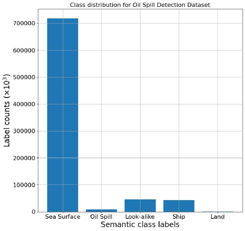
Figure 1: Plot showing the distribution of the semantic classes in the Oil spill detection dataset.

3.2 Image preprocessing and data augmentation

In their research, Marios Krestenitis et al. used smaller image patches to train various models (Krestenitis et al., 2019). The smallest and largest image patch sizes used in their research were $320\times 320$ and $336\times 336$, respectively. In this research, the original images, in $1250\times 650$ dimensions, were padded with patches on all the $4$ sides of the image to produce resulting images of $1280\times 672$. An original sample image from the training set and its corresponding padded image are shown in Figure 2(a) and Figure 2(b), respectively. So, higher resolution images were used as input to the models in this research, compared to those used by Marios Krestenitis et al. (Krestenitis et al., 2019). The patch padding was done in such a way as to select a patch of pixels with the sea surface. To make this patching task easier, a random sample image from the training set was selected. To increase the size of the dataset of the training data, data augmentation was applied. Random horizontal and vertical flips were applied only on the training set for data augmentation. The images were normalized using the mean and standard deviation of the training set. The normalized images were used as input to the various models used in this research.

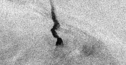
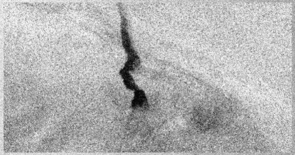
Figure 2: (a) An original sample image from the training set. (b) A sample padded image from the training set.

3.3 Models

3.3.1 Residual networks

Once the CNNs became popular and produced state-of-the-art results, researchers tried deeper CNNs by adding more convolution layers to achieve better accuracy and solve even more complex problems. However, it turned out that making a network deeper after a certain point degraded the model’s accuracy because of the vanishing/exploding gradient problem. To solve the issue mentioned above, Residual Network (ResNet) (He et al., 2015) was introduced by Kaiming He et al. The ResNet consists of residual blocks which can learn identity mappings in case of deeper networks where gradients can vanish. When stacked, these residual blocks help mitigate the vanishing gradient problem by learning an identity function.

In mathematical terms, Let us consider input $x$, and the desired mapping from input to output is denoted by $H(x)$. The residual denoted by $F(x)$ between the output $H(x)$ and input $x$ can be computed using the equation (1)

$$F(x)=H(x)-x$$ (1)

So, instead of using the original mapping, it can be recast into residual mapping using the equation (2)

$$H(x)=F(x)+x$$ (2)

A constraint to performing the above mapping is that $F(x)$ and $x$ should be of the same dimensions. But if that is not the case, then one can use a projection vector $W_{s}$ to match the dimensions. This is shown in equation (3).

$$y=F(x,\{W_{i}\})+W_{s}x$$ (3)

Kaiming He et al. (He et al., 2015) showed that it was easier to learn the residual mapping than the original mapping.

This research used various pre-trained variants of ResNet models — ResNet-18, ResNet-34, ResNet-50, and ResNet-101 encoders, i.e., without the final classification layer used for object recognition on the ImageNet dataset (Deng et al., 2009; Russakovsky et al., 2015; He et al., 2015).

3.3.2 EfficientNet

Neural Architecture Search (NAS) was proposed to optimize network architecture for image classification by Zoph et al. (Zoph et al., 2017). The training bottlenecks of EfficientNet were addressed, and EfficientNetV2 was proposed by Mingxing Tan et al. (Tan et al., 2019; Tan and Le, 2021). The main change was replacing the MBConv block of EfficientNet with a new block proposed by Mingxing Tan et al., the FusedMBConv block, in the early layers. In the MBConv block, a $3\times 3$ depthwise convolution layer was followed by a $1\times 1$ standard convolution layer. This was replaced in the FusedMBConv block with a single fused $3\times 3$ convolution layer. The other changes in EfficientNetV2 were to use $3\times 3$ kernel sizes instead of larger kernel sizes but with more layers and a smaller expansion ratio for MBConv blocks since smaller expansion ratios and removal of the last stride-1 stage, which were optimizations towards a reduction of the memory access overhead (Tan and Le, 2021).

3.3.3 DeepLabV3 and DeepLabV3+

The output of the encoder was provided as the input to the decoder, i.e., one of the decoders considered in this research — DeepLabV3 and DeepLabV3+.

In the DeepLabV3 decoder, Atrous Spatial Pyramid Pooling (ASPP) block was used (Chen et al., 2017, 2016). This was a modification of earlier versions of the DeepLab decoder where atrous convolution layers were used instead of standard convolution layers. A dilation rate is used in atrous or dilated convolution, which uses a larger view of pixels when the kernel is applied to the image. In this ASPP block, there were four atrous convolution layers. In addition, ASPP has an average pooling layer that was used on the feature maps from the encoder block to provide global context information. Finally, the outputs of all these five layers of the ASPP block were concatenated, and bilinear upsampling was applied to produce feature maps with the same dimensions as that of the input image dimensions.

There were some minor changes to the DeepLabV3+ decoder compared to that of DeepLabV2 (Chen et al., 2017, 2018). First, the outputs of all five layers of the ASPP block were concatenated, and bilinear upsampling by a factor of 4 was applied. Then, to the corresponding features from the encoder block, a $1\times 1$ convolution was applied to balance the importance between the backbone’s low-level features and the encoder block’s compressed semantic features. The resulting features were concatenated with upsampled features followed by $3$ convolution layers to refine the concatenated features. This connection from the encoder block and concatenation was a minor change in the DeepLabV3+ decoder. The resulting feature maps were upsampled using bilinear upsampling to produce feature maps with the same dimensions as that of the input image dimensions.

3.4 Training

For training the models, different encoders and decoders were used to perform a comparative study on the overall performance of the models on relatively higher dimensional images. The following encoders were used in this research — ResNet-18, ResNet-34, ResNet-50, ResNet-101, EfficientNetV2S, and EfficientNetV2M (He et al., 2015; Tan and Le, 2021). The pre-trained models trained on the ImageNet dataset were used for the encoder models using transfer learning (Bengio, 2012; Deng et al., 2009; Russakovsky et al., 2015). The following decoders were used in this research — DeepLabV3 and DeepLabV3+ (Chen et al., 2017, 2018). All the encoder-decoder models were trained end to end for 100 epochs.

For training the models, mean categorical cross-entropy loss was used since the dataset contained $5$, semantic classes. The categorical cross-entropy is given by Equation 4 where $c_{i}$ denotes the encoded class and $p_{i}$ denotes the probability of the class as predicted by the model for every one of the $n$ classes in the dataset. The Stochastic Gradient Descent (SGD) optimizer was used with an initial learning rate of $1\times 10^{-2}$, a momentum of $0.9$, and a weight decay of $1\times 10^{-4}$. Liang-Chieh Chen et al. observed that the performance of the segmentation model was higher when SGD was combined with the Polynomial learning rate scheduler (Chen et al., 2016). In this research, the SGD optimizer was combined with a Polynomial learning rate scheduler, where the learning rate is decayed in a polynomial fashion. The Polynomial learning rate scheduler is given by Equation 5 where $lr_{0}$ is the initial learning rate, $e$ is the current epoch, $T_{e}$ is the total number of epochs, and $power$ controls the learning rate decay. Once the learning rate at any epoch goes below a certain threshold and becomes closer to zero, learning may be hampered. To avoid this, a minimum learning rate was used as a threshold, and if the learning rate went below the threshold, the threshold learning rate would be used. For the Polynomial learning rate scheduler, the parameters — $lr_{0}$ was set to $1\times 10^{-2}$, $power$ was set to $0.9$ and the minimum learning rate was set to $1\times 10^{-6}$.

$$CE(c,p)=\sum_{i=1}^{n}c_{i}\log(p_{i})$$ (4)

$$lr=lr_{0}\times(1-\frac{e}{T_{e}})^{power}$$ (5)

A weight decay was used for regularization in the SGD optimizer, a dropout layer with a dropout rate of $10\%$, and data augmentation with horizontal and vertical flips was used.

Different batch sizes were used to train different models as they differ in the number of parameters that require different amounts of Graphical Processing Unit (GPU) memory. Table 1 shows the batch size that was used to train different models. The models were trained by the Nvidia V100 GPU available on the Peregrine high-performance computing cluster.

Table 1: Batch size of different models used for training.

Encoder	Decoder	#Params	Batch
		(millions)	size
ResNet-18	DeepLabV3+	12.34	32
ResNet-34	DeepLabV3+	22.45	24
ResNet-50	DeepLabV3+	25.07	8
ResNet-101	DeepLabV3+	44.06	8
EfficientNetV2S	DeepLabV3	21.42	8
EfficientNetV2M	DeepLabV3	54.11	4

3.5 Transfer learning

Transfer learning is a machine learning paradigm where the process of training very deep neural networks becomes less tedious (Bengio, 2012). By using transfer learning, one can apply a previously learned machine learning model on some task to a different task, but which are related. This technique has become very popular in the field of computer vision due to the impressive ability of CNNs to apply the learned low-level feature extraction on different tasks. The other reason is that training these models from scratch is both computationally and economically expensive. Transfer learning has enabled researchers to get a reasonable accuracy while reducing the training time compared to retraining the models from scratch for every task.

3.6 Evaluation metrics

For evaluation of the performance of the models, Intersection over Union (IoU) was used (Krestenitis et al., 2019). The mean IoU (m-IoU) is the mean of the IoU of the different semantic classes in the dataset. The class IoU is the IoU computed for a semantic class individually.

4 Results and Discussion

4.1 Quantitative results

A 5-fold cross-validation was performed to find the deviation of the performance of the models on different random validation splits. Table 2 shows the performance metrics of the various models for a 5-fold validation on the randomized validation sets. For all the models, there is a significant deviation of m-IoU (greater than $1\%$) across a 5-fold validation. This is as expected since the dataset is highly imbalanced and was split randomly into training and validation sets. Furthermore, some splits would have higher m-IoU than others, depending on the division of the samples and their distribution of semantic classes. So, the m-IoU of the validation set clearly depends on the split in cross-validation experiments.

Table 2: Performances of various models for five-fold cross-validation.

Encoder	Decoder	m-IoU ($\%$)
ResNet-18	DeepLabV3+	$67.345\pm 1.407$
ResNet-34	DeepLabV3+	$67.522\pm 3.898$
ResNet-50	DeepLabV3+	$67.578\pm 3.631$
ResNet-101	DeepLabV3+	$68.152\pm 2.470$
EfficientNetV2S	DeepLabV3	$60.668\pm 2.796$
EfficientNetV2M	DeepLabV3	$58.997\pm 3.021$

Table 3 shows the performance metrics of the best-performing model for each of the models on the test set with $102$ images. The best m-IoU on the test set was $64.868\%$ for the model with the ResNet-50 encoder and DeepLabV3+ decoder. This model’s performance is slightly lower than the best-performing model from the research by Mario Krestenitis et al., which scored m-IoU of $65.06\%$ on the test set (Krestenitis et al., 2019). Table 1 also shows the number of parameters in various models. If the model with EfficientNetV2M encoder and DeepLabV3 decoder with 54.11 million parameters and the model with ResNet-50 encoder and DeepLabV3+ decoder with just 25.07 million parameters are considered, their performances are $55.504\%$ and $64.868\%$ respectively. So, this shows that increasing the number of parameters in a model would not necessarily improve the model’s performance for every task.

Table 3: Model performance on the unseen test set of $102$ images.

Encoder	Decoder	m-IoU ($\%$)
ResNet-18	DeepLabV3+	59.647
ResNet-34	DeepLabV3+	60.843
ResNet-50	DeepLabV3+	64.868
ResNet-101	DeepLabV3+	64.677
EfficientNetV2S	DeepLabV3	55.492
EfficientNetV2M	DeepLabV3	55.504

Table 4 shows the class-wise performance metrics of the best-performing models on the test set with $102$ images, i.e., the model with ResNet-50 encoder and DeepLabV3+ decoder from this research and best-performing model from Marios Krestenitis et al. research. Marios et al. best model scored a class IoU of $53.38\%$ and $55.40\%$ for the "oil spill" and "oil spill look-alike" classes, respectively (Krestenitis et al., 2019). On the other hand, the best-performing model from this research scored a class IoU of $61.549\%$ and $40.773\%$ for the "oil spill" and "oil spill look-alike" classes, respectively. Although the model from this research scored lower for the "oil spill look-alike" class, it still scored higher for the "oil spill" class, which is of more interest. Another observation is that the performance of detection of "ship" is more remarkable for the best-performing model from this research when compared with that of the best-performing model from Marios Krestenitis et al., with class IoU of $33.378\%$ and $27.63\%$ respectively. For the remaining classes, i.e., the "sea surface" and "land", the performances of the best-performing models from this research and Marios Krestenitis et al. are comparable.

Table 4: Class-wise performance, i.e., the class IoU of the best-performing model on the test set of $102$ images.

	Class IoU ($\%$)
	Our best	Best model of
	model	Marios et al.
Semantic Class
Sea surface	96.422	96.43
Oil spill	61.549	53.38
Oil spill look-alike	40.773	55.40
Ship	33.378	27.63
Land	92.218	92.44
mean	64.868	65.06

4.2 Qualitative results

A few test set samples, their ground-truth masks, and their predictions with the best-performing model from this research are presented. From the test sample shown in Figure 3(a), its ground-truth mask shown in Figure 3(b) and its prediction mask shown in Figure 3(c), it can be observed that relatively smaller areas of "oil spills" (in Cyan) along with "ships" (in Brown) are detected by the model with reasonable accuracy, for this sample. From Figure 4(a), Figure 4(b), and Figure 4(c), it can be observed that relatively more significant areas of "oil spills" are detected by the model with reasonable accuracy. In this test sample, the model gets confused with the "oil spill" and "oil spill look-alike" classes, and portions of the regions are predicted as belonging to these two classes; however, from Figure 5(a), Figure 5(b), and Figure 5(c), it can be observed that relatively more significant areas of "oil spills" are not detected by the model with reasonable accuracy. So, there are both good and not-so-good detections by the model. From Figure 6(a), Figure 6(b), and Figure 6(c), it can be observed that relatively smaller areas of "oil spill" are detected by the model with reasonable accuracy. From Figure 7(a), Figure 7(b), and Figure 7(c), it can be observed that relatively smaller areas of "oil spill" are not detected by the model with good accuracy.

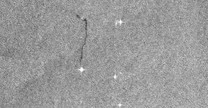
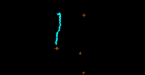
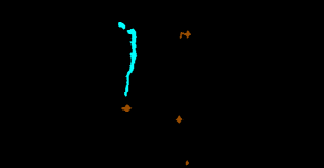
Figure 3: (a) Sample test image (b) Groundtruth (c) Predicted mask.

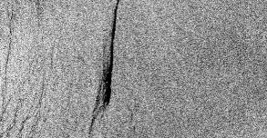
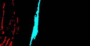
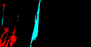
Figure 4: (a) Sample test image (b) Groundtruth (c) Predicted mask.

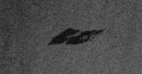
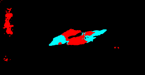
Figure 5: (a) Sample test image (b) Groundtruth (c) Predicted mask.

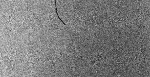
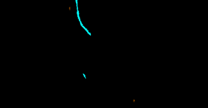
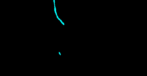
Figure 6: (a) Sample test image (b) Groundtruth (c) Predicted mask.

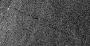
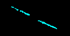
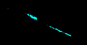
Figure 7: (a) Sample test image (b) Groundtruth (c) Predicted mask.

4.3 Learning curves

Figure 8(a) shows the plot of losses for training and validation sets vs. epoch for the model with ResNet-50 encoder and DeepLabV3+ decoder, i.e., for the best-performing models from our experiments. Figure 8(b) shows the plot of m-IoU for validation set vs. epoch for the model with ResNet-50 encoder and DeepLabV3+ decoder.

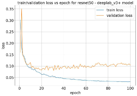
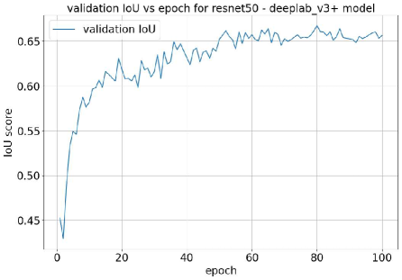
Figure 8: (a) Plot of training and validation losses for the model with ResNet-50 encoder and DeepLabV3+ decoder; (b) Plot of validation m-IoU for the model with ResNet-50 encoder and DeepLabV3+ decoder.

5 Conclusions

In the research by Marios Krestenitis et al., the high-dimensional images were divided into smaller patches that were used as input for their models. The best-performing model scored an m-IoU of $65.06\%$ and a class IoU of $53.38\%$. This research used high-dimensional images as input to the model without dividing them into multiple patches. The best-performing model from this research, with ResNet-50 encoder and DeepLabV3+ decoder, scored an m-IoU of $64.868\%$ and a class IoU of $61.549\%$ for the "oil spill" class. So, using high dimensional images has its benefits and results in higher performance of "oil spill" detection. Since there are also image samples in the dataset with the "oil spill look-alike" class, the trained models sometimes get confused with the "oil spill" and "oil spill look-alike" classes which is still a challenge. There are various other encoders and decoders that can be experimented with. Also, there is room for improvement with the current encoders and decoders used in this research by incorporating visual self-attention modules. However, these can be explored in the future.

References

- Dunnet et al. (1982) G. M. Dunnet, Dennis John Crisp, G. Conan, R. Bournaud, H. A. Cole, and R.B. Clark. Oil pollution and seabird populations. Philosophical Transactions of the Royal Society of London. B, Biological Sciences, 297(1087):413–427, 1982. doi:10.1098/rstb.1982.0051. URL https://royalsocietypublishing.org/doi/abs/10.1098/rstb.1982.0051.
- Middlebrook et al. (2010) Ann Middlebrook, Ravan Ahmadov, Elliot Atlas, Roya Bahreini, D. Blake, J. Brioude, C. Brock, Joost de Gouw, D. Fahey, Fred Fehsenfeld, John Holloway, Richard Lueb, Stuart McKeen, J. Meagher, Simone Meinardi, D. Murphy, David Parrish, Jeff Peischl, and Laurence Watts. Air quality impact of the deepwater horizon oil spill (invited). AGU Fall Meeting Abstracts, pages 02–, 12 2010.
- BROEKEMA (2016) WOUT BROEKEMA. Crisis-induced learning and issue politicization in the eu: The braer, sea empress, erika, and prestige oil spill disasters. Public Administration, 94(2):381–398, 2016. doi:https://doi.org/10.1111/padm.12170. URL https://onlinelibrary.wiley.com/doi/abs/10.1111/padm.12170.
- lon (2010) Hindsight and foresight: 20 years after the exxon valdez spill. NOAA Ocean Media Center, 2010.
- Deng et al. (2009) J. Deng, W. Dong, R. Socher, L.-J. Li, K. Li, and L. Fei-Fei. ImageNet: A Large-Scale Hierarchical Image Database. In CVPR09, 2009.
- Russakovsky et al. (2015) Olga Russakovsky, Jia Deng, Hao Su, Jonathan Krause, Sanjeev Satheesh, Sean Ma, Zhiheng Huang, Andrej Karpathy, Aditya Khosla, Michael Bernstein, Alexander C. Berg, and Li Fei-Fei. ImageNet Large Scale Visual Recognition Challenge. International Journal of Computer Vision (IJCV), 115(3):211–252, 2015. doi:10.1007/s11263-015-0816-y.
- Krizhevsky et al. (2012) Alex Krizhevsky, Ilya Sutskever, and Geoffrey E Hinton. Imagenet classification with deep convolutional neural networks. In F. Pereira, C.J. Burges, L. Bottou, and K.Q. Weinberger, editors, Advances in Neural Information Processing Systems, volume 25. Curran Associates, Inc., 2012. URL https://proceedings.neurips.cc/paper/2012/file/c399862d3b9d6b76c8436e924a68c45b-Paper.pdf.
- Krestenitis et al. (2019) Marios Krestenitis, Georgios A. Orfanidis, Konstantinos Ioannidis, Konstantinos Avgerinakis, Stefanos Vrochidis, and Yiannis Kompatsiaris. Oil spill identification from satellite images using deep neural networks. Remote. Sens., 11:1762, 2019.
- LeCun et al. (1989) Y. LeCun, B. Boser, J. S. Denker, D. Henderson, R. E. Howard, W. Hubbard, and L. D. Jackel. Backpropagation applied to handwritten zip code recognition. Neural Computation, 1(4):541–551, 1989. doi:10.1162/neco.1989.1.4.541.
- LeCun et al. (1998) Y. LeCun, L. Bottou, Y. Bengio, and P. Haffner. Gradient-based learning applied to document recognition. Proceedings of the IEEE, 86(11):2278–2324, 1998. doi:10.1109/5.726791.
- (11) Y. LeCun. The mnist database of handwritten digits. http://yann.lecun.com/exdb/mnist/. URL https://cir.nii.ac.jp/crid/1571417126193283840.
- Long et al. (2014) Jonathan Long, Evan Shelhamer, and Trevor Darrell. Fully convolutional networks for semantic segmentation. CoRR, abs/1411.4038, 2014. URL http://arxiv.org/abs/1411.4038.
- Ronneberger et al. (2015) Olaf Ronneberger, Philipp Fischer, and Thomas Brox. U-net: Convolutional networks for biomedical image segmentation. CoRR, abs/1505.04597, 2015. URL http://arxiv.org/abs/1505.04597.
- Chaurasia and Culurciello (2017) Abhishek Chaurasia and Eugenio Culurciello. Linknet: Exploiting encoder representations for efficient semantic segmentation. CoRR, abs/1707.03718, 2017. URL http://arxiv.org/abs/1707.03718.
- Zhao et al. (2016) Hengshuang Zhao, Jianping Shi, Xiaojuan Qi, Xiaogang Wang, and Jiaya Jia. Pyramid scene parsing network. CoRR, abs/1612.01105, 2016. URL http://arxiv.org/abs/1612.01105.
- Chen et al. (2018) Liang-Chieh Chen, Yukun Zhu, George Papandreou, Florian Schroff, and Hartwig Adam. Encoder-decoder with atrous separable convolution for semantic image segmentation. CoRR, abs/1802.02611, 2018. URL http://arxiv.org/abs/1802.02611.
- Lin et al. (2014) Tsung-Yi Lin, Michael Maire, Serge J. Belongie, Lubomir D. Bourdev, Ross B. Girshick, James Hays, Pietro Perona, Deva Ramanan, Piotr Dollár, and C. Lawrence Zitnick. Microsoft COCO: common objects in context. CoRR, abs/1405.0312, 2014. URL http://arxiv.org/abs/1405.0312.
- Cordts et al. (2016) Marius Cordts, Mohamed Omran, Sebastian Ramos, Timo Rehfeld, Markus Enzweiler, Rodrigo Benenson, Uwe Franke, Stefan Roth, and Bernt Schiele. The cityscapes dataset for semantic urban scene understanding. In Proc. of the IEEE Conference on Computer Vision and Pattern Recognition (CVPR), 2016.
- He et al. (2015) Kaiming He, Xiangyu Zhang, Shaoqing Ren, and Jian Sun. Deep residual learning for image recognition. CoRR, abs/1512.03385, 2015. URL http://arxiv.org/abs/1512.03385.
- Sandler et al. (2018) Mark Sandler, Andrew G. Howard, Menglong Zhu, Andrey Zhmoginov, and Liang-Chieh Chen. Inverted residuals and linear bottlenecks: Mobile networks for classification, detection and segmentation. CoRR, abs/1801.04381, 2018. URL http://arxiv.org/abs/1801.04381.
- Zoph et al. (2017) Barret Zoph, Vijay Vasudevan, Jonathon Shlens, and Quoc V. Le. Learning transferable architectures for scalable image recognition. CoRR, abs/1707.07012, 2017. URL http://arxiv.org/abs/1707.07012.
- Tan et al. (2019) Mingxing Tan, Ruoming Pang, and Quoc V. Le. Efficientdet: Scalable and efficient object detection. CoRR, abs/1911.09070, 2019. URL http://arxiv.org/abs/1911.09070.
- Tan and Le (2021) Mingxing Tan and Quoc V. Le. Efficientnetv2: Smaller models and faster training. CoRR, abs/2104.00298, 2021. URL https://arxiv.org/abs/2104.00298.
- Chen et al. (2017) Liang-Chieh Chen, George Papandreou, Florian Schroff, and Hartwig Adam. Rethinking atrous convolution for semantic image segmentation. CoRR, abs/1706.05587, 2017. URL http://arxiv.org/abs/1706.05587.
- Chen et al. (2016) Liang-Chieh Chen, George Papandreou, Iasonas Kokkinos, Kevin Murphy, and Alan L. Yuille. Deeplab: Semantic image segmentation with deep convolutional nets, atrous convolution, and fully connected crfs. CoRR, abs/1606.00915, 2016. URL http://arxiv.org/abs/1606.00915.
- Bengio (2012) Yoshua Bengio. Deep learning of representations for unsupervised and transfer learning. In Isabelle Guyon, Gideon Dror, Vincent Lemaire, Graham Taylor, and Daniel Silver, editors, Proceedings of ICML Workshop on Unsupervised and Transfer Learning, volume 27 of Proceedings of Machine Learning Research, pages 17–36, Bellevue, Washington, USA, 02 Jul 2012. PMLR. URL https://proceedings.mlr.press/v27/bengio12a.html.